Study of Robust Diffusion Recursive Least Squares Algorithms with Side Information for Networked Agents

Abstract

This work develops a robust diffusion recursive least squares algorithm to mitigate the performance degradation often experienced in networks of agents in the presence of impulsive noise. This algorithm minimizes an exponentially weighted least-squares cost function subject to a time-dependent constraint on the squared norm of the intermediate estimate update at each node. With the help of side information, the constraint is recursively updated in a diffusion strategy. Moreover, a control strategy for resetting the constraint is also proposed to retain good tracking capability when the estimated parameters suddenly change. Simulations show the superiority of the proposed algorithm over previously reported techniques in various impulsive noise scenarios.

Index Terms—  Diffusion cooperation, distributed algorithms, impulsive noises, robust recursive least squares.

1 Introduction

In the last decade, distributed adaptive algorithms for estimating parameters of interest over wireless sensor networks with multiple nodes (or agents) have attracted significant attention, due to their performance advantages and robustness [1]. The core idea is that each node performs adaptive estimation, in cooperation with its neighboring nodes. Distributed adaptive algorithms have been applied to many problems, e.g., frequency estimation in power grid [2] and spectrum estimation [3]. According to the cooperation strategy of interconnected nodes, existing algorithms can be categorized as the incremental [4], consensus [5], and diffusion [6, 7, 8] types. The diffusion type is the most popular [5], because it does not require a Hamiltonian cycle path as does the incremental type [4]; it is stable and has a better estimation performance than the consensus type [5]. Several diffusion-based distributed algorithms have been proposed such as the diffusion least mean square (dLMS) algorithm [6], diffusion conjugate gradient (dCG) [9], diffusion recursive least squares (dRLS) algorithm [7], and their modifications [10, 11, 12, 13, 14].

In practice, measurements at the network nodes can be corrupted by impulsive noise [15]. An impulsive noise process has the property that its occurence probability is small and the magnitude is typically much larger than the nominal measurement. It is well-known that the impulsive noise deteriorates significantly the performance of algorithms in the single-agent case. For distributed algorithms in the multi-agent case, impulsive noise can propagate over the entire network due to the exchange of information among nodes. To reduce the impulsive noise interference, many robust distributed algorithms have been proposed [16, 17, 18, 19, 20, 21, 22, 23, 24]. Some algorithms, e.g., the diffusion sign error LMS (dSE-LMS) [16], are based on using the instantaneous gradient-descent method to minimize an individual robust criterion. In [17], a robust variable weighting coefficients dLMS (RVWC-dLMS) algorithm was developed, which only considers the data and intermediate estimates from nodes not affected by impulsive noise; this is based on a judgement whether impulsive noise samples occur or not. However, these robust algorithms have slow convergence, especially for colored input signals.

RLS-based algorithms have a good decorrelating property for colored signals, thereby providing fast convergence. In this paper, therefore, we present a robust dRLS (R-dRLS) algorithm for distributed estimation over networks affected by impulsive noise. The R-dRLS algorithm minimizes a local exponentially weighted least-squares (LS) cost function subject to a time-dependent constraint on the squared norm of the intermediate estimate at each node. Unlike the framework in [25], we consider here a multi-agent scenario with the diffusion strategy. Furthermore, in order to equip the R-dRLS algorithm with the ability to withstand sudden changes in the environment, we also propose a diffusion-based distributed nonstationary control (DNC) method. This paper is organized as follows. In Section 2, the estimation problem in the network is described. In Section 3, the proposed algorithm is derived. In Section 4, results of simulation in impulsive noise scenarios are presented. Finally, conclusions are given in Section 5.

2 Problem Formulation

Let us consider a network that has $N$ nodes distributed over some region in space, where a link between two nodes means that they can communicate directly with each other. The neighborhood of node k is denoted by $\mathcal{N}_{k}$, i.e., a set of all nodes connected to node $k$ including itself. The cardinality of $\mathcal{N}_{k}$ is denoted by $n_{k}$. At every time instant $i\geq 0$, every node k observes a data regressor vector $\bm{u}_{k,i}$ of size $M\times 1$ and a scalar measurement $d_{k}(i)$, related as:

$$d_{k}(i)=\bm{u}_{k,i}^{T}\bm{w}^{o}+v_{k}(i),$$ (1)

where the superscript $T$ denotes the transpose, $\bm{w}^{o}$ is a parameter vector of size $M\times 1$, and $v_{k}(i)$ is the additive noise at node k. The regressors $\bm{u}_{k,i}$ and $\bm{u}_{l,j}$ are spatially independent for $k\neq l$ and all $i,j$. The additive noises $v_{k}(i)$ and $v_{l}(j)$ are spatially and temporally independent for $k\neq l$ and $i\neq j$. Moreover, any $\bm{u}_{k,i}$ is independent of any $v_{l}(j)$. The model (1) is widely used in many applications [1, 26].

The task is to estimate $\bm{w}^{o}$, using the available data collected at nodes, i.e., $\{\bm{u}_{k,i},d_{k}(i)\}_{k=1}^{N}$. For this purpose, the global LS-based estimation problem is described as [7]:

$$\begin{array}[]{rcl}\begin{aligned} &\bm{w}_{i}=\arg\min\limits_{\bm{w}}\\ &\left\{\lambda^{i+1}\delta\lVert\bm{w}\rVert_{2}^{2}+\sum\limits_{j=0}^{i}\lambda^{i-j}\sum\limits_{k=1}^{N}\left(d_{k}(j)-\bm{u}_{k,i}^{T}\bm{w}\right)^{2}\right\},\end{aligned}\end{array}$$ (2)

where $\lVert\cdot\rVert_{2}$ denotes the $l_{2}$-norm of a vector, $\delta>0$ is a regularization constant, and $\lambda$ is the forgetting factor. The dRLS algorithm solves (2) in a distributed manner [7]. In practice, $v_{k}(i)$ may contain impulsive noise, severely corrupting the measurement $d_{k}(i)$. With such noise processes, the algorithms obtained from (2), e.g., the dRLS algorithm, would fail to work.

3 Proposed Distributed Algorithm

3.1 Derivation of the R-dRLS Algorithm

We focus here on the adapt-then-combine (ATC) implementation of the diffusion strategy, which has been shown to outperform the combine-then-adapt (CTA) implementation [5]. Following the ATC-based diffusion strategy [6, 7], i.e., performing first the adaptation step and then the combination step, the R-dRLS algorithm will be derived in the sequel. We start with the adaptation step. Every node $k$, at time instant $i$, finds an intermediate estimate $\bm{\psi}_{k,i}$ of $\bm{w}^{o}$ by minimizing the individual local cost function:

$$\begin{array}[]{rcl}\begin{aligned} J_{k}(\bm{\psi}_{k,i})=&\lVert\bm{\psi}_{k,i}-\bm{w}_{k,i-1}\rVert_{\bm{Q}_{k,i}}^{2}\\ &+[d_{k}(i)-\bm{u}_{k,i}^{T}\bm{\psi}_{k,i}]^{2},\end{aligned}\end{array}$$ (3)

with $\bm{Q}_{k,i}=\bm{R}_{k,i}-\bm{u}_{k,i}\bm{u}_{k,i}^{T}$, where

$$\begin{array}[]{rcl}\begin{aligned} \bm{R}_{k,i}\triangleq&\lambda^{i+1}\delta\bm{I}+\sum\limits_{j=0}^{i}\lambda^{i-j}\bm{u}_{k,j}\bm{u}_{k,j}^{T}\\ =&\lambda\bm{R}_{k,i-1}+\bm{u}_{k,i}\bm{u}_{k,i}^{T}\end{aligned}\end{array}$$ (4)

is the time-averaged correlation matrix for the regression vector at node $k$ and $\bm{w}_{k,i-1}$ is an estimate of $\bm{w}^{o}$ at node $k$ at time instant $i-1$. Notice that the form $\lVert\bm{x}\rVert_{\bm{Q}}^{2}\triangleq\bm{x}^{T}\bm{Q}\bm{x}$ in (3) defines the Riemmanian distance [27] between vectors $\bm{\psi}_{k,i}$ and $\bm{w}_{k,i-1}$. Setting the derivative of $J_{k}(\bm{\psi}_{k,i})$ with respect to $\bm{\psi}_{k,i}$ to zero, we obtain

$$\begin{array}[]{rcl}\begin{aligned} \bm{\psi}_{k,i}=\bm{w}_{k,i-1}+\bm{P}_{k,i}\bm{u}_{k,i}e_{k}(i),\\ \end{aligned}\end{array}$$ (5)

where $e_{k}(i)=d_{k}(i)-\bm{u}_{k,i}^{T}\bm{w}_{k,i-1}$ stands for the output error at node $k$ and $\bm{P}_{k,i}\triangleq\bm{R}_{k,i}^{-1}$. Using the matrix inversion lemma [26], we have

$$\begin{array}[]{rcl}\begin{aligned} \bm{P}_{k,i}=\frac{1}{\lambda}\left(\bm{P}_{k,i-1}-\frac{\bm{P}_{k,i-1}\bm{u}_{k,i}\bm{u}_{k,i}^{T}\bm{P}_{k,i-1}}{\lambda+\bm{u}_{k,i}^{T}\bm{P}_{k,i-1}\bm{u}_{k,i}}\right),\\ \end{aligned}\end{array}$$ (6)

where $\bm{P}_{k,i}$ is initialized as $\left.\bm{P}_{k,0}=\delta^{-1}\bm{I}\right.$ and $\bm{I}$ is an identity matrix. Since $\bm{w}_{k,i-1}=\bm{R}_{k,i-1}^{-1}\bm{z}_{k,i-1}$, where $\bm{z}_{k,i}=\lambda\bm{z}_{k,i-1}+\bm{u}_{k,i}d_{k}(i)$, (5) means that every node $k$ performs an RLS update. However, with the update (5), the adverse effect of an impulsive noise sample at time instant $i$ will propagate through nodes via $e_{k}(i)$. This effect can last for many iterations. To make the algorithm robust in impulsive noise scenarios, we propose to minimize (3) under the following constraint:

$$\begin{array}[]{rcl}\begin{aligned} \lVert\bm{\psi}_{k,i}-\bm{w}_{k,i-1}\rVert_{2}^{2}\leq\xi_{k}(i-1),\end{aligned}\end{array}$$ (7)

where $\xi_{k}(i)$ is a positive bound. This constraint is employed to enforce the squared norm of the update of the intermediate estimate not to exceed the amount $\xi_{k}(i-1)$ regardless of the type of noise (possibly, impulsive noise), thereby guaranteeing the robustness of the algorithm. If (5) satisfies (7), i.e.,

$$\begin{array}[]{rcl}\begin{aligned} \lVert\bm{g}_{k,i}\rVert_{2}\lvert e_{k}(i)\rvert\leq\sqrt{\xi_{k}(i-1)},\end{aligned}\end{array}$$ (8)

where $\left.\bm{g}_{k,i}\triangleq\bm{P}_{k,i}\bm{u}_{k,i}\right.$ represents the Kalman gain vector, then (5) is a solution of the above constrained minimization problem. On the other hand, if (8) is not satisfied (usually in the case of appearance of impulsive noise samples), i.e., $\left.\lVert\bm{g}_{k,i}\rVert_{2}\lvert e_{k}(i)\rvert>\sqrt{\xi_{k}(i-1)}\right.$, we propose to replace the update (5) by a normalized form to satisfy the constraint (7), which is described by

$$\begin{array}[]{rcl}\begin{aligned} \bm{\psi}_{k,i}=\bm{w}_{k,i-1}+\sqrt{\xi_{k}(i-1)}\frac{\bm{g}_{k,i}}{\lVert\bm{g}_{k,i}\rVert_{2}}\text{sign}(e_{k}(i)),\\ \end{aligned}\end{array}$$ (9)

where $\text{sign}(\cdot)$ is the sign function. Consequently, combining (5), (8) and (9), we obtain the adaptation step for each node $k$ as:

$$\begin{array}[]{rcl}\begin{aligned} \bm{\psi}_{k,i}=\bm{w}_{k,i-1}+\min\left[\frac{\sqrt{\xi_{k}(i-1)}}{\lVert\bm{g}_{k,i}\rVert_{2}\lvert e_{k}(i)\rvert},\;1\right]\bm{g}_{k,i}e_{k}(i).\\ \end{aligned}\end{array}$$ (10)

Then, at the combination step, the intermediate estimates $\psi_{m,i}$ from the neigborhood $m\in\mathcal{N}_{k}$ of node $k$ are linearly weighed, yielding a more reliable estimate $\bm{w}_{k,i}$ [1]:

$$\begin{array}[]{rcl}\begin{aligned} \bm{w}_{k,i}=\sum\limits_{m\in\mathcal{N}_{k}}c_{m,k}\bm{\psi}_{m,i},\end{aligned}\end{array}$$ (11)

where the combination coefficients $\{c_{m,k}\}$ are non-negative, and satisfy:

$$\sum\limits_{m\in\mathcal{N}_{k}}c_{m,k}=1\text{, and }c_{m,k}=0\text{ if }m\notin\mathcal{N}_{k}.$$ (12)

Note that, $c_{m,k}$ is a weight that node $k$ assigns to the intermediate estimate $\bm{\psi}_{m,i}$ received from its neighbor node $m$. In general, $\{c_{m,k}\}$ are determined by a static rule (e.g., the Metropolis rule [28] that we adopt in this paper) which keeps them constant in the estimation, or an adaptive rule [28]. It is evident that the bound $\xi_{k}(i)$ controls the robustness of the algorithm against impulsive noise and influences its dynamic behavior, so choosing its value properly is of fundamental importance. To this end, motivated by the single-agent case in [25], $\xi_{k}(i)$ is adjusted recursively based on the diffusion strategy as:

$$\begin{array}[]{rcl}\begin{aligned} \zeta_{k}(i)=&\beta\xi_{k}(i-1)+(1-\beta)\left\|\bm{\psi}_{k,i}-\bm{w}_{k,i-1}\right\|_{2}^{2}\\ =\beta\xi_{k}&(i-1)+(1-\beta)\min[\lVert\bm{g}_{k,i}\rVert_{2}^{2}e_{k}^{2}(i),\xi_{k}(i-1)],\\ \xi_{k}(i)=&\sum\limits_{m\in\mathcal{N}_{k}}c_{m,k}\zeta_{m}(i),\end{aligned}\end{array}$$ (13)

where $\beta$ is a forgetting factor, $0<\beta\lesssim 1$. In (13), at every node $k$, $\xi_{k}(i)$ can be initialized as $\xi_{k}(0)=E_{c}\sigma_{d,k}^{2}/(M\sigma_{u,k}^{2})$, where $E_{c}$ is a positive integer, and $\sigma_{d,k}^{2}$ and $\sigma_{u,k}^{2}$ are powers of signals $d_{k}(i)$ and $\bm{u}_{k,i}$, respectively. The proposed algorithm is shown in Table 1.

Table 1: Proposed R-$\rm d$RLS Algorithm with the DNC Method.

Parameters: $0<\beta\lesssim 1$, $\lambda$, $\delta$ and $E_{c}$ (R-dRLS); $\varrho$ and $t_{\text{th}}$ (DNC)

Initialization: $\bm{w}_{k,0}=\bm{0}$, $\bm{P}_{k,0}=\delta^{-1}\bm{I}$ and $\xi_{k}(0)=E_{c}\frac{\sigma_{d,k}^{2}}{M\sigma_{u,k}^{2}}$ (R-dRLS);

$\varTheta_{\text{old},k}=\varTheta_{\text{new},k}=0$, $V_{t}=\varrho M$, and $V_{d}=0.75V_{t}$ (DNC)

R-dRLS algorithm:

$e_{k}(i)=d_{k}(i)-\bm{u}_{k,i}^{T}\bm{w}_{k,i-1}$

$\bm{P}_{k,i}=\frac{1}{\lambda}\left(\bm{P}_{k,i-1}-\frac{\bm{P}_{k,i-1}\bm{u}_{k,i}\bm{u}_{k,i}^{T}\bm{P}_{k,i-1}}{\lambda+\bm{u}_{k,i}^{T}\bm{P}_{k,i-1}\bm{u}_{k,i}}\right)$

$\bm{g}_{k,i}=\bm{P}_{k,i}\bm{u}_{k,i}$

$\bm{\psi}_{k,i}=\bm{w}_{k,i-1}+\min\left[\frac{\sqrt{\xi_{k}(i-1)}}{\lVert\bm{g}_{k,i}\rVert_{2}\lvert e_{k}(i)\rvert},\;1\right]\bm{g}_{k,i}e_{k}(i)$

$\bm{w}_{k,i}=\sum\limits_{m\in\mathcal{N}_{k}}c_{m,k}\bm{\psi}_{m,i}$

DNC method:

Step 1: to compute $\varDelta_{k}(i)$

if $i=nV_{t},n=0,1,2,...$

$\bm{a}_{k,i}^{T}=\mathcal{O}\left(\left[\frac{e_{k}^{2}(i)}{\|\bm{u}_{k,i}\|_{2}^{2}},\frac{e_{k}^{2}(i-1)}{\|\bm{u}_{k,i-1}\|_{2}^{2}},\text{...},\frac{e_{k}^{2}(i-V_{t}+1)}{\|\bm{u}_{k,i-V_{t}+1}\|_{2}^{2}}\right]\right)$

$\varTheta_{\text{new},k}=\sum\limits_{m\in\mathcal{N}_{k}}c_{m,k}\frac{\bm{a}_{m,i}^{T}\bm{e}}{V_{t}-V_{d}}$

$\varDelta_{k}(i)=\frac{\varTheta_{\text{new},k}-\varTheta_{\text{old},k}}{\xi_{k}(i-1)}$

end

Step 2: to reset $\xi_{k}(i)$

if $\varDelta_{k}(i)>t_{\text{th}}$

$\zeta_{k}(i)=\xi_{k}(0)$, $\bm{P}_{k,i}=\bm{P}_{k,0}$

elseif   $\varTheta_{\text{new},k}>\varTheta_{\text{old},k}$

$\zeta_{k}(i)=\xi_{k}(i-1)+(\varTheta_{\text{new},k}-\varTheta_{\text{old},k})$

else

$\zeta_{k}(i)=\beta\xi_{k}(i-1)+(1-\beta)\min\left[\lVert\bm{g}_{k,i}\rVert_{2}^{2}e_{k}^{2}(i),\;\xi_{k}(i-1)\right]$

end

$\xi_{k}(i)=\sum\limits_{m\in\mathcal{N}_{k}}c_{m,k}\zeta_{m}(i)$

$\varTheta_{\text{old},k}=\varTheta_{\text{new},k}$

Remark: As can be seen from (10), the operation mode of the proposed algorithm is twofold. At time instant $i$, if $\lVert\bm{g}_{k,i}\rVert_{2}^{2}e_{k}^{2}(i)\leq\xi_{k}(i-1)$, the RLS update is performed; if not, the RLS update is normalized to have a norm of value $\xi_{k}(i-1)$. At the early iterations, the values of $\xi_{k}(i)$ can be high compared to $\lVert\bm{g}_{k,i}\rVert_{2}^{2}e_{k}^{2}(i)$ so that the algorithm will behave as the dRLS algorithm, providing a fast convergence. Whenever an impulsive noise sample appears, due to its significant magnitude, the algorithm will work as an dRLS update multiplied by a very small ’step size’ scaling factor given by $\sqrt{\xi_{k}(i-1)}/(\lVert\bm{g}_{k,i}\rVert_{2}|e_{k}(i)|)$, thus suppressing the negative influence of impulsive noise on the estimation [29, 30, 31, 32, 33, 34, 35, 36, 37] and reducing the error propagation effect. The algorithm robustness to impulsive noise is further maintained, due to decreasing $\xi_{k}(i)$ over the iterations. This algorithm can be considered as an improved dRLS algorithm with an additional ’step size’ scaling factor which is time-varying and between 1 and $\sqrt{\xi_{k}(i-1)}/(\lVert\bm{g}_{k,i}\rVert_{2}|e_{k}(i)|)$, as can be observed in (10).

3.2 DNC Method

Although the decreasing values of the sequence $\{\xi_{k}(i)\}$ with the iteration $i$ prompt the R-dRLS algorithm more robust against impulsive noises, the algorithm also loses its tracking capability for a sudden change of the unknown vector $\bm{w}^{o}$. To improve the tracking capability, referring to the single-agent scenario [38], we also develop a diffusion-based DNC method, summarized in Table 1. The DNC method includes two implementation procedures.

Firstly, a variable $\varDelta_{k}(i)$ at node $k$ is computed once for every $V_{t}$ iterations, to judge whether the unknown vector has a change or not. In this step, $\bm{a}_{k,i}^{T}=\mathcal{O}\left(\left[\frac{e_{k}^{2}(i)}{\|\bm{u}_{k,i}\|_{2}^{2}},\frac{e_{k}^{2}(i-1)}{\|\bm{u}_{k,i-1}\|_{2}^{2}},\text{...},\frac{e_{k}^{2}(i-V_{t}+1)}{\|\bm{u}_{k,i-V_{t}+1}\|_{2}^{2}}\right]\right)$ with $\mathcal{O}(\cdot)$ denoting the ascending arrangement for its arguments, and $\bm{e}=[1,...,1,0,...,0]^{T}$ is a vector whose first $V_{t}-V_{d}$ elements set to one, where $V_{d}$ is a positive integer with $V_{d}<V_{t}$. Thus, the product $\bm{a}_{k,i}^{T}\bm{e}$ can remove the effect of outliers (e.g., impulsive noise samples) on the rightness of the computation of $\varDelta_{k}(i)$. Typically, for both $V_{t}$ and $V_{d}$, good choices are $V_{t}=\varrho M$ with $\varrho=1\sim 3$ and $V_{d}=0.75V_{t}$ [38]. Note that, for large occurence probability of impulsive noise, the value of $V_{t}-V_{d}$ should be decreased to discard the impulsive noise samples.

Secondly, if $\varDelta_{k}(i)>t_{\text{th}}$, where $t_{\text{th}}$ is a predefined threshold, meaning a change of $\bm{w}^{o}$ has occured, then we need to reset $\xi_{k}(i)$ to its initial value $\xi_{k}(0)$. More importantly, $\bm{P}_{k,i}$ is also re-initialized with $\bm{P}_{k,0}$. It is worth noting that since the parameters $\gamma,\;N_{w},\;\varrho$, and $t_{\text{th}}$ are not affected by each other, their choices are simple.

4 Simulation Results

Simulation examples are presented for a diffusion network with $N=20$ nodes. The graph describing the network is assumed to be partially connected. Adjustments to the graph can be carried out using approaches reported in [39, 40, 41, 42, 43]. The vector $\bm{w}^{o}$ to be estimated has a length of $M=16$ and a unit norm; it is generated randomly from a zero-mean uniform distribution. To evaluate the tracking capability, $\bm{w}^{o}$ changes to $-\bm{w}^{o}$ in the middle of iterations. The input regressor $\bm{u}_{k,i}$ has a shifted structure, i.e., $\bm{u}_{k,i}=[u_{k}(i),u_{k}(i-1),...,u_{k}(i-M+1)]^{T}$ [44, 4], where $u_{k}(i)$ is colored and generated by a second-order autoregressive system:

$$u_{k}(i)=1.6u_{k}(i-1)-0.81u_{k}(i-2)+\epsilon_{k}(i),$$

where $\epsilon_{k}(i)$ is a zero-mean white Gaussian process with variance $\sigma_{\epsilon,k}^{2}$ shown in Fig. 1(a) for all the nodes. We employ the network mean square deviation (MSD) to assess the performance of the algorithm, i.e., $\text{MSD}_{\text{net}}(i)=\frac{1}{N}\sum\limits_{k=1}^{N}E\{\|\bm{w}^{o}-\bm{w}_{k,i}\|_{2}^{2}\}$, where $E\{\cdot\}$ denotes the expectation. Usually, the impulsive noise can be described by either the Bernoulli-Gaussian (BG) distribution [16, 17, 18] or the $\alpha$-Stable distribution [45, 27]. We consider both cases. All results are the average over 200 independent trials.

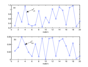
Fig. 1: Profiles of $\sigma_{\epsilon,k}^{2}$ and $\sigma_{\theta,k}^{2}$.

4.1 BG Distribution

The additive noise $v_{k}(i)$ includes the background noise $\theta_{k}(i)$ plus the impulsive noise $\eta_{k}(i)$, where $\theta_{k}(i)$ is zero-mean white Gaussian noise with variance $\sigma_{\theta,k}^{2}$ depicted in Fig. 1(b). The impulsive noise $\eta_{k}(i)$ is described by the BG distribution, $\eta_{k}(i)=b_{k}(i)\cdot g_{k}(i)$, where $b_{k}(i)$ is a Bernoulli process with probability distribution $P[b_{k}(i)=1]=p_{r,k}$ and $\left.P[b_{k}(i)=0]=1-p_{r,k}\right.$, and $g_{k}(i)$ is a zero-mean white Gaussian process with variance $\sigma_{g,k}^{2}$. Here, we set $p_{r,k}$ as a random number in the range of $[0.001,0.05]$, and $\sigma_{g,k}^{2}=1000\sigma_{y,k}^{2}$, where $\sigma_{y,k}^{2}$ denotes the power of $y_{k}(i)=\bm{u}_{k,i}^{T}\bm{w}^{o}$. Fig. 2 compares the performance of the dRLS, dSE-LMS, and RVWC-dLMS algorithms with that of the proposed R-dRLS algorithm. Note that, the R-dRLS (no cooperation) algorithm performs an independent estimation at each node as presented in [25]. For RLS-type algorithms, we choose $\lambda$=0.995 and $\delta$=0.01. As expected, the dRLS algorithm has a poor performance in the presence of impulsive noise. Both the dSE-LMS and RVWC-dLMS algorithms are significantly less sensitive to impulsive noise, but their convergence is slow. Apart from the robustness for combating impulsive noise, the proposed R-dRLS algorithm has also a fast convergence. Moreover, the proposed DNC method can retain the good tracking capability of the R-dRLS algorithm, only with a slight degradation in steady-state performance.

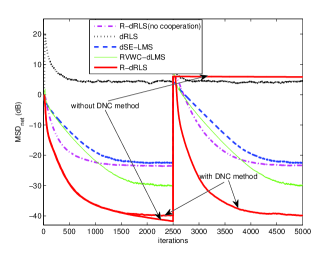
Fig. 2: MSD performance of the algorithms in impulsive noise with BG distribution. Parameter setting of the algorithms (with notations from references) is as follows: $\mu_{k}$=0.015 (dSE-LMS); $\beta$=0.98 and $E_{c}$=1 (R-dRLS); $\varrho$=3 and $t_{th}$=25 (DNC). For the RVWC-dLMS, the Metropolis rule [28] is also used for the combination coefficients in the adaptation step; its other parameters are $L$=16, $\alpha$=2.58, $\lambda$=0.98 and $\mu_{k}$=0.03.

4.2 $\alpha$-Stable Distribution

The impulsive noise is now modeled by the $\alpha$-stable distribution with a characteristic function $\varphi(t)=\exp(-\gamma\lvert t\lvert^{\alpha})$, where the characteristic exponent $\alpha\in(0,2]$ describes the impulsiveness of the noise (smaller $\alpha$ leads to more impulsive noise samples) and $\gamma>0$ represents the dispersion level of the noise. In particular, when $\alpha=2$, it reduces to the Gaussian noise. It is rare to find $\alpha$-stable noise with $\alpha<1$ in practice [27, 46]. In this example, thus we set $\alpha=1.15$ and $\gamma=1/15$. The learning performance of the algorithms is shown in Fig. 3. Fig. 4 shows the node-wise steady-state MSD of the robust algorithms (i.e., excluding the dRLS) against impulsive noise, by averaging over 500 instantaneous MSD values in the steady-state. As can be seen from Figs. 3 and 4, the proposed R-dRLS algorithm with DNC outperforms the known robust algorithms.

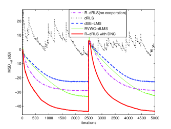
Fig. 3: MSD performance of the algorithms in $\alpha$-Stable noise. Parameter setting is the same as in Fig. 2.

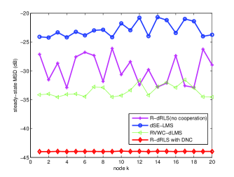
Fig. 4: Node-wise steady-state MSD of the algorithms in $\alpha$-Stable noise.

5 Conclusion

In this paper, the R-dRLS algorithm has been proposed, based on the minimization of an individual RLS cost function with a time-dependent constraint on the squared norm of the intermediate estimate update. The constraint is dynamically adjusted based on the diffusion strategy with the help of side information. The novel algorithm not only is robust against impulsive noise, but also has fast convergence. Furthermore, to track the change of parameters of interest, a detection method (DNC method) is proposed for re-initializing the constraint. Simulation results have verified that the proposed algorithm performs better than known algorithms in impulsive noise scenarios.

References

- [1] A.H. Sayed, “Adaptation, learning, and optimization over networks,” Foundations and Trends in Machine Learning, vol. 7, no. 4-5, pp. 311–801, 2014.
- [2] S. Kanna, D.H. Dini, Y. Xia, S.Y. Hui, and D.P. Mandic, “Distributed widely linear kalman filtering for frequency estimation in power networks,” IEEE Transactions on Signal and Information Processing over Networks, vol. 1, no. 1, pp. 45–57, 2015.
- [3] T.G. Miller, S. Xu, R.C. de Lamare, and H.V. Poor, “Distributed spectrum estimation based on alternating mixed discrete-continuous adaptation,” IEEE Signal Processing Letters, vol. 23, no. 4, pp. 551–555, 2016.
- [4] L. Li, J.A. Chambers, C.G. Lopes, and A.H. Sayed, “Distributed estimation over an adaptive incremental network based on the affine projection algorithm,” IEEE Transactions on Signal Processing, vol. 58, no. 1, pp. 151–164, 2010.
- [5] S.Y. Tu and A.H. Sayed, “Diffusion strategies outperform consensus strategies for distributed estimation over adaptive networks,” IEEE Transactions on Signal Processing, vol. 60, no. 12, pp. 6217–6234, 2012.
- [6] C.G. Lopes and A.H. Sayed, “Diffusion least-mean squares over adaptive networks: Formulation and performance analysis,” IEEE Transactions on Signal Processing, vol. 56, no. 7, pp. 3122–3136, 2008.
- [7] F.S. Cattivelli, C.G. Lopes, and A.H. Sayed, “Diffusion recursive least-squares for distributed estimation over adaptive networks,” IEEE Transactions on Signal Processing, vol. 56, no. 5, pp. 1865–1877, 2008.
- [8] J. Chen and A.H. Sayed, “Diffusion adaptation strategies for distributed optimization and learning over networks,” IEEE Transactions on Signal Processing, vol. 60, no. 8, pp. 4289–4305, 2012.
- [9] S. Xu, R. C. de Lamare, and H. V. Poor, “Distributed estimation over sensor networks based on distributed conjugate gradient strategies,” IET Signal Processing, vol. 10, no. 3, pp. 291–301, 2016.
- [10] H.S. Lee, S.E. Kim, J.W. Lee, and W.J. Song, “A variable step-size diffusion LMS algorithm for distributed estimation.,” IEEE Trans. Signal Processing, vol. 63, no. 7, pp. 1808–1820, 2015.
- [11] S. Xu, R.C de Lamare, and H.V. Poor, “Adaptive link selection algorithms for distributed estimation,” EURASIP Journal on Advances in Signal Processing, vol. 2015, no. 1, pp. 86, 2015.
- [12] S. Xu, R.C de Lamare, and H.V. Poor, “Distributed compressed estimation based on compressive sensing,” IEEE Signal Processing Letters, vol. 22, no. 9, pp. 1311–1315, 2015.
- [13] Z. Liu, Y. Liu, and C. Li, “Distributed sparse recursive least-squares over networks.,” IEEE Trans. Signal Processing, vol. 62, no. 6, pp. 1386–1395, 2014.
- [14] S. Xu, R. C. de Lamare, and H. V. Poor, “Distributed low-rank adaptive estimation algorithms based on alternating optimization,” Signal Processing, vol. 144, pp. 41 – 51, 2018.
- [15] K.L. Blackard, T.S. Rappaport, and C.W. Bostian, “Measurements and models of radio frequency impulsive noise for indoor wireless communications,” IEEE Journal on selected areas in communications, vol. 11, no. 7, pp. 991–1001, 1993.
- [16] J. Ni, J. Chen, and X. Chen, “Diffusion sign-error LMS algorithm: Formulation and stochastic behavior analysis,” Signal Processing, vol. 128, pp. 142–149, 2016.
- [17] D.C. Ahn, J.W. Lee, S.J. Shin, and W.J. Song, “A new robust variable weighting coefficients diffusion LMS algorithm,” Signal Processing, vol. 131, pp. 300–306, 2017.
- [18] S. Al-Sayed, A.M. Zoubir, and A.H. Sayed, “Robust distributed estimation by networked agents,” IEEE Transactions on Signal Processing, vol. 65, no. 15, pp. 3909–3921, Aug. 2017.
- [19] S. Kumar, U.K. Sahoo, A.K. Sahoo, and D.P. Acharya, “Diffusion minimum-wilcoxon-norm over distributed adaptive networks: Formulation and performance analysis,” Digital Signal Processing, vol. 51, pp. 156–169, 2016.
- [20] M. F. Kaloorazi and R. C. de Lamare, “Subspace-orbit randomized decomposition for low-rank matrix approximations,” IEEE Transactions on Signal Processing, vol. 66, no. 16, pp. 4409–4424, Aug 2018.
- [21] M. F. Kaloorazi and R. C. de Lamare, “Compressed randomized utv decompositions for low-rank matrix approximations,” IEEE Journal of Selected Topics in Signal Processing, vol. 12, no. 6, pp. 1155–1169, Dec 2018.
- [22] S. D. Somasundaram, N. H. Parsons, P. Li, and R. C. de Lamare, “Reduced-dimension robust capon beamforming using krylov-subspace techniques,” IEEE Transactions on Aerospace and Electronic Systems, vol. 51, no. 1, pp. 270–289, January 2015.
- [23] H. Ruan and R. C. de Lamare, “Robust adaptive beamforming using a low-complexity shrinkage-based mismatch estimation algorithm,” IEEE Signal Processing Letters, vol. 21, no. 1, pp. 60–64, Jan 2014.
- [24] H. Ruan and R. C. de Lamare, “Robust adaptive beamforming based on low-rank and cross-correlation techniques,” IEEE Transactions on Signal Processing, vol. 64, no. 15, pp. 3919–3932, Aug 2016.
- [25] L.R. Vega, H. Rey, J. Benesty, and S. Tressens, “A fast robust recursive least-squares algorithm,” IEEE Transactions on Signal Processing, vol. 57, no. 3, pp. 1209–1216, 2009.
- [26] A.H. Sayed, Adaptive filters, John Wiley & Sons, 2011.
- [27] K. Pelekanakis and M. Chitre, “Adaptive sparse channel estimation under symmetric alpha-stable noise,” IEEE Transactions on wireless communications, vol. 13, no. 6, pp. 3183–3195, 2014.
- [28] N. Takahashi, I. Yamada, and A.H. Sayed, “Diffusion least-mean squares with adaptive combiners: Formulation and performance analysis,” IEEE Transactions on Signal Processing, vol. 58, no. 9, pp. 4795–4810, 2010.
- [29] I. Song, P.G. Park, and R.W. Newcomb, “A normalized least mean squares algorithm with a step-size scaler against impulsive measurement noise,” IEEE Transactions on Circuits and Systems II: Express Briefs, vol. 60, no. 7, pp. 442–445, 2013.
- [30] Z. Yang, R. C. de Lamare, and X. Li, “-regularized stap algorithms with a generalized sidelobe canceler architecture for airborne radar,” IEEE Transactions on Signal Processing, vol. 60, no. 2, pp. 674–686, Feb 2012.
- [31] J. Hur, I. Song, and P.G. Park, “A variable step-size normalized subband adaptive filter with a step-size scaler against impulsive measurement noise,” IEEE Transactions on Circuits and Systems II: Express Briefs, vol. 64, no. 7, pp. 842–846, 2017.
- [32] R. C. de Lamare and R. Sampaio-Neto, “Adaptive reduced-rank mmse filtering with interpolated fir filters and adaptive interpolators,” IEEE Signal Processing Letters, vol. 12, no. 3, pp. 177–180, March 2005.
- [33] R. C. de Lamare and R. Sampaio-Neto, “Adaptive reduced-rank processing based on joint and iterative interpolation, decimation, and filtering,” IEEE Transactions on Signal Processing, vol. 57, no. 7, pp. 2503–2514, July 2009.
- [34] R. Fa, R. C. de Lamare, and L. Wang, “Reduced-rank stap schemes for airborne radar based on switched joint interpolation, decimation and filtering algorithm,” IEEE Transactions on Signal Processing, vol. 58, no. 8, pp. 4182–4194, Aug 2010.
- [35] R. C. De Lamare and R. Sampaio-Neto, “Minimum mean-squared error iterative successive parallel arbitrated decision feedback detectors for ds-cdma systems,” IEEE Transactions on Communications, vol. 56, no. 5, pp. 778–789, May 2008.
- [36] P. Li, R. C. de Lamare, and R. Fa, “Multiple feedback successive interference cancellation detection for multiuser mimo systems,” IEEE Transactions on Wireless Communications, vol. 10, no. 8, pp. 2434–2439, August 2011.
- [37] R. C. de Lamare, “Adaptive and iterative multi-branch mmse decision feedback detection algorithms for multi-antenna systems,” IEEE Transactions on Wireless Communications, vol. 12, no. 10, pp. 5294–5308, October 2013.
- [38] L.R. Vega, H. Rey, J. Benesty, and S. Tressens, “A new robust variable step-size NLMS algorithm,” IEEE Transactions on Signal Processing, vol. 56, no. 5, pp. 1878–1893, 2008.
- [39] A. G. D. Uchoa, C. Healy, R. C. de Lamare, and R. D. Souza, “Design of ldpc codes based on progressive edge growth techniques for block fading channels,” IEEE Communications Letters, vol. 15, no. 11, pp. 1221–1223, November 2011.
- [40] C. T. Healy and R. C. de Lamare, “Decoder-optimised progressive edge growth algorithms for the design of ldpc codes with low error floors,” IEEE Communications Letters, vol. 16, no. 6, pp. 889–892, June 2012.
- [41] C. T. Healy and R. C. de Lamare, “Design of ldpc codes based on multipath emd strategies for progressive edge growth,” IEEE Transactions on Communications, vol. 64, no. 8, pp. 3208–3219, Aug 2016.
- [42] J. Liu and R. C. de Lamare, “Low-latency reweighted belief propagation decoding for ldpc codes,” IEEE Communications Letters, vol. 16, no. 10, pp. 1660–1663, October 2012.
- [43] C. Healy, Z. Shao, R. M. Oliveira, R. C. d. Lamare, and L. L. Mendes, “Knowledge-aided informed dynamic scheduling for ldpc decoding of short blocks,” IET Communications, vol. 12, no. 9, pp. 1094–1101, 2018.
- [44] S. Chouvardas, K. Slavakis, and S. Theodoridis, “Adaptive robust distributed learning in diffusion sensor networks,” IEEE Transactions on Signal Processing, vol. 59, no. 10, pp. 4692–4707, 2011.
- [45] L. Lu, H. Zhao, and B. Chen, “Improved-variable-forgetting-factor recursive algorithm based on the logarithmic cost for volterra system identification,” IEEE Transactions on Circuits and Systems II: Express Briefs, vol. 63, no. 6, pp. 588–592, 2016.
- [46] M. Shao and C.L. Nikias, “Signal processing with fractional lower order moments: stable processes and their applications,” Proceedings of the IEEE, vol. 81, no. 7, pp. 986–1010, 1993.