HST FUV SPECTROSCOPY OF THE SHORT ORBITAL PERIOD RECURRENT NOVA CI AQL: IMPLICATIONS FOR WHITE DWARF MASS EVOLUTION

Abstract

An HST COS Far UV spectrum (1170 Å to 1800 Å) was obtained for the short orbital period recurrent novae (T Pyxidis subclass), CI Aquilae. CI Aql is the only classical CV known to have two eclipses of sensible depth per orbit cycle and also have pre- and post-outburst light curves that are steady enough to allow estimates of mass and orbital period changes. Our FUV spectral analysis with model accretion disks and NLTE high gravity photospheres, together with the Gaia parallax, reveal CI Aql’s FUV light is dominated by an optically thick accretion disk with an accretion rate of the order of $4\times 10^{-8}$ $M_{\sun}/yr$. Its database of light curves, radial velocity curves, and eclipse timings is among the best for any CV. Its orbit period ($P$), $dP/dt$, and reference time are re-derived via simultaneous analysis of the three data types, giving a dimensionless post-outburst $dP/dt$ of $-2.49\pm 0.95\times 10^{-10}$. Lack of information on loss of orbital to rotational angular momentum leads to some uncertainty in the translation of $dP/dt$ to white dwarf mass change rate, $dM_{1}/dt$, but within the modest range of $+4.8\times 10^{-8}$ to $+7.8\times 10^{-8}$ $M_{\sun}/yr$. The estimated white dwarf mass change through outburst for CI Aql, based on simple differencing of its pre- and post outburst orbit period, is unchanged from the previously published $+5.3\times 10^{-6}M_{\sun}$. At the WD’s estimated mass increase rate, it will terminate as a Type Ia supernova within 10 million years.

1 Introduction: the Short Orbital Period Recurrent Nova CI Aql

Cataclysmic variables (CVs) are close binaries comprised of a main sequence, sub-giant, or giant star that fills its Roche-lobe and transfers gas to a white dwarf (WD) via an accretion disk if the WD is only weakly magnetic or via a magnetically channeled accretion column if the WD is strongly magnetic. When a critical mass of hydrogen-rich gas accumulates on the white dwarf, an explosive thermonuclear runaway(TNR) is triggered, identified as a classical nova. The recurrent novae (RNe) are a subset of CVs that have suffered more than one recorded (TNR) outburst on recurrence timescales of a year to a century. Recent reviews on the properties and basic parameters of RNe can be found in Anupama (2008, 2013) and Schaefer (2010). Their short recurrence times require both a massive WD and a high accretion rate (Starrfield, Sparks, & Truran, 1985; Yaron, et al., 2005). These two conditions are required for an accreting WD to explode as a Type Ia supernova (SN Ia), which is why RNe are among the best possibilities for a solution to the longstanding SN Ia progenitor problem (Pagnotta & Schaefer, 2014).) This single degenerate scenario and the double-degenerate merger scenario (Iben & Tutukov, 1984; Webbink, 1984) both remain viable pathways to SN Ia explosions.

A small subclass of RNe (T Pyx, IM Nor, CI Aql) have short orbital periods (relative to other recurrent novae) and main sequence (MS) donor companions. All other RNe have subgiant or red giant donors and long orbital periods (days to years). The hallmark of these three objects is their slow optical decline timescales compared to other recurrent novae. However, estimates of their ejecta masses, ejection velocities and soft-X-ray runoff times are comparable to other recurrent novae and fast classical novae. This led Caleo & Shore (2015) to propose that their slower optical declines can be explained as gas which is transferred into the Roche lobe of the WD by the donor star in the first few days of the nova explosion, blocking the radiation from ionizing the ejecta and increasing the optical decline timescale. Whether or not this explains their distinctive slow declines requires further exploration.

The accretion disks and accreting white dwarfs in CVs (including RNe) have the peaks of their spectral energy distributions in the FUV and are best studied there. FUV observations can yield accurate accretion rates, and if the WD is exposed, also its surface temperature and possibly its rotation rate and chemical abundances. Due to its faintness, CI Aql had not previously been observed in the far ultraviolet (FUV). Therefore, we requested Hubble Space Telescope (HST) observations of CI Aql with the Cosmic Object Spectrograph (COS) and carried out an analysis of the HST COS FUV spectrum using the parameters in Table 1, including the newly available Gaia distances.

Iijima (2012) showed that CI Aql’s optical spectral evolution during the 2000 outburst resembled those of T Pyx type RNe’s. Lederle & Kimeswenger (2003) (hereafter LK) and Mennickent & Honeycutt (1995) (hereafter MH) found that CI Aql shows eclipses on an orbital period of 14.8 $hr$, with an evolved (MH) or main sequence (LK) donor star. Its optical quiescence spectrum is very different from those of typical quiescent novae. The spectrum shows weak emission lines due to HeII and, in addition, the C III-N III complex on a reddened continuum (Anupama, 2013).

CI Aql was detected as a soft X-ray source 14 and 16 months after the 2000 outburst (Greiner & Di Stefano, 2002). From radial velocities (hereafter RV), Sahman, et al. (2013) found the mass of the WD to be $1.00\pm 0.14M_{\sun}$ and the mass of the donor star to be $2.32\pm 0.19M_{\sun}$ (see Table 1). They estimate the secondary’s radius to be $2.07\pm 0.06$ $R_{\sun}$, implying that it is a slightly evolved early A-type star. The high mass ratio of $M_{2}/M_{1}=q=2.35\pm 0.24$ and the high secondary-star mass implies that the mass transfer occurs on a thermal time-scale. Sahman & Dhillon (2013) suggest that CI Aql may be evolving into a persistent supersoft x-ray source, and may eventually explode as an SN Ia. Models also suggest it may ultimately explode as a SN Ia, possibly within 10 Myr (Sahman, et al., 2013). Moreover, Wilson & Honeycutt (2014) (hereafter WH) found that both the 2000 post-outburst rate of period change, $dP/dt$, and $\Delta M_{1}$ (pre- vs. post-outburst $M_{1}$ change) indicate that the WD is growing in mass.

Whether the white dwarf in a recurrent nova increases or decreases its mass with each nova outburst is key to understanding whether they are progenitors of Type Ia supernovae. Given the critical importance of this question, we extend WH’s analysis of light curves and eclipse timings to include also RV curves and report the results in later sections.

CI Aql’s post-outburst ephemeris ($HJD_{0}$, $P$, $dP/dt$) is derived in §2.1 by simultaneous solution of all light curves, RV curves, and eclipse timings that could be found (See §2 for an overview). The algorithm (Wilson & Van Hamme, 2014) iteratively revises the observational weights to ensure properly balanced influence of the three data types. Eclipse timings can cover otherwise blank epochs, but most CI Aql ephemeris information comes from the light and RV curves. The simultaneous solutions improve the accuracy of $dP/dt$. Then application of eqn. 5 of WH, derived in their §5.1, yields $dM_{1}/dt$ with improved accuracy, after adoption of a plausible range for conversion of orbital to rotational angular momentum. Accretion rates ($dM_{1}/dt$) are derived here from the CI Aql FUV spectrum for the first time and compared with those for T Pyx (Godon, et al., 2018). Disk modeling codes are described and the results summarized in §3.2 and §3.3, respectively, along with implications for this subclass of RNe. We also looked for spectroscopic evidence of wind outflow during quiescence in the form of P Cygni line profiles and blue-shifted absorption features. Spectroscopic detection of the underlying white dwarfs is unlikely, due to the anticipated bright accretion disk. Details of CI Aql HST COS observations are in §3.1.

2 $dP/dt$ and $dM_{1}/dt$ – Making the Most of Timing Data

A central issue regarding the decades-old and currently undecided conjecture that RNe are precursors to SN Ia events is whether the WD typically gains or loses mass over a full nova outburst. Crucial to this point is whether the orbital period, $P$, increases or decreases because of the nova event, although that may not be easy or even possible to decide where the pre-explosion observations are sketchy or absent. Since the WD mass surely decreases in the initial part of the explosion, an overall increase requires substantially positive $dM_{1}/dt$ at a subsequent time before the outburst. One possible mechanism is additional mass accretion during the common envelope stage of the outburst when the white dwarf remains bloated following the dynamical ejection (Sion & Sparks, 2014). Eqn. 5 of WH quantifies how to compute $dM_{1}/dt$ from $dP/dt$ during intervals when there is no mass loss from the system (conservative case).

Traditionally, almost all binary system $dP/dt$ estimates are from eclipse timings, but we apply a relatively new and more accurate technique that needs no timing estimates (Wilson, 2005, 2006; Wilson & Van Hamme, 2014). The traditional way operates in two steps – first measure eclipse times, then fit an ephemeris to the measures. Each step has its own errors. The new way operates directly with original photometry and RVs, allows step 1 to be bypassed, and completely eliminates errors in eclipse time estimates. Although the ephemeris algorithm streamlines the process and does save work, the important advance is in accuracy, by elimination of an error source. The result is a more accurate ephemeris, including a $dP/dt$ term that leads to $dM_{1}/dt$. An important development is that Sahman, et al. (2013) now have RVs of both CI Aql components that have put knowledge of the component star masses on a firm footing. The newly derived masses are very different from those made in the absence of velocity information.

2.1 CI Aql Ephemeris and Masses from Light Curves, Radial Velocities, and Eclipse Timings

Analysis of CI Aql RVs has been carried out by Sahman, et al. (2013) in terms of a traditional point source model, with an intricate multi-step Monte Carlo solution process. The reader is referred to §3.9 of Sahman, et al. (2013) for their step by step strategy and specifics. Our solution is by a differential corrections algorithm ($DC$) that has been optimized in various ways since its initial publication (Wilson & Devinney, 1971), for example, by introduction of simultaneous multi-datatype solutions, three kinds of data weighting, direct distance estimation, and several ways to improve convergence. Light curves, RVs, and eclipse timings exist for CI Aql so combinations of those datatypes can be in the input data stream for simultaneous post-outburst $dP/dt$ computation. With only RVs and eclipse timings as input, 179 Sahman, et al. RVs and 45 Schaefer timings were entered. Insertion of the 1493 light curve points is not a viable option with a point source model since no computed eclipses or proximity effects will match those observed – the computed light curves will be flat. If other than ephemeris parameters are to be measured, then a similar argument can be made against any model that lacks a disk, since the light curves, although not flat, will not correspond to a disk model.

Parameters directly at issue are the mass ratio and orbit size (i.e. $a$, the orbital semi-major axis), since these are determined well from double-lined spectra and jointly produce the individual star masses via Kepler’s Third Law. Those quantities are likely to be corrupted by the light curves in simultaneous light/RV no-disk solutions, as the diskless geometry is wrong for a CV. However the published light curves do have ephemeris information, so the issue becomes – can one tap into that information by inclusion of the light curves without damage to the mass ratio and orbit size results? A modest step in the interest of maximizing ephemeris information via insertion of light curves can be a two part process with the stars made very small (essentially a point source model) and the RV curves and timings solved for parameters [$a$,$M_{2}/M_{1}$]. The light curves are then included with only [$HJD_{0}$, $P_{0}$, $dP/dt$] as output, keeping [$a$,$M_{2}/M_{1}$] fixed. Solutions of this kind with $dP/dt$ adjusted and also fixed at zero were carried out in a few minutes of machine time.

2.2 Slightly Changed Ephemeris and Masses

As we now have the Sahman, et al. RVs, the solution for $P$, $dP/dt$, reference time, and a few other parameters from WH was done again with the RVs as additional input. Results are in Table 2, with non-zero post-eruption $dP/dt$ now a $2.6\sigma$ result compared to the previous $2.4\sigma$ and again with negative sign. The derived post-eruption period is the same as in WH, within its uncertainty. With light curves suppressed, $dP/dt$ was zero within its uncertainty ($+0.9\pm 3.1\times 10^{-10}$), which is not surprising since all RVs were taken within 2 days and lie within the time base of the eclipse timings that produced no measurable $dP/dt$ when analyzed separately. This outcome shows that light curves are not just helpful but necessary at this time for meaningful estimation of $dP/dt$ in CI Aql. $dP/dt$ was assumed to be zero for the solution with light curves omitted.

2.3 The Rate of Post-outburst White Dwarf Mass Change

A mis-typed sign has been noticed in the earlier numerical evaluation by WH of eqn. 5 for $dM_{1}/dt$ (the programmed sign was plus [+] instead of the correct minus [-]), in the term involving $dJ/dM_{1}$. Their Figure 5 thereby needs revision and an erratum will be published. The figure’s purpose was to quantify the effect on ephemeris-based $dM_{1}/dt$ of orbital angular momentum ($J_{orb}$) loss from conversion to rotational angular momentum. Most of the computed $dM_{1}/dt$’s are now somewhat smaller, following this fix, although all remain substantially positive for parameters similar to those of CI Aql and any negative $dP/dt$. Estimated $dM_{1}/dt$ now ranges from $+7.8\times 10^{-8}$ $M_{\sun}/yr$ for negligible loss of orbital angular momentum to rotation, down to $+4.8\times 10^{-8}$ $M_{\sun}/yr$ for maximum plausible loss of $J_{orb}$. The overall result remains that conversion of orbital to rotational angular momentum is not sufficient to call the order of estimated (post-eruption) white dwarf mass accretion rate into question.

2.4 White Dwarf Mass Change Estimation by Simple Period Differencing

WH stress that estimated period change (post-outburst minus pre-outburst, $\Delta P$) accuracy is limited by uncertainty in pre-outburst $P$, due to a relatively unpopulated pre-outburst database. That is still true since we have no new pre-outburst observations. Addition of RVs to the input stream did not significantly change the post outburst period. With no further post-outburst data except for the Sahman, et al. (2013) RVs, $\Delta P$’s estimated value remains as in WH, again being $-2.0\pm 1.4\times 10^{-6}$ days. $\Delta M_{1}$ also is unchanged at $+5.3\pm 3.7\times 10^{-6}M_{\sun}$, as it scales with $\Delta P$ while the other relevant parameters are nearly the same as before. Although this $\Delta M_{1}$ result differs from zero by only $1.4\sigma$, the pre- and post-outburst periods upon which it is based are respectively from well before and well after the outburst of early 2000, so they have as much independence from outburst-induced light curve disturbances as existing data can provide. A set of lightcurves over an interval of about one year in 2001/2002 is illustrated in LK’s Fig. 8. They estimated from overall system brightness that CI Aql’s return to quiescence following the 2000 outburst occurred in February/March, 2002. Since the 2001/2002 observations have a short time base of only 13 months, lie mostly or entirely within the disturbed interval following outburst, and show much larger asymmetries than those of pre- or post-outburst times, we shall not attempt to fit them into the overall picture. LK also utilized pre-outburst photometric coverage from 1991 to 1996 (conveyed by R.K Honeycutt prior to publication), from which they estimated CI Aql’s pre-outburst $P_{orb}$ to be $0.6183609\pm 0.0000009$ by the phase dispersion minimization (PDM) algorthm (Stellingwerf, 1978). This period may seem to differ considerably from that measured by WH from the same data but the difference is only about half of the rather large statistical uncertainty.

3 Spectral Analysis

3.1 HST COS Observation of CI Aql

The HST COS spectrum of CI Aql was obtained on November 2, 2017 at 6:36 UT with an exposure time 6198.816 s in TIME-TAG mode with the G140L disperser centered at 1105 Å (segment B is turned off) through the PSA aperture configured to COS/FUV. The COS G140L grating covers a wider wavelength range than STIS G140L so our spectra have about 2.5 times better resolution than STIS. The COS spectrum extends from 1121 Å to 2148 Å. However, due to low S/N at the edges of the segment, we ignore the regions shorter than 1150 Å and longer than 1900 Å.

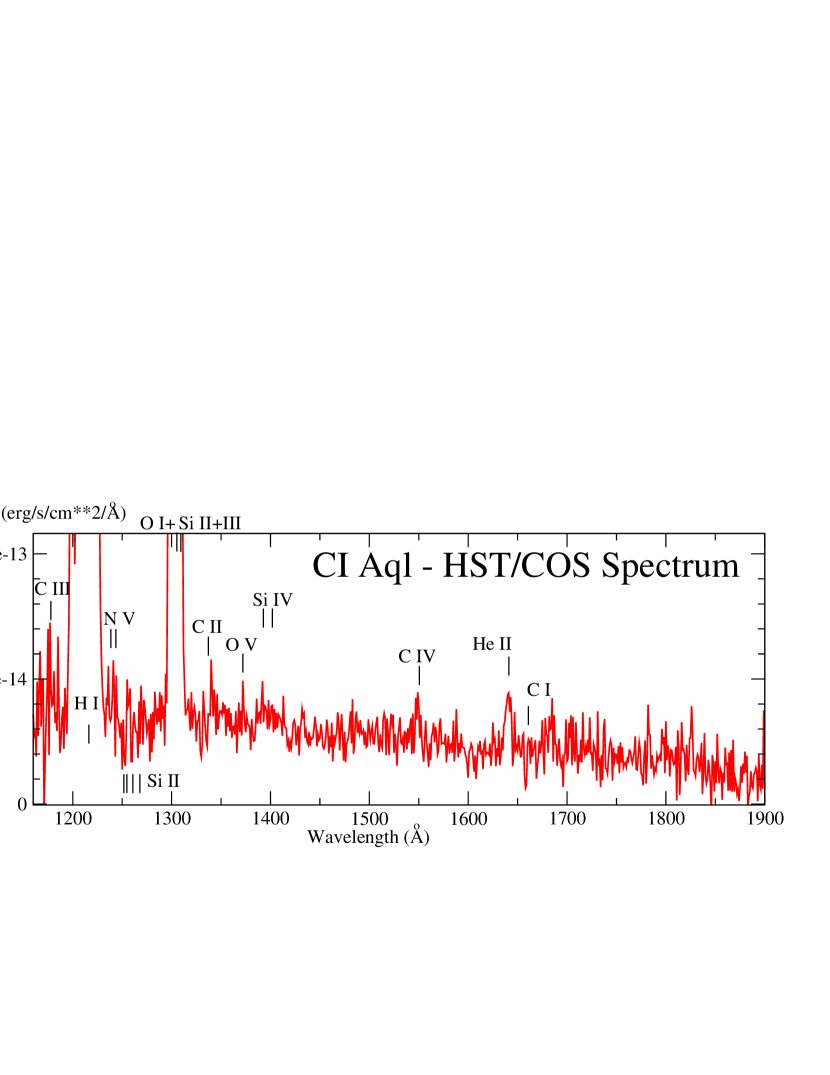
Figure 1: The HST COS spectrum of CI Aql with the strongest line features identified. Strong emission is seen due to $Ly_{\alpha}$ and strong O i + Si iii (1300A). Relatively weak emission features appear due to C iii (1175), N v (1238, 1242), C ii, (1335), Si iv (1394, 1402), O v(1371), C iv (1548, 1550), He ii (1640), and Al II (1670).

Fig. 1 shows the CI Aql spectrum, with a strong continuum that rises toward shorter wavelengths. The strongest emission lines are $Ly_{\alpha}$ and O i + Si iii (1300 Å). Weaker emission lines are seen due to C iii (1175 Å), C iv (1550 Å), He ii (1640 Å), Al ii (1670 Å), and weak O v (1371 Å).

3.2 Theoretical Disk and Photosphere Models

We use the suite of codes TLUSTY, SYNSPEC and DISKSYN (Hubeny, 1988; Hubeny & Lanz, 1995), for constructing grids of accretion disk models and NLTE high gravity photosphere models. Our disk models, including non-standard disks, are described in Godon, et al. (2017). We also adopted model accretion disks from the grid of solar composition optically thick, steady state disk models (“the standard disk model”) of Wade & Hubeny (1998). In these accretion disk models, the outermost disk radius, $R_{\rm out}$, is chosen so that $T_{\rm eff}$ ($R_{\rm out}$) is near 10,000K since disk annuli beyond this point, which are cooler zones with larger radii, would provide only a very small contribution to the mid and far UV disk flux. For the disk models, unless otherwise specified, we selected every combination of $\dot{M}$, inclination, and white dwarf mass to fit the data: the inclination angle i = 18, 41, 60, 75 and 81 degrees, $M_{\rm wd}$ = 0.80, 1.03, 1.21 $M_{\odot}$ and $\log(\dot{M})$ ($M_{\odot}$/yr) = -8.5, -9.0, -9.5, -10.0, -10.5. For the WD models, we constructed solar composition WD stellar photospheres with temperatures from 12,000 K to 60,000 K in steps of 1,000K to 5,000 K, and with effective surface gravity corresponding to the WD mass of the accretion disk model. We adopt a projected rotation rate $V_{\rm rot}\sin(i)$ of 200 km/s. We carried out synthetic spectral fitting with a combination of disks and photospheres to model the HST spectra.

The fitting errors are mainly due to uncertainties in the WD mass, $M_{\rm wd}$, and distance, $d$. Similar errors (5-10% in $T_{eff}$ , $\approx$ 0.5 in log(g)) are obtained if either $M_{\rm wd}$ or $d$ are completely unknown. For accretion disk spectral fits, if either $d$ or $M_{\rm wd}$ is unknown, then the errors in $log(\dot{M})$ can be as large as $\approx 1$ (in units of $\dot{M}$/yr, namely e.g. $log(\dot{M})=-9\pm 1$ ) for a COS spectrum. If the $M_{\rm wd}$ and $d$ are known, a high S/N COS spectrum will have errors of barely 100 K in $T_{eff}$ (for a WD fit), or $\approx 0.2$ in $log(\dot{M})$ (e.g. $\log(\dot{M})=-9.0\pm 0.2$).

Simple inversion of a Gaia parallax can provide an acceptable distance only when a precise parallax for an individual object is used (Luri, et al., 2018). Uncertainties are typically around 0.04 mas for Gaia sources brighter than $\sim$14 mag, around 0.1 mas for sources with a G magnitude around 17, and around 0.7 mas at the faint end, around 20 mag. Irregular color and brightness changes introduce uncertainties and must be monitored. Gaia Data Release 1 parallaxes proved successful for virtually all of the test case CVs and the old nova RR Pic. SS Cygni’s distance of $\approx$ 114 $pc$ for the disk instability model to be valid was solidly confirmed with a Gaia parallax distance of 117 $pc$ (Ramsay, et al., 2017).

Schaefer (Schaefer, 2018) has concluded a study of the GAIA parallaxes of classical novae and recurrent novae in which he assesses the reliability of the distance for each object. He ranks the GAIA results for CI Aql and T Pyx in his ”gold” category meaning the highest level of reliability.

3.3 FUV Spectroscopic Modeling

We carried out CI Aql accretion disk fits scaled to the Gaia distance of 3.062 kpc for the WD mass reported in §2 of 0.996 $M_{\sun}$, with LK’s inclination of $71^{\circ}$. $E_{B-V}$ was set to 0.8 although values as large as 0.98 appear in the literature. We constructed disk models from scratch with fixed dimensions. The inner disk radius was taken to be 5200 km while the outer disk radius, Rd, was chosen such that the outer disk’s surface temperature reaches only 5,000 K so its contribution to the FUV is insignificant. This best fit yields an accretion rate of $dM/dt=4\times 10^{-8}M_{\sun}/yr$, and its spectrum is displayed in Fig. 2. We examined the possibility that a hot white dwarf could be contributing FUV flux, but its radius and surface temperature would have to be untenably large to provide the observed flux at a distance of 3 kpc.

4 Discussion & Conclusions

We have characterized FUV spectrum of the key RNe, CI Aql. For CI Aql, with a Gaia distance of 3.062 kpc, an accretion disk model satisfying the new distance yields an accretion rate $4\times 10^{-8}M_{\sun}/yr$ for $M_{\rm wd}=1.0M_{\sun}$, with a white dwarf radius of 5200 km.

Shara, et al. (2015) derived WD masses and accretion rates for all of the known recurrent novae from relationships between WD masses and accretion rates versus nova characteristics such as observed outburst amplitudes, decline times, and envelope masses. Their grids of multicycle nova evolution cover a wide range of accretion rates and white dwarf masses. Their white dwarf masses and accretion rates are, for T Pyx, 1.23 $M_{\sun}$, 1.12 $\times 10^{-7}M_{\sun}$/yr; for IM Nor, 1.21 $M_{\sun}$, 4.8 $\times 10^{-8}M_{\sun}$/yr; and for CI Aql, 1.21 $M_{\sun}$, 1.12 $\times 10^{-7}$ $M_{\sun}$/yr. By comparison, Godon, et al. (2018) derived $\dot{M}\sim 10^{-7}$ $M_{\sun}$/yr and $M_{\rm wd}=1.2M_{\sun}$ for T Pyx, which is in good agreement. For CI Aql we derived 4 $\times 10^{-8}M_{\sun}$/yr, which is nearly a factor of three smaller than Shara, et al. (2015).

WH found the WD in CI Aql to show a marginally significant net mass gain, $\Delta M_{1}$, over its full outburst and recovery, via simultaneous solution of light curves and eclipse timings for ephemeris quantities and our revisit of CI Aql finds the same pre- vs. post outburst $\Delta M_{1}$ as in WH, with RVs from double-lined spectra added to the database. $\Delta M_{1}$’s accuracy continues to be set entirely by the less numerous pre-outburst data. If the pre-outburst uncertainty in orbit period ($1.4\times 10^{-6}$ days) had been as small as its post-outburst uncertainty ($9.4\times 10^{-8}$ days), $\Delta P$’s overall standard error would have been about 20 times smaller, as would that of $\Delta M_{1}$, which scales with $\Delta P$. The next outburst should produce more definitive results if followed intensively.

For T Pyx, prototype of the short period RNe subclass, Patterson, et al. (2014) found the WD to be losing mass because the ejected mass exceeds the accreted mass over the time between outbursts ($\Delta t_{ob}$), with accreted mass estimated as $dM_{1}/dt$ $\times$ $\Delta t_{ob}$. Contrasting observational and astrophysical circumstances between T Pyx and CI Aql suggest caution in making comparisons. For example, T Pyx’s light curve data (Patterson, et al., 2014) are much more numerous than CI Aql’s and better distributed in time in regard to pre- and post-outburst coverage. These points lead to a very strong $dP/dt$ measurement for T Pyx (the basis for Patterson, et al. (2014)’s $dM_{1}/dt$ estimate) rather than our consistently negative but only $2.6\sigma$ $dP/dt$ result for CI Aql. That CI Aql’s $dP/dt$ could be measured at all, after previous attempts had failed, is due to the enhanced accuracy of the ephemeris-measuring algorithm applied by WH and in this paper’s §2. Note that the T Pyx masses – especially that of the lobe-filling donor star – differ greatly from those of CI Aql, and the system dimensions are also very different, thus complicating the comparison.

For CI Aql’s WD to have gained mass through its recent eruption event would require large-scale and nearly impulsive accretion when its $dP/dt$ was not measured, some time within the overall outburst process. However that interval is when light curves are disturbed so that measurements of $P$ and corresponding white dwarf mass estimates are unreliable. Given these considerations, we regard the simple period differencing (pre- vs. post outburst) of §2.4 as the preferred way to estimate $\Delta M_{1}$ where suitable data exist. Notably the sign of CI Aql’s $\Delta M_{1}$ has been positive in all of our computations. Note that the WD masses of both IM Nor and CI Aql are far larger than the canonical single white dwarf mass of $0.6M_{\odot}$. This fact in itself suggests that the WD in CI Aql may be growing mass. Whether all, some, or none of the WDs in short period RNe are expected to produce SN Ia’s remains an active issue. With only three such systems now known, the score is tied at 1 to 1 in regard to conclusions for and against these rare objects heading toward an ultimate catastrophe.

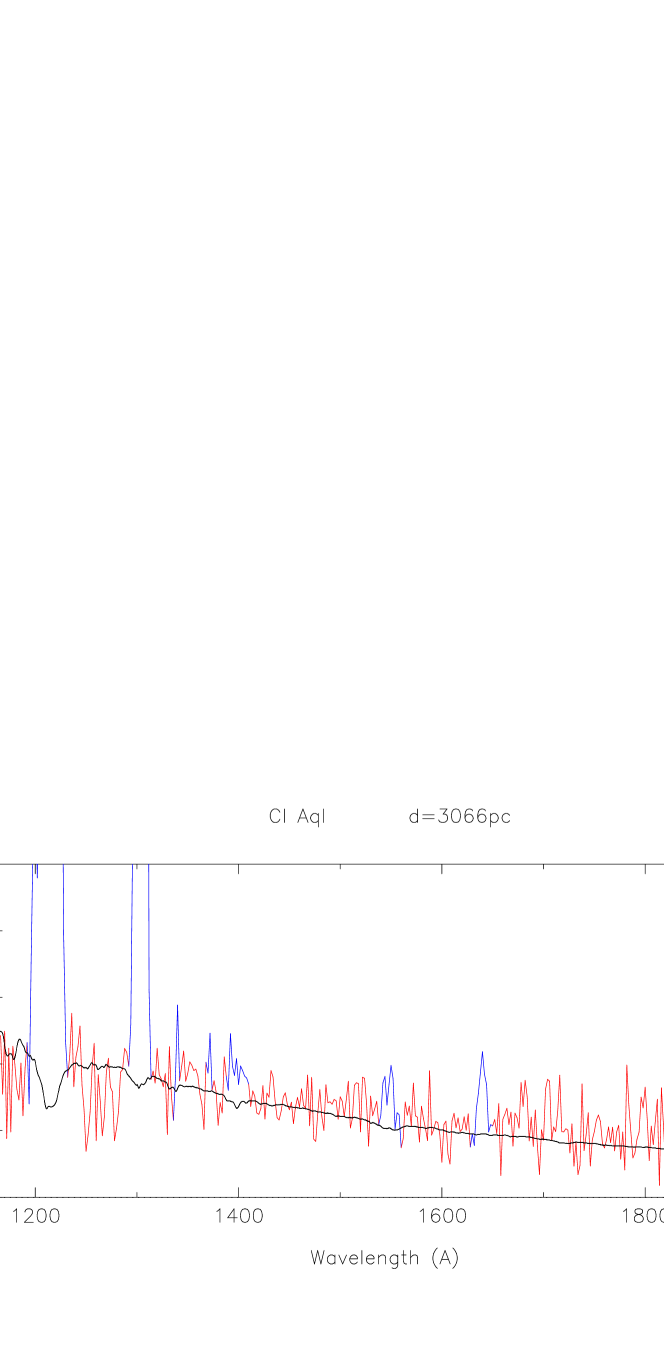
Figure 2: An accretion disk model fit to CI Aql with inner truncation. The inner disk radius was taken to be 5200 km. The outer disk radius, Rd, was chosen such that the outer disk’s surface temperature reaches only 5,000 $K$ so its contribution to the FUV is insignificant. This best fit truncated disk has an accretion rate of $dM/dt=4\times 10^{-8}M_{\sun}/yr$

.

Table 1: Basic Observed Parameters of CI Aql

$V_{max}$	$V_{min}$	$t_{3}$	$P_{orb}$ $(days)$	$E_{B-V}$	$i$	$M_{\rm wd}$ $(M_{\odot})$	$d$ $(kpc)$	Nova Outbursts
9.0	16.7	32	0.62	0.8	71 deg	0.98 $M_{\sun}$	3.06	1917, 1941, 2000

Note. — Item $t_{3}$ is the time in days past peak light for brightness to drop by $3^{m}$.

Table 2: CI Aql Post-outburst Simultaneous Light-RV-Timing Solutions

Parameter	RV & Timing Input	RV, light curve, & Timing Input
$a$ ($R_{\sun}$)	$4.583\pm 0.088$	$4.583$
$V_{\gamma}$ $(km\,s^{-1})$	$+10.3\pm 2.7$	$+10.3$
$m_{2}/m_{1}$	$2.39\pm 0.13$	$2.39$
$HJD_{0}$	$2453652.75826\pm 0.00026$	$2453652.75821\pm 0.00018$
$P_{0}$	$0.61836041\pm 0.00000012$	$0.618360142\pm 0.000000094$
$dP/dt$	$0.00$	$-2.49\pm 0.9510^{-10}$
$M_{1}/M_{\sun}$	$0.996$	…
$M_{2}/M_{\sun}$	$2.38$	…
$R_{2}/R_{\sun}$	$2.10$	…

Note. — Quantities in the last column without standard errors were adopted from the middle column. The orbital inclination was $69^{\circ}$ in all solutions. The mean donor star radius, $R_{2}/R_{\sun}$, follows from the lobe filling condition for synchronous rotation. The middle column’s $dP/dt$ is reported as zero since deletion of light curve input left $dP/dt$ non-significant.

References

- Anupama (2008) Anupama, G.C. 2008, ASPC, 401, 31
- Anupama (2013) Anupama, G.C. 2013, in Binary Paths to Type Ia Supernovae Explosions, Proceedings of the International Astronomical Union, IAU Symposium, Volume 281, p. 154-161
- Caleo & Shore (2015) Caleo, A, & Shore, S. N. 2015, MNRAS, 449, 25
- Godon, et al. (2017) Godon, P., Sion, E.M., Balman, S. Blair, W.P. 2017, ApJ, 846, 52
- Godon, et al. (2018) Godon, P., Sion, E.M., Williams, R.E., & Starrfield, S. 2018, ApJ, 862, 89
- Greiner & Di Stefano (2002) Greiner, J. & Di Stefano, R. 2002, ApJ, 578, L59
- Hubeny (1988) Hubeny, I. 1988, Comp. Phys. Comm., 52, 103
- Hubeny & Lanz (1995) Hubeny, I. & Lanz, T. 1995, ApJ, 439, 875
- Iben & Tutukov (1984) Iben I., Jr, Tutukov A. V., 1984, ApJS, 54, 335
- Iijima (2012) Iijima, T. 2012, A&A, 544, 26
- Lederle & Kimeswenger (2003) Lederle, C. & Kimeswenger, S. 2003, A&A, 397, 951 (LK)
- Luri, et al. (2018) Luri, X., et al. 2018, A&A, Special Gaia Issue)
- Mennickent & Honeycutt (1995) Mennickent, R.E, & Honeycutt, R. K. 1995, IBVS, 4232, 1
- Pagnotta & Schaefer (2014) Pagnotta, A. & Schaefer, B.E. 2014, ApJ, 788, 164
- Patterson, et al. (2014) Patterson, J. et al. 2014, ASPC, 490, 35
- Ramsay, et al. (2017) Ramsay, G., Schreiber, M.R., Gansicke, B.T., & Wheatley, P.J. 2017, A&A, 604, 107
- Sahman & Dhillon (2013) Sahman, D. I. & Dhillon, V. S. 2013, in Binary Paths to Type Ia Supernovae Explosions, IAUS, 281, 193
- Sahman, et al. (2013) Sahman, D. I., Dhillon, V. S., Marsh, T. R., Moll, S., Thoroughgood, T. D., Watson, C. A., & Littlefair, S. P. 2013, MNRAS, 433, 1588
- Schaefer (2010) Schaefer, B. E. 2010, ApJS, 187, 275
- Schaefer (2011) Schaefer, B. E. 2011, ApJ, 742, i2
- Schaefer (2018) Schaefer, B. E. 2018, MNRAS, in press (2018arXiv180900180)
- Shara, et al. (2015) Shara, M. M., Prialnik, D., Hillman, Y., & Kovetz, A. 2015, ApJ, 860, 110
- Sion & Sparks (2014) Sion, E. M. & Sparks, W., ApJ, 796, L10
- Starrfield, Sparks, & Truran (1985) Starrfield, S., Sparks, W. M., & Truran, J. W. 1985, ApJ, 291, 136
- Stellingwerf (1978) Stellingwerf, R.F., ApJ, 224, 953
- Wade & Hubeny (1998) Wade, R.A., & Hubeny, I. 1998, ApJ, 509, 350
- Webbink (1984) Webbink, R.1984, ApJ, 277, 355
- Wilson (2005) Wilson, R. E. 2005, Ap&SS, 296, 197
- Wilson (2006) Wilson, R. E. 2006, ASPC, 349, 71
- Wilson & Devinney (1971) Wilson, R. E. & Devinney, E. J. 1971, ApJ, 166, 605
- Wilson & Van Hamme (2014) Wilson, R. E. & Van Hamme, W. 2014, ApJ, 780, 151
- Wilson & Honeycutt (2014) Wilson, R. E. & Honeycutt, R. K. 2014, ApJ, 795, 8 (WH)
- Yaron, et al. (2005) Yaron, O., Prialnik, D., Shara, M. M., & Kovetz, A. 2005, ApJ, 623, 398
.