Mixed-Order Spectral Clustering for Networks

Abstract

Clustering is fundamental for gaining insights from complex networks, and spectral clustering (SC) is a popular approach. Conventional SC focuses on second-order structures (e.g., edges connecting two nodes) without direct consideration of higher-order structures (e.g., triangles and cliques). This has motivated SC extensions that directly consider higher-order structures. However, both approaches are limited to considering a single order. This paper proposes a new Mixed-Order Spectral Clustering (MOSC) approach to model both second-order and third-order structures simultaneously, with two MOSC methods developed based on Graph Laplacian (GL) and Random Walks (RW). MOSC-GL combines edge and triangle adjacency matrices, with theoretical performance guarantee. MOSC-RW combines first-order and second-order random walks for a probabilistic interpretation. We automatically determine the mixing parameter based on cut criteria or triangle density, and construct new structure-aware error metrics for performance evaluation. Experiments on real-world networks show 1) the superior performance of two MOSC methods over existing SC methods, 2) the effectiveness of the mixing parameter determination strategy, and 3) insights offered by the structure-aware error metrics.

I Introduction

Networks (a.k.a. graphs) are important data structures that abstract relations between discrete objects, such as social networks and brain networks [1]. A network is composed of nodes and edges representing node interactions. Clustering is an important and powerful tool in analysing network data, e.g., for community detection [2, 3, 4, 5, 6].

Clustering aims to divide the data set into clusters (or communities) such that the nodes assigned to a particular cluster are similar or well connected in some predefined sense [7, 8, 9, 10, 11]. It helps us reveal functional groups hidden in data. As a popular clustering method, conventional spectral clustering (SC) [12, 13] encodes pairwise similarity into an adjacency matrix. Such encoding inherently restricts SC to second-order structures [1], such as undirected or directed edges connecting two nodes. However, in many real-world networks, the minimal and functional structural unit of a network is not a simple edge but a small network subgraph (a.k.a. motif) that involves more than two nodes [16], which we call a higher-order structure.

Higher-order structures consist of at least three nodes (e.g., triangles, $4$-vertex cliques) [1]. It can directly capture interaction among three or more nodes. When clustering networks, higher-order structures can be regarded as fundamental units and algorithms can be designed to minimise cutting them in partitioning. Clustering based on higher-order structures can help us gain new insights and significantly improve our understanding of underlying networks. For example, triangular structures, with three reciprocated edges connecting three nodes, play important roles in brain networks [17] and social networks [18, 19]. More importantly, higher-order structures allow for more flexible modelling. For instance, considering directions of edges, there exist $13$ different third-order structures, but only two different second-order structures [20]. Thus, the application can drive which third-order structures to be preserved.

Thus, there are emerging interests in directly modelling higher-order structures in network clustering. These works can be grouped into four approaches: 1) The first approach constructs an affinity tensor to encode higher-order structures and then reduces it to a matrix [21, 22], followed by conventional SC [13]. These methods, such as tensor trace maximisation (TTM) [23], are developed in a closely related problem of hypergraph clustering that considers “hyperedges” connecting multiple nodes. 2) The second approach develops higher-order SC by constructing a transition tensor based on random walks model and then reduces it to a matrix for conventional SC, such as tensor spectral clustering (TSC) [14, 24]. 3) The third approach uses a counting and reweighting scheme to capture higher-order structures and reveal clusters [25], such as motif-based SC (MSC) [1]. 4) The fourth approach is higher-order local clustering aiming to reduce computation cost [26], such as High-Order Structure Preserving Local Clustering (HOSPLOC) [15].

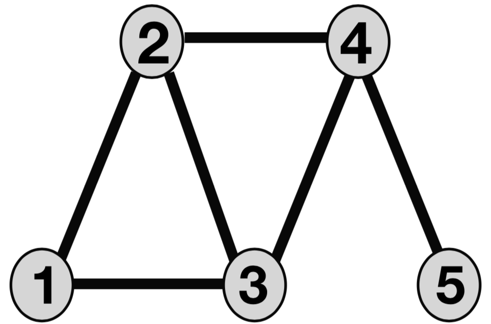
(a) A network.

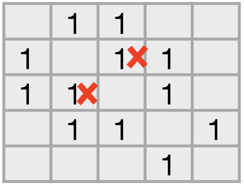
(b) Edges.

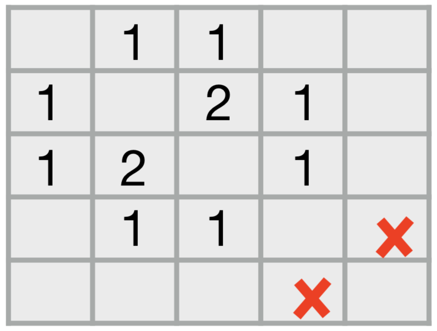
(c) Triangles.

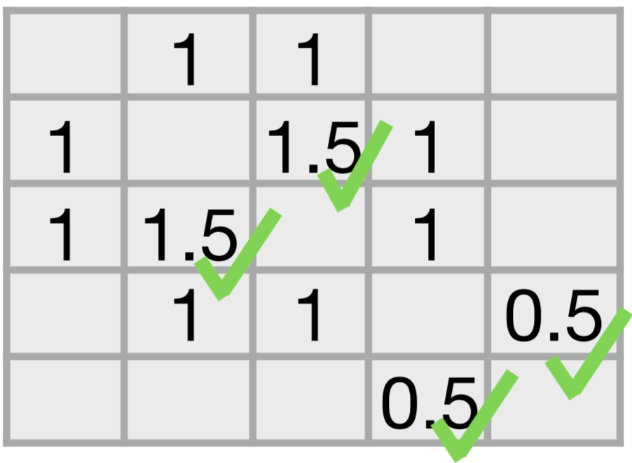
(d) Mixed.

Figure 1: The second and third order structures in (a) can not be fully captured by edge/triangle adjacency matrix in (b)/(c). A mixed adjacency matrix in (d) can capture both.

However, it should be noted that most networks have both second-order and higher-order structures, e.g., the network in Fig. 1(a), and both can be important. Existing conventional and third-order SC methods model only either second-order or third-order structures, but not both, as shown in Figs. 1(b) and 1(c), which fail to properly model the importance between nodes 2 and 3, and nodes 4 and 5, respectively. In Figs. 1(b) and 1(c), each entry indicates the number of edges and triangles involving two nodes of Fig. 1(a).

In this paper, we propose a new Mixed-Order Spectral Clustering (MOSC) to preserve structures of different orders simultaneously, as in Fig. 1(d). For clear and compact presentation, we focus on two undirected unweighted structures: edges (second-order structures) and triangles (third-order structures). Further extensions can be developed for mixing more than two orders, and/or orders higher than three.

We summarise our four contributions as following:

1. Mixed-order models. We develop two MOSC models: one based on Graph Laplacian (GL) and the other based on Random Walks (RW). MOSC-GL combines edge and triangle adjacency matrices to define a mixed-order Laplacian, with its theoretical performance guarantee derived by proving a mixed-order Cheeger inequality. MOSC-RW combines first-order and second-order RW models for a probabilistic interpretation. The final clusters are obtained via a sweep cut procedure or $k$-means. See Sec. III-A and Sec. III-B.

2. Automatic model selection. There is only one hyperparameter in MOSC, i.e., the mixing parameter (ranging from 0 to 1). We propose cut-criteria-based and triangle-density-based strategies to automatically determine the best mixing parameter. See Sec. III-D.

3. Structure-aware error metrics. Existing works on higher-order structure clustering use evaluation metrics focused on mis-clustered nodes [25, 26, 23]. However, mis-clustered nodes do not have a monotonic relationship with mis-clustered structures so they may fail to reflect the errors in structures. Therefore, we propose structure-aware error metrics to gain insights on the quality of structure preservation. See Sec. III-E.

4. Cut criterion. A cut criterion evaluates the quality of output clusters. Therefore, we study seven different sweep cut criteria (both second and third orders) and propose a new one by defining mixed-order conductance. We also propose an optimal cut to study the lower bound of error metrics and model quality. See Secs. IV-B and IV-D.

II Preliminaries

II-A Notations

We denote scalars by lowercase letters, e.g., $a$, vectors by lowercase boldface letters, e.g., $\mathbf{a}$, matrices by uppercase boldface, e.g., $\mathbf{A}$, and tensors by calligraphic letters, e.g., $\mathcal{A}$. Let $\emph{G}=(\emph{V},\emph{E})$ be an undirected unweighted graph (network) with V = {v₁, v₂, …, v_n} being the set of $n$ vertices (nodes), i.e., $n$ = $|\emph{V}|$, and E being the set of edges connecting two vertices.

II-B Normalised Graph Laplacian

Let $\mathbf{W}\in\mathbb{R}^{n\times n}$ be an unweighted adjacency matrix of G where $\mathbf{W}(i,j)$ = 1 if (v_i, v_j) $\in\emph{E}$, otherwise $\mathbf{W}(i,j)$ = 0. The degree matrix $\mathbf{D}$ is a diagonal matrix with diagonal entries $\mathbf{D}(i,i)=\sum_{j=1}^{n}\mathbf{W}(i,j)$, which is the degree of vertex v_i. Let $\mathbf{N}=\mathbf{D}-\mathbf{W}$ denote the Laplacian matrix of $G$. The normalised Laplacian of $G$ is defined as:

$$\mathbf{{L}}=\mathbf{D}^{-\frac{1}{2}}\mathbf{N}\mathbf{D}^{-\frac{1}{2}}.$$ (1)

Let $\mathbf{W}_{T}$ be triangle adjacency matrix of G with its entry ($i$, $j$) being the number of triangles containing vertices $i$ and $j$, which leads to a corresponding weighted graph $G_{T}$ [1]. Similarly, we can define the triangle Laplacian as $\mathbf{N}_{T}=\mathbf{D}_{T}-\mathbf{W}_{T}$ and the normalised triangle Laplacian as:

$$\mathbf{{L}}_{T}=\mathbf{D}_{T}^{-\frac{1}{2}}\mathbf{N}_{T}\mathbf{D}_{T}^{-\frac{1}{2}},$$ (2)

where $\mathbf{D}_{T}(i,i)=\sum^{n}_{j=1}\mathbf{W}_{T}(i,j)$.

II-C First-Order Random Walks for Second-Order Structures

We define a second-order transition matrix $\mathbf{P}$ by normalising the adjacency matrix $\mathbf{W}$ to represent edge structures as [12]:

$$\mathbf{P}=\mathbf{D}^{-1}\mathbf{W}.$$ (3)

The entry $\mathbf{P}_{ij}$ represents the probability of jumping from vertex v_i to v_j in one step. The transition matrix $\mathbf{P}$ represents a random walk process on graph G[12]. From random walk perspective, SC can be interpreted as trying to find a partition of the graph such that the random walk stays long within the same cluster and seldom jumps between clusters [27].

II-D Second-Order Random Walks for Third-Order Structures

Benson et al. [14] extend the above using a three-dimensional transition tensor to encode triangle structures. They firstly define a symmetric adjacency tensor $\mathcal{T}\in\mathbb{R}^{n\times n\times n}$ such that the connectivity information for three vertices {v_i, v_j, v_k}$\in\emph{V}$ can be represented explicitly in this tensor. All entries in $\mathcal{T}$ with a permutation of indices $i$, $j$, $k$ have the same value (hence symmetric). Thus, $\mathcal{T}$ encodes triangle structures in G as:

$$\mathcal{T}(i,j,k)=\left\{\begin{aligned} 1&&\textrm{$v_{i},v_{j},v_{k}$ form a triangle,}\\ 0&&\textrm{otherwise.}\end{aligned}\right.$$ (4)

Next, they form a third-order transition tensor $\mathcal{P}$ as:

$$\mathcal{P}(i,j,k)=\mathcal{T}(i,j,k)/\sum_{m=1}^{n}\mathcal{T}(i,m,k),$$ (5)

where $\sum_{m=1}^{n}\mathcal{T}(i,m,k)\neq$ 0, and 1 $\leq$ $i$, $j$, $k$ $\leq$ $n$. For $\sum_{m=1}^{n}\mathcal{T}(i,m,k)=$ 0, Benson et al. [14] set $\mathcal{P}(i,j,k)$ to $\frac{1}{n}$.

Here, the entries of $\mathcal{P}$ represent the transition probabilities of the second-order random walks. Each vertex in V is considered a distinguishable state. And probability of jumping to state $i$ relies on the last two states $j$ and $k$[28]. This probabilistic interpretation implies that random walks uniformly choose state $i$ that forms a triangle with $j$ and $k$. However, analysing $\mathcal{P}$ is challenging, e.g., finding its eigenvectors is NP-hard [29], so it is often reduced to a similarity matrix to apply conventional SC procedures [14].

II-E Spectral Clustering Basics

Bi-partitioning SC (Algorithm 1) first constructs a matrix $\mathbf{B}$ to encode structures in the input graph G. It then computes a dominant eigenvector $\mathbf{v}$ of $\mathbf{B}$, thus making use of its spectrum. Each entry of $\mathbf{v}$ corresponds to a vertex. Next, we sort vertices by the values $\mathbf{v}(i)$ (or appropriately normalised values) and consider the set $T_{u}$ consisting of the first $u$ vertices in the sorted list, for each $1\leq u\leq n-1$. Then the algorithm finds $S=\arg\min_{T_{u}}\tau(T_{u})$, called the sweep cut w.r.t. some cut criterion $\tau$. Table I lists eight cut criteria, both second and third orders (edge and triangle based). We omit $G$ in the criterion notation $\tau(S;G)$ in the table.

Matrix $\mathbf{B}$ is a crucial part of SC. Conventional (i.e., second-order) SC starts with the adjacency matrix $\mathbf{W}$ of G encoding edges (as in Fig. 1(b)) and defines $\mathbf{B}$ as $\mathbf{W}$, the Laplacian matrix, or their normalised versions [8]. Third-order SC typically starts with a third-order tensor $\mathcal{T}$ encoding triangles, which can be reduced to a matrix $\mathbf{B}$ (as in Fig. 1(c)) to apply Algorithm 1.

Algorithm 1 Bi-partitioning Spectral Clustering

1:  Matrix $\mathbf{B}$ encodes structures of the input graph G.

2:  Compute a dominant eigenvector $\mathbf{v}$ of $\mathbf{B}$.

3:  $\mathbf{v}\leftarrow$ sorted ordering of $\mathbf{v}$ or a normalised version of $\mathbf{v}$.

4:  {$S$, $\bar{S}$} $\leftarrow$ sweep cut of $\mathbf{v}$ w.r.t. some cut criteria.

TABLE I: Edge-based and triangle-based cut criteria.

	Edge-based cuts	Triangle-based cuts
Conductance (${\phi}$)	${\phi_{2}}$($S$) = $\frac{cut_{2}(S)}{\min(vol_{2}(S),vol_{2}(\bar{S}))}$ [8]	$\phi_{3}$($S$) = $\frac{cut_{3}(S)}{\min(vol_{3}(S),vol_{3}(\bar{S}))}$ [14]
Ncut (${\eta}$)	${\eta_{2}}(S)=$$cut_{2}(S)(\frac{1}{{vol_{2}(S)}}+\frac{1}{vol_{2}({\bar{S})}})$ [30]	${\eta_{3}}(S)$ = $cut_{3}(S)(\frac{1}{{vol_{3}({S})}}+\frac{1}{vol_{3}(\bar{S})})$ [31]
Nassoc (${\xi}$)	${\xi_{2}}({S})$ = $\frac{assoc_{2}(S)}{vol_{2}(S)}+\frac{assoc_{2}(\bar{S})}{vol_{2}(\bar{S})}$[30]	${\xi_{3}}({S})=$$\frac{assoc_{3}(S)}{vol_{3}(S)}+\frac{assoc_{3}(\bar{S})}{vol_{3}(\bar{S})}$[23]
Expansion ($\alpha$)	$\alpha_{2}(S)$ = $\frac{cut_{2}(S)}{\min(|S|,|\bar{S}|)}$ [32]	$\alpha_{3}(S)$ = $\frac{cut_{3}(S)}{\min(|S|,|\bar{S}|)}$ [14]

II-F Cheeger Inequalities and Cut Criteria

Given $\emph{G}=(\emph{V},\emph{E})$ and a subset $\emph{S}\subseteq\emph{V}$, let $\bar{S}$ denote the complement of S. Let $cut_{2}(S;G)$ denote the edge cut of $S$, i.e, the number of edges between $S$ and $\bar{S}$ in $G$. Let $vol_{2}(S;G)$ denote the edge volume of $S$, i.e., the total degrees of vertices in $S$, and $assoc_{2}(S;G)$ is the total degrees in the subgrapgh induced by vertices in $S$. The edge conductance of $S$ is defined as

$$\phi_{2}(S;G)=\frac{cut_{2}(S;G)}{\min\{vol_{2}(S;G),vol_{2}(\bar{S};G)\}}.$$ (6)

Other popular edge-based cut criteria are shown in Table I (left column). The classical Cheeger inequality below relates the conductance of the sweep cut of SC to the minimum conductance value of the graph [33].

Lemma 1 (Second-Order Cheeger Inequality).

Let $\mathbf{v}$ be the second smallest eigenvector of $\mathbf{L}$. Let $T^{*}$ be the sweep cut of $\mathbf{D}^{-1/2}\mathbf{v}$ w.r.t. cut criterion $\phi_{2}(\cdot;G)$. It holds that

$$\phi_{2}(T^{*};G)\leq 2\sqrt{\phi_{2}^{*}},$$ (7)

where $\phi_{2}^{*}=\min_{\emph{S}\subset\emph{V}}\ \phi_{2}(\emph{S};G)$ is the minimum conductance over any set of vertices.

Let $cut_{3}(S;G)$ denote the triangle cut of $S$, i.e., the number of triangles that have at least one endpoint in $S$ and at least one endpoint in $\bar{S}$, and let $assoc_{3}(S;G)$ count the number of vertices in triangles in the subgraph induced by vertices in $S$. Let $vol_{3}(S;G)$ denote the triangle volume of $S$, i.e., the number of triangle endpoints in $S$. The triangle conductance [14] of $S$ is defined as

$$\phi_{3}(S;G)=\frac{cut_{3}(S;G)}{\min\{vol_{3}(S;G),vol_{3}(\bar{S};G)\}}.$$ (8)

It is further proved in [1] that for any $S\subset V$, $\phi_{3}(S;G)=\phi_{2}(S;G_{T})$, which leads to the following third-order Cheeger inequality. Other popular triangle-based cut criteria are summarised in Table I (right column).

Lemma 2 (Third-order Cheeger Inequality).

Let $\mathbf{v}$ be the second smallest eigenvector of $\mathbf{L}_{T}$. Let $T^{*}$ denote the sweep cut of $\mathbf{D}^{-1/2}_{T}\mathbf{v}$ w.r.t. cut criteria $\phi_{2}(\cdot;G_{T})$. It holds that

$$\phi_{3}(T^{*};G)\leq 4\sqrt{\phi_{3}^{*}},$$ (9)

where $\phi_{3}^{*}=min_{\emph{S}\subset\emph{V}}\ \phi_{3}(\emph{S};G)$.

III Proposed Mixed-Order Approach

To model both edge and triangle structures simultaneously, we introduce a new Mixed-Order SC (MOSC) approach, with two methods based on Graph Laplacian (GL) and Random Walks (RW). MOSC-GL combines the edge and triangle adjacency matrices, which leads to a mixed-order Cheeger inequality to provide a theoretical performance guarantee. MOSC-RW is developed under the random walks framework to combine the first and second order random walks, providing a probabilistic interpretation. Next, we develop an automatic hyperparameter determination scheme and define new structure-aware error metrics. Finally, we present a way to examine the lower bound of the clustering errors.

III-A MOSC Based on Graph Laplacian (MOSC-GL)

MOSC-GL introduces a mixed-order adjacency matrix $\mathbf{W}_{X}$ that linearly combines the edge adjacency matrix $\mathbf{W}$ and the triangle adjacency matrix $\mathbf{W}_{T}$, with a mixing parameter $\lambda\in[0,1]$. $\mathbf{W}_{X}$ can be seen as a weighted adjacency matrix of a weighted graph $G_{X}$, on which we can apply conventional SC (Algorithm 1). Specifically, we first construct the matrix $\mathbf{W}_{X}$ and the corresponding diagonal degree matrix $\mathbf{D}_{X}$ as

$$\mathbf{W}_{X} = (1-\lambda)\mathbf{W}_{T}+\lambda\mathbf{W},$$ (10)

$$\mathbf{D}_{X} = (1-\lambda)\mathbf{D}_{T}+\lambda\mathbf{D}.$$ (11)

Let $G_{X}$ denote an undirected weighted graph with adjacency matrix $\mathbf{W}_{X}$, we can define a mixed-order Laplacian $\mathbf{N}_{X}$ and its normalised version $\mathbf{L}_{X}$ as:

$$\mathbf{N}_{X} = \mathbf{D}_{X}-\mathbf{W}_{X}=(1-\lambda)\mathbf{N}_{T}+\lambda\mathbf{N},$$

$$\mathbf{L}_{X} = \mathbf{D}_{X}^{-\frac{1}{2}}\mathbf{N}_{X}\mathbf{D}_{X}^{-\frac{1}{2}}.$$ (12)

Then, we compute the eigenvector corresponding to the second smallest eigenvalue of $\mathbf{L}_{X}$ and perform the sweep cut to find the partition with the smallest edge conductance in $G_{X}$. The MOSC-GL algorithm is summarised in Algorithm 2.

Algorithm 2 MOSC-GL

0:  G = (V, E), a mixing parameter $\lambda$

0:  Two node sets $\{S,\bar{S}\}$

1:  Construct the edge adjacency matrix $\mathbf{W}\in\mathbb{R}^{n\times n}$.

2:  Construct the triangle adjacency matrix $\mathbf{W}_{T}\in\mathbb{R}^{n\times n}$.

3:  Let $\mathbf{D}$ be diagonal with $\mathbf{D}(i,i)$ = $\sum_{i}^{n}\mathbf{W}(i,j)$.

4:  Let $\mathbf{D}_{T}$ be diagonal with $\mathbf{D}_{T}(i,i)$ = $\sum_{i}^{n}\mathbf{W}_{T}(i,j)$.

5:  $\mathbf{W}_{X}=(1-\lambda)\mathbf{W}_{T}+\lambda\mathbf{W}$.

6:  $\mathbf{D}_{X}=(1-\lambda)\mathbf{D}_{T}+\lambda\mathbf{D}$.

7:  $\mathbf{N}_{X}=\mathbf{D}_{X}-\mathbf{W}_{X}=(1-\lambda)\mathbf{N}_{T}+\lambda\mathbf{N}$.

8:  $\mathbf{L}_{X}=\mathbf{D}_{X}^{-\frac{1}{2}}\mathbf{N}_{X}\mathbf{D}_{X}^{-\frac{1}{2}}$.

9:  Compute the second smallest eigenvector $\mathbf{v}_{X}$ of $\mathbf{{L}}_{X}$.

10:  $\mathbf{v}_{X}\leftarrow$ Sorting entries of $\mathbf{D}_{X}^{-\frac{1}{2}}\mathbf{v}_{X}$.

11:  {$S$, $\bar{S}$} $\leftarrow$ Sweep cut on $\mathbf{v}_{X}$ w.r.t. some cut criteria.

When $\lambda=1$, MOSC-GL is equivalent to SC by Ng et al. [13] and only considers second-order structures. When $\lambda=0$, MOSC-GL is equivalent to motif-based SC [1]. MOSC-GL maintains the advantages of traditional SC: computational efficiency, ease of implementation and mathematical guarantee on the near-optimality of resulting clusters, which we formalise and prove in the following.

Performance guarantee. Given a graph $G$ and a vertex set $S$, we define its mixed-order cut and volume as

$$cut_{X}(S;G)=(1-\lambda)cut_{3}(S;G)+\lambda cut_{2}(S;G),$$ (13)

and

$$vol_{X}(S;G)=(1-\lambda)vol_{3}(S;G)+\lambda vol_{2}(S;G),$$ (14)

respectively. Then, we define the mixed-order conductance of $S$ as:

$$\phi_{X}(S;G)=\frac{cut_{X}(S;G)}{\min(vol_{X}(S;G),vol_{X}(\bar{S};G))},$$ (15)

which generalises edge and triangle conductance. A partition with small $\phi_{X}(S;G)$ corresponds to clusters with rich edge and triangle structures within the same cluster while few both structures crossing clusters. Finding the exact set of nodes $S$ with the smallest $\phi_{X}$ is computationally infeasible. Nevertheless, we can derive a performance guarantee for MOSC-GL to show that the output set obtained from Algorithm 2 is a good approximation. To prove Theorem 1, we need the following Lemma.

Lemma 3 (Lemma 4 and 1 in [1]).

Let G = (V, E) be an undirected, unweighted graph and let $G_{T}$ be the weighted graph for the triangle adjacency matrix. Then for any $S\subset V$, it holds that

$$cut_{3}(S;G) = \frac{1}{2}cut_{2}(S;G_{T}),$$

$$vol_{3}(S;G) = \frac{1}{2}vol_{2}(S;G_{T}).$$

Theorem 1 (Mixed-order Cheeger Inequality).

Given an undirected graph $G$, let $T^{*}$ denote the set outputted by MOSC-GL (Algorithm 2) w.r.t. the cut criterion $\phi_{2}(\cdot;G_{X})$. Let $\phi_{X}^{*}=\min_{S\subseteq V}\phi_{X}(S;G)$ be the minimum mixed-order conductance over any set of vertices. Then it holds that

$$\phi_{X}(T^{*};G)\leq 2\sqrt{2\phi_{X}^{*}}.$$

Proof.

It suffices for us to prove that for any set $S$,

$$\frac{1}{2}\phi_{2}(S;{G_{X}})\leq\phi_{X}(S;G)\leq 2\phi_{2}(S;G_{X}).$$ (16)

Assume for now that the inequality (16) holds. By Lemma 1, the set $T^{*}$ satisfies $\phi_{2}(T^{*};{G_{X}})\leq 2\sqrt{\psi^{*}}$, where $\psi^{*}=\min_{S\subseteq V}\phi_{2}(S;{G_{X}})$. Let $R$ be the set with $\phi_{X}(R;G)=\phi_{X}^{*}=\min_{S\subseteq V}\phi_{X}(S;G)$. Then by inequality (16), we have

$$\phi_{X}(T^{*};G) \leq 2\phi_{2}(T^{*};G_{X})\leq 2\sqrt{\psi^{*}}\leq 2\sqrt{\phi_{2}(R;G_{X})}$$

$$\leq 2\sqrt{2\phi_{X}(R;G)}=2\sqrt{2\phi_{X}^{*}}.$$

This will then finish the proof. Therefore, we only need to prove the inequality (16). We will make use of the Lemma 3 from [1].

By Lemma 3, we have

$$cut_{X}(S;G) = (1-\lambda)cut_{3}(S;G)+\lambda cut_{2}(S;G)$$

$$= (1-\lambda)\frac{1}{2}cut_{2}(S;G_{T})+\lambda cut_{2}(S;G),$$

and

$$vol_{X}(S;G) = (1-\lambda)vol_{3}(S;G)+\lambda vol_{2}(S;G)$$

$$= (1-\lambda)\frac{1}{2}vol_{2}(S;G_{T})+\lambda vol_{2}(S;G).$$

Since the adjacency matrix of $G_{X}$ is a linear combination of the adjacency matrix of $G_{T}$ and the adjacency matrix of $G$, i.e., $\mathbf{W}_{X}=(1-\lambda)\mathbf{W}_{T}+\lambda\mathbf{W}$, we have

$$cut_{2}(S;G_{X}) = (1-\lambda)cut_{2}(S;G_{T})+\lambda cut_{2}(S;G),$$

$$vol_{2}(S;G_{X}) = (1-\lambda)vol_{2}(S;G_{T})+\lambda vol_{2}(S;G).$$

The above equations imply that for any set $S$,

$$\frac{1}{2}cut_{2}(S;G_{X})\leq cut_{X}(S;G)\leq cut_{2}(S;G_{X}),$$

$$\frac{1}{2}vol_{2}(S;G_{X})\leq vol_{X}(S;G)\leq vol_{2}(S;G_{X}).$$

The last inequality also implies that for any $S$,

$$\frac{1}{2}vol_{2}(\bar{S};G_{X})\leq vol_{X}(\bar{S};G)\leq vol_{2}(\bar{S};G_{X}).$$

Therefore, by the definition of $\phi_{X}(S;G)$, we have

$$\phi_{X}(S;G) \leq \frac{cut_{2}(S;G_{X})}{\min(\frac{1}{2}vol_{2}(S;G_{X}),\frac{1}{2}vol_{2}(\bar{S};G_{X}))}$$

$$= 2\phi_{2}(S;G_{X}),$$

$$\phi_{X}(S;G) \geq \frac{\frac{1}{2}cut_{2}(S;G_{X})}{\min(vol_{2}(S;G_{X}),vol_{2}(\bar{S};G_{X}))}$$

$$= \frac{1}{2}\phi_{2}(S;G_{X}).$$

This completes the proof of the inequality (16). ∎

Complexity analysis. The computational time of MOSC-GL is dominated by the time to form $\mathbf{W}_{X}$ and compute the second eigenvector of $\mathbf{L}_{X}$. The former requires finding all triangles in the graph, which can be as large as $O(n^{3})$ for a complete graph. While most real networks are far from complete so the actual complexity is much lower than $O(n^{3})$. For the latter, it suffices to use power iteration to find an approximate eigenvector, with each iteration at $\tilde{O}(g)$, where $g$ denotes the number of non-zero entries in $\mathbf{L}_{X}$.

III-B MOSC Based on Random Walks (MOSC-RW)

Alternatively, we can develop MOSC under the random walks framework. Edge/triangle conductance can be viewed as a probability corresponding to the Markov chain. For a set $S$ with edge volume at most half of the total graph edge volume, the edge conductance of $S$ is the probability that a random walk will leave $S$ conditioned upon being inside $S$, where the transition probabilities of the walk are defined by edge connections [27]. Similarly, for a set $S$ with triangle volume at most half of the total graph triangle volume, the triangle conductance of $S$ is the probability that a random walk will leave $S$ conditioned upon being inside $S$, where the transition probabilities of the walk are defined by the triangle connections [14]. This motives us to directly combine random walks from edge and triangle connections to perform MOSC. Therefore, we propose MOSC-RW to consider both edge and triangle structures via the respective probability transition matrix and tensor, under the random walks framework.

Specifically, starting with the third-order adjacency tensor $\mathcal{T}$, we define a third-order transition tensor $\mathcal{P}$ as Eq. (5). Each entry of $\mathcal{P}$ represents the transition probability of a random walk such that the probability of jumping to a state $j$ depends on the last two states $i$ and $k$ [28]. In the case $\sum_{m=1}^{n}\mathcal{T}(i,m,k)=$ 0, we set $\mathcal{P}(i,j,k)$ with $0$.

Let $\mathbf{T}_{k}\in\mathbb{R}^{n\times n}$ denote the $k$th $n\times n$ block of $\mathcal{P}$, i.e.,

$$\mathbf{T}_{k}=\mathcal{P}(:,:,k).$$ (17)

Next, we average $\{\mathbf{T}_{k},k=1,...,n\}$ to reduce $\mathcal{P}$ to a similarity matrix $\mathbf{A}$:

$$\mathbf{A}=\frac{1}{n}\sum_{k=1}^{n}\mathbf{T}_{k}.$$ (18)

Now recall that $\mathbf{P}=\mathbf{D}^{-1}\mathbf{W}$ denotes the probability transition matrix of random walks on the input graph. We construct a mixed-order similarity matrix $\mathbf{H}$ by a weighted sum of $\mathbf{A}$ and $\mathbf{P}$ via a mixing parameter $\lambda\in[0,1]$ as:

$$\mathbf{H}=(1-\lambda)\mathbf{A}+\lambda\mathbf{P}.$$ (19)

Thus, we obtain the MOSC-RW algorithm with standard SC steps on $\mathbf{H}$, as summarised in Algorithm 3.

When $\lambda=1$, MOSC-RW is equivalent to conventional SC by Shi and Meila [30] and considers only second-order structures. MOSC-RW with $\lambda=0$ considers only third-order structures, which is a simplified (unweighted) version of tensor SC (TSC) by Benson et al. [14], so we name it as simplified TSC (STSC). In the intermediate case, $\lambda$ controls the trade-off.

Interpretation. Now we interpret the model (Eq. (19)) as a mixed-order random walk process. At every step, the random walker chooses either a first-order (with probability $\lambda$) or a second-order (with probability ($1-\lambda$)) random walk. For the first-order random walk, the walker jumps from the current node $i$ to a neighbour $j$ with probability $\mathbf{P}(i,j)=\frac{1}{\mathbf{D}(i,i)}$. For the second-order random walk in $\mathbf{A}$, $\mathbf{A}(i,j)$ is the probability of the following random process: supposing the walker is at vertex $i$, it first samples a vertex $k$ with probability $\frac{1}{n}$, then in the case that some neighbour $k$ of $i$ is sampled and $i,j,k$ forms a triangle, the walker jumps from $i$ to $j$ with probability $1/\mathbf{W}_{T}(i,k)$, where $\mathbf{W}_{T}(i,k)$ is the number of triangles containing both $i$ and $k$.

Algorithm 3 MOSC-RW

0:  G = (V, E), a mixing parameter $\lambda$

0:  Two node sets $\{S,\bar{S}\}$

1:  Construct the adjacency matrix $\mathbf{W}\in\mathbb{R}^{n\times n}$.

2:  Construct the adjacency tensor $\mathcal{T}\in\mathbb{R}^{n\times n\times n}$.

3:  for $1\leqslant i,j,k\leqslant\emph{n}$ do

4:     if $\sum_{m=1}^{n}\mathcal{T}(i,m,k)\neq 0$ then

5:        $\mathcal{P}(i,j,k)=$ $\mathcal{T}(i,j,k)$ $/\sum_{m=1}^{n}$$\mathcal{T}(i,m,k)$.

6:     else

7:        $\mathcal{P}(i,j,k)=$ 0.

8:     end if

9:  end for

10:  $\mathbf{T}_{k}$ $\leftarrow$ $\mathcal{P}(:,:,k)$ for $k=1,\cdots,n$.

11:  Compute the reduced similarity matrix $\mathbf{A}$ via (18).

12:  Let $\mathbf{D}$ be diagonal with $\mathbf{D}_{ii}$ = $\sum_{i}^{n}\mathbf{W}(i,j)$.

13:  $\mathbf{P}$ = $\mathbf{D}$^-1$\mathbf{W}$.

14:  $\mathbf{H}$ = $(1-\lambda)\mathbf{A}+\lambda\mathbf{P}$.

15:  Compute the second largest eigenvector $\mathbf{v}$ of $\mathbf{H}$.

16:  $\mathbf{v}\leftarrow$ Sorting entries of $\mathbf{v}$.

17:  {S, $\bar{\emph{S}}$} $\leftarrow$ Sweep cut on $\mathbf{v}$ w.r.t. some cut criteria.

Complexity analysis. The running time of MOSC-RW is again dominated by the time of finding all the triangles and the approximate eigenvector, and thus asymptotically the same as the running time of MOSC-GL. However, since MOSC-RW involves tensor construction, normalisation and averaging, it is more complex than MOSC-GL in implementation.

III-C Multiple Clusters and Higher-order Cheeger Inequalities of MOSC

To cluster a network into $k>2$ clusters based on mixed-order structures, MOSC-GL and MOSC-RW follow the conventional SC [27]. Specifically, MOSC-GL treats the first $k$ row-normalised eigenvectors of $\mathbf{L}_{X}$ as the embedding of nodes that can be clustered by $k$-means. Similarly, MOSC-RW uses the first $k$ eigenvectors of $\mathbf{H}$ as the node embedding to perform $k$-means.

Regarding performance guarantee, following [1] and [34], MOSC-GL and MOSC-RW do not have performance guarantee with respect to higher-order Cheeger inequalities. However, by replacing $k$-means with a different clustering algorithm, MOSC-GL can derive a theoretical performance guarantee [34].

III-D Automatic Determination of $\lambda$

The mixing parameter $\lambda$ is the only hyperparameter in MOSC. To improve the usability, we design schemes to automatically determine its optimal value $\lambda^{*}$ from a set $\Lambda$ based on the quality of output clusters [35, 36, 37]. For bi-partitioning networks, the cut criterion used to obtain output clusters can help to determine the best $\lambda^{*}$ from $\Lambda$. For multiple partitioning networks, we can use the sum of triangle densities of the individual cluster to determine the best $\lambda^{*}$ from $\Lambda$.

Specifically, for each $\lambda^{\prime}\in\Lambda$, let {$\emph{S}_{\lambda^{\prime}}$, $\overline{\emph{S}_{\lambda^{\prime}}}$} denote the MOSC bi-partitioning clusters obtained with $\lambda=\lambda^{\prime}$. For a specific minimisation or maximisation cut criterion $\tau$ (e.g., edge conductance $\phi_{2}$), we choose $\lambda$ to be the one that optimises $\tau$, i.e.,

$$\lambda^{*}=\arg\ \min_{\lambda^{\prime}\in\Lambda}\tau(\emph{S}_{\lambda^{\prime}})\>\>\mathrm{or}\>\>\lambda^{*}=\arg\ \max_{\lambda^{\prime}\in\Lambda}\tau(\emph{S}_{\lambda^{\prime}}),$$ (20)

respectively.

For the case of multiple partitions, we propose a triangle-density-based scheme to determine $\lambda$ as follows:

$$\lambda^{*}=\arg\ \max_{\lambda^{\prime}\in\Lambda}\ \sum_{c=1}^{k}\frac{\sum_{v_{i},v_{j},v_{k}\in\emph{S}_{c}(\lambda^{\prime})}\mathcal{T}(i,j,k)}{6|\emph{S}_{c}(\lambda^{\prime})|},$$ (21)

where $\emph{S}_{c}(\lambda^{\prime})$ denotes the $c$-th cluster resulted from $\lambda^{\prime}$, and the factor 1/6 is used to avoid repeated count of triangles in an undirected graph.

III-E Structure-Aware Error Metrics

If we have ground-truth clusters available, we can use them to measure performance of clustering algorithms. Existing works commonly use mis-clustered nodes [23] or related metrics (e.,g. NMI) [38]. We denote the ground-truth partition of G with $k$ clusters as $\mathbb{S}^{*}=\{S_{1}^{*},S_{2}^{*},\dots,S_{k}^{*}\}$ and a candidate partition to be evaluated as $\mathbb{S}=\{S_{1},S_{2},\dots,S_{k}\}$. The mis-clustered node metric is defined as

$$\epsilon_{N}(\mathbb{S}^{*},\mathbb{S})=\underset{\sigma}{\min}\sum_{c=1}^{k}|\emph{S}_{c}^{*}\oplus\emph{S}_{\sigma(c)}|,$$ (22)

which measures the difference between two partitions $\mathbb{S}^{*}$ and $\mathbb{S}$, where $\sigma$ indicates all possible permutations of {1, 2, $\dots$, $k$} and $\oplus$ denotes the symmetric difference between the two corresponding sets. A smaller $\epsilon_{N}$ indicates a more accurate partition.

A limitation of the above metric is that it fails to truly reflect the errors made in preserving structures such as edges or triangles. Our studies show that mis-clustered nodes do not have a monotonic relationship with mis-clustered edges or triangles. That is, a smaller number of mis-clusterd nodes does not imply smaller number of mis-clustered edges or triangles, and vice versa. This motivates us to propose two new error metrics $\epsilon_{E}$ and $\epsilon_{T}$ that measure the mis-clustered edges and triangles, respectively. These new metrics can provide more insights in the preservation of edges and triangles.

Specifically, we define $\epsilon_{E}$ as

$$\epsilon_{E}(\mathbb{S}^{*},\mathbb{S})=\sum_{c=1}^{k}E_{N}(\emph{S}^{*}_{c})-\underset{\sigma}{\max}\sum_{c=1}^{k}E_{N}(\emph{S}^{*}_{c}\cap\emph{S}_{\sigma(c)}),$$ (23)

where $E_{N}(S)$ is the number of edges in $S$. We can define $\epsilon_{T}$ similarly by replacing $E_{N}(S)$ in Eq. (23) with $T_{N}(S)$, where $T_{N}(S)$ is the number of triangles in $S$.

III-F Sweep Cut Error Lower Bound

Supposing we have the ground-truth partition $\mathbb{S}^{*}$ and the sorted eigenvector $\mathbf{v}$, we can examine the best possible partition, named as the optimal cut (Ocut). This Ocut can be obtained by performing sweep cut using an error metric ($\epsilon_{N}$, $\epsilon_{E}$ or $\epsilon_{T}$) computed from partitions as the cut criteria, e.g., for $\epsilon_{N}$, its Ocut is

$$Ocut_{N}(\mathbb{S}^{*})=\arg\min_{\emph{T}_{u}:1\leq u\leq n-1}\ \epsilon_{N}(\mathbb{S}^{*},\{\emph{T}_{u},\overline{\emph{T}_{u}}\}),$$ (24)

where $T_{u}$ is the first $u$ nodes from the sorted $\mathbf{v}$. Replacing $\epsilon_{N}$ with $\epsilon_{E}$ or $\epsilon_{T}$ gives $Ocut_{E}(\mathbb{S}^{*})$ or $Ocut_{T}(\mathbb{S}^{*})$. It is important to note that Ocut does not depend on any cut criterion.

Ocut can help us understand the potential and model quality of a particular SC algorithm. The computed Ocut can serve as its lower bound, indicating how far a partition result (without looking at the ground-truth) is from the best possible solution (looking at the ground-truth given the fixed sorted node order), or equivalently, how much potential improvement is possible.

IV Experiments

This section aims to evaluate MOSC against existing SC methods. In addition, we will examine the effect of cut criteria and hyperparameter $\lambda$, and gain insights from the newly designed error metrics and optimal cut.

IV-A Experimental Settings

TABLE II: Statistics of the 2,005 networks. The number in parentheses is the median for each range.

Network	$|\emph{V}|$	$|\emph{E}|$	Size	Triangle density	#Interaction edges	#Clusters/network	#Network(s)
DBLP	317K	1.05M	14$\sim$303 (22)	7.4$\sim$167.9 (15.4)	1$\sim$278 (15)	2	500
YouTube	1.13M	2.99M	6$\sim$389 (91)	1$\sim$22.9 (3.73)	1 $\sim$1054 (89)	2	500
Orkut	3.07M	117M	88$\sim$379 (206)	213.7$\sim$1526 (452.6)	37$\sim$10470 (2411)	2	500
LJ	4.00M	34.7M	33$\sim$193 (98)	116.3$\sim$2968 (422.4)	1$\sim$9179 (1489)	2	500
Zachary	34	78	34	1.32	11	2	1
Dolphin	62	159	62	1.53	6	2	1
Polbooks	105	441	105	5.33	70	3	1
Football	115	613	115	7.04	219	12	1
PBlogs	1490	16716	1490	67.8	1576	2	1

Datasets. The experiments were conducted on two popular groups of networks with very different triangle densities: 1) five full real-world networks: Zachary’s karate club (Zachary) [39], Dolphin social network (Dolphin) [40], American college football (Football) [41], U.S. politics books (Polbooks) [41] and Political blogs (PBlogs) [42]; 2) four complex real-world networks: DBLP, YouTube, Orkut, and LiveJournal (LJ) from the Stanford Network Analysis Platform (SNAP) [37]. All networks have ground-truth communities available. For the four SNAP networks, we extract paired communities to focus on bi-partitioning problems with the following procedures:

1. For each network, we select communities with the top 500 highest triangle densities, among those communities having no more than 200 nodes (for DBLP, YouTube, and Orkut) or 100 nodes (for LJ) because it has high density;

2. For every community in the top list, we choose another community having the most connections with it, among all the other communities in the respective network (without limiting the community node size). These two communities form a bi-partitioning network.

In this way, we extracted 2,000 networks from SNAP. The statistics of networks are summarised in Table II.

Compared algorithms. We evaluate MOSC-GL and MOSC-RW against the following six state-of-the-art methods, including both edge-based SC and triangle-based SC, and both global and local methods.

1. SC-Shi [30]: Shi and Malik developed a method aiming to minimise Ncut₂ criterion via a generalised eigenvalue problem of Eq. (3).

2. SC-Ng [13]: Ng et al. designed a method built upon [30]. Instead of using one dominant eigenvector, it used the first $k$ eigenvectors of $\mathbf{L}$ for performing $k$ partitions and then an additional row normalisation step before $k$-means.

3. Tensor Spectral Clustering (TSC) [14]: TSC is a higher-order spectral clustering method developed by Benson et al. They constructed a transition tensor $\mathcal{P}$ as in Eq. (5) and used an expensive multilinear PageRank algorithm [43] to produce a vector as the weight for reducing the tensor to a matrix via weighted average, followed by conventional SC.

4. Higher-order SVD (HOSVD) [22]: To address the hypergraph clustering problem, this method used an adjacency tensor $\mathcal{T}$ to encode hyperedge, which is equivalent to the adjacency tensor definition in Eq. (4). $\mathcal{T}$ is then reduced to a matrix via computing a modelwise covariance matrix, followed by conventional SC.

5. Motif-based SC (MSC) [1] / Tensor Trace Maximisation (TTM) [23]: MSC is a general higher-order spectral clustering method via re-weighting edges according to the number of motifs containing corresponding edges, followed by conventional SC. TTM is independently proposed but equivalent to MSC, which we have verified both analytically and experimentally.

6. HOSPLOC[15]: This is a higher-order local clustering method aiming for more efficient processing while taking higher-order network structures into account.

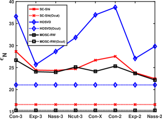
(a) $\epsilon_{N}$ on YouTube

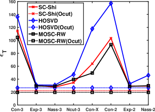
(b) $\epsilon_{T}$ on YouTube

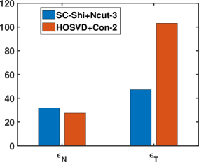
(c) Non-monotonic relationship on YouTube

Figure 2: Clustering performance of SC-Shi, HOSVD, and MOSC-RW($\lambda=0.5$) in terms of mis-clustered nodes ($\epsilon_{N}$) and triangles ($\epsilon_{T}$) for eight cut criteria: Conduct₃(Con-3), Exp₃, Nassoc₃(Nass-3), Ncut₃, Conduct-X(Con-X), Conduct₂(Con-2), Exp₂, Nassoc₂(Nass-2). Their lower bounds are provided by the optimal cut (the horizontal dotted lines). We can observe the best criterion (Nass₃) for $\epsilon_{T}$ for all algorithms, non-monotonic relationship between HOSVD+Ncut₃ vs. SC-Shi+Con₂ on $\epsilon_{N}$ and $\epsilon_{T}$ as shown in 22(c), and the superiority of Ocut for MOSC-RW.

We study three versions for each MOSC:

1. MOSC ($\lambda=0.5$): MOSC with a fixed (recommended) $\lambda$ value of $0.5$;

2. MOSC (Auto-$\lambda$): MOSC with automatically determined $\lambda$;

3. MOSC (O-$\lambda$): This version of MOSC varies $\lambda$ (with step 0.1) to find the optimal $\lambda$ (O-$\lambda$) that gives the smallest clustering error (using the ground truth). It provides a reference of the best possible results, showing the potential of the MOSC model.

Additionally, for MOSC-RW, we study simplified TSC (STSC) when $\lambda=0$.

Evaluation metrics. We use the proposed structure-aware metrics, mis-clustered edges ($\epsilon_{E}$) and triangles ($\epsilon_{T}$). We also use two popular metrics, mis-clustered nodes (Eq. (22)) and normalised mutual information (NMI) [38, 4]. For the SNAP networks, we show the average results of the 500 bi-partitioning networks.

To define NMI, we need the Shannon entropy for $\mathbb{S}$ that can be defined as $H(\mathbb{S})=-\sum^{k}_{c=1}(n_{S_{c}}/n)\log(n_{S_{c}}/n)$, where $n_{S_{c}}$ is the number of vertices in community $S_{c}$. The mutual information between $\mathbb{S}$ and $\mathbb{S}^{*}$ can be expressed as

$$I(\mathbb{S},\mathbb{S}^{*})=\sum_{c=1}^{k}\sum_{d=1}^{k}\frac{n_{S_{c}S^{*}_{d}}}{n}\log(\frac{n_{S_{c}S^{*}_{d}}/n}{(n_{S_{c}}/n)\times(n_{S^{*}_{d}}/n)}),$$ (25)

where $n_{S_{c}S^{*}_{d}}$ is the number of vertices shared by communities $S_{c}$ and $S_{d}^{*}$. The NMI between two partitions $\mathbb{S}$ and $\mathbb{S}^{*}$ is defined as

$$\text{NMI}(\mathbb{S},\mathbb{S}^{*})=\frac{2I(\mathbb{S},\mathbb{S}^{*})}{H(\mathbb{S})+H(\mathbb{S}^{*})}.$$ (26)

If $\mathbb{S}$ and $\mathbb{S}^{*}$ are identical, $\text{NMI}(\mathbb{S},\mathbb{S}^{*})$ = 1. If $\mathbb{S}$ and $\mathbb{S}^{*}$ are independent, $\text{NMI}(\mathbb{S},\mathbb{S}^{*})$ = 0.

Reproducibility. We implemented compared algorithms using Matlab code released by the authors of MSC, HOSVD, HOSPLOC, and TSC via multilinear PageRank. We followed guidance from the original papers to set their hyperparameters. All experiments were performed on a Linux machine with one 2.4GHz Intel Core and 16G memory. We have released the Matlab code for MOSC.

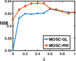
(a) NMI on DBLP

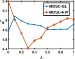
(b) $\epsilon_{N}$ on DBLP

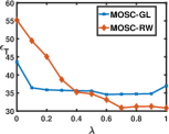
(c) $\epsilon_{T}$ on DBLP

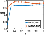
(d) NMI on Orkut

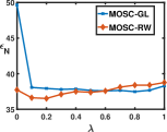
(e) $\epsilon_{N}$ on Orkut

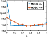
(f) $\epsilon_{T}$ on Orkut

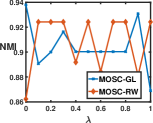
(g) NMI on Football

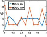
(h) $\epsilon_{N}$ on Football

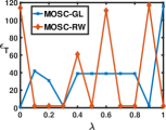
(i) $\epsilon_{T}$ on Football

Figure 3: Sensitivity analysis of $\lambda$ on DBLP, Orkut and Football w.r.t NMI, $\epsilon_{N}$ and $\epsilon_{T}$.

IV-B Effect of Cut Criteria

Firstly, we study the effect of cut criteria on clustering performance. Note that Nassoc₂ (${\xi_{2}}$) and Ncut₂ (${\eta_{2}}$) are equivalent [30], but Nassoc₃ (${\xi_{3}}$) and Ncut₃ (${\eta_{3}}$) are not (see Appendix). Thus, we have seven different cut criteria from Table I and the proposed mixed-order conductance ($\phi_{X}$) defined in Eq. (15). We study their effect on all algorithms while only reporting representative results from SC-Shi, HOSVD and MOSC-RW ($\lambda=0.5$) on YouTube.

Fig. 2 shows the results for the two metrics $\epsilon_{N}$ and $\epsilon_{T}$, together with the Ocut values (the best possible cut, knowing the ground truth). We have the following observations:

1. Cut criteria have significant impact on the performance. Among all criteria, Nassoc₃ consistently gives the smallest $\epsilon_{T}$ for all algorithms on YouTube.

2. The metric $\epsilon_{N}$ does not have a monotonic relationship with $\epsilon_{T}$. We show an example on YouTube in Fig. 22(c) with respect to $\epsilon_{N}$ and $\epsilon_{T}$. As we can see, HOSVD+Ncut₃ vs. SC-Shi+Conduct₂ on $\epsilon_{N}$ has opposite relationship on $\epsilon_{T}$.

3. The Ocut of MOSC-RW outperforms those of SC-Shi and HOSVD on both metrics $\epsilon_{N}$ and $\epsilon_{E}$ in YouTube, indicating the greater potential of MOSC-RW (even with a fixed $\lambda$). Regarding Ocut of MOSC-GL, we will present the results in Sec. IV-D.

4. Nassoc₃ and Ncut₃ are indeed not equivalent, as to be proven in Appendix.

TABLE III: Performance of clustering algorithms with the best cut criteria. The best is in bold and the second best is underlined, not considering MOSC(O-$\lambda$). A larger NMI indicates a better result, while a smaller $\epsilon_{N}$/$\epsilon_{E}$/$\epsilon_{T}$ indicates a better result. The corresponding best cut criteria are shown in parenthesis: Conduct₃ ($\phi_{3}$), Nassoc₃ (${\xi}_{3}$), Expan₃ ($\alpha_{3}$), Ncut₃ (${\eta_{3}}$), Con-X ($\phi_{X}$), Conduct₂ ($\phi_{2}$), Expan₂ ($\alpha_{2}$), Nassoc₂ (${\xi}_{2}$), $k$-means(KM).

		Second order		Third order					MOSC-RW			MOSC-GL
Method		SC-Shi	SC-Ng	HOSVD	MSC	TSC	HOSPLOC	STSC	$\lambda$ = 0.5	Auto-$\lambda$	O-$\lambda$	$\lambda$ = 0.5	Auto-$\lambda$	O-$\lambda$
DBLP	NMI	0.650 ($\phi_{2}$)	0.656 (KM)	0.550 ($\xi_{2}$)	0.620 ($\phi_{2}$)	0.648 ($\phi_{2}$)	0.286 ($\phi_{3}$)	0.628 ($\phi_{2}$)	0.654 ($\phi_{2}$)	0.646 ($\phi_{2}$)	0.795 (KM)	0.648 ($\phi_{2}$)	0.645 ($\phi_{2}$)	0.711 (KM)
	$\epsilon_{N}$	4.13 ($\eta_{3}$)	4.56 ($\eta_{3}$)	5.40 ($\xi_{3}$)	4.65 (KM)	4.30 (KM)	17.28 ($\phi_{3}$)	4.24 (KM)	4.43 ($\eta_{3}$)	4.76 ($\phi_{X}$)	1.76 (KM)	4.82 (KM)	4.87 ($\phi_{2}$)	2.76 (KM)
	$\epsilon_{E}$	13.36 ($\xi_{3}$)	14.58 ($\xi_{3}$)	17.99 ($\xi_{3}$)	15.98 ($\xi_{3}$)	18.72 ($\xi_{3}$)	70.49 ($\phi_{3}$)	18.72 ($\xi_{3}$)	14.27 ($\xi_{3}$)	15.68 ($\xi_{3}$)	6.67 (KM)	15.87 ($\xi_{3}$)	16.67 ($\xi_{2}$)	9.56 (KM)
	$\epsilon_{T}$	24.81 ($\xi_{3}$)	26.84 ($\xi_{3}$)	32.18 ($\xi_{3}$)	29.57 ($\xi_{2}$)	37.93 ($\xi_{3}$)	236.65 ($\phi_{3}$)	45.46 ($\xi_{3}$)	29.23 ($\xi_{3}$)	28.46 ($\xi_{3}$)	11.85 (KM)	30.30 ($\xi_{3}$)	32.01 ($\eta_{3}$)	20.37 (KM)
YouTube	NMI	0.248 ($\eta_{3}$)	0.270 ($\eta_{3}$)	0.124 ($\xi_{2}$)	0.184 (KM)	-	-	0.150 ($\xi_{2}$)	0.284 (KM)	0.260 ($\phi_{2}$)	0.386 (KM)	0.275 (KM)	0.263 ($\phi_{2}$)	0.335 ($\eta_{3}$)
	$\epsilon_{N}$	22.48 ($\xi_{2}$)	23.31 ($\xi_{2}$)	25.69 ($\alpha_{3}$)	24.41 ($\alpha_{3}$)	-	-	23.83 ($\xi_{3}$)	22.18 ($\xi_{2}$)	23.46 ($\xi_{2}$)	16.38 (KM)	23.44 ($\xi_{2}$)	23.83 ($\xi_{2}$)	18.45 ($\xi_{3}$)
	$\epsilon_{E}$	44.42 ($\xi_{2}$)	46.46 ($\alpha_{2}$)	50.61 ($\alpha_{3}$)	47.18 ($\alpha_{2}$)	-	-	63.12 ($\xi_{3}$)	44.28 ($\xi_{2}$)	46.74 ($\alpha_{2}$)	36.08 ($\xi_{2}$)	52.58 ($\xi_{2}$)	47.96 ($\alpha_{2}$)	37.96 (KM)
	$\epsilon_{T}$	27.70 ($\xi_{3}$)	29.49 ($\alpha_{2}$)	30.78 ($\xi_{3}$)	29.1 ($\alpha_{2}$)	-	-	59.78 ($\xi_{3}$)	28.90 ($\alpha_{2}$)	29.29 ($\alpha_{2}$)	22.15 ($\xi_{3}$)	38.63 ($\xi_{3}$)	29.46 ($\alpha_{2}$)	22.95 (KM)
Orkut	NMI	0.397 ($\eta_{3}$)	0.397 ($\eta_{3}$)	0.3618 ($\xi_{2}$)	0.390 ($\xi_{2}$)	-	-	0.387 ($\xi_{2}$)	0.410 (KM)	0.393 ($\xi_{2}$)	0.472 (KM)	0.397 (KM)	0.394 ($\xi_{2}$)	0.423 ($\eta_{3}$)
	$\epsilon_{N}$	37.13 ($\xi_{2}$)	37.09 ($\xi_{2}$)	40.43 ($\xi_{2}$)	38.49 ($\eta_{3}$)	-	-	37.60 ($\xi_{2}$)	36.05 (KM)	37.02 ($\xi_{2}$)	28.24 (KM)	36.72 ($\xi_{2}$)	36.93 ($\xi_{2}$)	32.98 (KM)
	$\epsilon_{E}$	574.6 ($\xi_{3}$)	574.6 ($\xi_{3}$)	624.7 ($\xi_{3}$)	582.3 ($\xi_{3}$)	-	-	569.2 ($\xi_{3}$)	521.6 ($\alpha_{2}$)	571.8 ($\xi_{3}$)	410.3 ($\alpha_{3}$)	550.4 ($\xi_{3}$)	574.9 ($\xi_{3}$)	497.7 ($\xi_{3}$)
	$\epsilon_{T}$	4557 ($\xi_{3}$)	4557 ($\xi_{3}$)	4937 ($\xi_{3}$)	4575 ($\xi_{3}$)	-	-	5104 ($\xi_{3}$)	3949 ($\alpha_{3}$)	4541 ($\xi_{3}$)	2944 ($\alpha_{3}$)	4405 ($\xi_{3}$)	4614 ($\xi_{3}$)	3816 ($\xi_{3}$)
LJ	NMI	0.226 ($\xi_{3}$)	0.224 ($\xi_{3}$)	0.218 ($\eta_{3}$)	0.224 ($\xi_{3}$)	0.214 ($\xi_{2}$)	-	0.201 ($\eta_{3}$)	0.229 ($\xi_{3}$)	0.221 ($\xi_{3}$)	0.271 (KM)	0.208 ($\xi_{3}$)	0.212 ($\xi_{3}$)	0.238 ($\xi_{3}$)
	$\epsilon_{N}$	5.58 ($\xi_{3}$)	5.63 ($\xi_{3}$)	5.79 ($\xi_{3}$)	5.74 ($\xi_{3}$)	5.52 ($\xi_{3}$)	-	5.15 ($\xi_{3}$)	5.49 ($\xi_{3}$)	5.66 ($\xi_{3}$)	4.43 ($\xi_{3}$)	5.76 ($\xi_{3}$)	5.64 ($\xi_{3}$)	4.98 ($\xi_{3}$)
	$\epsilon_{E}$	49.83 ($\xi_{3}$)	50.01 ($\xi_{3}$)	55.09 ($\xi_{3}$)	52.54 ($\xi_{3}$)	58.19 ($\xi_{3}$)	-	57.06 ($\xi_{3}$)	47.88 ($\xi_{3}$)	51.01 ($\xi_{3}$)	41.63 ($\xi_{3}$)	58.64 ($\xi_{3}$)	54.17 ($\xi_{3}$)	46.51 ($\xi_{3}$)
	$\epsilon_{T}$	546.1 ($\xi_{3}$)	547.6 ($\xi_{3}$)	600.6 ($\xi_{3}$)	574.5 ($\xi_{3}$)	737.7 ($\xi_{3}$)	-	773.0 ($\xi_{3}$)	530.6 ($\xi_{3}$)	556.4 ($\xi_{3}$)	460.2 ($\xi_{3}$)	730.3 ($\xi_{3}$)	617.8 ($\xi_{3}$)	539.2 ($\xi_{3}$)

TABLE IV: Clustering performance of algorithms with the best cut criteria. The best is in bold and the second best is underlined, not considering MOSC(O-$\lambda$), which makes use of the ground truth. A larger NMI indicates a better result, while a smaller $\epsilon_{N}$/$\epsilon_{E}$/$\epsilon_{T}$ indicates a better result. Note that there are ties.

		Second order		Third order				MOSC-RW			MOSC-GL
Method		SC-Shi	SC-Ng	HOSVD	MSC	TSC	STSC	$\lambda$ = 0.5	Auto-$\lambda$	O-$\lambda$	$\lambda$ = 0.5	Auto-$\lambda$	O-$\lambda$
Zachary	NMI	0.837	0.837	0.069	0.732	0.677	0.325	0.837	0.837	0.837	0.837	0.837	0.837
	$\epsilon_{N}$	1	1	14	2	2	8	1	1	1	1	1	1
	$\epsilon_{E}$	2	2	34	3	3	24	2	2	2	2	2	2
	$\epsilon_{T}$	1	1	16	1	1	14	1	1	1	1	1	1
Football	NMI	0.883	0.904	0.896	0.924	0.866	0.862	0.924	0.924	0.924	0.9	0.931	0.938
	$\epsilon_{N}$	23	15	16	10	26	26	10	10	10	15	9	7
	$\epsilon_{E}$	63	37	36	7	70	72	7	7	7	36	7	3
	$\epsilon_{T}$	99	50	39	2	110	114	2	2	2	39	2	1
Polbooks	NMI	0.575	0.542	0.092	0.542	0.180	0.103	0.575	0.575	0.581	0.563	0.589	0.589
	$\epsilon_{N}$	17	18	56	18	55	51	17	17	16	17	17	17
	$\epsilon_{E}$	27	33	185	34	281	172	27	27	27	28	21	21
	$\epsilon_{T}$	7	10	234	8	384	227	7	7	7	7	1	1
Dolphin	NMI	0.889	0.889	0.081	0.536	0.582	0.631	0.889	0.889	0.889	0.889	1	1
	$\epsilon_{N}$	1	1	19	7	6	5	1	1	1	1	0	0
	$\epsilon_{E}$	1	1	43	10	8	6	1	1	1	1	0	0
	$\epsilon_{T}$	0	0	29	0	1	0	0	0	0	0	0	0
PBlogs	NMI	0.007	0.007	0.014	0.023	-	0.430	0.012	0.458	0.557	0.098	0.016	0.098
	$\epsilon_{N}$	671	732	677	614	-	204	659	230	151	478	647	478
	$\epsilon_{E}$	7302	7302	7307	7260	-	362	7302	184	155	7302	7301	7301
	$\epsilon_{T}$	36401	36402	36400	36400	-	631	36401.5	456	410	36402	36400	36400

IV-C Effect of $\lambda$

The mixing parameter $\lambda$ is the only hyperparamter in MOSC. To gain insight of MOSC, we conduct sensitivity analysis on $\lambda$ as shown in Fig. 3 w.r.t. NMI, $\epsilon_{N}$ and $\epsilon_{T}$. We have the following observations:

1. The choice of $\lambda$ can significantly affect the performance in all datasets. This was the motivation of developing schemes to automatically determine the best $\lambda$.

2. Overall, MOSC-RW is more sensitive to $\lambda$ than MOSC-GL. We will explain the reason at the end of Sec. IV-D.

IV-D Performance Comparison

We study the results of all algorithms in combination of all eight criteria and $k$-means (KM). Figure 2 shows that cut criteria can affect the performance of all algorithms. Therefore, for fair comparison, we report the clustering results conducted by the best criteria for each algorithm. The top two results are in bold (best) or underlined (second best), without considering the O-$\lambda$ version since it uses the ground truth. O-$\lambda$ is only used for gaining insights rather than direct performance comparison with existing methods.

Results on SNAP Networks. We show the performance of all clustering algorithms with the best cut criteria in terms of NMI, $\epsilon_{N}$, $\epsilon_{E}$, and $\epsilon_{T}$ on SNAP networks in Table III. In addition, we report the best cut criteria. The results for some settings of TSC and HOSPLOC are not available either due to long running time (not finished within 40 hours) or out of memory. In particular, the multilinear PageRank algorithm in TSC is very expensive.

We have four observations:

1. MOSC-RW ($\lambda=0.5$) achieves the best in 10 out of 16 settings;

2. MOSC-RW outperforms MOSC-GL, although MOSC-GL achieves top two results in 4 settings.

3. Both MOSC-RW($\lambda=0.5$) and MOSC-GL($\lambda=0.5$) have better results than MOSC-RW(Auto-$\lambda$) and MOSC-GL(Auto-$\lambda$). This demonstrates that a fixed mixing parameter is effective, but it also shows the automatic schemes are not effective in these settings.

4. MOSC-RW(O-$\lambda$) has the highest NMI and lowest $\epsilon_{N}$, $\epsilon_{E}$, and $\epsilon_{T}$ in all 16 settings. This indicates potential future improvement by designing a better strategy to determine $\lambda$.

5. Third-order cut criteria outperform second-order cut criteria on the whole. In all 16 settings, third-order cut criteria achieve the best performance in 8 settings among which Nassoc₃ is the best in 6 settings. Second-order cut criteria achieves the best in 5 settings and $k$-means for 3 settings.

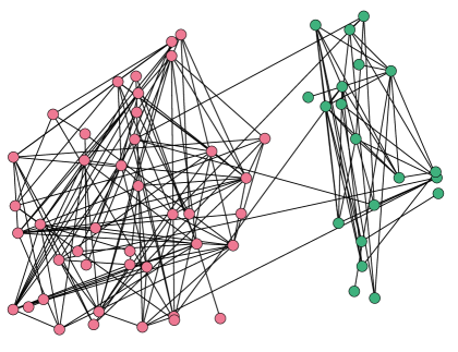
(a) Dolphin

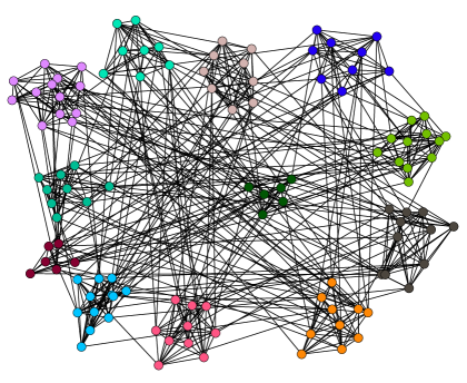
(b) Football (12 clusters)

Figure 4: Clusters in Dolphin and Football networks discovered by MOSC-GL (Auto-$\lambda$).

Results on Full Networks. We show the performance of all clustering algorithms with the best cut criteria for five full networks in terms of NMI, $\epsilon_{N}$, $\epsilon_{E}$, and $\epsilon_{T}$ in Table IV, except HOSPLOC, for which we were not able to obtain comparable results. We have three observations:

1. MOSC-GL (Auto-$\lambda$) achieves the best performance in 16 out of 20 settings, demonstrating that automatic determination of $\lambda$ is effective in these settings. Specifically, for Dolphin, MOSC-GL (Auto-$\lambda$) produces perfect results in all metrics. We visualise the obtained clusters in Dolphin as shown in Fig. 44(a). For networks with multiple clusters (Polbooks, Football), MOSC-GL (Auto-$\lambda$) is also superior to others. We visualise Football with the 12 clusters in Fig. 44(b).

2. MOSC-GL (Auto-$\lambda$) outperforms MOSC-RW (Auto-$\lambda$), although MOSC-RW (Auto-$\lambda$) achieves the best results in 10 settings, which is still better than all existing SC algorithms (Note that there are ties).

3. MOSC-GL has better model quality than MOSC-RW based on Ocut. MOSC-GL (O-$\lambda$) achieves the highest NMI and lowest $\epsilon_{N}$, $\epsilon_{E}$, and $\epsilon_{T}$ in 15 out of 20 settings while MOSC-RW (O-$\lambda$) achieves the best in 10 settings (again there are ties).

From the above results, we see that MOSC-GL and MOSC-RW have different performance on networks with different triangle densities. MOSC-RW tends to be better for networks with high triangle densities while MOSC-GL tends to be better for networks with low triangle densities. For MOSC-GL, $\mathbf{W}_{T}$ can dominate $\mathbf{W}_{X}$ in $\mathbf{W}_{X}=(1-\lambda)\mathbf{W}_{T}+\lambda\mathbf{W}$, especially for dense networks. Each entry of $\mathbf{W}_{T}$ denotes the number of triangles containing the corresponding edge while $\mathbf{W}$ is a binary matrix. Therefore, for most non-zero pairs $(i,j$), $\mathbf{W}_{T}(i,j)$ is much larger than $\mathbf{W}(i,j)$ especially for dense networks. This can be the reason that MOSC-GL is less sensitive to tuning $\lambda$, or finding the appropriate $\lambda$ is more difficult. That is, $\mathbf{W}_{X}$ tends to encode much less edge information. In contrast, MOSC-RW does not have such issue since $\mathbf{A}$ and $\mathbf{P}$ are normalised and thus they are in similar scales before linear combination. Therefore, MOSC-RW has a better performance than MOSC-GL in SNAP networks and the dense full graph PBlogs.

IV-E Computational Time

Figure 5 compares the computational time of different methods on YouTube, LJ, PBlogs and Football, using $k$-means to obtain the final clusters to avoid the effect of cut criteria. We have the following observations:

1. Both HOSVD and MOSC-RW involve tensor construction and operations so they are both more time consuming, in particular on dense networks such as LJ and PBlogs, where HOSVD is the slowest and MOSC-RW is the second slowest. The reason is that HOSVD uses more a complicated dimension reduction method than MOSC-RW.

2. MOSC-GL is more efficient than MOSC-RW in all cases and has similar efficiency as conventional SC methods on the whole.

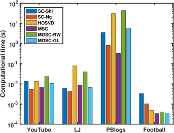
Figure 5: Computational time (in log scale) on YouTube, LJ, PBlogs and Football.

V Conclusion

This paper proposed two mixed-order spectral clustering (MOSC) methods, MOSC-GL and MOSC-RW, which model both second-order and third-order structures for network clustering. MOSC-GL combines edge and triangle adjacency matrices with theoretical performance guarantee. MOSC-RW combines first-order and second-order random walks with a probabilistic interpretation. We designed a scheme to automatically determine the mixing parameter and new structure-aware error metrics for structure evaluation. We also defined an optimal cut to study the lower error bound for exploring potentials of MOSC. Experiments on 2,005 networks showed that MOSC algorithms outperform existing SC methods in most cases and the proposed mixed-order approach produces more superior clustering of networks.

Appendix A Proof of the Relationship between Ncut₃ and Nassoc₃

Shi and Malik [12] showed that second-order normalised cut (Ncut₂) and association (Nassoc₂) are equivalent by the following equation:

$$Ncut_{2}(S;G)=2-Nassoc_{2}(S;G),$$ (27)

which indicates that the minimisation of Ncut₂ is equivalent to maximisation of Nassoc₂. It inspires us to think about a question: does third-order normalised cut (Ncut₃) [31] and association (Nassoc₃) [23] have the similar equivalence?

Based on the definition of $cut_{3}(S)$, we have the following equation [25] (omitting $G$):

$$cut_{3}(\emph{S},\bar{\emph{S}}) = \frac{1}{3}(((vol_{3}(\emph{S})-assoc_{3}(\emph{S}))$$ (28)

$$+(vol_{3}(\bar{\emph{S}})-assoc_{3}(\bar{\emph{S}}))).$$

Ncut${}_{3}(S)$ [31] is defined as follows:

$$Ncut_{3}(\emph{S}) =cut_{3}({\emph{S},\bar{\emph{S}}})(\frac{1}{{vol_{3}({\emph{S}})}}+\frac{1}{vol_{3}({\bar{\emph{S}})}}).$$ (29)

This gives that:

$$Ncut_{3}(\emph{S}) =\frac{(vol_{3}(\emph{S})-assoc_{3}(\emph{S}))+(vol_{3}(\bar{\emph{S}})-assoc_{3}(\bar{\emph{S}}))}{{3vol_{3}({\emph{S}})}}$$ (30)

$$+\frac{(vol_{3}(\emph{S})-assoc_{3}(\emph{S}))+(vol_{3}(\bar{\emph{S}})-assoc_{3}(\bar{\emph{S}}))}{{3vol_{3}({\bar{\emph{S}}})}}$$

$$=\frac{2}{3}-\frac{1}{3}(\frac{assoc_{3}(\emph{S})}{vol_{3}(\emph{S})}+\frac{assoc_{3}(\bar{\emph{S}})}{vol_{3}(\bar{\emph{S}})})$$

$$+\frac{1}{3}(\frac{{vol_{3}({\bar{\emph{S}}})}-assoc_{3}(\bar{{\emph{S}})}}{vol_{3}({\emph{S}})}+\frac{{vol_{3}({\emph{S}})}-assoc_{3}({\emph{S})}}{vol_{3}({\bar{\emph{S}}})})$$

The definition of $Nassoc_{3}(S)$ [23] is given as:

$$Nassoc_{3}(S)=\frac{assoc_{3}(\emph{S})}{vol_{3}(\emph{S})}+\frac{assoc_{3}(\bar{\emph{S}})}{vol_{3}(\bar{\emph{S}})}$$ (31)

The above equations indicate:

$$Ncut_{3}(\emph{S}) =\frac{2}{3}-\frac{1}{3}Nassoc_{3}(S)$$ (32)

$$+\frac{1}{3}(\frac{{vol_{3}({\bar{\emph{S}}})}-assoc_{3}({\bar{\emph{S}})}}{vol_{3}({\emph{S}})}+\frac{{vol_{3}({\emph{S}})}-assoc_{3}({\emph{S})}}{vol_{3}({\bar{\emph{S}}})}).$$

From Eq. (32), we can see that the third term in is not a constant. Therefore, minimisation of Ncut₃ is not equivalent to maximisation of Nassoc₃.

References

- [1] A. R. Benson, D. F. Gleich, and J. Leskovec, “Higher-order organization of complex networks,” Science, vol. 353, no. 6295, pp. 163–166, 2016.
- [2] C. Liu, J. Liu, and Z. Jiang, “A multiobjective evolutionary algorithm based on similarity for community detection from signed social networks,” IEEE Trans. Cybern., vol. 44, no. 12, pp. 2274–2287, 2014.
- [3] L. Yang, X. Cao, D. Jin, X. Wang, and D. Meng, “A unified semi-supervised community detection framework using latent space graph regularization,” IEEE Trans. Cybern., vol. 45, no. 11, pp. 2585–2598, 2015.
- [4] H. Chang, Z. Feng, and Z. Ren, “Community detection using dual-representation chemical reaction optimization,” IEEE Trans. Cybern., vol. 47, no. 12, pp. 4328–4341, 2017.
- [5] L. Zhang, H. Pan, Y. Su, X. Zhang, and Y. Niu, “A mixed representation-based multiobjective evolutionary algorithm for overlapping community detection,” IEEE Trans. Cybern., vol. 47, no. 9, pp. 2703–2716, 2017.
- [6] Z. Li, J. Liu, and K. Wu, “A multiobjective evolutionary algorithm based on structural and attribute similarities for community detection in attributed networks,” IEEE Trans. Cybern., vol. 48, no. 7, pp. 1963–1976, 2018.
- [7] A. Clauset, M. E. Newman, and C. Moore, “Finding community structure in very large networks,” Physical Review E, vol. 70, no. 6, p. 066111, 2004.
- [8] S. E. Schaeffer, “Graph clustering,” Computer science review, vol. 1, no. 1, pp. 27–64, 2007.
- [9] M. A. Porter, J.-P. Onnela, and P. J. Mucha, “Communities in networks,” Notices of the AMS, vol. 56, no. 9, pp. 1082–1097, 2009.
- [10] S. Fortunato, “Community detection in graphs,” Physics Reports, vol. 486, no. 3-5, pp. 75–174, 2010.
- [11] M. E. Newman, “Communities, modules and large-scale structure in networks.” Nature Physics, vol. 8, no. 1, 2012.
- [12] M. Meila and J. Shi, “Learning segmentation by random walks,” in Advances in Neural Information Processing Systems, 2001, pp. 873–879.
- [13] A. Y. Ng, M. I. Jordan, and Y. Weiss, “On spectral clustering: Analysis and an algorithm,” in Advances in Neural Information Processing Systems, 2002, pp. 849–856.
- [14] A. R. Benson, D. F. Gleich, and J. Leskovec, “Tensor spectral clustering for partitioning higher-order network structures,” in Proceedings of the 2015 SIAM International Conference on Data Mining. SIAM, 2015, pp. 118–126.
- [15] D. Zhou, S. Zhang, M. Y. Yildirim, S. Alcorn, H. Tong, H. Davulcu, and J. He, “A local algorithm for structure-preserving graph cut,” in Proceedings of the 23rd ACM SIGKDD International Conference on Knowledge Discovery and Data Mining. ACM, 2017, pp. 655–664.
- [16] R. Milo, S. Shen-Orr, S. Itzkovitz, N. Kashtan, D. Chklovskii, and U. Alon, “Network motifs: simple building blocks of complex networks,” Science, vol. 298, no. 5594, pp. 824–827, 2002.
- [17] O. Sporns and R. Kötter, “Motifs in brain networks,” PLoS Biology, vol. 2, no. 11, p. e369, 2004.
- [18] M. S. Granovetter, “The strength of weak ties,” in Social Networks. Elsevier, 1977, pp. 347–367.
- [19] G. Kossinets and D. J. Watts, “Empirical analysis of an evolving social network,” science, vol. 311, no. 5757, pp. 88–90, 2006.
- [20] B. Serrour, A. Arenas, and S. Gómez, “Detecting communities of triangles in complex networks using spectral optimization,” Computer Communications, vol. 34, no. 5, pp. 629–634, 2011.
- [21] D. Ghoshdastidar and A. Dukkipati, “Spectral clustering using multilinear svd: Analysis, approximations and applications.” in AAAI, 2015, pp. 2610–2616.
- [22] ——, “Consistency of spectral partitioning of uniform hypergraphs under planted partition model,” in Advances in Neural Information Processing Systems, 2014, pp. 397–405.
- [23] ——, “Uniform hypergraph partitioning: Provable tensor methods and sampling techniques,” Journal of Machine Learning Research, vol. 18, no. 50, pp. 1–41, 2017.
- [24] T. Wu, A. R. Benson, and D. F. Gleich, “General tensor spectral co-clustering for higher-order data,” in Advances in Neural Information Processing Systems, 2016, pp. 2559–2567.
- [25] C. E. Tsourakakis, J. Pachocki, and M. Mitzenmacher, “Scalable motif-aware graph clustering,” in Proceedings of the 26th International Conference on World Wide Web. International World Wide Web Conferences Steering Committee, 2017, pp. 1451–1460.
- [26] H. Yin, A. R. Benson, J. Leskovec, and D. F. Gleich, “Local higher-order graph clustering,” in Proceedings of the 23rd ACM SIGKDD International Conference on Knowledge Discovery and Data Mining. ACM, 2017, pp. 555–564.
- [27] U. Von Luxburg, “A tutorial on spectral clustering,” Statistics and Computing, vol. 17, no. 4, pp. 395–416, 2007.
- [28] J. Xu, T. L. Wickramarathne, and N. V. Chawla, “Representing higher-order dependencies in networks,” Science Advances, vol. 2, no. 5, p. e1600028, 2016.
- [29] F. D. Malliaros and M. Vazirgiannis, “Clustering and community detection in directed networks: A survey,” Physics Reports, vol. 533, no. 4, pp. 95–142, 2013.
- [30] J. Shi and J. Malik, “Normalized cuts and image segmentation,” IEEE Trans. on Pattern Analysis and Machine Intelligence, vol. 22, no. 8, pp. 888–905, 2000.
- [31] P. Li and O. Milenkovic, “Inhomogoenous hypergraph clustering with applications,” in Advances in Neural Information Processing Systems, 2017, pp. 2305–2315.
- [32] G. W. Flake, R. E. Tarjan, and K. Tsioutsiouliklis, “Graph clustering and minimum cut trees,” Internet Mathematics, vol. 1, no. 4, pp. 385–408, 2004.
- [33] M. Fiedler, “Algebraic connectivity of graphs,” Czechoslovak Mathematical Journal, vol. 23, no. 2, pp. 298–305, 1973.
- [34] J. R. Lee, S. O. Gharan, and L. Trevisan, “Multiway spectral partitioning and higher-order cheeger inequalities,” Journal of the ACM (JACM), vol. 61, no. 6, p. 37, 2014.
- [35] J. Leskovec, K. J. Lang, and M. Mahoney, “Empirical comparison of algorithms for network community detection,” in Proceedings of the 19th International Conference on World Wide Web. ACM, 2010, pp. 631–640.
- [36] T. Chakraborty, A. Dalmia, A. Mukherjee, and N. Ganguly, “Metrics for community analysis: A survey,” ACM Computing Surveys (CSUR), vol. 50, no. 4, p. 54, 2017.
- [37] J. Yang and J. Leskovec, “Defining and evaluating network communities based on ground-truth,” Knowledge and Information Systems, vol. 42, no. 1, pp. 181–213, 2015.
- [38] L. Ana and A. K. Jain, “Robust data clustering,” in Computer Vision and Pattern Recognition, 2003. Proceedings. 2003 IEEE Computer Society Conference on, vol. 2. IEEE, 2003, pp. II–II.
- [39] W. W. Zachary, “An information flow model for conflict and fission in small groups,” Journal of Anthropological Research, vol. 33, no. 4, pp. 452–473, 1977.
- [40] D. Lusseau, “The emergent properties of a dolphin social network,” Proceedings of the Royal Society of London B: Biological Sciences, vol. 270, no. Suppl 2, pp. S186–S188, 2003.
- [41] M. E. Newman, “Modularity and community structure in networks,” Proceedings of the national academy of sciences, vol. 103, no. 23, pp. 8577–8582, 2006.
- [42] L. A. Adamic and N. Glance, “The political blogosphere and the 2004 us election: divided they blog,” in Proceedings of the 3rd international workshop on Link discovery. ACM, 2005, pp. 36–43.
- [43] D. F. Gleich, L.-H. Lim, and Y. Yu, “Multilinear pagerank,” SIAM Journal on Matrix Analysis and Applications, vol. 36, no. 4, pp. 1507–1541, 2015.