Boundary conditions for the Stokes problem and
a pressure-Poisson problem

Abstract

We consider a boundary value problem for the stationary Stokes problem and the corresponding pressure-Poisson equation. We propose a new formulation for the pressure-Poisson problem with an appropriate additional boundary condition. We establish error estimates between solutions to the Stokes problem and the pressure-Poisson problem in terms of the additional boundary condition. As boundary conditions for the Stokes problem, we use a traction boundary condition and a pressure boundary condition introduced in C. Conca et al (1994).

Key words: Stokes problem, Pressure-Poisson equation
2010 MSC: 35Q35, 35A35, 76D07

1 Introduction

Let $\Omega$ be a bounded connected open set of ${\mathbb{R}}^{3}$ with Lipschitz continuous boundary $\Gamma$. We assume that there exist two relatively open subsets $\Gamma_{1}$ and $\Gamma_{2}$ of $\Gamma$ such that

$$|\Gamma\setminus(\Gamma_{1}\cup\Gamma_{2})|=0,\quad|\Gamma_{1}|,|\Gamma_{2}|>0,\quad\Gamma_{1}\cap\Gamma_{2}=\emptyset,\quad\mathring{\overline{\Gamma_{1}}}=\Gamma_{1},\quad\mathring{\overline{\Gamma_{2}}}=\Gamma_{2},$$

where $\overline{A}$ is the closure of $A\subset\Gamma$ with respect to $\Gamma$, $\mathring{A}$ is the interior of $A$ with respect to $\Gamma$ and $|A|$ is the two dimensional Hausdorff measure.

The strong form of the Stokes problem is given as follows. Find $u^{S}:\Omega\rightarrow{\mathbb{R}}^{3}$ and $p^{S}:\Omega\rightarrow{\mathbb{R}}$ such that

$$\left\{\begin{array}[]{rcll}-\Delta u^{S}+\nabla p^{S}&=&F&\mbox{in }\Omega,\\ \operatorname{div}u^{S}&=&0&\mbox{in }\Omega,\\ u^{S}&=&0&\mbox{on }\Gamma_{1},\\ T_{\nu}(u^{S},p^{S})&=&t^{b}&\mbox{on }\Gamma_{2},\end{array}\right.$$ (5)

holds, where $t^{b}:\Gamma_{2}\rightarrow{\mathbb{R}}^{3}$, $\nu$ is the unit outward normal vector for $\Gamma$ and

$$T_{\nu}(u,p)_{i}:=\sum^{3}_{j=1}\left(\frac{\partial u_{i}}{\partial x_{j}}+\frac{\partial u_{j}}{\partial x_{i}}\right)\nu_{j}-p\nu_{i}\quad\mbox{for all }i=1,2,3.$$

The functions $u^{S}$ and $p^{S}$ are the velocity and the pressure of the flow governed by (5), respectively. We refer to [1] and [2] for the details on the Stokes problem (i.e., physical background and corresponding mathematical analysis). Taking the divergence of the first equation, we obtain

$$\operatorname{div}F=\operatorname{div}(-\Delta u^{S}+\nabla p^{S})=-\Delta(\operatorname{div}u^{S})+\Delta p^{S}=\Delta p^{S}.$$ (6)

This equation is often called the pressure-Poisson equation and is used in numerical schemes such as MAC (marker and sell), SMAC (simplified MAC) or the projection method (see, e.g., [3, 4, 5, 6, 7, 8, 9, 10]).

We need an additional boundary condition for solving the equation (6). In the real-would applications, the additional boundary condition is usually given by using experimental or plausible values. We consider the following boundary value problem for the pressure-Poisson equation: Find $u^{PP}:\Omega\rightarrow{\mathbb{R}}^{3}$ and $p^{PP}:\Omega\rightarrow{\mathbb{R}}$ satisfying

$$\left\{\begin{array}[]{rcll}-\Delta u^{PP}-\nabla(\operatorname{div}u^{PP})+\nabla p^{PP}&=&F&\mbox{in }\Omega,\\ -\Delta p^{PP}&=&-\operatorname{div}F&\mbox{in }\Omega,\\ u^{PP}&=&0&\mbox{on }\Gamma_{1},\\ {\displaystyle\frac{\partial p^{PP}}{\partial\nu}}&=&g^{b}&\mbox{on }\Gamma_{1},\\[8.0pt] T_{\nu}(u^{PP},p^{PP})&=&t^{b}&\mbox{on }\Gamma_{2},\\[8.0pt] p^{PP}&=&p^{b}&\mbox{on }\Gamma_{2},\end{array}\right.$$ (13)

where $g^{b}:\Gamma_{1}\rightarrow{\mathbb{R}}$, $p^{b}:\Gamma_{2}\rightarrow{\mathbb{R}}$ are the data for the additional boundary conditions. We call this problem the pressure-Poisson problem. The second term $-\nabla(\operatorname{div}u^{PP})$ in the first equation of (13) is necessary to treat the traction boundary condition in a weak formulation. The idea of using (6) instead of $\operatorname{div}u^{S}=0$ is useful for calculating the pressure numerically in the Navier–Stokes problem. For example, this idea is used in the MAC, SMAC and projection methods.

In this paper, we establish error estimates between solutions for (5) and (13) in terms of the additional boundary conditions. As the boundary condition for the Stokes problem, we also consider the boundary condition introduced in [11];

$$\left\{\begin{array}[]{rcll}u&=&0&\mbox{on }\Gamma_{1},\\ u\times\nu&=&0&\mbox{on }\Gamma_{2},\\ p&=&p^{b}&\mbox{on }\Gamma_{2},\end{array}\right.$$ (17)

where “$\times$” is the cross product in ${\mathbb{R}}^{3}$ (see also [12, 13, 14]). Since boundary conditions which contain a Dirichlet boundary condition for the pressure often appear in engineering problems, a comparison between (13) and the Stokes problem with (17) is important. For example, an end of pipe such as blood vessels or pipelines corresponds to the boundary $\Gamma_{2}$ (Fig. 1).

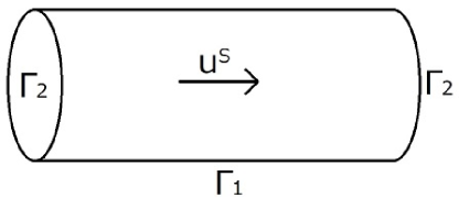
Figure 1: Image of a flow in a pipe

The organization of this paper is as follows. In Section 2 we introduce notations and symbols used in this work and the weak form of these problems. We also prove the well-posedness of the problems (5) and (13) and show several properties of them. In Section 3 we establish error estimates between solutions to the problems (5) and (13) in terms of the additional boundary conditions. Section 4 is devoted to the study of the Stokes problem with the boundary condition (17). We conclude this paper with several comments on future works in Section 5.

2 Preliminaries

2.1 Notation

We use the usual Lebesgue space ${L^{2}(\Omega)}$ and Sobolev spaces $H^{r}(\Omega)$ $=W^{r,2}(\Omega)$ for a non-negative integer $r$, together with their standard norms. For spaces of vector-valued functions, we write ${L^{2}(\Omega)}^{3}$, and so on. The space ${H^{1}_{0}(\Omega)}$ denotes the closure of $C^{\infty}_{0}(\Omega)$ in ${H^{1}(\Omega)}$. $\mathcal{D}^{\prime}(\Omega)$ denotes the space of distributions on $\Omega$. We set

$$\begin{array}[]{rcl}{H^{1}_{\Gamma_{i}}(\Omega)}&:=&\{\psi\in{H^{1}(\Omega)}\,|\,\psi=0\mbox{ on }\Gamma_{i}\}\quad(i=1,2),\\ H&:=&{\displaystyle\left\{\varphi\in{H^{1}(\Omega)}^{3}\,\middle|\,\varphi=0\mbox{ on }\Gamma_{1},\varphi\times\nu=0\mbox{ on }\Gamma_{2}\right\}.}\end{array}$$

We also use the Lebesgue space $L^{2}(\Gamma)$ and Sobolev space $H^{1/2}(\Gamma)$ defined on $\Gamma$. The norm $\|\eta\|_{H^{1/2}(\Gamma)}$ is defined by

$$\|\eta\|_{H^{1/2}(\Gamma)}:=\left(\|\eta\|^{2}_{L^{2}(\Gamma)}+\int_{\Gamma}\int_{\Gamma}\frac{|\eta(x)-\eta(y)|^{2}}{|x-y|^{3}}ds(x)ds(y)\right)^{1/2},$$

where $ds$ denotes the surface measure of $\Gamma$. For function spaces defined on $\Gamma_{i}~{}(i=1,2)$, we write $L^{2}(\Gamma_{i})$, and so on.

We further set

$$\begin{array}[]{c}{\displaystyle p_{,i}:=\frac{\partial p}{\partial x_{i}},\quad p_{,ij}:=\frac{\partial p}{\partial x_{i}\partial x_{j}},\quad D_{ij}(u):=\frac{1}{2}\left(u_{i,j}+u_{j,i}\right),}\quad{\displaystyle D(u):D(\varphi):=\sum^{3}_{l,m=1}D_{lm}(u)D_{lm}(\varphi)}\end{array}$$

for all $p:\Omega\rightarrow{\mathbb{R}},u=(u_{1},u_{2},u_{3}):\Omega\rightarrow{\mathbb{R}}^{3},\varphi=(\varphi_{1},\varphi_{2},\varphi_{3}):\Omega\rightarrow{\mathbb{R}}^{3}$ and $i,j=1,2,3$.

2.2 Preliminary results

Let $\gamma_{0}\in{\mathscr{L}}({H^{1}(\Omega)},H^{1/2}(\Gamma))$ be the standard trace operator. The trace operator $\gamma_{0}$ is surjective and satisfies $\mbox{Ker}(\gamma_{0})={H^{1}_{0}(\Omega)}$ [1, Theorem 1.5]. Let $\nu$ be the unit outward normal for $\Gamma$. Since $\nu$ is a unit vector, ${H^{1}(\Omega)}^{3}\ni u\mapsto u\cdot\nu:=(\gamma_{0}u)\cdot\nu\in H^{1/2}(\Gamma)$ is a linear continuous map. For all $u\in{H^{1}(\Omega)}^{3}$ and $p\in{H^{1}(\Omega)}$, the following Gauss divergence formula holds:

$$\int_{\Omega}u\cdot\nabla p+\int_{\Omega}(\operatorname{div}u)p=\int_{\Gamma}(u\cdot\nu)p.$$

For $i=1,2$, composition of the trace operator $\gamma_{0}$ and the restriction $H^{1/2}(\Gamma)\rightarrow H^{1/2}(\Gamma_{i})$ is denoted by $\psi\mapsto\psi|_{\Gamma_{i}}$. This map is continuous from ${H^{1}(\Omega)}$ to $H^{1/2}(\Gamma_{i})$. Since the kernel of this map is ${H^{1}_{\Gamma_{i}}(\Omega)}$, there exists a constant $c>0$ such that

$$\|\psi\|_{{H^{1}(\Omega)}/{H^{1}_{\Gamma_{i}}(\Omega)}}\leq c\|\psi|_{\Gamma_{i}}\|_{H^{1/2}(\Gamma_{i})},$$

where $\|\psi\|_{{H^{1}(\Omega)}/{H^{1}_{\Gamma_{i}}(\Omega)}}:=\inf_{q\in{H^{1}_{\Gamma_{i}}(\Omega)}}\|\psi+q\|_{H^{1}(\Omega)}$. We simply write $\psi$ instead of $\psi|_{\Gamma_{i}}$ when there is no ambiguity. We denote by $\langle\cdot,\cdot\rangle_{\Gamma_{i}}$ the duality pairing between $H^{-1/2}(\Gamma_{i}):=H^{1/2}(\Gamma_{i})^{*}$ and $H^{1/2}(\Gamma_{i})$. We remark that $\eta^{*}\in L^{2}(\Gamma_{i})$ can be identified with a element of $H^{-1/2}(\Gamma_{i})$ by

$$\langle\eta^{*},\eta\rangle_{\Gamma_{i}}:=\int_{\Gamma_{i}}\eta^{*}\eta\qquad\mbox{for all }\eta\in H^{1/2}(\Gamma_{i}).$$

For $u\in{H^{1}(\Omega)}^{3}$ and $p\in{H^{1}(\Omega)}$ satisfying $\Delta u+\nabla(\operatorname{div}u)\in{L^{2}(\Omega)}$ and $\Delta p\in{L^{2}(\Omega)}$, we set

$$\begin{array}[]{rcll}\langle D(u)\nu,\varphi\rangle_{\Gamma_{2}}&:=&{\displaystyle\int_{\Omega}\left(D(u):D(\varphi)+\frac{1}{2}(\Delta u+\nabla(\operatorname{div}u))\varphi\right)}&\mbox{for all }\varphi\in{H^{1}_{\Gamma_{1}}(\Omega)}^{3},\\[8.0pt] \hskip 5.0pt{\displaystyle\left\langle\frac{\partial p}{\partial\nu},\psi\right\rangle_{\Gamma_{1}}}&:=&{\displaystyle\int_{\Omega}\left(\nabla p\cdot\nabla\psi+(\Delta p)\psi\right)}&\mbox{for all }\psi\in{H^{1}_{\Gamma_{2}}(\Omega)}.\end{array}$$

We remark that $u\in H^{2}(\Omega)^{3}$ and $p\in H^{2}(\Omega)$ satisfy

$$\langle D(u)\nu,\varphi\rangle_{\Gamma_{2}}=\int_{\Gamma_{2}}\left(\sum^{3}_{i,j=1}D_{ij}(u)\varphi_{i}\nu_{j}\right),\quad\left\langle\frac{\partial p}{\partial\nu},\psi\right\rangle_{\Gamma_{1}}=\int_{\Gamma_{1}}\frac{\partial p}{\partial\nu}\psi$$

for all $\varphi\in{H^{1}_{\Gamma_{1}}(\Omega)}^{3}$ and $\psi\in{H^{1}_{\Gamma_{2}}(\Omega)}$. For $u\in{H^{1}(\Omega)}^{3}$ and $p\in{H^{1}(\Omega)}$ satisfying $\Delta u+\nabla(\operatorname{div}u)\in{L^{2}(\Omega)}$, we set

$$\langle T_{\nu}(u,p)\nu,\varphi\rangle_{\Gamma_{2}}:=2\langle D(u)\nu,\varphi\rangle_{\Gamma_{2}}-\int_{\Gamma_{2}}p\varphi\cdot\nu\qquad\mbox{for all }\varphi\in{H^{1}_{\Gamma_{1}}(\Omega)}^{3}.$$

We recall the following five theorems which are necessary for the existence and the uniqueness of a solution to the Stokes problem.

Theorem 2.1.

[1, Corollary 4.1] Let $(X,\|\cdot\|_{X})$ and $(Q,\|\cdot\|_{Q})$ be two real Hilbert spaces. Let $a:X\times X\rightarrow{\mathbb{R}}$ and $b:X\times Q\rightarrow{\mathbb{R}}$ be bilinear and continuous maps and let $f\in X^{*}$. If there exist two constants $\alpha>0$ and $\beta>0$ such that

$$\begin{array}[]{rcll}a(v,v)&\geq&\alpha\|v\|^{2}_{X}&\mbox{for all }v\in V,\\ {\displaystyle\sup_{v\in X\setminus\{0\}}\frac{b(v,q)}{\|v\|_{X}}}&\geq&\beta\|q\|_{Q}&\mbox{for all }q\in Q,\end{array}$$

where $V=\{v\in X~{}|~{}b(v,q)=0\mbox{ for all }q\in Q\}$, then there exists a unique solution $(u,p)\in X\times Q$ to the following problem:

$$\left\{\begin{array}[]{rcll}a(u,v)+b(v,p)&=&f(v)&\mbox{for all }v\in X,\\ b(u,q)&=&0&\mbox{for all }q\in Q.\end{array}\right.$$

Theorem 2.2.

[14, Lemma 3.4] There exists a constant $c>0$ such that

$$\sup_{\varphi\in{H^{1}_{\Gamma_{1}}(\Omega)}^{3}\setminus\{0\}}\frac{{\displaystyle\int_{\Omega}q\operatorname{div}\varphi}}{\|\varphi\|_{{H^{1}(\Omega)}^{3}}}\geq c\|q\|_{{L^{2}(\Omega)}}$$

for all $q\in{L^{2}(\Omega)}$.

The following theorem is called Korn’s second inequality.

Theorem 2.3 (Korn’s second inequality).

[15, Lemma 5.4.18] There exists a constant $c>0$ such that

$$\|D(\varphi)\|_{{L^{2}(\Omega)}^{3\times 3}}\geq c\|\varphi\|_{{H^{1}(\Omega)}^{3}}.$$

for all $\varphi\in{H^{1}_{\Gamma_{1}}(\Omega)}^{3}$.

The following embedding theorem is called Poincare’s inequality.

Theorem 2.4 (Poincare’s inequality).

[1, Lemma 3.1] There exists a constant $c>0$ such that

$$\|\nabla\varphi\|_{{L^{2}(\Omega)}^{3}}\geq c\|\varphi\|_{L^{2}(\Omega)}$$

for all $\varphi\in{H^{1}_{\Gamma_{i}}(\Omega)}~{}(i=1\mbox{ or }2)$.

The following embedding theorem plays an important role in the proof of the existence and the uniqueness of the solution to the Stokes problem with the boundary condition (17).

Theorem 2.5.

[11, Lemma 1.4] If $\Omega$ or $\Gamma$ satisfy one of the following conditions;

$$\Gamma\mbox{ is of class }C^{1,1}$$

or

$$\Omega\mbox{ is a convex polyhedron},$$

then there exists a constant $c>0$ such that

$$\|\nabla\times v\|_{{L^{2}(\Omega)}^{3}}\geq c\|v\|_{{H^{1}(\Omega)}^{3}}$$

for all $v\in H$ satisfying $\operatorname{div}v=0$.

2.3 Weak formulations of (13) and (5)

We start by defining the weak solution to (13). Throughout of this paper, we suppose the following conditions;

$$t^{b}\in H^{-1/2}(\Gamma_{2})^{3},\qquad F\in{L^{2}(\Omega)}^{3},$$ (18)

$$g^{b}\in H^{-1/2}(\Gamma_{1}),\quad p^{b}\in{H^{1}(\Omega)},\quad\operatorname{div}F\in{L^{2}(\Omega)}.$$ (19)

Lemma 2.6.

For $u\in H^{2}(\Omega)^{3},p\in H^{1}(\Omega)$ and $\varphi\in{H^{1}_{\Gamma_{1}}(\Omega)}^{3}$,

$$\int_{\Omega}(-\Delta u-\nabla(\operatorname{div}u)+\nabla p)\cdot\varphi=\frac{1}{2}\int_{\Omega}D(u):D(\varphi)-\int_{\Omega}p\operatorname{div}\varphi-\langle t,\varphi\rangle_{\Gamma_{2}}$$

holds, where $t:=T_{\nu}(u,p)$.

Proof. We compute

$$\begin{array}[]{l}\quad{\displaystyle\int_{\Omega}(-\Delta u-\nabla(\operatorname{div}u)+\nabla p)\cdot\varphi}\\[8.0pt] ={\displaystyle-\int_{\Omega}\sum^{3}_{i,j=1}(u_{i,jj}+u_{j,ij})\varphi_{i}+\int_{\Omega}\sum^{3}_{i=1}p_{,i}\varphi_{i}}\\[8.0pt] ={\displaystyle\sum^{3}_{i,j=1}\left\{\int_{\Omega}(u_{i,j}+u_{j,i})\varphi_{i,j}-\int_{\Gamma}(u_{i,j}+u_{j,i})\varphi_{i}\nu_{j}\right\}+\sum^{3}_{i=1}\left\{-\int_{\Omega}p\varphi_{i,i}+\int_{\Gamma}p\varphi_{i}\nu_{i}\right\}}\\[8.0pt] ={\displaystyle\frac{1}{2}\int_{\Omega}\sum^{3}_{i,j=1}(u_{i,j}+u_{j,i})(\varphi_{i,j}+\varphi_{j,i})-\int_{\Omega}\sum^{3}_{i=1}p\varphi_{i,i}-\int_{\Gamma}\sum^{3}_{i=1}T_{\nu}(u,p)_{i}\varphi_{i}}\\[8.0pt] ={\displaystyle\frac{1}{2}\int_{\Omega}D(u):D(\varphi)-\int_{\Omega}p\operatorname{div}\varphi-\langle t,\varphi\rangle_{\Gamma_{2}}},\end{array}$$

which completes the proof. ∎

For the second equation of (13), taking $\psi\in{H^{1}_{\Gamma_{2}}(\Omega)}$, we obtain

$$\begin{array}[]{rl}{\displaystyle-\int_{\Omega}(\operatorname{div}F)\psi}&={\displaystyle-\int_{\Omega}(\Delta p^{PP})\psi}\\[8.0pt] &={\displaystyle-\int_{\Gamma}\frac{\partial p^{PP}}{\partial\nu}\psi+\int_{\Omega}\nabla p^{PP}\cdot\nabla\psi}\\[8.0pt] &={\displaystyle-\langle g^{b},\psi\rangle_{\Gamma_{1}}+\int_{\Omega}\nabla p^{PP}\cdot\nabla\psi.}\end{array}$$

Therefore, the weak form of (13) becomes as follows. Find $u^{PP}\in{H^{1}_{\Gamma_{1}}(\Omega)}^{3}$ and $p^{PP}\in{H^{1}(\Omega)}$ such that

$$\left\{\begin{array}[]{rcll}{\displaystyle\frac{1}{2}\int_{\Omega}D(u^{PP}):D(\varphi)-\int_{\Omega}p^{PP}\operatorname{div}\varphi}&=&{\displaystyle\int_{\Omega}F\cdot\varphi-\langle t^{b},\varphi\rangle_{\Gamma_{2}}}&\mbox{for all }\varphi\in{H^{1}_{\Gamma_{1}}(\Omega)}^{3},\\[8.0pt] {\displaystyle\int_{\Omega}\nabla p^{PP}\cdot\nabla\psi}&=&{\displaystyle-\int_{\Omega}(\operatorname{div}F)\psi+\langle g^{b},\psi\rangle_{\Gamma_{1}}}&\mbox{for all }\psi\in{H^{1}_{\Gamma_{2}}(\Omega)},\\[8.0pt] p^{PP}&=&p^{b}\hskip 95.0pt\mbox{on }\Gamma_{2}.\end{array}\right.$$ (23)

Remark 2.7.

If $(u^{PP},p^{PP})\in{H^{1}_{\Gamma_{1}}(\Omega)}^{3}\times{H^{1}(\Omega)}$ satisfies $u^{PP}\in H^{2}(\Omega)^{3},p^{PP}\in H^{1}(\Omega)$ and (23), then we have

$$\left\{\begin{array}[]{rcll}{\displaystyle\int_{\Omega}(-\Delta u^{PP}-\nabla(\operatorname{div}u^{PP})+\nabla p^{PP}-F)\cdot\varphi}&=&{\displaystyle\langle T_{\nu}(u^{PP},p^{PP})-t^{b},\varphi\rangle_{\Gamma_{2}}}&\mbox{for all }\varphi\in{H^{1}_{\Gamma_{1}}(\Omega)}^{3},\\[8.0pt] {\displaystyle\int_{\Omega}(-\Delta p^{PP}+\operatorname{div}F)\cdot\psi}&=&{\displaystyle\left\langle-\frac{\partial p^{PP}}{\partial\nu}+g^{b},\psi\right\rangle_{\Gamma_{1}}}&\mbox{for all }\psi\in{H^{1}_{\Gamma_{2}}(\Omega)}.\end{array}\right.$$

Therefore, $(u^{PP},p^{PP})$ satisfies (13).

Next, we define the weak formulation of (5). For all $\varphi\in{H^{1}_{\Gamma_{1}}(\Omega)}^{3}$, we obtain from the first equation of (5),

$$\begin{array}[]{rl}{\displaystyle\int_{\Omega}F\cdot\varphi}=&{\displaystyle\int_{\Omega}(-\Delta u^{S}+\nabla p^{S})\cdot\varphi}\\[8.0pt] =&{\displaystyle\int_{\Omega}(-\Delta u^{S}-\nabla(\operatorname{div}u^{S})+\nabla p^{S})\cdot\varphi}\\[8.0pt] =&{\displaystyle\frac{1}{2}\int_{\Omega}D(u^{S}):D(\varphi)-\int_{\Omega}p^{S}\operatorname{div}\varphi-\langle t^{b},\varphi\rangle_{\Gamma_{2}}}.\end{array}$$

Using this expression, the weak form of the Stokes problem becomes as follows: Find $(u^{S1},p^{S1})\in{H^{1}_{\Gamma_{1}}(\Omega)}^{3}\times{L^{2}(\Omega)}$ such that

$$\left\{\begin{array}[]{rcll}{\displaystyle\frac{1}{2}\int_{\Omega}D(u^{S1}):D(\varphi)-\int_{\Omega}p^{S1}\operatorname{div}\varphi}&=&{\displaystyle\int_{\Omega}F\cdot\varphi-\langle t^{b},\varphi\rangle_{\Gamma_{2}}}&\mbox{for all }\varphi\in{H^{1}_{\Gamma_{1}}(\Omega)}^{3},\\[8.0pt] {\displaystyle-\int_{\Omega}\psi\operatorname{div}u^{S1}}&=&0&\mbox{for all }\psi\in{L^{2}(\Omega)}.\end{array}\right.$$ (26)

Remark 2.8.

If $(u^{S1},p^{S1})\in{H^{1}_{\Gamma_{1}}(\Omega)}^{3}\times{L^{2}(\Omega)}$ satisfies $u^{S1}\in H^{2}(\Omega)^{3},p^{S1}\in H^{1}(\Omega)$ and (26), then we have

$$\left\{\begin{array}[]{rcll}{\displaystyle\int_{\Omega}(-\Delta u^{S1}+\nabla p^{S1}-F)\cdot\varphi}&=&{\displaystyle\langle T_{\nu}(u^{S1},p^{S1})-t^{b},\varphi\rangle_{\Gamma_{2}}}&\mbox{for all }\varphi\in{H^{1}_{\Gamma_{1}}(\Omega)}^{3},\\[8.0pt] {\displaystyle\int_{\Omega}\psi\operatorname{div}u^{S1}}&=&0&\mbox{for all }\psi\in{L^{2}(\Omega)}.\\ \end{array}\right.$$

Therefore, $(u^{S1},p^{S1})$ satisfies (5).

2.4 Well-posedness of (23), (26)

We show the well-posedness of the problems (23) and (26) in Theorem 2.9 and 2.10.

Theorem 2.9.

Under the conditions (18) and (19), there exists a unique solution $(u^{PP},p^{PP})\in{H^{1}_{\Gamma_{1}}(\Omega)}^{3}\times{H^{1}(\Omega)}$ satisfying (23).

Proof. From the second and third equations of (23), by using the Lax–Milgram theorem and Theorem 2.4, $p^{PP}\in{H^{1}(\Omega)}$ is uniquely determined. Then $u^{PP}\in{H^{1}(\Omega)}^{n}$ is also uniquely determined from the first equation of (23) by the Lax–Milgram theorem, where the coercivity is guaranteed from Theorem 2.3. ∎

Theorem 2.10.

Under the condition (18), there exists a unique solution $(u^{S1},p^{S1})\in{H^{1}_{\Gamma_{1}}(\Omega)}^{3}\times{L^{2}(\Omega)}$ satisfying (26).

Proof. By Theorems 2.3 and 2.4, the continuous bilinear form ${H^{1}_{\Gamma_{1}}(\Omega)}^{3}\times{H^{1}_{\Gamma_{1}}(\Omega)}^{3}\ni(u,\varphi)\mapsto\int_{\Omega}D(u):D(\varphi)\in{\mathbb{R}}$ is coercive. By Theorems 2.1 and 2.2, there exists a unique solution $(u^{S1},p^{S1})\in{H^{1}_{\Gamma_{1}}(\Omega)}^{3}\times{L^{2}(\Omega)}$ satisfying (26). ∎

We prove the following property of the solution to (26).

Proposition 2.11.

If the weak solution $(u^{S1},p^{S1})\in{H^{1}_{\Gamma_{1}}(\Omega)}^{3}\times{L^{2}(\Omega)}$ to (26) satisfies $p^{S1}\in{H^{1}(\Omega)}$ and $\Delta p^{S1}\in{L^{2}(\Omega)}$, then we have

$$\int_{\Omega}\nabla p^{S1}\cdot\nabla\psi=-\int_{\Omega}(\operatorname{div}F)\psi+\left\langle\frac{\partial p^{S1}}{\partial\nu},\psi\right\rangle_{\Gamma_{1}}$$

for all $\psi\in{H^{1}_{\Gamma_{2}}(\Omega)}$.

Proof. From the second equation of (26) and $u^{S1}\in{H^{1}(\Omega)}$, $\operatorname{div}u^{S1}=0$ holds in ${L^{2}(\Omega)}$. From the first equation of (26), we obtain

$$-\Delta u^{S1}+\nabla p^{S1}=-\Delta u^{S1}-\nabla(\operatorname{div}u^{S1})+\nabla p^{S1}=F\quad\mbox{in }{\mathscr{D}}^{\prime}(\Omega).$$

Taking the divergence, we get

$$\operatorname{div}F=\operatorname{div}(-\Delta u^{S1}+\nabla p^{S1})=-\Delta(\operatorname{div}u^{S1})+\Delta p^{S1}=\Delta p^{S1}\quad\mbox{in }{\mathscr{D}}^{\prime}(\Omega).$$

By the assumptions $\Delta p^{S1}\in{L^{2}(\Omega)}$ and $\operatorname{div}F\in{L^{2}(\Omega)}$, $\Delta p^{S1}=\operatorname{div}F$ holds in ${L^{2}(\Omega)}$. Multiplying $\psi\in{H^{1}_{\Gamma_{2}}(\Omega)}$ and integrating over $\Omega$, we get

$$-\int_{\Omega}(\operatorname{div}F)\psi=-\int_{\Omega}(\Delta p^{S1})\psi=\int_{\Omega}\nabla p^{S1}\cdot\nabla\psi-\left\langle\frac{\partial p^{S1}}{\partial\nu},\psi\right\rangle_{\Gamma_{1}},$$

which is the desired result. ∎

3 The traction boundary condition

The purpose of this paper is to give an estimate of the difference between the solutions of the Stokes problem and the pressure-Poisson problem. Roughly speaking, from (6) and the second equation of (13), $\Delta(p^{S}-p^{PP})=0$ holds. Hence, we get

$$\|p^{S}-p^{PP}\|_{H^{1}(\Omega)}\lesssim(\mbox{ difference between }p^{S}\mbox{ and }p^{PP}\mbox{ on }\Gamma),$$

where $A\lesssim B$ means that there exists a constant $c>0$, independent of $A$ and $B$, such that $A\leq cB$. From (5) and the second equation of (13), we have

$$-\Delta(u^{S}-u^{PP})=-\nabla(p^{S}-p^{PP}).$$

We obtain

$$\|u^{S}-u^{PP}\|_{{H^{1}(\Omega)}^{3}}\lesssim\|\nabla(p^{S}-p^{PP})\|_{{L^{2}(\Omega)}^{3}}+(\mbox{ difference between }p^{S}\mbox{ and }p^{PP}\mbox{ on }\Gamma).$$

Therefore, we have

$$\begin{array}[]{rl}&\|u^{S}-u^{PP}\|_{{H^{1}(\Omega)}^{3}}+\|p^{S}-p^{PP}\|_{H^{1}(\Omega)}\\ \lesssim&(\mbox{ difference between }(u^{S},p^{S})\mbox{ and }(u^{PP},p^{PP})\mbox{ on }\Gamma).\end{array}$$

In other words, if we have a good prediction for the boundary data, then (13) is good approximation for (5).

In this section, we prove these types of estimates for the weak solutions. Let the solutions of (23) and (26) be denoted by $(u^{PP},p^{PP})$ and $(u^{S1},p^{S1})$, respectively. First, we establish a lemma.

Lemma 3.1.

If $p\in{H^{1}(\Omega)}$, $f\in{L^{2}(\Omega)}$ and $g\in H^{-1/2}(\Gamma_{1})$ satisfy

$$\int_{\Omega}\nabla p\cdot\nabla\psi=\int_{\Omega}f\psi+\langle g,\psi\rangle_{\Gamma_{1}}\quad\mbox{for all }\psi\in{H^{1}_{\Gamma_{2}}(\Omega)},$$ (27)

then there exists a constant $c>0$ such that

$$\|p\|_{H^{1}(\Omega)}\leq c\left(\|f\|_{{L^{2}(\Omega)}}+\|g\|_{H^{-1/2}(\Gamma_{1})}+\|p\|_{H^{1/2}(\Gamma_{2})}\right).$$

${\textit{P}roof.}$ Let $p_{0}\in{H^{1}(\Omega)}$ such that $p_{0}-p\in{H^{1}_{\Gamma_{2}}(\Omega)}$. Putting $\psi:=p-p_{0}$ in (27), we have

$$\begin{array}[]{rcl}{\displaystyle\|\nabla(p-p_{0})\|^{2}_{{L^{2}(\Omega)}^{3}}}&=&{\displaystyle\int_{\Omega}\nabla(p-p_{0})\cdot\nabla(p-p_{0})}\\[8.0pt] &=&{\displaystyle\int_{\Omega}f(p-p_{0})+\langle g,p-p_{0}\rangle_{\Gamma_{2}}-\int_{\Omega}\nabla p_{0}\cdot\nabla(p-p_{0})}\\[8.0pt] &\leq&{\displaystyle\|f\|_{L^{2}(\Omega)}\|p-p_{0}\|_{{L^{2}(\Omega)}}+\|g\|_{H^{-1/2}(\Gamma_{1})}\|p-p_{0}\|_{H^{1/2}(\Gamma_{1})}}\\ &&~{}{\displaystyle+\|\nabla p_{0}\|_{{L^{2}(\Omega)}^{3}}\|\nabla(p-p_{0})\|_{{L^{2}(\Omega)}^{3}}}\\[4.0pt] &\leq&{\displaystyle(\|f\|_{L^{2}(\Omega)}+c_{1}\|g\|_{H^{-1/2}(\Gamma_{1})}+\|p_{0}\|_{{H^{1}(\Omega)}})\|p-p_{0}\|_{{H^{1}(\Omega)}}.}\end{array}$$

By Theorem 2.4, there exists a constant $c_{2}>0$ such that

$$c_{2}\|p-p_{0}\|^{2}_{{H^{1}(\Omega)}}\leq(\|f\|_{L^{2}(\Omega)}+c_{1}\|g\|_{H^{-1/2}(\Gamma_{1})}+\|p_{0}\|_{{H^{1}(\Omega)}})\|p-p_{0}\|_{{H^{1}(\Omega)}}.$$

Hence,

$$\|p-p_{0}\|_{{H^{1}(\Omega)}}\leq c_{3}(\|f\|_{L^{2}(\Omega)}+\|g\|_{H^{-1/2}(\Gamma_{1})}+\|p_{0}\|_{{H^{1}(\Omega)}}).$$

Since $\|p\|_{H^{1}(\Omega)}-\|p_{0}\|_{H^{1}(\Omega)}\leq\|p-p_{0}\|_{{H^{1}(\Omega)}}$, we obtain

$$\|p\|_{{H^{1}(\Omega)}}\leq c_{4}(\|f\|_{L^{2}(\Omega)}+\|g\|_{H^{-1/2}(\Gamma_{1})}+\|p_{0}\|_{{H^{1}(\Omega)}}).$$ (28)

For all $p_{0}\in{H^{1}(\Omega)}$ satisfying $p_{0}-p\in{H^{1}_{\Gamma_{2}}(\Omega)}$, (28) holds. Therefore,

$$\begin{array}[]{rcl}{\displaystyle\|p\|_{{H^{1}(\Omega)}}}&\leq&{\displaystyle c_{4}\left(\|f\|_{L^{2}(\Omega)}+\|g\|_{H^{-1/2}(\Gamma_{1})}+\inf_{q\in{H^{1}_{\Gamma_{2}}(\Omega)}}\|p+q\|_{{H^{1}(\Omega)}}\right)}\\[8.0pt] &=&{\displaystyle c_{4}(\|f\|_{L^{2}(\Omega)}+\|g\|_{H^{-1/2}(\Gamma_{1})}+\|p\|_{{H^{1}(\Omega)}/{H^{1}_{\Gamma_{2}}(\Omega)}})}\\ &\leq&{\displaystyle c_{5}(\|f\|_{L^{2}(\Omega)}+\|g\|_{H^{-1/2}(\Gamma_{1})}+\|p\|_{H^{1/2}(\Gamma_{2})}).}\\ \end{array}$$

∎

Using Lemma 2.11, we prove the following theorem which is the main result of this section.

Theorem 3.2.

If $p^{S1}\in{H^{1}(\Omega)}$ and $\Delta p^{S1}\in{L^{2}(\Omega)}$, there exists a constant $c>0$ such that

$$\|u^{S1}-u^{PP}\|_{{H^{1}(\Omega)}^{3}}+\|p^{S1}-p^{PP}\|_{{H^{1}(\Omega)}}\leq c\left(\left\|\frac{\partial p^{S1}}{\partial\nu}-g^{b}\right\|_{H^{-1/2}(\Gamma_{1})}+\|p^{S1}-p^{b}\|_{H^{1/2}(\Gamma_{2})}\right).$$ (29)

${\textit{P}roof.}$ Using Proposition 2.11, we obtain from (26) and (13),

$$\left\{\begin{array}[]{rcll}{\displaystyle\frac{1}{2}\int_{\Omega}D(u^{S1}-u^{PP}):D(\varphi)}&=&{\displaystyle\int_{\Omega}(p^{S1}-p^{PP})\operatorname{div}\varphi}&{\rm\mbox{for all }}\varphi\in{H^{1}_{\Gamma_{1}}(\Omega)}^{3},\\[8.0pt] {\displaystyle\int_{\Omega}\nabla(p^{S1}-p^{PP})\cdot\nabla\psi}&=&{\displaystyle\left\langle\frac{\partial p^{S1}}{\partial\nu}-g^{b},\psi\right\rangle_{\Gamma_{1}}}&{\rm\mbox{for all }}\psi\in{H^{1}_{\Gamma_{2}}(\Omega)}.\end{array}\right.$$ (32)

Putting $\varphi:=u^{S1}-u^{PP}\in{H^{1}_{\Gamma_{1}}(\Omega)}^{3}$ in (32), we get

$$\begin{array}[]{rl}{\displaystyle\frac{1}{2}\|D(u^{S1}-u^{PP})\|^{2}_{{L^{2}(\Omega)}^{n\times n}}}&={\displaystyle\int_{\Omega}(p^{S1}-p^{PP})\operatorname{div}(u^{S1}-u^{PP})}\\[8.0pt] &\leq\|p^{S1}-p^{PP}\|_{{L^{2}(\Omega)}}\|\operatorname{div}(u^{S1}-u^{PP})\|_{{L^{2}(\Omega)}}\\ &\leq\sqrt{3}\|p^{S1}-p^{PP}\|_{{H^{1}(\Omega)}}\|u^{S1}-u^{PP}\|_{{H^{1}(\Omega)}^{3}}.\end{array}$$

From Theorem 2.3,

$$\|u^{S1}-u^{PP}\|_{{H^{1}(\Omega)}^{3}}\leq c_{1}\|p^{S1}-p^{PP}\|_{{H^{1}(\Omega)}}$$ (33)

holds for a constant $c_{1}>0$. By the second equation of (32) and Lemma 3.1, there exists a constant $c_{2}>0$ such that

$$\begin{array}[]{rcl}{\displaystyle\|p^{S1}-p^{PP}\|_{{H^{1}(\Omega)}}}&\leq&{\displaystyle c_{2}\left(\left\|\frac{\partial p^{S1}}{\partial\nu}-g^{b}\right\|_{H^{-1/2}(\Gamma_{1})}+\|p^{S1}-p^{PP}\|_{H^{1/2}(\Gamma_{2})}\right)}\\[8.0pt] &\leq&{\displaystyle c_{2}\left(\left\|\frac{\partial p^{S1}}{\partial\nu}-g^{b}\right\|_{H^{-1/2}(\Gamma_{1})}+\|p^{S1}-p^{b}\|_{H^{1/2}(\Gamma_{2})}\right).}\end{array}$$

Therefore, it holds that

$$\|u^{S1}-u^{PP}\|_{{H^{1}(\Omega)}^{3}}+\|p^{S1}-p^{PP}\|_{{H^{1}(\Omega)}}\leq c_{3}\left(\left\|\frac{\partial p^{S1}}{\partial\nu}-g^{b}\right\|_{H^{-1/2}(\Gamma_{1})}+\|p^{S1}-p^{b}\|_{H^{1/2}(\Gamma_{2})}\right),$$

for a constant $c_{3}>0$. ∎

4 Boundary condition involving pressure

Let $p^{b}\in{H^{1}(\Omega)}$. We consider the Stokes problem with the boundary condition (17):

$$\left\{\begin{array}[]{rcll}-\Delta u^{S}+\nabla p^{S}&=&F&\mbox{in }\Omega,\\ \operatorname{div}u^{S}&=&0&\mbox{in }\Omega,\\ u&=&0&\mbox{on }\Gamma_{1},\\ u\times\nu&=&0&\mbox{on }\Gamma_{2},\\ p&=&p^{b}&\mbox{on }\Gamma_{2}.\end{array}\right.$$ (39)

In this section, we evaluate the difference between the solutions to (13) and (39) as in (29). First, we define the weak formulation of (39) and prove the existence and the uniqueness of the weak solution. Next, we prove a proposition and a lemma as preparation for the proof of our main theorem: Theorem 4.6.

We define the weak formulation of (39). Multiplying the first equation of (39) by $v\in H$, integrating by parts in $\Omega$, and using the second equation of (39), we obtain

$$\int_{\Omega}F\cdot v=\int_{\Omega}(\nabla\times u^{S})\cdot(\nabla\times v)-\int_{\Omega}p^{S}\operatorname{div}v+\int_{\Gamma_{2}}p^{b}v\cdot\nu,$$

where we have used the following lemma.

Lemma 4.1.

For $u\in H^{2}(\Omega)^{3},p\in H^{1}(\Omega)$ and $v\in H$, there holds

$$\int_{\Omega}(-\Delta u+\nabla(\operatorname{div}u)+\nabla p)\cdot v=\int_{\Omega}(\nabla\times u)\cdot(\nabla\times v)-\int_{\Omega}p\operatorname{div}v+\int_{\Gamma_{2}}pv\cdot\nu.$$

Proof. We compute

$$\begin{array}[]{rl}&{\displaystyle\int_{\Omega}(-\Delta u+\nabla(\operatorname{div}u)+\nabla p)\cdot v}\\[8.0pt] =&{\displaystyle\int_{\Omega}(\nabla\times(\nabla\times u)+\nabla p)\cdot v}\\[8.0pt] =&{\displaystyle\int_{\Omega}(\nabla\times u)\cdot(\nabla\times v)-\int_{\Gamma}((\nabla\times u)\times\nu)\cdot v-\int_{\Omega}p\operatorname{div}v+\int_{\Gamma}pv\cdot\nu}\\[8.0pt] =&{\displaystyle\int_{\Omega}(\nabla\times u)\cdot(\nabla\times v)-\int_{\Gamma}(\nu\times v)\cdot(\nabla\times u)-\int_{\Omega}p\operatorname{div}v+\int_{\Gamma_{2}}pv\cdot\nu}\\[8.0pt] =&{\displaystyle\int_{\Omega}(\nabla\times u)\cdot(\nabla\times v)-\int_{\Omega}p\operatorname{div}v+\int_{\Gamma_{2}}pv\cdot\nu.}\end{array}$$

∎

The weak form of the Stokes problem (39) becomes as follows: Find $(u^{S2},p^{S2})\in H\times{L^{2}(\Omega)}$ such that

$$\left\{\begin{array}[]{rcll}{\displaystyle\int_{\Omega}(\nabla\times u^{S2})\cdot(\nabla\times v)-\int_{\Omega}p^{S2}\operatorname{div}v}&=&{\displaystyle\int_{\Omega}F\cdot v-\int_{\Gamma_{2}}p^{b}v\cdot\nu}&\mbox{for all }v\in H,\\ {\displaystyle-\int_{\Omega}\psi\operatorname{div}u^{S2}}&=&0&\mbox{for all }\psi\in{L^{2}(\Omega)}.\end{array}\right.$$ (42)

Remark 4.2.

If $(u^{S2},p^{S2})\in H\times{L^{2}(\Omega)}$ satisfies $u^{S2}\in H^{2}(\Omega)^{3},p^{S2}\in H^{1}(\Omega)$ and (42), then we have

$$\left\{\begin{array}[]{rcll}{\displaystyle\int_{\Omega}(-\Delta u^{S2}+\nabla p^{S2}-F)\cdot v}&=&{\displaystyle\int_{\Gamma_{2}}(p^{S2}-p^{b})v\cdot\nu}&\mbox{for all }v\in H,\\[8.0pt] {\displaystyle\int_{\Omega}\psi\operatorname{div}u^{S2}}&=&0&\mbox{for all }\psi\in{L^{2}(\Omega)}.\end{array}\right.$$

Therefore, $(u^{S2},p^{S2})$ satisfies (39).

We establish the well-posedness of this problem (42) in the following theorem.

Theorem 4.3.

[11, Theorem 1.5] For $F\in{L^{2}(\Omega)}^{3}$ and $p^{b}\in{H^{1}(\Omega)}$, under the hypotheses of Theorem 2.5, there exists a unique solution $(u^{S2},p^{S2})\in H\times{L^{2}(\Omega)}$ to (42).

Proof. We set

$$a(u,v):=\int_{\Omega}(\nabla\times u)\cdot(\nabla\times v),\quad b(v,q):=-\int_{\Omega}q\operatorname{div}v,\quad f(v):=\int_{\Omega}F\cdot v-\int_{\Gamma_{2}}p^{b}v\cdot\nu$$

for all $u,v\in H$ and $q\in{L^{2}(\Omega)}$. Clearly, $a$ and $b$ are continuous and bilinear forms and $f\in H^{*}$. By Theorem 2.5, $a$ is coercive on $\{v\in H~{}|~{}b(v,q)=0\mbox{ for all }q\in{L^{2}(\Omega)}\}=\{v\in H~{}|~{}\operatorname{div}v=0\}$. By Theorem 2.2, $b$ satisfies the assumption of Theorem 2.1. Therefore, there exists a unique solution $(u^{S2},p^{S2})\in H\times{L^{2}(\Omega)}$ to (42) by Theorem 2.1. ∎

From here on, let the solutions of (23) and (42) be denoted by $(u^{PP},p^{PP})$ and $(u^{S2},p^{S2})$, respectively. The solution $(u^{S2},p^{S2})$ to (42) satisfies the following property.

Proposition 4.4.

If $\Delta u^{S2}+\nabla(\operatorname{div}u^{S2})\in{L^{2}(\Omega)}^{3}$, $p^{S2}\in{H^{1}(\Omega)}$ and $\Delta p^{S2}\in{L^{2}(\Omega)}$, then

$$\left\{\begin{array}[]{rcll}{\displaystyle\frac{1}{2}\int_{\Omega}D(u^{S2}):D(\varphi)-\int_{\Omega}p^{S2}\operatorname{div}\varphi}&=&{\displaystyle\int_{\Omega}F\cdot\varphi-\langle T_{\nu}(u^{S2},p^{S2}),\varphi\rangle_{\Gamma_{2}}}&\mbox{for all }\varphi\in{H^{1}_{\Gamma_{1}}(\Omega)}^{3},\\[8.0pt] {\displaystyle\int_{\Omega}\nabla p^{S2}\cdot\nabla\psi}&=&{\displaystyle-\int_{\Omega}(\operatorname{div}F)\psi+\left\langle\frac{\partial p^{S2}}{\partial\nu},\psi\right\rangle_{\Gamma_{1}}}&\mbox{for all }\psi\in{H^{1}_{\Gamma_{2}}(\Omega)},\\[8.0pt] p^{S2}&=&p^{b}&\mbox{on }\Gamma_{2}.\end{array}\right.$$

Proof. From the second equation of (42) and $u^{S2}\in{H^{1}(\Omega)}$, $\operatorname{div}u^{S2}=0$ holds in ${L^{2}(\Omega)}$. From the first equation of (42), we obtain

$$-\Delta u^{S2}-\nabla(\operatorname{div}u^{S2})+\nabla p^{S2}=-\Delta u^{S2}+\nabla(\operatorname{div}u^{S2})+\nabla p^{S2}=F$$ (43)

in ${\mathscr{D}}^{\prime}(\Omega)$. By the assumptions $\Delta u^{S2}+\nabla(\operatorname{div}u^{S2})\in{L^{2}(\Omega)}^{3}$, $p^{S1}\in{H^{1}(\Omega)}$ and $\operatorname{div}F\in{L^{2}(\Omega)}$, equation (43) holds in ${L^{2}(\Omega)}$. Multiplying $\varphi\in{H^{1}_{\Gamma_{1}}(\Omega)}$ and integrating over $\Omega$, we get

$$\begin{array}[]{rcl}{\displaystyle\int_{\Omega}F\cdot\varphi}&=&{\displaystyle\int_{\Omega}(-\Delta u^{S2}-\nabla(\operatorname{div}u^{S2})+\nabla p^{S2})\cdot\varphi}\\[8.0pt] &=&{\displaystyle\frac{1}{2}\int_{\Omega}D(u^{S2}):D(\varphi)-\int_{\Omega}p^{S2}\operatorname{div}\varphi+\langle T_{\nu}(u^{S2},p^{S2}),\varphi\rangle_{\Gamma_{2}}.}\end{array}$$

Taking the divergence of (43), we have

$$\Delta p^{S2}=\operatorname{div}F\quad\mbox{in }{\mathscr{D}}^{\prime}(\Omega).$$

By the assumptions $\Delta p^{S2}\in{L^{2}(\Omega)}$ and $\operatorname{div}F\in{L^{2}(\Omega)}$, $\Delta p^{S2}=\operatorname{div}F$ holds in ${L^{2}(\Omega)}$. Multiplying $\psi\in{H^{1}_{\Gamma_{2}}(\Omega)}$ and integrating over $\Omega$, we get

$$-\int_{\Omega}(\operatorname{div}F)\psi=-\int_{\Omega}(\Delta p^{S2})\psi=\int_{\Omega}\nabla p^{S2}\cdot\nabla\psi-\left\langle\frac{\partial p^{S2}}{\partial\nu},\psi\right\rangle_{\Gamma_{1}}.$$

Multiplying (43) by $v\in H$ and integrating over $\Omega$, we get

$$\begin{array}[]{rcl}{\displaystyle\int_{\Omega}F\cdot v}&=&{\displaystyle\int_{\Omega}(-\Delta u^{S2}+\nabla(\operatorname{div}u^{S2})+\nabla p^{S2})\cdot v}\\[8.0pt] &=&{\displaystyle\int_{\Omega}(\nabla\times u^{S2})\cdot(\nabla\times v)-\int_{\Omega}p^{S2}\operatorname{div}v+\int_{\Gamma_{2}}p^{S2}v\cdot\nu.}\end{array}$$

By the first equation of (42), it holds that

$$\int_{\Gamma_{2}}p^{S2}v\cdot\nu=-\int_{\Omega}(\nabla\times u^{S2})\cdot(\nabla\times v)+\int_{\Omega}p^{S2}\operatorname{div}v+\int_{\Omega}F\cdot v=\int_{\Gamma_{2}}p^{b}v\cdot\nu$$

for all $v\in H$. Hence, $p^{S2}=p^{b}$ holds in $H^{1/2}(\Gamma_{2})$. ∎

We establish a lemma.

Lemma 4.5.

If $u\in{H^{1}_{\Gamma_{1}}(\Omega)}^{3}$, $p\in{L^{2}(\Omega)}$ and $t\in H^{-1/2}(\Gamma_{2})$ satisfy

$$\frac{1}{2}\int_{\Omega}D(u):D(\varphi)=\int_{\Omega}p\operatorname{div}\varphi-\langle t,\varphi\rangle_{\Gamma_{2}}\quad\mbox{for all }\varphi\in{H^{1}_{\Gamma_{1}}(\Omega)},$$ (44)

then there exists a constant $c>0$ such that

$$\|u\|_{{H^{1}(\Omega)}^{3}}\leq c(\|p\|_{{L^{2}(\Omega)}}+\|t\|_{H^{-1/2}(\Gamma_{2})}).$$

${\textit{P}roof.}$ Putting $\varphi:=u$ in (44), we obtain

$$\begin{array}[]{rcl}{\displaystyle\frac{1}{2}\|D(u)\|^{2}_{{L^{2}(\Omega)}^{3\times 3}}}&=&{\displaystyle\int_{\Omega}p\operatorname{div}u-\langle t,u\rangle_{\Gamma_{2}}}\\[8.0pt] &\leq&{\displaystyle\|p\|_{L^{2}(\Omega)}\|\operatorname{div}u\|_{{L^{2}(\Omega)}}+\|t\|_{H^{-1/2}(\Gamma_{2})}\|u\|_{H^{1/2}(\Gamma_{2})}}\\ &\leq&{\displaystyle(\sqrt{3}\|p\|_{L^{2}(\Omega)}+c_{1}\|t\|_{H^{-1/2}(\Gamma_{2})})\|u\|_{{H^{1}(\Omega)}^{3}},}\end{array}$$

for a constant $c_{1}>0$. By Theorem 2.3, there exists a constant $c_{2}>0$ such that

$$\frac{c_{2}}{2}\|u\|^{2}_{{H^{1}(\Omega)}^{3}}\leq(\sqrt{3}\|p\|_{L^{2}(\Omega)}+c_{1}\|t\|_{H^{-1/2}(\Gamma_{2})})\|u\|_{{H^{1}(\Omega)}^{3}}.$$

Hence, we obtain the result with $c=\frac{2}{c_{2}}\max\{\sqrt{3},c_{1}\}$. ∎

The next theorem is the main result of this section.

Theorem 4.6.

If $\Delta u^{S2}+\nabla(\operatorname{div}u^{S2})\in{L^{2}(\Omega)}^{3}$, $p^{S2}\in{H^{1}(\Omega)}$ and $\Delta p^{S2}\in{L^{2}(\Omega)}$, then there exists a constant $c>0$ such that

$$\begin{array}[]{rcl}\|p^{S2}-p^{PP}\|_{{H^{1}(\Omega)}}&\leq&{\displaystyle c\left\|\frac{\partial p^{S2}}{\partial\nu}-g^{b}\right\|_{H^{-1/2}(\Gamma_{1})},}\\[8.0pt] \|u^{S2}-u^{PP}\|_{{H^{1}(\Omega)}^{3}}&\leq&{\displaystyle c\left(\left\|\frac{\partial p^{S2}}{\partial\nu}-g^{b}\right\|_{H^{-1/2}(\Gamma_{1})}+\|t^{S2}-t^{b}\|_{H^{-1/2}(\Gamma_{2})^{3}}\right),}\end{array}$$

where $t^{S2}=T_{\nu}(u^{S2},p^{S2})$.

${\textit{P}roof.}$ Using Proposition 4.4, we obtain from (42) and (13),

$$\left\{\begin{array}[]{rcll}{\displaystyle\frac{1}{2}\int_{\Omega}D(u^{S2}-u^{PP}):D(\varphi)}&=&{\displaystyle\int_{\Omega}(p^{S2}-p^{PP})\operatorname{div}\varphi-\langle t^{S2}-t^{b},\varphi\rangle_{\Gamma_{2}}}&{\rm\mbox{for all }}\varphi\in{H^{1}_{\Gamma_{1}}(\Omega)}^{3},\\[8.0pt] {\displaystyle\int_{\Omega}\nabla(p^{S2}-p^{PP})\cdot\nabla\psi}&=&{\displaystyle\left\langle\frac{\partial p^{S2}}{\partial\nu}-g^{b},\psi\right\rangle_{\Gamma_{1}}}&{\rm\mbox{for all }}\psi\in{H^{1}_{\Gamma_{2}}(\Omega)},\\[8.0pt] p^{S2}-p^{PP}&=&0&\mbox{on }\Gamma_{2},\end{array}\right.$$ (48)

where $t^{S2}=T_{\nu}(u^{S2},p^{S2})$. By the second equation of (48) and Lemma 3.1, there exists a constant $c_{1}>0$ such that

$$\begin{array}[]{rcl}{\displaystyle\|p^{S2}-p^{PP}\|_{{H^{1}(\Omega)}}}&\leq&{\displaystyle c_{1}\left(\left\|\frac{\partial p^{S2}}{\partial\nu}-g^{b}\right\|_{H^{-1/2}(\Gamma_{1})}+\|p^{S2}-p^{PP}\|_{H^{1/2}(\Gamma_{2})}\right)}\\[8.0pt] &\leq&{\displaystyle c_{1}\left\|\frac{\partial p^{S2}}{\partial\nu}-g^{b}\right\|_{H^{-1/2}(\Gamma_{1})}.}\end{array}$$

By the first equation of (48) and Lemma 4.5,

$$\begin{array}[]{rcl}{\displaystyle\|u^{S2}-u^{PP}\|_{{H^{1}(\Omega)}^{3}}}&\leq&{\displaystyle c_{2}\left(\|p^{S2}-p^{PP}\|_{L^{2}(\Omega)}+\|t^{S2}-t^{b}\|_{H^{-1/2}(\Gamma_{2})^{3}}\right)}\\[8.0pt] &\leq&{\displaystyle c_{2}\left(\|p^{S2}-p^{PP}\|_{H^{1}(\Omega)}+\|t^{S2}-t^{b}\|_{H^{-1/2}(\Gamma_{2})^{3}}\right)}\\[8.0pt] &\leq&{\displaystyle c_{2}\left(c_{1}\left\|\frac{\partial p^{S2}}{\partial\nu}-g^{b}\right\|_{H^{-1/2}(\Gamma_{1})}+\|t^{S2}-t^{b}\|_{H^{-1/2}(\Gamma_{2})^{3}}\right)}.\end{array}$$

∎

5 Conclusion and future works

We have proposed a new formulation for the pressure-Poisson problem (13). We have established error estimates between the solutions to (23) and (26) in Theorem 3.2 and between the solutions to (23) and (42) in Theorem 4.6. Theorem 3.2 and 4.6 state that if we have a good prediction for the boundary data ($g^{b}$ or $p^{b}$), then the pressure-Poisson problem is a good approximation for the Stokes problem.

For problem (42), a finite element scheme is proposed in [12] (under the assumption that $\Gamma_{2}$ is flat). On the other hand, in many practical problems, the projection method is more popular due to its easiness in implementation. Numerical comparison of (23) and (42) is one of our interesting future works from those points of view.

As another extension of our research, generalization of our results to the Navier–Stokes problem is important but is still completely open.

References

[1]
V. Girault, P.-A. Raviart, Finite Element Methods for Navier–Stokes
Equations, Springer-Verlag, 1986.
[2]
R. Temam, Navier–Stokes Equations, North Holland, 1979.
[3]
A. A. Amsden, F. H. Harlow, A simplified MAC technique for incompressible
fluid flow calculations, J. Comput. Phys. 6 (1970) 322–325.
[4]
A. J. Chorin, Numerical solution of the Navier–Stokes equations, Math.
Comput. 22 (104) (1968) 745–762.
[5]
S. J. Cummins, M. Rudman, An SPH projection method, J. Comput. Phys. 152
(1999) 584–607.
[6]
J.-L. Guermond, L. Quartapelle, On stability and convergence of projection
methods based on pressure Poisson equation, Int. J. Numer. Meth. Fluids 26
(1998) 1039–1053.
[7]
F. H. Harlow, J. E. Welch, Numerical calculation of time-dependent viscous
incompressible flow of fluid with a free surface, The Physics of Fluids 8
(1965) 2182–2189.
[8]
J. Kim, P. Moin, Application of a fractional-step method to incompressible
Navier–Stokes equations, J. Comput. Phys. 59 (1985) 308–323.
[9]
S. McKee, M. F. Tomé, J. A. Cuminato, A. Castelo, V. G. Ferreira, Recent
advances in the marker and cell method, Arch. Comput. Meth. Engng. 2 (2004)
107–142.
[10]
J. B. Perot, An analysis of the fractional step method, J. Comput. Phys. 108
(1993) 51–58.
[11]
C. Conca, F. Murat, O. Pironneau, The Stokes and Navier–Stokes equations
with boundary conditions involving the pressure, Jpn. J. Math. 20 (2) (1994)
279–318.
[12]
C. P. S. Bertoluzza, V. Chabannes, M. Szopos, Boundary conditions involving
pressure for the Stokes problem and applications in computational
hemodynamics, Comput. Methods Appl. Mech. Engrg. 322 (2017) 58–80.
[13]
C. Conca, C. Pares, O. Pironneau, M. Thiriet, Navier–Stokes equations with
imposed pressure and velocity fluxes, Int. Numer. Meth. Fl. 20 (1995)
267–287.
[14]
S. Marušić, On the Navier–Stokes system with pressure boundary
condition, Ann. Univ. Ferrara 53 (2007) 319–331.
[15]
J. A. Trangenstein, Numerical solution of Elliptic and Parabolic Partial
Differential Equations, Cambridge University Press, 2013.