Interferences between En and Mn ($n=1,2...$) optical transition moments

Abstract

The operator for interaction between monochromatic electromagnetic field (light) and molecules is usually presented as a two multipolar series expansions $\mathcal{V}^{E1}+\mathcal{V}^{E2}+...$ (electro-dipole, electro-quadrupole,…) and $\mathcal{V}^{M1}+\mathcal{V}^{M2}+...$ (magneto-dipole, magneto-quadrupole, …). The optical transition probability is proportional to the complex square of the sum of these series, which contains interference terms like $\mathcal{V}^{En}\mathcal{V}^{En^{\prime}}$, $\mathcal{V}^{Mn}\mathcal{V}^{Mn^{\prime}}$, and $\mathcal{V}^{Ep}\mathcal{V}^{Mk}$ ($n\neq n^{\prime}$). In the present study it is shown that all of terms $\mathcal{V}^{Ep}\mathcal{V}^{Mk}$ may be observed experimentally, if the the molecules are oriented, electrically and magnetically, and the light with appropriate phase shift between electric and magnetic fields. Also, a simple operator for the light-molecule interactions is proposed, as an alternative to Taylor series mentioned above.

1 Introduction

The theory of interactions between light and molecules (or atoms) usually employs interactions of the electric and the magnetic fields of the light with a multipolar moments of the molecule[1, 2]. Thus, electric field of light $\bm{\mathcal{E}}$ produces electro-dipole (E1), electro-quadrupole (E2), electro-octupole (E3) etc. interactions. We will call them different types of interactions. Mathematically, these interactions comes from the Taylor series expansion:

$$e^{i\theta}\approx 1+i\theta-\frac{1}{2}\theta^{2}+\dots,$$ (1)

where $\theta\equiv{\bm{k}}\cdot{\bm{r}}\ll 1$ is assumed. Hereafter ${\bm{k}}$ is a wave vector, pointing in the direction of light propagation, and ${\bm{r}}$ is a vector from center of molecule to the electron.

The interactions of magnetic field $\bm{\mathcal{B}}$ with magnetic multipoles of the molecule. are described similarly. The result is the consequence of magneto-dipole (M1), magneto-quadrupole (M2), magneto-octupole (M3) etc. interactions.

In the following, we consider absorption linearly-polarized-light spectroscopy of molecule (or atom) with one electron. The extension to emission spectroscopy, to different polarizations of light, and to many-electron systems is straightforward.

The rate of the optical transition from state $i$ to state $f$ in the molecule is usually calculated in the first order of perturbation theory as a square of transition matrix elements (Fermi’s ”Golden rule”):

$$W_{i\to f}=\underbrace{\frac{2\pi}{\hbar^{2}}\delta(\omega-\omega_{i\to f})}_{\equiv C}\;|\sum_{n=1}^{\infty}\left(\hat{\mathcal{V}}^{(E_{n})}_{fi}+\hat{\mathcal{V}}^{(M_{n})}_{fi}\right)|^{2},$$ (2)

where $\omega$ and $\omega_{i\to f}$ are probe-light and molecule-transition frequencies, respectively; the time-independent operators of the electrical and magnetic interactions are denoted as $\hat{\mathcal{V}}^{(En)}$ and $\hat{\mathcal{V}}^{(Mn)}$, respectively. Hereafter subscript $fi$ denotes transition matrix element, $A_{fi}\equiv\langle f|A|i\rangle$, and subscript $i\to f$ is index only. The prefactor $C$ hereafter may be treated as a constant. All of the other characteristic of the transition like: oscillator strength $f_{i\to f}$, absorption cross section $\sigma_{i\to f}$, line strength $S_{i\to f}$, and rate of spontaneous decay $A_{i\to f}$ are proportional to the speed $W_{i\to f}$.

Rearrangement of Eq. (2) gives

$$\frac{W_{i\to f}}{C}=\sum_{n=1}^{\infty}\left(|\hat{\mathcal{V}}^{(E_{n})}_{fi}|^{2}+|\hat{\mathcal{V}}^{(M_{n})}_{fi}|^{2}\right)+I,$$ (3)

where $I$ is the sum of all interference terms (ITs):

$$I \equiv \sum_{n\neq n^{\prime},m\neq m^{\prime}}\hat{\mathcal{V}}^{(E_{n})*}_{fi}\hat{\mathcal{V}}^{(E_{n^{\prime}})}_{fi}+\hat{\mathcal{V}}^{(M_{m})*}_{fi}\hat{\mathcal{V}}^{(M_{m^{\prime}})}_{fi}+$$ (4)

$$+ \hat{\mathcal{V}}^{(E_{n})*}_{fi}\hat{\mathcal{V}}^{(M_{m^{\prime}})}_{fi}+\hat{\mathcal{V}}^{(M_{m})*}_{fi}\hat{\mathcal{V}}^{(E_{n^{\prime}})}_{fi}.$$

Usually, only the largest term in sum (3) is used and all the ITs from Eq. (4) are neglected. One term in sum (3) usually is enough because of strong hierarchy between probabilities of transitions of different types:

$$E1:E2:E3:M1:M2:M3=$$

$$=1:(k\rho)^{2}:(k\rho)^{4}:(\mathcal{Z}\alpha)^{2}:(\mathcal{Z}\alpha)^{2}(k\rho)^{2}:(\mathcal{Z}\alpha)^{2}(k\rho)^{4},$$

where $\rho$ is a typical size of molecule, $\alpha=e\hbar/m_{e}c\approx 1/137$ is a fine-structure constant, $k=|{\bm{k}}|$, and $\mathcal{Z}$ is nuclear charge.

Recently, the interest to sum (3) was recommenced. One reason is the X-ray spectroscopy, where the characteristic wavelength is $\sim$ 1–10 Å, and hence the long-wave approximation (1) is no longer valid[3, 4, 5].

Another reason is the ”origin problem”: truncating of series (1) may result in a pronounced origin dependence of transition probability (3). In pother words, the calculated E$n$- and M$n$-transition probabilities may strongly depend on the position of the coordinates origin[3, 4, 5]. Even negative oscillator strengths may be obtained[5].

The purpose of this work is twofold: first, to propose an experiment, in which the interference between different types of interactions may be observed. Such experiment could be important prove of basics of quantum mechanics. To the knowledge of the author there has been no such experiment.

And second purpose is to propose analytical expression for light-matter interactions to be used instead of series (3). The expression may be used by computing programs (Molpro, Gaussian, Dalton,…), which predict characteristic of the optical transitions. Also, the expression may be very useful in the computational studies, where contributions of different transition types are analyzed and compared[6].

In the literature there are different types of spectral interferences. One kind is, for example, a mutual interference between spectral lines of atomic Ga and Mn, because their wavelengthes are very close (4032.98 and 4033.07 Å, respectively)[7]. Another kind of interferences originate from mixing of two close states of molecule. For example, in spectroscopy of diatomic molecules it is called ”quantum mechanical interference effect” [8]. Another well known name of this effect is ”Fermi resonance”. Important, that in the present study we deal with a new type of spectral interference.

2 Obstacles preventing observation of ITs

2.1 Multipole operators

A plane light wave may be described by well-known equations:

$$\bm{\mathcal{A}}({\bm{r}},t) = i\mathcal{A}_{0}{\bm{e}}_{\mathcal{E}}e^{i({\bm{k}}\cdot{\bm{r}}-\omega t)},$$ (5)

$$\tilde{\bm{\mathcal{E}}}({\bm{r}},t) = -\nabla\phi-\frac{1}{c}\;\frac{\partial\bm{\mathcal{A}}}{\partial t}=k\mathcal{A}_{0}{\bm{e}}_{\mathcal{E}}e^{i({\bm{k}}\cdot{\bm{r}}-\omega t)}=$$ (6)

$$= \bm{\mathcal{E}}({\bm{r}})e^{-i\omega t},$$

$$\tilde{\bm{\mathcal{B}}}({\bm{r}},t) = \nabla\times\bm{\mathcal{A}}=-\mathcal{A}_{0}({\bm{k}}\times{\bm{e}}_{\mathcal{E}})e^{i({\bm{k}}\cdot{\bm{r}}-\omega t)}=$$ (7)

$$= \bm{\mathcal{B}}({\bm{r}})e^{-i\omega t},$$

where $\bm{\mathcal{A}}({\bm{r}},t)$ is vector-potential and $\phi$ is the scalar potential (which for light normally is put to zero). Vectors $\bm{\mathcal{E}}$ and $\bm{\mathcal{B}}$ are time-independent electric and magnetic fields of light, and ${\bm{e}}_{\mathcal{E}}=\bm{\mathcal{E}}/|\bm{\mathcal{E}}|$ and ${\bm{e}}_{\mathcal{B}}=\bm{\mathcal{B}}/|\bm{\mathcal{B}}|$ are their unit vectors, respectively. The operator for non-relativistic interaction of light with the molecule is given by expression:

$$\hat{U}=-\frac{e}{m_{e}c}(\hat{\bm{p}}\cdot\bm{\mathcal{A}}({\bm{r}},t))-\mu_{B}(\bm{\mathcal{B}}({\bm{r}},t)\cdot\hat{\bm{S}}),$$ (8)

where $\hat{\bm{p}}$ is the momentum operator of the electron, $\hat{\bm{S}}$ is dimensionless operator of spin, $\mu_{B}\equiv e\hbar/2m_{e}c$ is Bohr magneton, and $g_{e}\approx 2.00232$ is $g$-factor of free electron. The factor $e^{-i\omega t}$ in expressions (5–7) is used to obtain Fermi’s ”Golden rule” (2), and the factor $e^{i{\bm{k}}\cdot{\bm{r}}}$ produces Taylor series (1).

The operators for the multipole interactions are presented in Table 1. In the literature there are several definitions of magnetic moments, we prefer the approach of Raab[9].

We just simplified formulae of Raab, writing $2\theta^{k}\hat{\bm{L}}$ instead of original hermetian $\theta^{k}\hat{\bm{L}}+\hat{\bm{L}}\theta^{k}$, because we assume communication rule ${\bm{e}_{\mathcal{B}}}\cdot\hat{\bm{L}}\theta={\bm{e}_{\mathcal{B}}}\cdot\theta\hat{\bm{L}}$. This rule follows from the relation $\hat{L}_{y}\theta-\theta\hat{L}_{y}+ik{r}_{x}$; hereafter right-handed cartesian axis system $({\bm{e}}_{x},{\bm{e}}_{y},{\bm{e}}_{z})=({\bm{e}}_{\mathcal{E}},{\bm{e}}_{\mathcal{B}},{\bm{e}}_{\bm{k}})$ is used.

The $\hat{\mathcal{V}}^{(En)}$ operators are presented here only in distance form, they have opposite sign in comparison with formulae of Bernadotte et al.[4], because we calculate the matrix elements $\hat{\mathcal{V}}_{fi}$, and they calculated the matrix elements $\hat{\mathcal{V}}_{if}$.

Table 1: Operators of light-molecule interactions, first terms of E$n$ and M$n$ series[4, 9], and general expressions. Magnetic and electric fields here are synchronous, $\bm{\mathcal{B}}({\bm{r}},t)=({\bm{k}}/|k|)\times\bm{\mathcal{E}}({\bm{r}},t)$. Expressions in square brackets are electric and magnetic moments of the molecule.

$\hat{\mathcal{V}}^{(E1)}=$	$\mathcal{E}_{0}\;{\bm{e}}_{\mathcal{E}}\cdot[e{\bm{r}}]_{fi}\;^{a}$
$\hat{\mathcal{V}}^{(E2)}=$	$\mathcal{E}_{0}\;(i/2!)\;({\bm{e}}_{\mathcal{E}}\cdot[e{\bm{r}}\theta]_{fi}$
$\hat{\mathcal{V}}^{(E3)}=$	$\mathcal{E}_{0}\;(i^{2}/3!)\;{\bm{e}}_{\mathcal{E}}\cdot[e{\bm{r}}\theta^{2}]_{fi}$
$\hat{\mathcal{V}}^{(En)}=$	$\mathcal{E}_{0}\;(i^{n-1}/n!)\;{\bm{e}}_{\mathcal{E}}\cdot[e{\bm{r}}\theta^{n-1}]_{fi}$
$\hat{\mathcal{V}}^{(M1)}=$	$\mathcal{B}_{0}\;{\bm{e}}_{\mathcal{B}}\cdot[\mu_{B}(\hat{\bm{L}}+g_{e}\hat{\bm{S}})]_{fi}\;^{b}$
$\hat{\mathcal{V}}^{(M2)}=$	$\mathcal{B}_{0}\;(i/2!)\;{\bm{e}}_{\mathcal{B}}\cdot[2\theta\mu_{B}(\frac{2}{3}\hat{\bm{L}}+g_{e}\hat{\bm{S}})]_{fi}\;^{c}$
$\hat{\mathcal{V}}^{(M3)}=$	$\mathcal{B}_{0}\;(i^{2}/3!)\;{\bm{e}}_{\mathcal{B}}\cdot[3\theta^{2}\mu_{B}(\frac{2}{4}{\bm{\hat{}}{\bm{L}}}+g_{e}\hat{\bm{S}})]_{fi}$
$\hat{\mathcal{V}}^{(Mn)}=$	$\mathcal{B}_{0}\;(i^{n-1}\!/n!)\;{\bm{e}}_{\mathcal{B}}\cdot[n\theta^{n-1}\mu_{B}(\frac{2}{n+1}\hat{\bm{L}}+g_{e}\hat{\bm{S}})]_{fi}$

^a $\theta\equiv({\bm{k}}\cdot{\bm{r}})$, $\mathcal{E}_{0}=\mathcal{B}_{0}\equiv k\mathcal{A}_{0}$, ${\bm{e}}_{\mathcal{E}}=\bm{\mathcal{E}}/|\bm{\mathcal{E}}|$, and $k=|{\bm{k}}|=\omega/c$.
^b ${\bm{e}}_{\mathcal{B}}=\bm{\mathcal{B}}/|\bm{\mathcal{B}}|$, $\hat{\bm{L}}\equiv({\bm{r}}\times{\bm{p}})/\hbar$, and ${\bm{S}}$ is dimensionless.
^c Misprint in Ref. [4] here: factor 2 before $\hat{\bm{S}}$ is lost.

2.2 ITs vanish due to $i$-shift

Now we start specify the obstacles, which prevent observation of ITs.

The most evident reason for zero IT between interactions $O$ and $O^{\prime}$ is the phase shift between them of $\pm i=e^{\pm i\pi/2}$:

$$O^{*}_{fi}O^{\prime}_{fi}+O_{fi}O^{\prime*}_{fi}=2Re(O^{*}_{fi}O^{\prime}_{fi})=0.$$ (9)

Hereafter we call it $i$-shift. For example, it is clear from Eq. (1), that interference between E1- and E2- interactions is impossible.

More generally, interference between E$n$ and E$n^{\prime}$ terms (as well as between M$n$ and M$n^{\prime}$ terms) is possible only if both numbers $n$ and $n^{\prime}$ are even or both of them are odd. The interference between E$n$ and E$n^{\prime}$ terms, where $n$ and $n^{\prime}$ have different parities, is impossible, because there is the $i$-shift between them.

2.3 Vectors ${\bm{r}}$ and ${\bm{L}}$ anisotropy

Some ITs, like E1-E2, are usually neglected, because their operator is proportional to $({\bm{k}}\cdot{\bm{r}})^{n}$ where $n$ is odd, because they vanish after averaging over directions of vector ${\bm{r}}$. But it is easy to get read of this limitation. One can orient molecules by means of static electric fields[10, 11] or optical fields[12, 13, 14, 15], or both of them[16, 17, 18]. For example, in experiments of Hansen et al. the laser-induced one-dimensional orientation $\langle\cos\theta_{z}\rangle\approx 0.99$ of CPC (C₄N₂H₂ClCN) molecules have been demonstrated, as well as the three-dimensional orientation of these molecules[18]. In other words, if we want to observe the ITs experimentally, the anisotropy of vector ${\bm{r}}$ is an overcomable obstacle.

If we need to orient magnetic moment in molecule, it also may be done by strong magnetic field.

The oscillating character of electric and magnetic fields is also not a problem, because in normal light they oscillate synchronously, see Eqs. (6,7). For example, in order to obtain observable IT between E1 and M1 transitions, we orient dipole and magnetic moments of the molecules by two strong constant fields, electric and magnetic, respectively. From classical point of view, the electro-dipole interaction $({\bm{r}}\cdot\tilde{\bm{\mathcal{E}}}({\bm{r}},t))$ oscillate as $\cos\omega t$, and magneto-dipole interaction $({\bm{r}}\cdot\tilde{\bm{\mathcal{B}}}({\bm{r}},t))$ oscillate as $\cos\omega t$, but their product oscillate as $\cos^{2}\omega t$. Therefore, the time-averaged value of the product is not zero.

2.4 Quantum numbers for E-M ITs

1. Selection rules for ITs between En and Mn’.

According to Wigner-Eckart theory, if light electric field is directed along the axis of quantization, $\bm{\mathcal{E}}\parallel{\bm{e}}_{z}$, the selection rule for each electro-multipole interaction is $\Delta M_{J}=0$:

$$\langle J_{f},M_{f}|r^{n}C^{n}_{0}|J_{i},(M_{i})\rangle=(-1)^{J_{f}-M_{f}}\left(\begin{array}[]{ccc}J_{f}&n&J_{i}\\ M_{f}&0&M_{i}\end{array}\right)\langle J_{f}||r^{n}C^{n}||J_{i}\rangle,$$ (10)

where $J_{i},J_{f}$ and $M_{i},M_{f}$ are respectively molecular total rotational moments and their projections. Here electric multipole moment has form $-r^{n}C^{n}_{0}({\vartheta,\phi})$, where $C^{n}_{m}({\vartheta,\phi})$ is spherical unit vector of Weissbluth.

If we want to observe ITs between electric and magnetic matrix elements, the states $f$ and $i$ should be the same for both matrix elements. Hence the selection rule for magnetic matrix element should be also $\Delta M_{J}=0$, leading to the condition $\bm{\mathcal{E}}\parallel\bm{\mathcal{B}}\parallel{\bm{z}}$, which for light is impossible.

Therefore, we should consider only $\Delta M_{J}=\pm 1$ selection rule for perpendicular transitions, $\bm{\mathcal{E}}\perp{\bm{z}}$ and $\bm{\mathcal{B}}\perp{\bm{z}}$.

2. Difference between En and M1 transitions.

Let us imagine NO molecule which is oriented, electrically and magnetically, along axis $z$, which coincides with light vector ${\bm{k}}$. Magnetic field of the light can produce M1-transition, due to matrix element $\langle^{2}\Pi_{1/2}|\hat{S}_{y}|^{2}\Pi_{3/2}\rangle$, see, for example, detection of BrO radical[19].

As it was mentioned above, the light electric field should produce the same perpendicular transition, but the molecule has no dipole moment which is perpendicular to the axis of molecule. Hence matrix element $\langle^{2}\Pi_{1/2}|{\bm{r}}_{x}|^{2}\Pi_{3/2}\rangle$ is zero.

In general, M1-magnetic transitions normally just change mutual direction of $L$ and $S$, and therefore only the total moment ${\bm{J}}$ ant it’s projections ($M_{J}$, $\Omega$) can be changed. Conversely, E1-magnetic transitions normally change some other quantum numbers, in addition to the numbers $J$, $M_{J}$, and $\Omega$.

This incompatibility looks very serious for all molecules, hence probably only atoms can show non-zero ITs between E$n$- and M1-excitations.

2.5 Phase shift between electric and magnetic fields

Let us consider an experimental detection of the E1-M1 interference term $({\bm{r}}\cdot\bm{\mathcal{E}})_{fi}^{*}\;({\bm{\mu}}\cdot\bm{\mathcal{B}})_{fi}$. As it is shown above, an atom should be oriented, electrically and magnetically, along axis $z$, and ${\bm{z}}\parallel{\bm{k}}$. The IT may be rearranged to the form $({r}_{x})_{fi}^{*}\;(\mu_{y})_{fi}$. There is no $i$-shift between these two matrix elements.

However, interference is impossible. This restriction comes from the fact, that the matrix elements of $x$-oriented vectors differ from the matrix elements of $y$-oriented vectors by imaginary unit $i$.

This may be shown from the transformation matrix[20]:

$$\left(\begin{array}[]{c}e_{x}\\ e_{y}\\ e_{z}\end{array}\right)=\left(\begin{array}[]{ccc}-1/\sqrt{2}&1/\sqrt{2}&0\\ i/\sqrt{2}&i/\sqrt{2}&0\\ 0&0&1\\ \end{array}\right)\left(\begin{array}[]{c}e_{1}\\ e_{-1}\\ e_{0}\end{array}\right),$$ (11)

which may be obtained from the properties of the spherical $Y_{1m}$-functions. Here $e_{x}$, $e_{y}$, and $e_{z}$ are cartesian components of a unit vector, and $e_{1}$ $e_{0}$ $e_{-1}$ are spherical coordinates of the vector; in our case $e_{x}=e_{\mathcal{E}}$ and $e_{y}=e_{\mathcal{B}}$.

It means, that the term $({\bm{d}}\cdot\bm{\mathcal{E}})_{fi}^{*}\;({\bm{\mu}}\cdot\bm{\mathcal{B}})_{fi}$ will be imaginary in comparison with $|{\bm{d}}\cdot\bm{\mathcal{E}}|^{2}_{fi}$ and $|{\bm{\mu}}\cdot\bm{\mathcal{B}}|^{2}_{fi}$. Therefore, for synchronous magnetic and electric fields of light, IT for E1-M1 interactions is impossible because of the right angle between the electric and magnetic fields.

2.6 Phase shift between M1 and E2 interactions

There is a $i$-shift between M1 and E2 operators, see Table 1. It may be shown, for example, by a very straightforward proof in the work of Bernadotte et al.[4], where both M1- and E2- operators are derived from one origin.

However, according to arguments from the previous section, there is the second $i$-shift due to right angle between vectors $\bm{\mathcal{B}}$ and $\bm{\mathcal{E}}$. There are two shifts, and therefore, the IT between M1- and E2- interactions is possible.

2.7 Summary of the obstacles

The obstacles preventing IT observation are listed in Table 2 for interactions up to $n=3$.

Table 2: The obstacles preventing IT observation between different interactions, for normal light with synchronous electric and magnetic fields. If the phase between electric and magnetic fields of light is set to $\pi/2$, all the E-M ITs should be multiplied by $i$.

	E1	M1	E2	M2	E3	M3
E1	A a	ib $\!{\bm{R}_{l}}^{c}{\bm{S}}^{d}$	$i^{e}{\bm{R}_{k}}\!^{f}$	${\bm{R}_{l}}{\bm{R}_{k}}{\bm{S}}$	A	i${\bm{R}_{l}}{\bm{S}}$
M1		A	${\bm{R}_{l}}{\bm{R}_{k}}{\bm{S}}$	$i{\bm{R}_{k}}$	i${\bm{R}_{l}}{\bm{S}}$	A
E2			A	i${\bm{R}_{l}}{\bm{S}}$	$i{\bm{R}}_{k}$	${\bm{R}_{l}}{\bm{R}_{k}}{\bm{S}}$
M2				A	${\bm{R}_{l}}{\bm{R}_{k}}{\bm{S}}$	$i{\bm{R}_{k}}$
E3					A	i${\bm{R}_{l}}{\bm{S}}$
M3						A

^a: A $\equiv$ allowed.
^b: i means 90^∘ phase shift due to $\bm{\mathcal{E}}\perp\bm{\mathcal{B}}$.
^c: ${\bm{R}_{l}}\equiv$ isotropy of ${\bm{r}}$ along vector $\bm{\mathcal{E}}$.
^d: ${\bm{S}}\equiv$ isotropy of vectors ${\bm{L}}$ and ${\bm{S}}$ along vector $\bm{\mathcal{B}}$.
^e: $i$ meas phase shift between O$n$ and O$n+1$ operators
^f: ${\bm{R}_{k}}\equiv$ isotropy of ${\bm{r}}$ along vector ${\bm{k}}$.

In summary, there are four groups of terms: E${}^{e}n$, E${}^{o}n$, M${}^{e}n$, and M${}^{o}n$; hereafter indexes $o$ and $e$ denote parities of $n$ numbers.

There ITs inside each group exist, but ITs between the members of different groups is equal to zero except the E${}^{o}n$-M${}^{e}n^{\prime}$ and E${}^{e}n$-M${}^{o}n^{\prime}$ ITs which in principle may be detected in oriented atoms.

3 How to detect E-M ITs

3.1 M1–E2

The most promising candidate for IT-detection experiment may be M1- and E2- transitions. In order to observe them, an atom with close probabilities of E2- and M1-transitions should be chosen. The dipole moment of the atom should be oriented along two axis, $\bm{\mathcal{E}}$ and ${\bm{k}}$, and the magnetic moment should be oriented along the axis $\bm{\mathcal{B}}$, see fig. 1.

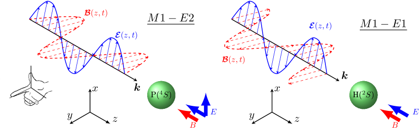
Figure 1: Principal scheme of experiments in which M1–E2 and M1–E1 ITs could be observed. Left: M1–E2 experiment with phosphorus atoms. No phase shift between electric ($\bm{\mathcal{E}}(z,t)$) and magnetic ($\bm{\mathcal{B}}(z,t)$) fields of radiation, static electric field $E$ has two components. Right: M1–E1 experiment with hydrogen atoms. There is a phase shift between electric and magnetic fields.

It may be, for example, the phosphorous atom at the transition $3s^{2}3p^{3}[X^{4}\!S^{\circ}_{3/2}-^{2}\!\!D^{\circ}_{\circ}]$ near 880 nm, which has emission inverse lifetimes of $1.77\times 10^{-4}$ and $1.2\times 10^{-4}$ s^-1 for M1- and E2-components, respectively[21]. Note that the $X^{4}S^{\circ}_{3/2}$ state is the ground state of the atom, this fact facilitates experimental preparation of the atom.

3.2 Phase shift between $\bm{\mathcal{E}}$ and $\bm{\mathcal{B}}$

Table 2 is not the end of a story. Equations (5–7) tell us, that the phase shift $\Delta\phi$ between electric wave $\bm{\mathcal{E}}$ and magnetic wave $\bm{\mathcal{B}}$ of light far from the source of the light (antenna) is zero, $\Delta\phi=0$.

However, the phase shift $\Delta\phi$ vary with distance between antenna and observation point. Close to the antenna, $|\Delta\phi|\approx\pi/2$. As the distance from the antenna increases, the phase $\Delta\phi$ decreases. This is the basic principle which is used today in near-field electromagnetic ranging (NFER) technology.

Moreover, in electron paramagnetic resonance (EPR) the microwave resonator is used, where electric and magnetic field components are exactly out of phase, $|\Delta\phi|=\pi/2$.

Therefore, if one uses such out-of-phase radiation, all the E-M interactions in Table 2 should be multiplied by imaginary unit $i$.

3.3 E1-M1

If EPR microwave resonator is available, observation of IT between M1- and E1-transitions becomes possible. In order to observe them, one should orient both the magnetic moment and the dipole moment of the atom along axis $z$, see fig. 1.

The simplest system here is probably hydrogen atom H(${}^{2}\!S$). With these two orientations, very simplified wave functions of the initial and the final states of the atom becomes

$$\Psi_{i} = a\Psi(^{2}\!S,-1/2)+b\Psi(^{2}\!P,-1/2),$$

$$\Psi_{f} = a^{\prime}\Psi(^{2}\!S,1/2)+b^{\prime}\Psi(^{2}\!P,1/2),$$

where we denoted $(^{2}\!S,\pm 1/2)\equiv(1s[^{2}\!S],m_{z}=\pm 1/2)$, $(^{2}\!P,\pm 1/2)\equiv$ $(2p[^{2}\!P_{1/2,3/2}]$, $m_{z}=\pm 1/2)$, and $a$, $b$, $a^{\prime}$, and $b^{\prime}$ are real coefficients. In reality, orientation of atom by constant electric field produces a sum of different antisymmetric states of the same parity, not only $2p[^{2}P]$.

In order to increase population difference between two Zeeman-split $m_{z}=\pm 1/2$ sublevels, low temperature should be employed. Here for simplicity we assume so low temperatures, that contribution of $|1s[^{2}S],m_{z}=+1/2>$ state to $\Psi_{i}$ is negligible.

The IT may be calculated as:

$$\!\!({\bm{d}}\cdot\bm{\mathcal{E}})_{fi}({\bm{\mu}}\cdot\bm{\mathcal{B}})_{fi}\! \!=\! \!\mathcal{E}_{x}\!\left[ab^{\prime}\langle^{2}\!P,\frac{1}{2}|d_{x}|^{2}\!S,-\frac{1}{2}\rangle+ba^{\prime}\langle^{2}\!S,\frac{1}{2}|d_{x}|^{2}\!P,-\frac{1}{2}\rangle\right]\times$$ (12)

$$\!\times\! \!\mathcal{B}_{y}\!\left[aa^{\prime}\langle^{2}\!S,\frac{1}{2}|i\mu_{y}|^{2}\!S,-\frac{1}{2}\rangle+bb^{\prime}\langle^{2}\!P,\frac{1}{2}|i\mu_{y}|^{2}\!P,-\frac{1}{2}\rangle\right]\!,$$

where $\mathcal{E}_{x}$ and $\mathcal{B}_{y}$ are real values.

Important, that this expression is real, this fact makes it possible to contribute to E1- and M1- transitions, which are proportional to $\mathcal{E}^{2}_{x}|{\bm{d}}_{fi}|^{2}$ and $\mathcal{B}_{y}^{2}|{\bm{\mu}}_{fi}|^{2}$, respectively.

4 Analytical summation of multipole series

Summarizing operators for multipole interactions from Table 1, we receive a new method for calculation of light-molecule interactions, which does not require the summation of endless series (3):

$$\frac{W_{i\to f}}{C}=|V^{Eo}_{fi}|^{2}+|V^{Ee}_{fi}|^{2}+|V^{Mo}_{fi}|^{2}+|V^{Me}_{fi}|^{2},$$ (13)

where

$$V^{Eo} \equiv \sum_{n=0}^{\infty}\hat{\mathcal{V}}^{(E2n+1)}=e\frac{\sin\theta}{\theta}\;({\bm{r}}\cdot\bm{\mathcal{E}}),$$ (14)

$$V^{Ee} \equiv \sum_{n=1}^{\infty}\hat{\mathcal{V}}^{(E2n)}=ie\frac{(1-\cos\theta)}{\theta}\;({\bm{r}}\cdot\bm{\mathcal{E}}),$$ (15)

$$V^{Mo} \equiv \sum_{n=0}^{\infty}\hat{\mathcal{V}}^{(M2n+1)}=\mu_{B}\left[\frac{2(\cos\theta+\theta\sin\theta-1)}{\theta^{2}}\hat{\bm{L}}+\right.$$ (16)

$$+ \left.\cos\theta\;g_{e}\hat{\bm{S}}\right]\cdot\bm{\mathcal{B}},$$

$$V^{Me} \equiv \sum_{n=1}^{\infty}\hat{\mathcal{V}}^{(M2n)}=i\mu_{B}\left[\frac{2(\sin\theta-\theta\cos\theta)}{\theta^{2}}\hat{\bm{L}}+\right.$$ (17)

$$+ \left.\sin\theta\;g_{e}\hat{\bm{S}}\right]\cdot\bm{\mathcal{B}}.$$

If necessary, both $V^{M}$ expressions may be easily transformed to hermetian form via replacing of $f(\theta)\hat{{\bm{L}}}$ by $[f(\theta)\hat{{\bm{L}}}+\hat{{\bm{L}}}f(\theta)]/2$, where $f(\theta)$ denote expressions before ${\bm{L}}$ in Eqs. (16) and (17).

It is well known that calculations of truncated Taylor expansion (1) may lead to wrong results. According to George et al., ”…the calculated E2- and M1-transition probabilities may grow to arbitrarily large values depending on the position of the coordinates origin”[3].

If one uses our expressions (13), it is evident, that the ”origin problem” probably remains, but large values of transition probabilities cannot appear, because all the functions of variable $\theta$ quickly decrease with $\theta$.

5 Results and conclusions

In summary, we classified the obstacles which prevent observation of interference terms. These terms arise in the calculation of light-matter interactions, if these interactions are presented as a series of interactions between multipole moments of the system (atom or molecule) and electric or magnetic fields of the probe electromagnetic radiation, see Table 1.

Some of these obstacles are shown to be overcomable, see Table 2, and we pointed out the ways, how to do it. Thus, orientation of atoms (or molecules) should be used and, in some cases — appropriate phase shift between electric and magnetic fields of the probe radiation. As a result, we proposed experimental schemes which could be used to observe E1-M1 and E2-M1 interference terms.

Also, we propose simple analytical expression (13) for light-matter interactions to be used instead of the series of multipole interactions and interferences between them. Hopefully, this expression will find application in the X-ray spectroscopy.

References

• [1] L.ย D. Barron. Molecular Light Scattering and Optical Activity. Cambridge University Press, Cambridge, 2 edition, 2004.
• [2] R.ย E. Raab and O.ย L. deย Lange. Multipole Theory In Electromagnetism: Classical, Quantum, And Symmetry Aspects, With Applications. Oxford University Press, Oxford, 2005.
• [3] S.ย DeBeerย George, T.ย Petrenko, and F.ย Neese. Time-dependent density functional calculations of ligand K-edge X-ray absorption spectra. Inorg. Chim. Acta, 361:965โ€“972, 2008.
• [4] Stephan Bernadotte, Andrewย J. Atkins, and Christophย R. Jacob. Origin-independent calculation of quadrupole intensities in X-ray spectroscopy. J. Chem. Phys., 137(20):204106, 2012.
• [5] Patrickย J. Lestrange, Franco Egidi, and Xiaosong Li. The consequences of improperly describing oscillator strengths beyond the electric dipole approximation. J. Chem. Phys., 143(23):234103, 2015.
• [6] U.I. Safronova, A.S. Safronova, S.M. Hamasha, and P.ย Beiersdorfer. Relativistic many-body calculations of multipole (E1, M1, E2, M2, E3, and M3) transition wavelengths and rates between $3l^{-1}4l^{\prime}$ excited and ground states in nickel-like ions. Atomic Data and Nuclear Data Tables, 92(1):47 โ€“ 104, 2006.
• [7] J.E. Allan. A spectral interference in atomic absorption spectroscopy. Spectrochimica Acta Part B: Atomic Spectroscopy, 24(1):13 โ€“ 18, 1969.
• [8] H[elene] Lefebvre-Brion and R[obert]ย W. Field. The spectra and dynamics of diatomic molecules. Elsevier Academic Press, Amsterdam, 2004.
• [9] R.E. Raab. Magnetic multipole moments. Mol. Phys., 29:1323โ€“1331, 1975.
• [10] H.ย J. Loesch and J.ย Remscheid. Brute force in molecular reaction dynamics: A novel technique for measuring steric effects. J. Chem. Phys., 93:4779, 1990.
• [11] L.ย Holmegaard, J.ย L. Hansen, L.ย Kalhoj, S.ย L. Kragh, H.ย Stapelfeldt, F.ย Filsinger, J.ย Kupper, G.ย Meijer, D.ย Dimitrovski, M.ย Abu-samha, C.ย P.ย J. Martiny, and L.ย B. Madsen. Photoelectron angular distributions from strong - field ionization of oriented molecules. Nature Phys., 6:428โ€“432, 2010.
• [12] Henrik Stapelfeldt and Tamar Seideman. Colloquium: Aligning molecules with strong laser pulses. Rev. Mod. Phys., 75:543โ€“557, Apr 2003.
• [13] Isabell Thomann, Robynne Lock, Vandana Sharma, Etienne Gagnon, Stephenย T. Pratt, Henryย C. Kapteyn, Margaretย M. Murnane, and Wen Li. Direct measurement of the angular dependence of the single-photon ionization of aligned N2 and CO2. J. Phys. Chem. A, 112(39):9382, 2008.
• [14] A.ย Goban, S.ย Minemoto, and H.ย Sakai. Laser -field-free molecular orientation. Phys. Rev. Lett., 101:013001, 2008.
• [15] S.ย De, I.ย Znakovskaya, D.ย Ray, F.ย Anis, Noraย G. Johnson, I.ย A. Bocharova, M.ย Magrakvelidze, B.ย D. Esry, C.ย L. Cocke, I.ย V. Litvinyuk, and M.ย F. Kling. Field -free orientation of co molecules by femtosecond two -color laser fields. Phys. Rev. Lett., 103:153002, 2009.
• [16] B.ย Friedrich and D.ย Herschbach. Manipulating molecules via combined static and laser fields. J. Phys. Chem. A, 103:10280, 1999.
• [17] O.ย Ghafur, A.ย Rouzee, A.ย Gijsbertsen, W.ย K. Siu, S.ย Stolte, and M.ย J.ย J. Vrakking. Impulsive orientation and alignment of quantum-state -selected no molecules. Nature Phys., 5:289 โ€“293, 2009.
• [18] Jonasย L. Hansen, Juanย J. Omiste, Jensย H. Nielsen, Dominik Pentlehner, Jochen Kupper, Rosario Gonzalez-Ferez, and Henrik Stapelfeldt. Mixed-field orientation of molecules without rotational symmetry. J. Chem. Phys., 139(23):234313, 2013.
• [19] A.ย R.ย W. McKellar. Laser magnetic resonance spectrum of BrO (ฮ 1/22superscriptsubscriptฮ 122{}^{2}\Pi_{1/2} $\rightarrow$ ฮ 3/22superscriptsubscriptฮ 322{}^{2}\Pi_{3/2}). J. Molec. Spectr., 86(1):43โ€“54, 1981.
• [20] D.ย A. Varshalovich, A.ย N. Moskalev, and V.ย K. Khersonskii. Quantum theory of angular momemtum. World Scientific, Singapore, 1988.
• [21] A.ย Kramida, Yu.ย Ralchenko, J.ย Reader, and and NIST ASD Team. NIST Atomic Spectra Database (ver. 5.5.6), [Online]. Available: https://physics.nist.gov/asd [2018, August 16]. National Institute of Standards and Technology, Gaithersburg, MD., 2018.