Stein-type covariance identities:
Klaassen, Papathanasiou and Olkin-Shepp–type bounds for arbitrary target distributions

Abstract

In this paper, following on from [49, 50, 63] we present a minimal formalism for Stein operators which leads to different probabilistic representations of solutions to Stein equations. These in turn provide a wide family of Stein-Covariance identities which we put to use for revisiting the very classical topic of bounding the variance of functionals of random variables. Applying the Cauchy-Schwarz inequality yields first order upper and lower Klaassen [45]-type variance bounds. A probabilistic representation of Lagrange’s identity (i.e. Cauchy-Schwarz with remainder) leads to Papathanasiou [60]-type variance expansions of arbitrary order. A matrix Cauchy-Schwarz inequality leads to Olkin-Shepp [59] type covariance bounds. All results hold for univariate target distribution under very weak assumptions (in particular they hold for continuous and discrete distributions alike). Many concrete illustrations are provided.

1 Introduction

Charles Stein’s mathematical legacy is growing at a remarkable pace and many of the techniques and concepts he pioneered are now a staple of contemporary probability theory. The origins of this stream of research lie in two papers: [67], in which the method was first presented in the context of Gaussian approximation, and [20] where the method was first adapted to a non-Gaussian context, namely that of Poisson approximation. As has been noted by many authors since then, the approach can be applied quasi verbatim to any target distribution other than the Gaussian and the Poisson, under the condition that “correct” ad hoc objects be identified which will permit the basic identities to hold. There now exist several excellent books and reviews on Stein’s method and its consequences in various settings, such as [68, 9, 10, 57, 21]. There also exist several non-equivalent general frameworks for the theory covering to large swaths of probability distributions, of which we single out the works [26, 70] for univariate distributions under analytical assumptions, [6, 7] for infinitely divisible distributions and [55, 35, 37] as well as [29] for multivariate densities under diffusive assumptions. A “canonical” differential Stein operator theory is also presented in [49, 50, 63].

Stein’s method can be broken down into a small number of key steps: [A] identification of a (characterizing) linear operator, [B] bounding of solutions to some differential equations related to this operator, [C] probabilistic Taylor expansions and construction of well-designed couplings; see [62] for an overview. Each of these steps has produced an entire ecosystem of “Stein-type objects” (operators, equations, couplings, etc.). These Stein-type objects are in symbiosis with many classical branches of mathematics such as orthogonal polynomials, functional analysis, PDE theory or Markov chain theory and therefore open bridges between Stein’s theory and these important areas of mathematics. More recently, connections with other more contemporary mathematics have been discovered, such as e.g. information theory as in [58, 8], optimal transportation as in [48, 31], and machine learning as in [36, 53, 23].

In the present paper, we pursue the work begun in [49, 50, 63] and adopt a minimal point of view on all the objects concerned, this time concentrating on the solutions to so-called “Stein equations”. Aside from its intrinsic interest – which may arguably be only of concern to those meddling directly in the method itself – we shall illustrate the power of our formalism by showing how it allows to obtain optimal and (extremely) flexible upper and lower bounds on arbitrary functionals of random variables with arbitrary univariate distribution. We recover, as particular cases, many (all?) previously known “variance bounds” (also called Poincaré inequalities), including Klaassen’s bounds from [45], Papathanasiou’s variance expansions from [60] (and Houdré and Kagan’s famous expansion from [39]) as well as Olkin and Shepp’s bound from [59]. Our method of proof is in each case new and, moreover, the formalism we introduce makes them in some sense elementary – at least as soon as the framework is laid out. In order to ease the reader into our work, we begin by detailing it in the easiest setting, namely that of a Gaussian target distribution.

1.1 The Gaussian case

The Gaussian density $\gamma(x)=(2\pi\sigma^{2})^{-1/2}\mathrm{exp}(-(x-\mu)^{2}/2\sigma^{2})$ has many remarkable properties. One of them stems from Stein’s celebrated lemma which reads: a random variable $N$ has distribution $N\sim\mathcal{N}(\mu,\sigma^{2})$ if and only if

$$\mathbb{E}\left[(N-\mu)g(N)\right]=\mathbb{E}\left[\sigma^{2}g^{\prime}(N)\right]$$ (1.1)

$\mbox{for all }g:{\rm I\kern-1.60004ptR}\to{\rm I\kern-1.60004ptR}\mbox{ such that }\mathbb{E}[|g^{\prime}(N)|]<\infty.$ We let $\mathcal{F}(\gamma)$ be the collection of $g$ such that $\mathbb{E}|g^{\prime}(N)|<\infty$. There are many ways to prove (1.1), but the two basic approaches are:

• Approach 1: use the fact that the Gaussian score function $\rho(x)=(\log\gamma(x))^{\prime}=\gamma^{\prime}(x)/\gamma(x)=-(x-\mu)/\sigma^{2}$ is linear, in combination with integration by parts (see [69]);

• Approach 2: use the fact that the Gaussian Stein kernel $\tau(x)=\gamma(x)^{-1}\int_{-\infty}^{x}(u-\mu)\gamma(u)du=\sigma^{2}$ is constant, in combination with Fubini’s theorem (see [57, Lemma 1.2]).

Contrarily to appearances, the final result obtained via these two approaches is not identical because (i) there are technical differences concerning the classes of test functions to which the resulting identities apply; (ii) they lead to two formally different identities: where the variance is on the right-hand-side of the equality (1.1) via Approach 2, it is at the denominator of the left hand side of the equality via Approach 1. This is not a simple cosmetic difference that can be brushed away as a byproduct of the standardization, it is rather central to the understanding of the very nature of Stein’s operators and the innocuity of the difference is rather characteristic of the Gaussian distribution. In the language of the present paper, many of the remarkable properties of the Gaussian actually stem from a very “Steinian” characteristic property of the Gaussian: it is the only distribution whose Stein kernel $\tau(x)=\gamma(x)^{-1}\int_{-\infty}^{x}(u-\mu)\gamma(u)du$ is constant.

In order to exploit Stein’s identity (1.1) in the context of the so-called Stein’s method, one starts by considering solutions to the so-called Stein equations

$$\sigma^{2}f_{h}^{\prime}(x)-(x-\mu)f_{h}(x)=h(x)-\mathbb{E}[h(N)]$$ (1.2)

where $h\in\mathcal{H}$ some class of test functions. For any given $h\in L^{1}(\gamma)$ there exists (a.s.) a unique solution $\mathcal{L}_{\gamma}h=f_{h}$ to (1.2) such that $f_{h}$ is bounded on ${\rm I\kern-1.60004ptR}$, given by

$$\mathcal{L}_{\gamma}h(x)=f_{h}(x)=\frac{1}{\gamma(x)}\int_{-\infty}^{x}\big{(}h(u)-\mathbb{E}[h(N)]\big{)}\gamma(u)du=-\frac{1}{\gamma(x)}\int_{x}^{\infty}\big{(}h(u)-\mathbb{E}[h(N)]\big{)}\gamma(u)du.$$ (1.3)

The operator $h\mapsto\mathcal{L}_{\gamma}h$ is called the pseudo inverse Stein operator. Such functions as (1.3) can be used in order to assess normality of a real valued random variable $X$ through the identities:

$$\sup_{h{\in}\mathcal{H}}\mathbb{E}[h(X)]-\mathbb{E}[h(N)] =\sup_{h\in\mathcal{H}}\mathbb{E}[\sigma^{2}f_{h}^{\prime}(X)-(X-\mu)f_{h}(X)]$$ (1.4)

$$\leq\sup_{f\in\mathcal{F}}\mathbb{E}[\sigma^{2}f^{\prime}(X)-(X-\mu)f(X)]$$ (1.5)

where $\mathcal{F}\supset\left\{\mathcal{L}_{\gamma}h\,|\,h\in\mathcal{H}\right\}$ is to be “well-chosen”. The expressions on the left hand side of (1.4) are classical, as they correspond to the so-called Integral Probability Metric (IPM): Wasserstein-1 distance for $\mathcal{H}_{\mathrm{Lip}}=$Lip(1) the class of all Lipschitz functions with constant 1; Total Variation distance for $\mathcal{H}_{TV}=\left\{\mathbb{I}_{A},A\subset{\rm I\kern-1.60004ptR}\right\}$ the class of all indicators of all Borel sets in ${\rm I\kern-1.60004ptR}$; Kolmogorov distance for $\mathcal{H}_{\mathrm{Kol}}=\left\{\mathbb{I}_{(-\infty,z]},z\in{\rm I\kern-1.60004ptR}\right\}$ the class of indicators of half lines. These are natural measures of probabilistic discrepancy. The right hand side of (1.5) is more mysterious, and one of the secrets of its usefulness lies in the fact that one can chose the class $\mathcal{F}$ to be of a very simple nature. Indeed, we start with the observation that there exist constants $\kappa^{i}_{\mathcal{H}},i=1,2,\ldots$ such that the functions $f_{h}$ satisfy the uniform bounds

$$\sup_{h\in\mathcal{H}}\|f_{h}\|_{\infty}\leq\kappa^{1}_{\mathcal{H}},\quad\sup_{h\in\mathcal{H}}\|f_{h}^{\prime}\|_{\infty}\leq\kappa_{\mathcal{H}}^{2},\quad\sup_{h\in\mathcal{H}}\|f_{h}^{\prime\prime}\|_{\infty}\leq\kappa_{\mathcal{H}}^{3}\quad\ldots$$ (1.6)

for all important classes $\mathcal{H}$ (including the three mentioned above) – these are the so-called “Stein’s factors”. Given bounds such as (1.6) one can take

$$\mathcal{F}=\left\{f:{\rm I\kern-1.60004ptR}\to R\mbox{ such that }\|f\|_{\infty}\leq\kappa_{\mathcal{H}}^{1},\|f^{\prime}\|_{\infty}\leq\kappa_{\mathcal{H}}^{2},\mbox{ etc}\right\}$$ (1.7)

so that $\mathcal{F}\supset\left\{f_{h}\mbox{ of the form \eqref{eq:58}}\right\}$ and, crucially, the class $\mathcal{F}$ has a simple structure. This makes (1.5) a very potent starting point for assessing normality of $X$.

Starting from (1.1), it is natural to consider the Stein operator $\mathcal{A}_{\gamma}f(x)=\sigma^{2}f^{\prime}(x)-(x-\mu)f(x)$ which has the property that $X=N$ (equality in distribution) if and only if $\mathbb{E}[\mathcal{A}_{\gamma}f(N)]=0$ for all $f\in\mathcal{F}(\gamma)$. In light of the arguments from the previous paragraph, the inverse of $\mathcal{A}_{\gamma}$ is given by the pseudo inverse Stein operator which is the integral operator which to any $h\in L^{1}(\gamma)$ associates the function $\mathcal{L}_{\gamma}h$ given in (1.3). With this construction, $\mathcal{A}_{\gamma}\mathcal{L}_{\gamma}h=h-\mathbb{E}[h[N]]$ for all $h\in L^{1}(\gamma)$ and $\mathcal{L}_{\gamma}\mathcal{A}_{\gamma}h=h$ for all $h\in\mathcal{F}(\gamma)$.

Here are some important examples. With $g_{z}(x)=\mathbb{I}(x\leq z),$

$$\mathcal{L}_{\gamma}g_{z}(x)=\frac{1}{\gamma(x)}\left(\mathbb{P}(N\leq x\wedge z)-\mathbb{P}(N\leq x)\mathbb{P}(N\leq z)\right).$$ (1.8)

As a second example, the Stein kernel $\tau(x)$ is nothing other than the solution (1.3) evaluated at $h=\mathrm{Id}$ the identity function; $\mathcal{L}_{\gamma}\mathrm{Id}(x)=\tau(x)$ which, as already mentioned, is constant and equal to $\sigma^{2}$ at all $x$. From Stein’s identity we deduce that the Gaussian density is the only density for which the function $\mathcal{L}_{\gamma}\mathrm{Id}$ is constant. The operator $\mathcal{L}_{\gamma}$ evaluated at the identity function in general gives the zero bias density from [33], in the sense that $\mathbb{E}[Xh(X)]=\mathbb{E}[\{-\mathcal{L}_{\gamma}\mathrm{Id}(X)\}h^{\prime}(X)]=\mathbb{E}[h^{\prime}(X^{*})]$, with $X^{*}$ having the $X$-zero bias density.

The Stein operator definition gives in particular that, for $f\in\mathcal{F}(\gamma)$ and $h\in L^{1}(\gamma)$,

$$\mathbb{E}\left[\{\mathcal{A}_{\gamma}f(N)\}h(N)\right]=\sigma^{2}\mathbb{E}[f^{\prime}(N)h(N)-(fh)^{\prime}(N)]=-\mathbb{E}[f(N)h^{\prime}(N)].$$

Letting $g(x)=\mathcal{A}_{\gamma}f(x)$ and using $\mathcal{L}_{\gamma}\mathcal{A}_{\gamma}h=h$ allows to generalize (1.1) to the covariance identity:

$$\mathrm{Cov}\left[g(N),h(N)\right]=\mathbb{E}\left[\big{(}-\mathcal{L}_{\gamma}g(N)\big{)}\,h^{\prime}(N)\right]$$ (1.9)

which is valid for all $h,g\in L^{1}(\gamma)$. For further covariance inequalities we start with the (trivial) observation that

$$\mathcal{L}_{\gamma}h(x)=\frac{1}{\gamma(x)}\mathbb{E}\left[\big{(}h(N)-\mathbb{E}[h(N)]\big{)}\mathbb{I}[N\leq x]\right]=\mbox{Cov}\bigg{[}h(N),\frac{\mathbb{I}[N\leq x]}{\gamma(x)}\bigg{]}.$$ (1.10)

Then the following holds.

Lemma 1.1 (Representation of the inverse Stein operator).

Let $N_{1},N_{2}$ be independent copies of $N$. Then

$$-\mathcal{L}_{\gamma}h(x)=\frac{1}{\gamma(x)}\mathbb{E}\left[\big{(}h(N_{2})-h(N_{1})\big{)}\mathbb{I}[N_{1}\leq x\leq N_{2}]\right]$$ (1.11)

for all $h\in L^{1}(\gamma)$.

The proof of Lemma 1.1 follows simply by expanding (1.11) and showing that it is equal to (1.10) for all $x$. We will provide details in a (much) more general context in Section 4 (see Lemma 4.1).

Identity (1.11) is not the only available probabilistic representation for $\mathcal{L}_{\gamma}$. The next one we found in [64, Proposition 1].

Lemma 1.2 (Saumard’s lemma).

The symmetric kernel

$$K_{\gamma}(x,x^{\prime})=\mathbb{P}[N\leq x\wedge x^{\prime}]-\mathbb{P}[N\leq x]\mathbb{P}[N\leq x^{\prime}]$$ (1.12)

is positive definite. Moreover

$$-\mathcal{L}_{\gamma}h(x)=\mathbb{E}\left[h^{\prime}(N)\frac{K_{\gamma}(N,x)}{\gamma(N)\gamma(x)}\right]$$ (1.13)

for all absolutely continuous $h\in L^{1}(\gamma)$, and letting $N_{1},N_{2}$ be independent copies of $N$ we have

$$\mathrm{Cov}[h(N),g(N)]=\mathbb{E}\left[h^{\prime}(N_{1})\frac{K_{\gamma}(N_{1},N_{2})}{\gamma(N_{1})\gamma(N_{2})}g^{\prime}(N_{2})\right]$$ (1.14)

for all absolutely continuous $h,g\in L^{2}(\gamma)$.

Remark 1.1.

Functions $x^{\prime}\mapsto K_{\gamma}(x,x^{\prime})/\gamma(x^{\prime})$ are represented in Figure 1(a) for various values of $x$.

Proof.

Symmetry of (1.12) is immediate. To see that it is positive, we note that

$$K_{\gamma}(x,x^{\prime})=\begin{cases}\mathbb{P}[N\leq x]\mathbb{P}[N\geq x^{\prime}]&\mbox{ if }x\leq x^{\prime}\\ \mathbb{P}[N\leq x^{\prime}]\mathbb{P}[N\geq x]&\mbox{ if }x>x^{\prime}\end{cases}.$$

To obtain (1.13), we use (1.9) inside (1.10): recalling the notation $g_{x}(n)=\mathbb{I}[n\leq x]$ we have

$$-\mathcal{L}_{\gamma}h(x) =\frac{1}{\gamma(x)}\mathrm{Cov}\left[h(N),g_{x}(N)\right]=\frac{1}{\gamma(x)}\mathbb{E}\left[h^{\prime}(N)\big{(}-\mathcal{L}_{\gamma}g_{x}(N))\right].$$

Using (1.8), with $N^{\prime}$ an independent copy of $N$,

$$-\mathcal{L}_{\gamma}g_{x}(N)=\frac{1}{\gamma(N)}\left(\mathbb{P}(N^{\prime}\leq x\wedge N)-\mathbb{P}(N^{\prime}\leq x)\mathbb{P}(N^{\prime}\leq N)\right).$$

Hence

$$-\mathcal{L}_{\gamma}h(x) =\mathbb{E}\left[\frac{1}{\gamma(x)\gamma(N)}\left(\mathbb{P}(N^{\prime}\leq x\wedge N)-\mathbb{P}(N^{\prime}\leq x)\mathbb{P}(N^{\prime}\leq N)\right)h^{\prime}(N)\right]$$

and (1.13) follows. For the last point, we simply combine (1.9) and (1.13) again, with $N_{2}$ yet another independent copy of $N$. Then

$$\mathrm{Cov}[h(N),g(N)] =\mathbb{E}\left[h^{\prime}(N_{1})\big{(}-\mathcal{L}_{\gamma}g(N_{1})\big{)}\right]=\mathbb{E}\left[h^{\prime}(N_{1})\mathbb{E}\bigg{[}g^{\prime}(N_{2})\frac{K_{\gamma}(N_{1},N_{2})}{\gamma(N_{1})\gamma(N_{2})}\,|\,N_{1}\bigg{]}\right]$$

and the conclusion follows. ∎

We conclude this introduction by showing how the notations we have introduced are not only of cosmetic value, but that they allow to obtain some powerful results in an efficient manner. For instance, starting from Saumard’s lemma combined with a simple application of the Cauchy-Schwarz inequality, for any test function such that $h^{\prime}>0$ a.s. then

$$\mathrm{Var}[g(N)] =\mathbb{E}\left[g^{\prime}(N_{1})\frac{K_{\gamma}(N_{1},N_{2})}{\gamma(N_{1})\gamma(N_{2})}g^{\prime}(N_{2})\right]$$

$$=\mathbb{E}\left[\frac{g^{\prime}(N_{1})}{\sqrt{h^{\prime}(N_{1})}}\sqrt{\frac{K_{\gamma}(N_{1},N_{2})h^{\prime}(N_{2})}{\gamma(N_{1})\gamma(N_{2})}}\sqrt{\frac{K_{\gamma}(N_{1},N_{2})h^{\prime}(N_{1})}{\gamma(N_{1})\gamma(N_{2})}}\frac{g^{\prime}(N_{2})}{\sqrt{h^{\prime}(N_{2})}}\right]$$

$$\leq\mathbb{E}\left[\frac{g^{\prime}(N_{1}))^{2}}{h^{\prime}(N_{1})}\frac{K_{\gamma}(N_{1},N_{2})h^{\prime}(N_{2})}{\gamma(N_{1})\gamma(N_{2})}\right]$$

$$=\mathbb{E}\left[\frac{g^{\prime}(N_{1}))^{2}}{h^{\prime}(N_{1})}\mathbb{E}\left[\frac{K_{\gamma}(N_{1},N_{2})h^{\prime}(N_{2})}{\gamma(N_{1})\gamma(N_{2})}\,\bigg{|}\,N_{1}\right]\right]=\mathbb{E}\left[\frac{g^{\prime}(N_{1}))^{2}}{h^{\prime}(N_{1})}\big{(}-\mathcal{L}_{\gamma}h(N_{1})\big{)}\right]$$

where we applied (1.13) once again. Lower bounds are just as easy to obtain, from (1.9):

$$\mathbb{E}\left[\big{(}-\mathcal{L}_{\gamma}h(N)\big{)}g^{\prime}(N)\right]^{2}\leq\mathbb{E}[h(N)^{2}]\mathrm{Var}[g(N)]$$

which leads to the fact that, if $h\in L^{1}(\gamma)$ is monotone, then

$$\frac{\mathbb{E}\left[\big{(}-\mathcal{L}_{\gamma}h(N)\big{)}g^{\prime}(N)^{2}\right]}{\mathbb{E}[h(N)^{2}]}\leq\mathrm{Var}[g(N)]\leq\mathbb{E}\left[\left(\frac{g^{\prime}(N_{1}))^{2}}{h^{\prime}(N_{1})}\right)^{2}\big{(}-\mathcal{L}_{\gamma}h(N_{1})\big{)}\right].$$ (1.15)

In particular, taking $h=\mathrm{Id}$

$$\sigma^{2}\mathbb{E}[g^{\prime}(N)]^{2}\leq\mbox{Var}[g(X)]\leq\sigma^{2}\mathbb{E}[g^{\prime}(X)^{2}].$$ (1.16)

Identity (1.16) is a rephrasing of Chernoff [22]’s classical Gaussian bounds; identity (1.15) is Klaassen’s result [45] in the Gaussian case. As we shall see in Section 4, one can push the argumentation much further and obtain upper and lower infinite variance expansions to any order. In particular we recover the famous variance bound from [39] (which was already available in [60]): for all $n\geq 1$,

$$\sum_{j=1}^{2n}(-1)^{j}\frac{(\sigma^{2})^{j}}{j!}\mathbb{E}[(g^{(j)}(N))^{2}]\leq\mbox{Var}[g(N)]\leq\sum_{j=1}^{2n+1}(-1)^{j}\frac{(\sigma^{2})^{j}}{j!}\mathbb{E}[g^{(j)}(N)^{2}].$$ (1.17)

Moreover, we will prove in Section 5 the matrix variance bound:

$$\begin{pmatrix}\mathrm{Var}[f(X)]&\mathrm{Cov}[f(X),g(X)]\\ \mathrm{Cov}[f(X),g(X)]&\mathrm{Var}[g(X)]\end{pmatrix}\leq\sigma^{2}\begin{pmatrix}\mathbb{E}\left[\big{(}f^{\prime}(X)\big{)}^{2}\right]&\mathbb{E}\left[f^{\prime}(X)g^{\prime}(X)\right]\\ \mathbb{E}\left[f^{\prime}(X)g^{\prime}(X)\right]&\mathbb{E}\left[\big{(}g^{\prime}(X)\big{)}^{2}\right]\end{pmatrix}$$

(inequality in the above indicating that the difference is non negative definite), hereby recovering the main result of [59]. Again, our approach applies to basically any univariate target distribution.

1.2 Some references

Extensions of Chernoff’s first order bound (1.16) have, of course, attracted much attention. The initiators of the stream of research seem to be [18] and [13], although precursors can be found e.g. in [12]. Chen [18] identified a way to exploit Stein’s operator for the Gaussian distribution not only to simplify Chernoff’s proof, but also to propose a first order upper variance bound for the multivariate Gaussian distribution. [13] identifies the role played by the Stein kernel (and its discrete version) to extend the scope of Chernoff and Chen’s bounds to a very wide class of distributions. A remarkable generalization – and one of the main sources of inspiration behind the current article – is [45] who pinpoints the role plaid by Stein inverse operators in such bounds, and obtains the inequalities in (1.15) for virtually any functional of any univariate probability distribution. Other fundamental early contributions in this topic are [19], [15, 14], or [44] wherein various extensions are proposed (e.g. Karlin deals with the entire class of log-concave distributions). A major breakthrough is due to [60] who obtains infinite expansions for continuous targets, with coefficients very close in spirit to those that we shall propose in Section 4. Papathanasiou’s method of proof in [60] – which rests in an iterative rewriting of the exact remainder in the Cauchy Schwarz identity – is also a direct inspiration for ours. Such results open the way for a succesful line of research in connection with Pearson’s and Ord’s system of distributions including works such as [16], [46], [42], [61], and [17]. Similar results, by different means, are Houdré and Kagan’s famous arbitrary order bound (1.17) from [39], extended to wide families of targets e.g. in [41, 40]. The remarkable articles [25] and [47] both propose similar minded considerations in very general settings. More recently, the contributions [4], [5] [3] and [1] and [51, 52] begin to fully explore connections with Stein’s method. In the Gaussian framework, an enlightening first order matrix variance bound is proposed in [59] for the Gaussian distribution, and in a more general setting in [2] (and also to arbitrary order). Finally, we mention [66, 65] and [64]’s revisiting of this classical literature enticed us to begin the work that ultimately led to the present paper. We end this literature review by pointing to [24, 31, 30] wherein fundamental contributions to the theory of Stein kernels are provided in a multivariate setting.

1.3 Outline of the paper and main results

In Section 2 we recall the theory of canonical and standardized Stein operators introduced in [50], and adapt it to our present framework. We introduce a (new) notion of inverse Stein operator (Definition 2.3) along with a first representation formula (2.2); we also introduce one of the basic tools of the paper, namely a generalized indicator function (2.1) which will serve throughout the paper.

In Section 3 we present the main covariance identities (Lemmas 3.1, 3.2) along with a second probabilistic representation of the inverse operator in (3.7). The first variance Klaassen-type bounds are provided in Theorem 3.1. They take on the same exact form as (1.15). We stress that the method of proof is new, and elementary. Many standard examples are detailed.

Section 4 begins with a third probabilistic representation of the inverse operator in (4.2), which despite its simplicity seems to be new. A re-interpretation of the classical Lagrange identity is provided in Lemma 4.3, in our formalism; the basic building blocks of the theory are given in (4.1) and (4.7); these definitions are exactly the correct tool for obtaining general arbitrary order variance expansions detailed in Theorem 4.1. We identify in (4.14) fundamental “iterated Stein coefficients” which we denote $\Gamma_{k}^{\ell}(x)$; these generalize the classical Stein kernel and we give some abstract examples in Lemma 4.4, with concrete examples also provided for several classical targets. Section 5 details our extension of Olkin and Shepp’s first-order matrix variance-inequality “à la Klaassen”. The final section, Section 6, applies our framework to obtain bounds on solutions of Stein equations.

2 Stein differentiation

Let $\mathcal{X}\subset{\rm I\kern-1.60004ptR}$ and equip it with some $\sigma$-algebra $\mathcal{A}$ and $\sigma$-finite measure $\mu$. Let $X$ be a random variable on $\mathcal{X}$, with probability measure $P^{X}$ which is absolutely continuous with respect to $\mu$; we denote $p$ the corresponding density, and $\mathcal{S}(p)=\left\{x\in\mathcal{X}:p(x)>0\right\}$. Although we could in principle keep the discussion to come very general, in order to make the paper more concrete and readable in the sequel we shall restrict our attention to distributions satisfying the following assumption.

Assumption A. The measure $\mu$ is either the counting measure on $\mathcal{X}={\mathbb{Z}}$ or the Lebesgue measure on $\mathcal{X}={\rm I\kern-1.60004ptR}$. If $\mu$ is the counting measure then there exist $a,b\in{\mathbb{Z}}\cup\left\{-\infty,\infty\right\}$ such that $\mathcal{S}(p)=[a,b]\cap{\rm I\kern-1.60004ptN}$. If $\mu$ is the Lebesgue measure then $\overline{\mathcal{S}(p)}=[a,b]$ for $a,b\in{\rm I\kern-1.60004ptR}\cup\left\{-\infty,\infty\right\}$.

The necessary feature of Assumption A is that $\mu$ is translation-invariant; the assumption of compact support is made for convenience.

Let $\Delta^{\ell}f(x)=(f(x+\ell)-f(x))/\ell$ for all $\ell\in{\rm I\kern-1.60004ptR}$, with the convention that $\Delta^{0}f(x)=f^{\prime}(x)$, with $f^{\prime}(x)$ the weak derivative defined Lebesgue almost everywhere. We denote $\mathrm{dom}(p,\Delta^{\ell})$ the collection of functions $f:{\rm I\kern-1.60004ptR}\to{\rm I\kern-1.60004ptR}$ such that $\Delta^{\ell}f(x)$ exists and is finite at all $x\in\mathcal{S}(p)$. The next definitions come from [50].

Definition 2.1 (Canonical Stein operators).

Let $f\in\mathrm{dom}(p,\Delta^{\ell})$ and consider $\mathcal{T}_{p}^{\ell}f$ defined as $\mathcal{T}_{p}^{\ell}f(x)=\frac{\Delta^{\ell}(f(x)p(x))}{p(x)}$ for all $x\in\mathcal{S}(p)$ and $\mathcal{T}_{p}^{\ell}f(x)=0$ for $x\notin\mathcal{S}(p)$. Operator $\mathcal{T}_{p}^{\ell}$ is the canonical ($\ell$-)Stein operator of $p$. The cases $\ell=1$ and $\ell=-1$ provide the forward and backward Stein operators, denoted $\mathcal{T}_{p}^{+}$ and $\mathcal{T}_{p}^{-}$, respectively; the case $\ell=0$ provides the differential Stein operator denoted $\mathcal{T}_{p}$.

Definition 2.2 (Canonical Stein class).

We define $\mathcal{F}^{(0)}(p)$ as the class of functions in $L^{1}(p)$ which moreover have mean 0 with respect to $p$. The canonical $\ell$-Stein class of $p$ is the collection $\mathcal{F}^{(1)}_{\ell}(p)$ of $f:{\rm I\kern-1.60004ptR}\to{\rm I\kern-1.60004ptR}$ such that $x\mapsto f(x)p(x)\in\mathrm{dom}(p,\Delta^{\ell})$ and $\mathcal{T}_{p}^{\ell}f\in\mathcal{F}^{(0)}(p)$ (i.e. $\mathbb{E}\left[\mathcal{T}_{p}^{\ell}f(X)\right]=0$).

Remark 2.1.

For details on Stein class and operators, we refer to (i) [50] for the construction in an abstract setting, (ii) [49] for the construction in the continuous setting (i.e. $\ell=0$) and (iii) [28] for the construction in the discrete setting (i.e. $\ell\in\left\{-1,1\right\}$).

In what follows we restrict attention to the following cases: $\ell=0$ and $\mu$ is the Lebesgue measure; or $\ell\in\{-1,+1\}$ and $\mu$ is counting measure. We note that for positive integer $\ell$, we have $\Delta^{\ell}f(x)=\Delta^{1}\left(\frac{1}{\ell}\sum_{\ell=0}^{k-1}f(x+k)\right)$ and with this representation results for other integer values of $\ell$ could be obtained. For simplicity we do not consider this general case.

By definition, the canonical operators $\mathcal{T}_{p}^{\ell}$ embed $\mathcal{F}_{\ell}^{(1)}(p)$ into $\mathcal{F}^{(0)}(p)$ (and in particular $\mathbb{E}[\mathcal{T}_{p}^{\ell}f(X)]=0$ for all $f\in\mathcal{F}_{\ell}^{(1)}(p)$). Inverting this operation is an important part of the construction to come; the following result is well-known and easy to obtain.

Lemma 2.1 (Representation formula I).

Let $\ell\in\left\{-1,0,1\right\}$. Let $p$ with support $\mathcal{S}(p)$ satisfy Assumption A and define

$$\chi^{\ell}(x,y)=\mathbb{I}_{x\leq y-\ell(\ell+1)/2}.$$ (2.1)

Then for any $\eta\in\mathcal{F}^{(0)}(p)$, the function defined on $\mathcal{S}(p)$ as

$$\mathcal{L}^{\ell}_{p}\eta(x)=\frac{1}{p(x)}\mathbb{E}\left[\chi^{\ell}(X,x)\eta(X)\right]=\frac{1}{p(x)}\int\chi^{\ell}(y,x)\eta(y)p(y)d\mu(y)$$ (2.2)

satisfies (i) $\mathcal{L}^{\ell}_{p}\eta\in\mathcal{F}_{\ell}^{(1)}(p)$ and (ii) $\mathcal{T}_{p}^{\ell}\mathcal{L}^{\ell}_{p}\eta(x)=\eta(x)$ for all $x\in\mathcal{S}(p)$. If furthermore $\eta\in\mathcal{F}_{\ell}^{(1)}(p)$ then also $\mathcal{L}_{p}^{\ell}\mathcal{T}^{\ell}_{p}\eta(x)=\eta(x)$ for all $x\in\mathcal{S}(p)$.

Remark 2.2.

For $f\in{\rm{dom}}(p,\Delta^{\ell})$ such that $\mathbb{E}f(X)=0$ it holds that

$$\mathcal{L}^{\ell}_{p}f(x)=\frac{1}{p(x)}\mathbb{E}\left[\left(1-\chi^{\ell}(X,x)\right)f(X)\right]=\frac{1}{p(x)}\int\left(1-\chi^{\ell}(y,x)\right)f(y)p(y)d\mu(y).$$

Hence instead of Definition (2.1) in the developments below a more general version

$$\zeta^{\ell}(x,y)=\alpha\,\mathbb{I}_{x\leq y-\ell(\ell+1)/2}-\beta\,\mathbb{I}_{x>y-\ell(\ell+1)/2}$$

could be used, where $\alpha+\beta=1$. For simplicity we use Definition (2.1).

The expressions in Lemma 2.1 particularize, in the three cases that interest us, to $\chi^{-}(x,y)=\mathbb{I}_{x\leq y}$ $\big{(}\ell=-1\big{)}$, $\chi^{+}(x,y)=\mathbb{I}_{x<y}$ $\big{(}\ell=1\big{)}$ and $\chi^{0}(x,y)=\mathbb{I}_{x\leq y}$ $\big{(}\ell=0\big{)}$. If $\mu$ is the Lebesgue measure (and $\ell=0$) then

$$\mathcal{L}_{p}^{0}\eta(x)=\frac{1}{p(x)}\int_{a}^{x}\eta(u)p(u)du$$ (2.3)

whereas if $\mu$ is the counting measure then

$$\mathcal{L}_{p}^{+}\eta(x)=\frac{1}{p(x)}\sum_{j=a}^{x-1}\eta(j)p(j)\mbox{ }(\ell=1)\mbox{ and }\mathcal{L}_{p}^{-}\eta(x)=\frac{1}{p(x)}\sum_{j=a}^{x}\eta(j)p(j)\mbox{ }(\ell=-1).$$ (2.4)

In all cases the functions are extended on $\mathcal{X}$ through the convention that $\mathcal{L}_{p}^{\ell}\eta(x)=0$ for all $x\notin\mathcal{S}(p)$.

Definition 2.3 (Canonical pseudo inverse Stein operator).

The canonical pseudo-inverse Stein operator is

$$\mathcal{L}_{p}^{\ell}:L^{1}(p)\to\mathcal{F}^{(1)}_{\ell}(p):h\mapsto\mathcal{L}^{\ell}_{p}(h-\mathbb{E}[h(X)])$$ (2.5)

with $\mathcal{L}^{\ell}_{p}h(x)$ defined in Lemma 2.1.

Since the operators $\Delta^{\ell}$ satisfy the product rule $\Delta^{\ell}\big{(}f(x)g(x-\ell)\big{)}=\Delta^{\ell}f(x)g(x)+f(x)\Delta^{-\ell}g(x)$, we immediately obtain that $\mathcal{T}_{p}^{\ell}\big{(}f(x)g(x-\ell)\big{)}=\mathcal{T}_{p}^{\ell}f(x)g(x)+f(x)\Delta^{-\ell}g(x)$ for all appropriate $f,g$. This leads to

Definition 2.4 (Standardizations of the canonical operator).

Fix some $\eta\in\mathcal{F}^{(0)}(p)$. The $\eta$-standardized Stein operator is

$$\mathcal{A}_{p}g(x) =\mathcal{T}^{\ell}_{p}\big{(}\mathcal{L}^{\ell}_{p}\eta(\cdot)g(\cdot-\ell)\big{)}(x)=\eta(x)g(x)+\mathcal{L}^{\ell}_{p}\eta(x)\big{(}\Delta^{-\ell}g(x)\big{)}$$ (2.6)

acting on the collection $\mathcal{F}(\mathcal{A}_{p})$ of test functions $g$ such that $\eta(\cdot)g(\cdot-\ell)\in\mathcal{F}_{\ell}^{(1)}(p)$.

Example 2.1 (Binomial distribution).

Stein’s method for the binomial distribution was first developed in [27]. Let $p$ be the binomial density with parameters $(n,p)$. Then $\mathcal{S}(p)=[0,n]$, $\mathcal{F}_{+}^{(1)}(p)$ consists of bounded functions such that $f(0)=0$ and $\mathcal{F}_{-}^{(1)}(p)$ of functions such that $f(n)=0$. Picking $\ell=1$ and $\eta(x)=x-np$ then $\mathcal{L}_{n,p}^{+}\eta(x)=-(1-p)x$ so that

$$\mathcal{A}^{1}_{\mathrm{bin}(n,p)}g(x)=(x-np)g(x)-(1-p)x\Delta^{-}g(x)$$ (2.7)

with corresponding class $\mathcal{F}(\mathcal{A}_{\mathrm{bin}(n,p)})$ which contains all bounded functions $g:{\mathbb{Z}}\to{\rm I\kern-1.60004ptR}$. Picking $\ell=-1$ and $\eta(x)=x-np$ then $\mathcal{L}_{n,p}^{-}\eta(x)=-p(n-x)$ so that

$$\mathcal{A}^{2}_{\mathrm{bin}(n,p)}g(x)=(x-np)g(x)-p(n-x)\Delta^{+}g(x)$$ (2.8)

acting on the same class as (2.7).

Example 2.2 (Poisson distribution).

Stein’s method for the Poisson distribution originates in[20]. Let $p$ be the Poisson density with parameter $\lambda$. Then $\mathcal{S}(p)={\rm I\kern-1.60004ptN}$, $\mathcal{F}_{+}(p)$ consists of bounded functions such that $f(0)=0$ and $\mathcal{F}_{-}(p)$ of functions such that $\lim_{n\to\infty}f(n)\lambda^{n}/n!=0$. Picking $\ell=1$ and $\eta(x)=x-\lambda$ then $\mathcal{L}_{\lambda}^{+}\eta(x)=-x$ so that

$$\mathcal{A}^{1}_{\mathrm{Poi}(\lambda)}g(x)=(x-\lambda)g(x)-x\Delta^{-}g(x)$$ (2.9)

acting on $\mathcal{F}(\mathcal{A}^{1}_{\mathrm{Poi}(\lambda)})$ which contains all bounded functions $g:{\mathbb{Z}}\to{\rm I\kern-1.60004ptR}$. Picking $\ell=-1$ and $\eta(x)=x-\lambda$ then $\mathcal{L}_{\lambda}^{-}\eta(x)=-\lambda$ so that

$$\mathcal{A}^{2}_{\mathrm{Poi}(\lambda)}g(x)=(x-\lambda)g(x)-\lambda\Delta^{+}g(x)$$ (2.10)

acting on the same class as (2.9).

Example 2.3 (Beta distribution).

Let $p$ be the Beta density with parameters $(\alpha,\beta)$. Then $\mathcal{S}(p)=[0,1]$ and $\mathcal{F}(p)$ consists of functions such that $f(0)=f(1)=0$. If $\eta(x)=x-\alpha/(\alpha+\beta)$ then $\mathcal{L}_{\alpha,\beta}\eta(x)=-\frac{x(1-x)}{\alpha+\beta}$ leading to the operator

$$\mathcal{A}_{\mathrm{Beta}(\alpha,\beta)}g(x)=\Big{(}x-\frac{\alpha}{\alpha+\beta}\Big{)}g(x)-\frac{x(1-x)}{\alpha+\beta}g^{\prime}(x)$$ (2.11)

with corresponding class $\mathcal{F}(\mathcal{A}_{\mathrm{Beta}(\alpha,\beta)})$ which contains all differentiable, bounded functions $g:{\rm I\kern-1.60004ptR}\to{\rm I\kern-1.60004ptR}$; see [26] and [34] for more details and related Stein operators.

Example 2.4 (Gamma distribution).

Let $p$ be the gamma density with parameters $(\alpha,\beta)$. Then $\mathcal{S}(p)=(0,\infty)$ ($\alpha<1$) or $\mathcal{S}(p)=[0,\infty)$ ($\alpha\geq 1$) and $\mathcal{F}(p)$ consists of functions such that $f(0)=0$ all integrals exist. If $\eta(x)=x-\alpha\beta$ then $\mathcal{L}_{p}\eta(x)=-\beta x$ leading to the operator

$$\mathcal{A}_{\mathrm{gamma}(\alpha,\beta)}g(x)=\big{(}x-\alpha\beta\big{)}g(x)-\beta xg^{\prime}(x)$$ (2.12)

with corresponding class $\mathcal{F}(\mathcal{A}_{\mathrm{Gamma}(\alpha,\beta)})$ which contains all differentiable functions $g:{\rm I\kern-1.60004ptR}\to{\rm I\kern-1.60004ptR}$ such that the function $xg(x)$ is bounded; see for example [32] and [54] for more details and related Stein operators.

Example 2.5 (A general example).

Let $p$ satisfy Assumption A and suppose that it has finite mean $\mu$. If $\eta(x)=x-\mu$ then $\mathcal{L}_{p}\eta(x)=-\tau_{p}(x)$ is the so-called Stein kernel of $p$, leading to the operator

$$\mathcal{A}_{p}g(x)=\big{(}x-\mu\big{)}g(x)-\tau_{p}(x)g^{\prime}(x)$$ (2.13)

with corresponding class $\mathcal{F}(\mathcal{A}_{p})$ which contains all functions $g:{\rm I\kern-1.60004ptR}\to{\rm I\kern-1.60004ptR}$ such that $\tau_{p}g\in\mathcal{F}(p)$. Hence in the general case (2.6) can be viewed as generalisation of the Stein kernel. Implications of this observations are explored in detail in [28].

3 Stein covariance identities and Klaassen-type bounds

The construction from the previous sections is tailored to ensure that we easily deduce the following family of “Stein covariance identities” (e.g. use $\mathbb{E}[\mathcal{A}_{p}^{1}g(X)]=0$ for $\mathcal{A}_{p}^{1}$ as defined in (2.6)). Lemma 3.1 follows directly from the Stein product rule in [50, Theorem 3.24].

Lemma 3.1 (Stein IBP formulas).

Let $X\sim p$. Then, for all $c\in\mathcal{F}_{\ell}^{(1)}(p)$ on the one hand, and all $\eta\in\mathcal{F}^{(0)}(p)$ on the other hand, we have

$$\mathbb{E}\left[c(X)\Delta^{-\ell}g(X)\right]=-\mathbb{E}\left[{{\{}}\mathcal{T}_{p}^{\ell}c(X){{\}}}g(X)\right]$$ (3.1)

$$\mathbb{E}\left[-{{\{}}\mathcal{L}_{p}^{\ell}\eta(X){{\}}}\Delta^{-\ell}g(X)\right]=\mathbb{E}\left[\eta(X)g(X)\right]$$ (3.2)

for all $g$ such that $c(\cdot)g(\cdot-\ell)\in\mathcal{F}_{\ell}^{(1)}(p)$ (identity (3.1)) and all $g$ such that $\mathcal{L}_{p}^{\ell}\eta(\cdot)g(\cdot-\ell)\in\mathcal{F}_{\ell}^{(1)}(p)$ (identity (3.2)).

These identities provide powerful handles on the target distribution $X\sim p$. Combining them for instance with a second representation for Stein operator $\mathcal{L}_{p}^{\ell}$ given in (3.7) leads to the following result.

Lemma 3.2 (Representation formula II).

Define

$$K_{p}^{\ell}(x,x^{\prime})=\mathbb{E}[\chi^{\ell}(X,x)\chi^{\ell}(X,x^{\prime})\big{]}-\mathbb{E}[\chi^{\ell}(X,x)\big{]}\mathbb{E}\big{[}\chi^{\ell}(X,x^{\prime})\big{]}.$$ (3.3)

Then

$$\mathrm{Cov}[h(X),g(X)] =\mathbb{E}\bigg{[}-\mathcal{L}_{p}^{\ell}h(X)\Delta^{-\ell}g(X)\bigg{]}$$ (3.4)

$$=\mathbb{E}\left[\Delta^{-\ell}h(X)\frac{K_{p}^{\ell}(X,X^{\prime})}{p(X)p(X^{\prime})}\Delta^{-\ell}g(X^{\prime})\right]$$ (3.5)

$$\bigg{(}=\int_{\mathcal{S}(p)}\int_{\mathcal{S}(p)}\Delta^{-\ell}h(x)K_{p}^{\ell}(x,x^{\prime})\Delta^{-\ell}g(x^{\prime})d\mu(x)d\mu(x^{\prime})\bigg{)}$$ (3.6)

for all $h\in L^{1}(p)$ and $g$ such that the integrals exist. Moreover, $K_{p}^{\ell}(x,x^{\prime})$ is positive and bounded. If $\mathcal{F}^{(0)}(p)$ is dense in $L^{1}(p)$, then

$$-\mathcal{L}_{p}^{\ell}h(x^{\prime})=\mathbb{E}\left[\frac{K_{p}^{\ell}(X,x^{\prime})}{p(X)p(x^{\prime})}\Delta^{-\ell}h(X)\right]$$ (3.7)

for all $h\in L^{1}(p)$.

Proof.

Let $\bar{h}(x)=h(x)-\mathbb{E}[h(X)]$. Note that $\Delta^{\ell}{\bar{h}}=\Delta^{\ell}h.$ Equality (3.4) follows from (3.2) and the fact that $\mathrm{Cov}[h(X),g(X))=\mathbb{E}[(h(X)-\mathbb{E}[h(X)])g(X)]$. To obtain (3.5) we start from (3.4) and use representation (2.2):

$$\mathrm{Cov}[h(X),g(X)] =\mathbb{E}\bigg{[}-\mathcal{L}_{p}^{\ell}\bar{h}(X)\Delta^{-\ell}g(X)\bigg{]}=-\mathbb{E}\bigg{[}\bar{h}(X^{\prime})\frac{\chi^{\ell}(X^{\prime},X)}{p(X)}\Delta^{-\ell}g(X)\bigg{]}$$

with $X^{\prime}$ an independent copy of $X$. Taking conditional expectations gives

$$\mathrm{Cov}[h(X),g(X)] -\mathbb{E}\bigg{[}\mathbb{E}\bigg{[}\bar{h}(X^{\prime})\chi^{\ell}(X^{\prime},X)|X\bigg{]}\frac{1}{p(X)}\Delta^{-\ell}g(X)\bigg{]}.$$

Next, let $\rho_{x}(x^{\prime})=\chi^{\ell}(x^{\prime},x)$ and view this as a function of $x^{\prime}$, to obtain from (3.2),

$$\mathbb{E}\bigg{[}\rho_{x}(X^{\prime})\bar{h}(X^{\prime})\bigg{]}=\mathbb{E}\bigg{[}{\bar{\rho_{x}}}(X^{\prime})\bar{h}(X^{\prime})\bigg{]}=\mathbb{E}\bigg{[}-(\mathcal{L}_{p}^{\ell}{\bar{\rho_{x}}}(X^{\prime}))\Delta^{-\ell}{h}(X^{\prime})\bigg{]}.$$

Denoting $\mathcal{L}_{p,x^{\prime}}^{\ell}$ as operator $\mathcal{L}_{p}^{\ell}$ acting on the first component, indexed by $x^{\prime}$, we get

$$\mathrm{Cov}[h(X),g(X)] =\mathbb{E}\bigg{[}\Delta^{-\ell}h(X^{\prime})\frac{\mathcal{L}_{p,X^{\prime}}^{\ell}(\chi^{\ell}(X^{\prime},X))}{p(X)}\Delta^{-\ell}g(X)\bigg{]}.$$ (3.8)

Using again (2.2) we have

$$\mathcal{L}_{p,x^{\prime}}^{\ell}(\chi^{\ell}(x^{\prime},x)) =\frac{1}{p(x^{\prime})}\mathbb{E}[\chi^{\ell}(X^{\prime\prime},x^{\prime})\big{(}\chi^{\ell}(X^{\prime\prime},x)-\mathbb{E}[\chi^{\ell}(X^{\prime\prime},x)]\big{)}]$$

$$=\frac{1}{p(x^{\prime})}\big{(}\mathbb{E}[\chi^{\ell}(X^{\prime\prime},x^{\prime})\chi^{\ell}(X^{\prime\prime},x)\big{]}-\mathbb{E}[\chi^{\ell}(X^{\prime\prime},x^{\prime})\big{]}\mathbb{E}\big{[}\chi^{\ell}(X^{\prime\prime},x)\big{]}\big{)}$$ (3.9)

with $X^{\prime\prime}$ another independent copy of $X$. Plugging this last identity into the covariance representation (3.8) we obtain the second equality in (3.5). To see that $K_{p}^{\ell}(x,x^{\prime})\geq 0$ for all $x,x^{\prime}$ it suffices to notice that $x^{\prime}\mapsto\chi^{\ell}(x^{\prime},x)$ is decreasing and we can apply forthcoming Proposition 6.1. Alternatively, is suffices to note that for all $x,y$,

$$\mathbb{P}(X\leq x\wedge y)-\mathbb{P}(X\leq x)\mathbb{P}(X\leq y)=\mathbb{P}(X\leq x\wedge y)(1-\mathbb{P}(X\leq x\vee y))\geq 0.$$

Equality 3.7 follows from (3.5) and (2.2) and the assumption that $\mathcal{F}^{(0)}(p)$ is dense in $L^{1}(p)$. ∎

Example 3.1 (Binomial distribution).

From previous developments we get

$$\mathrm{Cov}[X,g(X)]=\mathbb{E}\left[(1-p)X\Delta^{-}g(X)\right]=p\mathbb{E}\left[(n-X)\Delta^{+}g(X)\right]$$ (3.10)

which is valid for all functions $g:{\mathbb{Z}}\to{\rm I\kern-1.60004ptR}$ that are bounded on $[0,n]$. Combining the two identities we also arrive at

$$\mathrm{Cov}[X,g(X)]=\mathrm{Var}[X]\mathbb{E}[\nabla_{\mathrm{bin}(n,p)}g(X)]$$ (3.11)

with $\nabla_{\mathrm{bin}(n,p)}$ the “natural” binomial gradient $\nabla_{\mathrm{bin}(n,p)}g(x)=\frac{x}{n}\Delta^{-}g(x)+\frac{n-x}{n}\Delta^{+}g(x)$ from [38].

Example 3.2 (Poisson distribution).

From previous developments we get

$$\mathrm{Cov}[X,g(X)]=\mathbb{E}\left[X\Delta^{-}g(X)\right]=\mathbb{E}\left[\lambda\Delta^{+}g(X)\right]$$ (3.12)

for all functions on ${\mathbb{Z}}$ such that $p(x)g(x)\to 0$ as $x\to\infty$. Similarly as in example 3.1 we combine the two identities to obtain

$$\mathrm{Cov}[X,g(X)]=\mathrm{Var}[X]\mathbb{E}\left[\nabla_{\mathrm{Poi}(\lambda)}g(X)\right],$$ (3.13)

this time with $\nabla_{\mathrm{Poi}(\lambda)}g(x)=\frac{1}{2}\left(\frac{x}{\lambda}\Delta^{-}g(x)+\Delta^{+}g(x)\right)$.

Example 3.3 (Beta distribution).

From previous developments we get

$$\mathrm{Cov}[X,g(X)]=\frac{1}{\alpha+\beta}\mathbb{E}\left[X(1-X)g^{\prime}(X)\right]$$ (3.14)

Remark 3.1.

Identity (3.9) and the kernel $K_{p}(x,x^{\prime})$ in (3.3) will turn out very useful in future developments. It is informative to particularize this kernel in three cases of interest to us: letting $P$ denote the cdf of $p$ and $\min(x,x^{\prime})=x\wedge x^{\prime}$, we have

$$K_{p}^{0}(x,x^{\prime}) =K_{p}^{-}(x,x^{\prime})=P(x\wedge x^{\prime})-P(x)P(x^{\prime})$$

$$K_{p}^{+}(x,x^{\prime}) =P(x\wedge x^{\prime}-1)-P(x-1)P(x^{\prime}-1).$$

Several illustrations are provided in Figure 1.

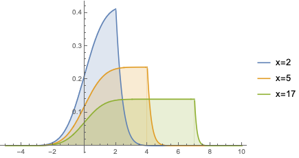
(a)

(b)

(c)

(d)

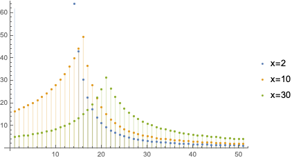
(e)

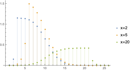
(f)

Figure 1: The functions $x^{\prime}\mapsto\mathcal{L}_{p,x^{\prime}}^{\ell}(\chi^{\ell}(x^{\prime},x))=K_{p}^{\ell}(x,x^{\prime})/p(x)$ for different (fixed) values of $x$ and $p$ the standard normal distribution (Figure 1(a)); Beta distribution with parameters 1.3 and 2.4 (Figure 1(b)); Gamma distribution with parameters 1.3 and 2.4 (Figure 1(c)); binomial distribution with parameters $(20,.2)$ (Figure 1(d)); Poisson distribution with parameter 15 (Figure 1(e)); hypergeometric distribution with parameters 100, 50 and 500 (Figure 1(f)).

Theorem 3.1 gives upper and lower bounds of functionals of random variables with coefficients (weights) expressed in terms of Stein operators. This result provides so-called weighted Poincaré inequalities such as those described in [64]; it also contains the main result from [45]. While the lower bound – some type of Cramer-Rao bound – has long been known to have a very simple proof via Stein operators, a proof for the upper bounds has always been either elusive or rather complicated outside of the gaussian case (see e.g. [64]). The representation formulae obtained for Stein integral operators will turn out to simplify the work considerably.

Theorem 3.1 (Klaassen bounds).

For any $c\in\mathcal{F}_{\ell}^{(1)}(p)$ we have for all $f$ such that $\bar{f}^{2}\in L^{1}(p)$:

$$\mathrm{Var}[f(X)]\geq\frac{\mathbb{E}\left[c(X)(\Delta^{-\ell}f(X))\right]^{2}}{\mathbb{E}\left[\big{(}\mathcal{T}_{p}^{\ell}c(X)\big{)}^{2}\right]}$$ (3.15)

with equality if and only if there exist $\alpha,\beta$ real numbers such that $f(x)=\alpha\mathcal{T}_{p}^{\ell}c(x)+\beta$ for all $x\in\mathcal{S}(p)$. Moreover, if $h\in L^{1}(p)$ is decreasing then for all $f$ such that $\mathcal{L}_{p}^{\ell}h(\cdot)f(\cdot-\ell)\in\mathcal{F}^{(1)}_{\ell}(p)$ we have

$$\mathrm{Var}[f(X)]\leq\mathbb{E}\left[(\Delta^{-\ell}f(X))^{2}\frac{-\mathcal{L}_{p}^{\ell}h(X)}{\Delta^{-\ell}h(X)}\right]$$ (3.16)

with equality if and only if there exist $\alpha,\beta$ real numbers such that $f(x)=\alpha h(x)+\beta$ for all $x\in\mathcal{S}(p)$.

Remark 3.2.

The requirement that $h$ be decreasing is not necessary; all that is needed is in fact that ${-\mathcal{L}_{p}^{\ell}h(X)}/{\Delta^{-\ell}h(X)}>0$ almost surely.

Proof of Theorem 3.1.

The lower bound (3.15) is an almost immediate consequence of (3.1). Indeed, using the fact that $\mathcal{T}_{p}^{\ell}c(X)\in\mathcal{F}^{(0)}(p)$ for all $c\in\mathcal{F}^{\ell}(p)$ we have

$$\mathbb{E}\left[c(X)\big{(}\Delta^{-\ell}f(X)\big{)}\right]^{2} =\mathbb{E}\left[\big{(}\mathcal{T}_{p}^{\ell}c(X)\big{)}f(X)\right]^{2}=\mathbb{E}\left[\big{(}\mathcal{T}_{p}^{\ell}c(X)\big{)}\bar{f}(X)\right]^{2}$$

$$\leq\mathbb{E}\left[\big{(}\mathcal{T}_{p}^{\ell}c(X)\big{)}^{2}\right]\mathrm{Var}[f(X)]$$

by the Cauchy-Schwarz inequality. To see (3.16) we simply apply (3.5) and the Cauchy-Schwarz inequality to obtain

$$\mathrm{Var}[f(X)]=\mathbb{E}\left[\bar{f}(X)f(X)\right]=\mathbb{E}\left[\Delta^{-\ell}f(X)\frac{K_{p}^{\ell}(X,X^{\prime})}{p(X)p(X^{\prime})}\Delta^{-\ell}f(X^{\prime})\right]$$

$$=\mathbb{E}\left[\left\{\frac{\Delta^{-\ell}f(X)}{\sqrt{\Delta^{-\ell}h(X)}}\sqrt{\frac{K_{p}^{\ell}(X,X^{\prime})}{p(X)p(X^{\prime})}\Delta^{-\ell}h(X^{\prime})}\right\}\left\{\frac{\Delta^{-\ell}f(X^{\prime})}{\sqrt{\Delta^{-\ell}h(X^{\prime})}}\sqrt{\frac{K_{p}^{\ell}(X,X^{\prime})}{p(X)p(X^{\prime})}\Delta^{-\ell}h(X)}\right\}\right]$$

$$\leq\mathbb{E}\left[\frac{(\Delta^{-\ell}f(X))^{2}}{\Delta^{-\ell}h(X)}\frac{K_{p}^{\ell}(X,X^{\prime})}{p(X)p(X^{\prime})}\Delta^{-\ell}h(X^{\prime})\right];$$

using (3.7) finishes the proof. ∎

Example 3.4 (Binomial bounds).

Let $X\sim\mathrm{Bin}(n,p)$. From previous developments we obtain the upper and lower bounds

$$\frac{\mathbb{E}\left[X\Delta^{-}f(X)\right]^{2}}{np}\leq\mathrm{Var}[f(X)]\leq(1-p)\mathbb{E}\left[X(\Delta^{-}f(X))^{2}\right];$$

$$\frac{\mathbb{E}\left[(X-n)\Delta^{+}f(X)\right]^{2}}{n(1-p)}\leq\mathrm{Var}[f(X)]\leq\mathbb{E}\left[p(n-X)(\Delta^{+}f(X))^{2}\right].$$

Example 3.5 (Poisson bounds).

Let $X\sim\mathrm{Pois}(\lambda)$. From previous developments we obtain the upper and lower bounds

$$\frac{\mathbb{E}\left[X\Delta^{-}f(X)\right]^{2}}{\lambda}\leq\mathrm{Var}[f(X)]\leq\mathbb{E}\left[X(\Delta^{-}f(X))^{2}\right];$$

$$\mathbb{E}\left[\Delta^{+}f(X)\right]^{2}\leq\mathrm{Var}[f(X)]\leq\lambda\mathbb{E}\left[(\Delta^{+}f(X))^{2}\right].$$

Example 3.6 (Beta bounds).

Let $X\sim\mathrm{Beta}(\alpha,\beta)$. From previous developments we obtain the upper and lower bounds

$$\frac{(\alpha+\beta)(\alpha+\beta+1)}{\alpha\beta}\mathbb{E}\left[X(1-X)f^{\prime}(X)\right]^{2}\leq\mathrm{Var}[f(X)]\leq\frac{1}{\alpha+\beta}\mathbb{E}\left[X(1-X)(f^{\prime}(X))^{2}\right]$$

4 A Lagrange formula and Papathanassiou-type variance expansions

This section begins with a third representation for the Stein operator $\mathcal{L}_{p}^{\ell}$; surprisingly, this result seems to be new.

Lemma 4.1 (Representation formula III).

Let $X,X_{1},X_{2}$ be independent copies of $X\sim p$ with support $\mathcal{S}(p)$. We define

$$\Phi^{\ell}_{p}(u,x,v)=\chi^{\ell}(u,x)\chi^{-\ell}(x,v)/p(x)$$ (4.1)

for all $u,v\in\mathcal{S}(p)$ (note that $\Phi^{\ell}_{p}(u,x,v)=0$ for $u\geq v$). Then, for all $h\in L^{1}(p)$ we have

$$-\mathcal{L}_{p}^{\ell}h(x)=\mathbb{E}\left[(h(X_{2})-h(X_{1}))\Phi^{\ell}_{p}(X_{1},x,X_{2})\right].$$ (4.2)

Proof.

First notice that, under the assumptions, $\mathbb{E}[\chi^{\ell}(X,x)+\chi^{-\ell}(x,X)]=1$ for all $x\in\mathcal{X}$. Suppose without loss of generality that $\mathbb{E}[h(X)]=0$. Using that $X_{1},X_{2}$ are i.i.d., we reap

$$\mathbb{E}\big{[}(h(X_{1})-h(X_{2}))\chi^{\ell}(X_{1},x)\chi^{-\ell}(x,X_{2})\big{]}$$

$$=\mathbb{E}\big{[}h(X_{1})\chi^{\ell}(X_{1},x)\big{]}\mathbb{E}[\chi^{-\ell}(x,X_{2})]-\mathbb{E}\big{[}h(X_{2})\chi^{-\ell}(x,X_{2})\big{]}\mathbb{E}[\chi^{\ell}(X_{1},x)]$$

$$=\mathbb{E}\big{[}h(X_{1})\chi^{\ell}(X_{1},x)\big{]}\mathbb{E}[\chi^{-\ell}(x,X_{2})]-\mathbb{E}\big{[}h(X_{2})\big{(}1-\chi^{\ell}(X_{2},x)\big{)}\big{]}\mathbb{E}[\chi^{\ell}(X_{1},x)]$$

$$=\mathbb{E}\big{[}h(X)\chi^{\ell}(X,x)\big{]}\big{(}\mathbb{E}[\chi^{-\ell}(x,X)]+\mathbb{E}[\chi^{\ell}(X,x)]\big{)}.$$

The conclusion follows after recalling (2.2). ∎

Combining (3.4) and (4.2) we easily obtain the following identities which, together, will ultimately lead to our infinite expansions for variances.

Lemma 4.2.

Let $X\sim p$ with support $\mathcal{S}(p)$. For all $x_{1},x_{2}\in\mathcal{S}(p)$, we have

$$g(x_{2})-g(x_{1})=\mathbb{E}\left[\Phi^{\ell}_{p}(x_{1},X,x_{2})\Delta^{-\ell}g(X)\right].$$ (4.3)

If $X_{1},X_{2}$ are independent copies of $X$ then

$$\mathrm{Var}[g(X)]=\mathbb{E}\left[\left(g(X_{2})-g(X_{1})\right)^{2}\mathbb{I}_{[X_{1}<X_{2}]}\right]$$ (4.4)

for all $g\in L^{2}(p)$.

Proof.

Identity (4.3) follows from the (trivial) observation that

$$\mathbb{E}\left[\frac{\chi^{\ell}(x_{1},X)\chi^{-\ell}(X,x_{2})}{p(X)}\Delta^{-\ell}g(X)\right] =\int_{\mathcal{S}(p)}\chi^{\ell}(x_{1},x)\chi^{-\ell}(x,x_{2})\Delta^{-\ell}g({{\color[rgb]{0,0,1}x}})d\mu(x)$$

which is equal to $g(x_{2})-g(x_{1})$ for all $x_{1}<x_{2}\in\mathcal{S}(p)$ and all $\ell\in\left\{-1,0,1\right\}$. Using (3.4) followed by (4.2), we get

$$\mathrm{Var}[g(X)] =\mathbb{E}[-\mathcal{L}_{p}^{\ell}g(X)\Delta^{-\ell}g(X)]$$

$$=\mathbb{E}\left[\mathbb{E}\big{[}\big{(}g(X_{2})-g(X_{1})\big{)}\Phi_{p}^{\ell}(X_{1},X,X_{2})\,|\,X\big{]}\Delta^{-\ell}g(X)\right]$$

$$=\mathbb{E}\left[\big{(}g(X_{2})-g(X_{1})\big{)}\Phi_{p}^{\ell}(X_{1},X,X_{2})\Delta^{-\ell}g(X)\right]$$

$$=\mathbb{E}\left[\big{(}g(X_{2})-g(X_{1})\big{)}\mathbb{E}\left[\Phi_{p}^{\ell}(X_{1},X,X_{2})\Delta^{-\ell}g(X)\,|\,X_{1},X_{2}\right]\mathbb{I}_{[X_{1}<X_{2}]}\right]$$

$$=\mathbb{E}\left[\big{(}g(X_{2})-g(X_{1})\big{)}^{2}\mathbb{I}_{[X_{1}<X_{2}]}\right],$$

whence the claim. ∎

Remark 4.1.

In fact, treating the discrete and continuous cases separately, one could also obtain identity (4.4) as a direct application of Lagrange’s identity (a.k.a. the Cauchy-Schwarz inequality with remainder) which reads, in the finite discrete case, as

$$\left(\sum_{k=u}^{v}a_{k}^{2}\right)\left(\sum_{k=u}^{v}b_{k}^{2}\right)-\left(\sum_{k=u}^{v}a_{k}b_{k}\right)^{2}=\sum_{i=u}^{v-1}\sum_{j=i+1}^{v}(a_{i}b_{j}-a_{j}b_{i})^{2}$$ (4.5)

with $a_{k}=g(k)\sqrt{p(k)}$ and $b_{k}=\sqrt{p(k)}$ for $k=0,\ldots,n$. Identity (4.5) and its continuous counterpart will play a crucial role in the sequel; it will be more suited to our cause under the following form.

Lemma 4.3 (A probabilistic Lagrange identity).

Let $X,X_{1},X_{2}$ be independent random variables with distribution $p$ and $a,b$ any two functions such that the expectations below exist. Then

$$\mathbb{E}\left[a(X)b(X)\Phi^{\ell}_{p}(u,X,v)\right]^{2} =\mathbb{E}\left[(a(X))^{2}\Phi^{\ell}_{p}(u,X,v)\right]\mathbb{E}\left[(b(X))^{2}\Phi^{\ell}_{p}(u,X,v)\right]$$

$$\quad-\mathbb{E}\left[(a(X_{1})b(X_{2})-a(X_{2})b(X_{1}))^{2}\Phi^{\ell}_{p}(u,X_{1},X_{2},v)\right]$$ (4.6)

where

$$\Phi^{\ell}_{p}(u,x_{1},x_{2},v)=\frac{\chi^{\ell}(u,x_{1})\chi^{\ell^{2}}(x_{1},x_{2})\chi^{-\ell}(x_{2},v)}{p(x_{1})p(x_{2})}.$$ (4.7)

Proof of Lemma 4.3.

The proof follows from expanding the second term in (4.3),

$$\mathbb{E}\left[(a(X_{1})b(X_{2})-a(X_{2})b(X_{1}))^{2}\Phi^{\ell}_{p}(u,X_{1},X_{2},v)\right]$$

$$= \mathbb{E}\left[(a(X_{1})^{2}b(X_{2})^{2}+a(X_{2})^{2}b(X_{1})^{2})\Phi^{\ell}_{p}(u,X_{1},v)\Phi^{\ell}_{p}(u,X_{2},v)\Delta^{\ell^{2}}(X_{1},X_{2})\right]$$

$$-2\mathbb{E}\left[(a(X_{1})b(X_{2})a(X_{2})b(X_{1}))\Phi^{\ell}_{p}(u,X_{1},v)\Phi^{\ell}_{p}(u,X_{2},v)\Delta^{\ell^{2}}(X_{1},X_{2})\right].$$

By symmetry,

$$\mathbb{E}\left[(a(X_{1})b(X_{2})-a(X_{2})b(X_{1}))^{2}\Phi^{\ell}_{p}(u,X_{1},X_{2},v)\right]$$

$$= \mathbb{E}\left[(a(X_{1})b(X_{2})-a(X_{2})b(X_{1}))^{2}\Phi^{\ell}_{p}(u,X_{2},X_{1},v)\right].$$

Now $\Delta^{\ell^{2}}(X_{1},X_{2})+\Delta^{\ell^{2}}(X_{2},X_{1})=1$ when $X_{1}=X_{2}$, and vanishes otherwise, and for $X_{1}=X_{2}$, it holds that $(a(X_{1})b(X_{2})-a(X_{2})b(X_{1}))^{2}=0$. Hence

$$\mathbb{E}\left[(a(X_{1})b(X_{2})-a(X_{2})b(X_{1}))^{2}\Phi^{\ell}_{p}(u,X_{1},X_{2},v)\right]$$

$$= \frac{1}{2}\mathbb{E}\left[(a(X_{1})b(X_{2})-a(X_{2})b(X_{1}))^{2}\Phi^{\ell}_{p}(u,X_{1},v)\Phi^{\ell}_{p}(u,X_{2},v)\right].$$

Exploiting the independence of $X_{1}$ and $X_{2}$ now yields the conclusion. ∎

Remark 4.2.

For ease of reference, we detail (4.7):

$$\Phi^{0}_{p}(u,x_{1},x_{2},v)=\Phi^{0}_{p}(u,x_{1},x_{2})\frac{\chi^{0}(x_{2},v)}{p(x_{2})}=\frac{\chi^{0}(u,x_{1})\chi^{0}(x_{1},x_{2})\chi^{0}(x_{2},v)}{p(x_{1})p(x_{2})}$$ (4.8)

$$\Phi^{-}_{p}(u,x_{1},x_{2},v)=\Phi^{-}_{p}(u,x_{1},x_{2})\frac{\chi^{+}(x_{2},v)}{p(x_{2})}=\frac{\chi^{-}(u,x_{1})\chi^{+}(x_{1},x_{2})\chi^{+}(x_{2},v)}{p(x_{1})p(x_{2})}$$ (4.9)

$$\Phi^{+}_{p}(u,x_{1},x_{2},v)=\frac{\chi^{+}(u,x_{1})}{p(x_{1})}\Phi^{+}_{p}(x_{1},x_{2},v)=\frac{\chi^{+}(u,x_{1})\chi^{+}(x_{1},x_{2})\chi^{-}(x_{2},v)}{p(x_{1})p(x_{2})}$$ (4.10)

Theorem 4.1.

Fix $\ell\in\left\{-1,0,1\right\}$ and define the sequence $\boldsymbol{\ell}=(\ell_{n})_{n\geq 1}$ such that $\ell_{n}=0$ for all $n$ if $\ell=0$, otherwise $\ell_{n}\in\left\{-1,1\right\}$ arbitrarily chosen. Consider a sequence $(h_{n})_{n\geq 1}$ of real valued functions $h_{i}:{\rm I\kern-1.60004ptR}\to{\rm I\kern-1.60004ptR}$ such that $\mathbb{P}[\Delta^{\ell_{i}}h_{2i-1}(X)>0]=1$ for all $i\geq 1$. Starting with some function $g$, we also recursively define the sequence $(g_{k})_{0\leq k\leq n}$ by $g_{0}(x)=g(x)$ and $g_{i}(x)={\Delta^{\ell_{i}}g_{i}(x)}/{\Delta^{\ell_{i}}h_{i}(x)}$ for all $x\in\mathcal{S}(p)$. Finally, starting from $\Phi_{1,1}^{\boldsymbol{\ell}}(x_{1},x,x_{2})=\Phi^{\ell_{1}}_{p}(x_{1},x,x_{2})$ and $\Phi_{1,2}^{\boldsymbol{\ell}}(x_{1},x_{3},x_{4},x_{2})=\Phi^{\ell_{1}}_{p}(x_{1},x_{3},x_{4},x_{2})$ we define recursively for $n\geq 2$

$$\Phi_{n,1}^{\boldsymbol{\ell}}(x_{1},x_{3},\ldots,x_{2n-1},x,x_{2n},\ldots,x_{2})$$

$$\qquad=\Phi^{\ell_{n}}_{p}(x_{2n-1},x,x_{2n})\Phi_{n-1,2}^{\boldsymbol{\ell}}(x_{1},x_{3},\ldots,x_{2n-1},x_{2n},\ldots,x_{2})$$ (4.11)

$$\Phi_{n,2}^{\boldsymbol{\ell}}(x_{1},x_{3},\ldots,x_{2n-1},x_{2n+1},x_{2n+2},x_{2n},\ldots,x_{2})$$

$$\qquad=\Phi^{\ell_{n}}_{p}(x_{2n-1},x_{2n+1},x_{2n+2},x_{2n})\Phi_{n-1,2}^{\boldsymbol{\ell}}(x_{1},x_{3},\ldots,x_{2n-1},x_{2n},\ldots,x_{2})$$ (4.12)

at any sequence $(x_{j})_{j\geq 1}$. Then, for all $g\in L^{2}(p)$ and all $n\geq 1$ we have

$$\mathrm{Var}[g(X)]= \sum_{k=1}^{n}(-1)^{k-1}\mathbb{E}\left[\frac{\left(\Delta^{-\ell_{k}}g_{k-1}(X)\right)^{2}}{\Delta^{-\ell_{k}}h_{k}(X)}\Gamma_{k}^{\boldsymbol{\ell}}(X)\right]+(-1)^{n}R_{n}^{\boldsymbol{\ell}}$$ (4.13)

where

$$\Gamma_{k}^{\boldsymbol{\ell}}(x)=\mathbb{E}\Bigg{[}(h_{k}(X_{2k})-h_{k}(X_{2k-1}))\prod_{i=1}^{k-1}\Delta^{-\ell_{i}}h_{i}(X_{2i+1},X_{2i+2})\Phi_{k,1}^{\boldsymbol{\ell}}(X_{1},\ldots,X_{2k-1},x,X_{2k},\ldots,X_{2})\Bigg{]}$$ (4.14)

and

$$R_{n}^{\boldsymbol{\ell}} =\mathbb{E}\Bigg{[}\left(g_{n}(X_{2n+2})-g_{n}(X_{2n+1})\right)^{2}\prod_{i=1}^{n}\Delta^{-\ell_{i}}h_{i}(X_{2i-1},X_{2i})\Phi_{n,2}^{\boldsymbol{\ell}}(X_{1},\ldots X_{2n+1},X_{2n+2},\ldots,X_{2})\Bigg{]}$$ (4.15)

(we introduce the notation $\Delta^{\ell}h_{k}(x,y)=\Delta^{\ell}h_{k}(x)\Delta^{\ell}h_{k}(y)$ and an empty product is set to 1).

Proof.

Throughout this proof we write $\mathbb{E}_{X_{i_{1}},\ldots,X_{i_{k}}}\left[\Psi(X_{1},\ldots,X_{n})\right]$ to denote the expectation of multivariable function $\Psi(X_{1},\ldots,X_{n})$ taken only with respect to $X_{i_{1}},\ldots,X_{i_{k}}$ (that is, conditionally on all non-mentioned variables). Starting from (4.4) and using (4.3):

$$\mathrm{Var}[g(X)] =\mathbb{E}\left[\left(g(X_{2})-g(X_{1})\right)^{2}\mathbb{I}_{[X_{1}<X_{2}]}\right]$$

$$=\mathbb{E}\left[\left(\mathbb{E}_{X}\left[\Phi^{\ell_{1}}_{p}(X_{1},X,X_{2})\Delta^{-\ell_{1}}g(X)\right]\right)^{2}\mathbb{I}_{[X_{1}<X_{2}]}\right].$$ (4.16)

Next, for any $h_{1}$ such that $\mathbb{P}[\Delta^{-\ell_{1}}h_{1}(X)>0]=1$, we have, thanks to (4.3) and conditionally on $X_{1},X_{2}$:

$$\bigg{(}\mathbb{E}_{X}\left[\Phi^{\ell_{1}}_{p}(X_{1},X,X_{2})\Delta^{-\ell_{1}}g(X)\right]\bigg{)}^{2}=\bigg{(}\mathbb{E}_{X}\left[\Phi^{\ell_{1}}_{p}(X_{1},X,X_{2})\frac{\Delta^{-\ell_{1}}g(X)}{\sqrt{\Delta^{-\ell_{1}}h_{1}(X)}}\sqrt{\Delta^{-\ell_{1}}h_{1}(X)}\right]\bigg{)}^{2}$$

$$=\mathbb{E}_{X}\left[\frac{\big{(}\Delta^{-\ell_{1}}g(X)\big{)}^{2}}{{\Delta^{-\ell_{1}}h_{1}(X)}}\Phi^{\ell_{1}}_{p}(X_{1},X,X_{2})\right]\mathbb{E}_{X^{\prime}}\left[\Delta^{-\ell_{1}}h(X^{\prime})\Phi^{\ell_{1}}_{p}(X_{1},X^{\prime},X_{2})\right]$$

$$\quad-\mathbb{E}_{X_{3},X_{4}}\left[\bigg{(}\frac{\Delta^{-\ell_{1}}g(X_{3})}{\sqrt{\Delta^{-\ell_{1}}h_{1}(X_{3})}}\sqrt{\Delta^{-\ell_{1}}h_{1}(X_{4})}-\frac{\Delta^{-\ell_{1}}g(X_{4})}{\sqrt{\Delta^{-\ell_{1}}h_{1}(X_{4})}}\sqrt{\Delta^{-\ell_{1}}h_{1}(X_{3})}\bigg{)}^{2}\Phi^{\ell_{1}}_{p}(X_{1},X_{3},X_{4},X_{2})\right]$$

$$=:I_{1}(X_{1},X_{2})-I_{2}(X_{1},X_{2})$$ (4.17)

($X^{\prime}$ in the second line is another independent copy of $X$). We need to compute $\mathbb{E}[I_{1}(X_{1},X_{2})\mathbb{I}_{[X_{1}<X_{2}]}]-\mathbb{E}[I_{2}(X_{1},X_{2})\mathbb{I}_{[X_{1}<X_{2}]}]$. We begin by noting that, in the discrete case, the strict inequality in the indicator $\mathbb{I}_{[X_{1}<X_{2}]}$ is implicit in $\Phi^{\ell_{1}}_{p}(X_{1},X,X_{2})=\chi^{\ell_{1}}(X_{1},X)\chi^{-\ell_{1}}(X,X_{2})/p(X)$ and hence a fortiori also in $\Phi^{\ell_{1}}_{p}(X_{1},X_{3},X_{4},X_{2})$. In the continuous case there is no difference between $\mathbb{I}_{[X_{1}<X_{2}]}$ and $\mathbb{I}_{[X_{1}\leq X_{2}]}$. We treat the two terms separately. First,

$$\mathbb{E}[I_{1}(X_{1},X_{2})\mathbb{I}_{[X_{1}<X_{2}]}]$$

$$=\mathbb{E}\left[\mathbb{E}_{X}\left[\frac{\big{(}\Delta^{-\ell_{1}}g(X)\big{)}^{2}}{{\Delta^{-\ell_{1}}h_{1}(X)}}\Phi^{\ell_{1}}_{p}(X_{1},X,X_{2})\right]\mathbb{E}_{X^{\prime}}\left[\Delta^{-\ell_{1}}h_{1}({X^{\prime}})\Phi^{\ell_{1}}_{p}(X_{1},{X^{\prime}},X_{2})\right]\mathbb{I}_{[X_{1}<X_{2}]}\right]$$

$$=\mathbb{E}\left[\frac{\big{(}\Delta^{-\ell_{1}}g(X)\big{)}^{2}}{{\Delta^{-\ell_{1}}h_{1}(X)}}\Phi^{\ell_{1}}_{p}(X_{1},X,X_{2})\mathbb{E}_{X^{\prime}}\left[\Delta^{-\ell_{1}}h_{1}({X^{\prime}})\Phi^{\ell_{1}}_{p}(X_{1},{X^{\prime}},X_{2})\right]\right]$$

$$=\mathbb{E}\left[\frac{\big{(}\Delta^{-\ell_{1}}g(X)\big{)}^{2}}{{\Delta^{-\ell_{1}}h_{1}(X)}}\big{(}h_{1}(X_{2})-h_{1}(X_{1})\big{)}\Phi^{\ell_{1}}_{p}(X_{1},X,X_{2})\right],$$ (4.18)

the last identity by (4.3). For the second term we have

$$\mathbb{E}[I_{2}(X_{1},X_{2})\mathbb{I}_{[X_{1}<X_{2}]}]$$

$$=\mathbb{E}\left[\bigg{(}\frac{\Delta^{-\ell_{1}}g(X_{3})}{\sqrt{\Delta^{-\ell_{1}}h_{1}(X_{3})}}\sqrt{\Delta^{-\ell_{1}}h_{1}(X_{4})}-\frac{\Delta^{-\ell_{1}}g(X_{4})}{\sqrt{\Delta^{-\ell_{1}}h_{1}(X_{4})}}\sqrt{\Delta^{-\ell_{1}}h_{1}(X_{3})}\bigg{)}^{2}\Phi^{\ell_{1}}_{p}(X_{1},X_{3},X_{4},X_{2})\right]$$

$$=\mathbb{E}\left[\Delta^{-\ell_{1}}h_{1}(X_{3})\Delta^{-\ell_{1}}h_{1}(X_{4})\big{(}g_{1}(X_{4})-g_{1}(X_{3})\big{)}^{2}\Phi^{\ell_{1}}_{p}(X_{1},X_{3},X_{4},X_{2})\right]$$ (4.19)

with $g_{1}(x)={\Delta^{-\ell_{1}}g(x)}/{\Delta^{-\ell_{1}}h_{1}(x)}$, as anticipated. Combining (4.18) and (4.19) we obtain (4.13) at $n=1$.

To pursue towards $n=2$, starting from (4.19), we simply apply the same process as above:

$$\mathbb{E}\left[\Delta^{-\ell_{1}}h_{1}(X_{3},X_{4})\left(g_{1}(X_{4})-g_{1}(X_{3})\right)^{2}\Phi^{\boldsymbol{\ell}}_{1,2}(X_{1},X_{3},X_{4},X_{2})\right]$$

$$=\mathbb{E}\left[\Delta^{-\ell_{1}}h_{1}(X_{3},X_{4})\left(\mathbb{E}_{X}\left[\Phi^{\ell_{2}}_{p}(X_{3},X,X_{4})\Delta^{-\ell_{2}}g_{1}(X)\right]\right)^{2}\Phi^{\boldsymbol{\ell}}_{1,2}(X_{1},X_{3},X_{4},X_{2})\right]$$

$$=:\mathbb{E}\left[\Delta^{-\ell_{1}}h_{1}(X_{3},X_{4})I_{21}(X_{3},X_{4})\Phi^{\boldsymbol{\ell}}_{1,2}(X_{1},X_{3},X_{4},X_{2})\right]$$

$$\quad-\mathbb{E}\left[\Delta^{-\ell_{1}}h_{1}(X_{3},X_{4})I_{22}(X_{3},X_{4})\Phi^{\boldsymbol{\ell}}_{1,2}(X_{1},X_{3},X_{4},X_{2})\right]$$

with $I_{2j},j=1,2$ defined (in terms of a function $h_{2}$) through (4.17). Again we treat the terms separately:

$$\mathbb{E}\left[\Delta^{-\ell_{1}}h_{1}(X_{3},X_{4})I_{21}(X_{3},X_{4})\Phi^{\boldsymbol{\ell}}_{1,2}(X_{1},X_{3},X_{4},X_{2})\right]$$

$$=\mathbb{E}\left[\frac{(\Delta^{-\ell_{2}}g_{1}(X))^{2}}{\Delta^{-\ell_{2}}h_{2}(X)}\big{(}h_{2}(X_{4})-h_{2}(X_{3})\big{)}\Delta^{-\ell_{1}}h_{1}(X_{3},X_{4})\Phi^{\ell_{2}}_{p}(X_{3},X,X_{4})\Phi^{\boldsymbol{\ell}}_{1,2}(X_{1},X_{3},X_{4},X_{2})\right]$$

and

$$\mathbb{E}\left[\Delta^{-\ell_{1}}h_{1}(X_{3},X_{4})I_{22}(X_{3},X_{4})\Phi^{\boldsymbol{\ell}}_{1,2}(X_{1},X_{3},X_{4},X_{2})\right]$$

$$=\mathbb{E}\left[\Delta^{-\ell_{1}}h_{1}(X_{3},X_{4})\Delta^{-\ell_{2}}h_{2}(X_{5},X_{6})\big{(}g_{2}(X_{6})-g_{2}(X_{5})\big{)}^{2}\Phi^{\ell_{2}}_{p}(X_{3},X_{5},X_{6},X_{4})\Phi^{\boldsymbol{\ell}}_{1,2}(X_{1},X_{3},X_{4},X_{2})\right].$$

The complete statement follows by induction and careful bookkeeping of all the indices. ∎

Remark 4.3 (About the assumptions in the theorem).

A stronger sufficient condition on the functions $h_{i}$ is that they be strictly increasing throughout $\mathcal{S}(p)$, in which case the condition $\Delta^{\ell}h(x)>0$ is guaranteed. The prototypical example of such a sequence is $h_{i}(x)=x$ for all $i\geq 1$ which clearly satisfies all the required assumptions. When $\ell\neq 0$ then the condition that $\mathbb{P}[\Delta^{\ell_{k}}h_{k}(X)>0]=1$ is in fact too restrictive because, as has been made clear in the proof, the recurrence only implies that $\Delta^{\ell_{k}}h_{k}(x)$ needs to be positive on $(a+i(k),b-j(k))$ for some indices $i(k),j(k)$ depending on the behavior of $X_{2k-1}$ and $X_{2k}$ (see the line just below equation (4.16) when $k=1$). In particular the sequence necessarily stops if $\mathcal{S}(p)$ is bounded, since after a certain number of iterations the indicator functions defining $\Phi_{n,j}^{\boldsymbol{\ell}}$ will be 0 everywhere.

Remark 4.4.

When $g$ is a $d$th-degree polynomial, we obtain an exact expansion of the variance in (4.13) with respect to the $\Gamma_{k}^{\boldsymbol{\ell}}(x)$ functions ($k=1,\ldots,d$) as the $R_{n}^{\boldsymbol{\ell}}$ is defined in terms of the $n$-th derivative of $g$.

The functions $\Gamma_{k}^{\ell_{k}}$ defined in (4.14) are some sort of generalization of Peccati’s and Ledoux’ gamma mentioned in the Introduction. To see this, choose $h_{k}(x)=x$ for all $k$ (arguably the most natural choice) for which $\Delta^{\ell}h_{k}(x)=1\mbox{ for all }k$ so that

$$\Gamma_{k}^{\boldsymbol{\ell}}(x) =\mathbb{E}\left[(X_{2k}-X_{2k-1})\Phi_{k,1}^{\boldsymbol{\ell}}(X_{1},\ldots,X_{2k-1},x,X_{2k},\ldots,X_{2})\right]$$ (4.20)

for all $k\geq 1$ we have. Expliciting the above leads to the expressions:

$$\Gamma_{1}^{\ell_{1}}(x)=\mathbb{E}\bigg{[}(X_{2}-X_{1})\frac{\chi^{\ell_{1}}(X_{1},x)\chi^{-\ell_{1}}(x,X_{2})}{p(x)}\bigg{]}$$

$$\Gamma_{2}^{\ell_{1},\ell_{2}}(x)=\mathbb{E}\bigg{[}(X_{4}-X_{3})\frac{\chi^{\ell_{1}}(X_{1},X_{3})\chi^{\ell_{2}}(X_{3},x)\chi^{-\ell_{2}}(x,X_{4})\chi^{-\ell_{1}}(X_{4},X_{2})}{p(X_{3})p(x)p(X_{4})}\bigg{]}$$

$$\Gamma_{3}^{\ell_{1},\ell_{2},\ell_{3}}(x)=\mathbb{E}\bigg{[}(X_{6}-X_{5})\frac{\chi^{\ell_{1}}(X_{1},X_{3})\chi^{\ell_{2}}(X_{3},X_{5})\chi^{\ell_{3}}(X_{5},x)\chi^{-\ell_{3}}(x,X_{6})\chi^{-\ell_{2}}(X_{4},X_{2})\chi^{-\ell_{1}}(X_{4},X_{2})}{p(X_{3})p(X_{5})p(x)p(X_{6})p(X_{4})}\bigg{]}$$

$$\mathrm{etc.}$$

In particular $\Gamma_{1}^{\boldsymbol{\ell}}(x)=\tau_{p}^{\ell_{1}}(x)$ is the Stein kernel of $X$. The next lemma follows by induction.

Lemma 4.4.

If $\ell=0$ then

$$\Gamma_{k}^{0}(x)=\frac{1}{p(x)}\mathbb{E}\Bigg{[}\frac{1}{k!(k-1)!}(x-X_{1})^{k-1}(X_{2}-x)^{k-1}(X_{{2}}-X_{1})\mathbb{I}_{[X_{1}\leq x\leq X_{2}]}\Bigg{]}.$$ (4.21)

and if ${\boldsymbol{\ell}}\in\{-1,1\}^{k}$, then

$$\Gamma_{k}^{\boldsymbol{\ell}}(x)=\frac{1}{p(x)}\mathbb{E}\Bigg{[}\frac{1}{k!(k-1)!}(x-X_{1}-a_{\boldsymbol{\ell}}+1)^{\lceil k-1\rceil}(X_{2}-x-b_{\boldsymbol{\ell}}+1)^{\lceil k-1\rceil}(X_{{2}}-X_{1})\mathbb{I}_{[X_{1}+a_{\boldsymbol{\ell}}\leq x\leq X_{2}+b_{\boldsymbol{\ell}}]}\Bigg{]}.$$ (4.22)

where $a^{\lceil k\rceil}(x)=a(a+1)\cdots(a+k-1)$, $a_{\boldsymbol{\ell}}=\sum_{i=1}^{k}\frac{l_{i}(l_{i}+1)}{2}$ and $b_{\boldsymbol{\ell}}=\sum_{i=1}^{k}\frac{l_{i}(1-l_{i})}{2}$.

Proof.

We define $\gamma_{k}^{\boldsymbol{\ell}}(x,X_{1},X_{2})$ such that

$$\Gamma_{k}^{\boldsymbol{\ell}}(x)=\frac{1}{p(x)}\mathbb{E}\bigg{[}\gamma_{k}^{\boldsymbol{\ell}}(x,X_{1},X_{2})\bigg{]}$$ (4.23)

The proof is complete if we have, in the continuous case,

$$\gamma_{k}^{0}(x)=\frac{1}{k!(k-1)!}(x-X_{1})^{k-1}(X_{2}-x)^{k-1}(X_{{2}}-X_{1})\mathbb{I}_{[X_{1}\leq x\leq X_{2}]}$$ (4.24)

and in the discrete case,

$$\gamma_{k}^{\boldsymbol{\ell}}(x)=\frac{1}{k!(k-1)!}(x-X_{1}-A_{\boldsymbol{\ell}}+1)^{\lceil k-1\rceil}(X_{2}-x-B_{\boldsymbol{\ell}}+1)^{\lceil k-1\rceil}(X_{{2}}-X_{1})\mathbb{I}_{[X_{1}+A_{\boldsymbol{\ell}}\leq x\leq X_{2}+B_{\boldsymbol{\ell}}]}$$ (4.25)

We prove (4.24) and (4.25) by induction. Firstly, for $k=1$, $\ell=0,1$ or -1, we obtain

$$\Gamma^{\ell}_{1}(x) =\frac{1}{p(x)}\mathbb{E}\Bigg{[}(X_{{2}}-X_{1})\mathbb{I}_{[X_{1}+\frac{\ell(\ell+1)}{2}\leq x\leq X_{2}+\frac{\ell(1-\ell)}{2}]}\Bigg{]}$$

After conditioning with respect to the “extreme” variables, the expression of (4.20) can be rewritten as

$$\Gamma_{k+1}^{\boldsymbol{\ell}}(x)= \mathbb{E}\left[(X_{2k+2}-X_{2k+1})\Phi_{k+1,1}^{\boldsymbol{\ell}}(X_{1},\ldots,X_{2k+1},x,X_{2k+2},\ldots,X_{2})\right]$$

$$= \mathbb{E}\bigg{[}(X_{2k+2}-X_{2k+1})\prod_{i=1}^{k}\left(\frac{\chi^{\ell_{i}}(X_{2i-1},X_{2i+1})}{p(X_{2i+1})}\frac{\chi^{-\ell_{i}}(X_{2i+2},X_{2i})}{p(X_{2i+2})}\right)\frac{\chi^{\ell_{k+1}}(X_{2k+1},x)\chi^{-\ell_{k+1}}(x,X_{2k+2})}{p(x)}\bigg{]}$$

$$=: \frac{1}{p(x)}\mathbb{E}_{X_{1},X_{2}}\bigg{[}\mathbb{E}_{X_{3},X_{4}}\bigg{[}\frac{\chi^{\ell_{1}}(X_{1},X_{3})}{p(X_{3}}\frac{\chi^{-\ell_{1}}(X_{4},X_{2})}{p(X_{4}}\gamma_{k}^{\ell_{2},\ldots,\ell_{k+1}}(x,X_{3},X_{4})\,\Bigg{|}\,X_{1},X_{2}\bigg{]}\bigg{]}$$ (4.26)

This expression allows us to conclude the assertion by induction, in the continuous case and in the discrete case separately. ∎

Remark 4.5.

The results e.g. from [60, 43, 4, 5, 1] permit to identify that if $X\sim p$ is Pearson distributed then $\Gamma_{k}^{0}(x)=\tau_{p}(x)^{k}$, and if $X$ is Ord distributed then $\Gamma_{k}^{0}(x)=\tau_{p}(x)^{[k]}$ with $f^{[k]}(x)=f(x-k+1)\cdots f(x)$.

Example 4.1 (Normal bounds).

Direct computations show that if $X\sim\mathcal{N}(0,1)$ then $\Gamma_{1}^{0}(x)=1$ and $\Gamma_{2}^{0}(x)=\frac{1}{2}$ so that the first two bounds become

$$\mathrm{Var}[g(X)] =\mathbb{E}\left[g^{\prime}(X)^{2}\right]-R_{1}$$

$$=\mathbb{E}\left[g^{\prime}(X)^{2}\right]-\frac{1}{2}\mathbb{E}\left[g^{\prime\prime}(X)^{2}\right]+R_{2}$$

Example 4.2 (Beta bounds).

Direct computations show that if $X\sim\mathrm{Beta}(\alpha,\beta)$ then $\Gamma_{1}^{0}(x)=x(1-x)/(\alpha+\beta)$ and $\Gamma_{2}^{0}(x)=(x(1-x))^{2}/(2(\alpha+\beta)(\alpha+\beta+1))$ so that the first two bounds become

$$\mathrm{Var}[g(X)] =\frac{1}{\alpha+\beta}\mathbb{E}\left[X(1-X)g^{\prime}(X)^{2}\right]-R_{1}$$

$$=\frac{1}{\alpha+\beta}\mathbb{E}\left[X(1-X)g^{\prime}(X)^{2}\right]-\frac{1}{2(\alpha+\beta)(\alpha+\beta+1)}\mathbb{E}\left[{X^{2}(1-X)^{2}}g^{\prime\prime}(X)^{2}\right]+R_{2}$$

Example 4.3 (Gamma bounds).

Direct computations show that $X\sim\mathrm{Gamma}(\alpha,\beta)$ then $\Gamma_{1}^{0}(x)=\beta x$ and $\Gamma_{2}^{0}(x)=\frac{1}{2}\beta^{2}x^{2}$ so that the first two bounds become

$$\mathrm{Var}[g(X)] =\beta\mathbb{E}\left[Xg^{\prime}(X)^{2}\right]-R_{1}$$

$$=\beta\mathbb{E}\left[Xg^{\prime}(X)^{2}\right]-\frac{\beta^{2}}{2}\mathbb{E}\left[X^{2}g^{\prime\prime}(X)^{2}\right]+R_{2}$$

Example 4.4 (Laplace bounds).

Direct computations show that $X\sim\mathrm{Laplace}(0,1)$ then $\Gamma_{1}^{0}(x)=1+|x|$ and $\Gamma_{2}^{0}(x)=\frac{1}{2}x^{2}+|x|+1$ so that the first two bounds become

$$\mathrm{Var}[g(X)] ={\mathbb{E}\left[(1+|X|)g^{\prime}(X)^{2}\right]-R_{1}}$$

$$=\mathbb{E}\left[(1+|X|)g^{\prime}(X)^{2}\right]-\mathbb{E}\left[(1+|X|+X^{2}/2)g^{\prime\prime}(X)^{2}\right]+R_{2}$$

In the discrete case, there is much more flexibility in the construction of the bounds as any permutation of $+1$ and $-1$ is allowed at every stage (that is, for every $k$), leading to:

$$\mathrm{Var}[g(X)] =\mathbb{E}\left[\Gamma_{1}^{+}(X)(\Delta^{-}g(X))^{2}\right]-R_{1}^{+}=\mathbb{E}\left[\Gamma_{1}^{-}(X)(\Delta^{+}g(X))^{2}\right]-R_{1}^{-}$$

and at order 2:

$$\mathrm{Var}[g(X)] =\mathbb{E}\left[\Gamma_{1}^{+}(X)(\Delta^{-}g(X))^{2}\right]-\mathbb{E}\left[\Gamma_{2}^{++}(X)(\Delta^{-,-}g(X))^{2}\right]+R_{2}^{++}$$

$$=\mathbb{E}\left[\Gamma_{1}^{+}(X)(\Delta^{-}g(X))^{2}\right]-\mathbb{E}\left[\Gamma_{2}^{+-}(X)(\Delta^{-,+}g(X))^{2}\right]+R_{2}^{+-}$$

$$=\mathbb{E}\left[\Gamma_{1}^{-}(X)(\Delta^{+}g(X))^{2}\right]-\mathbb{E}\left[\Gamma_{2}^{-+}(X)(\Delta^{+,-}g(X))^{2}\right]+R_{2}^{-+}$$

$$=\mathbb{E}\left[\Gamma_{1}^{-}(X)(\Delta^{+}g(X))^{2}\right]-\mathbb{E}\left[\Gamma_{2}^{--}(X)(\Delta^{+,+}g(X))^{2}\right]+R_{2}^{--}.$$

where we use the concise notation $\Delta^{\ell_{1},\ell_{2}}g(X)$ for $\Delta^{\ell_{2}}\left(\Delta^{\ell_{1}}g(X)\right)$.

We detail the bounds in several settings.

Example 4.5 (Binomial bounds).

Direct computations show that $X\sim\mathrm{Bin}(n,p)$ then

$$\Gamma_{1}^{+}(x)=(1-p)x,\quad\Gamma_{1}^{-}(x)=p(n-x)$$

and

$$\Gamma_{2}^{++}(x)=\frac{1}{2}(1-p)^{2}x(x-1),\quad\Gamma_{2}^{+-}(x)=\Gamma_{2}^{-+}(x)=\frac{1}{2}p(1-p)x(n-x)\mbox{ and }\Gamma_{2}^{--}(x)=\frac{1}{2}p^{2}(n-x-1)(n-x)$$

so that the first bounds become at order 1:

$$\mathrm{Var}[g(X)] =(1-p)\mathbb{E}\left[X(\Delta^{-}g(X))^{2}\right]-R_{1}^{+}$$

$$=p\mathbb{E}\left[(n-X)(\Delta^{+}g(X))^{2}\right]-R_{1}^{-}$$

and at order 2:

$$\mathrm{Var}[g(X)] =(1-p)\mathbb{E}\left[X(\Delta^{-}g(X))^{2}\right]-\frac{1}{2}(1-p)^{2}\mathbb{E}\left[X(X-1)(\Delta^{-,-}g(X))^{2}\right]+R_{2}^{++}$$

$$=(1-p)\mathbb{E}\left[X(\Delta^{-}g(X))^{2}\right]-\frac{1}{2}p(1-p)\mathbb{E}\left[X(n-X)(\Delta^{-,+}g(X))^{2}\right]+R_{2}^{+-}$$

$$=p\mathbb{E}\left[(n-X)(\Delta^{+}g(X))^{2}\right]-\frac{1}{2}p(1-p)\mathbb{E}\left[X(n-X)(\Delta^{+,-}g(X))^{2}\right]+R_{2}^{-+}$$

$$=p\mathbb{E}\left[(n-X)(\Delta^{+}g(X))^{2}\right]-\frac{1}{2}p^{2}\mathbb{E}\left[(n-X-1)(n-X)(\Delta^{+,+}g(X))^{2}\right]+R_{2}^{--}$$

We note that [38, Theorem 1.3] prove the bound

$$\mbox{Var}[g(X)]\leq\mathbb{E}\left[\left(\frac{X}{n}\Delta^{-}g(X)+\frac{n-X}{n}\Delta^{+}g(X)\right)^{2}\right]$$

which is very close to a combination of the above (see their Remark 3.3) but, as far as we can see, remains a different result. The similarity of the two results is striking but seemingly fortuitous.

Example 4.6 (Poisson bounds).

Direct computations show that if $X\sim\mathrm{Pois}(\lambda)$ then

$$\Gamma_{1}^{+}(x)=x,\quad\Gamma_{1}^{-}(x)=\lambda$$

and

$$\Gamma_{2}^{++}(x)=\frac{1}{2}x(x-1),\quad\Gamma_{2}^{+-}(x)=\Gamma_{2}^{-+}(x)=\frac{1}{2}\lambda x\mbox{ and }\Gamma_{2}^{--}(x)=\frac{1}{2}\lambda^{2}$$

so that the first bounds become at order 1:

$$\mathrm{Var}[g(X)] =\mathbb{E}\left[X(\Delta^{-}g(X))^{2}\right]-R_{1}^{+}$$

$$=\lambda\mathbb{E}\left[(\Delta^{+}g(X))^{2}\right]-R_{1}^{-}$$

and at order 2:

$$\mathrm{Var}[g(X)] =\mathbb{E}\left[X(\Delta^{-}g(X))^{2}\right]-\frac{1}{2}\mathbb{E}\left[X(X-1)(\Delta^{-,-}g(X))^{2}\right]+R_{2}^{++}$$

$$=\mathbb{E}\left[X(\Delta^{-}g(X))^{2}\right]-\frac{1}{2}\lambda\mathbb{E}\left[X(\Delta^{-,+}g(X))^{2}\right]+R_{2}^{+-}$$

$$=\lambda\mathbb{E}\left[(\Delta^{+}g(X))^{2}\right]-\frac{1}{2}\lambda\mathbb{E}\left[X(\Delta^{+,-}g(X))^{2}\right]+R_{2}^{-+}$$

$$=\lambda\mathbb{E}\left[(\Delta^{+}g(X))^{2}\right]-\frac{1}{2}\lambda^{2}\mathbb{E}\left[(\Delta^{+,+}g(X))^{2}\right]+R_{2}^{--}$$

5 Olkin-Shepp-type bounds

As mentioned in the introduction, a matrix extension of Chernoff’s gaussian bound (1.16) is due to [59], and the result is obtained by expanding the test functions in the Hermite basis. An extension of this result to a wide class of multivariate densities is proposed in [2] (see also references therein). Once again, our notations allow to extend this result to arbitrary densities of real-valued random variables.

Theorem 5.1 (Olkin-Shepp first order bound).

Let all previous notations and assumptions prevail. Then, for all $h$ such that $\Delta^{-\ell}h(X)\neq 0$ a.s.

$$\begin{pmatrix}\mathrm{Var}[f(X)]&\mathrm{Cov}[f(X),g(X)]\\ \mathrm{Cov}[f(X),g(X)]&\mathrm{Var}[g(X)]\end{pmatrix}\leq\mathbb{E}\left[\begin{pmatrix}\big{(}\Delta^{-\ell}f(X)\big{)}^{2}&\Delta^{-\ell}f(X)\Delta^{-\ell}g(X)\\ \Delta^{-\ell}f(X)\Delta^{-\ell}g(X)&\big{(}\Delta^{-\ell}g(X)\big{)}^{2}\end{pmatrix}\frac{\Gamma_{1}^{\ell}(X)}{\Delta^{-\ell}h(X)}\right]$$

with

$$\Gamma_{1}^{\ell}(x)=\mathbb{E}\left[(h(X_{2})-h(X_{1}))\Phi_{p}^{\ell}(X_{1},x,X_{2})\right],$$

as defined in (4.14).

Remark 5.1.

Taking determinants in Theorem 5.1 gives the variance-covariance inequality

$$\mathrm{Var}[f(X)]\mathrm{Var}[g(X)]-\{\mathrm{Cov}[f(X),g(X)]\}^{2}$$

$$\leq\mathbb{E}\left[\big{(}\Delta^{-\ell}f(X)\big{)}^{2}\frac{\Gamma_{1}^{\ell}(X)}{\Delta^{-\ell}h(X)}\right]\mathbb{E}\left[\big{(}\Delta^{-\ell}g(X)\big{)}^{2}\frac{\Gamma_{1}^{\ell}(X)}{\Delta^{-\ell}h(X)}\right]-\mathbb{E}\left[\Delta^{-\ell}f(X)\Delta^{-\ell}g(X)\frac{\Gamma_{1}^{\ell}(X)}{\Delta^{-\ell}h(X)}\right]^{2}.$$ (5.1)

This observation was made in [59] for the special case of $p$ being the normal distribution $\mathcal{N}(\mu,\sigma^{2})$ and $h(x)=x$, for which $\Delta^{-\ell}$ is the usual derivative and $\Gamma_{1}^{\ell}(x)=\sigma^{2}$.

Remark 5.2.

Multiplying the result in Theorem 5.1 by the vector $(1,0)^{\prime}$ gives the variance inequality

$$\mathrm{Var}[f(X)]\leq\mathbb{E}\left[\big{(}\Delta^{-\ell}f(X)\big{)}^{2}\frac{\Gamma_{1}^{\ell}(X)}{\Delta^{-\ell}h(X)}\right]$$ (5.2)

which corresponds to the first order of Theorem 4.1.

The proof of Theorem 5.1 relies on a lemma which seems natural but for which we have not found a reference, and therefore we include one for completeness.

Lemma 5.1 (Matrix Cauchy-Schwarz inequality).

Let $\mathbf{v}(x)=(a(x),b(x))^{\prime}\in{\rm I\kern-1.60004ptR}^{2}$ and $f:{\rm I\kern-1.60004ptR}\to{\rm I\kern-1.60004ptR}$ any function. Then

$$\mathbb{E}\left[\mathbf{v}(X)f(X)\Phi_{p}{{}^{\ell}}(u,X,v)\right]\mathbb{E}\left[\mathbf{v}(X)^{\prime}f(X)\Phi_{p}{{}^{\ell}}(u,X,v)\right]$$

$$\qquad\qquad\leq\mathbb{E}\left[\mathbf{v}(X)\mathbf{v}(X)^{\prime}\Phi_{p}{{}^{\ell}}(u,X,v)\right]\mathbb{E}\left[f(X)^{2}\Phi_{p}{{}^{\ell}}(u,X,v)\right],$$ (5.3)

where inequality in the above is in the Loewner ordering, i.e. the difference is nonnegative definite.

Remark 5.3.

In light of the proof of (5.3), there is no doubt that a similar matrix version of the Lagrange identity (4.3) holds as well. We have not explored this any further, but in particular higher order upper bound as in [2] should be within reach.

Proof of Lemma 5.1.

In the proof we use the shorthand $h$ instead of $h(X)$, $h_{i}$ instead of $h(X_{i})$, $\Phi_{p}$ or $\Phi_{p}^{i}$ for $\Phi{{}_{p}^{\ell}}(u,X{{}_{i}},v)$ and $\Phi_{p}^{ij}=\Phi{{}_{p}^{\ell}}(u,X_{i},X_{j},v)$. Writing (5.3) out in coordinates, it is necessary to prove that

$$R:=\begin{pmatrix}\mathbb{E}\left[a^{2}\Phi_{p}\right]\mathbb{E}\left[f^{2}\Phi_{p}\right]-\mathbb{E}\left[af\Phi_{p}\right]^{2}&\mathbb{E}[ab\Phi_{p}]\mathbb{E}\left[f^{2}\Phi_{p}\right]-\mathbb{E}\left[af\Phi_{p}\right]\mathbb{E}\left[{b}f\Phi_{p}\right]\\ \mathbb{E}[ab\Phi_{p}]\mathbb{E}\left[f^{2}\Phi_{p}\right]-\mathbb{E}\left[af\Phi_{p}\right]\mathbb{E}\left[{b}f\Phi_{p}\right]&\mathbb{E}\left[b^{2}\Phi_{p}\right]\mathbb{E}\left[f^{2}\Phi_{p}\right]-\mathbb{E}\left[bf\Phi_{p}\right]^{2}\end{pmatrix}$$

is nonnegative definite. Next we apply (4.3) to each component of the matrix $R$, which leads to

$$R=\begin{pmatrix}\mathbb{E}\left[(a_{3}f_{4}-a_{4}f_{3})^{2}\Phi_{p}^{34}\right]&\mathbb{E}\left[(a_{3}f_{4}-a_{4}f_{3})(b_{3}f_{4}-b_{4}f_{3})\Phi_{p}^{34}\right]\\ \mathbb{E}\left[(a_{3}f_{4}-a_{4}f_{3})(b_{3}f_{4}-b_{4}f_{3})\Phi_{p}^{34}\right]&\mathbb{E}\left[(b_{3}f_{4}-b_{4}f_{3})^{2}\Phi_{p}^{34}\right]\end{pmatrix}.$$

Clearly the diagonal terms are already of the correct form. For the off-diagonal terms we note that

$$\mathbb{E}[(a_{3}f_{4}-a_{4}f_{3})(b_{3}f_{4}-b_{4}f_{3})\Phi_{p}^{34}]$$

$$=\mathbb{E}[a_{3}f_{4}b_{3}f_{4}\Phi_{p}^{34}]-\mathbb{E}[a_{3}f_{4}b_{4}f_{3}\Phi_{p}^{34}]-\mathbb{E}[a_{4}f_{3}b_{3}f_{4}\Phi_{p}^{34}]+\mathbb{E}[a_{4}f_{3}b_{4}f_{3}\Phi_{p}^{34}]$$

so that, using

$$\Phi_{p}^{34}=\Phi_{p}(u,X_{3},X_{4},v)=\Phi_{p}(u,X_{3},v)\Phi_{p}(u,X_{4},v)\mathbb{I}[X_{3}<X_{4}],$$

we get

$$\mathbb{E}[(a_{3}f_{4}-a_{4}f_{3})(b_{3}f_{4}-b_{4}f_{3})\Phi_{p}^{34}]$$

$$=\mathbb{E}\left[a_{3}b_{3}\Phi_{p}^{3}f_{4}^{2}\Phi_{p}^{4}\mathbb{I}[X_{3}<X_{4}]\right]-\mathbb{E}\left[a_{3}f_{3}\Phi_{p}^{3}b_{4}f_{4}\Phi_{p}^{4}\mathbb{I}[X_{3}<X_{4}]\right]$$

$$\quad-\mathbb{E}\left[b_{3}f_{3}\Phi_{p}^{3}a_{4}f_{4}\Phi_{p}^{4}\mathbb{I}[X_{3}<X_{4}]\right]+\mathbb{E}\left[f_{3}^{2}\Phi_{p}^{3}a_{4}b_{4}\Phi_{p}^{4}\mathbb{I}[X_{3}<X_{4}]\right]$$

$$=\mathbb{E}\left[a_{3}b_{3}\Phi_{p}^{3}f_{4}^{2}\Phi_{p}^{4}\mathbb{I}[X_{3}<X_{4}]\right]-\mathbb{E}\left[a_{3}f_{3}\Phi_{p}^{3}b_{4}f_{4}\Phi_{p}^{4}\mathbb{I}[X_{3}<X_{4}]\right]$$

$$\quad-\mathbb{E}\left[b_{4}f_{4}\Phi_{p}^{4}a_{3}f_{3}\Phi_{p}^{3}\mathbb{I}[X_{4}\leq X_{3}]\right]+\mathbb{E}\left[f_{4}^{2}\Phi_{p}^{4}a_{3}b_{3}\Phi_{p}^{3}\mathbb{I}[X_{4}<X_{3}]\right]$$

$$=\mathbb{E}\left[a_{3}b_{3}\Phi_{p}^{3}f_{4}^{2}\Phi_{p}^{4}(\mathbb{I}[X_{3}<X_{4}]+\mathbb{I}[X_{4}<X_{3}])\right]-\mathbb{E}\left[b_{4}f_{4}\Phi_{p}^{4}a_{3}f_{3}\Phi_{p}^{3}(\mathbb{I}[X_{3}<X_{4}]+\mathbb{I}[X_{4}<X_{3}])\right]$$

which leads to

$$R=\mathbb{E}\left[\begin{pmatrix}a_{3}f_{4}-a_{4}f_{3}\\ b_{3}f_{4}-b_{4}f_{3}\end{pmatrix}\begin{pmatrix}a_{3}f_{4}-a_{4}f_{3}&b_{3}f_{4}-b_{4}f_{3}\end{pmatrix}\Phi_{p}^{34}\right]$$ (5.4)

and the claim follows. ∎

Proof of Theorem 5.1.

The variances can be expressed using (4.4) and, using successively (3.4), (4.2) and (4.3), the covariance matrix can be rewritten by

$$\begin{pmatrix}\mathrm{Var}[f(X)]&\mathrm{Cov}[f(X),g(X)]\\ \mathrm{Cov}[f(X),g(X)]&\mathrm{Var}[g(X)]\end{pmatrix}$$

$$=\mathbb{E}\left[\begin{pmatrix}f(X_{2})-f(X_{1})\\ g(X_{2})-g(X_{1})\end{pmatrix}\begin{pmatrix}f(X_{2})-f(X_{1})&g(X_{2})-g(X_{1})\end{pmatrix}\mathbb{I}_{X_{1}<X_{2}}\right].$$ (5.5)

Using, as usual, the representation

$$f(X_{2})-f(X_{1})=\mathbb{E}\left[\frac{\Delta^{-\ell}f(X_{3})}{\sqrt{\Delta^{-\ell}h(X_{3})}}\sqrt{\Delta^{-\ell}h(X_{3})}\Phi_{P}^{\ell}(X_{1},X_{3},X_{2})|X_{1},X_{2}\right]$$ (5.6)

the claim follows by applying the Matrix Cauchy-Schwarz inequality (5.3) to the vector $\mathbf{v}(x)=\begin{pmatrix}\frac{\Delta^{-\ell}f(x)}{\sqrt{\Delta^{-\ell}h(x)}}&\frac{\Delta^{-\ell}g(x)}{\sqrt{\Delta^{-\ell}h(x)}}\end{pmatrix}^{\prime}$ and the function $f(x)=\sqrt{\Delta^{-\ell}h(x)}$. ∎

Example 5.1 (Normal bounds).

Direct application of (5.1) show that, by taking $h(x)=x$, if $X\sim\mathcal{N}(0,1)$ then

$$\mathrm{Var}[f(X)]\mathrm{Var}[g(X)]-\{\mathrm{Cov}[f(X),g(X)]\}^{2} \leq\mathbb{E}\left[\big{(}f^{\prime}(X)\big{)}^{2}\right]\mathbb{E}\left[\big{(}g^{\prime}(X)\big{)}^{2}\right]-\mathbb{E}\left[f^{\prime}(X)g^{\prime}(X)\right]^{2}$$

A direct application of (5.2) gives us the first order upper bound

$$\mbox{Var}[g(X)]\leq\mathbb{E}[g^{\prime}(X)^{2}].$$

which was already obtained in (1.16) and in Example 4.1.

Example 5.2 (Poisson bounds).

Direct application of (5.1) show that, by taking $h(x)=x$, if $X\sim\mathrm{Pois}(\lambda)$ then $\mathrm{Var}[f(X)]\mathrm{Var}[g(X)]-\{\mathrm{Cov}[f(X),g(X)]\}^{2}$ is bounded by

$$\mathbb{E}\left[\big{(}\Delta^{-}f(X)\big{)}^{2}X\right]\mathbb{E}\left[\big{(}\Delta^{-}g(X)\big{)}^{2}X\right]-\mathbb{E}\left[\Delta^{-}f(X)\Delta^{-}g(X)X\right]^{2}$$

and by

$$\lambda^{2}\mathbb{E}\left[\big{(}\Delta^{+}f(X)\big{)}^{2}\right]\mathbb{E}\left[\big{(}\Delta^{+}g(X)\big{)}^{2}\right]-\lambda^{2}\mathbb{E}\left[\Delta^{+}f(X)\Delta^{+}g(X)\right]^{2}.$$

Moreover, by (5.2), we find two first order upper bounds from Example 3.5:

$$\mbox{Var}[g(X)]\leq\mathbb{E}[X\big{(}\Delta^{-}g(X)\big{)}^{2}]\mbox{ and }\mbox{Var}[g(X)]\leq\lambda\mathbb{E}[\big{(}\Delta^{+}g(X)\big{)}^{2}].$$

6 Applications of the representations to estimating Stein factors

Recall that if $\mathcal{A}_{p}$ is as in (2.6) from Definition 2.4 and $\mathcal{H}$ is a collection of $h:{\rm I\kern-1.60004ptR}\to{\rm I\kern-1.60004ptR}$ belonging to $L^{1}(p)$, the “$\mathcal{A}_{p}$ Stein equation on $\mathcal{H}$” is the functional equation

$$\mathcal{A}_{p}g(x)=h(x)-\mathbb{E}[h(X)],\quad x\in\mathcal{S}(p)$$ (6.1)

whose solutions are

$$g(x)=\frac{\mathcal{L}_{p}^{\ell}h(x)}{\mathcal{L}_{p}^{\ell}\eta(x)}$$ (6.2)

with the convention that $g(x)=0$ for all $x$ outside of $\mathcal{S}(p)$. Uniform in $\mathcal{H}$ bounds on $g$ and its derivatives are known as Stein factors; in practice it is useful to have information on $\|g_{h}\|,\|\Delta^{\ell}g_{h}\|$ also for some specific functions $h$ (particularly $h(x)=x$). We conclude the paper with an application of Lemma 4.1 towards understanding properties of solutions (6.2). The result is immediate from previous developments.

Proposition 6.1.

1. If $h$ is monotone then $\mathcal{L}_{p}^{\ell}h(x)$ does not change sign.

2. If, for all $h\in\mathcal{H}$, there exists a monotone function $\eta$ such that $|h(x)-h(y)|\leq k|\eta(x)-\eta(y)|$ for all $x,y$ then the function $g$ defined in (6.2) satisfies $|g(x)|\leq k$. In particular if $\mathcal{H}$ is the collection of Lipschitz functions with constant $1$ then $\|g\|_{\infty}\leq 1$.

3. Let $P$ and $\bar{P}=1-P$ be the cdf and survival function of $p$, respectively, and define the function

   $$R^{\ell}(x)=\frac{P(x-\ell(\ell+1)/2)\bar{P}(x+\ell(\ell-1)/2)}{p(x)}$$ (6.3)

   for all $x\in\mathcal{S}(p)$. We always have

   $$\left|\mathcal{L}_{p}^{\ell}h(x)\right|\leq 2\|h\|_{\infty}\frac{\mathbb{E}[\chi^{\ell}(X_{1},x)]\mathbb{E}[\chi^{-\ell}(x,X_{2})]}{p(x)}=2\|h\|_{\infty}R^{\ell}(x)$$ (6.4)

   for all $x\in\mathcal{S}(p)$.

Proof.

Recall representation (4.2) which states that

$$-\mathcal{L}_{p}^{\ell}h(x)=\frac{1}{p(x)}\mathbb{E}\left[(h(X_{2})-h(X_{1}))\chi^{\ell}(X_{1},x)\chi^{-\ell}(x,X_{2})\right].$$

1. If $h(x)$ is monotone the $h(X_{2})-h(X_{1})$ is of constant sign conditionally on $\chi^{\ell}(X_{1},x)\chi^{-\ell}(x,X_{2})$.

2. Suppose that the function $\eta$ is strictly decreasing. By definition of $g$ we have, under the stated conditions,

   $$|g(x)| =\left|\frac{\mathbb{E}\left[(h(X_{2})-h(X_{1}))\chi^{\ell}(X_{1},x)\chi^{-\ell}(x,X_{2})\right]}{\mathbb{E}\left[(\eta(X_{2})-\eta(X_{1}))\chi^{\ell}(X_{1},x)\chi^{-\ell}(x,X_{2})\right]}\right|$$

   $$\leq\frac{\mathbb{E}\left[|h(X_{2})-h(X_{1})|\chi^{\ell}(X_{1},x)\chi^{-\ell}(x,X_{2})\right]}{\mathbb{E}\left[(\eta(X_{2})-\eta(X_{1}))\chi^{\ell}(X_{1},x)\chi^{-\ell}(x,X_{2})\right]}$$

   $$\leq k.$$

3. By definition,

   $$\big{|}\mathcal{L}_{p}^{\ell}h(x)\big{|}=\mathbb{E}\left[|h(X_{2})-h(X_{1})|\chi^{\ell}(X_{1},x)\chi^{-\ell}(x,X_{2})\right]\leq 2\|h\|_{\infty}\mathbb{E}\left[\chi^{\ell}(X_{1},x)\chi^{-\ell}(x,X_{2})\right]$$

   which leads to the conclusion.

∎

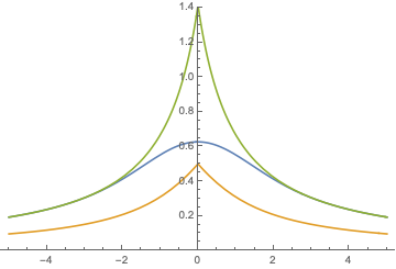
(a)

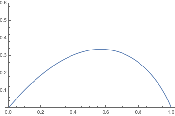
(b)

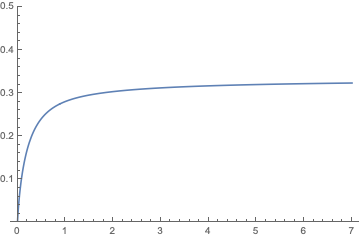
(c)

(d)

(e)

(f)

Figure 2: The functions $R^{\ell}$ for standard normal distribution (Figure 2(a), along with the upper and lower bounds from (6.5)), Beta distribution with parameters 8/9 and 1/3 (Figure 2(b)) and Gamma distribution with parameters 1/3 and 1/3 (Figure 2(c)), binomial distribution with parameters $(20,.2)$ (Figure 2(d)), Poisson distribution with parameter 15 (Figure 2(e)) and hypergeometric distribution with parameters 10, 10 and 30 (Figure 2(f)).

Example 6.1.

If $p=\phi$ is the standard Gaussian then $R(x)={\Phi(x)\big{(}1-\Phi(x)\big{)}}/{\phi(x)}$ is closely related to $r(x)$, the Mill’s ratio of the standard normal law. The study of such a function is classical and much is known. For instance, we can apply [11, Theorem 2.3] to get

$$\frac{1}{\sqrt{x^{2}+4}+x}\leq\frac{1}{2}r(x)\leq R(x)\leq r(x)\leq\frac{4}{\sqrt{x^{2}+8}+3x}$$ (6.5)

for all $x\geq 0$. Moreover, obviously, $R(x)\leq R(0)=1/2\sqrt{\pi/2}\approx 0.626$. If $h$ is bounded then $\|\mathcal{L}_{p}^{\ell}h\|_{\infty}\leq\sqrt{\pi/2}$ as is well known, see e.g. [57, Theorem 3.3.1]

References

- [1] G. Afendras, N. Balakrishnan, and N. Papadatos. Orthogonal polynomials in the cumulative Ord family and its application to variance bounds. Statistics, 52(2):364–392, 2018.
- [2] G. Afendras and N. Papadatos. On matrix variance inequalities. Journal of Statistical Planning and Inference, 141(11):3628–3631, 2011.
- [3] G. Afendras and N. Papadatos. Strengthened Chernoff-type variance bounds. Bernoulli, 20(1):245–264, 2014.
- [4] G. Afendras, N. Papadatos, and V. Papathanasiou. The discrete Mohr and Noll inequality with applications to variance bounds. Sankhyā, 69(2):162–189, 2007.
- [5] G. Afendras, N. Papadatos, and V. Papathanasiou. An extended Stein-type covariance identity for the Pearson family with applications to lower variance bounds. Bernoulli, 17(2):507–529, 2011.
- [6] B. Arras and C. Houdré. On Stein’s method for infinitely divisible laws with finite first moment. arXiv preprint arXiv:1712.10051, 2017.
- [7] B. Arras and C. Houdré. On Stein’s method for multivariate self-decomposable laws with finite first moment. arXiv preprint arXiv:1809.02050, 2018.
- [8] B. Arras and Y. Swan. IT formulae for gamma target: mutual information and relative entropy. IEEE Transactions on Information Theory, 64(2):1083–1091, 2018.
- [9] A. D. Barbour and L. H. Y. Chen. An introduction to Stein’s method, volume 4 of Lect. Notes Ser. Inst. Math. Sci. Natl. Univ. Singap. Singapore University Press, Singapore, 2005.
- [10] A. D. Barbour and L. H. Y. Chen. Stein’s method and applications, volume 5 of Lect. Notes Ser. Inst. Math. Sci. Natl. Univ. Singap. Singapore University Press, Singapore, 2005.
- [11] Á. Baricz. Mills’ ratio: monotonicity patterns and functional inequalities. Journal of Mathematical Analysis and Applications, 340(2):1362–1370, 2008.
- [12] H. J. Brascamp and E. H. Lieb. On extensions of the Brunn-Minkowski and Prékopa-Leindler theorems, including inequalities for log concave functions, and with an application to the diffusion equation. Journal of Functional Analysis, 22(4):366–389, 1976.
- [13] T. Cacoullos. On upper and lower bounds for the variance of a function of a random variable. The Annals of Probability, 10(3):799–809, 1982.
- [14] T. Cacoullos and V. Papathanasiou. On upper and lower bounds for the variance of functions of a random variable. Statist. Probab. Lett., 3:175–184, 1985.
- [15] T. Cacoullos and V. Papathanasiou. Bounds for the variance of functions of random variables by orthogonal polynomials and Bhattacharyya bounds. Statistics & Probability Letters, 4(1):21–23, 1986.
- [16] T. Cacoullos and V. Papathanasiou. Characterizations of distributions by variance bounds. Statist. Probab. Lett., 7(5):351–356, 1989.
- [17] T. Cacoullos and V. Papathanasiou. A generalization of covariance identity and related characterizations. Math. Methods Statist., 4(1):106–113, 1995.
- [18] L. H. Chen. An inequality for the multivariate normal distribution. Journal of Multivariate Analysis, 12(2):306–315, 1982.
- [19] L. H. Chen. Poincaré-type inequalities via stochastic integrals. Zeitschrift für Wahrscheinlichkeitstheorie und Verwandte Gebiete, 69(2):251–277, 1985.
- [20] L. H. Y. Chen. Poisson approximation for dependent trials. The Annals of Probability, 3(3):534–545, 1975.
- [21] L. H. Y. Chen, L. Goldstein, and Q.-M. Shao. Normal approximation by Stein’s method. Probability and its Applications (New York). Springer, Heidelberg, 2011.
- [22] H. Chernoff. A note on an inequality involving the normal distribution. The Annals of Probability, 9(3):533–535, 1981.
- [23] K. Chwialkowski, H. Strathmann, and A. Gretton. A kernel test of goodness of fit. In International Conference on Machine Learning, pages 2606–2615, 2016.
- [24] T. A. Courtade, M. Fathi, and A. Pananjady. Existence of Stein kernels under a spectral gap, and discrepancy bound. arXiv preprint arXiv:1703.07707, 2017.
- [25] P. Diaconis and S. Zabell. Closed form summation for classical distributions: variations on a theme of de Moivre. Statist. Sci., 6(3):284–302, 1991.
- [26] C. Döbler. Stein’s method of exchangeable pairs for the beta distribution and generalizations. Electronic Journal of Probability, 20(109):1–34, 2015.
- [27] W. Ehm. Binomial approximation to the Poisson binomial distribution. Statistics & Probability Letters, 11(1):7–16, 1991.
- [28] M. Ernst and Y. Swan. Stein based goodness-of-fit tests. In preparation, 2018.
- [29] X. Fang, Q.-M. Shao, and L. Xu. Multivariate approximations in wasserstein distance by stein’s method and bismut’s formula. Probability Theory and Related Fields, pages 1–35, 2018.
- [30] M. Fathi. Higher-order stein kernels for gaussian approximation. arXiv preprint arXiv:1812.02703, 2018.
- [31] M. Fathi. Stein kernels and moment maps. arXiv preprint arXiv:1804.04699, 2018.
- [32] R. E. Gaunt, A. Pickett, and G. Reinert. Chi-square approximation by Stein’s method with application to Pearson’s statistic. Annals of Applied Probability, to appear, 2016.
- [33] L. Goldstein and G. Reinert. Stein’s method and the zero bias transformation with application to simple random sampling. The Annals of Applied Probability, 7(4):935–952, 1997.
- [34] L. Goldstein and G. Reinert. Stein’s method for the Beta distribution and the Pólya-Eggenberger urn. Journal of Applied Probability, 50(4):1187–1205, 2013.
- [35] J. Gorham, A. B. Duncan, S. J. Vollmer, and L. Mackey. Measuring sample quality with diffusions. arXiv preprint arXiv:1611.06972, 2016.
- [36] J. Gorham and L. Mackey. Measuring sample quality with Stein’s method. In Advances in Neural Information Processing Systems, pages 226–234, 2015.
- [37] J. Gorham and L. Mackey. Measuring sample quality with kernels. arXiv preprint arXiv:1703.01717, 2017.
- [38] E. Hillion, O. Johnson, and Y. Yu. A natural derivative on [0, n] and a binomial Poincaré inequality. ESAIM: Probability and Statistics, 18:703–712, 2014.
- [39] C. Houdré and A. Kagan. Variance inequalities for functions of Gaussian variables. Journal of Theoretical Probability, 8(1):23–30, 1995.
- [40] C. Houdré and V. Pérez-Abreu. Covariance identities and inequalities for functionals on Wiener and Poisson spaces. The Annals of Probability, 23(1):400–419, 1995.
- [41] C. Houdré, V. Pérez-Abreu, and D. Surgailis. Interpolation, correlation identities, and inequalities for infinitely divisible variables. Journal of Fourier Analysis and Applications, 4(6):651–668, 1998.
- [42] R. W. Johnson. A note on variance bounds for a function of a Pearson variate. Statistics & Risk Modeling, 11(3):273–278, 1993.
- [43] R. W. Johnson. A note on variance bounds for a function of a Pearson variate. Statist. Decisions, 11(3):273–278, 1993.
- [44] S. Karlin. A general class of variance inequalities. Multivariate Analysis: Future Directions, Elsevier Science Publishers, New York, pages 279–294, 1993.
- [45] C. A. J. Klaassen. On an inequality of Chernoff. The Annals of Probability, 13(3):966–974, 1985.
- [46] R. Korwar. On characterizations of distributions by mean absolute deviation and variance bounds. Annals of the Institute of Statistical Mathematics, 43(2):287–295, 1991.
- [47] M. Ledoux. L’algèbre de Lie des gradients itérés d’un générateur markovien—développements de moyennes et entropies. Ann. Sci. École Norm. Sup., 28(4):435–460, 1995.
- [48] M. Ledoux, I. Nourdin, and G. Peccati. Stein’s method, logarithmic Sobolev and transport inequalities. Geometric and Functional Analysis, 25(1):256–306, 2015.
- [49] C. Ley, G. Reinert, and Y. Swan. Distances between nested densities and a measure of the impact of the prior in bayesian statistics. Annals of Applied Probability, 27(1):216–241, 2017.
- [50] C. Ley, G. Reinert, and Y. Swan. Stein’s method for comparison of univariate distributions. Probability Surveys, 14:1–52, 2017.
- [51] C. Ley and Y. Swan. Stein’s density approach and information inequalities. Electronic Communications in Probability, 18(7):1–14, 2013.
- [52] C. Ley and Y. Swan. Parametric Stein operators and variance bounds. Brazilian Journal of Probability and Statistics, 30:171–195, 2016.
- [53] Q. Liu, J. Lee, and M. Jordan. A kernelized Stein discrepancy for goodness-of-fit tests. In International Conference on Machine Learning, pages 276–284, 2016.
- [54] H. M. Luk. Stein’s method for the gamma distribution and related statistical applications. PhD thesis, University of Southern California, 1994.
- [55] L. Mackey, J. Gorham, et al. Multivariate Stein factors for a class of strongly log-concave distributions. Electronic Communications in Probability, 21, 2016.
- [56] G. Mijoule. Optimal stein factors for continuous univariate distributions. In preparation.
- [57] I. Nourdin and G. Peccati. Normal approximations with Malliavin calculus : from Stein’s method to universality. Cambridge Tracts in Mathematics. Cambridge University Press, 2012.
- [58] I. Nourdin, G. Peccati, and Y. Swan. Entropy and the fourth moment phenomenon. Journal of Functional Analysis, 266:3170–3207, 2014.
- [59] I. Olkin and L. Shepp. A matrix variance inequality. Journal of Statistical Planning and Inference, 130(1-2):351–358, 2005.
- [60] V. Papathanasiou. Variance bounds by a generalization of the Cauchy-Schwarz inequality. Statistics & probability letters, 7(1):29–33, 1988.
- [61] V. Papathanasiou. A characterization of the Pearson system of distributions and the associated orthogonal polynomials. Annals of the Institute of Statistical Mathematics, 47(1):171–176, 1995.
- [62] G. Reinert. Three general approaches to Stein’s method. In An introduction to Stein’s method, volume 4. Lecture Notes Series, Institute for Mathematical Sciences, National University of Singapore, 2004.
- [63] G. Reinert, G. Mijoule, and Y. Swan. Stein gradients and divergences for multivariate continuous distributions. arXiv:1806.03478, 2018.
- [64] A. Saumard. Weighted Poincaré inequalities, concentration inequalities and tail bounds related to the behavior of the Stein kernel in dimension one. arXiv preprint arXiv:1804.03926, 2018.
- [65] A. Saumard and J. A. Wellner. On the Isoperimetric constant, covariance inequalities and -Poincaré inequalities in dimension one. arXiv preprint arXiv:1711.00668, 2017.
- [66] A. Saumard and J. A. Wellner. Efron’s monotonicity property for measures on R2. Journal of Multivariate Analysis, 166:212–224, 2018.
- [67] C. Stein. A bound for the error in the normal approximation to the distribution of a sum of dependent random variables. In Proceedings of the Sixth Berkeley Symposium on Mathematical Statistics and Probability (Univ. California, Berkeley, Calif., 1970/1971), Vol. II: Probability theory, pages 583–602, Berkeley, Calif., 1972. Univ. California Press.
- [68] C. Stein. Approximate computation of expectations. Institute of Mathematical Statistics Lecture Notes—Monograph Series, 7. Institute of Mathematical Statistics, Hayward, CA, 1986.
- [69] C. Stein, P. Diaconis, S. Holmes, and G. Reinert. Use of exchangeable pairs in the analysis of simulations. In P. Diaconis and S. Holmes, editors, Stein’s method: expository lectures and applications, volume 46 of IMS Lecture Notes Monogr. Ser, pages 1–26. Beachwood, Ohio, USA: Institute of Mathematical Statistics, 2004.
- [70] N. Upadhye, V. Cekanavicius, and P. Vellaisamy. On Stein operators for discrete approximations. Bernoulli, 23(4A):2828–2859, 2017.