A representation of the transmutation kernels for the Schrödinger operator in terms of eigenfunctions and applications

Abstract

The representations of the kernels of the transmutation operator and of its inverse relating the one-dimensional Schrödinger operator with the second derivative are obtained in terms of the eigenfunctions of a corresponding Sturm-Liouville problem. Since both series converge slowly and in general only in a certain distributional sense we find a way to improve these expansions and make them convergent uniformly and absolutely by adding and subtracting corresponding terms. A numerical illustration of the obtained results is given.

1 Introduction

Since the first work by J. Delsarte [5], [6] the transmutation operator relating the one-dimensional Schrödinger operator $L:=\frac{d^{2}}{dx^{2}}-q(x)$ to a more elementary operator $B:=\frac{d^{2}}{dx^{2}}$ has been subject of study in hundreeds of publications devoted to spectral theory and inverse problems (see, e.g., [2], [4], [7], [14], [15], [16]). Recently in [9], [8], [13] several representations of the integral kernel of the transmutation operator in terms of series expansions in classical orthogonal polynomials have been obtained equipped with convenient recurrent formulas for the expansion coefficients. Every such representation leads to a new functional series representation of the solutions of the Schrödinger equation which enjoys a remarkable uniformness property. It admits a spectral parameter independent estimate for the approximation of the solution by partial sums of the series, which in practice allows one to compute huge numbers of eigenvalues and eigenfunctions with a controllable accuracy [9], [8], [13]. Similar results were obtained for perturbed Bessel equations [12], [10].

Up to now no similar representation has been obtained for the integral kernel of the inverse transmutation operator which is required in numerous applications, especially when solving initial-boundary value problems for PDEs with variable coefficients. Moreover, an apparently unanswered question is to find an eigenfunction expansion of both the direct and the inverse transmutation kernels, resembling the well known expansion of the Green function. Such eigenfunction series expansions additionally to their profound theoretical value acquire also computational significance due to the availability of the representations of solutions admitting the spectral parameter independent estimates and allowing one to compute huge amounts of eigendata.

In the present work we obtain an eigenfunction expansion of the integral transmutation kernels of both the direct and the inverse transmutation operators. Quite naturally, since the transmutation operators are related to pairs of differential operators, the corresponding eigenfunction expansions contain the eigendata of both differential operators.

The series expansions of both the direct and the inverse transmutation operators converge slowly and in general only in a certain distributional sense. We find the way to improve these expansions and make them convergent uniformly and absolutely by adding and subtracting corresponding terms. We give a numerical illustration of the obtained results.

2 Preliminaries

Let $q$ be a real valued function belonging to $L_{2}(0,\pi)$ and $h$, $H$ be two real numbers. Consider the Sturm-Liouville problem

$$-y^{\prime\prime}+q(x)y=\lambda y,$$ (1)

$$y^{\prime}(0)-hy(0)=y^{\prime}(\pi)+Hy(\pi)=0.$$ (2)

It defines two sequences of real numbers, the eigenvalues $\left\{\lambda_{n}\right\}_{n=0}^{\infty}$ and the weight numbers (or normalizing constants) $\left\{\alpha_{n}\right\}_{n=0}^{\infty}$ such that $\lambda_{n}\neq\lambda_{m}$ for $n\neq m$, $\alpha_{n}>0$,

$$\rho_{n}:=\sqrt{\lambda_{n}}=n+\frac{\omega}{\pi n}+\frac{k_{n}}{n},\qquad\alpha_{n}=\frac{\pi}{2}+\frac{K_{n}}{n},\qquad\left\{k_{n}\right\}_{n=0}^{\infty},\left\{K_{n}\right\}_{n=0}^{\infty}\in l_{2}.$$ (3)

The weight numbers are defined as follows $\alpha_{n}:=\int_{0}^{\pi}c^{2}(\rho_{n},x)dx$ where $c(\rho,x)$ denotes the solution of the Cauchy problem

$$-c^{\prime\prime}(\rho,x)+q(x)c(\rho,x)=\rho^{2}c(\rho,x),$$

$$c(\rho,0)=1,\qquad c^{\prime}(\rho,0)=h.$$

The value of the number $\omega$ in (3) is given by the formula

$$\omega=h+H+\frac{1}{2}\int_{0}^{\pi}q(t)\,dt.$$ (4)

Consider the Gel’fand-Levitan equation

$$G(x,t)+F(x,t)+\int_{0}^{x}F(t,s)G(x,s)\,ds=0,\qquad 0\leq t<x,$$ (5)

where $F(x,t)$ has the form

$$F(x,t)=\sum_{n=0}^{\infty}\left(\frac{\cos\rho_{n}x\cos\rho_{n}t}{\alpha_{n}}-\frac{\cos nx\cos nt}{\alpha_{n}^{0}}\right)$$ (6)

with

$$\alpha_{n}^{0}=\begin{cases}\pi/2,&n>0,\\ \pi,&n=0\end{cases}$$

and $G(x,t)$ is the kernel of a transmutation operator

$$T[u](x):=u(x)+\int_{0}^{x}G(x,s)u(s)\,ds$$ (7)

relating the operator $L:=\frac{d^{2}}{dx^{2}}-q(x)$ with the operator $B:=\frac{d^{2}}{dx^{2}}$ as follows. Let $u\in C^{2}[0,\pi]$ and $u^{\prime}(0)=0$. Then $LTu=TBu$. Denote $v:=Tu$. Then $v^{\prime}(0)-hv(0)=0$. In particular,

$$T[\cos\rho x]=c(\rho,x).$$ (8)

Let $H(x,t)$ denote the kernel of the inverse transmutation operator. That is

$$T^{-1}\left[u\right]\left(x\right)=u\left(x\right)+\int_{0}^{x}H(x,s)u(s)\,ds.$$ (9)

Recall that the kernel $H(x,t)$ can be obtained from the equality [16, Lemma 1.3.9],

$$H(x,t)-F(x,t)-\int_{0}^{t}F(x,s)G(t,s)\,ds=0,\quad 0\leq t<x.$$ (10)

The integral kernels $G$ and $H$ are continuous functions in $0\leq t\leq x\leq\pi$ and satisfy the equalities

$$G(x,x)=-H(x,x)=h+\frac{1}{2}\int_{0}^{x}q(t)\,dt.$$ (11)

3 Series representations for the transmutation kernels

Remark 1

Equations (5) and (10) can be written in the form

$$G(x,t)=-T_{x}[F](x,t)$$ (12)

and

$$H(x,t)=T_{t}[F](x,t),$$ (13)

respectively. That is, the kernels $G(x,t)$ and $H(x,t)$ are images of the function $\mp F(x,t)$ under the action of the transmutation operator applied with respect to the variable $x$ and $t$, respectively.

Theorem 2

The kernels $G(x,t)$ and $H(x,t)$ admit the following representations

$$G(x,t)=\sum_{n=0}^{\infty}\left(\frac{c\left(n,x\right)\cos nt}{\alpha_{n}^{0}}-\frac{c\left(\rho_{n},x\right)\cos\rho_{n}t}{\alpha_{n}}\right)$$ (14)

and

$$H(x,t)=\sum_{n=0}^{\infty}\left(\frac{\cos\rho_{n}x\,c\left(\rho_{n},t\right)}{\alpha_{n}}-\frac{\cos nx\,c\left(n,t\right)}{\alpha_{n}^{0}}\right),$$ (15)

where the series converge in the following distributional sense. Let the integral kernels $G(x,t)$ and $H(x,t)$ be extended by zero for $t>x$. Then for any $f\in AC\left[0,\pi\right]$ the following limit (corresponding to (14) and (15)) exists uniformly with respect to $x$,

$$\begin{split}\lim_{N\rightarrow\infty}\int_{0}^{\pi}f(t)I_{N}(x,t)dt&=\int_{0}^{\pi}f(t)\bigl{(}G(x,t)-H(t,x)\bigr{)}\,dt\\ &=-\int_{0}^{\pi}f(t)\left(F(x,t)+\int_{0}^{x}G(x,s)F(s,t)\,ds\right)dt,\end{split}$$ (16)

where

$$I_{N}(x,t)=\sum_{n=0}^{N}\left(\frac{c\left(n,x\right)\cos nt}{\alpha_{n}^{0}}-\frac{c\left(\rho_{n},x\right)\cos\rho_{n}t}{\alpha_{n}}\right).$$

Note that for $x\neq t$ only one of the values $G(x,t)$ or $H(t,x)$ can be different from zero.

Remark 3

As can be concluded from results of Section 4 and Jordan’s theorem [1, Chap.1, §39], the series in (14) and (15) converge pointwise on $[0,\pi]\times[0,\pi]$, uniformly on any compact subset of $[0,\pi)\times[0,\pi)$ and their sums are continuous functions except a jump discontinuity at $x=t=\pi$, the size of the jump being $\omega$, where $\omega$ is the parameter from (4).

Proof. Consider

$$T_{x}\left[\frac{\cos\rho_{n}x\cos\rho_{n}t}{\alpha_{n}}-\frac{\cos nx\cos nt}{\alpha_{n}^{0}}\right]=\frac{c\left(\rho_{n},x\right)\cos\rho_{n}t}{\alpha_{n}}-\frac{c\left(n,x\right)\cos nt}{\alpha_{n}^{0}}.$$

Hence, formally,

$$G(x,t)=-T_{x}\sum_{n=0}^{\infty}\left(\frac{\cos\rho_{n}x\cos\rho_{n}t}{\alpha_{n}}-\frac{\cos nx\cos nt}{\alpha_{n}^{0}}\right)=\sum_{n=0}^{\infty}\left(\frac{c\left(n,x\right)\cos nt}{\alpha_{n}^{0}}-\frac{c\left(\rho_{n},x\right)\cos\rho_{n}t}{\alpha_{n}}\right),$$

and similarly for $H$.

Due to (7), (9) and (8) one has

$$c(n,x)=\cos nx+\int_{0}^{x}G(x,s)\cos ns\,ds,\qquad\cos\rho_{n}x=c(\rho_{n},x)+\int_{0}^{x}H(x,s)c(\rho_{n},s)\,ds,$$

hence

$$\begin{split}I_{N}(x,t):&=\sum_{n=0}^{N}\left(\frac{c(n,x)\cos nt}{\alpha_{n}^{0}}-\frac{c(\rho_{n},x)\cos\rho_{n}t}{\alpha_{n}}\right)\\ &=\sum_{n=0}^{N}\left(\frac{\cos nx\cos nt}{\alpha_{n}^{0}}-\frac{\cos\rho_{n}x\cos\rho_{n}t}{\alpha_{n}}\right)\\ &\quad+\sum_{n=0}^{N}\frac{\cos nt}{\alpha_{n}^{0}}\int_{0}^{x}G(x,s)\cos ns\,ds-\sum_{n=0}^{N}\frac{\cos\rho_{n}t}{\alpha_{n}}\int_{0}^{x}H(x,s)\cos\rho_{n}s\,ds\\ &=:\Phi_{N}(x,t)+I_{N,2}(x,t)+I_{N,4}(x,t)\end{split}$$

(here we follow notation from the proof of Theorem 1.3.1 [16]).

According to [16, proof of Theorem 1.3.1] for any $f\in AC\left[0,\pi\right]$ the following limit exists

$$\lim_{N\rightarrow\infty}\max_{0\leq x\leq\pi}\int_{0}^{\pi}f(t)\Phi_{N}(x,t)\,dt=0.$$

Moreover, uniformly with respect to $x\in[0,\pi]$,

$$\lim_{N\rightarrow\infty}\int_{0}^{\pi}f(t)I_{N,2}(x,t)dt =\int_{0}^{x}f(t)G(x,t)dt,$$

$$\lim_{N\rightarrow\infty}\int_{0}^{\pi}f(t)I_{N,4}(x,t)dt =-\int_{x}^{\pi}f(t)H(t,x)dt.$$

Hence, extending $G(x,t)$ and $H(x,t)$ by zero for $x<t$ we obtain that

$$\lim_{N\rightarrow\infty}I_{N}(x,t)=\int_{0}^{\pi}f(t)\bigl{(}G(x,t)-H(t,x)\bigr{)}dt,$$

thus establishing (16).   

Remark 4

Our prime interest consists in application of the representation (15) for computing the preimages of functions under the action of the transmutation operator. From Theorem 2 we have that for any $f\in AC\left[0,\pi\right]$ the sequence

$$f(x)+\sum_{n=0}^{N}\left(\frac{\cos\rho_{n}x\,}{\alpha_{n}}\int_{0}^{x}c(\rho_{n},t)f(t)\,dt-\frac{\cos nx\,}{\alpha_{n}^{0}}\int_{0}^{x}c(n,t)f(t)\,dt\right)\\ =f(x)+\int_{0}^{x}\sum_{n=0}^{N}\left(\frac{\cos\rho_{n}x\,c(\rho_{n},t)}{\alpha_{n}}-\frac{\cos nx\,c(n,t)}{\alpha_{n}^{0}}\right)f(t)\,dt$$ (17)

tends to $T^{-1}\left[f\right]\left(x\right)$ uniformly. This gives us a practical way for computing the preimages of absolutely continuous functions reducing such computation to a number of definite integrals from (17).

Remark 5

The convergence rate of the series in the representations (6), (14) and (15) improves when the parameter $\omega$ in (3) equals zero, see Section 4 for details. Note that by appropriate choice of the constant $H$ in (2) the parameter $\omega$ can always be set to zero. Since the kernels $G(x,t)$ and $H(x,t)$ do not depend on $H$, a right choice of the constant $H$ can lead to a faster convergence of the series in (6), (14) and (15). In the next section we show how the series (14) and (15) can be modified in order to improve the convergence rate even when $\omega\neq 0$.

4 A Fourier series of a discontinuous function and improvement of convergence

Both series (14) and (15) converge rather slowly, and, moreover, for $x=t=\pi$ they converge to the exact values $G(\pi,\pi)$ and $H(\pi,\pi)$ if only the number $\omega$ from (4) equals zero.

A simple explanation (and an idea how to improve the convergence for an arbitrary value of $\omega$) can be seen in the proof of Lemma 1.3.4 from [16]. We briefly repeat the formulas for the function $F$ and later present the proof for the functions $G$ and $H$. Following [16] let us introduce the following function

$$a(x)=\sum_{n=0}^{\infty}\left(\frac{\cos\rho_{n}x}{\alpha_{n}}-\frac{\cos nx}{\alpha_{n}^{0}}\right).$$

The function $F$ can be expressed in the terms of the function $a$ as follows:

$$F(x,t)=\frac{1}{2}\bigl{(}a(x+t)+a(x-t)\bigr{)}.$$ (18)

Note that the function $F$ should be defined on the region $(x,t)\in[0,\pi]\times[0,\pi]$ to be able to consider equation (5), hence the function $a$ should be defined for $x\in[-\pi,2\pi]$.

The function $a(x)$ can be represented as (see the proof of Lemma 1.3.4 [16] and notice that the factor $1/\alpha_{n}^{0}=2/\pi$ is missing in the proof)

$$a(x)=-\frac{2\omega x}{\pi^{2}}\sum_{n=1}^{\infty}\frac{\sin nx}{n}+A_{2}(x),$$ (19)

where the function $A_{2}(x)$ is continuous on $[-\pi,2\pi]$. As for the first sum in (19), we have

$$-\frac{2\omega x}{\pi^{2}}\sum_{n=1}^{\infty}\frac{\sin nx}{n}=\begin{cases}-\frac{\omega|x|(\pi-|x|)}{\pi^{2}},&|x|<2\pi,\\ 0,&x=2\pi.\end{cases}$$ (20)

One can easily see that whenever $\omega\neq 0$, there is a jump discontinuity at $x=2\pi$, corresponding to $x=t=\pi$ for the function $F(x,t)$. Moreover, the series (20) converges slowly which implies the slow convergence of the series representing the function $F$. Same happens to the functions $G(x,t)$ and $H(x,t)$.

The idea to improve the convergence is to consider the following expression for the function $a(x)$:

$$a(x)=\frac{\cos\rho_{0}x}{\alpha_{0}}-\frac{1}{\pi}+\sum_{n=1}^{\infty}\left(\frac{\cos\rho_{n}x}{\alpha_{n}}-\frac{\cos nx}{\alpha_{n}^{0}}+\frac{2\omega x}{\pi^{2}}\frac{\sin nx}{n}\right)-\frac{\omega|x|(\pi-|x|)}{\pi^{2}},$$ (21)

that is, to subtract the slowly convergent series termwise and to add the closed expression for the whole infinite sum. Note that as an additional benefit of such reformulation, the series in (21) is uniformly convergent on the whole segment $[-\pi,2\pi]$, and hence the function $a$ given by (21) is continuous on $[-\pi,2\pi]$. Based on this idea the following result is obtained.

Theorem 6

The kernels $G$ and $H$ admit the following representations

$$\begin{split}G(x,t)&=\sum_{n=1}^{\infty}\left(\frac{c(n,x)\cos nt}{\alpha_{n}^{0}}-\frac{c(\rho_{n},x)\cos\rho_{n}t}{\alpha_{n}}-\frac{2\omega}{\pi^{2}n}\Bigl{(}x\sin nx\cos nt+t\sin nt\cos nx\Bigr{)}\right)\\ &\quad+\frac{c(0,x)}{\pi}-\frac{c(\rho_{0},x)\cos\rho_{0}t}{\alpha_{0}}+\frac{\omega}{\pi^{2}}\bigl{(}\pi x-x^{2}-t^{2}\bigr{)},\qquad 0\leq t\leq x\leq\pi\end{split}$$ (22)

and

$$\begin{split}H(x,t)&=\sum_{n=1}^{\infty}\left(\frac{\cos\rho_{n}x\,c(\rho_{n},t)}{\alpha_{n}}-\frac{\cos nx\,c(n,t)}{\alpha_{n}^{0}}+\frac{2\omega}{\pi^{2}n}\Bigl{(}x\sin nx\cos nt+t\sin nt\cos nx\Bigr{)}\right)\\ &\quad+\frac{\cos\rho_{0}x\,c(\rho_{0},t)}{\alpha_{0}}-\frac{c(0,t)}{\pi}-\frac{\omega}{\pi^{2}}\bigl{(}\pi x-x^{2}-t^{2}\bigr{)},\qquad 0\leq t\leq x\leq\pi\end{split}$$ (23)

where the series converge uniformly and absolutely.

Proof. Let us show that the series for $F(x,t)$ and $H(x,t)$ given by (6) and (15) differ from each other by an absolutely and uniformly convergent series of continuous functions. Consider

$$\begin{split}\Delta_{n}&=\left(\frac{\cos\rho_{n}x\,c(\rho_{n},t)}{\alpha_{n}}-\frac{\cos nx\,c(n,t)}{\alpha_{n}^{0}}\right)-\left(\frac{\cos\rho_{n}x\,\cos\rho_{n}t}{\alpha_{n}}-\frac{\cos nx\,\cos nt}{\alpha_{n}^{0}}\right)\\ &=\frac{\cos\rho_{n}x}{\alpha_{n}}\bigl{(}c(\rho_{n},t)-\cos\rho_{n}t\bigr{)}-\frac{\cos nx}{\alpha_{n}^{0}}\bigl{(}c(n,t)-\cos nt\bigr{)}.\end{split}$$

The function $c(\rho,t)$ satisfies the following asymptotic relation [16, (1.1.15)]

$$c(\rho,t)=\cos\rho t+q_{1}(t)\frac{\sin\rho t}{\rho}+\int_{0}^{t}q(s)\frac{\sin\rho(t-2s)}{2\rho}ds+O\left(\frac{1}{\rho^{2}}\right),\qquad\rho\rightarrow\infty,$$

where $q_{1}(t)=h+\frac{1}{2}\int_{0}^{t}q(s)\,ds$. Hence

$$\begin{split}\Delta_{n}&=q_{1}(t)\left(\frac{\cos\rho_{n}x\,\sin\rho_{n}t}{\alpha_{n}\rho_{n}}-\frac{\cos nx\,\sin nt}{n\alpha_{n}^{0}}\right)\\ &\quad+\int_{0}^{t}q(t)\left(\frac{\cos\rho_{n}x\,\sin\rho_{n}(t-2s)}{2\alpha_{n}\rho_{n}}-\frac{\cos nx\,\sin n(t-2s)}{2n\alpha_{n}^{0}}\right)ds+O\left(\frac{1}{n^{2}}\right),\qquad n\rightarrow\infty.\end{split}$$ (24)

We obtain for the first term that

$$\begin{split}\Delta_{n}^{1}&:=\frac{\cos\rho_{n}x\,\sin\rho_{n}t}{\alpha_{n}\rho_{n}}-\frac{\cos nx\,\sin nt}{n\alpha_{n}^{0}}\\ &=\frac{\cos\rho_{n}x\,\sin\rho_{n}t-\cos nx\,\sin nt}{\alpha_{n}\rho_{n}}+\left(\frac{1}{\alpha_{n}\rho_{n}}-\frac{1}{n\alpha_{n}^{0}}\right)\cos nx\,\sin nt\\ &=\frac{\sin\frac{(\rho_{n}-n)(x+t)}{2}\cos\frac{(\rho_{n}+n)(x+t)}{2}-\sin\frac{(\rho_{n}-n)(x-t)}{2}\cos\frac{(\rho_{n}+n)(x-t)}{2}}{\alpha_{n}\rho_{n}}-\frac{\alpha_{n}\rho_{n}-n\alpha_{n}^{0}}{n\alpha_{n}\alpha_{n}^{0}\rho_{n}}\cos nx\,\sin nt.\end{split}$$

Taking into account (3) one can see that $\rho_{n}-n=O(1/n)$ and $\alpha_{n}\rho_{n}-n\alpha_{n}^{0}=O(1)$, hence $\Delta_{n}^{1}=O(1/n^{2})$, $n\rightarrow\infty$. Similarly for the second term in (24).

Now, combining (18) with (21) we obtain that

$$\begin{split}F(x,t)&=\sum_{n=1}^{\infty}\left(\frac{\cos\rho_{n}x\,\cos\rho_{n}t}{\alpha_{n}}-\frac{\cos nx\,\cos nt}{\alpha_{n}^{0}}+\frac{\omega(x+t)}{\pi^{2}}\frac{\sin n(x+t)}{n}+\frac{\omega(x-t)}{\pi^{2}}\frac{\sin n(x-t)}{n}\right)\\ &\quad+\frac{\cos\rho_{0}x\,\cos\rho_{0}t}{\alpha_{0}}-\frac{1}{\pi}-\frac{\omega|x+t|(\pi-|x+t|)}{2\pi^{2}}-\frac{\omega|x-t|(\pi-|x-t|)}{2\pi^{2}}\\ &=\sum_{n=1}^{\infty}\left(\frac{\cos\rho_{n}x\,\cos\rho_{n}t}{\alpha_{n}}-\frac{\cos nx\,\cos nt}{\alpha_{n}^{0}}+\frac{2\omega}{\pi^{2}n}\Bigl{(}x\sin nx\,\cos nt+t\sin nt\,\cos nx\Bigr{)}\right)\\ &\quad+\frac{\cos\rho_{0}x\,\cos\rho_{0}t}{\alpha_{0}}-\frac{1}{\pi}-\frac{\omega}{\pi^{2}}\bigl{(}\pi\max\{x,t\}-x^{2}-t^{2}\bigr{)},\end{split}$$ (25)

where the series converges absolutely and uniformly and the equality holds whenever $x<\pi$ or $t<\pi$, i.e., $\min\{x,t\}<\pi$.

Since

$$H(x,t)=F(x,t)-\sum_{n=0}^{\infty}\Delta_{n},$$ (26)

where the series $\sum_{n=0}^{\infty}\Delta_{n}$ converges absolutely and uniformly, we immediately obtain (23) from (25) and (26) for all $x,t$ which satisfy $\min\{x,t\}<\pi$. Note also that the kernel $H$ is a continuous function on $0\leq t\leq x\leq\pi$, and the right hand side of (23) is also a continuous function on the same region. Hence the equality holds for $x=t=\pi$ as well.

The proof of (22) is completely similar.   

5 An explicit example

Let us consider an exactly solvable example which reveals some important features of the representations (14) and (15). Let $q\equiv 1$ and $h=0$. Then

$$c(\rho,x)=T[\cos\rho x]=\cos\mu x$$

where $\mu:=\sqrt{\rho^{2}-1}$. In particular,

$$c(0,x)=T[1]=\cosh x.$$

The integral kernel $G$ for this example is given by, see [11, Example 6] and [15, (1.2.7)]

$$G(x,t)=\begin{cases}\frac{xI_{1}(\sqrt{x^{2}-t^{2}})}{\sqrt{x^{2}-t^{2}}},&t<x,\\ \frac{x}{2},&t=x,\end{cases}$$ (27)

where $I_{1}$ is the modified Bessel function of the first kind.

Consider first the corresponding Sturm-Liouville problem with $H=0$. Then $c\left(\rho_{n},x\right)=\cos\sqrt{\rho_{n}^{2}-1}x$, $\rho_{n}=\sqrt{n^{2}+1}$, $\alpha_{n}=\alpha_{n}^{0}$. Hence (14) gives

$$\begin{split}G_{1}(x,t)&=\sum_{n=0}^{\infty}\frac{1}{\alpha_{n}^{0}}\left(\cos\sqrt{n^{2}-1}x\,\cos nt-\cos nx\,\cos\sqrt{n^{2}+1}t\right)\\ &=\frac{\cosh x-\cos t}{\pi}+\sum_{n=1}^{\infty}\frac{2}{\pi}\left(\cos\sqrt{n^{2}-1}x\,\cos nt-\cos nx\,\cos\sqrt{n^{2}+1}t\right).\end{split}$$ (28)

On the other hand choosing the constant $H$ in (2) equal to $-\pi/2$ we obtain that $\omega=0$. Let us construct the corresponding series representation for $G(x,t)$. Thus, $q\equiv 1$, $h=0$ and $H=-\pi/2$. Then $c(\rho_{n},x)=\cos\mu_{n}x$, where $\mu_{n}=\sqrt{\rho_{n}^{2}-1}$ are solutions of the characteristic equation

$$\mu\sin\mu\pi+\frac{\pi}{2}\cos\mu\pi=0$$ (29)

and $\alpha_{n}=\frac{\pi}{2}+\frac{\sin 2\mu_{n}\pi}{4\mu_{n}}$. Notice that the problem possesses one negative eigenvalue $\rho_{0}^{2}\approx-1.468$. The corresponding series representation for $G(x,t)$ takes the form

$$\begin{split}G_{2}(x,t)&=\frac{\cosh x}{\pi}-\frac{\cos\mu_{0}x\,\cos\rho_{0}t}{\alpha_{0}}\\ &\quad+\sum_{n=1}^{\infty}\left(\frac{2\cos\sqrt{n^{2}-1}x\,\cos nt}{\pi}-\frac{\cos\mu_{n}x\,\cos\rho_{n}t}{\alpha_{n}}\right).\end{split}$$ (30)

Additionally, for the case $h=H=0$ we consider the representation given by (22),

$$\begin{split}G_{3}(x,t)&=\sum_{n=1}^{\infty}\frac{2}{\pi}\left(\cos\sqrt{n^{2}-1}x\,\cos nt-\cos nx\,\cos\sqrt{n^{2}+1}t-\frac{x\sin nx\,\cos nt+t\sin nt\,\cos nx}{2n}\right)\\ &\quad+\frac{\cosh x-\cos t}{\pi}+\frac{\omega}{\pi^{2}}\bigl{(}\pi x-x^{2}-t^{2}\bigr{)}.\end{split}$$ (31)

We stress that the representations (28), (30) and (31) correspond to the same kernel $G(x,t)$.

We computed approximate integral kernels by truncating the series in (28), (30) and (31) and compared with the exact integral kernel at $x=\pi$. On Figure 1 we present the absolute value of the differences, 10 and 100 terms of the series were used. In accordance with Remark 3 the difference between partial sums of the series (28) and the exact value at $t=\pi$ remains close to $\pi/2$, while both series (30) and (31) converge uniformly and faster. All computations were realized in Matlab 2017a. Notice that opposite to (28) and (31), the approximation obtained from (30) requires $\mu_{n}$ to be computed numerically from (29). This was done by converting the function $\mu\sin\mu\pi+\frac{\pi}{2}\cos\mu\pi$ into a spline and finding its zeros with the aid of the Matlab routine fnzeros.

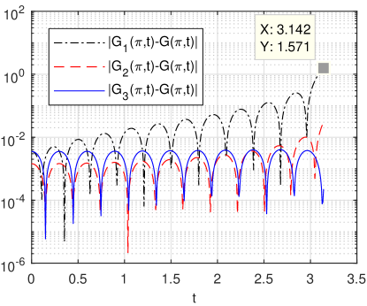
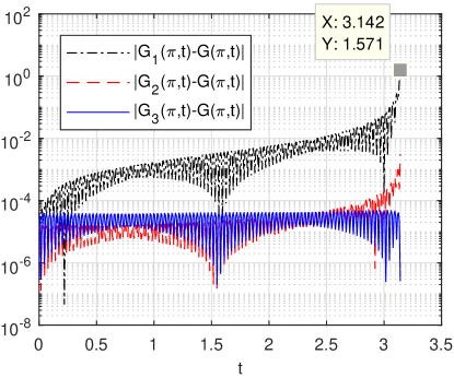
Figure 1: Absolute errors of the approximate integral kernel computed using truncated sums of the series (28), (30) and (31). Left plot: 10 terms used. Right plot: 100 terms used.

Now let us compare the convergence rate of the series applying all three representations for computing $T[1]$. Of course, in our example, $T[1]=c\left(0,x\right)=\cosh x$. Thus, using (28), (30) and (31) we construct three approximations of the function $\cosh x$,

$$\cosh x \approx 1+\frac{x\cosh x-\sin x}{\pi}+\sum_{n=1}^{N}\frac{2}{\pi}\left(\frac{\cos\sqrt{n^{2}-1}x\,\sin nx}{n}-\frac{\cos nx\,\sin\sqrt{n^{2}+1}x}{\sqrt{n^{2}+1}}\right),$$ (32)

$$\cosh x \approx 1+\frac{x\cosh x}{\pi}-\frac{\cos\mu_{0}x\,\sin\rho_{0}x}{\alpha_{0}\rho_{0}}+\sum_{n=1}^{N}\left(\frac{2\cos\sqrt{n^{2}-1}x\,\sin nx}{\pi n}-\frac{\cos\mu_{n}x\,\sin\rho_{n}x}{\alpha_{n}\rho_{n}}\right),$$ (33)

and

$$\begin{split}\cosh x&\approx 1+\frac{x\cosh x-\sin x}{\pi}+\frac{\omega x^{2}}{\pi}-\frac{4\omega x^{3}}{3\pi^{2}}\\ &\quad+\sum_{n=1}^{N}\frac{2}{\pi}\left(\frac{\cos\sqrt{n^{2}-1}x\,\sin nx}{n}-\frac{\cos nx\,\sin\sqrt{n^{2}+1}x}{\sqrt{n^{2}+1}}+\frac{x\cos 2nx}{2n^{2}}-\frac{\sin 2nx}{4n^{3}}\right),\end{split}$$ (34)

respectively.

For $N=10$ the absolute error of the first approximation was $9.5\cdot 10^{-2}$, of the second $5.5\cdot 10^{-4}$ and of the third $3.3\cdot 10^{-4}$. For $N=100$ the absolute error of the first approximation was $9.9\cdot 10^{-3}$, of the second $4.0\cdot 10^{-6}$ and that of the third $3.8\cdot 10^{-7}$. Finally, for $N=1000$ the absolute error of the first approximation was $1.0\cdot 10^{-3}$, of the second $9.8\cdot 10^{-9}$ and that of the third $3.9\cdot 10^{-10}$. All three series converge slowly. However the convergence rate greatly improves either considering the second representation (33) corresponding to $\omega=0$ or the third representation (34). On Figure 2 we present the absolute errors of representations (32), (33) and (34) as functions of $N$.

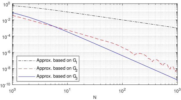
Figure 2: Absolute errors of computation of $T[1]$ using series (32) (black dot-dashed line), (33) (red dashed line) and (34) (solid blue line) as functions of the number of terms used.

References

• [1] N. K. Bary, A treatise on trigonometric series, Vol.1. Pergamon Press, New York, 1964, 553pp.
• [2] H. Begehr and R. Gilbert, Transformations, transmutations and kernel functions, vol. 1–2, Harlow: Longman Scientific & Technical, 1992.
• [3] H. Campos, V. V. Kravchenko, S. M. Torba, Transmutations, L-bases and complete families of solutions of the stationary Schrödinger equation in the plane, J. Math. Anal. Appl. 389 (2) (2012), 1222–1238.
• [4] R. W. Carroll, Transmutation theory and applications, Mathematics Studies, Vol. 117, North-Holland, 1985.
• [5] J. Delsarte, Sur une extension de la formule de Taylor. J Math. Pures et Appl. 17 (1938), 213–230.
• [6] J. Delsarte, Sur certaines transformations fonctionnelles relatives aux équations linéaires aux dérivées partielles du second ordre. C. R. Acad. Sc. 206 (1938), 178–182.
• [7] V. V. Katrakhov, S. M. Sitnik, The transmutation method and boundary value problems for singular differential equations. Contemporary Mathematics. Fundamental Directions. 64:2 (2018), 211–428 (in Russian).
• [8] V. V. Kravchenko, Construction of a transmutation for the one-dimensional Schrödinger operator and a representation for solutions. Appl. Math. Comput., 328 (2018), 75–81.
• [9] V. V. Kravchenko, L. J. Navarro, S. M. Torba, Representation of solutions to the one-dimensional Schrödinger equation in terms of Neumann series of Bessel functions. Appl. Math. Comput. 314 (2017), 173–192.
• [10] V. V. Kravchenko, E. L. Shishkina, S. M. Torba, On a series representation for integral kernels of transmutation operators for perturbed Bessel equations. Math. Notes 104 (2018) No. 3–4, 530–544.
• [11] V. V. Kravchenko and S. M. Torba, Construction of transmutation operators and hyperbolic pseudoanalytic functions, Complex Anal. Oper. Theory 9 (2015), 379–429.
• [12] V. V. Kravchenko, S. M. Torba, R. Castillo-Perez, A Neumann series of Bessel functions representation for solutions of perturbed Bessel equations. Appl. Anal. 97 (5) (2018), 677–704.
• [13] V. V. Kravchenko, S. M. Torba, K. V. Khmelnytskaya, Transmutation operators: construction and applications. Proceedings of the 17th International Conference on Computational and Mathematical Methods in Science and Engineering CMMSE-2017, Cadiz, Andalucia, España, julio 4–8 (2017) pp. 1198–1206, ISBN: 978-84-617-8694-7.
• [14] B. M. Levitan, Inverse Sturm-Liouville problems, VSP, Zeist, 1987.
• [15] V. A. Marchenko, Sturm-Liouville operators and applications: revised edition, AMS Chelsea Publishing, 2011.
• [16] V. A. Yurko, Introduction to the theory of inverse spectral problems. Moscow, Fizmatlit, 2007, 384pp. (Russian). English translation: Method of spectral mappings in the inverse problem theory. VSP, Zeist, 2002.