Learning and Selfconfirming Equilibria in Network Games

Abstract

Consider a set of agents who play a network game repeatedly. Agents may not know the network. They may even be unaware that they are interacting with other agents in a network. Possibly, they just understand that their optimal action depends on an unknown state that is, actually, an aggregate of the actions of their neighbors. Each time, every agent chooses an action that maximizes her instantaneous subjective expected payoff and then updates her beliefs according to what she observes. In particular, we assume that each agent only observes her realized payoff. A steady state of the resulting dynamic is a selfconfirming equilibrium given the assumed feedback. We characterize the structure of the set of selfconfirming equilibria in the given class of network games, we relate selfconfirming and Nash equilibria, and we analyze simple conjectural best-reply paths whose limit points are selfconfirming equilibria.

JEL classification codes: C72, D83, D85.

Keywords: Learning; Selfconfirming equilibrium; Network games; Observability by active players; Shallow conjectures.

1 Introduction

Social networks can be quite complex. Think about friendship networks, networks of people interacting online (such as Twitter, Facebook, Instagram, and so on), or networks of firms (input-output or R&D networks). These networks often consist of thousands (or millions) of agents or firms interacting, and agents rarely know how the network is shaped. In this paper, we provide a novel approach to analyze how incomplete information about the network affects behavior and learning processes. We propose a framework in which agents may ignore how the network affects their payoffs, how the network is shaped, or even that they are interacting in a network.

The standard solution concept used to study the behavior of agents in network games is Nash equilibrium, with the motivation that learning and adaptation converge to a profile of actions in which every player best responds to the actions of the other players. Nash equilibrium action profiles are limit outcomes of learning paths when agents have perfect feedback about the payoff relevant aspects of others’ behavior. Yet, as we shall argue, such perfect feedback hypothesis may be too strong for some social networks applications and, if learning is based on imperfect feedback, non-Nash action profiles may result as the steady-state limits of learning paths. Indeed, such limits under (possibly) imperfect feedback are characterized by the selfconfirming equilibrium concept. With this, we analyze the effects of milder conditions on information feedback. To illustrate, we consider examples where many agents interact and it is plausible to assume that they cannot perfectly observe, whatever action they take, the payoff-relevant aspects of the actions of the others.

In our analysis we assume that the only feedback players receive is their realized payoff. This implies that they do not always observe the payoff-relevant aspects of the actions of others, represented by a payoff state. Yet, each one of them understands how the payoff state and her action determine her payoff and the feedback she is going to receive ex post. We analyze how agents use the feedback they receive to update their conjectures about the payoff state and best respond to them, and we characterize limit behavior under different settings of local and global externalities.

1.1 Introductory example

To be more specific about our modelling approach, let us introduce an example that will guide us through the whole discussion. Consider an online social network with many users, like Twitter, and a simultaneous-moves game in which each user $i$ decides her level of activity $a_{i}\geq 0$ in the social network. The payoff that agents get from their activity depends on the social interaction. We start considering the case in which only local externalities are at play, eventually extending the model to the case in which there are also global externalities. In particular, active user $i$ receives idiosyncratic externalities—that can be positive or negative—from the other users with whom she is in contact in the social network. The externality from user $j$ to user $i$ is proportional to the time that they both spend on the social network, $a_{i}$ and $a_{j}$. Sticking to a quadratic specification, that yields linear best replies, we assume that the payoff function of $i$ is

$$u_{i}(a_{i},\mathbf{a}_{-i})=\alpha_{i}a_{i}-\frac{1}{2}a_{i}^{2}+\displaystyle\sum_{j\in I\backslash\left\{i\right\}}z_{ij}a_{i}a_{j}\text{.}$$ (1)

In equation (1), $I$ is the set of agents, or individuals, in the social network, $a_{i}$ is the level of activity of $i\in I$, $\mathbf{a}_{-i}$ is the profile of activities of all the other users in $I$, and $\alpha_{i}>0$ represents the individual pleasure of $i$ from being active on the social network in isolation, which results in the bliss point of activity in autarchy. For each $j\in I\backslash\left\{i\right\}$, parameter $z_{ij}$ represents the intensity (absolute value) and type (sign) of the externality from $j$ to $i$. We say that $j$ affects $i$, or that $j$ is a peer (or a neighbor) of $i$, if $z_{ij}\neq 0$.

The network described by the matrix $\mathbf{Z}$ of all the $z_{ij}$’s is assumed to be exogenous. As a first approximation, this fits a directed online social network like Twitter or Instagram, where users do not have full control on who follows them.

Consider payoff as expressed in equation (1) (and in (2) below in the introduction). An endogenous directed network in which player $i$ decides who to follow (the $z_{ji}$ entries of matrix $\mathbf{Z}$) but not who is following her (the $z_{ij}$ entries of matrix $\mathbf{Z}$) seems to us in line with our assumption of exogenous network. That is because, in this modification of our model, a player affects the payoff of those that she follows but her payoff is not affected by their choices, including, if the network were endogenous, who they follow. So, endogenizing $\mathbf{Z}$ would mean to endogenize choices (link choices) that are payoff irrelevant for the players.

Under this interpretation, $i$ receives positive or negative externalities from those who follow her proportional to her activity. We do not assume that player $i$ knows all the $z_{ij}$’s. She may not know them either because she cannot observe who is following her, or because she knows her followers but she does not know the sign or intensity of their externality. The payoff of $i$ represents both the pleasure that $i$ gets from participating in the platform and what $i$ can indirectly observe about her own popularity. We consider that $i$ cannot choose the style of what she writes, since she just follows her exogenous nature. In this interpretation, $a_{i}$ represents both the amount of time that $i$ passes on the platform and the amount of posts that $i$ writes, and this can make her more or less appreciated, according to how her style combines with the (typically unobserved) tastes of each of her followers.  In our setting, player $i$ may also set $a_{i}=0$. Indeed, we interpret $\mathbf{Z}$ as a network of opportunities of interaction, with players deciding endogenously whether they want to be active or inactive. When they are inactive, not only the network becomes irrelevant for them, but they also become irrelevant for the payoffs of other players.

The feedback received by agents who have payoff given by (1) is such that, if a player $i$ decides to be inactive ($a_{i}=0$), then she cannot learn anything about the game and about what the others are doing, whereas if she is active ($a_{i}>0$) it is as if she had perfect feedback: indeed, knowing $a_{i}$ and the shape of $u_{i}$, she can infer from her realized payoff the aggregate activity of her peers $\sum_{j\in I\backslash\left\{i\right\}}z_{ij}a_{j}$ (the payoff-relevant aspect of the behavior of others) and understand whether $a_{i}$ was a best reply to it. Inactive players, instead, cannot observe whether inactivity was a best reply to peers’ activity. This simplified framework mimics the fact that, for example, in an online social network active users are surrounded by enough information to have a quasi-perfect feedback about what happens, whereas inactive agents, because they opt out from the network, are likely to ignore relevant information.

We specify what agents observe after their choices because this affects how they update their beliefs, and we are going to analyze learning dynamics and their steady states. To fix ides, we shall refer to the social network Twitter. Twitter user $i$, typically, does not observe the sign of the externalities and the activity of others. However, she gets indirect measures of her level of appreciation that come, for instance, from her conversations and experiences in the real world, where her activity on Twitter affects her social and professional real life. If the players are small firms using Twitter for advertising, they will observe their actual profits. Players of this game may have wrong beliefs about the details of the game they are playing (e.g., the structure of the network, or the value of the parameters) and about the actions of other players. Consequently, they update their beliefs in response to the feedback they receive, which is assumed to be their payoff, and maximize their instantaneous expected payoff given such updated beliefs. This updating process yields learning paths that do not necessarily converge to a Nash equilibrium of the game.

Next we also consider an extra global term in the payoff function:

$$u_{i}(a_{i},\mathbf{a}_{-i})=\alpha_{i}a_{i}-\frac{1}{2}a_{i}^{2}+\displaystyle\sum_{j\in I\backslash\left\{i\right\}}z_{ij}a_{i}a_{j}+\gamma\displaystyle\sum_{k\in I\backslash\left\{i\right\}}a_{k}\text{.}$$ (2)

We can interpret this extra term $\gamma\displaystyle\sum_{k\in I\backslash\left\{i\right\}}a_{k}$ as an additional utility that $i$ gets, regardless of being active or inactive. In this case, what agents can learn from being active or inactive radically changes with respect to the previous case without global externalities, because even an active player may not be able to disentangle what is the contribution of the global term.

We propose an online social network as our leading example, but there are other possible cases in which incomplete information about the network is key. For example, a network of firms, where the feedback is observed profit and actions are levels of production, posted prices, or R&D activities. Many firms are competitors, experiencing local substitutabilities in their choices, some are complementors, and for some of them it may not be clear what kind of strategic interaction is at play. Sometimes, the firm does not know of the set of all its competitors or complementors. Moreover, firms often tend to hide their investment plans and R&D choices to some of their partners, while each firm observes its own profits. In this case, firms ignore important aspects of the network and do not observe ex post the actions of other firms. So, incomplete information plays a critical role and, as we are going to argue, objectively suboptimal choices may be implemented even in a long-run steady state.

1.2 Preview of the model and results

Although we let agents largely ignore the nature and extent of network externalities, we rely on the following minimal maintained assumption: each agent knows how her payoff (utility) and information feedback depend on her action and on a payoff state, which in turn depends on neighbors’ actions in the given network (but the agent may ignore the latter dependence). With this, each agent best responds to her conjecture about the payoff state, observes her realized payoff, and—in equilibrium—her conjecture must be consistent with the feedback received, that is, confirmed. Note that conjectures may be confirmed without being correct. A profile of actions and conjectures satisfying these requirements forms a selfconfirming equilibrium, whereby agents best respond to conjectures that can be wrong, but are nonetheless believed to be true, as they are consistent with the available evidence.

In our analysis, we assume that agents observe only their realized payoff. Given the assumed properties of the payoff functions, it follows that there exists a discontinuity in what agents learn from their feedback about their neighborhood depending on whether they are active (choosing a strictly positive action) or inactive (choosing a null action). In particular, if externalities are only local (i.e., positive or negative peer effects), active players are always able to exactly infer from the feedback the realized payoff state, even if they may have a wrong conjecture about how many neighbors they have or what their neighbors choose. Indeed, we say that in a selfconfirming equilibrium active agents have correct shallow conjectures about the payoff state, but possibly wrong deep conjectures about the parameters and the actions of others. Actually, agents may even be unaware that the payoff state is determined by others within an interactive network structure; in this case, they do not hold deep conjectures. Given that network games without global externalities are easier to analyze and relevent in their own right, we first study this special case and then extend the analysis to games with both local and global externalities.

Absent global externalities, an inactive agent receives uninformative feedback. If—given her conjecture—she finds it subjectively optimal to be inactive, such lack of information about the payoff state creates an “inactivity trap”, allowing her possibly wrong conjecture to persist. This has important consequences for selfconfirming equilibrium action profiles. If being inactive is dominated—e.g., because local externalities are positive and this is known—, then Nash and selfconfirming equilibrium action profiles coincide. However, if there are agents for whom being inactive is not dominated—e.g., due to some negative local externalities—, then any subset of this set of agents may be inactive in some selfconfirming equilibrium. In this case inactivity is a best reply to confirmed, but possibly false conjectures. Specifically, under the assumption that externalities are only local, we characterize selfconfirming equilibrium action profiles as Nash equilibrium profiles of fictitious reduced games where inactive players are absent, augmented by the null actions of the inactive players. We also discuss how the structure of the network adjacency matrix (which may be unknown to the players) determines the existence of such equilibria.

We then study “conjectural best-reply paths” whereby each agent best responds to a shallow conjecture that coincides with the payoff state of the previous period, if it was revealed, or with the confirmed conjecture of the previous period, if the payoff state was not revealed. It follows that the set of inactive agents can only increase, because once an agent becomes inactive she gets uninformative feedback and the conjecture to which she is best replying persists. If such a process converges, the limit must be a selfconfirming equilibrium. Conversely, every selfconfirming equilibrium is—trivially—the limit of a constant conjectural best-reply path. More interestingly, we provide conditions on the adjacency matrix for convergence and stability of such paths. Again, what we find is the possibility of “inactivity traps.” Consider the case of online social networks. If an agent experiences a negative payoff because some of her followers whose externalities toward her are negative played high actions (hence, giving negative feedback online), then she may choose to abstain from interacting. Later, platform conditions may improve, making it objectively profitable to be active, but the now inactive agent cannot observe it.

Models of games on networks have mainly focused on the impact of local externalities, since global ones just change welfare without affecting the best-reply functions. However, when agents observe only their realized payoff, the presence of global externalities may impact the way in which conjectures are confirmed or revised. Recall that in our setting a game is not solely characterized by the best-reply functions, but also by the structure of the payoff/feedback functions. This implies that additional selfconfirming equilibrium (SCE) action profiles are possible compared to the case with only local externalities. Indeed, we show that the SCE action profiles studied for the latter special case correspond to the equilibria of games with local and global externalities, in which agents have correct conjectures about the global aggregate. But there are other SCEs in which conjectures about global aggregates are wrong. For the sake of simplicity, we focus on the case of positive local and global externalities, in which being inactive is dominated. Even in this simple case, agents may have a continuum of confirmed conjectures about the relative size of the two externalities. Indeed, there are multiple SCEs because, even if they are active, players may have false but confirmed conjectures making them choose actions that are not objective best replies. In detail, we find that active agents are not able to perfectly infer the size of the local externality due to the confound induced by the global externality: the realized payoff, a one-dimensional feedback, does not allow to retrieve a two-dimensional (local-global) externality. In particular, since we assume positive externalities, we show that agents’ perception of their role in the network determines whether in a selfconfirming equilibrium they are more or less active than predicted by a Nash equilibrium. Thus, overall activity and (possibly) welfare are higher if agents think that (externalities are positive and that) they are more linked than in reality. If we consider the example of online social networks, this may help explain why firms always try to send to their users messages to make them believe that they are very connected, so as to increase their level of activity. When considering a network of investing firms, we may have under(over)–investment with respect to what would be the optimal, as firms may under(over)–estimate what their neighbors do, without being corrected by the feedback they receive. Even though this equilibria multiplicity can shed light on some interesting phenomena of games with global externalities, we also find an interesting relationship linking the equilibrium action profiles of games with only local externalities and also global ones. In details, the SCE action profiles of a game with only local externalities selects the SCE action profiles of the corresponding game with also global externalities in which conjectures about global externalities are correct.

The paper is structured as follows. In Section 2 we discuss the related literature. Section 3 presents the basic framework and equilibrium concept. In Section 4 we analyze network games with only local externalities, whereas in Section 5 we analyze a more general model that accounts for global externalities. Section 6 concludes.

We devote appendices to proofs and technical results. Appendix A analyzes properties of feedback and selfconfirming equilibria in a class of games including as a special case the linear–quadratic network games that we consider in the main text. In Appendix B we study how equilibria are affected when when the network (or some aspects of it) is commonly known and players are strategically sophisticated. Appendix C reports existing and novel results in linear algebra, that we use to find sufficient conditions for unique and interior Nash equilibria in network games. Appendix D contains the proofs of the results presented in the main text.

2 Related literature

We model interactions through linear–quadratic network games. We focus on this class of games because it has well-known properties, and it has been used for modelling a variety of environments where strategic interaction is local and can be described by a network structure, as surveyed by Zenou (2016) and Bramoullé and Kranton (2016). Moreover, these games belong to the larger class of nice games (Moulin, 1984), for which we provide in Appendix A some general results. Bramoullé et al. (2014) show that other payoff functions lead to the same best-reply functions, hence, to the same Nash equilibria of linear–quadratic network games. However, we focus on selfconfirming equilibria (SCE), and, since realized payoffs affect feedback, the entire payoff function is relevant, not just the corresponding best-reply function. Thus, we rely in our analysis on the specific original payoff function of network games, as introduced in the economic literature by Ballester et al. (2006).

We call “selfconfirming equilibria” the steady states of learning processes when static or dynamic games are played recurrently, independently of the specific assumptions about feedback (monitoring) at the end of each one-period play (see also Battigalli et al., 1992). This concept encompasses what used to be called “conjectural equilibrium” as well as the original “selfconfirming equilibrium” of Fudenberg and Levine (1993). In an SCE, agents best respond to confirmed conjectures that may be inconsistent with sophisticated strategic reasoning. The latter has been added to SCE relating it to rationalizability. See Section IV of Battigalli et al. (2015) and the relevant references therein for a more detailed discussion of different versions of these concepts. Here we focus on SCE, while we analyze SCE with rationalizable conjectures in Appendix B. Lipnowski and Sadler (2019) apply a concept akin to rationalizable SCE of games where feedback about the behavior of others is described by a network topology: agents have correct conjectures about the strategies of their peers (neighbors), but their payoff may depend on the whole strategy profile and it is not observed ex post. We instead assume that agents observe (only) their realized payoff and that the network describes how the payoff of each agent is affected by the actions of other her neighbors (with global externalities, there is also an influence of other players on own payoffs not mediated by the network structure).

McBride (2006) applies SCE to games of network formation with asymmetric information. In his model, agents observe (only) the private information of other agents they link to, and possibly of agents to whom they are indirectly linked. We instead assume that the network is exogenous and actions are activity levels. We allow for information incompleteness, but—with the partial exception of Section 5—we do not assume that agents are necessarily aware of the states of nature (e.g., the possible network structures), hence we do not assume that agents necessarily reason about them. Frick et al. (2022) apply a refinement of rationalizable SCE to analyze a model with asymmetric information and assortative matching. The refinement is obtained by assuming that agents neglect the assortativity of matching when they make inferences from feedback. Foerster et al. (2018) share elements of Lipnowski and Sadler (2019) and of McBride (2006). As in the former, agents observe the behavior of those with whom they are linked; furthermore, they also observe public links. As in the latter, theirs is a model of network formation. They assume that beliefs satisfy a kind of rationalizable SCE condition. Unlike those papers, however, Foerster et al. (2018) do not explicitly analyze the equilibria of a non-cooperative game, but rather adopt a reduced-form notion of stability akin to Jackson and Wolinsky (1996).

3 Framework

3.1 Network games

Consider a finite set of agents (or players) $I$, with cardinality $n=|I|$ and generic element $i$. Agents are located in a network $\mathbf{Z}\in\mathcal{Z}\subset\mathbb{R}^{I\times I}$, where $\mathcal{Z}$ is the compact set of all possible weighted networks, here expressed as adjacency matrices. Each agent $i\in I$ chooses an action $a_{i}$ from a compact interval $A_{i}=[0,\bar{a}_{i}]$. For each $i\in I$, $\mathbf{A}_{-i}:=\times_{j\neq i}A_{j}$ denotes the set of feasible action profiles $\mathbf{a}_{-i}=\left(a_{j}\right)_{j\in I\backslash\{i\}}$ for players different from $i$. For each $i\in I$, we posit two compact intervals $X_{i}:=[\underline{x}_{i},\bar{x}_{i}]\subset\mathbb{R}$ and $Y_{i}:=[0,\bar{y}_{i}]\subset\mathbb{R}_{+}$ of payoff states for $i$, with the interpretation that $i$’s payoff is determined by her action $a_{i}$, the interaction between $a_{i}$ and state $x_{i}$, and the additive term $y_{i}$ according to the quadratic utility function

$$v_{i}:$$ ,

.

(3)

Payoff state $x_{i}$ is determined by the actions of $i$’s neighbors—the agents with non-zero weight in adjacency matrix $\mathbf{Z}$—according to the parameterized linear aggregator

$$\ell_{i}:$$ ,

.

(4)

Since the codomain of $\ell_{i}$ is $[\underline{x}_{i},\bar{x}_{i}]$, we are effectively assuming that

$$\underline{x}_{i}\leq\sum_{j\in N_{i}^{-}}z_{ij}\bar{a}_{j}\text{, }\bar{x}_{i}\geq\sum_{j\in N_{i}^{+}}z_{ij}\bar{a}_{j}$$

for every $\mathbf{Z}\in\mathcal{Z}$, where $N_{i}^{-}:=\left\{j\in I:z_{ij}<0\right\}$ denotes the set of neighbors of player $i$ that have a negative effect on the payoff state of $i$, and $N_{i}^{+}:=\left\{j\in I:z_{ij}>0\right\}$ denotes the set of neighbors of player $i$ that have a positive effect on the payoff state of $i$.

We also posit a compact set $\mathcal{G}\subset\mathbb{R}_{+}$ of nonnegative global externality parameter values. Payoff state $y_{i}$ is a non-strategic global externality determined by all the co-players’ actions according to the proportional aggregator:

$$\begin{tabular}[]{llll}$g_{i}:$&$\mathbf{A}_{-i}\times\mathcal{G}$&$\rightarrow$&$Y_{i}$\\ &$\ \ \ (\mathbf{a}_{-i},\gamma)$&$\mapsto$&$\gamma\displaystyle\sum_{j\neq i}a_{j}$\end{tabular}.$$ (5)

Since the codomain of $g_{i}$ is $[0,\bar{y}_{i}]$, we are assuming that

$$\max\mathcal{G}\displaystyle\sum_{j\neq i}\bar{a}_{j}\leq\bar{y}_{i}$$

The special case of no global externalities obtains if $\bar{y}_{i}=0$.

With this, we derive the parameterized payoff function

$$u_{i}:$$ ,

.

Since $y_{i}$ does not interact with $a_{i}$, $x_{i}=\ell_{i}\left(\mathbf{a}_{-i},\mathbf{Z}\right)$ is the payoff-relevant state that $i$ has to guess in order to choose a subjectively optimal action. We let

$$r_{i}\left(x_{i}\right)=\left\{\begin{tabular}[]{ll}$0$,&if $x_{i}\leq-\alpha_{i}$,\\ $\alpha_{i}+x_{i}$,&if $-\alpha_{i}<x_{i}<\bar{a}_{i}-\alpha_{i}$,\\ $\bar{a}_{i}$,&if $x_{i}\geq\bar{a}_{i}-\alpha_{i}$.\end{tabular}\right.$$ (6)

denote the continuous and piecewise linear best-reply function of player $i\in I$. Note that, since $\alpha_{i}>0$, we may have $r_{i}\left(x_{i}\right)=0$ only if $\underline{x}_{i}<0$.

We assume that the game is repeatedly played by agents maximizing their instantaneous payoff. Each agent $i$ knows her utility function $v_{i}:A_{i}\times X_{i}\times Y_{i}\rightarrow\mathbb{R}$ as specified in eq. (3), hence also its domain $A_{i}\times X_{i}\times Y_{i}=[0,\bar{a}_{i}]\times[\underline{x}_{i},\bar{x}_{i}]\times\left[0,\bar{y}_{i}\right]$ and the “stand-alone” parameter $\alpha_{i}$, but we do not assume that the aggregators parameters $\left(\mathbf{Z},\gamma\right)$ are known. Actually, for most of our analysis it does not even matter that agents understand that payoff states aggregate the actions of others according to eq.s (4) and (5). After each play, agents get an imperfect feedback about the payoff states. Specifically, we assume that each agent observes only her realized utility/payoff. What agent $i$ learns in a given period after choosing action $a_{i}$ and observing her realized payoff $\hat{v}_{i}$ is that $\left(x_{i},y_{i}\right)\in\left\{\left(x_{i}^{\prime},y_{i}^{\prime}\right):v_{i}\left(a_{i},x_{i}^{\prime},y_{i}^{\prime}\right)=\hat{v}_{i}\right\}$, that is,

$$\left(x_{i},y_{i}\right)\in\left\{\begin{tabular}[]{ll}$\left\{\left(x_{i}^{\prime},y_{i}^{\prime}\right):y_{i}^{\prime}=\hat{v}_{i}\right\}$,&if $a_{i}=0$,\\ $\left\{\left(x_{i}^{\prime},y_{i}^{\prime}\right):\alpha_{i}a_{i}-\frac{1}{2}a_{i}^{2}+a_{i}x_{i}^{\prime}+y_{i}^{\prime}=\hat{v}_{i}\right\}$,&if $a_{i}>0$.\end{tabular}\right.$$

In words, if $i$ is inactive she can infer $y_{i}$ but has no clue about $x_{i}$, if she is active she obtains joint information about $y_{i}$ and $x_{i}$ that she cannot disentangle.

If there are no global externalities, that is, if $\bar{y}_{i}=0$, then being inactive reveals nothing, because $v_{i}\left(0,x_{i}\right)=0$ independently of $x_{i}$, while being active reveals that

$$x_{i}=\frac{\hat{v}_{i}-\alpha_{i}a_{i}+\frac{1}{2}a_{i}^{2}}{a_{i}}=\frac{\hat{v}_{i}}{a_{i}}-\alpha_{i}+\frac{1}{2}a_{i}\text{.}$$

With this assumption about feedback, the interactive situation is represented by the mathematical structure

$$NG=\left\langle I,\mathcal{Z},\mathcal{G},\left(A_{i},X_{i},Y_{i},v_{i},\ell_{i},g_{i}\right)_{i\in I}\right\rangle\text{,}$$

determined by eq.s (3), (4), and (5), which we call (parameterized) linear-quadratic network game with just observable payoffs, or simply network game. This structure is summarized in equation (2).

To choose an action, a subjectively rational agent $i$ must have some deterministic or probabilistic conjecture about the payoff state $x_{i}$. Yet, her post-feedback update about $x_{i}$ depends on what she thinks about $y_{i}$, because she gets imperfect joint feedback about both. Therefore, we model how $i$ forms conjectures about $x_{i}$ and $y_{i}$. We refer to conjectures about the states $x_{i}$ and $y_{i}$ as shallow conjectures, as opposed to deep conjectures, which concern the specific network topology $\mathbf{Z}$, the global externality parameter $\gamma$ (when present), and the actions of other players $\mathbf{a}_{-i}$. In our equilibrium analysis, given the continuity of the best-reply function and the connectedness of $X_{i}$ and $Y_{i}$, it is sufficient to focus on deterministic shallow conjectures. Indeed, for each $i\in I$ and every probabilistic conjecture $\mu_{i}\in\Delta\left(X_{i}\times Y_{i}\right)$, there exists a corresponding deterministic conjecture $\left(\hat{x}_{i},\hat{y}_{i}\right)\in X_{i}\times Y_{i}$ that justifies the same action $a_{i}^{\ast}$ as the unique best reply. Deep conjectures are relevant for the analysis of strategic thinking based on common belief in rationality (see Appendix B), but our equilibrium concept does not rely on strategic thinking.

3.2 Selfconfirming equilibrium

We analyze a notion of equilibrium that characterizes the steady states of learning dynamics and therefore relaxes the mutual-best-reply condition of the Nash equilibrium concept. Recall that our approach allows for the possibility of agents being unaware of many aspects of the game. In equilibrium, agents best respond to (deterministic) shallow conjectures consistent with the feedback that they receive given the true parameter values $\left(\mathbf{Z},\gamma\right)$.

Definition 1.

A profile $\left(a_{i}^{\ast},\hat{x}_{i},\hat{y}_{i}\right)_{i\in I}\in\times_{i\in I}\left(A_{i}\times X_{i}\times Y_{i}\right)$ of actions and (shallow) deterministic conjectures is a selfconfirming equilibrium (SCE) at $\left(\mathbf{Z},\gamma\right)$ if, for each $i\in I$,

1. (subjective rationality) $a_{i}^{\ast}=r_{i}\left(\hat{x}_{i}\right)$,

2. (confirmed conjecture) $v_{i}\left(a_{i}^{\ast},\hat{x}_{i},\hat{y}_{i}\right)=v_{i}\left(a_{i}^{\ast},\ell_{i}\left(\mathbf{a}_{-i}^{\ast},\mathbf{Z}\right),g_{i}\left(\mathbf{a}_{-i}^{\ast},\gamma\right)\right)$.

The two conditions require that: 1) each agent best responds to her own conjecture; 2) the conjecture in equilibrium must belong to the ex post information set, so that the expected payoff (feedback) coincides with the realized payoff (feedback) given $a_{i}^{\ast}$, $x_{i}=\ell_{i}\left(\mathbf{a}_{-i}^{\ast},\mathbf{Z}\right)$, and $y_{i}=g_{i}\left(\mathbf{a}_{-i}^{\ast},\gamma\right)$. We say that $\mathbf{a}^{\ast}=\left(a_{i}^{\ast}\right)_{i\in I}$ is a  selfconfirming action profile at $\left(\mathbf{Z},\gamma\right)$ if there exists a corresponding profile of conjectures $\left(\hat{x}_{i},\hat{y}_{i}\right)_{i\in I}$ such that $\left(a_{i}^{\ast},\hat{x}_{i},\hat{y}_{i}\right)_{i\in I}$ is a selfconfirming equilibrium at $\left(\mathbf{Z},\gamma\right)$, and we let $\mathbf{A}_{\mathbf{Z},\gamma}^{SCE}$ denote the set of such action profiles; in the special case of no global externalities, we write $\mathbf{A}_{\mathbf{Z}}^{SCE}$ to ease notation. Also, for any $\mathbf{Z}\in\mathcal{Z}$, we denote by $\mathbf{A}_{\mathbf{Z}}^{NE}$ the set of (pure) Nash equilibria of the game determined by $\mathbf{Z}$ neglecting the non-strategic global externalities, that is,

$$\mathbf{A}_{\mathbf{Z}}^{NE}:=\left\{\mathbf{a}^{\ast}\in\times_{i\in I}A_{i}:\forall i\in I,a_{i}^{\ast}=r_{i}\left(\ell_{i}\left(\mathbf{a}_{-i}^{\ast},\mathbf{Z}\right)\right)\right\}\text{.}$$

Since, for each $\mathbf{Z}$, the joint best-reply function $\mathbf{a}^{\ast}\mapsto\left(r_{i}\left(\ell_{i}\left(\mathbf{a}_{-i}^{\ast},\mathbf{Z}\right)\right)\right)_{i\in I}$ is a continuous self-map on the compact and convex subset $\times_{i\in I}\left[0,\bar{a}_{i}\right]\subseteq\mathbb{R}^{I}$, Brower Fixed Point Theorem implies that a Nash equilibrium exists. Hence, we obtain the existence of selfconfirming equilibria for each $\left(\mathbf{Z},\gamma\right)\in\mathcal{Z\times B}$. Indeed, a Nash equilibrium $\mathbf{a}^{\ast}$ corresponds to a selfconfirming equilibrium with correct conjectures $\left(a_{i}^{\ast},\hat{x}_{i},\hat{y}_{i}\right)_{i\in I}=\left(a_{i}^{\ast},\ell_{i}\left(\mathbf{a}_{-i}^{\ast},\mathbf{Z}\right),g_{i}\left(\mathbf{a}_{-i}^{\ast},\gamma\right)\right)_{i\in I}$. To summarize:

Remark 1.

For every $\mathbf{Z}\in\mathcal{Z}$ and $\gamma\in\mathcal{G}$, there is at least one Nash equilibrium at $\mathbf{Z}$, and every Nash equilibrium at $\mathbf{Z}$ is a selfconfirming action profile at $\left(\mathbf{Z},\gamma\right)$:

$$\forall\ \left(\mathbf{Z},\gamma\right)\in\mathcal{Z}\times\mathcal{G}\text{, }\emptyset\neq\mathbf{A}_{\mathbf{Z}}^{NE}\subseteq\mathbf{A}_{\mathbf{Z},\gamma}^{SCE}.$$

In the next sections we study selfconfirming equilibria and learning, first when there are only local externalities, and then when also global externalities are considered.

4 Local externalities

In this section, we analyze the set of selfconfirming equilibria and the learning paths in linear-quadratic network games with just observable payoffs and without global externalities. Several proofs are derived from the results in Appendix A, which refers to the case of generic network games with feedback, and from the results in Appendix C. The proofs themselves are collected in Appendix D. In subsection 4.1 we relate selfconfirming equilibria to the Nash equilibria of auxiliary reduced games and we classify equilibria according to the set of active agents. In subsection 4.2 we provide properties of $\mathbf{Z}$ that imply uniqueness of active agents’ equilibrium actions. In subsection 4.3 we analyze learning paths.

4.1 Nash equilibrium and structure of the SCE set

Let $I_{0}$ denote the set of players for whom being inactive is justifiable (that is, undominated):

$$I_{0}:=\left\{i\in I:\exists~{}x_{i}\in X_{i},\ r_{i}\left(x_{i}\right)=0\right\}=\left\{i\in I:\alpha_{i}+\underline{x}_{i}\leq 0\right\}\text{.}$$

Also, for each $\mathbf{Z}\in\mathcal{Z}$ and non-empty subset of players $J\subseteq I$, let $\mathbf{A}_{J,\mathbf{Z}}^{NE}$ denote the set of Nash equilibria of the auxiliary game with player set $J$ obtained by imposing $a_{i}=0$ for each $i\in I\backslash J$, that is,

$$\mathbf{A}_{J,\mathbf{Z}}^{NE}=\left\{\mathbf{a}_{J}^{\ast}\in\times_{j\in J}A_{j}:\forall j\in J,a_{j}^{\ast}=r_{j}\left(\ell_{j}\left(\mathbf{a}_{J\backslash\{j\}}^{\ast},\mathbf{0}_{I\backslash J},\mathbf{Z}\right)\right)\right\}\text{,}$$

where $\mathbf{0}_{I\backslash J}\in\mathbb{R}^{I\backslash J}$ is the profile that assigns $0$ to each $i\in I\backslash J$. If $J=\emptyset$, let $\mathbf{A}_{J,\mathbf{Z}}^{NE}=\left\{\varnothing\right\}$ by convention, where $\varnothing$ is the pseudo-action profile such that $\left(\varnothing,\mathbf{0}_{I}\right)=\mathbf{0}_{I}$. We relate the set of selfconfirming equilibria to the sets of Nash equilibria of such auxiliary games.

Proposition 1.

In a linear-quadratic network game with just observable payoffs, for each $\mathbf{Z}\in\mathcal{Z}$, the set of selfconfirming action profiles is

$$\mathbf{A}_{\mathbf{Z}}^{SCE}=\bigcup_{J:I\backslash J\subseteq I_{0}}\mathbf{A}_{J,\mathbf{Z}}^{NE}\times\left\{\mathbf{0}_{I\backslash J}\right\}\text{,}$$

that is, in each selfconfirming action profile $\mathbf{a}^{\ast}$, a subset $I\backslash J$ of players for whom being inactive is justifiable choose $0$, and every other player chooses the best reply to the actions of her co-players. Therefore, in each selfconfirming action profile $\mathbf{a}^{\ast}$ and for each player $i\in I$,

$$a_{i}^{\ast} = 0\Rightarrow\underline{x}_{i}\leq-\alpha_{i}\text{,}$$

$$a_{i}^{\ast} > 0\Rightarrow\left(\alpha_{i}+\sum_{j\in I}z_{ij}a_{j}^{\ast}>0\text{ }\wedge a_{i}^{\ast}=\min\left\{\bar{a}_{i},\alpha_{i}+\sum_{j\in I}z_{ij}a_{j}^{\ast}\right\}\right)\text{.}$$ (7)

Suppose for simplicity that, in every restricted auxiliary game with player set $J$, Nash equilibrium actions are strictly positive (Proposition 2 below provides sufficient conditions). Then in every SCE we can partition the set of agents in two subsets. Agents in $J\subseteq I$ are active, while agents in $I\setminus J$ choose the null action. Start by considering the latter group of agents. They must belong to the set of agents for whom inactivity is justifiable; as such, they choose $0$ as a best reply to a possibly wrong conjecture, and get null payoff independently of others’ actions. Since every conjecture is consistent with this payoff, their conjecture is (trivially) consistent with their feedback. As for agents in $J$, since they choose a strictly positive action, they receive a message that enables them to infer the true payoff state; with this, they necessarily choose the objective best reply to their neighbors’ actions, whether or not they are aware of them. Note that, if being inactive is justifiable for every agent ($I_{0}=I$), then $\mathbf{0}_{I}\in\mathbf{A}_{\mathbf{Z}}^{SCE}$ for every $\mathbf{Z}\in\mathcal{Z}$. In the polar opposite case, being inactive is unjustifiable for every agent ($I_{0}=\emptyset$) and SCE coincides with Nash equilibrium. For example, assume that $\mathbf{Z}=w\mathbf{Z}_{0}$, with $w>0$ and that $\mathbf{Z}_{0}\in\{0,1\}^{I\times I}$. In this context it is natural to also assume that $\min X_{i}\geq 0$, which implies that being inactive is unjustifiable (recall, $\alpha_{i}>0$). This represents the standard case of local complementarities studied by Ballester et al. (2006). If $w\left(n-1\right)<1$, there is a unique Nash equilibrium which is also interior and coincides with the unique SCE action profile.

Thus, the SCE set can be characterized by means of the Nash equilibria of the auxiliary games in which only active agents are considered. If, for example, for every given set $J\subseteq I$ there is a unique Nash equilibrium of the corresponding auxiliary game (Proposition 2 provides sufficient conditions), then $|\mathbf{A}_{\mathbf{Z}}^{SCE}|=2^{|I_{0}|}$, because for each $J$ with $I\backslash J\subseteq I_{0}$ there is exactly one SCE where the set of active agents is $J$. Since each auxiliary game has at least one Nash equilibrium (see Remark 1), $2^{|I_{0}|}$ is a lower bound on the number of SCE’s. If we assume strategic substitutes, then the Nash equilibria for each auxiliary game in which only agents in $J\subseteq I$ may be active, can be characterized as in Bramoullé et al. (2014). Note that in this case, some of the agents in $J$ can be active and some inactive. Appendix A.3 discusses the equilibrium characterization for the general case of non linear-quadratic network games.

Example 1.

Consider Figure 1, representing a network with 4 nodes/players. We set $\alpha_{i}=0.1$ for every $i$. First assume that each arrow represents a positive externality of $0.2$ (and arrows point to the source of the externality), but we allow agents to believe that links may also be a source of negative externality. Then, agents may find it justifiable to be inactive. In this case we have one Nash equilibrium (NE), but 16 possible SCE’s, one for each subset of the players that we allow to be active. Table 1 reports the actions of players in each case (we omit redundant doubletons and singletons). Note that player $3$, when active, always plays the same action $a_{3}=0.1$, because she is not affected by any externality. Other players, instead, when active, play differently according to who else is active.

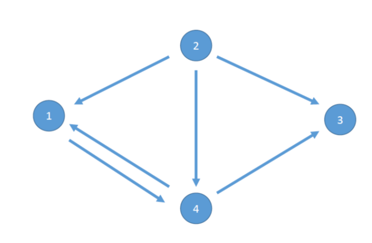
Figure 1: A network with 4 nodes. Every arrow identifies an externality of equal magnitude and sign.

	All	$\{1,2,3\}$	$\{1,2,4\}$	$\{1,3,4\}$	$\{2,3,4\}$	$\{1,2\}$	$\{1,3\}$	$\{1,4\}$	…	$\emptyset$
$a_{1}$	0.1292	0.1	0.125	0.1292	0	0.1	0.1	0.125		0
$a_{2}$	0.1750	0.14	0.15	0	0.144	0.12	0	0		0
$a_{3}$	0.1	0.1	0	0.1	0.1	0	0.1	0		0
$a_{4}$	0.1458	0	0.125	0.1458	0.12	0	0	0.125		0

Table 1: Selfconfirming equilibria of the network from Figure 1, with all positive externalities of $0.2$. Columns are for the subsets of active players. The unique Nash Equilibrium is in bold.

Consider now the same network, but assume that each arrow represents a negative externality of $-0.6$. In this case we have more NE’s (there is no NE where all players are active, but there are 3 NE’s), but less than 16 SCE’s (there are 13), because for some subset $J$ of players (such as $J=I=\{1,2,3,4\}$) there is no SCE in which all its agents are active. Table 2 reports the actions of players in each case (we omit redundant doubletons and singletons).    

	$\mathbf{\{1,2,4\}}$	$\mathbf{\{2,3,4\}}$	$\{1,2\}$	$\mathbf{\{1,3\}}$	$\{1,4\}$	…	$\emptyset$
$a_{1}$	0.0625	0	0.1	0.1	0.0625		0
$a_{2}$	0.025	0.016	0.04	0	0		0
$a_{3}$	0	0.1	0	0.1	0		0
$a_{4}$	0.0625	0.04	0	0	0.0625		0

Table 2: Selfconfirming equilibria of the network from Figure 1, with all negative externalities of $-0.6$. Columns are for the subsets of active players. Nash Equilibria are in bold.

4.2 Relative uniqueness

We list below some properties of the weighted adjacency matrix $\mathbf{Z}$ that will be used throughout the text but are not maintained assumptions. In what follows, we will assume some of these properties to retrieve sufficient conditions for the existence and stability of selfconfirming equilibria. In particular, they imply the uniqueness of selfconfirming equilibrium actions relative to any given set $J$ of active players. We refer to Appendix C for a deeper discussion on these assumptions and their implications.

Assumption 1.

Matrix $\mathbf{Z}$ of size $n$ has bounded values, i.e., for each $i,j\in I$, $|z_{ij}|<\frac{1}{n}$.

Assumption 2.

Matrix $\mathbf{Z}$ has the same sign property, i.e., for each $i,j\in I$, $sign(z_{ij})=sign(z_{ji})$, where the $sign$ function can have values $-1$, $0$ or $1$.

Assumption 3.

Matrix $\mathbf{Z}$ is negative, i.e., for each $i,j\in I$, $z_{ij}<0$.

We recall here that the spectral radius $\rho(\mathbf{Z})$ of $\mathbf{Z}$ is the largest absolute value of its eigenvalues.

Assumption 4.

Matrix $\mathbf{Z}$ is limited, i.e., $\rho(\mathbf{Z})<1$.

In some cases, we can write $\mathbf{Z}=\mathbf{WZ}_{0}$, where $\mathbf{W}$ is a diagonal matrix, and $\mathbf{Z}_{0}\in\{0,1\}^{I\times I}$ is the basic underlying topology of the network. Whenever this is the case, matrix $\mathbf{Z}$ represents a basic network combined with an additional idiosyncratic effect by which every agent $i$ weights the effects of others on her. These effects are modeled by the parameter $w_{i}$. The next assumption adds a symmetry condition on $\mathbf{Z}_{0}$.

Assumption 5.

Matrix $\mathbf{Z}$ is symmetrizable, i.e., it can be written as $\mathbf{Z=WZ}_{0}$, with $\mathbf{W}$ diagonal and $\mathbf{Z}_{0}$ symmetric. Moreover, $\mathbf{W}$ has all strictly positive entries in the diagonal.

Note that if $\mathbf{Z}$ is symmetrizable then all its eigenvalues are real. Moreover, since $\mathbf{W}$ has all strictly positive entries, Assumption 5 implies that the sign condition (Assumption 2) holds.
Our final assumption is discussed in Bramoullé et al. (2014) and combines Assumptions 4 and 5 above.

Assumption 6.

$\mathbf{Z}=\mathbf{WZ}_{0}$ is symmetrizable-limited, i.e., $\mathbf{Z}$ is symmetrizable and the matrix $\bar{\mathbf{Z}}$, whose entries are defined, for each $i,j\in I$, as $\bar{z}_{ij}=z_{0,ij}\sqrt{w_{i}w_{j}}$, is limited.

Our previous results, about the characterization of selfconfirming equilibria, state that we can choose any subset $J\subseteq I_{0}$ of agents and have them inactive in an SCE. However, we cannot ensure that the other agents are active, because their best response in the reduced game could be to stay inactive, since the Nash equilibrium of the reduced game in which only agents in $I\backslash J$ are considered may have both active and inactive agents. The next result goes in the direction of specifying under what sufficient conditions this does not happen. Given the matrix $\mathbf{Z}$, and given $J\subseteq I$, we call $\mathbf{Z}_{J}$ the submatrix which has only rows and columns corresponding to the elements of $J$.

Proposition 2.

Consider a linear-quadratic network game and a subset of players $J\subseteq I$, such that $I\backslash J\subseteq I_{0}$ (that is, $\alpha_{i}+\underline{x}_{i}\leq 0$ for each $i\notin J\,$). Suppose that $\mathbf{Z}_{J}$ satisfies at least one of the three conditions below:

1. it has bounded values (Assumption 1);

2. it is negative and limited (Assumptions 3 and 4);

3. it is symmetrizable–limited (Assumption 6).

Then, we have the following two results:

• the auxiliary game with player set $J$ has a unique and strictly positive Nash equilibrium: $\mathbf{A}_{\mathbf{Z}_{J}}^{NE}=\left\{\mathbf{a}_{J}^{NE}\right\}$ with ${a}_{j}^{NE}>0$ for all $j\in J$;

• $(\mathbf{a}_{J}^{NE},\mathbf{0}_{I\backslash J})$ is a selfconfirming equilibrium at $\mathbf{Z}$.

Proposition 2 provides sufficient conditions to have arbitrary sets of active and inactive players in a selfconfirming equilibrium. In particular, if any of the three conditions is satisfied for every subset of $I$, and if for all players being inactive is justifiable ($I_{0}=I$), then the set of SCE’s has the same cardinality as the power set $2^{I}$, that is $2^{n}$. The first sufficient condition about (sub)matrix $\mathbf{Z}_{J}$ is novel, while the other two were obtained respectively by Ballester et al. (2006) and Stańczak et al. (2006), and by Bramoullé et al. (2014).

We provide here below two examples, one with all positive externalities, the other with mixed externalities.

Example 2.

Consider $n$ players, and a randomly generated network between them, of the type $\mathbf{Z=WZ}_{0}$, obtained from the following generating process. $\mathbf{Z}_{0}$ is undirected, generated by an Erdos and Rényi (1960) process for which each link is i.i.d., and such that its expected number of overall links (i.e., counted in both directions) is $k\cdot n$, for some $k\in\mathbb{R}_{+}$. This means that the expected number of links for each player is $k$. It is well known that this model predicts, as $n$ goes to infinity, that $\mathbf{\ Z}_{0}$ will have null clustering and, with $k\geq 2$, a connected giant component.

$\mathbf{W}$ is a diagonal matrix, such that each element $w_{i}$ in the diagonal is strictly positive and is generated by some i.i.d. random process with mean $\mu$ and variance $\sigma^{2}$. In this case, Füredi and Komlós (1981) prove that the expected highest eigenvalue of $\mathbf{Z}$, as $n$ grows, is

$$\mathbb{E}[\lambda_{1}]=k\mu+\frac{\sigma^{2}}{\mu}+O\left(\frac{1}{\sqrt{n}}\right)\ .$$

Under Assumption 6, as $n$ tends to infinity, $\mathbf{Z}$ is symmetrizable–limited if $\mathbb{E}[\lambda_{1}]<1$, which is equivalent to

$$\frac{\mu-\sigma^{2}}{\mu^{2}}>k\ .$$

Clearly, a necessary condition for the previous inequality is that $\mu>\sigma^{2}$. When this is the case, as $n$ grows to infinity, there always exists a unique NE of the game where all players are active, as stated by Proposition 2.
Note that, since the expected clustering of $\mathbf{Z}_{0}$ goes to $0$, this limiting result excludes the possibility that there is a subset $J$ of players forming a dense sub–network, and a high realization of $w_{i}$’s, such that there does not exist $\mathbf{a}^{\ast}\in\mathbf{A}_{\mathbf{Z}}^{SCE}$, for which $\mathbf{a}^{\ast}=\left\{\mathbf{a}_{J}^{NE}\right\}\times\left\{\mathbf{0}_{I\backslash J}\right\}\text{.}$ In fact, if this were the case, since there are only positive externalities, we would not have an all-active equilibrium for the whole population of $n$ agents.    

Example 3.

Proposition 2 provides alternative sufficient conditions for an interior NE in the auxiliary game with player set $J$. Figure 2 provides an example of game that does not satisfy any of them, but still has a unique interior NE. We set $\alpha_{i}=0.1$ for each player $i$. Every blue arrow represents a positive externality of intensity $0.2$ (so, the blue arrows represent the first case from Example 1). The two red arrows represent negative externalities of intensity $-0.2$. This network game has a unique NE, and 16 SCE’s. Table 3 shows them all (redundant doubletons and singletons are omitted).

	All	$\{1,2,3\}$	$\{1,2,4\}$	$\{1,3,4\}$	$\{2,3,4\}$	$\{1,2\}$	$\{1,3\}$	$\{1,4\}$	$\{2,3\}$	…	$\emptyset$
$a_{1}$	0.1257	0.1	0.125	0.128	0	0.1	0.1	0.125	0		0
$a_{2}$	0.1603	0.1346	0.15	0	0.144	0.12	0	0	0.1154		0
$a_{3}$	0.0412	0.731	0	0.720	0.1	0	0.1	0	0.0729		0
$a_{4}$	0.1336	0	0.125	0.14	0.12	0	0	0.125	0		0

Table 3: Selfconfirming equilibria of the network from Figure 2, with positive (resp., negative) externalities of intensity $0.2$ (resp.,$-0.2$). Columns correspond to subsets of active players. The unique Nash Equilibrium is in bold.

   

Figure 2: A network with 4 nodes. Blue (resp., red) arrows represent positive (resp., negative) externalities.

4.3 Learning paths

Definition 1 of selfconfirming equilibrium and the characterization stated in Proposition 1 identify steady states: if agents’ conjectures are confirmed (not contradicted) by the feedback they receive, these conjectures will not change in the next interactions. However, we may wonder how agents get to play SCE action profiles and if these profiles are stable.

We first point out that SCE has solid learning foundations. The following result is specifically relevant for this paper (see Gilli, 1999 and Chapter 7 of Battigalli et al., 2022). Consider a temporal sequence (path) of action profiles $\left(\mathbf{a}_{t}\right)_{t=0}^{\infty}$. Then, if $\left(\mathbf{a}_{t}\right)_{t=0}^{\infty}$ is consistent with adaptive learning and $\mathbf{a}_{t}\rightarrow\mathbf{a}^{\ast}$, it follows that $\mathbf{a}^{\ast}$ must be a selfconfirming action profile.

To ease the analysis we consider conjectural best-reply paths for shallow conjectures. For each network $\mathbf{Z}$, each period $t\in\mathbb{N}$, and each agent $i\in I$, $a_{i,t}=r_{i}\left(\hat{x}_{i,t}\right)$ is the best reply to $\hat{x}_{i,t}$. After actions are chosen, given the feedback received, agents update their conjectures. If conjectures are confirmed then an agent keeps her previous conjecture, otherwise she updates it using as new conjecture the one that would have been correct in the previous period. Thus,

$$\hat{x}_{i,t+1}=\left\{\begin{array}[]{cc}\hat{x}_{i,t}&\text{if }a_{i,t}=0,\\ \ell_{i}\left(\mathbf{a}_{-i,t},\mathbf{Z}\right)&\text{if }a_{i,t}>0,\end{array}\right.$$ (8)

and, from (6) we obtain

$$a_{i,t+1}=r_{i}\left(\hat{x}_{i,t+1}\right)=\left\{\begin{tabular}[]{ll}$0$,&if $\hat{x}_{i,t}\leq-\alpha_{i}$,\\ $\bar{a}_{i}$,&if $\hat{x}_{i,t+1}\geq\bar{a}_{i}-\alpha_{i}$,\\ $\alpha_{i}+\hat{x}_{i,t+1}$,&otherwise.\end{tabular}\right.$$

We will consider the possibility that the upper bound $\bar{a}_{i}$ is reached only in the analysis of diverging dynamics. Given our assumptions about feedback, being inactive is an absorbing state: if an agent is inactive at time $t$ she will remain so also at time $t+1$. If instead the agent is active ($a_{i,t}>0$), feedback is such that the agent can perfectly infer the payoff state $x_{i,t}=\ell_{i}\left(\mathbf{a}_{-i,t},\mathbf{Z}\right)$, and so she updates conjectures according to (8), which becomes the updated conjectures. This is a conjectural best-reply path. The result cited above implies that if the path described above converges, then it must converge to a selfconfirming equilibrium, i.e., a rest point where players keep repeating their choices.

In this subsection, we analyze the local stability of such rest points (cf. Bramoullé and Kranton, 2007).

Definition 2 (Conjectural best-reply paths).

A sequence of profiles of actions and shallow deterministic conjectures $(\mathbf{a}_{t},\mathbf{\hat{x}}_{t})_{t\in\mathbb{N}_{0}}$ is a conjectural best-reply path if it has the following features:

1. Each player $i\in I$ starts at time $0$ with a belief, and beliefs are represented by a profile of shallow deterministic conjectures $\mathbf{\hat{x}}_{0}=\left(\hat{x}_{i,0}\right)_{i\in I}$.

2. In each period  $t$, players best reply to their conjectures: for each $i\in I$, $a_{i,t}=\max\{\alpha_{i}+\hat{x}_{i,t},0\}$.

3. At the beginning of each period $t+1$, each player $i$ keeps her period–$t$ shallow conjecture if she was inactive, and updates her conjecture to period–$t$ revealed payoff state if she was active, that is, $\hat{x}_{i,t+1}=\frac{u_{i}\left(\mathbf{a}_{t},\mathbf{Z}\right)}{a_{i,t}}-\alpha_{i}+\frac{1}{2}a_{i,t}$.

Observe that the system is deterministic and the initial conditions completely determine the paths. From conditions (7) and (8), the system is not linear because, for each $i\in I$ and $t\in\mathbb{N}_{0}$,

$$\hat{x}_{i,t+1}=\left\{\begin{array}[]{ccc}\hat{x}_{i,t}&\mbox{ if }&\hat{x}_{i,t}\leq-\alpha_{i}\ ,\\ \sum_{j\in I}z_{ij}a_{j,t}&\mbox{ if }&\hat{x}_{i,t}>-\alpha_{i}\ .\end{array}\right.$$

Clearly an SCE of the game is always a rest point of these learning paths. Indeed, every SCE $\left(\mathbf{a}^{\ast},\mathbf{\hat{x}}\right)$ is—trivially—the limit of the constant conjectural best-reply path starting at $(\mathbf{a}_{0},\mathbf{\hat{x}}_{0})=\left(\mathbf{a}^{\ast},\mathbf{\hat{x}}\right)$. Furthermore, the set of inactive agents in a conjectural best-reply path can only increase:

$$I_{0}\left(\mathbf{\hat{x}}_{t}\right)\subseteq I_{0}\left(\mathbf{\hat{x}}_{t+1}\right)\ ,$$

where $I_{0}\left(\mathbf{\hat{x}}\right)$ denotes the set of inactive agents given profile of conjectures $\mathbf{\hat{x}=}\left(\hat{x}_{i}\right)_{i\in I}$.

We now consider the stability of such rest points. Say that a profile of conjectures $\mathbf{\hat{x}}$ justifies action profile $\mathbf{a}^{\ast}$ if, for each $i\in I$, $a_{i}^{\ast}=r_{i}\left(\hat{x}_{i}\right)$.

Definition 3.

A profile $\mathbf{a}^{\ast}\in\mathbf{A}_{\mathbf{Z}}^{SCE}$ is locally stable if there exists a profile of conjectures $\mathbf{\hat{x}}$ such that $(\mathbf{a}^{\ast},\mathbf{\hat{x}})$ is a selfconfirming equilibrium, and if there exists an $\epsilon>0$ such that, for each $\mathbf{\hat{x}}_{0}$ with $\left\|\mathbf{\hat{x}}_{0}-\mathbf{\hat{x}}\right\|<\epsilon$ (where $\left\|\cdot\right\|$ is the Euclidean norm), the conjectural best-reply path, starting at $\mathbf{\hat{x}}_{0}$, has a limit and it is such that $\lim_{t\rightarrow\infty}\mathbf{a}_{t}=\mathbf{a^{*}}$.

Since $(\mathbf{a}_{t},\mathbf{\hat{x}}_{t})_{t\in\mathbb{N}_{0}}$ is determined by the initial conjectures $\mathbf{\hat{x}}_{0}$, we analyze stability with respect to perturbations of $\mathbf{\hat{x}}_{0}$. Our notion of stability with respect to conjectures relates to the standard notion of stability with respect to actions in the following way. First of all, since played actions are justified by some conjectures, the only reason for these actions to change is a perturbation of the justifying conjectures, but this is not a sufficient condition. If all agents are active, the two definitions have the same consequences in terms of stability, since a perturbation with respect to actions happens if and only if every agent’s conjecture is perturbed. Indeed, each active agent $i$ has perfect feedback about $x_{i}$, and always chooses the best reply to neighbors’ actions in previous time step. However, consider an SCE with inactive agents, who choose the null action as a corner solution, that is, whose subjective expected marginal utility for increasing activity is strictly negative. For such agents a small perturbation of their conjectures would not change their null subjective best reply. This is so because inactive agents have imperfect feedback and cannot infer the value of the local externality aggregator. This implies that if an action profile is locally stable with respect to action perturbations, then it is also locally stable under conjectures perturbations, but the converse does not hold. Specifically, forcing inactive agents to be active may lead some of them to be active forever. The two definitions would be equivalent under perfect feedback for all agents. Note finally that a temporary perturbation of shallow conjectures $\mathbf{\hat{x}}_{0}$ has the same effect of a temporary shock in the parameter $\mathbf{\alpha}$. By looking at the first order conditions, they both induce the same effect on agents’ best reply and on payoffs.

Each SCE is characterized by a set of active agents. So, given an action profile $\mathbf{a}=\left(a_{i}\right)_{i\in I}$, let $I_{\mathbf{a}}:=\{i\in I:a_{i}>0\}$ denote the set of active players at profile $\mathbf{a}$. Also let $I_{0}^{\ast}:=\left\{i\in I:\alpha_{i}+\underline{x}_{i}<0\right\}$ (a subset of $I_{0}$) denote the set of agents for whom being inactive is a “corner solution” for a set of conjectures with nonempty interior. For each action profile $\mathbf{a}$, $\mathbf{Z}_{I_{\mathbf{a}}}$ denotes the sub–matrix with rows and columns corresponding to players who are active in $\mathbf{a}$. The following result provides sufficient conditions for a selfconfirming equilibrium to be locally stable.

Proposition 3.

The action profile in a selfconfirming equilibrium $(\mathbf{a}^{\ast},\mathbf{\hat{x}})$ such that $\hat{x}^{i}\neq\alpha_{i}$ for each $i\in I$, is locally stable if

• Assumption 4 holds for matrix $\mathbf{Z}_{I_{\mathbf{a}^{\ast}}}$;

• $I\backslash I_{\mathbf{a}^{\ast}}\subseteq I_{0}^{\ast}$.

Intuitively, consider a sufficiently small perturbation of players’ conjectures. The first condition ensures that active players keep being active and their actions converge back to the unique Nash equilibrium of the auxiliary game with player set $I_{\mathbf{a}^{\ast}}$. The second condition ensures that inactive players keep being inactive. Next, we provide alternative sufficient conditions that allow to find the subsets of active agents associated to SCE’s.

Proposition 4.

Consider the action profile $\mathbf{a}^{\ast}$ in a selfconfirming equilibrium $(\mathbf{a}^{\ast},\mathbf{\hat{x}})$ such that $I\backslash I_{\mathbf{a}^{\ast}}\subseteq I_{0}^{\ast}$ and $\hat{x}^{i}\neq\alpha_{i}$ for each $i\in I$. If $\mathbf{Z}_{I_{\mathbf{a}^{\ast}}}$ satisfies at least one of the three conditions below:

1. it has bounded values (Assumption 1),

2. it is negative and limited (Assumptions 3 and 4),

3. it is limited and symmetrizable (Assumptions 4 and 5),

then $\mathbf{a}^{\ast}$ is locally stable. Moreover, for every $J\subseteq I_{\mathbf{a}^{\ast}}$such that $I\backslash J\subseteq I_{0}^{\ast}$, $\mathbf{a}^{\ast\ast}=(\mathbf{a}_{J}^{NE},\mathbf{0}_{I\backslash J})$ is a locally stable SCE action profile, where $\mathbf{a}_{J}^{NE}$ is the unique and strictly positive Nash equilibrium action profile of the auxiliary game restricted to player set $J$.

The proof is based on results from linear algebra. In fact, if an adjacency matrix satisfies one of the conditions from Proposition 4, then also every submatrix of that matrix satisfies that property.

We know that there may be SCE’s that are not Nash equilibria, because some agents are inactive even if this is not a best response to the actions of others. Proposition 4 provides an additional observation. Under the stated conditions, for any given SCE action profile $\mathbf{a}^{\ast}$ with set of active agents $I_{\mathbf{a}^{\ast}}$, any subset $J\subseteq I_{\mathbf{a}^{\ast}}$ of those agents such that $I\backslash J\subseteq I_{0}^{\ast}$ is associated to a stable SCE where all agents in $J$ are active, and the other agents are inactive.

The following example shows that we can reach SCE’s that are not NE’s also if the initial beliefs induce strictly positive actions for all agents at the beginning of the learning paths.

Example 4.

Consider the case of $4$ players, with the network matrix $\mathbf{Z}\in\{-0.2,0,0.2\}^{I\times I}$ shown in Figure 2, and, for every $i$, $\alpha_{i}=0.1$. This is a case of externalities that can be positive or negative. Figure 3 shows the learning paths of actions that start from different initial conditions. In one case (left panel) the path converges to the unique Nash equilibrium of this game (the dotted lines), in the other (right panel) the path makes a player inactive after two rounds and converges to a selfconfirming equilibrium which is not Nash.    

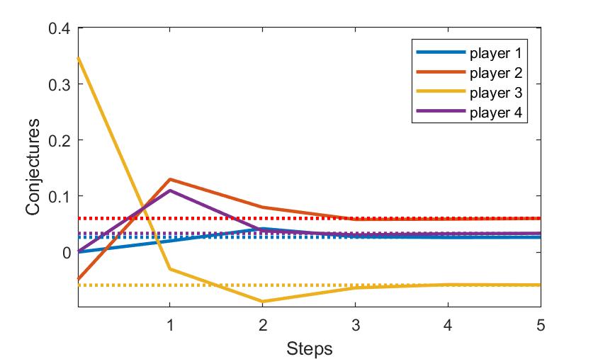
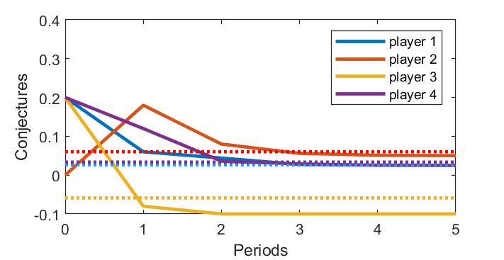
Figure 3: Positive and negative externalities. Starting from different conjectures, given the same network (from Figure 2), the learning process may converge to the unique Nash equilibrium (left panel – dotted lines are the Nash equilibrium) or to an SCE which is not a Nash equilibrium (right panel). For active players, actions are just an upward shift of conjectures of amount $\alpha_{i}$. In the right panel, for the inactive player $3$ the action is $0$ from step $2$ on.

The next example (which does not satisfy the local stability conditions of Proposition 4) shows that convergence may not occur even in a simple case of positive externalities.

Example 5.

Go back to the 4-node network of Example 1 (Figure 1). Even if there are only positive externalities, convergence depends on the magnitude of $w$. If $w<1$, there is convergence. If instead $w\geq 1$, there is divergence. Figure 4 shows two cases, with $w=0.9$ and $w=1$ respectively, starting from the same initial beliefs. Note that the actions of nodes/players 1 and 4 reinforce each other’s beliefs, and this gives rise to an oscillating path of their beliefs. The case of $w=1$, where the amplitude of oscillations remains constant, is actually non–generic.    

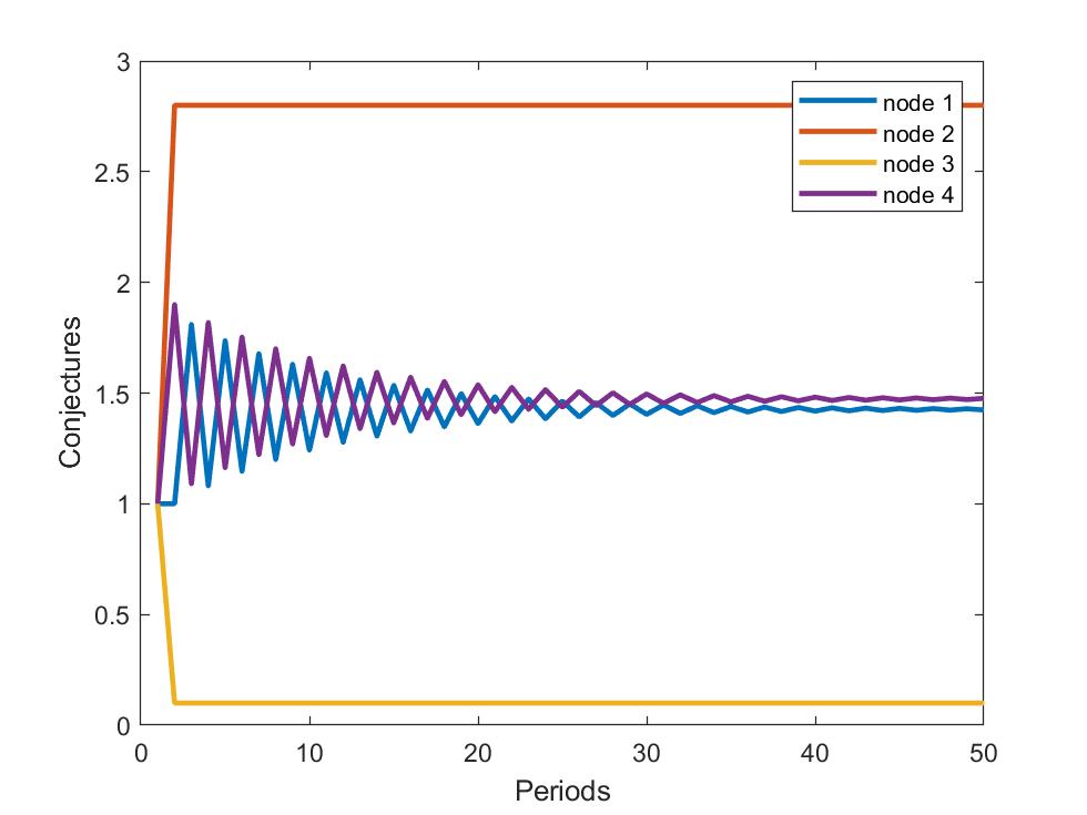
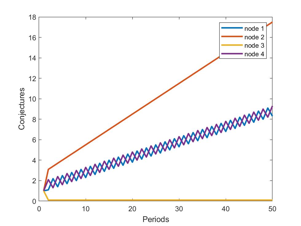
Figure 4: Positive externalities only. Given a network structure (from Figure 1), starting from the same conjectures, the learning path may converge or not depending on the size of $w$: $w=0.9$ in the left panel; $w=1$ in the right panel. Actions are an upward shift of conjectures, of amount $\alpha_{i}$.

5 Local and global externalities

In many applications the feedback that active players receive is not enough to find out the objectively optimal response. Users of online platforms may not understand ex post the objective best response to others’ activityand a firm in a complex market may not be able to infer optimal investment plans by just observing prices. In our context, this means that perfect feedback may not hold even for active players. In particular, this is the case if players just observe their realized payoffs, but there are global externalities, which introduce a confounder. This implies there may be other equilibria besides those analyzed above. Assuming that local externalities are positive, the following analysis yields two important observations. First, players may be more active if they think that they are more linked in the network than they actually are, and this can be welfare improving for the whole society. Second, agents with excessive perceived connectedness may have the effect of preventing the convergence of conjectural best-reply paths to non-corner solutions. Recall Definition 1 (of selfconfirming equilibrium), based on general linear-quadratic network games with just observable payoff (see equations (2)-(5)). We can characterize the set of SCE’s as follows:

Proposition 5.

A profile of actions and conjectures $\left(a_{i}^{\ast},\hat{x}_{i},\hat{y}_{i}\right)_{i\in I}\in\times_{i\in I}\left(A_{i}\times X_{i}\times Y_{i}\right)$ in a linear–quadratic network game with just observable payoffs and global externalities is a selfconfirming equilibrium at $\left(\mathbf{Z},\gamma\right)$ if and only if, for every $i\in I$,

1. $a_{i}^{\ast}=0$ implies $\hat{x}_{i}\in\left[\underline{x}_{i},-\alpha_{i}\right]$ and $\hat{y}_{i}=\gamma\sum_{j\neq i}a_{j}^{\ast}$;

2. $a_{i}^{\ast}>0$ implies $a_{i}^{\ast}=\min\{\alpha_{i}+\hat{x}_{i},\bar{a}_{i}\}$ and $\hat{y}_{i}=\gamma\sum_{k\neq i}a_{k}^{\ast}+a_{i}^{\ast}\left(\sum_{j\neq i}z_{ij}a_{j}^{\ast}-\hat{x}_{i}\right)$.

We discuss how the presence of the global externality term in the utility function changes the characterization of selfconfirming equilibria. Although we maintain the assumption of just observable payoffs, with global externalities it is not anymore the case that active players have perfect feedback about the payoff state. Indeed, for all $i\in I$ and for all pairs of realized externalities $\left(x_{i},y_{i}\right)$, $v_{i}\left(0,x_{i},y_{i}\right)=y_{i}$; thus, inactive players have correct conjectures about the global externality, but may have incorrect conjectures about the local externality. Active players, on the other hand, are not able to determine precisely the relative magnitude of the local effects with respect to the global effects. Given any strictly positive action $a_{i}^{\ast}$, the confirmed conjectures condition yields $(\hat{y}_{i}-y_{i})=a_{i}^{\ast}\left(x_{i}-\hat{x}_{i}\right)$. Then, in equilibrium, if agent $i$ overestimates (underestimates) the local externality, she must compensate this error by underestimating (overestimating) the global externality. Compared to the case of only local externalities, we have that: $(i)$ active agents choose a best response to a (possibly) wrong conjecture about the payoff state; thus, $(ii)$ it is not possible to completely characterize the set of SCE’s by means of Nash equilibria of the auxiliary games restricted to the active players.

Yet, the analysis of Section 4 allows to identify a subset of selfconfirming equilibria, those where agents have correct (shallow) conjectures about the global payoff state.

Remark 2.

Fix $\mathbf{Z}$ and $\gamma$. The set SCE action profiles of the network game with only local externalities is contained in the set of SCE action profiles of the game with local and global externalities, that is, $\mathbf{A}_{\mathbf{Z}}^{SCE}\subseteq\mathbf{A}_{\mathbf{Z},\gamma}^{SCE}$. Specifically, if $\left(a_{i}^{\ast},\hat{x}_{i}\right)_{i\in I}$ is an SCE of the game with only local externalities, then $\left(a_{i}^{\ast},\hat{x}_{i},\hat{y}_{i}\right)_{i\in I}$ with $\hat{y}_{i}=\gamma\sum_{k\neq i}a_{k}^{\ast}$ for each $i\in I$ is an SCE of the game with local and global externalities.

Indeed, by Proposition 1, in profile $\left(a_{i}^{\ast},\hat{x}_{i}\right)_{i\in I}$ each inactive player has a (trivially) confirmed conjecture that makes her choose $0$, and each active player must have a correct conjecture about the local externality. In profile $\left(a_{i}^{\ast},\hat{x}_{i},\hat{y}_{i}\right)_{i\in I}$ conjectures $\left(\hat{y}_{i}\right)_{i\in I}$ about the global externalities are correct by assumption. Thus, by Proposition 5, $\left(a_{i}^{\ast},\hat{x}_{i},\hat{y}_{i}\right)_{i\in I}$ is an SCE.

To ease the following analysis, in the remainder of this whole Section, we assume that (i) each agent $i$ has the same stand-alone parameter $\alpha>0$ and upper bound $\bar{a}$, and (ii) $\gamma>0$. We assume also that (iii) each matrix $\mathbf{Z}\in\mathcal{Z}$ is non–negative, and (iv) either condition 1. or 3. of Proposition 2 is satisfied, so that there exists a unique NE. Finally, (v) we assume that the admissible range of possible best replies for any player has no negative elements and does contain the upper bound $\bar{a}$.

Understanding how conjectures are shaped in a SCE also allows us to shed some light on the efficiency properties of the SCE’s. First of all note that the problem of finding a maximizer of the sum of the utilities is a concave quadratic problem and there exists a bliss point. The presence of positive externalities makes the unique NE Pareto-dominated by other actions profiles. Moreover the presence of a bliss point makes an arbitrary increase of agents’ actions not always welfare improving. Let us analyze these issues in detail.
Given the presence of global externalities, it is straightforward to see that the Nash equilibrium is inefficient. Now, consider an SCE action profile $\mathbf{a}^{SCE}$ (possibly $\mathbf{a}^{NE}$). This action profile is justified by some profile of confirmed conjectures $(\hat{x}_{i},\hat{y}_{i})_{i\in I}$. Then, we can find another SCE, $\mathbf{a^{\prime}}^{SCE}\geq\mathbf{a}^{SCE}$, such that $\mathbf{a^{\prime}}^{SCE}$ yields a higher aggregate payoff than $\mathbf{a}^{SCE}$. A possible way to find such an equilibrium is to decrease, for each $i\in I$, the global externality (shallow) conjecture $\hat{y}_{i}$. To keep the confirmation condition, it is necessary to increase the local (shallow) conjectures $\left(\hat{x}_{i}\right)_{i\in I}$, and thus to increase the best-reply actions. This, in turn, makes the local and global externalities increase. However, this makes it necessary that the local conjectures are further increased, which induces another increase in actions, and so on. The following proposition imposes a condition for the existence of an interior SCE.

Proposition 6.

If, for every pair of agents $(i,j)$ and for every profile of local conjectures $\mathbf{\hat{x}}$, the following inequality is satisfied

$$\sum_{k\in I\backslash\left\{i,j\right\}}z_{ik}\left(\alpha+\hat{x}_{k}\right)-z_{ij}\displaystyle\sum_{h\in I\backslash\left\{i,j\right\}}\left(\alpha+\hat{x}_{h}\right)\alpha\geq 0\ \ ,$$ (9)

then, for every profile of global conjectures $\mathbf{\hat{y}}$ with $\hat{y}_{i}<\bar{a}\bigl{(}\alpha\displaystyle\sum_{k\in I\backslash\left\{i\right\}}z_{ij}+\gamma n\bigr{)}$ for every $i$, there exists a unique SCE with local conjectures $\mathbf{\hat{x}}$ and action profile $\mathbf{a}^{\ast}$, with $a_{i}^{\ast}<\bar{a}$.

The condition of the proposition imposes concavity on some fixed point equations derived from the best replies functions, and then ensure existence and uniqueness of this fixed point. Note that the condition is always satisfied if $\alpha\leq 1$ and $\mathbf{Z}=w\mathbf{Z}_{0}$, with $w>0$, that is: every strictly positive $z_{ij}$ has the same value for each pair of agents $i$ and $j$ in $I$. Otherwise, the larger the number of agents, the more likely it is that the condition is violated for some pair $(i,j)$ for which $z_{ij}$ is high. If the network is composed of just two agents, this condition is always satisfied. The following example illustrates some of the issues just analyzed.

Example 6.

Consider a simple network composed of two agents. Let $z_{ij}z_{ji}=\delta$. For simplicity we assume that $\alpha=\gamma=\delta=0.1$. Figure 5 represents several features of this examples. On the axes we report $\hat{x}_{1}$ and $\hat{x}_{2}$, respectively. The curve $\hat{y}_{1}=0$ represents all the possible $(\hat{x}_{1},\hat{x}_{2})$, such that agent 1 thinks about a null global externalities. Since we know that, in a SCE, $\hat{y}_{1}\geq 0$, then all the feasible conjectures are on the left of this curve, since on the right of $\hat{y}_{1}=0$, we would have negative conjectured global externalities. For the very same reason, only pairs $(\hat{x}_{1},\hat{x}_{2})$ below $\hat{y}_{2}=0$ are consistent with positive conjectured global externality for agent 2. As a result, in a SCE only pairs $(\hat{x}_{1},\hat{x}_{2})$ between the two curves can be observed. The dashed lines show the NE conjectures. As is easy to observe, SCE allows for much higher (and lower too) conjectures, so that larger actions are allowed.
The dashed line represents all the pairs of conjectures delivering the same welfare as the NE. Above this dashed line the welfare is larger than in NE, below this line it is smaller. In this example the SCE with the highest welfare is the top-right kink with the highest possible conjectures (note that, in this case, the bliss point for the welfare is $\hat{x}_{1}=\hat{x}_{2}=0.275$, that is out of the confirmed conjectures area.

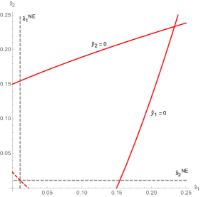
Figure 5: SCE’s for a network of two agents. Parameterization $\alpha=\gamma=\delta=0.1$.

   

To better understand the structure of the equilibrium set, we introduce additional assumptions about what agents know or think they know about the strategic environment. This is a way to restrict their conjectures. We provide some insights along two different dimensions: $i)$ what happens if agents know something about the magnitude of the externalities ? $ii)$ What happens if agents have definite beliefs about the relative size of local with respect to global externality? This last case, that we call perceived centrality will be crucial for the learning dynamics.

5.1 Knowledge of externalities parameters

We assume that $\mathbf{Z}=w\mathbf{Z_{0}}$, where $w>0$, and $\mathbf{Z_{0}\in}\left\{0,1\right\}^{I\times I}$ is the unweighted network. This means that there is a homogeneous positive externality $w$ between all connected players, so that equation (2) becomes:

$$u_{i}(a_{i},\mathbf{a}_{-i},\mathbf{Z})=\alpha_{i}a_{i}-\frac{1}{2}a_{i}^{2}+a_{i}w\sum_{j\in I\backslash\left\{i\right\}}z_{0,ij}a_{j}+\gamma\displaystyle\sum_{k\in I\backslash\left\{i\right\}}a_{k}\ \ .$$ (10)

We do not impose any further restriction over the network structure $\mathbf{Z_{0}}$, but we assume that all agents understand they interact in a network and know $w$ and $\gamma$. Given these assumptions, we need to slightly modify what aggregators and conjectures are. In detail, aggregators about local and global externalities do not internalize $w$ and $\gamma$, respectively, and the conjectures concern the aggregate actions of the neighbors (local) and of all other players (global).

Consider the case in which $\mathbf{Z}=w\mathbf{Z}_{0}^{c}$, where $\mathbf{Z}_{0}^{c}$ is the matrix of the complete basic network (i.e., $z_{0,ij}=1$ for all non-diagonal entries). Note that if the agents conjecture that the network is a complete one, then, for each $i\in I$, $\hat{x}_{i}=\hat{y}_{i}$, and this ensures uniqueness of the SCE. Then the SCE can just be indexed by the conjecture about the local externality. Given $(w,\gamma)$, let $(a_{i}^{c}(w,\gamma),\hat{x}_{i}^{c}(w,\gamma))_{i\in I}$ denote the unique SCE in which, for each $i\in I$, $\hat{x}_{i}^{c}(w,\gamma)$ is the (confirmed) shallow conjecture induced by $\bar{\mu}_{i}^{c}\in\left\{\mathbf{Z}_{0}^{c}\right\}\times\mathbf{A}_{-i}$, that is, a (confirmed) deep conjecture in which $i$ thinks she belongs to a complete network.

Proposition 7.

Consider a linear quadratic network game with global externalities, with $0<w<\frac{1}{n-1}$, and where all agents know $w$ and $\gamma$. Let $\mathbf{a}_{\mathbf{Z}_{0}}^{NE}$ and $\mathbf{a}_{\mathbf{Z}_{0}^{c}}^{NE}$ be the unique Nash equilibria of the game played on $(w\mathbf{Z_{0}},\gamma)$ and $(w\mathbf{Z}_{0}^{c},\gamma)$, respectively. Then, (1) $a_{i}^{c}(w,\gamma)$ is increasing in the ratio $\frac{\gamma}{w}$; (2) $\lim_{\frac{\gamma}{w}\rightarrow 0}\mathbf{a}^{c}(w,\gamma)=\mathbf{a}_{\mathbf{Z}_{0}}^{NE}$; and (3) $\lim_{\frac{\gamma}{w}\rightarrow\infty}\mathbf{a}^{c}(w,\gamma)=\mathbf{a}_{\mathbf{Z}_{0}^{c}}^{NE}$.

So, independently of the basic network $\mathbf{Z}_{0}$, if all players believe to be more linked than they actually are and $\frac{\gamma}{w}$ is large, then the action profile approaches what they would choose in the NE of the game played on the complete network, where every player is linked to every other player.

As it will be clear from Section 5.2, this result implies that the learning paths are self–reinforcing. Players maintain wrong conjectures about the network structure and they infer $\ell_{i}\left(\mathbf{a}_{-i}^{\ast},\mathbf{Z}\right)$ from the payoff that they receive as feedback, using (10). This implies that, converging to an SCE, as they increase their own action they infer a higher $\ell_{i}\left(\mathbf{a}_{-i}^{\ast},\mathbf{Z}\right)$ and a lower $g_{i}\left(\mathbf{a}_{-i}^{\ast},\gamma\right)$, to which they will respond with an even higher action. Nevertheless, this process does not diverge to hit the upper bounds of the action profiles, and it reaches the NE on the complete network.

Proposition 7 is a limiting result. However, for some networks where NE’s and SCE’s can be easily computed analytically, we can show that the actions of an SCE converge rapidly to the actions of the NE for the complete network as $\gamma/w$ becomes large. Figure 6 shows how this happens when every player has the same number of links (regular network) and when there is a central player and every other player is linked only to her (star network).

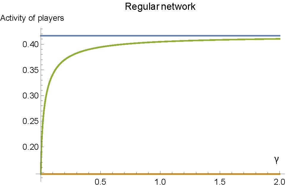
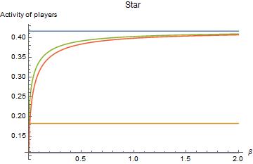
Figure 6: The panels show the SCE common activity level as a function of parameter $\gamma$ when each agent thinks she is connected to every other agent. Both cases have parameters $\alpha=0.1$, $w=0.04$ and $n=20$. The left panel is for the regular network with common degree 8: in blue we have the action that would be played in the NE of the complete network; in yellow the NE of the regular network; in green the SCE action. The right panel is for the star network: in blue we have the action that would be played in the NE of the complete network; in yellow and purple the NE action profiles for the center and the spokes, respectively, in the star network; in green and red the SCE action profile for the center and the spokes, respectively.

In the Introduction we discussed the possible application of our model to online social networks, where the provider may have the possibility to affect the beliefs of the consumers. The previous result applies to the case where consumers know the value of the parameters $w$ and $\gamma$, and their overall number $n$. If we further assume that the profits of the provider are positively correlated with the overall activity on the platform, the provider may have an incentive to make people feel more connected than they actually are. So, if $\frac{\gamma}{w}$ is large (that is, in our interpretation, most of the payoff for the consumers is obtained from using the platform per se, and not from actual interaction), and if these parameters are known to the users, companies make more profit by letting players think that they have a lot of followers. With this application in mind, in the end of this section we will extend the discussion about the implications of biased beliefs on aggregate welfare.

Proposition 7 is based on the assumption that players know the values of $\gamma$ and $w$. However, if they have wrong beliefs about $\gamma$, overestimating it, their actions would even exceed those of the NE of the complete network. This is shown in the next example, where agents do not know the true value of $\gamma$ and, overestimating the ratio between local and global externalities, they play actions that are much above the action that they would play in the NE of the complete network.

Example 7.

Consider three agents in a star network (i.e., a line). Let agent 2 be the center. Then, for every SCE, $\ell_{2}\left(\mathbf{a}_{-2}^{\ast},\mathbf{Z}\right)$ is proportional to $g_{2}\left(\mathbf{a}_{-2}^{\ast},\gamma\right)$, always with the same ratio $\frac{\gamma}{w}$, while this is not true for agents $1$ and $3$. We assume that each agent thinks that the network is complete, so every $i\in I$ thinks that $\ell_{i}\left(\mathbf{a}_{-i}^{\ast},\mathbf{Z}\right)$ is proportional to $g_{i}\left(\mathbf{a}_{-i}^{\ast},\gamma\right)$. In this case agents $1$ and $3$ believe to be more linked than they actually are. Table 4 provides the Nash equilibria for the actual network and for the complete network, and the selfconfirming equilibrium actions for for some specification of the parameters.

	Line NE	Complete Network NE	SCE
$a_{1}$	0.130	0.167	1.569
$a_{2}$	0.152	0.167	1.679
$a_{3}$	0.130	0.167	1.569

Table 4: Simulations for the case of $\alpha=0.1$, $w=0.2$, and $\gamma=1$. Columns refer to 1) Nash Equilibrium of the line network; 2) Nash equilibrium of complete network; 3) SCE in the line network in which each $i\in I$ believes that $\ell_{i}\left(\mathbf{a}_{-i}^{\ast},\mathbf{Z}\right)=\frac{\gamma}{w}g_{i}\left(\mathbf{a}_{-i}^{\ast},\gamma\right)$.

This numerical exercise shows that, when agents overestimate the impact of local externalities, we get a multiplier effect that makes SCE actions increase at a level even larger than what would be predicted in a complete network by Nash equilibrium. This follows from how agents misinterpret their feedback. In particular, thinking to be in a complete network makes agents $1$ and $3$ overestimate local externalities. Take for instance agent $1$. Given any $\mathbf{a}_{-1}$, she chooses a subjective best reply higher than the objective best reply since she overestimates the local externality. This high action has the effect of increasing the global externality term for agent $3$. Agent $3$, by overestimating the local externality, partly attributes this higher global externality to the local externality term, and chooses an action larger than predicted by Nash equilibrium. The choice of agent $3$ increases in turn the global externality perceived by agent $1$, and so on. At the same time agent $2$, as neighbors choose higher actions, increases her own action level. This effect goes on and gives rise to a multiplier effect. The limit of such a conjectural best reply path is selfconfirming equilibrium in which actions are almost ten times larger than the complete network NE actions    

We call $c_{i}:=\frac{\hat{x}_{i}}{\hat{y}_{i}}$ the conjectured ratio of player $i$ with respect to local and global externalities. Then, given a profile $(c_{i})_{i\in I}$, one can rewrite the SCE conditions as a non-linear system of $n$ equations in $n$ unknowns solved either for $(\hat{x}_{i})_{i\in I}$ or $(\hat{y}_{i})_{i\in I}$, and characterize the set of SCE’s given the imposed restrictions. This is what we will use in the next section when studying the learning paths.

We can think of conjectured ratio $c_{i}$ as the perceived centrality of player $i$. For each player, this parameter describes what she thinks to be the share of the activity in her neighborhood with respect to the sum of all the actions of the population. This perceived share has a strong relationship with the Bonacich centrality. If there is a unique Nash equilibrium $\mathbf{a}^{\ast}$ of the game, where all actions are strictly positive, we have, for each $i\in I$,

$$a_{i}^{\ast}=\alpha+x_{i}=\alpha+\sum_{j\in I\backslash\left\{i\right\}}z_{ij}a_{j}^{\ast}\ .$$

The profile of Bonacich centrality measures $\mathbf{b}$ is the unique solution of the linear system

$$\forall i\in I\text{, }b_{i}=\alpha+\sum_{j\in I\backslash\left\{i\right\}}z_{ij}b_{j}\ .$$

So, when beliefs are correct, as in the Nash equilibrium, we have that, for each $i\in I$, $b_{i}=a_{i}^{\ast}$, $y_{i}=\gamma\displaystyle\sum_{k\in I\backslash\left\{i\right\}}a^{*}_{k}$ and $c_{i}=\frac{b_{i}-\alpha}{y_{i}}$.
Now, in the Nash equilibrium we have also that, for each $i$ and $j$, $\frac{1}{y_{i}}-\frac{1}{y_{j}}=\gamma\frac{a_{i}^{\ast}-a_{j}^{\ast}}{y_{i}y_{j}}$. If the number $n$ of players is large, for each $i$ and $j$,  $y_{i}$ and $y_{j}$ grow and the difference $\frac{1}{y_{i}}-\frac{1}{y_{j}}$ approaches $0$ faster than $\frac{1}{y_{i}}$ and than $\frac{1}{y_{j}}$. We can express this writing $\frac{1}{y_{i}}\simeq\frac{1}{y_{j}}$, because as $n$ grows both $\frac{1}{y_{i}}$ and $\frac{1}{y_{j}}$ are of another order of magnitude with respect to $\frac{1}{y_{i}}-\frac{1}{y_{j}}$, and so every $c_{i}$ is roughly the same linear rescaling of $b_{i}$.  Our perceived centrality can then be interpreted, with a good approximation, as the belief that player $i$ has, as a node in a large network, about her Bonacich centrality.

5.2 Learning with global externalities

We now study conjectural best reply paths with global externalities. To simplify the analysis we assume, for each agent, a fixed conjectured ratio. Differently from Section 5.1, we do not assume agents to know anything about the parameters characterizing the strategic environment.
At each time, there are infinitely many profiles of feasible pairs $\left(\hat{x}_{i,t},\hat{y}_{i,t}\right)_{i\in I}$ consistent with feedback. For each $i\in I$, and each time $t\in\mathbb{N}$, let $m_{i,t}=f_{i}\left(a_{i,t},x_{i,t},y_{i,t}\right)=u_{i}(a_{i,t},\mathbf{a}_{-i,t},\mathbf{Z},\gamma)$ be the message agent $i$ receives. Then, given message $m_{i,t-1}$, and considering that agents perfectly recall their past actions, $\hat{y}_{i,t}$ is uniquely determined as a function of $\hat{x}_{i,t}$. In particular, if at each time period $t$ agent $i$’s conjectures $\hat{x}_{i,t}$ and $\hat{y}_{i,t}$ are consistent with the message received at the previous period, we obtain

$$\hat{y}_{i,t+1}=m_{i,t}-\alpha a_{i,t}+\frac{1}{2}\left(a_{i,t}\right)^{2}-a_{i,t}\hat{x}_{i,t+1}\ .$$

Then, we can focus on the path of $\hat{x}_{i,t}$, given by

$$\hat{x}_{i,t+1}=\frac{m_{i,t}-\hat{y}_{i,t+1}}{a_{i,t}}-\alpha+\frac{1}{2}a_{i,t}\ \ .$$ (11)

In this case, active agents do not have perfect feedback, because players test a two–dimensional conjecture with a feedback, the payoff, that has a single dimension. This brings also indeterminacy to the updating rule that players use. To avoid bifurcations at each time period $t$, we need to use simplifying assumptions on conjectures. We define for each $i\in I$ and every $t\in\mathbb{N}_{0}$

$$c_{i,t}:=\frac{\hat{x}_{i,t}}{\hat{y}_{i,t}},$$ (12)

and in the following we assume that this conjectured ratio is constant along paths of learning dynamics for each player $i$.

Assumption 7.

For each $i\in I$ and for each $t\in\mathbb{N}$, $c_{i,t}=c_{i,t+1}=c_{i}$.

From equation (11), and expressing the message as the observed payoff, we get the following learning path, for each agent at each time period:

$$\hat{x}_{i,t+1}=x_{i,t}+\frac{y_{i,t}}{a_{i,t}}-\frac{\hat{y}_{i,t+1}}{a_{i,t}}\ ,$$ (13)

where $x_{i,t}$ and $y_{i,t}$ are the true realized values of the payoff states. Plugging in $c_{i}=\frac{\hat{x}_{i,t}}{\hat{y}_{i,t}}$ we get, for each $t$ and $i$,

$$\hat{x}_{i,t+1}=\frac{c_{i}}{1+c_{i}a_{i,t}}\left(a_{i,t}x_{i,t}+y_{i,t}\right)\ .$$ (14)

Note that the true ratio of player $i$ at time $t$ is

$$c_{i,t}^{\prime}:=\frac{x_{i,t}}{y_{i,t}}\ \ ,$$

with $c_{i,t}^{\prime}\in\left[0,\frac{\sum_{j\neq i}z_{ij}}{\gamma}\right]$. For this reason, we also assume that the conjectured ratio of each player $i$ is such that $c_{i}\in\left(0,\frac{\sum_{j\neq i}z_{ij}}{\gamma}\right]$, and this specifies the set of all admissible conjectured ratios.

The learning dynamic from (13), then, can be written as

$$\hat{x}_{i,t+1}=c_{i}y_{i,t}\frac{a_{i,t}^{\ast}c_{i,t}^{\prime}+1}{a_{i,t}^{\ast}c_{i}+1}\ \ ,$$ (15)

which implies that the conjecture $\hat{x}_{i,t+1}$ is correct only when $c_{i}=c_{i,t}^{\prime}$.

We look at best responses $a_{i,t+1}=\alpha+\hat{x}_{i,t+1}$, and study the existence and characterization of the steady state of this learning process. Recall that $y_{i,t}=\gamma\sum_{j\neq i}a_{j,t}$. To find a fixed point we look at the system of $n$ equations, one for each $i$,

$$H_{i}(\mathbf{a}^{\ast},\mathbf{c},\gamma,\mathbf{Z}):=\alpha+c_{i}\left(\gamma\sum_{j\neq i}a_{j}^{\ast}\right)\frac{a_{i}^{\ast}c_{i}^{\prime}+1}{a_{i}^{\ast}c_{i}+1}-a_{i}^{\ast}=0\ \ .$$ (16)

For comparison, we also study the system of equations that provide the Nash Equilibrium of this network game, that is, for each $i$:

$$F_{i}(\mathbf{a}^{\ast},\mathbf{Z}):=\alpha+\sum_{j\neq i}z_{ij}a_{j}^{\ast}-a_{i}^{\ast}=0\ \ .$$ (17)

Let $\mathcal{A}\subset[\alpha,\infty)^{I}$ denote the set of the solutions of system (16). We have the following result.

Proposition 8.

If the system defined by (17) admits a solution $\mathbf{a}^{\ast}$ with non-negative entries, then for each profile $\mathbf{c}$ of conjectured ratios also the system defined by (16) admits a solution. Moreover, there is a homeomorphism $\Phi$ between the set of all profiles $\mathbf{c}$ and $\mathcal{A}$. The homeomorphism $\Phi$ is strictly monotone with respect to the lattice order of the domain of all profiles $\mathbf{c}$ and the codomain $\mathcal{A}$.

The assumption of non-negative solutions implies a unique NE of the game, and we refer to Proposition 2 for sufficient conditions for uniqueness. This result provides information only on the steady states of our learning paths. It is important because it establishes a one–to–one function between profiles of conjectured ratios and SCEs: there is one and only one SCE strategy profile for each profile $\mathbf{c}$ but there may SCEs that do not result from the hypothesized learning paths. The homeomorphism also provides continuity on the initial parameters, as a marginal change in the conjectured ratios will result in a marginal change in the resulting SCE, even if this function may be highly non–linear, as shown in the example below.

Example 8.

Under the conditions of Proposition 9, we use equation (14) to express learning paths converging to the SCE implicitly defined by (16). This allows us to provide a graphical illustration of Proposition 8, for the case of three nodes. We do this for the case of a line network (where each of the two links is bidirectional), and for the case of a complete network. We consider equation (10), with $\gamma=1$ and $w=0.2$. Figure 7 shows the results. We can start from any pattern of conjectured ratios for the three nodes. The left panel shows the profile of conjectured ratios when at least one node has maximal conjectured ratio (the three faces of the cube have different colors, according to which node has the maximal centrality). The central panel shows the corresponding SCE conjecture profile $\mathbf{\hat{{x}}}$ when the network is a line (the node that has conjectured ratio 1 in the red dots is the central node). The right panel shows the corresponding SCE conjecture profile $\mathbf{\hat{{x}}}$ when the network is a complete triangle. The figure suggests that homeomorphism $\Phi$ (from Proposition 8) is highly non–linear, because of the self-reinforcement process in beliefs that we discussed in Example 7. The figure also shows that, as stated by Proposition 8, homeomorphism $\Phi$ respects the lattice order on the two sets.    

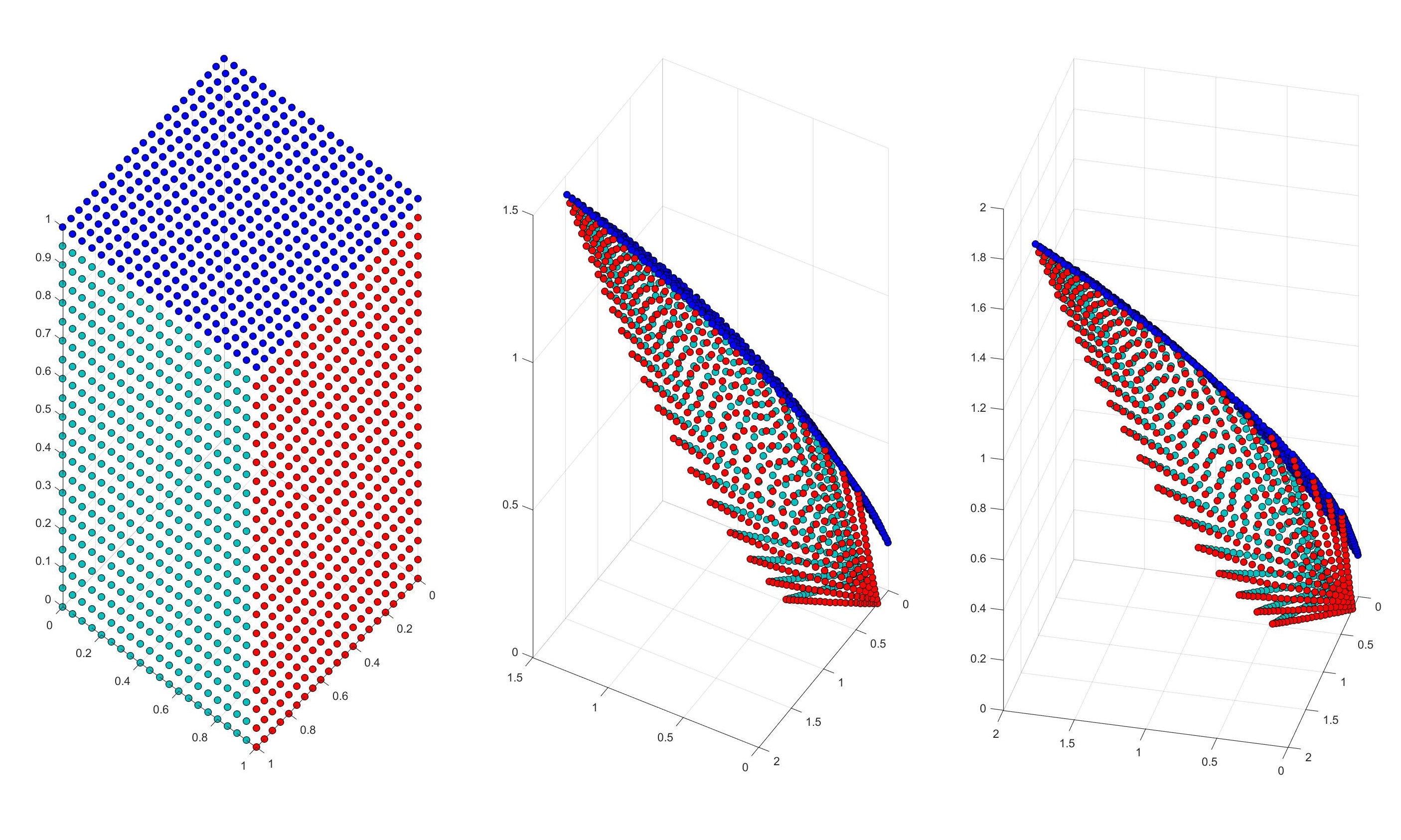
Figure 7: Simulations showing the homeomorphism of Proposition 9 for the case of 3 nodes, as discussed in Example 8. The left panel shows vectors of conjectured ratios. The central panel shows the corresponding SCE conjecture profile $\hat{\mathbf{x}}$ when the network is a line (the node that has conjectured ratio 1 in the red dots is the central node). The right panel shows the corresponding SCE conjecture profile $\hat{\mathbf{x}}$ when the network is a complete triangle.

Monotonicity implies that increasing the conjectured ratio of one player will have a weakly monotonic effect on all the actions of that player and other players in the corresponding SCE. A final caveat to remember is that the homeomorphism is implied by the particular learning path that we are assuming, which is based on constant conjectured ratios. Considering the paths in this special case, in the following proposition we show that if local and global externalities are not too large, the learning paths always converge.

Proposition 9.

If, for each player $i\in I$, $0<c_{i}\gamma(n-1)<\sum_{j\neq i}z_{ij}<2$, then the paths defined by the learning paths (15) always converge to the unique solution of (16), which is locally stable.

It should be noted that, in a game with just local externalities, where $\gamma=0$, the assumptions of Proposition 9 are more general than assuming that $|\sum_{j\neq i}z_{ij}|<1$, which in turn implies that Assumption 4 holds and hence that the learning paths converge. That is because we are focusing on a precise learning path in which players act as if global externalities were present. Moreover, in a game with $\gamma>0$, if for some players the conjectured ratios are too high, the learning paths defined by (16) may not converge to an interior solution, but may hit instead the upper boundaries of the feasible action profiles.

Proposition 8 tells us that a non-negative shift in each conjectured ratio will always result in a non-negative shift of each agent’s action in the resulting SCE. However, Proposition 9 gives an implicit warning. Too high conjectured ratios may imply that the sufficient conditions for stability are lost, and convergence to the corresponding SCE may not occur. Note also that, summing up equation (2) for all the players, the aggregate welfare is maximized if $\mathbf{a}^{\ast}$ solves the following linear system of equalities

$$\forall i\in I\text{, \ }a_{i}^{\ast}=\alpha+(n-1)\gamma+\sum_{j\in I\backslash\left\{i\right\}}(z_{ij}+z_{ij})a_{j}^{\ast}\ .$$

To better understand this aspect, consider the online social networks application we often referred to. The results of this last subsection apply to the case where consumers do not know the parameters of the model and their own total number, but have only a conjecture about the ratio of the benefits from just using the platform, and from the actual strategic interaction on the platform. Social platforms like Facebook and Twitter often provide information to users about the activity of their peers. The social platform Reddit does not show to users their followers, but only a measure of popularity called karma. A rationale for this marketing strategy may be that these companies want to change the beliefs of players, making them feel more important (i.e., more followed) in the social network. Even a benevolent social planner may want to set the conjectured ratios to the level for which the social optimum is achieved. However, according to our model, if conjectured ratios are too high, the learning paths may diverge. For example, in the context of the model and from the assumptions of Proposition 9 a conjectured ratio is too high as soon as $c_{i}\geq\frac{\sum_{j\neq i}z_{ij}}{\gamma(n-1)}$, because in this case learning can lead to SCE where the activity of some player $i$ hits her upper bound $a_{i}$ and the strategy profile is inefficiently high for the players.

This is shown in the following example.

Example 9.

We replicate the same exercise that we did in Example 8, but only for the case of the complete triangle. However we do it for a wider range of conjectured ratios. Figure 8 shows that in this case there may be combinations of conjectured ratios that prevent convergence of the learning paths to interior equilibria.    

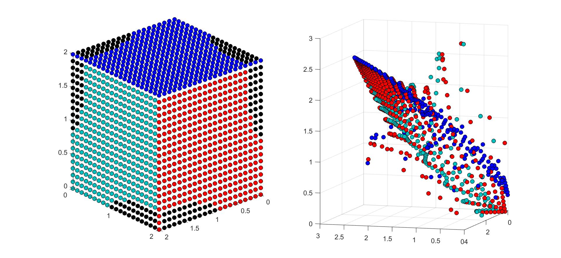
Figure 8: Simulations showing the homeomorphism of Proposition 9 for the case of 3 nodes, as discussed in Example 9. The left panel shows vectors of conjectured ratios. With respect to Figure 7, we allow for higher values of conjectured ratios. Black dots represent cases for which the learning dynamics diverge. The right panel shows the corresponding SCE conjecture profile $\hat{\mathbf{x}}$ when the network is a complete triangle, and when the learning dynamics are converging.

6 Conclusion

In this paper we offer a novel approach to network games. A key application of network games is in modelling large societies with millions of nodes and non regular distributions of connections. It is natural to assume that players may ignore the complete structure of the network; this prevents them from performing sophisticated strategic reasoning possibly leading to a Nash equilibrium. Instead, they just best respond to some subjective beliefs affected by the information feedback they receive. We analyze simple conjectural best-reply paths and show that in some cases they converge to stable Nash equilibria. However, we also characterize those situations in which stable action profiles are not Nash equilibria, but rather selfconfirming equilibrium action profiles in which some (if not all) players have wrong beliefs and yet the feedback they receive is consistent with such beliefs. We also show that, in the presence of global externalities, simple biases in the perception of position in the network may lead players to play action profiles that are far from the Nash equilibria of the game.

One natural application of this approach is to directed online social platforms like  Twitter  and Instagram, where links need not to be reciprocated. Using a linear–quadratic structure for the payoff function we have also laid the ground for a tractable welfare analysis of the model. However, policy implications are not straightforward if we want to consider the long run benefits of connections and not only the instantaneous payoffs of the users of those platforms.

The analysis in Appendix B also provides a first account of the strategic reasoning that agents can perform given some commonly known features of the network. For example, we use known results about rationalizability to show that, if the network game has strategic complementarities, there is common knowledge of the game, and the Nash equilibrium is unique, then sophisticated strategic reasoning leads to the unique NE, whereas the results differ when actions are strategic substitutes.

Appendix A Selfconfirming equilibria in parameterized nice games with aggregators

In this section we develop a more general analysis of selfconfirming equilibria in a class of games that contains the linear-quadratic network games with just observable payoffs studied in the main text. To ease reading, we make this section self-contained, repeating some definitions from the main text. We write this section focusing on local externalities. This because the analysis that follows mainly concerns best-replys, that are not affected by the presence of global externalities, so that all the considerations about best-replys in this section also apply to the case of the presence of global externalities.

A parameterized nice game with aggregators and feedback is a structure

$$G=\left\langle I,\mathcal{Z},\left(A_{i},\ell_{i},v_{i},f_{i}\right)_{i\in I}\right\rangle$$

where

• $I$ is the finite players set, with cardinality $n=\left|I\right|$ and generic element $i$.

• $\mathcal{Z}\subseteq\mathbb{R}^{m}$ is a compact parameter space.

• $A_{i}=\left[0,\bar{a}_{i}\right]\subseteq\mathbb{R}_{+}$, a compact interval, is the action space of player $i$ with generic element $a_{i}\in A_{i}$.

• $X_{i}=\left[\underline{x}_{i},\bar{x}_{i}\right]\subseteq\mathbb{R}$, a compact interval, is the space of payoff states for $i$.

• $\ell_{i}:\mathbf{A}_{-i}\times\mathcal{Z}\rightarrow X_{i}$ (where $\mathbf{A}_{-i}=\times_{j\in I\backslash\{i\}}A_{j}$) is a continuous parameterized aggregator of the actions of $i$’s co-players such that its range $\ell_{i}\left(\mathbf{A}_{-i}\times\mathcal{Z}\right)$ is connected.

• $v_{i}:A_{i}\times X_{i}\rightarrow\mathbb{R}$ is the utility function of player $i$, which is strictly quasi-concave in $a_{i}$ and continuous, and from which we derive the parameterized payoff function

  $$u_{i}:$$ ,

  .

  Thus, $x_{i}=\ell_{i}\left(\mathbf{a}_{-i},\mathbf{Z}\right)$ is the payoff–relevant state that $i$ has to guess in order to choose a subjectively optimal action. With this, for each $\mathbf{Z}\in\mathcal{Z}$, $\left\langle I,\left(A_{i},u_{i,\mathbf{Z}}\right)_{i\in I}\right\rangle$ is a nice game (cf. Moulin 1984), and $\left\langle I,\mathcal{Z},\left(A_{i},u_{i}\right)_{i\in I}\right\rangle$ is a parameterized nice game. We let

  $$r_{i}:$$

  denote the best-reply function of player $i$. The Maximum theorem implies that $r_{i}$ is continuous.

• Let $M\subseteq\mathbb{R}$ be a set of “messages,” $f_{i}:A_{i}\times X_{i}\rightarrow M$ is a continuous feedback function that describes what $i$ observes (a “message,” e.g., a monetary outcome) after taking any action $a_{i}$ given any payoff state $x_{i}$.

On top of the formal assumptions stated above, we maintain the following minimal informal assumption about players’ knowledge of the game:

• Each player $i$ knows $v_{i}$ and $f_{i}$.

Unless we explicitly say otherwise, we instead do not assume that $i$ necessarily knows $\mathbf{Z}$, or function $\ell_{i}$, or even that $i$ understands that her payoff is affected by the actions of other players. However, since $i$ knows the feedback function $f_{i}:A_{i}\times X_{i}\rightarrow M$ and the action she takes, what $i$ infers about the payoff state $x_{i}$ after she has taken action $a_{i}$ and observed message $m$ is that

$$x_{i}\in f_{i,a_{i}}^{-1}\left(m\right):=\left\{x_{i}^{\prime}:f_{i}\left(a_{i},x_{i}^{\prime}\right)=m\right\}.$$

A.1 Conjectures

If player $i$ only knows the feedback function $f_{i}$, but does not know how the payoff state $x_{i}$ is determined, then she just forms a conjecture about $x_{i}$. If instead $i$ knows that $x_{i}$ is determined by the actions of others given parameter $\mathbf{Z}$ through the aggregator $\ell_{i}$, then $i$ forms a conjecture about $\left(\mathbf{a}_{-i},\mathbf{Z}\right)$.

Definition 4.

A shallow conjecture for $i\in I$ is a probability measure $\mu_{i}\in\Delta\left(X_{i}\right)$. A deep conjecture for $i$ is a probability measure $\bar{\mu}_{i}\in\Delta\left(\mathbf{A}_{-i}\times\mathcal{Z}\right)$. An action $a_{i}^{\ast}$ is justifiable if there exists a shallow conjecture $\mu_{i}$ such that

$$a_{i}^{\ast}\in\operatorname*{argmax}_{a_{i}\in A_{i}}\int_{X_{i}}v_{i}\left(a_{i},x_{i}\right)\mu_{i}\left(\mathrm{d}x_{i}\right)\text{;}$$

in this case we say that $\mu_{i}$ justifies $a_{i}^{\ast}$. Similarly, we say that deep conjecture $\bar{\mu}_{i}\in\Delta\left(\mathbf{A}_{-i}\times\mathcal{Z}\right)$ justifies $a_{i}^{\ast}$ if the shallow conjecture induced by $\bar{\mu}_{i}$ ($\mu_{i}=\bar{\mu}_{i}\circ\ell_{i}^{-1}\in\Delta\left(X_{i}\right)$) justifies $a_{i}^{\ast}$.

The following lemma summarizes well known results about nice games (see, e.g., Battigalli et al., 2022) and some straightforward consequences for the more structured class of nice games with aggregators considered here. We include the proof to make the exposition self-contained.

Lemma 1.

The best-reply function $r_{i}:X_{i}\rightarrow A_{i}$ is continuous, hence its range $r_{i}\left(X_{i}\right)$ is a compact interval, just like $X_{i}$. Furthermore, for each $a_{i}^{\ast}\in A_{i}$, the following are equivalent:

• $a_{i}^{\ast}$ is justifiable,

• $a_{i}^{\ast}\in r_{i}\left(X_{i}\right)$ (that is, $a_{i}^{\ast}$ is justified by a deterministic shallow conjecture),

• there is no $a_{i}$ such that $v_{i}\left(a_{i}^{\ast},x_{i}\right)<v_{i}\left(a_{i},x_{i}\right)$ for all $x_{i}\in X_{i}$ (that is, $a_{i}^{\ast}$ is not dominated by any other pure action).

Proof. With a slight abuse of notation, we let $r_{i}\left(\mu_{i}\right)$ denote the set of best replies to (shallow) conjecture $\mu_{i}$:

$$r_{i}\left(\mu_{i}\right):=\arg\max_{a_{i}\in A_{i}}\int_{X_{i}}v_{i}\left(a_{i},x_{i}\right)\mu_{i}\left(\mathrm{d}x_{i}\right)\text{.}$$

By the Maximum theorem $\mu_{i}\mapsto r_{i}\left(\mu_{i}\right)$ has a closed graph, which—under the stated assumptions—is equivalent to upper hemi-continuity. By strict quasi-concavity, the restriction of the best-reply correspondence to the domain $X_{i}$ of deterministic conjectures is single-valued; hence, it must be a continuous function.

Fix any closed (hence, compact) sub-interval $C\subseteq X_{i}$. Let $ND_{i,p}\left(C\right)$ denote the set of actions that are not strictly dominated by other pure actions. By inspection of the definitions, it holds that

$$r_{i}\left(C\right)\subseteq r_{i}\left(\Delta\left(C\right)\right)\subseteq ND_{i,p}\left(C\right)\text{.}$$

We prove that $ND_{i,p}\left(C\right)\subseteq r_{i}\left(C\right)$, that is, $A_{i}\backslash r_{i}\left(C\right)\subseteq A_{i}\backslash ND_{i,p}\left(C\right)$, which therefore implies the thesis. Since $r_{i}$ is a continuous function on $X_{i}\supseteq C$ and $C$ is compact and connected, $r_{i}\left(C\right)$ is compact and connected as well, hence, it is a compact interval. Therefore, it is enough to show that all the actions below $\min r_{i}\left(C\right)$ or above $\max r_{i}\left(C\right)$ are dominated. Fix any $a_{i}<\min r_{i}\left(C\right)$, by strict quasi-concavity,

$$\forall x_{i}\in C\text{, }v_{i}\left(a_{i},x_{i}\right)<v_{i}\left(\min r_{i}\left(C\right),x_{i}\right)\leq v_{i}\left(r_{i}\left(x_{i}\right),x_{i}\right)\text{.}$$

Therefore, every $a_{i}<\min r_{i}\left(C\right)$ is strictly dominated by $\min$ $r_{i}\left(C\right)$. A similar argument shows that every $a_{i}>\max r_{i}\left(C\right)$ is strictly dominated by $\max r_{i}\left(C\right)$. Since there are no other actions outside $r_{i}\left(C\right)$, this concludes the proof. $\blacksquare$

Corollary 1.

Suppose that the aggregator $\ell_{i}$ is onto. Then, an action of player $i$ is justifiable if an only if it is justified by a deterministic (Dirac) deep conjecture.

Proof. The “if” part is trivial. For the “only if” part, fix a justifiable action $a_{i}^{\ast}$ arbitrarily. By Lemma 1, there is some $x_{i}\in X_{i}$ such that $a_{i}^{\ast}=r_{i}\left(x_{i}\right)$. Since the aggregator $\ell_{i}$ is onto, there is some $\left(\mathbf{a}_{-i},\mathbf{Z}\right)\in\ell_{i}^{-1}\left(x_{i}\right)$ such that

$$a_{i}^{\ast}\in\arg\max_{a_{i}\in A_{i}}u_{i}\left(a_{i},\mathbf{a}_{-i},\mathbf{Z}\right)\text{.}$$

Hence $a_{i}^{\ast}$ is justified by the deep conjecture $\delta_{\left(\mathbf{a}_{-i},\mathbf{Z}\right)}$, that is, the Dirac measure supported by $\left(\mathbf{a}_{-i},\mathbf{Z}\right)$. $\blacksquare$

With this, from now on we mostly restrict our attention to (shallow, or deep) deterministic conjectures.

A.2 Feedback properties

Definition 5.

Feedback $f_{i}$ satisfies observable payoffs (OP) relative to $v_{i}$ if there is a function $\bar{v}_{i}:A_{i}\times M\rightarrow\mathbb{R}$ such that

$$v_{i}\left(a_{i},x_{i}\right)=\bar{v}_{i}\left(a_{i},f_{i}\left(a_{i},x_{i}\right)\right)$$

for all $\left(a_{i},x_{i}\right)\in A_{i}\times X_{i}$; if the section $\bar{v}_{i,a_{i}}$ is injective for each $a_{i}\in A_{i}$, then we say that $f_{i}$ satisfies just observable payoffs (JOP) relative to $v_{i}$. Game $G$ satisfies (just) observable payoffs if, for each player $i\in I$, feedback $f_{i}$ satisfies (J)OP relative to $v_{i}$.

If $f_{i}$ satisfies JOP, we may assume without loss of generality that $f_{i}=v_{i}$, because, for each action $a_{i}$, the partitions of $X_{i}$ induced by the preimages of $v_{i,a_{i}}$ and $f_{i,a_{i}}$ coincide:

Remark 3.

Feedback $f_{i}$ satisfies JOP relative to $v_{i}$ if and only if

$$\forall a_{i}\in A_{i}\text{, }\left\{v_{i,a_{i}}^{-1}\left(u\right)\right\}_{u\in v_{i,a_{i}}\left(X_{i}\right)}=\left\{f_{i,a_{i}}^{-1}\left(m\right)\right\}_{m\in f_{i,a_{i}}\left(X_{i}\right)}\text{.}$$ (18)

Proof. (Only if) Fix $a_{i}\in A_{i}$. Since $f_{i}$ satisfies JOP relative to $v_{i}$, $v_{i,a_{i}}\left(X_{i}\right)=\left(\bar{v}_{i,a_{i}}\circ f_{i,a_{i}}\right)\left(X_{i}\right)$ (by OP), for each $u\in v_{i,a_{i}}\left(X_{i}\right)$ there is a unique message $m_{a_{i},u}=\bar{v}_{i,a_{i}}^{-1}\left(u\right)$ (by injectivity of $\bar{v}_{i,a_{i}}$), and

$$v_{i,a_{i}}^{-1}\left(u\right) = \left\{x_{i}\in X_{i}:v_{i}\left(a_{i},x_{i}\right)=u\right\}$$

$$= \left\{x_{i}\in X_{i}:\bar{v}_{i}\left(a_{i},f_{i}\left(a_{i},x_{i}\right)\right)=u\right\}$$

$$= \left\{x_{i}\in X_{i}:f_{i}\left(a_{i},x_{i}\right)=m_{a_{i},u}\right\}=f_{i,a_{i}}^{-1}\left(m_{a_{i},u}\right)\text{,}$$

which implies eq. (18).

(If) Suppose that eq. (18) holds. For every $a_{i}\in A_{i}$ and $m\in f_{i,a_{i}}\left(X_{i}\right)$ select some $\xi_{i}\left(a_{i},m\right)\in f_{i,a_{i}}^{-1}\left(m\right)$. Let

$$D:=\bigcup_{a_{i}\in A_{i}}\left\{a_{i}\right\}\times f_{i,a_{i}}\left(X_{i}\right).$$

With this,

$$\xi_{i}:D\rightarrow X_{i}$$

is a well defined function. Domain $D$ is the set of action-message pairs for which the definition of $\bar{v}_{i}$ matters. Define $\bar{v}_{i}$ as follows:

$$\bar{v}_{i}\left(a_{i},m\right)=\left\{\begin{tabular}[]{ll}$v_{i}\left(a_{i},\xi_{i}\left(a_{i},m\right)\right)$&if $\left(a_{i},m\right)\in D$,\\ $0$&otherwise.\end{tabular}\right.$$

By construction, eq. (18) implies that

$$\forall\left(a_{i},x_{i}\right)\in A_{i}\times X_{i}\text{, }\bar{v}_{i}\left(a_{i},f_{i}\left(a_{i},x_{i}\right)\right)=v_{i}\left(a_{i},x_{i}\right)\text{.}$$

Hence, OP holds. Furthermore, for all $a_{i}\in A_{i}$, $m^{\prime},m^{\prime\prime}\in f_{a_{i}}\left(X_{i}\right)$,

$$m^{\prime}\neq m^{\prime\prime}\Rightarrow \xi_{i}\left(a_{i},m^{\prime}\right)\neq\xi_{i}\left(a_{i},m^{\prime\prime}\right)$$

$$\Rightarrow v_{i}\left(a_{i},\xi_{i}\left(a_{i},m^{\prime}\right)\right)\neq v_{i}\left(a_{i},\xi_{i}\left(a_{i},m^{\prime\prime}\right)\right)$$

$$\Rightarrow \bar{v}_{i}\left(a_{i},m^{\prime}\right)\neq\bar{v}_{i}\left(a_{i},m^{\prime\prime}\right)$$

where the first and the second implications follow from eq. (18) ($\xi_{i}\left(a_{i},m^{\prime}\right)$ and $\xi_{i}\left(a_{i},m^{\prime\prime}\right)$ belong to different cells of the coincident partitions, hence yield different utilities), and the third holds by construction. Therefore, $\bar{v}_{i,a_{i}}$ is injective for every $a_{i}$, which means that JOP holds. $\blacksquare$

Definition 6.

Feedback $f_{i}$ satisfies observability if and only if $i$ is active (OiffA) if section $f_{i,a_{i}}$ is injective for each $a_{i}>0$ and constant for $a_{i}=0$. Game $G$ satisfies observability by active players if OiffA holds for each $i$.

Remark 4.

If a network game is linear-quadratic and satisfies just observable payoffs, then it satisfies observability by active players.

Proof. By Remark 3 JOP implies that, for each $a_{i}\in A_{i}$,

$$\left\{v_{i,a_{i}}^{-1}\left(u\right)\right\}_{u\in v_{i,a_{i}}\left(X_{i}\right)}=\left\{f_{i,a_{i}}^{-1}\left(m\right)\right\}_{m\in f_{i,a_{i}}\left(X_{i}\right)}\text{.}$$

The linear-quadratic form of $v_{i}$ implies that, for every $x_{i}\in X_{i}$,

$$v_{i,0}^{-1}\left(v_{i,0}\left(x_{i}\right)\right)=X_{i}\ ,$$

$$\forall a_{i}>0,v_{i,a_{i}}^{-1}\left(v_{i,a_{i}}\left(x_{i}\right)\right)=\left\{x_{i}\right\}\text{.}$$

These equalities imply that $f_{i,0}$ is constant and $f_{i,a_{i}}$ is injective for $a_{i}>0$, that is, $NG$ satisfies observability by active players. $\blacksquare$

Definition 7.

Feedback $f_{i}$ satisfies own-action independence (OAI) of feedback about the state if, for all justifiable actions $a_{i}^{\ast},a_{i}^{o}$ and all payoff states $\hat{x}_{i},x_{i}$,

$$f_{i}\left(a_{i}^{\ast},\hat{x}_{i}\right)=f_{i}\left(a_{i}^{\ast},x_{i}\right)\Rightarrow f_{i}\left(a_{i}^{o},\hat{x}_{i}\right)=f_{i}\left(a_{i}^{o},x_{i}\right)\text{.}$$

Game $G$ satisfies own-action independence of feedback about the state if, for each player $i\in I$, feedback $f_{i}$ satisfies OAI.

In other words, OAI says that if player $i$ cannot distinguish between two payoff states $\hat{x}_{i}$ and $x_{i}$ when she chooses some given justifiable action $a_{i}^{\ast}$, then she cannot distinguish between these two states when he chooses any other justifiable action $a_{i}^{o}$. This is equivalent to requiring that the partitions of $X_{i}$ of the form $\left\{f_{i,a_{i}}^{-1}\left(m\right)\right\}_{m\in f_{i,a_{i}}\left(X_{i}\right)}$ coincide across justifiable actions, i.e. across actions $a_{i}\in r_{i}\left(X_{i}\right)$ (see Lemma 1).

The following lemma—which holds for any game, not just nice games—states that, under payoff observability and own-action independence, an action is justified by a confirmed conjecture if and only if it is a best reply to the actual payoff state:

Lemma 2.

If $f_{i}$ satisfies observable payoffs relative to $v_{i}$ and own-action independence of feedback about the state, then for all $\left(a_{i}^{\ast},x_{i}\right)\in A_{i}\times X_{i}$ the following are equivalent:

1. there is some $\hat{x}_{i}\in X_{i}$ such that $a_{i}^{\ast}\in\arg\max_{a_{i}\in A_{i}}v_{i}\left(a_{i},\hat{x}_{i}\right)$ and $f_{i}\left(a_{i}^{\ast},\hat{x}_{i}\right)=f_{i}\left(a_{i}^{\ast},x_{i}\right)$,

2. $a_{i}^{\ast}\in\arg\max_{a_{i}\in A_{i}}v_{i}\left(a_{i},x_{i}\right)$.

Proof. (Cf. Battigalli et al., 2015, Battigalli et al., 2022) It is obvious that 2 implies 1 independently of the properties of $f_{i}$. To prove that 1 implies 2 under the stated assumptions, suppose that $f_{i}$ satisfies OP-OAI and let $\hat{x}_{i}$ be such that 1 holds. Let $a_{i}^{o}$ be a best reply to the actual state $x_{i}$. We must show that also $a_{i}^{\ast}$ is a best reply to $x_{i}$. Note that both $a_{i}^{\ast}$ and $a_{i}^{o}$ are justifiable; hence, by OAI, $f_{i}\left(a_{i}^{\ast},\hat{x}_{i}\right)=f_{i}\left(a_{i}^{\ast},x_{i}\right)$ implies $f_{i}\left(a_{i}^{o},\hat{x}_{i}\right)=f_{i}\left(a_{i}^{o},x_{i}\right)$. Using OP, condition 1, and OAI as shown in the following chain of equalities and inequalities, we obtain

$$v_{i}\left(a_{i}^{\ast},x_{i}\right)\overset{(\mathrm{OP})}{=}\bar{v}_{i}\left(a_{i}^{\ast},f_{i}\left(a_{i}^{\ast},x_{i}\right)\right)\overset{(\mathrm{1})}{=}\bar{v}_{i}\left(a_{i}^{\ast},f_{i}\left(a_{i}^{\ast},\hat{x}_{i}\right)\right)\overset{(\mathrm{OP})}{=}v_{i}\left(a_{i}^{\ast},\hat{x}_{i}\right)\overset{(\mathrm{1})}{\geq}$$

$$v_{i}\left(a_{i}^{o},\hat{x}_{i}\right)\overset{(\mathrm{OP})}{=}\bar{v}_{i}\left(a_{i}^{o},f_{i}\left(a_{i}^{o},\hat{x}_{i}\right)\right)\overset{(\mathrm{1,OAI})}{=}\bar{v}_{i}\left(a_{i}^{o},f_{i}\left(a_{i}^{o},x_{i}\right)\right)\overset{(\mathrm{OP})}{=}v_{i}\left(a_{i}^{o},x_{i}\right)\text{.}$$

Since $a^{o}$ is a best reply to $x_{i}$ and $v_{i}\left(a_{i}^{\ast},x_{i}\right)\geq v_{i}\left(a_{i}^{o},x_{i}\right)$, it must be the case that also $a_{i}^{\ast}$ is a best reply to $x_{i}$. $\blacksquare$

Corollary 2.

Suppose that the parameterized nice game with aggregators and feedback $G$ satisfies observable payoffs and own-action independence of feedback about the state, then the sets of selfconfirming action profiles and Nash equilibrium action profiles coincide for each $\mathbf{Z}$:

$$\forall\mathbf{Z}\in\mathcal{Z}\text{, }\mathbf{A}_{\mathbf{Z}}^{SCE}=\mathbf{A}_{\mathbf{Z}}^{NE}\text{.}$$

Proof By Remark 1, we only have to show that $\mathbf{A}_{\mathbf{Z}}^{SCE}\subseteq\mathbf{A}_{\mathbf{Z}}^{NE}$. Fix any $\mathbf{a}^{\ast}=\left(a_{i}^{\ast}\right)_{i\in I}\in\mathbf{A}_{\mathbf{Z}}^{SCE}$ and any player $i$. By definition of SCE and by Lemma 1, there is some $\hat{x}_{i}\in X_{i}$ such that $a_{i}^{\ast}\in r_{i}\left(\hat{x}_{i}\right)$ and $f_{i}\left(a_{i}^{\ast},\hat{x}_{i}\right)=f_{i}\left(a_{i}^{\ast},\ell_{i}\left(\mathbf{a}_{-i}^{\ast},\mathbf{Z}\right)\right)$. By Lemma 2 $a_{i}^{\ast}\in r_{i}\left(\ell_{i}\left(\mathbf{a}_{-i}^{\ast},\mathbf{Z}\right)\right)$. This holds for each $i$, hence $\mathbf{a}^{\ast}\in\mathbf{A}_{\mathbf{Z}}^{NE}$. $\blacksquare$

Corollary 2 provides sufficient conditions for the equivalence between SCE and NE action profiles. Next, we give sufficient conditions that allow a characterization of $\mathbf{A}_{\mathbf{Z}}^{SCE}$ by means of Nash equilibria of auxiliary games.

A.3 Equilibrium characterization

If $a_{i}\in[0,\bar{a}_{i}]$ is interpreted as an activity level (e.g., effort) by player $i$, then it makes sense to say that $i$ is active if $a_{i}>0$ and inactive otherwise. Let $I_{0}$ denote the set of players for whom being inactive is justifiable. Note that, by Lemma 1,

$$I_{0}=\left\{i\in I:\min r_{i}\left(X_{i}\right)=0\right\}\text{.}$$

Also, for each $\mathbf{Z}\in\mathcal{Z}$ and non-empty subset of players $J\subseteq I$, let $\mathbf{A}_{J,\mathbf{Z}}^{NE}$ denote the set of Nash equilibria of the auxiliary game with players set $J$ obtained by letting $a_{i}=0$ for each $i\in I\backslash J$, that is,

$$\mathbf{A}_{J,\mathbf{Z}}^{NE}=\left\{\mathbf{a}_{J}^{\ast}\in\times_{j\in J}A_{j}:\forall j\in J,a_{j}^{\ast}=r_{j}\left(\ell_{j}\left(\mathbf{a}_{J\backslash\{j\}}^{\ast},\mathbf{0}_{I\backslash J},\mathbf{Z}\right)\right)\right\}\text{,}$$

where $\mathbf{0}_{I\backslash J}\in\mathbb{R}^{I\backslash J}$ is the profile that assigns $0$ to each $i\in I\backslash J$. If $J=\emptyset$, let $\mathbf{A}_{J,\mathbf{Z}}^{NE}=\left\{\varnothing\right\}$ by convention, where $\varnothing$ is the pseudo-action profile such that $\left(\varnothing,\mathbf{0}_{I}\right)=\mathbf{0}_{I}$.

Lemma 3.

Suppose that the parameterized nice game with aggregators and feedback $G$ satisfies observability by active players. Then, for each $\mathbf{Z}$, the set of selfconfirming action profiles is

$$\mathbf{A}_{\mathbf{Z}}^{SCE}=\bigcup_{J:I\backslash J\subseteq I_{0}}\mathbf{A}_{J,\mathbf{Z}}^{NE}\times\left\{\mathbf{0}_{I\backslash J}\right\}\text{.}$$

Proof  Fix $\mathbf{a}^{\ast}$ and let $J$ be the set of players $i$ such that $a_{i}^{\ast}>0$. Fix $\mathbf{Z}\in\mathcal{Z}$ arbitrarily. Suppose that $\mathbf{a}^{\ast}\in$ $\mathbf{A}_{\mathbf{Z}}^{SCE}$ and fix any $i\in I$. If $a_{i}^{\ast}=0$, then $0$ is justifiable for $i$, that is $i\in I_{0}$. If $a_{i}^{\ast}>0$, observability by active players implies that $f_{i,a_{i}^{\ast}}$ is injective, that is, action $a_{i}^{\ast}$ reveals the payoff state, which implies that the (shallow) conjecture justifying $a_{i}^{\ast}$ is correct: $a_{i}^{\ast}=r_{i}\left(\ell_{i}\left(\mathbf{a}_{-i}^{\ast},\mathbf{Z}\right)\right)$. Hence $\mathbf{a}^{\ast}_{J}\in\mathbf{A}^{NE}_{J,\mathbf{Z}}$. Thus, $\mathbf{a}^{\ast}=\left(\mathbf{a}_{J}^{\ast},\mathbf{a}_{I\backslash J}^{\ast}\right)$ is such that $a_{i}^{\ast}=0$ for each $i\in I\backslash J\subseteq I_{0}$, and $a_{j}^{\ast}=r_{j}\left(\ell_{j}\left(\mathbf{a}_{J\backslash\{j\}}^{\ast},\mathbf{0}_{I\backslash J},\mathbf{Z}\right)\right)>0$ for each $j\in J$. Hence,

$$\mathbf{a}^{\ast}=\left(\mathbf{a}_{J}^{\ast},\mathbf{a}_{I\backslash J}^{\ast}\right)\in\mathbf{A}_{J,\mathbf{Z}}^{NE}\times\left\{\mathbf{0}_{I\backslash J}\right\}\text{ with }I\backslash J\subseteq I_{0}\text{.}$$

Let $I\backslash J\subseteq I_{0}$ and $\left(\mathbf{a}_{J}^{\ast},\mathbf{a}_{I\backslash J}^{\ast}\right)\in\mathbf{A}_{J,\mathbf{Z}}^{NE}\times\left\{\mathbf{0}_{I\backslash J}\right\}$. Since $G$ satisfies observability by active players, for each $i\in I\backslash J$, any conjecture justifying $a_{i}^{\ast}=0$ (any $\hat{x}_{i}\in r_{i}^{-1}\left(0\right)$) is trivially confirmed. For each $j\in J$, $a_{j}^{\ast}>0$ is by assumption the best reply to the correct, hence confirmed, shallow conjecture $\hat{x}_{j}=\ell_{i}\left(\mathbf{a}_{J\backslash\{j\}}^{\ast},\mathbf{0}_{I\backslash J},\mathbf{Z}\right)$. Hence, $\left(\mathbf{a}_{J}^{\ast},\mathbf{a}_{I\backslash J}^{\ast}\right)=\left(\mathbf{a}_{J}^{\ast},\mathbf{0}_{I\backslash J}\right)\in\mathbf{A}_{\mathbf{Z}}^{SCE}$. $\blacksquare$

Appendix B Knowledge of the network and strategic reasoning

The SCE concept does not rely, either explicitly or implicitly, on strategic reasoning. Thus, some SCE’s may be supported by confirmed conjectures that are inconsistent with the assumption that other agents are rational and think strategically. In this section we consider the behavioral consequences of agents in a network game with feedback using the common information they have about the network to reason strategically, thus forming (deep) conjectures about the relevant unknowns, that is, actions of others and parameters. We model strategic reasoning by means of the assumption of common belief in rationality. Thus, we analyze which SCE’s are consistent with common belief in rationality, which may help in selecting some SCE’s when there is a multiplicity of equilibria (see Battigalli 1987, Battigalli and Guaitoli 1997, Battigalli and Bordoli 2022). More specifically, when agents have some information about the network, it is reasonable to assume that they use it to determine how they should act. Indeed, using one step of reasoning, every agent may try to infer which actions her direct neighbors may play, restricting own conjectures accordingly. Depending on the knowledge about the strategic interactions she is exposed to, the agent determines the set of her own actions that are best replies to conjectures satisfying said restrictions, i.e., consistent with neighbors’ rationality. Going further, she can take into account that her neighbors actions should be best replies to conjectures consistent with the rationality of her neighbors’ neighbors, and so on. This yields a notion of rationalizability of conjectures, and a corresponding definition of selfconfirming equilibrium with rationalizable conjectures, which is the object of our analysis in this section. We obtain results for the cases analyzed in the previous sections of the paper, that is positive local externalities, arbitrary local externalities, and positive local externalities joint with positive global externalities.

We can distinguish among different elements that can be the object of knowledge: (i) the pure topological structure of the network (who is linked with whom); (ii) the kind of local interaction (positive or negative local externality) that operates on each link; (iii) the intensity of this interaction. Here we focus on two extreme cases, common knowledge of the network $\mathbf{Z}$, or common knowledge of only some aspects of the network captured by the common exogenous uncertainty space $\mathbf{\mathcal{Z}}$, e.g., whether there are positive local externalities. Thus, we ignore other intermediate cases that could be analyzed within our framework. In particular, we ignore the possibility that agents have private information about the network, which simplifies the analysis.

A characterization of SCE

Here we simply characterize the set $\mathbf{A}_{\mathbf{Z}}^{SCE}$ of selfconfirming equilibrium action profiles at $\mathbf{Z}$.

Proposition 10.

Consider a network game such that, for every $i\in I$ and for every $\hat{x}_{i}\in X_{i}$, $r_{i}\left(\hat{x}_{i}\right)>0$. Then, for each $\mathbf{Z}\in\mathcal{Z}$, $\mathbf{A}_{\mathbf{Z}}^{SCE}=\mathbf{A}_{\mathbf{Z}}^{NE}$.

Proof. Since $NG$ is linear-quadratic and satisfies just observable payoffs, then it satisfies observability by active players. Since being inactive is unjustifiable (dominated) for every player, observability by active players implies own-action independence of the feedback about the state. Then, the result follows from Corollary 2 in Appendix A. $\blacksquare$

Knowledge and deep conjectures

As defined in the previous sections, $\mathcal{Z}\subseteq[\underline{w},\bar{w}]^{I\times I}$ is the set of possible weighted networks. Formally, we assume that the compact set $\mathcal{Z}$ is also connected. Informally, we assume that $\mathcal{Z}$ is common knowledge, and that there is common knowledge of the payoff functions parametrized by $\mathbf{Z}$. For the purposes of this analysis, we consider two possible cases: i) $\mathcal{Z}=\left\{\mathbf{Z}\right\}$, so that the network is common knowledge; ii) $\mathcal{Z}\subseteq[0,\bar{w}]^{I\times I}$, so that the network $\mathbf{Z}$ may be unknown, but it is common knowledge that links are positive and bounded by $\bar{w}$. Besides common knowledge of $\mathcal{Z}$, we have to consider deep conjectures, that is, conjectures about the network $\mathbf{Z}$ and the actions of other agents in the network. For each agent $i\in I$, deep conjectures are defined as probability measures $\bar{\mu}_{i}\in\Delta(\mathbf{A}_{-i}\times\mathcal{Z})$ (see definition 4 in A.1). Notice that, if $\mathcal{Z}$ is a singleton, the only uncertainty agents have is about actions of others.

Rationalizability

Given common knowledge of the parameterized game $\left\langle I,\mathcal{Z},\left(A_{i},u_{i}\right)_{i\in I}\right\rangle$, we can characterize the behavioral implications of rationality and common belief in rationality (RCBR), i.e., the set of action profiles consistent with these (so called) epistemic assumptions. A formal expression of these epistemic assumptions and a characterization of their behavioral implications in a class of games that contains those considered here is given, for example, in Battigalli and Tebaldi (2019) (see also Battigalli et al., 2022, for a more intuitive explanation). In our setting, an action profile is consistent with RCBR if and only if, given $\mathcal{Z}$, for every $i\in I$, it survives the following procedure of iterated elimination of non-best replies:

• $A_{i}^{0}=A_{i}$,

• $A_{i}^{n+1}=\left\{a_{i}^{\ast}\in A_{i}:\exists\bar{\mu}_{i}\in\Delta(\mathbf{A}_{-i}^{n}\times\mathcal{Z}),\ a_{i}^{\ast}\in\displaystyle\arg\max_{a_{i}\in A_{i}}\mathbb{E}_{\bar{\mu}_{i}}\left[u_{i}(a_{i},\cdot,\cdot)\right]\right\}$,

• $A_{i}^{\infty}=\bigcap\limits_{n\in\mathbb{N}}A_{i}^{n}$.

Definition 8.

An action $a_{i}$ of player $i$ is rationalizable if $a_{i}\in A_{i}^{\infty}$. A deep conjecture $\bar{\mu}_{i}$ of player $i$ is rationalizable if $\bar{\mu}_{i}\in\Delta(\mathbf{A}_{-i}^{\infty}\times\mathcal{Z})$.

Remark 5.

For every $\mathbf{Z}\in\mathcal{Z}$ every Nash equilibrium at $\mathbf{Z}$ (every $\mathbf{a}^{*}\in\mathbf{A}_{\mathbf{Z}}^{NE}$) is a profile of rationalizable actions.

A compactness-continuity argument yields the following:

Remark 6.

An action is rationalizable if and only if it is a best reply to a rationalizable conjecture.

As we did for the case of shallow conjectures, for each agent $i\in I$, we can restrict our attention to deterministic deep conjectures $(\mathbf{\hat{a}}_{-i},\hat{\mathbf{Z}_{i}})\in\mathbf{A}_{-i}\times\mathcal{Z}$. We are allowed to use deterministic deep conjectures because, for each $i\in I$, $\mathbf{A}_{-i}$ and $\mathcal{Z}$ are compact and connected and thus, given the continuity of $u_{i}$ and strict quasi-concavity of each section $u_{i,\mathbf{a}_{-i},\mathbf{Z}}$, for every probabilistic deep conjecture there exists a deterministic deep conjecture that delivers the same best reply (see Appendix A and Battigalli et al., 2022). This implies that if $\mathbf{A}_{-i}^{n}$ is compact and connected, then $A_{i}^{n+1}$ is the compact interval of best replies to deterministic conjectures over $\mathbf{A}_{-i}^{n}$ (see Lemma 1). With this, the following result follows from Lemma 1 and a straightforward induction argument: each set $\mathbf{A}^{n}$ of $n$-rationalizable action profiles is a “box,” or order-interval:

Theorem 1.

In a parametrized nice game with aggregators (with $\mathcal{Z}$ connected)

$$\mathbf{A}^{n}=\times_{i\in I}\left[\min A_{i}^{n},\max A_{i}^{n}\right]$$

for all $n\in\mathbb{N\cup}\left\{\infty\right\}$.

Selfconfirming equilibrium with rationalizable conjectures

Focusing on the case considered in the main body of the paper, linear-quadratic network games with just observable payoffs, we refine the definition of selfconfirming equilibrium adding the requirement of rationalizability of conjectures.

Definition 9.

A profile $\left({a}_{i}^{\ast},\hat{\mathbf{a}}_{-i},\hat{\mathbf{Z}_{i}}\right)_{i\in I}\in\times_{i\in I}\left(A_{i}\times\mathbf{A}_{-i}\times\mathcal{Z}\right)$ of actions and deterministic deep conjectures is a selfconfirming equilibrium at $\mathbf{Z}$ with rationalizable conjectures (SCER) of a game $G$ with just observable payoffs if, for each player $i\in I$,

1. (best reply) ${\ a}_{i}^{\ast}\in r_{i}\left(\ell\left(\hat{\mathbf{a}}_{-i},\hat{\mathbf{Z}_{i}}\right)\right)$;

2. (confirmed conjectures, given just observable payoffs) $u_{i}\left({a}_{i}^{\ast},\hat{\mathbf{a}}_{-i},\hat{\mathbf{Z}_{i}}\right)=u_{i}\left({a}_{i}^{\ast},\mathbf{\mathbf{a}}_{-i}^{\ast},\mathbf{Z}\right)$;

3. (rationalizable conjectures) $(\hat{\mathbf{a}}_{-i},\hat{\mathbf{Z}_{i}})\in\mathbf{A}_{-i}^{\infty}\times\mathcal{Z}$.

We denote by $\mathbf{A}_{\mathbf{Z,}\mathcal{Z}}^{SCER}$ the set of SCE actions profiles at $\mathbf{Z}$ justified by rationalizable confirmed conjectures, given the commonly known parameter space $\mathcal{Z}$. Similarly, if $\mathcal{Z=}\left\{\mathbf{Z}\right\}$, we let $\mathbf{A}_{\mathbf{Z}}^{SCER}$ denote the set of SCE actions profiles justified by rationalizable confirmed conjectures, given the commonly known network $\mathbf{Z}$. Note, this is the set of action profiles consistent with the following assumptions: (a) players are rational, (b) players’ conjectures are confirmed (given $\mathbf{Z}$), and (c) there is common belief of (a). A stronger notion of “rationalizable selfconfirming equilibrium” for games with complete information (due to Rubinstein and Wolinsky, 1994) is based on the following assumptions: (a) players are rational, (b) players’ conjectures are confirmed, and (c*) there is common belief of (a) and (b). We limit our analysis to the weaker SCER concept for two reasons: (i) it is simpler; (ii) to our knowledge, there is no learning foundation of rationalizable SCE à la Rubinstein and Wolinsky, whereas one can justify our concept by considering learning paths like those analyzed in this paper, assuming that players always hold rationalizable conjectures because there is common belief in rationality. Note that such belief cannot ever be falsified by what players observe, given that they best respond to rationalizable conjectures, and therefore always choose rationalizable actions (see Battigalli and Bordoli, 2022).

We now discuss how SCER actions are shaped depending on the type of strategic interaction in the given network.

Positive local externalities

The first case analyzed in the previous sections of the paper is when there are local complementarities or mild substitutabilities. For simplicity of exposition, we only consider the case of positive local externalities: if the actual network is unknown, then $\mathcal{Z}\subseteq[0,\bar{w}]^{I\times I}$ is not a singleton, if it is commonly known then $\mathcal{Z}=\left\{\mathbf{Z}\right\}$ with $\mathbf{Z}\in[0,\bar{w}]^{I\times I}$. Common knowledge of $\mathcal{Z}$ implies that $X_{i}=\ell_{i}\left(\mathbf{A}_{-i}\times\mathcal{Z}\right)$ for each $i$. Thus, the hypotheses of Proposition 10 are satisfied, because $\underline{x}_{i}=0$ and $\min r_{i}\left(X_{i}\right)=r_{i}\left(0\right)=\alpha_{i}>0$ for each $i$. Given positive local externalities, it follows that the set of SCE action profiles at $\mathbf{Z}$ coincides with the set of Nash equilibrium profiles at $\mathbf{Z}$ (Proposition 2 provides sufficient conditions for uniqueness). Consequently, adding rationalizability on top of the SCE requirements does not change the result, because every Nash equilibrium action profile is rationalizable.

Corollary 3.

For every linear-quadratic network game with just observable payoffs, if $\mathbf{Z}\in[0,\bar{w}]^{I\times I}$, then $\mathbf{A}_{\mathbf{Z}}^{SCE}=\mathbf{A}_{\mathbf{Z}}^{SCER}=\mathbf{A}_{\mathbf{Z,}[0,\bar{w}]^{I\times I}}^{SCER}=\mathbf{A}_{\mathbf{Z}}^{NE}$.

Even if, with positive local externalities, adding rationalizability does not change the set of SCE’s, it is still interesting to understand how rationalizability works in a linear–quadratic network game, and more generally in nice games with strategic complementarities.
Given the finite index set $K$, the vector space $\mathbb{R}^{K}$ is endowed with the standard partial order: $\mathbf{v}^{\prime}\leq\mathbf{v}^{\prime\prime}$ if and only if $v_{k}^{\prime}\leq v_{k}^{\prime\prime}$ for each $k\in K$. With this, our assumptions imply that $\mathcal{Z}\subseteq\mathbb{R}^{I\times I}$ is a complete lattice, which implies that also $\mathbf{A}\times\mathcal{Z}$ is a complete lattice. We let $\underline{\mathbf{Z}}$ and $\bar{\mathbf{Z}}$ respectively denote the smallest and largest elements of $\mathcal{Z}$. Let $X_{i}=\ell_{i}\left(\mathbf{A}_{-i}\times\mathcal{Z}\right)$. A function $v_{i}:A_{i}\times X_{i}\rightarrow\mathbb{R}$ has increasing differences if, for all $a_{i}^{\prime},a_{i}^{\prime\prime}\in A_{i}$, $x_{i}^{\prime},x_{i}^{\prime\prime}\in X_{i}$ such that $a_{i}^{\prime}\leq a_{i}^{\prime\prime}$ and $x_{i}^{\prime}\leq x_{i}^{\prime\prime}$

$$v_{i}\left(a_{i}^{\prime\prime},x_{i}^{\prime}\right)-v_{i}\left(a_{i}^{\prime},x_{i}^{\prime}\right)\leq v_{i}\left(a_{i}^{\prime\prime},x_{i}^{\prime\prime}\right)-v_{i}\left(a_{i}^{\prime},x_{i}^{\prime\prime}\right)\text{.}$$

Definition 10.

A linear-quadratic network game $NG$ has strategic complementarities if $\mathcal{Z}\subseteq[0,\bar{w}]^{I\times I}$ is a complete lattice and, for each $i\in I$, $v_{i}$ has increasing differences.

Remark 7.

If a linear-quadratic network game $NG$ has strategic complementarities, then each game $\left\langle I,\left(A_{i},u_{i,\mathbf{Z}}\right)_{i\in I}\right\rangle$ with $\mathbf{Z}\in\mathcal{Z}$ is supermodular.

It is well known that the set of Nash equilibria of a supermodular game is a complete lattice (e.g., Milgrom and Roberts, 1990). With this, for any linear-quadratic network game with strategic complementarities, we let $\underline{\mathbf{a}}_{\underline{\mathbf{Z}}}^{NE}$ and $\mathbf{\bar{a}}_{\bar{\mathbf{Z}}}^{NE}$ respectively denote the smallest Nash equilibrium of game $\left\langle I,\left(A_{i},u_{i,\underline{\mathbf{Z}}}\right)_{i\in I}\right\rangle$ and the largest Nash equilibrium of game $\left\langle I,\left(A_{i},u_{i,\bar{\mathbf{Z}}}\right)_{i\in I}\right\rangle$. The “box,” or order-interval in $\mathbb{R}^{I}$ determined by $\underline{\mathbf{a}}_{\underline{\mathbf{Z}}}^{NE}$ and $\mathbf{\bar{a}}_{\bar{\mathbf{Z}}}^{NE}$ is

$$\left[\underline{\mathbf{a}}_{\underline{\mathbf{Z}}}^{NE},\mathbf{\bar{a}}_{\bar{\mathbf{Z}}}^{NE}\right]:=\times_{i\in I}\left[\underline{a}_{i,\underline{\mathbf{Z}}}^{NE},\bar{a}_{i,\bar{\mathbf{Z}}}^{NE}\right]\text{.}$$

Proposition 11.

Consider a linear-quadratic network game $NG$ with strategic complementarities. The set of rationalizable action profiles is $\mathbf{A}^{\infty}=\left[\underline{\mathbf{a}}_{\underline{\mathbf{Z}}}^{NE},\mathbf{\bar{a}}_{\bar{\mathbf{Z}}}^{NE}\right]$, that is, the set of rationalizable actions of each player is the interval between the smallest Nash equilibrium action in the game determined by the smallest parameter $\underline{\mathbf{Z}}$ and the largest Nash equilibrium action in the game determined by the largest parameter $\bar{\mathbf{Z}}$.

Proof  Consider an auxiliary game $\hat{G}$ where an indifferent pseudo-player chooses $\mathbf{Z}\in\mathcal{Z}$, and the action sets and payoff functions of each $i\in I$ are those specified in the network game $NG$ given $\mathbf{Z}$. It is easy to verify that the auxiliary game $\hat{G}$ is supermodular and every $\mathbf{Z}\in\mathcal{Z}$ is a Nash equilibrium action for the indifferent pseudo-player, that is, the set of Nash equilibria of $\hat{G}$ is

$$\bigcup\limits_{\mathbf{Z}\in\mathcal{Z}}\mathbf{A}_{\mathbf{Z}}^{NE}\times\left\{\mathbf{Z}\right\}\text{.}$$

It is also easy to check that the set of rationalizable profiles of $\hat{G}$ is $\mathbf{A}^{\infty}\times\mathcal{Z}$, and Theorem 1 implies that $\mathbf{A}^{\infty}$ is an order-interval. Finally, Theorem 5 in Milgrom and Roberts (1990) implies that the smallest element of $\mathbf{A}^{\infty}\times\mathcal{Z}$ is $\left(\underline{\mathbf{a}}_{\underline{\mathbf{Z}}}^{NE},\underline{\mathbf{Z}}\right)$ and the largest element of $\mathbf{A}^{\infty}\times\mathcal{Z}$ is $\left(\mathbf{\bar{a}}_{\bar{\mathbf{Z}}}^{NE},\bar{\mathbf{Z}}\right)$; therefore, $\mathbf{A}^{\infty}=\left[\underline{\mathbf{a}}_{\underline{\mathbf{Z}}}^{NE},\mathbf{\bar{a}}_{\bar{\mathbf{Z}}}^{NE}\right]$. $\blacksquare$

Proposition 11 characterizes the set of rationalizable action profiles for a generic complete lattice $\mathcal{Z}$. It is straightforward to see that if the network $\mathbf{Z}$ is common knowledge, i.e., $\bar{\mathbf{Z}}=\underline{\mathbf{Z}}$, and there is a unique Nash equilibrium $\mathbf{a}_{\mathbf{Z}}^{NE}$ (e.g., if the assumptions of Proposition 2 hold), then $\underline{\mathbf{a}}_{\underline{\mathbf{Z}}}^{NE}=\mathbf{\bar{a}}_{\bar{\mathbf{Z}}}^{NE}=\mathbf{a}_{\mathbf{Z}}^{NE}$ and $\mathbf{A}^{\infty}=\left\{\mathbf{a}_{\mathbf{Z}}^{NE}\right\}$. Thus, in this particular case, the Nash equilibrium concept is justified by assuming that information is complete and players are strategically sophisticated, i.e., there is rationality and common belief in rationality.

Positive and negative local externalities

We consider now the case in which a network also allows for strictly negative weights, so that $\mathcal{Z\subseteq}[\underline{w},\bar{w}]^{I\times I}$ with $\underline{w}<0$ and $\bar{w}>0$. The SCE analysis for this case performed in Section B shows that a selfconfirming equilibrium with shallow conjectures may allow any arbitrary set of agents to be inactive as long as this is not dominated. Here we show that common knowledge of the network and strategic reasoning may refine the SCE set, even if one does not necessarily get rid of all the non-Nash SCE’s. Indeed, when negative local externalities (hence, strategic substitutabilities) are at work, the set of rationalizable action profiles is typically larger than the set of Nash equilibria. Here, we characterize the set of SCE’s with rationalizable conjectures.

Consider the following two matrices. $\mathbf{Z}_{-}$, with all the negative elements of $\mathbf{Z}$, is such that $z_{ij,-}<0$ if $z_{ij}<0$, and $z_{ij,-}=0$ otherwise. $\mathbf{Z}_{+}$, with all the positive elements of $\mathbf{Z}$, is such that $z_{ij,+}>0$ if $z_{ij}>0$, and $z_{ij,+}=0$ otherwise. Then, $\mathbf{Z}=\mathbf{Z}_{-}+\mathbf{Z}_{+}$. Define a sequence of pairs of action profiles $(\underline{\mathbf{a}}^{n},\bar{\mathbf{a}}^{n})_{n\in\mathbb{N}_{0}}$ as follows: $\underline{\mathbf{a}}^{0}=\mathbf{0}$, $\bar{\mathbf{a}}^{0}=\left(\bar{a}_{i}\right)_{i\in I}$ and, for every $n\in\mathbb{N}$, $\underline{\mathbf{a}}^{n}=\bm{\alpha}+\mathbf{Z}_{+}\underline{\mathbf{a}}^{n-1}+\mathbf{Z}_{-}\bar{\mathbf{a}}^{n-1}$ and $\bar{\mathbf{a}}^{n}=\bm{\alpha}+\mathbf{Z}_{+}\bar{\mathbf{a}}^{n-1}+\mathbf{Z}_{-}\underline{\mathbf{a}}^{n-1}$. Then, at the $n^{th}$ step of iterated deletion of dominated strategies, the interval of actions agent $i\in I$ can play is $A_{i}^{n}=[\underline{a}_{i}^{n},\bar{a}_{i}^{n}]$. Indeed, for each $i\in I$, $\underline{a}_{i}^{n}$ is the best reply to the “most pessimistic” conjecture consistent with $n-1$ steps of strategic reasoning, which is given by (i) the largest possible actions of neighbors towards whom $i$ experiences negative externalities (strategic substitution) that can be rationalized in $n-1$ steps, and (ii) the smallest possible actions that can be rationalized in $n-1$ steps of neighbors towards whom $i$ experiences positive externalities (strategic complementarities). Similarly, $\bar{a}_{i}^{n}$ is the best reply to the “most optimistic” conjecture consistent with $n-1$ steps of strategic reasoning, which is given by (i) the largest possible actions that can be rationalized in $n-1$ steps of neighbors towards whom $i$ experiences positive externalities, and (ii) the smallest possible actions that can be rationalized in $n-1$ steps of neighbors towards whom $i$ experiences negative externalities. Let

$$I_{0}^{\infty}:=\{i\in I:\lim_{n\rightarrow\infty}\min A_{i}^{n}=0\}=\{i\in I:\lim_{n\rightarrow\infty}\underline{a}_{i}^{n}=0\}$$

denote the set of agents for whom being inactive is rationalizable. Relying on Proposition 12, we can characterize $\mathbf{A}_{\mathbf{Z}}^{SCER}$ as the set of SCE’s in which only players in $I_{0}^{\infty}$ can be inactive.

Proposition 12.

Consider a linear-quadratic network game with just observable payoffs and common knowledge of the network ($\mathcal{Z=}\left\{\mathbf{Z}\right\}$). Then,

$$\mathbf{A}_{\mathbf{Z}}^{SCER}=\bigcup_{J:I\backslash J\subseteq I_{0}^{\infty}}\mathbf{A}_{J,\mathbf{Z}}^{NE}\times\left\{\mathbf{0}_{I\backslash J}\right\}.$$

Proof. Recall from Proposition 1 that

$$\mathbf{A}_{\mathbf{Z}}^{SCE}=\bigcup_{J:I\backslash J\subseteq I_{0}}\mathbf{A}_{J,\mathbf{Z}}^{NE}\times\left\{\mathbf{0}_{I\backslash J}\right\}\text{,}$$

where $I_{0}\supseteq I_{0}^{\infty}$ denotes the set of players for whom being inactive is undominated.

First we prove by induction that, if $I\backslash J\subseteq I_{0}^{\infty}$ then $\mathbf{A}_{J,\mathbf{Z}}^{NE}\times\left\{\mathbf{0}_{I\backslash J}\right\}\subseteq\mathbf{A}^{n}$ for every $n$; hence, $\mathbf{A}_{J,\mathbf{Z}}^{NE}\times\left\{\mathbf{0}_{I\backslash J}\right\}\subseteq\mathbf{A}^{\infty}$. Indeed, for each profile $\left(\mathbf{a}_{J},\mathbf{0}_{I\backslash J}\right)\in\mathbf{A}_{J,\mathbf{Z}}^{NE}\times\left\{\mathbf{0}_{I\backslash J}\right\}$ and each player $i\in J$, action $a_{i}$ is the best reply to $\left(\mathbf{a}_{J\backslash\left\{i\right\}},\mathbf{0}_{I\backslash J}\right)$ and for each $i\in I\backslash J$, action $a_{i}=0$ is rationalizable; thus, $\mathbf{A}_{J,\mathbf{Z}}^{NE}\times\left\{\mathbf{0}_{I\backslash J}\right\}\subseteq\mathbf{A}^{1}$. Suppose by way of induction that, for some $n\geq 2$, $\mathbf{A}_{J,\mathbf{Z}}^{NE}\times\left\{\mathbf{0}_{I\backslash J}\right\}\subseteq\mathbf{A}^{n-1}$. Then, for each profile $\left(\mathbf{a}_{J},\mathbf{0}_{I\backslash J}\right)\in\mathbf{A}_{J,\mathbf{Z}}^{NE}\times\left\{\mathbf{0}_{I\backslash J}\right\}$ and each player $i\in J$, action $a_{i}$ is the best reply to $\left(\mathbf{a}_{J\backslash\left\{i\right\}},\mathbf{0}_{I\backslash J}\right)\in\mathbf{A}_{-i}^{n-1}$ and for each $i\in I\backslash J$, action $a_{i}=0$ is rationalizable; thus, $\mathbf{A}_{J,\mathbf{Z}}^{NE}\times\left\{\mathbf{0}_{I\backslash J}\right\}\subseteq\mathbf{A}^{n}$. With this, for each action profile in $\mathbf{A}_{J,\mathbf{Z}}^{NE}\times\left\{\mathbf{0}_{I\backslash J}\right\}$, each player $i\in J$ is best replying to the co-players’ actions, hence to a rationalizable confirmed conjecture, and each player $i\in I\backslash J\subseteq I_{0}^{\infty}$ is rationalizably inactive, hence, she is best replying to a rationalizable conjecture (Remark 6), which is trivially confirmed. Thus, $I\backslash J\subseteq I_{0}^{\infty}$ implies $\mathbf{A}_{J,\mathbf{Z}}^{NE}\times\left\{\mathbf{0}_{I\backslash J}\right\}\subseteq\mathbf{A}_{\mathbf{Z}}^{SCER}$.

If instead $\left(I\backslash J\right)\nsubseteq I_{0}^{\infty}$, for each action profile $\mathbf{a\in A}_{J,\mathbf{Z}}^{NE}\times\left\{\mathbf{0}_{I\backslash J}\right\}$ there is some $i\in I\backslash J$ such that $a_{i}=0$ is not rationalizable, hence it is not a best reply to any rationalizable conjecture (Remark 6). This implies that $\mathbf{a\notin A}_{\mathbf{Z}}^{SCER}$. $\blacksquare$

Finally, we note that even if the network is not common knowledge, but it is common knowledge that local externalities are mild, then there is a unique SCER, which—necessarily—coincides with the unique Nash equilibrium. This is the case, for example, if $-\frac{\alpha}{(n-1)\bar{a}}<\underline{w}$ and $\bar{w}<\frac{\bar{a}-\alpha}{(n-1)\alpha}$, and this is common knowledge, then rationalizability yields the unique interior Nash equilibrium. One can get intermediate results by changing the threshold for just one of $\underline{w}$ and $\bar{w}$.

Local and global externalities

We consider now the case of both local and global externalities. As discussed in Section 5, we restrict our attention to situations in which local externalities are positive. In this case, there is a continuum of SCE’s, one for each vector of conjectured ratios. We now study whether strategic reasoning helps in selecting some SCE’s. The main result is that, if there is common knowledge of the network, strategic reasoning expressed as common belief in rationality selects the unique Nash equilibrium among the infinitely many SCE’s.

Proposition 13.

Consider a linear-quadratic network game with just observable payoffs, positive local externalities, global externalities, common knowledge of the network ($\mathcal{Z}=\left\{\mathbf{Z}\right\}$), and a unique Nash equilibrium. Then $\mathbf{A}_{\mathbf{Z}}^{SCER}=\mathbf{A}_{\mathbf{Z}}^{NE}$

Proof. The result follows from Proposition 11. Indeed the game we are considering has strategic complementarities. Then, $\mathbf{A}^{\infty}=\left[\underline{\mathbf{a}}_{\underline{\mathbf{Z}}}^{NE},\mathbf{\bar{a}}_{\bar{\mathbf{Z}}}^{NE}\right]$. Since $\mathbf{Z}$ is common knowledge, and there exists a unique Nash equilibrium, viz $\mathbf{a}_{\mathbf{Z}}^{NE}$, it follows that $\mathbf{A}^{\infty}=\left\{\mathbf{a}_{\mathbf{Z}}^{NE}\right\}$. Then, $\mathbf{A}_{\mathbf{Z}}^{SCER}=\left\{\mathbf{a}_{\mathbf{Z}}^{NE}\right\}$. $\blacksquare$

We can alternatively prove this result by showing how step-by-step strategic reasoning works in this case, assuming for simplicity that the unique Nash equilibrium is interior. Recall that if the network is common knowledge and local externalities are positive, then agents can only have positive justifiable actions. Consider $\underline{\mathbf{a}}^{0}=\bm{\alpha}=\left(\alpha_{i}\right)_{i\in I}$ and $\bar{\mathbf{a}}^{0}=\bar{\mathbf{a}}=\left(\bar{a}_{i}\right)_{i\in I}$. If the network is common knowledge, then

$$\underline{\mathbf{a}}^{1}= \bm{\alpha}+\mathbf{Z}\bm{\alpha},\ \bar{\mathbf{a}}^{1}= \bm{\alpha}+\mathbf{Z}\bar{\mathbf{a}}$$

$$\underline{\mathbf{a}}^{2}= \bm{\alpha}+\mathbf{Z}(\bm{\alpha}+\mathbf{Z}\bm{\alpha}),\ \bar{\mathbf{a}}^{1}= \bm{\alpha}+\mathbf{Z}(\bm{\alpha}+\mathbf{Z}\bar{\mathbf{a}})$$

$$= \bm{\alpha}+\mathbf{Z}\bm{\alpha}+\mathbf{Z}^{2}\bm{\alpha},\ = \bm{\alpha}+\mathbf{Z}\bm{\alpha}+\mathbf{Z}^{2}\bar{\mathbf{a}}$$

$$\underline{\mathbf{a}}^{3}= \bm{\alpha}+\mathbf{Z}\bm{\alpha}+\mathbf{Z}^{2}\bm{\alpha}+\mathbf{Z}^{3}\bm{\alpha},\ \bar{\mathbf{a}}^{3}= \bm{\alpha}+\mathbf{Z}\bm{\alpha}+\mathbf{Z}^{2}\bm{\alpha}+\mathbf{Z}^{3}\bar{\mathbf{a}}$$

$$\dots \dots$$

$$\underline{\mathbf{a}}^{n}= \alpha\sum_{t=0}^{n}\mathbf{Z}^{t},\ \bar{\mathbf{a}}^{n}= \alpha\sum_{t=0}^{n-1}\mathbf{Z}^{t}+\mathbf{Z}^{n}\bar{\mathbf{a}}$$

Since the game is assumed to have a unique Nash equilibrium that is also interior, then $\lim_{n\rightarrow\infty}\sum_{t=0}^{n}\mathbf{Z}^{t}$ exists and it is finite, and $\lim_{n\rightarrow\infty}\mathbf{Z}^{n}=\mathbf{0}$. Then $\underline{\mathbf{a}}^{\infty}=\bar{\mathbf{a}}^{\infty}=\mathbf{a}^{NE}$. Since $\mathbf{A}_{\mathbf{Z}}^{\infty}=\mathbf{A}_{\mathbf{Z}}^{NE}=\{\mathbf{a}^{NE}\}\supseteq\mathbf{A}_{\mathbf{Z}}^{SCE}$, it follows that $\mathbf{A}_{\mathbf{Z}}^{SCER}=\mathbf{A}_{\mathbf{Z}}^{\infty}\cap\mathbf{A}_{\mathbf{Z}}^{SCE}=\mathbf{A}_{\mathbf{Z}}^{NE}$.

Appendix C Interior Nash equilibria

Proposition 1 shows that, given our maintained assumptions about the network game with feedback, selfconfirming action profiles can be characterized as Nash equilibria of auxiliary games with a restricted set of players, which must include all those for whom being inactive is unjustifiable (dominated), but may leave out any player for whom inactivity is justifiable (undominated). We now provide some results about existence of these SCE’s that will be useful in proving Proposition 2. We first present sufficient conditions that are present in the literature for the existence and uniqueness of interior Nash equilibria, then we provide some original results.

In this appendix we formulate the problem with the approach of linear algebra. We consider a square matrix $\mathbf{Z}\in\mathbb{R}^{n\times n}$ such that $z_{ii}=0$ for all $i\in\{1,\dots,n\}$. We denote by $\mathbf{I}$ the identity matrix, $\lambda_{max}(\mathbf{Z})$ the maximal eigenvalue of $\mathbf{Z}$, $\rho(\mathbf{Z})$ the spectral radius of $\mathbf{Z}$ (i.e., the largest absolute value of its eigenvalues), $\mathbf{1}$ the vector of all $1$’s, $\mathbf{0}$ the vector of all $0$’s, and $\gg$ the strict partial ordering between vectors (meaning that all the entries in the first vector are coordinatewise strictly greater than the entries in the second vector). With this notation, the condition for the existence of a unique Nash equilibrium which is also interior is $\left(\mathbf{I}-\mathbf{\mathbf{Z}}\right)^{-1}\cdot\mathbf{1}\gg\mathbf{0}$.

Proposition 14.

Consider a square matrix $\mathbf{Z}\in\mathbb{R}^{n\times n}$ such that $(i)$ $\rho(\mathbf{Z})<1$, $(ii)$ for each $i\in I$, $z_{ii}=0$, and $(iii)$ for each $j\neq i$, $z_{ij}\leq 0$. Then $\left(\mathbf{I}-\mathbf{\mathbf{Z}}\right)^{-1}\cdot\mathbf{1}\gg\mathbf{0}$.

Some results can be provided also when the sign of the externalities are mixed. Recall that matrix $\mathbf{\mathbf{Z}}$ is symmetrizable if there exists a diagonal matrix $\mathbf{W}$ and a symmetric matrix $\mathbf{Z}_{0}$ such that $\mathbf{Z}=\mathbf{WZ}_{0}$. Note that, if $\mathbf{Z}$ is symmetrizable, then all its eigenvalues are real. If for all $i$, $z_{ii}=0$, and $\mathbf{Z}$ is symmetrizable, we define the symmetric matrix $\tilde{\mathbf{Z}}$ to be such that $\tilde{z}_{ij}=z_{ij}\sqrt{w_{i}w_{j}}$.

Proposition 15.

Consider a square matrix $\mathbf{Z}\in\mathbb{R}^{n\times n}$ such that $(i)$ for each $i\in I$, $z_{ii}=0$, $(ii)$ $\mathbf{Z}$ is symmetrizable, and $(iii)$ $|\lambda_{max}(\tilde{\mathbf{Z}})|<1$. Then $\left(\mathbf{I}-\mathbf{Z}\right)^{-1}\cdot\mathbf{1}\gg\mathbf{0}$.

Finally, we provide below a novel alternative condition.

Proposition 16.

Consider a square matrix $\mathbf{Z}\in\mathbb{R}^{n\times n}$ such that $(i)$ for each $i\in I$, $z_{ii}=0$ and $(ii)$ for each $i\neq j$, $|z_{ij}|<\frac{1}{n}$. Then $\left(\mathbf{I}-\mathbf{Z}\right)^{-1}\cdot\mathbf{1}\gg\mathbf{0}$.

Proof: Let $\mathbf{B}:=\left(\mathbf{I}-\mathbf{Z}\right)$. First of all, by Gershgorin circle theorem, $\mathbf{B}$ has all eigenvalues, possibly complex, with real part strictly between $0$ and $2$, so $det(\mathbf{B})\neq 0$.

Consider the $n$ vectors $\mathbf{b}^{1},\dots,\mathbf{b}^{n}$ given by the $n$ rows of $\mathbf{B}$, and take the hyperplane in $\mathbb{R}^{n}$ passing by those $n$ points:

$$H:=\{\mathbf{h}\in\mathbb{R}^{n}:\exists\mathbf{\alpha}\in\mathbb{R}^{n},\mathbf{\alpha}^{\prime}\cdot\mathbf{1}=1\wedge\mathbf{h}=\mathbf{B}^{\prime}\mathbf{\alpha}\}\ .$$

Now, consider the following vector

$$\mathbf{v}:=\mathbf{B}^{-1}\mathbf{1}\ .$$

$v_{i}$ is exactly the sum of the entries in $i^{th}$ row of $\mathbf{B}^{-1}$. However, $\mathbf{v}$ is also a vector perpendicular to $H$. This is because for any $\mathbf{h}\in H$ we have, for some $\mathbf{\alpha}\in\mathbb{R}^{n}$,

$$\mathbf{h}\cdot\mathbf{v} = \left(\mathbf{B}^{\prime}\mathbf{\alpha}\right)^{\prime}\cdot\mathbf{B}^{-1}\mathbf{1}$$

$$= \mathbf{\alpha}^{\prime}\mathbf{1}$$

$$= \sum_{i=1}^{n}\alpha_{i}=1\ ,$$

which is a constant.

Now, we want to show that $H$ does not pass through the convex region of vectors with all negative elements: $H\cap(-\infty,0]^{n}=\emptyset$. In fact, it is impossible to find $\mathbf{w}\in\mathbb{R}^{n}$, such that $\mathbf{w}^{\prime}\cdot\mathbf{1}=1$ and $\mathbf{B}^{\prime}\mathbf{w}\ll\mathbf{0}$. Suppose, by way of contradiction, that such vector $\mathbf{w}$ exists. Let $k:=\arg\max_{i\in\{1,\dots,n\}}\{w_{i}\}$ ($w_{k}>0$ because $\sum_{i=1}^{n}w_{i}=1$), then (calling $\mathbf{b}_{k}$ the $k^{th}$ row of matrix $\mathbf{B}$)

$$\mathbf{b}_{k}\cdot\mathbf{w}=w_{k}+\sum_{j\neq k}w_{j}b_{jk}>w_{k}-\sum_{j\neq k}|w_{j}||z_{jk}|>w_{k}\left(1-\sum_{j\neq k}|z_{jk}|\right)>0\ ,$$

which is a contradiction.

Finally, we show that if a hyperplane $H$ satisfies $H\cap(-\infty,0]^{n}=\emptyset$, then its perpendicular vector from the origin has all strictly positive entries, and this concludes the proof .
We do so by induction on $n$.

1. $\mathbf{n=2}$: This is easy to show graphically. In the Cartesian plane the hyperplane is a line. Not passing by $(-\infty,0]^{2}$, it will cross both axes in their strictly positive part: call these intersection points $A$ and $B$. So, the segment that from the origin crosses this line perpendicularly will cross it in a point $C$ that lies on the line between $A$ and $B$.

2. Induction hypothesis: Suppose it is true for $n-1$.

3. Inductive step: a hyperplane $H\subset\mathbb{R}^{n}$ that satisfies $H\cap(-\infty,0]^{n}=\emptyset$ does not pass through the origin. So, it has an orthogonal vector $\mathbf{v}$ such that $\mathbf{v}\in H$. By assumption on $H$, $\mathbf{v}$ cannot have all elements non strictly positive. So, there exists $i\in\{1,\dots,n\}$ such that $v_{i}>0$. Let us take $P_{\neg i}=\{\mathbf{p}\in\mathbb{R}^{n}:p_{i}=0\}$. Call $H_{\neg i}$ the intersection of $H$ with $P_{\neg i}$. Take the vector $\mathbf{v}_{\neg i}$ that is the projection of $\mathbf{v}$ on $P_{\neg i}$. This vector has all entries equal to $\mathbf{v}$, except for entry $i$ which is null. Also, $\mathbf{v}_{\neg i}$ is perpendicular to $H_{\neg i}$.

   By assumption on $H$, $H_{\neg i}\cap(-\infty,0]^{n-1}=\emptyset$. Moreover, because of the induction hypothesis, $\mathbf{v}_{\neg i}$ has all strictly positive entries, except from entry $i$. Finally, since also $v_{i}>0$, we have the proof.

Notice that, if $\mathbf{Z}$ satisfies the conditions of Proposition 16, then it must also hold that $|\lambda_{max}(\mathbf{Z})|<1$, because of Gershgorin circle theorem. However, the condition that $|\lambda_{max}(\mathbf{Z})|<1$ is in general not sufficient to guarantee that $\left(\mathbf{I}-\mathbf{Z}\right)^{-1}\mathbf{1}\gg\mathbf{0}$. $\blacksquare$

Appendix D Proofs of Propositions

Proposition 1 (page 1)

Proof. By Remark 4, $NG$ satisfies observability by active players. Hence, Lemma 3 in Appendix A and the best-reply equation yield the result. $\blacksquare$

Proposition 2 (page 2)

Proof. Conditions $1$, $2$, and $3$ correspond, respectively, to the conditions in Propositions 16, 14, and 15 from Appendix C. $\blacksquare$

Proposition 3 (page 3)

Proof. Let us consider separately the two sets $I\backslash I_{\mathbf{a}^{\ast}}$ and $I_{\mathbf{a}^{\ast}}$ of inactive and active agents.

For every $i\in I\backslash I_{\mathbf{a}^{\ast}}$, $\alpha_{i}+\underline{x}_{i}<0$; thus, $a_{i}^{\ast}=0$ is a best reply to every conjecture $\hat{x}_{i}\in\left(\underline{x}_{i},-\alpha_{i}\right)$ and a sufficiently small perturbation of $\hat{x}_{i}$ does not make $i$ become active.

Now, let us focus on the subset $I_{\mathbf{a}^{\ast}}$ of active agents. For each $i\in I_{\mathbf{a}^{\ast}}$, a perturbation in $\hat{x}_{i}$ induces a change in the corresponding best reply. Let us focus on perturbations that are small enough so that all actions of agents in $I_{\mathbf{a}^{\ast}}$ remain strictly positive. Since $\rho(\mathbf{Z})<1$ is a strict inequality, Assumption 4 guarantees that the limiting points of the discrete path system defined for actions by (7) and (8) are locally stable, because the non–null eigenvalues and eigenvectors of the Jacobian of this system are the same eigenvalues and eigenvectors of $\mathbf{Z}_{I_{\mathbf{a}^{\ast}}}$.

Thus, there is $\epsilon>0$ such that the perturbation of beliefs given by any $\mathbf{x}_{0}$ with $\left\|\mathbf{x}_{0}-\mathbf{\hat{x}}\right\|<\epsilon$ is small enough so that inactive agents keep being inactive and all actions of active agents in $I_{\mathbf{a}^{\ast}}$ remain strictly positive.

In this way, the discrete system defined for actions by (7) and (8) converges back to $\mathbf{a}^{\ast}$. $\blacksquare$

Proposition 4 (page 4)

Proof. For all the action profiles considered in the proposition the inactive players are choosing a best response for an open set of conjectures; thus, being inactive is robust to small perturbations of justifying non-falsified conjectures. With this, we can focus on the active agents. Note that if we take an active agent $i$ from $I_{\mathbf{a}^{\ast}}$ and we make him inactive, then the new matrix $\mathbf{Z}_{I_{\mathbf{a}^{\ast}}\backslash\{i\}}$ for active players is a sub–matrix of $\mathbf{Z}_{I_{\mathbf{a}^{\ast}}}$ obtained deleting the row and the column corresponding to agent $i$. This process can be repeated removing more active agents, which means that if we remove a subset $J\subset I_{\mathbf{a}^{\ast}}$ of the active agents, then the new matrix $\mathbf{Z}_{I_{\mathbf{a}^{\ast}}\backslash J}$ is a sub–matrix of $\mathbf{Z}_{I_{\mathbf{a}^{\ast}}}$ obtained deleting all the rows and the columns corresponding to every agent $j\in J$.

So, given the results from Propositions 2 and 3, to prove the statement, we need to prove that if an adjacency matrix satisfies one of the three conditions, then also every sub–matrix of that matrix, which is obtained deleting one row and one column with the same index, satisfies that condition. By induction this will be true for every sub–matrix of that matrix, which is obtained deleting any subset of rows and columns with the same indices.

For Point $1$ the result is clear, because a property that holds for all the elements of a matrix will hold also for all the elements of a sub–matrix of that matrix.

Point $2$ is based on two assumptions. Assumption 3 is still valid if we remove one column and one row of a matrix because it is a property of all the elements of that matrix. To check for Assumption 4, let us consider the following implications of the Perron–Frobenius theorem (see, e.g., Savchenko, 2003): (i) for a matrix with all positive entries, there exists a real eigenvalue (often called the Perron root) which is equal to its spectral radius; (ii) the Perron root of any principal submatrix of such a matrix does not exceed that of the original matrix. In our case, Assumption 3 implies that our matrix can be seen as a matrix with all positive elements with a minus sign in front, and this proves the statement.

Point 3 holds because of a generalization of the Cauchy interlace theorem applied to symmetrizable matrices (see Kouachi, 2016 and McKee and Smyth, 2020). We know that the magnitude of the eigenvalues of the sub–matrix of a symmetrizable matrix, obtained deleting one row and one column with the same index, are between the magnitudes of the minimal and the maximal eigenvalues of the old matrix. So, the sub–matrix of a limited matrix, which is obtained deleting one row and one column with the same index, is limited. The resulting sub–matrix is also symmetrizable. That is because the original matrix was obtained as the product of a diagonal and a symmetric matrix, and to obtain the sub–matrix we can delete the corresponding rows and columns in those diagonal and symmetric matrices: the two matrices will maintain their properties and the result will be our sub–matrix. $\blacksquare$

Proposition 5 (page 5)

Proof. A selfconfirming equilibrium is such that, for all $i\in I$, rationality implies

$$a_{i}^{\ast}=\min\{\max\{0,\alpha_{i}+\hat{x}_{i}\},\bar{a}_{i}\}\text{,}$$

where $\hat{x}_{i}$ is the conjecture of $i$ about the payoff state. Each agent then thinks that

$$m^{\ast}=\alpha_{i}a_{i}^{\ast}-\frac{1}{2}\left(a_{i}^{\ast}\right)^{2}+a_{i}^{\ast}\hat{x}_{i}+\hat{y}_{i}\ ,$$

so that

$$\hat{y}_{i}=m^{\ast}-\alpha_{i}a_{i}^{\ast}+\frac{1}{2}\left(a_{i}^{\ast}\right)^{2}-a_{i}^{\ast}\hat{x}_{i}\ .$$ (19)

Substituting the expression of the true actual payoff

$$m^{\ast}=\alpha_{i}a_{i}^{\ast}-\frac{1}{2}\left(a_{i}^{\ast}\right)^{2}+a_{i}^{\ast}x_{i}+y_{i}$$

into (19), we get the dependence between $\hat{y}_{i}$ and $\hat{x}_{i}$:

$$\hat{y}_{i}=y_{i}+a_{i}^{\ast}\left(x_{i}-\hat{x}_{i}\right)\ .$$

The first and second items in the proposition are derived, respectively, if $a_{i}^{\ast}=0$ or if $a_{i}^{\ast}>0$. $\blacksquare$

Proposition 6 (page 6)

By substituting, for each $i\in I$, the subjectively rational choice into the confirmed conjecture condition, we get the following:

$$\left(\alpha+\hat{x}_{i}\right)\left(\hat{x}_{i}-\displaystyle\sum_{j\in I\backslash\left\{i\right\}}z_{ij}\left(\alpha+\hat{x}_{j}\right)\right)=\left(\gamma\displaystyle\sum_{k\in I\backslash\left\{i\right\}}\left(\alpha+\hat{x}_{k}\right)-\hat{y}_{i}\right).$$ (20)

This condition holds for each $i\in I$, so that we have a non-linear system of $n$ equations and $2n$ unknowns. Still, from (20) we can provide useful insights to understand how conjectures are shaped in a SCE.
First of all, note that (20) is linear in $\hat{y}_{i}$. Thus, given any profile $(\hat{x}_{i})_{i\in I}$, there exists a unique profile $(\hat{y}_{i})_{i\in I}$ consistent with the confirmed conjectures condition. Moreover, we can also compute a bound for each $\hat{y}_{i}$. Indeed, for each $i\in I$, $\hat{x}_{i}>0$. Then, since $a_{i}=\alpha+\hat{x}_{i}\leq\bar{a}$, for each $i\in I$, and given other agents’ conjectures, it must be that $y_{i}\leq\alpha\displaystyle\sum_{j\in I\backslash\left\{i\right\}}z_{ij}a_{j}+\gamma\displaystyle\sum_{k\in I\backslash\left\{i\right\}}a_{k}\leq\bar{a}\bigl{(}\alpha\displaystyle\sum_{k\in I\backslash\left\{i\right\}}z_{ij}+\gamma n\bigr{)}$.
Given a profile $\bigl{(}\hat{y}_{i}\bigr{)}_{i\in I}$, condition (20), also allows us to characterize the corresponding SCE profile $\bigl{(}\hat{x}_{i}\bigr{)}_{i\in I}$. Solving the second-order polynomial, we get that the only positive solution for each $\hat{x}_{i}$ is given by

$$\hat{x}_{i}=\frac{1}{2}\left(\displaystyle\sum_{j\in I\backslash\left\{i\right\}}z_{ij}\left(\alpha+\hat{x}_{j}\right)-\alpha+\sqrt{\left(\displaystyle\sum_{j\in I\backslash\left\{i\right\}}z_{ij}\left(\alpha+\hat{x}_{j}\right)+\alpha\right)^{2}+4\gamma\displaystyle\sum_{k\in I\backslash\left\{i\right\}}\left(\alpha+\hat{x}_{j}\right)-4\hat{y}_{i}}\right)$$ (21)

Note that, at an SCE, each $\hat{x}_{i}$ is increasing in others’ beliefs about local externality, and decreasing in own $\hat{y}_{i}$. Indeed, given $\hat{y}_{i}$, an increase in any $\hat{x}_{j}$ increases $j$’s action and thus it increases the global externality. Given that only positive externalities are considered, if $\hat{y}_{i}$ is kept fixed, at SCE $i$ has no other option than having a higher $\hat{x}_{i}$. On the contrary, if $\hat{y}_{i}$ increases keeping fixed $\bigl{(}\hat{x}_{j}\bigr{)}_{j\in I\backslash\{i\}}$, then actual local and global externalities for $i$ are unchanged. However, if $i$ thinks $y_{i}$ to be higher, she necessarily needs to decrease $\hat{x}_{i}$. Given that equilibrium $\hat{x}_{i}$ is monotonically decreasing in $\hat{y}_{i}$, we can also easily compute an upper bound for $\hat{x}_{i}$ by simply letting $\hat{y}_{i}=0$ in (21).
By taking the second derivative of the right hand side of (21), with respect to $\hat{x}_{j}$, we obtain

$$\frac{\partial^{2}\hat{x}_{i}}{\partial\hat{x}_{j}^{2}}=-\frac{2\gamma}{\sqrt{\Gamma(\hat{x}_{j})}^{3/2}}\left(z_{ij}\left(\displaystyle\sum_{k\in I\backslash\left\{i,j\right\}}z_{ik}\left(\alpha+\hat{x}_{k}\right)-z_{ij}\displaystyle\sum_{h\in I\backslash\left\{i,j\right\}}\left(\alpha+\hat{x}_{h}\right)+\alpha\right)+\gamma\right)$$

where $\Gamma(\hat{x}_{j})$ is an always positive quadratic expression of $\hat{x}_{j}$. If, for every couple of agents $i$ and $j$ in $I$, the inequality

$$\sum_{k\in I\backslash\left\{i,j\right\}}z_{ik}\left(\alpha+\hat{x}_{k}\right)-z_{ij}\displaystyle\sum_{h\in I\backslash\left\{i,j\right\}}\left(\alpha+\hat{x}_{h}\right)+\alpha\geq 0\ \ ,$$ (22)

is satisfied, then $\hat{x}_{i}$ is concave in each $\hat{x}_{j}$. So, there is always a unique finite solution to the system where each player has the higher possible belief about $\hat{x}_{j}$. In this solution, as we assume that either condition 1. or 3. of Proposition 2 is satisfied, we derive a unique $\bigl{(}a^{*}_{i}\bigr{)}_{i\in I}$ with $a_{i}^{*}<\bar{a}$ for each $i$. If, $\hat{x}_{i}$ is convex in some $\hat{x}_{j}$, then the process may self-reinforce and it is possible that a corner solution is reached. $\blacksquare$

Proposition 7 (page 7)

Proof. Before proving the result we need to consider a slight modification of aggregator and conjectures.

Let

$$\tilde{\ell}_{i,\mathbf{Z_{0}}}:$$ ,

(23)

and

$$\tilde{g}_{i}:$$

(24)

be the equivalent of $\ell_{i,\mathbf{Z}}$ and $g_{i}$, when we do not incorporate the parameters on which there is mutual knowledge. Similarly, let $\hat{\tilde{x}}_{i}$ and $\hat{\tilde{y}}_{i}$ be the shallow conjectures about $\tilde{x}_{i}$ and $\tilde{y}$, respectively. @[Skip def and just brief discussion how to adapt standard definition.]@ Then, we need to provide a definition of selfconfirming equilibrium coherent with the hypotheses about the knowledge of the agents.

Definition 11.

A profile $\left(a_{i}^{\ast},\hat{\tilde{x}}_{i},\hat{\tilde{y}}_{i}\right)_{i\in I}\in\times_{i\in I}\left(A_{i}\times\tilde{X}_{i}\times\tilde{Y}_{i}\right)$ of actions and (shallow) deterministic conjectures is a selfconfirming equilibrium at $\left(\mathbf{Z_{0}},\omega,\gamma\right)$ of a network game with global externalities with mutual knowledge of $(\omega,\gamma)$ if, for each $i\in I$,

1. (subjective rationality) $a_{i}^{\ast}=r_{i}\left(\hat{\tilde{x}}_{i}\right)$;

2. (confirmed conjecture) $f_{i}\left(a_{i}^{\ast},\hat{\tilde{x}}_{i},\hat{\tilde{y}}_{i};\omega,\gamma\right)=f_{i}\left(a_{i}^{\ast},\tilde{\ell}_{i}\left(\mathbf{a}_{-i}^{\ast},\mathbf{Z_{0}}\right),\tilde{g}_{i}\left(\mathbf{a}_{-i}^{\ast}\right);w,\gamma\right)$.

We are now ready to prove the result.
Consider first the Nash equilibrium of the game with payoff function (10) played on a complete network. For each $i\in I$, $a^{NE}_{\mathbf{Z}_{c},i}=r_{i}(w\sum_{k\in I\backslash\left\{i\right\}}a^{NE}_{\mathbf{Z}_{c},k})$. Because of symmetry, for each $i\in I$, $a^{NE}_{\mathbf{Z}_{c},i}=\frac{\alpha_{i}}{1-(n-1)w}$.
Given a selfconfirming equilibrium action profile $\mathbf{a}^{c}$, each player $i$, by perfect recall of her own action, can correctly infer that

$$a_{i}^{c}w\tilde{x}_{i}+\gamma\tilde{y}_{i}=a_{i}w\sum_{j\in I\backslash\left\{i\right\}}z_{0,ij}a_{j}+\gamma\displaystyle\sum_{k\in I\backslash\left\{i\right\}}a_{k}\ \ ,$$ (25)

so that, her shallow conjectures must be such that

$$a_{i}^{c}w\hat{\tilde{x}}_{i}+\gamma\hat{\tilde{y}}_{i}=a_{i}w\sum_{j\in I\backslash\left\{i\right\}}z_{0,ij}a_{j}+\gamma\displaystyle\sum_{k\in I\backslash\left\{i\right\}}a_{k}\ \ .$$ (26)

At the same time, since by deep conjecture $\bar{\mu}_{i}^{c}$ each player $i$ thinks to be linked with all the other players, then it must be $\hat{\tilde{x}}_{i}=\hat{\tilde{y}}=\hat{\tilde{x}}_{i}^{c}$, and her shallow conjectures are such that

$$a_{i}^{c}w\hat{\tilde{x}}_{i}+\gamma\hat{\tilde{y}}_{i}=(a_{i}w+\gamma)\hat{\tilde{x}}_{i}^{c}.$$ (27)

So, by (26)-(27) we have that

$$\hat{\tilde{x}}^{c}_{i}=\frac{a_{i}w\displaystyle\sum_{j\in I\backslash\left\{i\right\}}z_{0,ij}a_{j}+\gamma\displaystyle\sum_{k\in I\backslash\left\{i\right\}}a_{k}}{a_{i}w+\gamma}\ \ .$$

As externalities are positive and $a_{i}>0$, $\gamma$ and $a_{i}w$ are just weights in a weighted average. If $\frac{\gamma}{w}=0$, then $\hat{\tilde{x}}^{c}_{i}=\sum_{j\in I\backslash\left\{i\right\}}z_{0,ij}a_{j}^{c}$, i.e., conjecture $\hat{\tilde{x}}^{c}_{i}$ is correct, so that $\mathbf{a}^{c}=\mathbf{a}^{NE}_{\mathbf{Z}_{0}}$. Finally, $\lim_{\frac{\gamma}{w}\rightarrow\infty}\hat{\tilde{x}}^{c}_{i}=\sum_{k\in I\backslash\left\{i\right\}}a_{k}^{c}$ so that at this limit we have $\mathbf{a}^{c}=\mathbf{a}^{NE}_{\mathbf{Z}_{c}}$. $\blacksquare$

Proposition 8 (page 8)

Proof. First, we derive some properties. Recall that we assumed a common bliss point in isolation: $\alpha_{i}=\alpha$ for each $i\in I$, and that $c_{i}$ is the conjectured ratio of $i$. Each equation in the system given by (16) can be written as an upward parabola $b_{1}a_{i}^{2}+b_{2}a_{i}+b_{3}=0$, in the following way

$$H_{i}(\mathbf{a},\mathbf{c},\gamma,\mathbf{Z}) = \underbrace{c_{i}}_{:=b_{1}}a_{i}^{2}+\underbrace{\left(1-\alpha c_{i}-c_{i}\left(\sum_{j\in I}z_{ij}a_{j,t}\right)\right)}_{:=b_{2}}a_{i}$$ (28)

$$-\underbrace{\left(1+c_{i}\left(\gamma\sum_{j\neq i}a_{j,t}\right)\right)}_{:=b_{3}}=0\ .$$

So, for each $i\in I$, the solution $a_{i}^{\ast}$ is such that $H_{i}(\mathbf{a},\mathbf{c},\gamma,\mathbf{Z})=0$ lays in the right–arm of an upward parabola, where $\left.\frac{dH_{i}}{da_{i}}\right|_{a_{i}=a_{i}^{\ast}}>0$. Each $H_{i}(\mathbf{a},\mathbf{c},\gamma,\mathbf{Z})$ is linear in $c_{i}$.

Equation (28) holds in the unique positive solution (because $b_{3}>0$):

$$a^{*}_{i}=\frac{-b_{2}+\sqrt{b_{2}^{2}+4b_{1}b_{3}}}{2b_{1}}\ \ ,$$ (29)

so that $a^{*}_{i}$ can be seen as a continuous function of $b_{1}$, $b_{2}$ and $b_{3}$. Considering that $a^{*}_{i}$ is increasing in $b_{1}$ (which is bounded by $1$), decreasing in $b_{2}$ and increasing in $b_{3}$, it follows that each $a^{*}_{i}$ increases in each $a_{j}$, with $j\neq i$. Moreover, each $a^{*}_{i}$ increases in $c_{i}$, so that

$$\left.\frac{da_{i}}{dc_{i}}\right|_{a_{i}=a_{i}^{*}}>0\ \ .$$

If $b_{2}$ is bounded (from below), then $a_{i}^{*}$ is bounded above by

$$\lim_{b_{1}\rightarrow 1}\frac{-b_{2}+\sqrt{b_{2}^{2}+4b_{1}b_{3}}}{2b_{1}}=\frac{-b_{2}+\sqrt{b_{2}^{2}+4b_{3}}}{2}\ \ ,$$

which is in turn bounded above by $\sqrt{b_{3}}$ (because if $a$ and $b$ are positive, $\sqrt{a+b}\leq\sqrt{a}+\sqrt{b}$).

Second, we show that there is a homeomorphism. There is a continuous function that assigns to each $\mathbf{c}\in[0,1]^{n}$ an element $\mathbf{a}^{*}\in\mathcal{A}$, that is because

• either $c_{i}=0$ and then $a^{*}_{i}=\alpha$, with (from (29)):

  $$\lim_{c_{i}\rightarrow 0}a_{i}^{*}=\alpha\ \ ;$$

• or $c_{i}>0$ and then each $a_{i}^{*}$ is continuously increasing in each $a_{j}$ with $j\neq i$. $b_{2}$ is bounded (from below), because the system defined by (17) admits a solution, and then also any linear transformation of this system will admit a finite solution, which means that $b_{2}$ is limited.
  Since $b_{2}$ is bounded (from below), then $a_{i}^{*}$ is bounded above by

  $$\sqrt{1+c_{i}\left(\gamma\sum_{j\neq i}a_{j,t}\right)}\ .$$

But this upper limit is sub–linear, and then the system defined by (16) admits a finite solution.

So, applying system (16), for each $\mathbf{c}\in[0,1]^{n}$, we obtain a unique profile $\mathbf{a}^{*}\in\mathcal{A}$, and this function is continuous because (29) is continuous.
To analyze the relation between $\mathbf{a}^{*}$ and $\mathbf{c}$, we already know that each $a_{i}^{*}$ is increasing in $c_{i}$ and in all the other $a_{j}^{*}$, with $j\neq i$, which in turn are increasing in $c_{j}$. This shows that $a_{i}^{*}$ is strictly monotone with respect to the lattice order of the domain of all profiles $\mathbf{c}\in[0,1]^{n}$.

Strict monotonicity and continuity imply that the function from $\mathbf{a}\in\mathcal{A}$ to $\mathbf{c}\in[0,1]^{n}$ is invertible.

$\blacksquare$

Proposition 9 (page 9)

Proof. As resting points of the paths defined by (15), we consider the system derived from (16) for each $i$:

$$H_{i}(\mathbf{a},\mathbf{c},\gamma,\mathbf{Z})=\alpha+c_{i}\left(\gamma\sum_{j\neq i}a_{j,t}\right)\frac{a_{i,t}c_{i,t}^{\prime}+1}{a_{i}c_{i}+1}-a_{i}=0\ \ ,$$

with $c_{i,t}^{\prime}=\frac{\sum_{j\in I}z_{ij}a_{j,t}}{\gamma\sum_{j\neq i}a_{j,t}}$. We can compute its Jacobian, with respect to $\mathbf{a}$. We know from the proof of Proposition 8 that each entry of this Jacobian is strictly positive. If we prove that each row of this Jacobian sums to less than $1$, by the Gershgorin circle theorem we will have that the Jacobian is limited (as defined in Assumption 4), so that the process is always a contraction and the resting points are stable (see, e.g., Galor, 2007). The Jacobian $J$ is such that, for each $i,j\in I$:

$$\left\{\begin{array}[]{rcll}J_{ij}&=&\frac{c_{i}}{a_{i}c_{i}+1}\left(\gamma+a_{i}z_{ij}\right)&\mbox{, for }j\neq i\\ J_{ii}&=&c_{i}\left(\gamma\sum_{j\neq i}a_{j}\right)\left(\frac{c_{i}^{\prime}}{a_{i}c_{i}+1}-c_{i}\frac{a_{i}c_{i}^{\prime}+1}{(a_{i}c_{i}+1)^{2}}\right)-1&\mbox{, otherwise}.\end{array}\right.$$

The sum of each row of the Jacobian is

$$\sum_{j\in I}J_{ij}=\frac{c_{i}}{a_{i}c_{i}+1}\left(\gamma\left(\sum_{j\neq i}a_{j}\right)\left(c_{i}^{\prime}-c_{i}\frac{a_{i}c^{\prime}_{i}+1}{a_{i}c_{i}+1}\right)+a_{i}\left(\sum_{j\neq i}z_{i,j}\right)+\gamma(n-1)\right)-1\ \ .$$ (30)

Let us analyze expression (30) with respect to $a_{i}$, for any $a_{i}\geq 0$.
First note that

$$\lim_{a_{i}\rightarrow\infty}\sum_{j\in I}J_{ij}=\sum_{j\neq i}z_{ij}-1\ \ ,$$ (31)

whose absolute value is less than one by assumption.
Moreover,

$$\lim_{a_{i}\rightarrow 0}\sum_{j\in I}J_{ij}=c_{i}\gamma\left(\left(\sum_{j\neq i}a_{j}\right)\left(c_{i}^{\prime}-c_{i}\right)+(n-1)\right)-1\ \ .$$ (32)

An interior maximum or minimum of the numerical expression (30), with respect to $a_{i}$, must satisfy first order condition

$$-\left(\frac{c_{i}}{a_{i}c_{i}+1}\right)^{2}\left(\gamma\left(\sum_{j\neq i}a_{j}\right)\left(c_{i}^{\prime}-c_{i}\frac{a_{i}c_{i}^{\prime}+1}{a_{i}c_{i}+1}\right)+a_{i}\left(\sum_{j\neq i}z_{ij}\right)+\gamma(n-1)\right)$$

$$+\frac{c_{i}}{a_{i}c_{i}+1}\left(\gamma\left(\sum_{j\neq i}a_{j}\right)\left(\frac{c_{i}}{a_{i}c_{i}+1}\right)\left(c_{i}^{\prime}-c_{i}\frac{a_{i}c_{i}^{\prime}+1}{a_{i}c_{i}+1}\right)+\left(\sum_{j\neq i}z_{ij}\right)\right) = 0\ \ .$$

The last expression can be simplified and results in

$$c_{i}\gamma(n-1)=\sum_{j\neq i}z_{ij}\ \ ,$$

which is independent of $a_{i}$. So, the only candidates for being minima or maxima for expression (30) are its values in the extrema, namely (31) and (32).

Also, the sign of the first derivative of (30) with respect to $a_{i}$ is equal to the sign of $\sum_{j\neq i}z_{ij}-c_{i}\gamma(n-1)$. So, if $c_{i}\gamma(n-1)<\sum_{j\neq i}z_{ij}$ we have that (30) is strictly increasing in $a_{i}$, and then (31) is strictly greater than (32).

The value of (31) is between $-1$ and $1$, by assumption, because $0<\sum_{j\neq i}z_{ij}<2$.

The quantity in (32) is minimized by $c_{i}\rightarrow 0$; and $c^{\prime}_{i}\rightarrow 0$. In this case (32) goes to $-1$ from the right, and for any $c_{i}>0$ it will be greater than $-1$. This completes the proof, because we have shown that any row of the Jacobian $J$ sums to a number between $-1$ and $1$. $\blacksquare$

References

- Ballester et al. (2006) Ballester, C., A. Calvó-Armengol, and Y. Zenou (2006): “Who’s who in networks. Wanted: The key player,” Econometrica, 74, 1403–1417.
- Battigalli and Bordoli (2022) Battigalli, P. and D. Bordoli (2022): “Strong Rationalizability, Learning, and Equilibrium in Repeated Games with Imperfect Feedback,” .
- Battigalli et al. (2022) Battigalli, P., E. Catonini, and N. De Vito (2022): Game Theory: Analysis of Strategic Thinking, book in preparation.
- Battigalli et al. (2015) Battigalli, P., S. Cerreia-Vioglio, F. Maccheroni, and M. Marinacci (2015): “Self-confirming equilibrium and model uncertainty,” American Economic Review, 105, 646–677.
- Battigalli et al. (2019) Battigalli, P., A. Francetich, G. Lanzani, and M. Marinacci (2019): “Learning and self-confirming long-run biases,” Journal of Economic Theory, 183, 740–785.
- Battigalli et al. (1992) Battigalli, P., M. Gilli, and M. C. Molinari (1992): “Learning and Convergence to Equilibrium in Repeated Strategic Interaction,” Research in Economics, 46, 335–378.
- Battigalli and Tebaldi (2019) Battigalli, P. and P. Tebaldi (2019): “Interactive epistemology in simple dynamic games with a continuum of strategies,” Economic Theory, 68, 737–763.
- Bervoets et al. (2019) Bervoets, S., M. Bravo, and M. Faure (2019): “Stability in games with continua of equilibria,” Journal of Economic Theory, 179, 131–162.
- Bimpikis et al. (2019) Bimpikis, K., S. Ehsani, and R. İlkılıç (2019): “Cournot competition in networked markets,” Management Science, 65, 2467–2481.
- Bochet et al. (2020) Bochet, O., M. Faure, Y. Long, and Y. Zenou (2020): “Perceived Competition in Networks,” CEPR Discussion Papers.
- Bramoullé and Kranton (2007) Bramoullé, Y. and R. Kranton (2007): “Public goods in networks,” Journal of Economic Theory, 135, 478–494.
- Bramoullé and Kranton (2016) ——— (2016): “Games Played on Networks,” Oxford Handbook on the Economics of Networks, Yann Bramoullé, Andrea Galeotti and Brian Rogers (eds.).
- Bramoullé et al. (2014) Bramoullé, Y., R. Kranton, and M. D’Amours (2014): “Strategic Interaction and Networks,” American Economic Review, 104, 898–930.
- Breza et al. (2018) Breza, E., A. G. Chandrasekhar, and A. Tahbaz-Salehi (2018): “Seeing the forest for the trees? An investigation of network knowledge,” .
- De Martí and Zenou (2015) De Martí, J. and Y. Zenou (2015): “Network games with incomplete information,” Journal of Mathematical Economics, 61, 221–240.
- Dequiet and Zenou (2017) Dequiet, V. and Y. Zenou (2017): “Local and consistent centrality measures in parameterized networks,” Mathematical Social Sciences, 88, 28–36.
- Erdos and Rényi (1960) Erdos, P. and A. Rényi (1960): “On the evolution of random graphs,” Publ. Math. Inst. Hung. Acad. Sci, 5, 17–60.
- Feri and Pin (2020) Feri, F. and P. Pin (2020): “Externalities aggregation in network games,” International Economic Review, 61, 1635–1658.
- Foerster et al. (2018) Foerster, M., A. Mauleon, and V. J. Vannetelbosch (2018): “Shadow links,” Available at SSRN 3255412.
- Frick et al. (2022) Frick, M., R. Iijima, and Y. Ishii (2022): “Dispersed Behavior and Perceptions in Assortative Societies,” American Economic Review, accepted.
- Fu et al. (2007) Fu, F., X. Chen, L. Liu, and L. Wang (2007): “Social dilemmas in an online social network: the structure and evolution of cooperation,” Physics Letters A, 371, 58–64.
- Fudenberg and Kreps (1995) Fudenberg, D. and D. Kreps (1995): “Learning in extensive-form games I. Self-confirming equilibria,” Games and Economic Behavior, 8, 20–55.
- Fudenberg and Levine (1993) Fudenberg, D. and D. K. Levine (1993): “Self-confirming equilibrium,” Econometrica, 523–545.
- Füredi and Komlós (1981) Füredi, Z. and J. Komlós (1981): “The eigenvalues of random symmetric matrices,” Combinatorica, 1, 233–241.
- Galor (2007) Galor, O. (2007): Discrete dynamical systems, Springer Science & Business Media.
- Gilli (1999) Gilli, M. (1999): “Adaptive Learning in Imperfect Monitoring Games,” Review of Economic Dynamics, 2, 472–485.
- Heijnen and Soetevent (2018) Heijnen, P. and A. R. Soetevent (2018): “Price competition on graphs,” Journal of Economic Behavior & Organization, 146, 161–179.
- Jackson and Wolinsky (1996) Jackson, M. O. and A. Wolinsky (1996): “A strategic model of social and economic networks,” Journal of Economic Theory, 71, 44–74.
- König et al. (2019) König, M. D., X. Liu, Y. Zenou, et al. (2019): “R&D networks: Theory, empirics and policy implications,” Review of Economics and Statistics, 101, 476–491.
- König and Tessone (2011) König, M. D. and C. J. Tessone (2011): “Network evolution based on centrality,” Physical Review E, 84, 056108.
- König et al. (2014) König, M. D., C. J. Tessone, and Y. Zenou (2014): “Nestedness in networks: A theoretical model and some applications,” Theoretical Economics, 9, 695–752.
- Kouachi (2016) Kouachi, S. (2016): “The Cauchy interlace theorem for symmetrizable matrices,” arXiv, 1603.04151.
- Lach and Moraga-González (2017) Lach, S. and J. L. Moraga-González (2017): “Asymmetric price effects of competition,” The Journal of Industrial Economics, 65, 767–803.
- Lipnowski and Sadler (2019) Lipnowski, E. and E. Sadler (2019): “Peer-Confirming Equilibrium,” Econometrica, 87, 567–591.
- McBride (2006) McBride, M. (2006): “Imperfect monitoring in communication networks,” Journal of Economic Theory, 126, 97–119.
- McKee and Smyth (2020) McKee, J. and C. Smyth (2020): “Symmetrizable integer matrices having all their eigenvalues in the interval ,” Algebraic Combinatorics, 3, 775–789.
- Milgrom and Roberts (1990) Milgrom, P. and J. Roberts (1990): “Rationalizability, learning, and equilibrium in games with strategic complementarities,” Econometrica, 58, 1255–1277.
- Moulin (1984) Moulin, H. (1984): “Dominance solvability and Cournot stability,” Mathematical Social Sciences, 7, 83–102.
- Nermuth et al. (2013) Nermuth, M., G. Pasini, P. Pin, and S. Weidenholzer (2013): “The informational divide.” Games and Economic Behavior, 78, 21–30.
- Rubinstein and Wolinsky (1994) Rubinstein, A. and A. Wolinsky (1994): “Rationalizable conjectural equilibrium: between Nash and rationalizability,” Games and Economic Behavior, 6, 299–311.
- Savchenko (2003) Savchenko, S. (2003): “On the Perron roots of principal submatrices of co-order one of irreducible nonnegative matrices,” Linear Algebra and its Applications, 361, 257–277.
- Stańczak et al. (2006) Stańczak, S., M. Wiczanowski, and H. Boche (2006): Resource allocation in wireless networks: theory and algorithms, Springer Science & Business Media.
- Tarbush and Teytelboym (2017) Tarbush, B. and A. Teytelboym (2017): “Social groups and social network formation,” Games and Economic Behavior, 103, 286–312.
- Westbrock (2010) Westbrock, B. (2010): “Natural concentration in industrial research collaboration,” The RAND Journal of Economics, 41, 351–371.
- Zenou (2016) Zenou, Y. (2016): “Key players,” Oxford Handbook on the Economics of Networks, Yann Bramoullé, Andrea Galeotti and Brian Rogers (eds.).