Correlation functions in electron-electron and electron-hole double quantum wells: temperature, density and barrier-width dependence.

Abstract

The classical-map hyper-netted-chain (CHNC) scheme, developed for treating fermion fluids at strong coupling and at finite temperatures, is applied to electron-electron and electron-hole double quantum wells. The pair distribution functions and the local field factors needed in linear response theory are determined for a range of temperatures, carrier densities, and barrier widths typical for experimental double quantum well systems in GaAs-GaAlAs. For electron-hole double quantum wells, a large enhancement in the pair distribution functions is found for small carrier separations. The CHNC equations for electron-hole systems no longer hold at low densities where bound-state formation occurs.

I Introduction

Quantum nanostructures with charge carriers confined in reduced dimensionsafs continue to be of great interest. Enormous progress in fabrication techniques has realized systems in which the carriers have extremely high mobilities and can be taken down to very low densitiesZhu2003 ; Yoon1999 . A system consisting of a pair of strongly coupled quasi two-dimensional (2D) layers of mutually interacting electron or hole fluids separated by a thin insulating layer with negligible tunneling, is predicted to support novel phases stabilized by interlayer Coulomb interactions. These phases include excitonic superfluidsButov1994 ; Timofeev2000 ; Cheng1995 ; Kono1997 ; Marlow1999 ; Filinov2003 ; Perali2013 , coupled Wigner crystals and charge density wavesSwi91 ; Zarenia2017 , and entangled states relevant in electronics and quantum information devicesJakubczyk17 . Coupled double layer systems can be fabricated in conventional semiconductor heterostructures using two adjacent quantum wellsSivan1992 ; Kane1994 ; Butov1994 ; Keogh2005 ; Croxall2008 ; Seamons2009 ; ZhengAPL16 or, alternatively, they can be fabricated using two sheets of atomically thin materials like monolayer or bilayer graphene, separated by a high insulating barrier of hBN or WSe₂ Gorbachev2012 ; Li2016 ; Lee2016 ; Burg18 .

Coupled double layer systems, which can be represented as coupled 2D interacting plasmas, provide a means of studying intricate many-particle interactions that depend on carrier density, masses, spin, as well as temperature. At low densities and for small separations of the layers, the carrier correlations can become very strong, especially for coupled electron-hole layers with their attractive interactions. Świerkowski et al.Swierkowski1995 demonstrated the importance of electron-hole correlations in experimental electron-hole drag resistivity data. Correlations in double quantum wells have been studied using quantum Monte Carlo simulationsDePalo02 ; Senatore2003 ; Filinov2003 ; Filinov2004 ; Maezono2013 ; LopezRios2018 .

At finite temperatures, the degeneracy of the carriers is controlled by the ratio of their temperature to the Fermi energy, $t=T/E_{F}$. When $t>1$, degeneracy starts to significantly decrease, and this is accompanied by a decreasing importance of quantum effects, which in turn affects the correlations. For low-density holes in GaAs with their relatively large effective mass, the Fermi temperature can be as little as a few Kelvin. For example, for a hole layer density $n=4\times 10^{10}$ cm^-2 in GaAs, the Fermi temperature is only $4$ K. Hence the need to account for the temperature dependence of exchange and correlation among carriers becomes unavoidable even at nominally “low” temperatures, and this is an over-arching objective of this study.

The direct evaluation of pair distribution functions and linear response functions of quantum systems is extremely important, since all static properties (e.g., thermodynamics) as well as linear response properties (e.g., conductivities) of a system can be accessed if the corresponding pair distribution functions are known, without recourse to the many-body wavefunction apvmm .

In this study we calculate the temperature dependent pair distribution functions and local field factors for electron-electron (e-e) and electron-hole (e-h) double quantum wells that are needed for finite temperature studies such as in the calculation of drag resistance, plasmon dispersions, hot electron relaxation, as well as for the calculation of thermodynamic properties Lozovik1975 ; Lozovik1976 ; Lozovik1976a ; ZhengAPL16 ; Littlewood1996 ; Lozovik1997 . However, because of its intrinsic importance as well as for simplicity we restrict ourselves in this study to symmetric double layer systems, where we consider equal densities and equal effective masses of carriers in both layers. Here we note that Maezono et al. Maezono2013 who studied excitonic condensation at zero temperature have followed the same philosophy and state that “we have studied the simplest possible such model system, with equal electron and hole populations and equal masses, and parallel infinitely thin two-dimensional layers of variable separation and carrier density. It is important to establish the behavior of this simple system before more complicated cases such as those of unequal electron and hole masses [8] and/or unequal electron and hole densities can be tackled with confidence”. Such symmetric systems describe a very important class of double quantum wells manifested by graphene-like bilayers where a variety of effects arise Perali2013 ; Zarenia2017 ; Gorbachev2012 ; Li2016 ; Lee2016 ; Burg18 ; Zarenia18 ; DePalo02 ; Maezono2013 . A further justification is that the symmetric system is likely to be the case for which quantum Monte Carlo and Feynman-path integral methods are likely to be feasible for providing bench marks Maezono2013 for finite temperature systems. Since no external field is applied, we consider the unpolarized case in this study. Negligible tunneling of carriers across the insulating barrier separating the layers is assumed.

In stochastic methods like Quantum Monte Carlo (QMC) simulationsDePalo02 the explicit many-body wave function has to be used, which limits this method to a small number of carriers (typically $N\sim$ 100). If there are two types of carries (e.g., two wells) with two types of spin, a QMC calculation with $\sim$100 particles implies that there are perhaps $\sim 24$ particles per species, and the statistical errors become important unless larger simulations are possible. Given the sensitivity of the calculations to the assumed form of the wavefunction, boundary conditions, backflow effects etc., reliable calculations at finite-$T$ may remain a challange. Unfortunately, alternative perturbation methods based on Feynman graphs, quantum kinetic equations etc., are either limited to weak-coupling approximations or “decoupling approximations” stls . Such kinetic equation methods often fail to even obtain non-negative pair distribution functions $g({r})$, an elementary a priori requirement since $g({r})$ is the probability, given a particle at the origin, of finding another particle at distance ${r}$ from the origin.

The classical-map hyper-netted chain (CHNC) method introduced in Ref. prl1, , uses a mapping of the quantum electron system to an “equivalent” classical electron system, and is able to directly evaluate pair distribution functions and linear response functions of the quantum system. It has been successfully implemented for homogeneous electron systems, including hot plasmas and quantum Hall fluids. The method leads to positive $g(r)$ at all couplings and satisfies the known sum rules adequately. We recall that Laughlin’s plasma model for the quantum Hall effectLaughlin83 , extended by HaldaneHaldane1983 , HalperinHalperin1984 , MacDonald et al.MacDonald1985 , needs an ansatz wavefunction, and uses an effective quantum temperature for the classical fluid, even for quantum systems at zero temperature. The hyper-netted-chain (HNC) equation was used by LaughlinLaughlin83 to obtain the pair distribution functions of the quantum Hall fluid.

The CHNC method exploits Density-Functional Theory (DFT) ideas based on a single determinantal wavefunction. DFT uses a single-particle wavefunction with an exchange-correlation (XC) functional, even for many-body systems. In the CHNC method, the temperature of a classical Coulomb fluid is chosen to reproduce the XC-energy of the quantum fluid at zero temperature. The pair distribution functions and local field factors of the electron fluid can then be calculated at arbitrary temperatures, densities, and spin polarizations using simple generalizations. The resulting CHNC pair distribution functions and local field factors were shown to be in good agreement, where comparable results are available, with results from QMC simulations for the 2D electron fluidprl2 ; LFC03 . The method has been further successfully applied to multi-component quantum electron layers and also to hydrogen plasmas, but no previous applications to double quantum wells or coupled layers have been presented.

The linear density-density response function $\chi(q,\omega)$ for the 2D electron fluid depends on many-body interactions, which in DFT are treated as exchange-correlation effects. As usual, we express the response function $\chi(q,\omega)$ in terms of a reference “zeroth-order” $\chi^{0}_{R}(q,\omega)$ and a local field factor, denoted by $G(q,\omega)$VigGiu05 ,

$$\chi(q,\omega)=\chi^{0}_{R}(q,\omega)/[1-(2\pi/q)\{1-G(q,\omega)\}\chi^{0}_{R}(q,\omega)].$$ (1)

In Eq. 1, the usual 2D bare Coulomb potential $V(q)=2\pi/q$ is used. The many-body effects are contained in the local field factor $G(q,\omega)$. Note that in the random phase approximation XC-effects are neglected, so $G(q,\omega)=0$. The local field factor is closely related to the vertex function $\Lambda(q,\omega)$ of the electron-hole propagator. The static form of the local field factor, $G(q)$, is identical with $G(q,0)$. Considerable efforts have been devoted to determining $G(q)$, using perturbation theory, kinetic-equation methodsrk ; stls , etc. A partially analytic, semi-empirical approach invokes parametrized models constrained to satisfy sum rulesiwamoto which are then fittedmarinescu ; teter to limited results obtained from QMC simulationsmoroni95 ; davoudi01 . However such methods are not feasible at finite temperatures.

In the present study we determine temperature-dependent pair distribution functions and the local field factors needed for understanding the properties of double quantum wells at finite-$T$. We use the HNC equation rather than the more complicated Modified HNC equation (MHNC) for the following reasons. The MHNC includes a “bridge diagram contribution”, and improves the calculated pair distribution functions at strong coupling. However, as shown in Ref. LFC03, , the local field factors are already in very good agreement with the QMC results when the HNC equation is used, while the available hard-disk ansatz for the bridge contributionsprl2 provides no further improvement in the local field factors. This justifies our use of the HNC instead of the MHNC equation.

II The Classical Map hyper-netted-chain technique

We now outline the established CHNC method and our extension of the method to the double quantum well system. The charge carriers are of two spin species, so in principle a double quantum well contains $n_{c}=4$ (four) components, requiring self-consistent evaluation of $n_{c}(n_{c}+1)/2=10$ (ten) pair distribution functions. However, for equal densities and spin-unpolarized carriers, there are only two pair distribution functions which are different. Thus an unpolarized two-component up- and down-spin electron (or hole) layer can be reduced to an effective single-component paramagnetic fluid. This transforms the problem into a two component problem with only three independent pair distribution functions.

II.1 The Method

The classical-map HNC approach for a single system of fermions (e.g., 3D fliud, or a 2D layer) was discussed in a number of papersprl1 ; prb00 ; LiuWuCHNC18 ; prl2 ; pd2d ; BulTan02 ; Totsuji09 . It was shown that the static properties of the 2D and 3D electron systems, (as well as electron-proton systemshug02 ), can be calculated via an equivalent classical Coulomb fluid having an effective “classical-fluid” temperature $T_{cf}$ such that the classical fluid has the same correlation energy as the quantum system. The exchange energy is already exactly included in the method, since the zeroth order pair distribution function is constructed from the Slater determinant of the free-electron (or hole) fluid. At $T=0$, the corresponding $T_{cf}$ is called the “quantum temperature” $T_{q}$ and can be determined easily using the known XC-energies of the uniform electron fluid.

Once $T_{q}$ is set, the method can be used to determine pair distribution functions, local field factors and XC-energies wherever QMC data are unavailable, as was the case for finite-$T$ 3D systems. For instance, the finite-$T$ XC-energies for the 3D electron system using the classical map HNCprb00 given in the year 2000, agreed very well with the QMC results which only became available more than a decade laterHungary16 . Applications to many systems and to hot-dense plasmas are given in Refs. Bredow15, ; Hungary16, . It should also be noted that classical Molecular Dynamics (MD) simulations can be used to determine the pair distribution functions of the equivalent classical fluid. However, the HNC integral equation provides a computationally very efficient and adequately accurate method for uniform systems.

The mapping is based on a physically motivated extension of the classical Kohn-Sham equation, i.e., a Boltzmann-like equation for the density $n(r)=\exp\{-V_{KS}(r)/T_{q}\}$ at $T_{q}$ that mimics the quantum system. The quantum temperature $T_{q}$ applies when the system is at the physical temperature $T=0$. The 2D $T_{q}$ was fitted to the formprl2 ,

$$t=T_{q}/E_{F}=2/[1+0.86413(r_{s}^{1/6}-1)^{2}]\ ,$$ (2)

where $E_{F}=1/r_{s}^{2}$ is the electron Fermi energy in Hartrees, with $r_{s}$ the average interparticle spacing within a layer. $T_{q}$ is also in Hartrees. (Effective atomic units which subsume the effective mass and the material dielectric constant are used throughout.) Other possible improved forms for $T_{q}$ have been discussed by Totsuji et al.Totsuji09 , but they lead to similar results as Eq. 2 in the range of $r_{s}$ that is of interest to us in this study. At finite temperature $T$, the classical-fluid temperature $T_{cf}$ is taken to be $T_{cf}=(T_{q}^{2}+T^{2})^{1/2}$, as discussed in Refs. prb00, ; SandipDufty13, .

In this section we discuss only a single layer or quantum well treated as an infinitely thin sheet. The extension to double quantum wells is given in Sec. III. The pair distribution functions are given by the HNC equationhncref extended to include the bridge terms (i.e., in effect, the MHNC equation). The MHNC equations, the Ornstein-Zernike relations for the pair distribution functions $g_{ij}(r)$, and the “direct correlation function” $c_{ij}(r)$ arehncref :

$$g_{ij}(r) = \exp[-\beta_{cf}\phi_{ij}(r)+h_{ij}(r)-c_{ij}(r)+B_{ij}(r)]$$

$$h_{ij}(r) = c_{ij}(r)+\Sigma_{s}\>n_{s}\!\int d{\bf r}^{\prime}h_{i,s}(|{\bf r}-{\bf r}^{\prime}|)c_{s,j}({\bf r}^{\prime})\ .$$ (3)

The inverse temperature $\beta_{cf}=1/T_{cf}$. The subscripts here denote the spin indices. The total correlation function $h_{ij}(r)=g_{ij}(r)-1$ has been introduced. These relations involve: (i) the pair-potential $\phi_{ij}(r)$, and (ii) the bridge function $B_{ij}(r)$rosen87 .

When the bridge contribution (clusters beyond the hyper-netted-chain diagrams) is set to zero we get the HNC equation. If a classical MD simulation is used to obtain the pair distribution functions of the “equivalent” classical fluid, then the bridge term is automatically included without the need for hard-sphere models used in MHNC. The relevant pair-potentials $\phi_{ij}(r)$ for interacting particles are

$$\phi_{ij}(r) = {\cal{P}}(r)\delta_{ij}+V^{c}(r)$$ (4)

$${\cal{P}}(r) = h^{0}_{ii}(r)-c^{0}_{ii}(r)-\ln[g^{0}_{ii}(r)]\ .$$ (5)

${\cal{P}}(r)$ is the “Pauli exclusion potential” which brings in exchange effects contained in the non-interacting pair-distribution function $g^{0}_{ii}(r)$. The Coulomb interaction between a pair of particles is denoted by $V^{c}(r)$. Since we are treating paramagnetic electrons $g^{0}_{11}=g^{0}_{22}$, so we have suppressed the spin indices on ${\cal{P}}$, except when needed for clarity. In Sec. III we generalize these potentials $\phi_{ij}(r)$ for applications to double quantum wells.

The individual pair distribution functions $g_{ij}(r)$ depend on the pair-potentials $\phi_{ij}(r)$, as given in the HNC equations. Eq. 4 treats the pair potentials as a sum of the Coulomb interaction $V^{c}(r)$ and the Pauli exclusion potential ${\cal{P}}(r)$. The latter mimics the exchange hole arising from the antisymmetry of the underlying Slater determinant, which is the only wavefunction used in DFT, even for many-particle systems. Since the non-interacting $g^{0}_{ij}(r)$ do not contain the Coulomb potential, the Pauli exclusion potential ${\cal{P}}(r)$ (which is in effect a kinematic interaction) can be obtained by an inversion of $g^{0}_{ii}(r)$ via the HNC equationLado67 , as summarized in Eq. 5. Since $g^{0}_{12}(r)=1$, the Pauli potential ${\cal{P}}_{12}(r)=0$ for antiparallel spins. The Pauli potential between two parallel-spin electrons is obtained by HNC-inversion via Eq. 5. This potential is repulsive, long-ranged, and scale independent (i.e depends only on $r/r_{s}$).

II.2 Reduction of the two-spin fluid to a single effective fluid

In this study we consider only zero spin polarization, $\zeta=0$. Hence an averaged pair distribution function for the paramagnetic electron fluid in a single layer can be constructed,

$$g_{p}(r)=\{g_{11}(r)+g_{12}(r)\}/2\ .$$ (6)

Since the $g_{p}(r)$ is an average, the corresponding Pauli-exclusion potential ${\cal{P}}(r)$ is not the same as that used in $g_{11}(r)$, but needs to be determined anew, using $g^{0}_{p}(r)$ at the given density and temperature as input. The use of such an average potential and an average $g_{p}(r)$ is justified as long as there are no magnetic or spin-dependent interactions in the Hamiltonian. The density of the carriers in the quantum well is the full carrier density $n$, while for $\zeta=0$, the density of each spin component is $n/2$.

The Coulomb potential used in the quantum problem is the operator $1/r$. In the classical map, the potential is an effective Coulomb potential $V^{c}(r)$ containing a diffraction correction associated with the de Broglie wavelength of the interacting electron pair at their classical fluid temperature $T_{cf}$. It may be noted that this ‘regularization’ of the Coulomb potential for small $r$ is similar to the use of the Compton cutoff momentum in high-energy collisions. $T_{cf}$ defines the de Borglie thermal momentum of the pair.

$$k_{th}=\surd(2\pi m_{r}T_{cf}),\;\;\;m_{r}=m^{\star}/2.$$ (7)

For equal effective masses, the reduced mass is $m_{r}=m^{\star}/2$. Improved forms of $k_{th}$ and $T_{cf}$ to be used in 2D CHNC have been proposed by Totsuji et al.Totsuji09 . These are however not expected to play a significant change for the range of $r_{s}$ and $T$ studied here, and hence we use the original parametrizations given in Ref. prl2, .

For an interacting pair of carriers in a 2D layer we have,

$$V^{c}(r) = (1/r)\{1-e^{-k_{th}r}\}$$

$$V^{c}(q) = 2\pi\{1/q-1/(q^{2}+k^{2}_{th})^{1/2}\}\ .$$ (8)

The 2D-Fourier transform of $V^{c}(r)$ is denoted by $V^{c}(q)$. As already noted, we use units $\hbar=e=m_{e}=1$, and effective atomic units containing the effective mass $m^{\star}$ and the background dielectric constant $\kappa$ of the quantum well. The classical Coulomb potential in Eq. II.2, called a “diffraction-corrected” potential, behaves as a Coulomb potential for length-scales larger than a de Broglie wavelength $\sim 1/k_{th}$. However, for close approach the potential is not singular and reduces to a finite value, viz., $k_{th}$.

We solve the HNC equations, Eqs. 3, using an iterative numerical approach similar to that given by NgNg1974 . The essential point is to remove long-range interactions coming from the Coulomb and Pauli potentials and to treat them analytically in doing the Fourier transforms, while the short-range parts have to be done numerically. The Pauli potential and direct correlations functions derived from the non-interacting $g^{0}(r)$ serve as the initial inputs to start off the interations inclusive of the Coulomb interactions.

For $0<t=T/E_{F}<1$ the electron system remains partially degenerate, while for $t>1$, the electrons will approach classical behavior. Classical correlations scale according to the coupling parameter $\Gamma=1/(r_{s}T)$. This contrasts with the quantum correlations at $T=0$ that scale with $r_{s}$. When $T\gg T_{q}$, only classical correlations are important for $r>1/k_{th}$. In the partially degenerate regime there is no simple coupling parameter, but in constructing our $\Gamma$, the classical fluid temperature $T_{cf}$ replaces $T$.

II.3 Calculation of the local field factors

The pair-distribution functions $g_{ij}(r)$ can then be used to extract the local field factors for the quantum fluid. The structure factor $S_{ij}(q)$ is related to the $g_{ij}(r)$ by the usual Fourier transform. In contrast to the quantum case, for a classical fluid the density-density linear response function $\chi_{ij}(q)$ is directly related to the structure factor,

$$S_{ij}(q)=-(1/\beta_{cf})\chi_{ij}(q)/n\ .$$ (9)

For the single well, the static local field $G(k)$ for the paramagnetic case is obtained from,

$$V^{c}(q)G(q)=V^{c}(q)-\frac{T_{cf}}{n}\Bigl{[}\frac{1}{S(q)}-\frac{1}{S^{0}(q)}\Bigr{]}.$$ (10)

In CHNC, the structure factor for the non-interacting system, $S^{0}(q)$, is based on a Slater determinant and not on the non-interacting structure factor corresponding to the Lindhard function $\chi_{L}^{0}$. QMC results use a reference $\chi_{L}^{0}$ such that the local field factor contains a kinetic-energy tail, as discussed in Ref. LFC03, . The $S^{0}(q)$ for the non-interacting 2D electron fluid is numerically known at any $T$, and hence the calculation of the temperature-dependent local field factor is simple, once the interacting $S(q)$ and the classical temperature $T_{cf}$ are obtained from CHNC.

For numerical work it is convenient to re-express the equation for the local field factor in terms of the direct correlation functions $c_{ij}(k)$ using the following standard relations among structure factors and direct correlation functions,

$$S_{ij}(q) = \delta_{ij}+nh_{ij}(q)$$

$$h_{ij}(q) = c_{ij}+\Sigma_{s}c_{is}nh_{sj}(q).$$ (11)

Then it can be shown that,

$$G_{ij}(q)=\{\tilde{c}_{ij}(q)-c^{0}_{ij}(q)\}/\{\beta_{cf}V^{c}(q)\}\ ,$$ (12)

where $\tilde{c}_{ij}(q)=c_{ij}(q)+\beta_{cf}V^{c}(q)$ is the short-ranged direct correlation function. The local field factor of the averaged paramagnetic fluid is given by:

$$G_{p}(q)=\{G_{11}(q)+G_{12}(q)\}/2\ ,$$ (13)

where the contributions from the two spin species in the single layer are explicitly displayed. The good agreement of local field factors for single layers at $T=0$ obtained by these methods and from QMC was presented in Ref. LFC03, . Finite-$T$ local field factors are as yet not available from QMC or path-integral simulations of 2D layers.

III The CHNC method for double quantum wells

We now generalize the discussion to two coupled layers (e.g., as in graphene) or two coupled quantum wells. Our system consists of left and right wells separated by a barrier of width $b$. The wells are assumed to be infinitely thin, so the barrier width $b$ should include the actual width of the barrier $b^{0}$, plus one-half of the widths $W$ of each well. Since $W$ is the same for symmetric wells, $b=b^{0}+W$. The barrier material, with only a few percent of Al in the GaAlAs alloy, is usually not too different from the well material (GaAs), so we take the static dielectric constant of the barrier to be the same as that of the well.

As we are working with paramagnetic fluids and their pair distribution functions $g_{p}(r)$ with appropriate exchange interaction, there are no longer any spin indices. Therefore from now on, we use indices to refer to the left (1) and right (2) wells. The intralayer Coulomb interaction $V^{c}(r)$ (Eq. II.2), is now written $V^{c}_{11}(r)=V^{c}_{22}(r)$, while the interlayer interaction between carriers across the barrier is $V_{12}(r)$.

It is conventional to approximate the interlayer interaction by:

$$V_{12}(r) = z_{1}z_{2}/\rho;\;\;\rho=\surd(r^{2}+b^{2})$$ (14)

$$V_{12}(q) = 2\pi z_{1}z_{2}e^{-bq}/q\ .$$ (15)

$z_{i}=\mp 1$ is the charge of the carriers in layer $i$, and $r$ is the in-plane distance. Since carriers in opposite layers are distinct fermions, in the classical map there is no Pauli-exclusion potential acting between left and right layer carriers. The interlayer interaction acts on the electron wavefunctions to produce a modified Coulomb potential. Equation 14 is thus only approximately true for close approach. The form we adopt for the diffraction-corrected classical Coulomb potential across the barrier is:

$$V^{c}_{12}(r)=z_{1}z_{2}\{1-e^{-k^{b}_{th}\rho}\}/\rho\ .$$ (16)

There is some ambiguity here in the choice of the thermal cutoff wave vector $k^{b}_{th}$ when the interacting pair is also separated by the barrier thickness $b$, even for symmetric double wells at the same temperature and density. In each layer $k_{th}$ corresponds to a de Broglie length $\lambda=2\pi/k_{th}$. When acting across the barrier, we include the effect of the barrier width as well in limiting close encounters, and use $\lambda^{b}=b+\lambda$. Then $k^{b}_{th}=2\pi/\lambda^{b}$. This correction is of any importance only for e-h pairs where the Coulomb potential is attractive and the treatment of short-ranged interactions is of importance. In effect, infintely thin layers are not acceptable in a consistent classical map since the classical potential is meaningful only if the layers have a minimal thickness that can support at least half a de Broglie wavelength. However, in order to maintain the transparency of the computation, in this study we have retained the approximation of using a common $k_{th}$ everywhere. Instead, if $k^{b}_{th}=2\pi/\lambda^{b}$ were used, the value of $g_{eh}(r)$ as $r\to 0$ is reduced somewhat, especially for larger $r_{s}$. QMC benchmarks and alternative calculations would be very useful in clarifying the accuracy of such approximations.

Furthermore, if the classical temperatures $T_{cf}$ of the layers were different, as with asymmetric systems, then further considerations are needed. Then it can be shown that a good approximation is to use the geometric mean of the thermal $k_{th}$ of the two components in the above approach. This has been tested for 3D CHNC calculations for the two components having different temperaturesBredow15 .

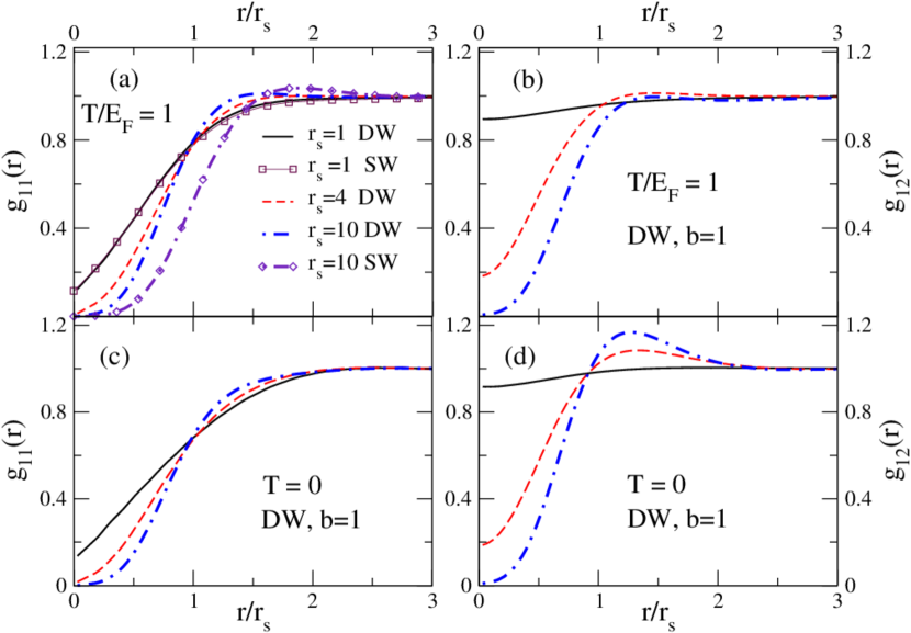
Figure 1: (Color online) Panels (a),(b) show the pair distribution functions $g_{11}(r),g_{12}(r)$ for paramagnetic electrons in a double well (DW) of separation $b=1$, at fixed finite temperature $T/E_{F}=1$, for densities $r_{s}=1,4,10$. The paramagnetic $g_{p}(r)$ for a single well (SW) at $T/E_{F}=1$ is also shown for $r_{s}=1$ and $10$. Panels (c),(d) display the corresponding pair distribution functions at $T=0$ for the double well only.

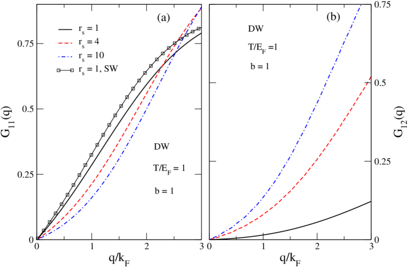
Figure 2: (Color online) (a) The intralayer static local field factors $G_{11}(q)$ for paramagnetic electrons in a double quantum well (DW) of separation $b=1$, at temperature $T/E_{F}=1$ for different densities $r_{s}=1,4,10$. The $G_{11}(q)$ for a single well (SW) at $T/E_{F}=1$ is also shown for $r_{s}=1$. (b) The corresponding interlayer static local field factors $G_{12}(q)$ for the double well only.

The intralayer local field factors $G_{11}(q)=G_{22}(q)$ and the interlayer local field factor $G_{12}(q)$ are determined for the double quantum wells in analogy to Eq. 12, but with the indices now referring to the layers, and using the appropriate diffraction-corrected Coulomb potentials $V^{c}_{ij}(q)$ (see Eqs. II.2 and 16),

$$G_{ij}(q)=\{\tilde{c}_{ij}(q)-c^{0}_{ij}(q)\}/\{\beta_{cf}V^{c}_{ij}(q)\}\ ,$$ (17)

with $\tilde{c}_{ij}(q)=c_{ij}(q)+\beta_{cf}V^{c}_{ij}(q)$.

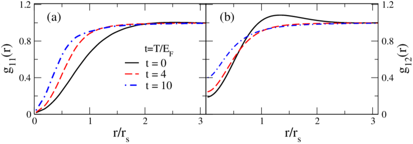
Figure 3: (Color online) The interlayer and intralayer pair distribution functions for paramagnetic electrons in a double quantum well of separation $b=1$, for temperatures $t=T/E_{F}$=0,4,10 at a fixed density $r_{s}=4$.

IV Double quantum wells with carriers of identical charge and mass.

We present results for symmetric double quantum wells containing the same unpolarized carriers at finite temperature $t=T/E_{F}$ and (equal) average interparticle spacings, $r_{s}$, within the layers. Here we take two wells separated by a barrier of width $b=1$ (corresponding to $\sim 5$ nm in graphene and $\sim 10$ nm in GaAs). Finite temperatures can be accessed using Feynman-Path integral methods, and such results would be valuable for bench-marking the CHNC results. However, no calculations are so far available for this system.

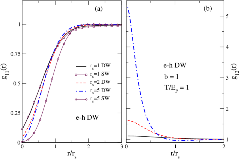
Figure 4: (Color online) Variation of the intralayer and interlayer pair-distribution functions $g_{11}(r)$ and $g_{12}(r)$ at fixed finite temperature $T/E_{F}=1$, for electron-hole quantum double wells (DW) separated by a barrier of thickness $b=1$, for different densities $r_{s}=1,4,5$. Comparison of $g_{11}(r)$ with the $g_{p}(r)$ of a single well (SW) is also given in (a) for $r_{s}=1$ and 5. The value of $\lim_{r\to 0}g_{12}(r)$ increases dramatically with increased coupling (larger $r_{s}$).

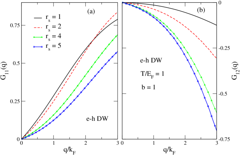
Figure 5: (Color online) The intralayer and interlayer local field factors $G_{11}(q)$ and $G_{12}(q)$ for paramagnetic fluids in electron-hole double quantum wells of separation $b=1$, at fixed finite temperature $T/E_{F}=1$. Results for the densities corresponding to $r_{s}=1,2,4,5$, are displayed. The interlayer local field factor $G_{12}(q)$ becomes negative in the electron-hole system.

In Figs. 1(a) and (c) we display the intralayer pair distribution functions $g_{11}(r)=g_{22}(r)$ for two layers at fixed temperatures $T/E_{F}=1$ and $T=0$, for carrier densities with $r_{s}=1$ to 10. In electrons in GaAs wells, this range corresponds to densities of $n\simeq 3\times 10^{11}$ to $3\times 10^{9}$ cm^-2. For this density range we see that the in-layer pair distribution functions $g_{11}(r)$ are not very sensitive to changes in temperature, at least up to $T/E_{F}=1$.

At the high density $r_{s}=1$, $g_{11}(r)$ for the double quantum well (black line) is almost identical to the paramagnetic $g_{p}(r)$ of a single quantum well (curve marked with boxes). However with decreasing density, as the Coulomb-interaction energy becomes relatively stronger compared to the Fermi energy (e.g., for $r_{s}=10$), we see that the pair distribution functions for the double and single wells are substantially different. The double quantum well pair distribution function $g_{11}(r)$ is less strongly coupled than in a single well, with its maximum at a smaller $r/r_{s}$. For lower densities, the double quantum well $g_{11}(r)$ behaves in a manner similar to $g_{p}(r)$ of a single well at nearly twice the density. This is to be expected at densities for which the average interparticle spacing in a well is much larger than the barrier separation, $r_{s}\gg b$. However, this implies that using local field factors calculated for single wells for use in double well studies, can become a significant source of error for larger $r_{s}$ values.

In Figs. 1(b) and (d) we display the corresponding interlayer pair distribution functions $g_{12}(r)$, which are a measure of the Coulomb correlations between the layers. While the very short-range interlayer correlations are only weakly affected by temperature, at least up to $T/E_{F}=1$ for the density range considered, at larger $r/r_{s}$ the peak found at lower densities in the zero temperature $g_{12}(r)$ that is centered near $r/r_{s}=1.25$, is already completely suppressed by $T/E_{F}=1$. Interestingly, the peak height in $g_{12}(r)$ grows until about $r_{s}\sim 6$, after which it decreases slightly for higher $r_{s}$ values. This is further evidence that, as the Coulomb coupling becomes more important relative to the kinetic energy, the quantum double well behaves increasingly like a single, wider well with larger effective density.

Local field factors at finite $T/E_{F}=1$ are displayed in Figs. 2(a) and (b) for the density range corresponding to $r_{s}=1$ to $10$. The intralayer local field factor $G_{11}(q)$ is only weakly dependent on density, but the interlayer local field factor $G_{12}(q)$, which is small for $r_{s}=1$, grows with decreasing density, and by $r_{s}=10$ it has approached the form of $G_{11}(q)$. This is another indication that the barrier separation, fixed here at $b=1$, has become so small compared with the average interparticle spacing that the separation of the layers no longer affects the correlations. The changes in $G_{12}(q)$ with $r_{s}$ are large by $q=2k_{F}$, which is the important $q$-vector range for the interactions.

Figure 3 shows the pair distribution functions over a wider range of temperatures $t$. The barrier width is again $b=1$. The density is fixed at $r_{s}=4$, corresponding to $n\simeq 2\times 10^{10}$ cm^-2 for electrons in a GaAs well. Both the intralayer and interlayer correlations become weaker with increasing $t$. We saw in Fig. 1 that the zero-temperature peak in $g_{12}(r)$ had already completely disappeared by $t=1$.

V Electron-hole double quantum wells

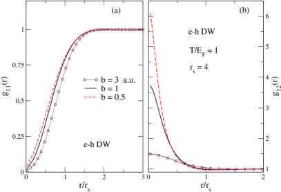
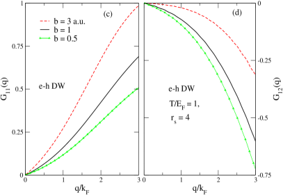
Figure 6: (Color online) (a) The intralayer pair distribution functions for paramagnetic fluids of fixed equal density $r_{s}=4$, in electron-hole double quantum wells at finite temperature $T/E_{F}=1$, for different barrier widths $b$, as labeled. (b) The corresponding interlayer pair distribution functions $g_{12}(r)$. As expected, the value of $g_{12}(r)$ decreases with increasing $b$. (c) The corresponding intralayer local field factors $G_{11}(q)$. (d) The interlayer local field factors $G_{12}(q)$.

Figure 4(a) shows the intralayer pair distribution functions for electron-hole layers at equal densities for fixed finite temperature $T/E_{F}=1$. As already noted, the properties of symmetic double quantum wells are of importance in applications to graphene-like systems where atomically thin (and essentailly equivalent) carrier layers are used. Furthermore, they remain the least challanging candidate for future work using Quantum Monte Carlo and related first principles methods.

In Fig. 4 the barrier thickness is $b=1$. For symmetric wells, $g_{11}(r)=g_{22}(r)$. Figure 4(b) shows the corresponding interlayer pair distribution function $g_{12}(r)$. The value of $\lim_{r\to 0}g_{12}(r)$ increases with increased coupling (increasing $r_{s}$). It should be appreciated that the present theory goes completely beyond the usual mean-field theories that originated with Keldysh Keldysh65 and other early workers (as reviewed in, e.g., Ref. Littlewood1996, ). The CHNC is designed to include XC-effects arising from the interactions beyond mean-field effects. There is of course no provision for excitonic states in the existing CHNC theory although the calculation may remain robust into the weakly bound excitonic regime before it fails. However, the pairing of oppositely charged particles leads to a rearrangement of the ground state of the system. This is accompanied by the appearance of an order parameter proportional to the magnitude of the gap in the single- particle excitation spectrum of the system Lozovik1976a . Since the classical-map technique uses a $T_{q}$ (Eqn. 2) fitted to reproduce the XC-energy of a simple Fermi liquid, the added correlations due to pairing are not included in the present formulation. Since the method is motivated by density-functional ideas (e.g.., uses pair-densities instead of wavefunctions), the possibility of extending the method to regimes of exciton formation, superfluidity etc., may perhaps be envisaged, borrowing ideas from the density-functional approach to phenomena like superconductivity OliveiraGrossKohn88

In Fig. 5 we display the density dependence of the corresponding local field factors for temperature $T/E_{F}=1$. While the intralayer local field factors $G_{11}(q)$ are similar to those of electron-electron double quantum wells, a notable feature here is the negativity of the electron-hole interlayer local field factor $G_{12}(q)$. It is this feature that leads to zeroes in the denominators of response functions, signaling the formation of new elementary excitations, i.e., excitons in this case.

V.1 The effect of the barrier width

The effect of increasing barrier thickness $b$ on the pair distribution functions and the local field factors is presented in Figs. 6 (a) to (d) for an electron-hole double quantum well of fixed equal densities $r_{s}=4$. The barrier width $b$ is varied from $0.5$ to $3$, corresponding in n-GaAs to a range from $5$ nm to $33$ nm. As expected, a thicker barrier weakens the coupling between the layers, so $g_{12}(r)$ and $G_{12}(q)$ are proportionately weakened.

We note the rapid rise of $\lim_{r\to 0}g_{12}(r)$ in Fig. 6(b) as the barrier width is diminished. For density $r_{s}=4$, no convergence was obtained for barrier thickness less than $b\sim 0.267$, at which point $g_{12}(r=0)$ has reached $8.2$. In n-GaAs, $b\sim 0.267$ corresponds to a barrier thickness of $\sim 2.9$ nm. This lack of convergence is a consequence of very strong interactions that cause excitonic bound-states to emerge in the physical system. On general grounds one may expect that if the barrier thickness $b$ were greater than the mean exciton radius, then the system may be relaibaly studied by the present formulation.

VI Conclusions

We have presented results for the pair distribution functions and local field factors as a function of temperature, density and barrier width for electron-electron and electron-hole double quantum wells. While the single-layer CHNC results have been checked against corresponding Quantum Monte Carlo results at $T=0$ to establish its accuracy, comparable QMC results are not yet available at finite-$T$.

Our results confirm that there are significant modifications of the distribution functions and local field factors due to finite-temperature effects, in particular when $T$ exceeds the Fermi temperature. As already noted, in GaAs the Fermi temperature is only $4$ K at a hole layer density $n=4\times 10^{10}$ cm^-2. Our results also reveal that the local field factors calculated for single wells cannot be used for the accurate calculations of properties of double quantum wells, unless the densities are high ($r_{s}\sim 1$).

The local field factors with their density and temperature variation, need to be included in the linear response functions that enter into many measurable properties of double quantum wells. Such properties include (i) thermodynamic functions, (ii) the drag resistivity of interacting double layers as a function of density, temperature and carrier type, (iii) plasmon dispersion in such layers as a function of the density and temperature of the layers, and (iv) energy relaxation of hot electrons injected into one of the layers. The CHNC formalism presented here can be readily generalized to spin polarized layers and to layers with carriers of different effective masses. Our formalism provides high computational efficiency, while providing good to at least modest accuracy in regimes of strong correlations and finite temperatures where other methods become prohibitive.

- (1) Tsuneya Ando, Alan B. Fowler, and Frank Stern, Rev. Mod. Phys. 54, 437 (1982).
- (2) J. Zhu, H. L. Stormer, L. N. Pfeiffer, K. W. Baldwin, and K. W. West, Phys. Rev. Lett. 90, 056805 (2003).
- (3) J. Yoon, C. C. Li, D. Shahar, D. C. Tsui, and M. Shayegan, Phys. Rev. Lett. 82, 1744 (1999).
- (4) L. V. Butov, A. Zrenner, G. Abstreiter, G. Böhm, and G. Weimann, Phys. Rev. Lett. 73, 304 (1994).
- (5) V. B. Timofeev, A. V. Larionov, M. Grassi-Alessi, M. Capizzi, and J. M. Hvam, Phys. Rev. B 61, 8420 (2000).
- (6) J.-P. Cheng, J. Kono, B. D. McCombe, I. Lo, W. C. Mitchel, and C. E. Stutz, Phys. Rev. Lett. 74, 450 (1995)
- (7) J. Kono, B. D. McCombe, J.-P. Cheng, I. Lo, W. C. Mitchel, and C. E. Stutz, Phys. Rev. B 55, 1617 (1997)
- (8) T. P. Marlow, L. J. Cooper, D. D. Arnone, N. K. Patel, D. M. Whittaker, E. H. Linfield, D. A. Ritchie, and M. Pepper, Phys. Rev. Lett. 82, 2362 (1999).
- (9) A. V. Filinov, M. Bonitz, and Yu. E. Lozovik, Physica Status Solidi (c) 0, 1441 (2003).
- (10) A. Perali, D. Neilson, and A. R. Hamilton, Phys. Rev. Letters 110, 146803 (2013).
- (11) L. Świerkowski, D. Neilson, and J. Szymański, Phys. Rev. Lett. 67, 240 (1991).
- (12) M. Zarenia, D. Neilson, and F. M. Peeters, Sci. Rep. 7, 11510 (2017).
- (13) Paweł Jakubczyk, Klaudiusz Majchrowski, and Igor Tralle, Nanoscale Res. Lett. 12, 236 (2017).
- (14) U. Sivan, P. M. Solomon and H. Shtrikman, Phys. Rev. Lett 68, 1196 (1992).
- (15) B. E. Kane, J. P. Eisenstein, W. Wegscheider, L. N. Pfeiffer, K. W West, Appl. Phys. Lett. 65, 3266 (1994).
- (16) J. A. Keogh, K. Das Gupta, H. E. Beere, D. A. Ritchie, and M. Pepper, App. Phys. Lett, 87, 202104 (2005).
- (17) A. F. Croxall, K. Das Gupta, C. A. Nicoll, M. Thangaraj, H. E. Beere, I. Farrer, D. A. Ritchie, and M. Pepper, Phys. Rev. Lett. 101, 246801 (2008).
- (18) J. A. Seamons, C. P. Morath, J. L. Reno, and M. P. Lilly, Phys. Rev. Lett. 102, 026804 (2009).
- (19) B. Zheng, A. F. Croxall, J. Waldie, K. Das Gupta, F. Sfigakis, I. Farrer , H. E. Beere, and D. A. Ritchie, Appl. Phys. Lett. 108, 062102 (2016).
- (20) R. V. Gorbachev, A. K. Geim, M. I. Katsnelson, K. S. Novoselov, T. Tudorovskiy, I. V. Grigorieva, A. H. MacDonald, S. V. Morozov, K.Watanabe, T. Taniguchi, and L. A. Ponomarenko, Nat. Phys. 8, 896 (2012).
- (21) J. I. A. Li, T. Taniguchi, K. Watanabe, J. Hone, A. Levchenko, and C. R. Dean, Phys. Rev. Lett. 117, 046802 (2016).
- (22) Kayoung Lee, Jiamin Xue, David C. Dillen, Kenji Watanabe, Takashi Taniguchi, and Emanuel Tutuc, Phys. Rev. Lett. 117, 046803 (2016).
- (23) G. William Burg, Nitin Prasad, Kyounghwan Kim, Takashi Taniguchi, Kenji Watanabe, Allan H. MacDonald, Leonard F. Register, and Emanuel Tutuc, Phys. Rev. Lett. 120, 177702 (2018).
- (24) L. Świerkowski, J. Szymański, and Z. W. Gortel, Phys. Rev. Lett. 74, 3245 (1995).
- (25) S. De Palo, F. Rapisarda, and G. Senatore, Phys. Rev. Lett. 88, 206401 (2002).
- (26) G. Senatore and S. De Palo, Contrib. Plasma Phys. 43, 363 (2003).
- (27) A. V. Filinov, C. Riva, F. M. Peeters, Yu. E. Lozovik, and M. Bonitz, Phys. Rev. B 70, 035323 (2004).
- (28) R. Maezono, P. López Ríos, T. Ogawa, and R. J. Needs, Phys.Rev. Lett. 110, 216407 (2013).
- (29) Pablo LópezRíos, Andrea Perali, Richard J. Needs, and David Neilson, Phys. Rev. Lett. 120, 177701 (2018).
- (30) Chandre Dharma-wardana A physicist’s view of Matter and Mind, Ch. 8-9 (World Scientific, Singapore, 2014).
- (31) Yu. E. Lozovik and V. I. Yudson, Pis’ma Zh. Eksp. Teor. Fiz. 22, 556 (1975) [JETP Lett. 22, 274 (1975)]
- (32) Yu. E. Lozovik and V. I. Yudson, Solid State Commun. 19, 391 (1976)
- (33) Yu. E. Lozovik and V. I. Yudson, Zh. Eksp. Teor. Fiz. 71, 738 (1976) [Sov. Phys. JETP 44, 389 (1976)].
- (34) Xuejun Zhu, P.B. Littlewood, M. S. Hybertsen, and T. M. Rice, Phys. Rev. Lett 74, 1633 (1995).
- (35) P.B. Littlewood and Xuejun Zhu, Physica Scripta T68, 56 (1996).
- (36) Yu. E. Lozovik and O. L. Berman, Physica Scripta 55, 491 (1997).
- (37) M. Zarenia, A. R. Hamilton, F. M. Peeters, and D. Neilson, Phys. Rev. Lett. 121, 036601 (2018)
- (38) K. S. Singwi, M. P. Tosi, R. H. Land, and A. Sjölander, Phys. Rev. 176 589 (1968);
- (39) M. W. C. Dharma-wardana and F. Perrot, Phys. Rev. Lett. 84, 959 (2000)
- (40) R. B. Laughlin, Phys. Rev. Lett. 50, 1395 (1983).
- (41) F. D. M. Haldane, Phys. Rev. Lett. 51, 605 (1983).
- (42) B. I. Halperin, Phys. Rev. Lett. 52, 1583 (1984).
- (43) A. H. MacDonald, G. C. Aers, and M. W. C. Dharma-wardana, Phys. Rev. B 31, 5529 (1985).
- (44) M. W. C. Dharma-wardanana and F. Perrot, Europhys. Lett. 63, 660 (2003).
- (45) François Perrot and M. W. C. Dharma-wardana, Phys. Rev. Lett. 87, 206404 (2001).
- (46) G. Giuliani and G. Vignale, Quantum theory of the electron liquid (Cambridge Univ. Press, U.K., 2005).
- (47) A.K Rajagopal and J. C. Kimball, Phys. Rev. B 15, 2819 (1977).
- (48) N. Iwamoto, Phys. Rev. A 30, 3289 (1984).
- (49) Juana Moreno and D. C. Marinescu, ArXiv cond-mat/0206465.
- (50) G. S. Atwal, I. G. Khalil and N. W. Ashcroft, Phys. Rev. B 67, 115107 (2003); I. G. Khalil, M. Teter and N. W. Ashcroft, Phys. Rev. B 65, 195309 (2002).
- (51) B. Davoudi, M. Polini, G. F. Giuliani, and M. P. Tosi, Phys. Rev. B 64, 153101 (2001)
- (52) Saverio Moroni, David M. Ceperley, and Gaetano Senatore, Phys. Rev. Lett. 75, 689 (1995).
- (53) François Perrot and M. W. C. Dharma-wardana, Phys. Rev. B 62, 16536 (2000).
- (54) Yu Liu and Jianzhong Wu, J. Chem. Phys 141 064115 (2014)
- (55) M. W. C. Dharma-wardana and F. Perrot, Phys. Rev. Lett. 90, 136601 (2003).
- (56) C. Bulutay and B. Tanatar, Phys. Rev. B 65, 195116 (2002).
- (57) Chieko Totsuji, Takashi Miyake, Kenta Nakanishi, Kenji Tsuruta, and Hiroo Totsuji, J. Phys.: Condens. Matter 21, 045502 (2009).
- (58) M. W. C. Dharma-wardana and F. Perrot, Phys. Rev. B 66, 014110 (2002).
- (59) M. W. C. Dharma-wardana, Proc. Conf. Density Functional Theory, Debrecen, ed. K. Schwarz and A. Nagy, Computation 4 (2), 16 (2016).
- (60) R. Bredow, Th. Bornath, W.-D. Kraeft, M. W. C. Dharma-wardana and R. Redmer, Contrib. Plasma Physics 55, 222 (2015).
- (61) J.Dufty, and S. Dutta, Phys. Rev. E 87, 032101 (2013).
- (62) J. M. J. van Leeuwen, J. Gröneveld, and J. de Boer, Physica 25, 792 (1959).
- (63) Y. Rosenfeld and N. W. Ashcroft, Phys. Rev. A 20, 1208 (1979)
- (64) F. Lado, J. Chem. Phys. 47, 5369 (1967).
- (65) K. Ng, J. Chem. Phys 61, 2680 (1974)
- (66) L. V. Keldysh and Yu. V. Kopaev, Fiz. Tverd. Tela (Leningrad) 6, 2791 (1964) [Sov. Phys. Solid State 6, 2219 (1965)]
- (67) L. N. Oliveira, E. K. U. Gross, and W. Kohn. Phys. Rev. Lett. 60, 2430 (1988)