Angular Parameters Estimation of Multiple Incoherently Distributed Sources Generating Noncircular Signals

Abstract

We introduce a new method for the estimation of the angular parameters [i.e., central directions of arrival (DOAs) and angular spreads] of multiple non-circular and incoherently-distributed (ID) sources and thoroughly analyze its performance. By decoupling the estimation of the central DOAs from that of the angular spreads, we reduce significantly the complexity of the proposed technique. The latter outperforms most well-known state-of-the-art techniques in terms of estimation accuracy and robustness.

Keywords: Angular spread estimation, central DOAs estimation, multiple incoherently distributed sources, noncircular signals, stochastic Cramér-Rao lower bound (CRLB).

I Introduction

Direction of arrivals estimation for multiple plane waves impinging on an arbitrary array of sensors has received a significant amount of attention over the last several decades [References]. It has typically found many applications in different areas such as modern wireless communication systems [References], audio/speech processing systems [References], radar and sonar [References], just to name a few. In most applications, however, DOA estimation methods are based on the point-source model which postulates that the signals are generated from far-field point sources and travel along a single path to the receiving antenna array. Using this simplified model, many DOA estimators have been developed for both temporally uncorrelated [References-References] and correlated [References,References] signals. However, in real-world surroundings, especially in typical urban environments, multipath propagation made by a cluster of reflections close to each mobile causes angular spreading [References]. In other words, the signal radiated by each source hits the antenna array via different paths with different angles. In this more realistic model, the source is viewed by the array as spatially distributed, i.e., with a central DOA and an angular spread. The latter influences the quality of the communication link and represents an important characteristic for spatial diversity schemes [References, References]. DOA estimation becomes more challenging in presence of local scattering [References, References] because the latter affects the signal spatial distribution. In this context, some studies have shown that classical point-source estimation methods suffer from severe performance degradation when applied to the distributed-source scenario [References, References]. This observation has prompted an increasing interest, over the few recent years, in developing DOA estimation algorithms that can handle both point and scattered sources in order to improve direction finding capabilities in real-world propagation environments.
Depending on the nature of scattering, signal components arriving from different directions exhibit varying degrees of correlation. Hence, we distinguish two different types of the propagation channel. The first one is when the received signal components originated from a source and scattered at different angles are delayed and scaled replicas of the same signal. This feature is known in the literature as “coherent source distribution” or “coherently-distributed (CD) source” [References]. The second type of the propagation channel corresponds to the fact that the signal components of a source impinging from different scatterers at different angles are uncorrelated. This is termed in the literature as “incoherent source distribution” or “incoherently-distributed (ID) source” [References, References]. Therefore, for uncorrelated CD sources, each source contributes rank-one component to the spatial covariance matrix and, as such, the rank of the noise-free covariance matrix is equal to the number of sources [References]. Consequently, many classical DOA estimation methods based on the simplistic point-source model can be easily extended to CD sources. Particulary, authors proposed in [References] an efficient DSPE algorithm for estimating the angular parameters of CD sources. This method enables a decoupled estimation of the DOAs from that of the angular spreads of sources with small angular spread. However, for ID sources, the whole observation space is occupied by signal components, and the noise subspace is generally degenerate [References]. Therefore, the rank of the noise-free covariance matrix is different from the number of sources; it even increases with the angular spread. This makes the trivial generalization of traditional point-source subspace-based methods to the ID case not feasible. To sidestep this problem, tremendous efforts have been directed to developing new angular parameters estimators that are specifically tailored to ID sources. In particular, techniques that are able to handle a single ID source were developed in [References-References].
Many estimators were also developed to estimate the angular parameters of multiple ID sources. In fact, a class of subspace methods were proposed in [References, References, References] wherein the effective dimension of the signal subspace is defined as the number of the first eigenvalues (of the noise-free covariance matrix) that reflect most of the signal energy. More computationally attractive approaches that are based on the beamforming techniques were later introduced in [References, References]. Despite their good performance, all these estimators assume the angular distributions to be perfectly known and identical to all the sources. Methods which are able to handle the multi-source case with known but different angular distributions were also proposed in [References, References]. Recently, a robust version of the generalized Capon principle [References] (RGC) has been developed in [References] which, in contrast to all existing approaches, does not need the a priori knowledge of the angular distributions. Moreover, the latter does not need to be the same for all the sources. This robust approach is, however, statistically less efficient than the aforementioned subspace-based (high-resolution) methods [References, References, References], especially in the presence of closely-spaced ID sources.

More recently, A. Zoubir et al. proposed an efficient subspace-based (ESB) algorithm [References] to estimate the angular parameters of multiple ID circular sources. ESB enjoys a good trade-off between estimation performance and computational complexity. In order to alleviate the computational burden stemming from eigendecomposing the covariance matrix, ESB exploits the properties of its inverse and estimates the angular parameters using a 2-D search. Both the statistical efficiency and high-resolution capabilities of the subspace-based techniques are maintained and, most interestingly, ESB is not limited to a particular antenna array geometry or to a specific type of scatterers’ angular distribution. Yet, it still requires the angular distribution to be perfectly known and identical for all the sources on the top of being derived specifically for circular sources. Recently, a new method for tracking the central DOAs assuming multiple ID mobile sources has been also proposed in [References]. It is based on a simple covariance fitting optimization technique [References] to estimate the central DOAs and the Kalman filter to model the dynamic property of directional changes for the moving sources. Despite its efficiency, this method requires the sources’ angular distributions to be perfectly known and is derived for circular sources only.

Noncircular signals, however, such as binary-phase-shift-keying (BPSK) and offset quadrature-phase shift-keying (OQPSK)-modulated signals, are also frequently encountered in digital communications. Therefore, there has been a recent surge of interest in deriving new algorithms that are able to properly handle noncircular signals as well [References-References]. These estimators extract additional information about the angular parameters from the unconjugated spatial covariance matrix that is non-zero for noncircular sources, in contrast to circular ones. From this perspective, we have been also able to propose a robust technique which is able to handle both temporally and spatially correlated sources in presence of noncircular signals [References]. By accounting for both signals’ noncircularity and temporal correlation, the proposed estimator was indeed shown to offer huge performance enhancements with respect to the main state-of-the-art techniques. Yet, all the aforementioned estimators [References-References] are applicable for the point-source model only. And, to the best of the authors’ knowledge, no contribution has dealt so far with the problem of angular parameters estimation (i.e., central DOAs and angular spreads) of multiple noncircular ID sources.

Motivated by these fact, we tackle in this paper for the very first time the problem of estimating the angular parameters of ID noncircular sources. We propose a new method that allows decoupling the estimation of each central DOA from its associated angular spread in the presence of noncircular sources. This method will be derived by going through three different stages resulting in two versions of the proposed estimator. The first one is a new 2-D search algorithm that extends ESB from circular to noncircular sources. And the second is a robust version that estimates the angular parameters by means of two successive one-dimensional (1-D) parameter searches. Towards this goal, we will use unstructured models for the conjugated and unconjugated noise-free covariance matrices that depend on the unknown angular spreads only. Most interestingly, such unstructured models are totally oblivious to the angular distributions of the sources and, therefore, their a priori knowledge is not required by the proposed method; a quite precious degree of freedom in practice. Even more, unlike all the existing methods, the proposed technique does not need to assume the same angular distribution across all the sources.
In order to properly assess the performance of the new estimator, we also conduct a complete theoretical study of its statistical properties (i.e., its bias and variance). Furthermore, we derive an explicit expression for the CRLB of the underlying estimation problem. This fundamental lower bound, which reflects the best achievable performance ever [References], will be used as an overall benchmark against which we gauge the accuracy of the new estimator. Computer simulations will show that the proposed estimator outperforms ESB and RGC especially at low SNR values and/or low DOA separations. The new CRLBs will also reveal that the noncircularity of the signals becomes more informative about the angular parameters when the sources have different angular distributions and when the angular spreads increase.

The rest of this paper is organized as follows. In Section II, we introduce the system model and some of the basic assumptions that will be adopted throughout the article. In section III, we derive the new algorithm and in section IV we show how the estimation of the central DOAs can be decoupled from that of the angular spreads. In section V, we derive the statistical bias and variance of the new estimator. In section VI, we derive an explicit expression for the CRB of the underlying estimation problem. Computer simulations are presented in Section VII and concluding remarks are drawn out in Section VIII.
We list beforehand some of the common notations adopted throughout this paper. Matrices and vectors are represented by bold upper- and lower-case characters, respectively. Vectors are by default in column orientation. Moreover, we consider the following standard notations:

$$\delta(.) : \textrm{Dirac delta function};$$

$$(.)^{*} : \textrm{Complex conjugate};$$

$$\angle(.) : \textrm{Phase angle (or argument) in radians};$$

$$|.| : \textrm{Complex modulus};$$

$$(.)^{T} : \textrm{Transpose};$$

$$(.)^{H} : \textrm{Conjugate transpose};$$

$$\simeq : \textrm{Approximately equal};$$

$$\textrm{argmin}_{K}\{.\} : K$$ Position of the minima of any given

$$\textrm{ objective function};$$

$$\textrm{tr}\{\mathbf{A}\} : \textrm{Trace of a given matrix}~{}\mathbf{A};$$

$$\textrm{diag}\{\bm{v}\} :$$ Diagonal matrix whose main diagonal’s

$$\textrm{elements are those of vector}~{}\bm{v};$$

$$\left\|.\right\|_{\textrm{Fro}} : \textrm{Frobenius norm};$$

$$\Re\{.\} : \textrm{Real part operator};$$

$$\mathbb{E}\{.\} : \textrm{Statistical expectation};$$

$$\frac{\partial^{n}(.)}{\partial(.)^{n}} : \textrm{$n^{th}$-order partial derivative};$$

$$\textrm{eig}\{\mathbf{A}\} : \textrm{Eigenvalues of a matrix}~{}\mathbf{A};$$

$$\varodot : \textrm{Hadamard-Schur product};$$

$$\mathbf{I}_{p} : \textrm{$(p\times p)$ identity matrix};$$

$$\bm{0}_{p\times q} : \textrm{$(p\times q)$ zero matrix};$$

$$\textrm{Toeplitz}\{\bm{v}\} :$$ Symmetric Toeplitz matrix constructed

$$\textrm{from a given vector}~{}\bm{v};$$

$$\textrm{Hankel}\{\bm{v}_{1},\bm{v}_{2}\} :$$ Hankel matrix constructed from the

$$\textrm{vectors}~{}\bm{v}_{1}~{}\textrm{and}~{}\bm{v}_{2};$$

$$a_{l}(\theta) : l$$ Response of the th sensor to a unit-energy

$$\textrm{source radiating from direction}~{}\theta;$$

$${f_{l}(\theta)}_{l=0,2,\ldots,(L-1)} :$$ Real-valued transformations of the scalar

$$\textrm{DOA parameter}~{}\theta;$$

$$\bar{\Theta}_{k} : \textrm{Central DOA of each $k^{th}$ source};$$

$$\bar{\sigma}_{k} : \textrm{Angular spread of each $k^{th}$ source};$$

$$\rho_{k}(\theta,\bar{\bm{\psi}}_{k}) :$$ Normalized angular power density

$$\textrm{of the $k$th source};$$

$$p_{kk}(\theta,\theta^{\prime};\bar{\bm{\psi}}_{k}) :$$ Conjugated angular auto-correlation kernel

$$\textrm{of the $k^{th}$ source};$$

$$p^{\prime}_{kk}(\theta,\theta^{\prime};\bar{\bm{\psi}}_{k}) :$$ Unconjugated angular auto-correlation kernel

$$\textrm{of the $k^{th}$ source};$$

$$p_{kk^{\prime}}(\theta,\theta^{\prime};\bar{\bm{\psi}}_{k},\bar{\bm{\psi}}_{k^{\prime}}) :$$ Conjugated angular cross-correlation kernel

$$\textrm{between sources $k$ and $k^{\prime}$};$$

$$p^{\prime}_{kk^{\prime}}(\theta,\theta^{\prime};\bar{\bm{\psi}}_{k},\bar{\bm{\psi}}_{k^{\prime}}) :$$ Unconjugated angular cross-correlation

$$\textrm{kernel between sources $k$ and $k^{\prime}$}.$$

II System Model

Consider an array consisting of $L$ identical sensors (i.e., with the same gain, phase, and sensitivity pattern) that is immersed in the far-filed of $K$ scattered ID sources with the same central frequency $\omega_{0}$. Assume that the root mean square (rms) delay spread is small compared to the inverse bandwidth of the transmitted signals so that the narrowband assumption remains valid in the presence of scattering [References-References]. Under these mild conditions, the signal received by the $l$th sensor, $l=1,2,\ldots,L$, can be modeled as follows [References-References]:

$$x_{l}(n) = \displaystyle\sum_{k=1}^{K}\int a_{l}(\theta)s_{k}(\theta,\bar{\bm{\psi}}_{k},n)d\theta~{}+~{}w_{l}(n),$$ (1)

in which $n$ stands for the $n$th snapshot. Moreover, $w_{l}(n)$ is an additive zero-mean circularly symmetric Gaussian-distributed noise. The noise components are assumed to be temporally and spatially white, i.e., uncorrelated between snapshots and receiving antenna branches, respectively. Furthermore, $s_{k}(\theta,\bar{\bm{\psi}}_{k},n)$ is the data-modulated angular distribution (with respect to $\theta$) of the signal received from the $k$th source; parameterized here by the vector $\bar{\bm{\psi}}_{k}=[\bar{\Theta}_{k},\bar{\sigma}_{k}]^{T}$.
For any planar configuration of the receiving antenna array, $a_{l}(\theta)$ can be written as:

$$a_{l}(\theta) = e^{j2\pi f_{l-1}(\theta)}.$$ (2)

For mathematical convenience, we gather all the unknown central DOAs and angular spreads in the following parameter vectors:

$$\bar{\bm{\Theta}} \triangleq \left[\bar{\Theta}_{1},\bar{\Theta}_{2},\ldots,\bar{\Theta}_{K}\right]^{T},$$ (3)

$$\bar{\bm{\sigma}} \triangleq \left[\bar{\sigma_{1}},\bar{\sigma_{2}},\ldots,\bar{\sigma}_{K}\right]^{T}.$$ (4)

Our goal in the remainder of this paper is to jointly estimate the angular parameters, $\bar{\bm{\Theta}}$ and $\bar{\bm{\sigma}}$, of the $K$ noncircular sources given the set of received signals, $x_{l}(n)$, $l=1,2,\ldots,L$. To that end, we stack the received data over the $L$ sensors at each snapshot $n$ in a single vector:

$$\mathbf{x}(n) \triangleq [x_{1}(n),\ldots,x_{L}(n)]^{T}.$$ (5)

From (1), $\mathbf{x}(n)$ is explicitly given by:

$$\mathbf{x}(n) = \displaystyle\sum_{k=1}^{K}\int\mathbf{a}(\theta)s_{k}(\theta,\bar{\bm{\psi}}_{k},n)d\theta~{}+~{}\mathbf{w}(n),$$ (6)

where

$$\mathbf{w}(n) \triangleq \left[w_{1}(n),\ldots,w_{L}(n)\right]^{T},$$

$$\mathbf{a}(\theta) \triangleq \left[a_{1}(\theta),\ldots,a_{L}(\theta)\right]^{T},$$

are the array noise and response vectors, respectively. For ID sources, the components impinging from different scatterers are uncorrelated thereby yielding:

$$p_{kk}(\theta,\theta^{\prime};\bar{\bm{\psi}}_{k}) \triangleq \mathbb{E}\Big{\{}s_{k}\big{(}\theta,\bar{\bm{\psi}}_{k},n\big{)}~{}\!s_{k}\big{(}\theta^{\prime},\bar{\bm{\psi}}_{k},n\big{)}^{*}\Big{\}},$$ (7)

$$= \sigma_{s_{k}}^{2}\rho_{k}(\theta,\bar{\bm{\psi}}_{k})\delta(\theta-\theta^{\prime}),$$ (8)

where $\sigma_{s_{k}}^{2}$ is the average power of the $k$th source. Since the sources are also assumed to radiate noncircular signals, we adopt the definition of noncircularity in [References, References]. Moreover, we exploit the property of signals’ correlation in the real sense [References, property $3.1$] to prove from (8) that $p^{\prime}_{kk}(\theta,\theta^{\prime};\bar{\bm{\psi}}_{k})$ can be written as:

$$p^{\prime}_{kk}(\theta,\theta^{\prime};\bar{\bm{\psi}}_{k}) \!\!\!\triangleq\!\!\! \mathbb{E}\Big{\{}s_{k}\big{(}\theta,\bar{\bm{\psi}}_{k},n\big{)}~{}\!s_{k}\big{(}\theta^{\prime},\bar{\bm{\psi}}_{k},n\big{)}\Big{\}},$$ (9)

$$\!\!\!=\!\!\! \sigma_{s_{k}}^{2}\bar{\gamma}_{k}e^{j\bar{\varphi}_{k}}\rho_{k}(\theta,\bar{\bm{\psi}}_{k})\delta(\theta-\theta^{\prime}).$$ (10)

Here, $0\leq\bar{\gamma}_{k}\leq 1$ and $\bar{\varphi}_{k}$ are the noncircularity rate and phase of the $k$th source, respectively. As emphasized in Section II, all existing works on angular parameters estimation of ID sources assume the sources to be circular. As such, none of them makes use of the unconjugated kernels in (9) since they are identically zero in this case. In this paper, however, we consider the case of noncircular sources with maximum noncircularity rate (i.e., $\bar{\gamma}_{k}=1$), known in the open literature as strictly second-order noncircular or rectilinear signals. Examples of such signals include unfiltered BPSK-, OQPSK-, PAM-, ASK-, AM- and MSK-modulated signals [References]. Their unconjugated angular auto-correlation kernels are obtained from (10) as:

$$p^{\prime}_{kk}(\theta,\theta^{\prime};\bar{\bm{\psi}}_{k}) = \sigma_{s_{k}}^{2}e^{j\bar{\varphi}_{k}}\rho_{k}(\theta,\bar{\bm{\psi}}_{k})\delta(\theta-\theta^{\prime}).$$ (11)

Now, since the sources’ signals are uncorrelated from the noise components, the conjugated and unconjugated covariance matrices of $\mathbf{x}(n)$ defined, respectively, as $\mathbf{R}_{\mathbf{x}\mathbf{x}}=\mathbb{E}\{\mathbf{x}(n)\mathbf{x}(n)^{H}\}$ and $\mathbf{R}^{\prime}_{\mathbf{x}\mathbf{x}}=\mathbb{E}\{\mathbf{x}(n)\mathbf{x}(n)^{T}\}$ are explicitly given by:

$$\!\!\mathbf{R}_{\mathbf{x}\mathbf{x}} \!\!\!\!\!=\!\!\!\!\! \displaystyle\sum_{k=1}^{K}\displaystyle\sum_{k^{\prime}=1}^{K}\!\int\!\!\!\!\int p_{kk^{\prime}}(\theta,\theta^{\prime};\bar{\bm{\psi}}_{k},\bar{\bm{\psi}}_{k^{\prime}})\mathbf{a}(\theta)\mathbf{a}^{H}(\theta^{\prime})d\theta d\theta^{\prime}~{}\!\!\!+~{}\!\!\!\sigma_{w}^{2}\mathbf{I}_{L},$$

$$\!\!\mathbf{R}^{\prime}_{\mathbf{x}\mathbf{x}} \!\!\!\!\!\!=\!\!\!\!\!\! \displaystyle\sum_{k=1}^{K}\displaystyle\sum_{k^{\prime}=1}^{K}\!\int\int p^{\prime}_{kk^{\prime}}(\theta,\theta^{\prime};\bar{\bm{\psi}}_{k},\bar{\bm{\psi}}_{k^{\prime}})\mathbf{a}(\theta)\mathbf{a}^{T}(\theta^{\prime})d\theta d\theta^{\prime}\!,$$ (13)

where $\sigma_{w}^{2}$ is the unknown noise variance. Note here that the unconjugated covariance matrix of the circular noise vector is identically zero and, therefore, it vanishes in (13) contrarily to (II). By further assuming the ID sources to be mutually uncorrelated, it follows that:

$$p_{kk^{\prime}}(\theta,\theta^{\prime};\bar{\bm{\psi}}_{k},\bar{\bm{\psi}}_{k^{\prime}}) = p_{kk}(\theta,\theta^{\prime};\bar{\bm{\psi}}_{k},\bar{\bm{\psi}}_{k})\delta_{kk^{\prime}},$$ (14)

$$p^{\prime}_{kk^{\prime}}(\theta,\theta^{\prime};\bar{\bm{\psi}}_{k},\bar{\bm{\psi}}_{k^{\prime}}) = p^{\prime}_{kk}(\theta,\theta^{\prime};\bar{\bm{\psi}}_{k},\bar{\bm{\psi}}_{k})\delta_{kk^{\prime}},$$ (15)

where $\delta_{kk^{\prime}}$ is the Kronecker delta function defined as $\delta_{kk^{\prime}}=1$ for $k=k^{\prime}$ and $0$ otherwise. Now, plugging (8) and (11) in (14) and (15), respectively, leads to:

$$\!\!\!\!p_{kk^{\prime}}(\theta,\theta^{\prime};\bar{\bm{\psi}}_{k},\bar{\bm{\psi}}_{k^{\prime}}) \!\!=\!\! \sigma_{s_{k}}^{2}\rho_{k}(\theta,\bar{\bm{\psi}}_{k})\delta(\theta-\theta^{\prime})\delta_{kk^{\prime}},$$ (16)

$$\!\!\!\!p^{\prime}_{kk^{\prime}}(\theta,\theta^{\prime};\bar{\bm{\psi}}_{k},\bar{\bm{\psi}}_{k^{\prime}}) \!\!=\!\! \sigma_{s_{k}}^{2}e^{j\bar{\varphi}_{k}}\rho_{k}(\theta,\bar{\bm{\psi}}_{k})\delta(\theta-\theta^{\prime})\delta_{kk^{\prime}}.$$ (17)

Consequently, (II) and (13) simplify to:

$$\!\!\!\!\!\!\!\!\!\!\!\mathbf{R}_{\mathbf{x}\mathbf{x}} \!\!=\!\! \displaystyle\sum_{k=1}^{K}\int\sigma_{s_{k}}^{2}\rho_{k}(\theta,\bar{\bm{\psi}}_{k})\mathbf{a}(\theta)\mathbf{a}(\theta)^{H}d\theta~{}+~{}\sigma_{w}^{2}\mathbf{I}_{L},$$ (18)

$$\!\!\!\!\!\!\!\!\!\!\!\mathbf{R}^{\prime}_{\mathbf{x}\mathbf{x}} \!\!=\!\! \displaystyle\sum_{k=1}^{K}\int\sigma_{s_{k}}^{2}e^{j\bar{\varphi}_{k}}\rho_{k}(\theta,\bar{\bm{\psi}}_{k})\mathbf{a}(\theta)\mathbf{a}(\theta)^{T}d\theta.$$ (19)

III Angular Parameters Estimation in Presence of Noncircular Signals

In order to exploit the additional information contained in the unconjugated covariance matrix of noncircular signals, we define the following extended received vector:

$$\widetilde{\mathbf{x}}(n) \triangleq \left[\!\!\begin{array}[]{cc}\mathbf{x}(n)^{T}~{}~{}{\mathbf{x}}(n)^{H}\end{array}\!\!\right]^{T}.$$ (21)

whose extended covariance matrix is given by:

$$\mathbf{R}_{\widetilde{\mathbf{x}}\widetilde{\mathbf{x}}} = \mathbb{E}\Big{\{}\widetilde{\mathbf{x}}(n)\widetilde{\mathbf{x}}(n)^{H}\Big{\}}~{}=~{}\left(\begin{array}[]{cc}\!\!\mathbf{R}_{\mathbf{x}\mathbf{x}}&\mathbf{R}^{\prime}_{\mathbf{x}\mathbf{x}}\!\!\\ \!\!\mathbf{R}^{\prime*}_{\mathbf{x}\mathbf{x}}&\mathbf{R}_{\mathbf{x}\mathbf{x}}^{*}\!\!\end{array}\right).$$ (24)

On the one hand, using the explicit expressions of $\mathbf{R}_{\mathbf{x}\mathbf{x}}$ and $\mathbf{R}^{\prime}_{\mathbf{x}\mathbf{x}}$ established, respectively, in (18) and (19) and resorting to some algebraic manipulations, it can be shown that:

$$\mathbf{R}_{\widetilde{\mathbf{x}}\widetilde{\mathbf{x}}} \!\!\!=\!\!\! \displaystyle\sum_{k=1}^{K}\int\sigma_{s_{k}}^{2}\rho_{k}(\theta,\bar{\bm{\psi}}_{k})~{}\!\widetilde{\mathbf{a}}(\theta,\bar{\varphi}_{k})~{}\!\widetilde{\mathbf{a}}(\theta,\bar{\varphi}_{k})^{H}d\theta~{}+~{}\sigma_{w}^{2}\mathbf{I}_{2L},$$

where $\widetilde{\mathbf{a}}(\theta,\bar{\varphi}_{k})$ is the extended array response vector defined as:

$$\widetilde{\mathbf{a}}(\theta,\bar{\varphi}_{k}) \triangleq \left[\!\!\begin{array}[]{cc}\mathbf{a}(\theta)^{T},~{}~{}e^{-j\bar{\varphi}_{k}}{\mathbf{a}}(\theta)^{H}\end{array}\!\!\right]^{T}.$$ (27)

We also define the extended (normalized) covariance matrix of the noise-free signal pertaining to the $k$th source as:

$$\!\!\!\!\!\!\!\!\widetilde{\mathbf{R}}^{(k)}_{ss}(\bar{\bm{\psi}}_{k},\bar{\varphi}_{k}) \!\triangleq\!\! \int\rho_{k}(\theta,\bar{\bm{\psi}}_{k})\widetilde{\mathbf{a}}(\theta,\bar{\varphi}_{k})\widetilde{\mathbf{a}}(\theta,\bar{\varphi}_{k})^{H}d\theta.$$ (28)

Hence, the extended covariance matrix in (III) is simply given by:

$$\mathbf{R}_{\widetilde{\mathbf{x}}\widetilde{\mathbf{x}}} = \displaystyle\sum_{k=1}^{K}~{}\sigma_{s_{k}}^{2}\widetilde{\mathbf{R}}^{(k)}_{ss}(\bar{\bm{\psi}}_{k},\bar{\varphi}_{k})~{}+~{}\sigma_{w}^{2}\mathbf{I}_{2L}.$$ (29)

Next, we consider the following eigendecomposition of the extended covariance matrix in (29):

$$\mathbf{R}_{\widetilde{\mathbf{x}}\widetilde{\mathbf{x}}} = \widetilde{\mathbf{U}}_{s}\bm{\Sigma}\widetilde{\mathbf{U}}_{s}^{H}~{}+~{}\sigma_{w}^{2}\widetilde{\mathbf{U}}_{w}\widetilde{\mathbf{U}}_{w}^{H},$$ (30)

where $\widetilde{\mathbf{U}}_{s}$ and $\widetilde{\mathbf{U}}_{w}$ denote the eigenvector matrices associated to the signal and noise subspaces, respectively. Moreover, $\bm{\Sigma}$ is a diagonal matrix containing the eigenvalues of the overall extended noise-free covariance matrix involved in (29), i.e.:

$$\mathbf{R}_{\tilde{s}\tilde{s}} \triangleq \sum_{k=1}^{K}\sigma_{s_{k}}^{2}\widetilde{\mathbf{R}}^{(k)}_{ss}(\bar{\bm{\psi}}_{k},\bar{\varphi}_{k}).$$ (31)

Traditional subspace-based methods which are all designed for circular ID sources rely on the fact that the columns of each $k$th noise-free covariance matrix, $\mathbf{R}^{(k)}_{ss}(\bar{\bm{\psi}}_{k})$, are orthogonal to those of the pseudo-noise subspace, i.e.:

$$\mathbf{U}_{w}^{H}~{}\!\mathbf{R}^{(k)}_{ss}(\bar{\bm{\psi}}_{k}) = \bm{0}_{(L-r)\times L},$$ (32)

in which $r$ is the effective dimension of the pseudosignal subspace [References]. In principle, the same orthogonality property in (32) holds for noncircular ID sources:

$$\widetilde{\mathbf{U}}_{w}^{H}\widetilde{\mathbf{R}}^{(k)}_{ss}(\bar{\bm{\psi}}_{k},\bar{\varphi}_{k}) = \bm{0}_{(2L-r)\times 2L},$$ (33)

and can be used, as well, to estimate the associated angular parameters. However, similar to all subspace methods, the estimation performance is critically affected if the effective dimension $r$ is not appropriately selected. Besides, the optimal choice of $r$ depends on the value of the angular spread which is itself considered as an unknown parameter in our work. To sidestep this problem, we will rather capitalize on the inverse of the extended covariance matrix as recently done in [References]:

$$\mathbf{R}_{\widetilde{\mathbf{x}}\widetilde{\mathbf{x}}}^{-1} = \widetilde{\mathbf{U}}_{s}\bm{\Sigma}^{-1}\widetilde{\mathbf{U}}_{s}^{H}~{}+~{}{\frac{1}{\sigma_{w}^{2}}}\widetilde{\mathbf{U}}_{w}\widetilde{\mathbf{U}}_{w}^{H}.$$ (34)

To that end, let $\bm{\psi}$ and $\varphi$ be the two generic variables that run over all the possible values of $\bar{\bm{\psi}}_{k}$ and $\bar{\varphi}_{k}$, respectively. Then, right-multiplying (34) by $\widetilde{\mathbf{R}}^{(k)}_{ss}(\bm{\psi},\varphi)$ yields:

$$\!\!\!\!\!\!\!\!\!\!\!\!\!\mathbf{R}_{\widetilde{\mathbf{x}}\widetilde{\mathbf{x}}}^{-1}\widetilde{\mathbf{R}}^{(k)}_{ss}(\bm{\psi},\varphi) \!\!=\!\! \widetilde{\mathbf{U}}_{s}\bm{\Sigma}^{-1}\widetilde{\mathbf{U}}_{s}^{H}\widetilde{\mathbf{R}}^{(k)}_{ss}(\bm{\psi},\varphi)$$ (35)

$$~{}~{}~{}~{}~{}~{}~{}~{}~{}~{}+~{}{\frac{1}{\sigma_{w}^{2}}}\widetilde{\mathbf{U}}_{w}\widetilde{\mathbf{U}}_{w}^{H}\widetilde{\mathbf{R}}^{(k)}_{ss}(\bm{\psi},\varphi).$$

At relatively high SNR levels, the signal eigenvalues in $\bm{\Sigma}$ are relatively large and, therefore, the diagonal elements of $\bm{\Sigma}^{-1}$ are almost equal to zero. Consequently, the first term in the right-hand side of (35) does not vary appreciably with $\bm{\psi}$ and $\varphi$. The second term in (35) is thus dominant. Owing to (33), however, it is identically zero when $\bm{\psi}=\bar{\bm{\psi}}_{k}$ and $\varphi=\bar{\varphi}_{k}$ (for $k=1,2,\ldots,K$). Therefore, at favorable SNR conditions, the quantity $\|\mathbf{R}_{\widetilde{\mathbf{x}}\widetilde{\mathbf{x}}}^{-1}~{}\!\widetilde{\mathbf{R}}^{(k)}_{ss}(\bm{\psi},\varphi)\|_{\textrm{Fro}}$ attains its minimum at $(\bar{\bm{\psi}}_{k},~{}\bar{\varphi}_{k})$ for each $k=1,2,\ldots,K$. Based on this observation, the angular parameters can be estimated jointly with the sources’ noncircularity phases by resolving the following $K$ optimization problems:

$$\!\!\!\!\!\!\!\!\!\!\left[\widehat{\bar{\bm{\psi}}}_{k},~{}\!\widehat{\bar{\varphi}}_{k}\right] \!\!\!=\!\!\! \underset{\bm{\psi},\bm{\varphi}}{\operatorname{argmin}}\left(\left\|\widehat{\mathbf{R}}_{\widetilde{\mathbf{x}}\widetilde{\mathbf{x}}}^{-1}\widetilde{\mathbf{R}}^{(k)}_{ss}(\bm{\psi},\varphi)\right\|_{\textrm{Fro}}^{2}\right)\!,$$ (36)

$$\!\!\!=\!\!\! \underset{\bm{\psi},\bm{\varphi}}{\operatorname{argmin}}\left(\textrm{tr}\Big{\{}\widetilde{\mathbf{R}}^{(k)}_{ss}(\bm{\psi},\varphi)~{}\!\widehat{\mathbf{R}}_{\widetilde{\mathbf{x}}\widetilde{\mathbf{x}}}^{-2}~{}\widetilde{\mathbf{R}}^{(k)}_{ss}(\bm{\psi},\varphi)\Big{\}}\right)\!,$$ (37)

where $\widehat{\mathbf{R}}_{\widetilde{\mathbf{x}}\widetilde{\mathbf{x}}}$ is the sample-mean estimate of the actual extended covariance matrix, $\mathbf{R}_{\widetilde{\mathbf{x}}\widetilde{\mathbf{x}}}$, i.e.:

$$\widehat{\mathbf{R}}_{\widetilde{\mathbf{x}}\widetilde{\mathbf{x}}}~{}=~{}\frac{1}{N}\sum_{n=1}^{N}\widetilde{\mathbf{x}}(n)\widetilde{\mathbf{x}}(n)^{H},$$ (38)

in which $N$ stands for the number of snapshots. Further, if the sources have the same scatterers’ angular distribution [i.e., $\widetilde{\mathbf{R}}^{(k)}_{ss}(\bm{\psi},\varphi)=\widetilde{\mathbf{R}}_{ss}(\bm{\psi},\varphi)$, $\forall k$], then all the angular parameters can be estimated jointly by finding the location of the $K$ smallest values of the common cost function:

$$~{}\!\!\!f\big{(}\bm{\psi},\varphi\!~{}\big{|}\!~{}\widehat{\mathbf{R}}_{\widetilde{\mathbf{x}}\widetilde{\mathbf{x}}}^{-2}\big{)} \triangleq \textrm{tr}\Big{\{}\widetilde{\mathbf{R}}_{ss}(\bm{\psi},\varphi)~{}\!\widehat{\mathbf{R}}_{\widetilde{\mathbf{x}}\widetilde{\mathbf{x}}}^{-2}~{}\widetilde{\mathbf{R}}_{ss}(\bm{\psi},\varphi)\Big{\}},$$ (39)

where

$$\!\!\widetilde{\mathbf{R}}_{ss}(\bm{\psi},\varphi) = \int\rho(\theta,\bm{\psi})~{}\!\widetilde{\mathbf{a}}(\theta,\varphi)~{}\!\widetilde{\mathbf{a}}(\theta,\varphi)^{H}d\theta.$$ (40)

Note here that the cost function in (39) to be minimized requires a three-dimensional (3-D) search over the central DOA, $\Theta$, the angular spread, $\sigma$, and the noncircularity phase, $\varphi$. In the following, we will try to reduce the complexity of the proposed method by reducing the dimensionality of the cost function in (39).

Actually, using (27) in (40), it can be shown that:

$$\!\!\widetilde{\mathbf{R}}_{ss}(\bm{\psi},\varphi) = \left(\begin{array}[]{cc}\mathbf{R}_{ss}(\bm{\psi})&e^{j\varphi}\mathbf{R}^{\prime}_{ss}(\bm{\psi})\\ {}\hfil\\ e^{-j\varphi}\mathbf{R}^{\prime*}_{ss}(\bm{\psi})&\mathbf{R}_{ss}^{*}(\bm{\psi})\end{array}\right),$$ (44)

where $\mathbf{R}_{ss}(\bm{\psi})$ and $\mathbf{R}^{\prime}_{ss}(\bm{\psi})$ are, respectively, the normalized conjugated and unconjugated noise-free auto-covariance matrices of the sources which are explicitly given by:

$$\mathbf{R}_{ss}(\bm{\psi}) = \int\rho(\theta,\bm{\psi})\mathbf{a}(\theta)\mathbf{a}(\theta)^{H}d\theta,$$ (45)

$$\mathbf{R}^{\prime}_{ss}(\bm{\psi}) = \int\rho(\theta,\bm{\psi})\mathbf{a}(\theta)\mathbf{a}(\theta)^{T}d\theta.$$ (46)

Assuming small angular spreads, we prove in Appendix A that $\mathbf{R}_{ss}(\bar{\bm{\psi}}_{k})$ can be written for each $k$th source as:

$$\!\!\!\!\!\!\!\!\mathbf{R}_{ss}(\bar{\bm{\psi}}_{k}) \simeq \Big{(}\mathbf{a}(\bar{\Theta}_{k})\!~{}\mathbf{a}(\bar{\Theta}_{k})^{H}\Big{)}\varodot\mathbf{T}(\bar{\bm{\psi}}_{k})$$ (47)

$$\simeq \bm{\Phi}(\bar{\Theta}_{k})\!~{}\mathbf{T}(\bar{\bm{\psi}}_{k})\!~{}\bm{\Phi}(\bar{\Theta}_{k})^{H},$$

with $\bm{\Phi}(\bar{\Theta}_{k})~{}\triangleq~{}\textrm{diag}\{\mathbf{a}(\bar{\Theta}_{k})\}$ and $\mathbf{T}(\bar{\bm{\psi}}_{k})$ is a real-valued $(L\times L)$ symmetric matrix whose $(p,l)$th entry is given by:

$$[\mathbf{T}]_{pl}(\bar{\bm{\psi}}_{k}) \!\!\!\!\!\!=\!\!\!\!\!\!\!\! \int\!\!\!\rho_{k}(\theta,\bar{\bm{\psi}}_{k})\!\cos\!\bigg{(}\!2\pi\!\left(f^{\prime}_{p-1}(\bar{\Theta}_{k})\!-\!f^{\prime}_{l-1}(\bar{\Theta}_{k})\right)\!(\theta\!-\!\bar{\Theta}_{k})\!\bigg{)}\!d\theta,$$

and $f^{\prime}_{p-1}(\theta)$ stands for the first derivative of $f_{p-1}(\theta)$ with respect to $\theta$.
In the same way, we also show that the normalized unconjugated noise-free covariance matrix, $\mathbf{R}^{\prime}_{ss}(\bar{\bm{\psi}}_{k})$, of noncircular ID sources can be be expressed as:

$$\mathbf{R}^{\prime}_{ss}(\bar{\bm{\psi}}_{k}) \!\!\!\simeq\!\!\! \Big{(}\mathbf{a}(\bar{\Theta}_{k})\!~{}\mathbf{a}(\bar{\Theta}_{k})^{T}\Big{)}\varodot\mathbf{T}^{\prime}(\bar{\bm{\psi}}_{k})$$ (49)

$$\simeq \bm{\Phi}(\bar{\Theta}_{k})\!~{}\mathbf{T}^{\prime}(\bar{\bm{\psi}}_{k})\!~{}\bm{\Phi}(\bar{\Theta}_{k})^{T},$$

where $\mathbf{T}^{\prime}(\bar{\bm{\psi}}_{k})$ is also a real-valued $(L\times L)$ symmetric matrix whose $(p,l)$th entry is given by:

$$[\mathbf{T}^{\prime}]_{pl}(\bar{\bm{\psi}}_{k}) \!\!\!\!\!\!=\!\!\!\!\!\!\!\! \int\!\!\!\rho_{k}(\theta,\bar{\bm{\psi}}_{k})\!\cos\!\bigg{(}\!2\pi\!\left(f^{\prime}_{p-1}(\bar{\Theta}_{k})\!+\!f^{\prime}_{l-1}(\bar{\Theta}_{k})\right)\!(\theta\!-\!\bar{\Theta}_{k})\!\bigg{)}\!d\theta.$$

Injecting (47) and (49) back into (44) with the generic $\bm{\psi}$ and $\Theta$ being substituted for $\bar{\bm{\psi}}_{k}$ and $\bar{\Theta}_{k}$, respectively, and resorting to some straightforward manipulations, it can be shown that:

$$\widetilde{\mathbf{R}}_{ss}(\bm{\psi},\varphi) \!\!=\!\! \Big{(}\widetilde{\mathbf{a}}(\Theta,\varphi)\!~{}\widetilde{\mathbf{a}}(\Theta,\varphi)^{H}\Big{)}\varodot\widetilde{\mathbf{T}}(\bm{\psi}),$$ (51)

$$\!\!=\!\! \widetilde{\bm{\Phi}}(\Theta,\varphi)~{}\!\widetilde{\mathbf{T}}(\bm{\psi})~{}\!\widetilde{\bm{\Phi}}(\Theta,\varphi)^{H},$$

in which $\widetilde{\bm{\Phi}}(\Theta,\varphi)~{}=~{}\textrm{diag}\{\widetilde{\mathbf{a}}(\Theta,\varphi)\}$ and

$$\widetilde{\mathbf{T}}(\bm{\psi}) = \left(\begin{array}[]{cc}\mathbf{T}(\bm{\psi})&~{}~{}{\mathbf{T}^{\prime}}(\bm{\psi})\\ \\ {\mathbf{T}^{\prime}}(\bm{\psi})&~{}~{}\mathbf{T}(\bm{\psi})\end{array}\right).$$ (55)

For mathematical convenience, we also introduce the following notations:

$$\mathbf{A}(\bm{\psi}) \!\!=\!\! \mathbf{T}^{2}(\bm{\psi})+{\mathbf{T}^{\prime}}^{2}(\bm{\psi}),$$ (56)

$$\mathbf{B}(\bm{\psi}) \!\!=\!\! \mathbf{T}(\bm{\psi}){\mathbf{T}^{\prime}}(\bm{\psi})+{\mathbf{T}^{\prime}}(\bm{\psi})\mathbf{T}(\bm{\psi}),$$ (57)

$$\widehat{\mathbf{R}}_{1} \!\!=\!\! \widehat{\mathbf{R}}_{\widetilde{\mathbf{x}}\widetilde{\mathbf{x}}}^{-2}(1:L,1:L),$$ (58)

$$\widehat{\mathbf{R}}_{2} \!\!=\!\! \widehat{\mathbf{R}}_{\widetilde{\mathbf{x}}\widetilde{\mathbf{x}}}^{-2}(1:L,L+1:2L).$$ (59)

Then, plugging (51) back into (39), we prove after tedious manipulations (cf. Appendix B), that the angular parameters, $\{\bar{\bm{\psi}}_{k}\}_{k=1}^{K}$, can now be estimated by minimizing the following compressed cost function (i.e., that depends on $\bm{\psi}$ only):

$$\!\!\!\!\!\!\!\!\!\!\!\!f_{c}\big{(}\bm{\psi}\!~{}\big{|}\!~{}\widehat{\mathbf{R}}_{\widetilde{\mathbf{x}}\widetilde{\mathbf{x}}}^{-2}\big{)}$$ (60)

$$\!\!\!\!\!\!\!\!\!\!\!\!\!\!\!\!\!\!\!\!\!\!\!\!=~{}\!\Re\bigg{\{}\textrm{tr}\Big{\{}\textrm{diag}\big{\{}\mathbf{a}(\Theta)\big{\}}\mathbf{A}(\bm{\psi})\textrm{diag}\big{\{}\mathbf{a}(\Theta)^{H}\big{\}}\widehat{\mathbf{R}}_{1}\Big{\}}\bigg{\}}$$

$$\!\!\!\!\!\!-\bigg{|}~{}\!\textrm{tr}\Big{\{}\textrm{diag}\big{\{}\mathbf{a}(\Theta)\big{\}}\mathbf{B}(\bm{\psi})\textrm{diag}\big{\{}\mathbf{a}(\Theta)\big{\}}^{T}\widehat{\mathbf{R}}_{2}^{*}\Big{\}}\bigg{|}.$$

Note here that the first version of our proposed method defined by the cost function in (60) is applicable for a general class of angular distributions (symmetric distributions with small angular spreads) and any planar array configuration. However, it requires the a priori knowledge of the angular distributions to calculate the matrices $\mathbf{A}$ and $\mathbf{B}$ from (56) and (57), respectively. Furthermore, finding the $K$ minima of (60) with respect to $\bm{\psi}=\big{[}\Theta,~{}\sigma\big{]}^{T}$ still requires a two-dimensional (2-D) search over $\Theta$ and $\sigma$ and needs the angular distribution to be identical for all the sources to estimate jointly the angular parameters. In the following, we will build upon some properties of the matrices $\mathbf{T}(\bm{\psi})$ and ${\mathbf{T}^{\prime}}(\bm{\psi})$ in order to decouple the estimation of the central DOAs from that of the angular spreads [References]. These properties are valid for any symmetric source’s angular distribution with small angular spreads. Hence, the estimator can be implemented by two successive one-dimensional (1-D) parameter searches, thereby resulting in tremendous computational savings. Moreover, we will exploit these properties to establish unstructured models for $\mathbf{T}(\bm{\psi})$ and ${\mathbf{T}^{\prime}}(\bm{\psi})$ that are totally oblivious to the symmetric sources’ angular distributions. Therefore, we will obtain a new version of the proposed estimator that does not require the a priori knowledge of the sources’ angular distributions.

IV Robust Version of the Proposed Estimator

To begin with, for any array configuration, recall that $\mathbf{T}(\bm{\psi})$ is a real-valued symmetric matrix whose expression is given by (III). Moreover, we prove in the following that if $f^{\prime}_{p-1}(\bar{\Theta}_{k})$ is expressed as follows:

$$f^{\prime}_{p-1}(\bar{\Theta}_{k}) = (p-1)g(\bar{\Theta}_{k}),$$ (61)

where $g(\bar{\Theta}_{k})$ is a transformation of the central DOA $\bar{\Theta}_{k}$, then $\mathbf{T}(\bar{\bm{\psi}}_{k})$ is a symmetric Toeplitz matrix. In fact, injecting (61) in (III), we show that $[\mathbf{T}]_{pl}(\bar{\bm{\psi}}_{k})$ can be written as follows:

$$\!\!\!\![\mathbf{T}]_{pl}(\bar{\bm{\psi}}_{k}) \!\!\!\!\!\!=\!\!\!\!\!\! \int\!\rho_{k}(\theta,\bar{\bm{\psi}}_{k})\cos\left(2\pi(p-l)g(\bar{\Theta}_{k})\!(\theta\!-\!\bar{\Theta}_{k})\right)\!d\theta.$$ (62)

From (62), we can simply verify that:

$$[\mathbf{T}]_{pl}(\bar{\bm{\psi}}_{k}) \!\!\!=\!\!\! [\mathbf{T}]_{(p+m)(l+m)}(\bar{\bm{\psi}}_{k}),\forall m.$$ (63)

Consequently, $\mathbf{T}(\bar{\bm{\psi}}_{k})$ is a symmetric Toeplitz matrix and, therefore, it can be fully constructed from its first column vector denoted here as $\mathbf{t}_{1}$, i.e.:

$$\mathbf{T}(\bm{\psi}) = \textrm{Toeplitz}\big{(}\mathbf{t}_{1}\big{)}.$$ (64)

Moreover, for any symmetric angular distribution, we prove in Appendix C that if its angular spread verifies the following condition:

$$\sigma<\frac{1}{\sqrt{2}\pi(L-1)g(\bar{\Theta}_{k})},$$ (65)

then the elements, $\{\mathbf{t}_{1}(l)\}_{l=1}^{L}$, of the vector, $\mathbf{t}_{1}$, satisfy the following property:

$$1~{}=~{}\mathbf{t}_{1}(1)~{}\geq~{}\mathbf{t}_{1}(2)~{}\geq\ldots\geq~{}\mathbf{t}_{1}(L)~{}\geq~{}0.$$ (66)

(65) is a nonrestrictive condition for propagation environments characterized by small angular spreads, e.g., macro-cell environments [References-References]. Actually, (66) can be rewritten in the more succinct form:

$$\mathbf{J}_{L}\mathbf{t}_{1}~{}\leq~{}\mathbf{e}_{L},$$ (67)

where $\mathbf{J}_{n}$ is from now on a ($n\times n$) matrix given by:

$$\mathbf{J}_{n} = \left(\begin{array}[]{ccccc}1&0&0&\cdots&0\\ -1&1&0&\cdots&0\\ 0&-1&1&\ddots&0\\ \vdots&\ddots&\ddots&\ddots&\vdots\\ 0&\cdots&\cdots&-1&1\\ 0&\cdots&\cdots&0&-1\end{array}\right),$$ (74)

and $\mathbf{e}_{n}$ is a $n-$dimensional vector given by $\mathbf{e}_{n}=[1,0,\ldots,0]^{T}$.
For any array configuration, recall also that ${\mathbf{T}^{\prime}}(\bm{\psi})$ is a real-valued symmetric matrix whose expression is given by (III). Moreover, if $f^{\prime}_{p-1}(\bar{\Theta}_{k})$ satisfies (61), we show that $[\mathbf{T}^{\prime}]_{pl}(\bar{\bm{\psi}}_{k})$ can be written as:

$$\!\!\!\!\!\!\!\!\!\![\mathbf{T}^{\prime}]_{pl}(\bar{\bm{\psi}}_{k}) \!\!\!\!\!\!=\!\!\!\!\!\!\!\! \int\!\!\rho_{k}(\theta,\bar{\bm{\psi}}_{k})\cos\!\left(2\pi(p+l-2)g(\bar{\Theta}_{k})\!(\theta\!-\!\bar{\Theta}_{k})\right)\!d\theta.$$ (75)

From (75), we can see that ${\mathbf{T}^{\prime}}(\bm{\psi})$ is a Hankel matrix. Therefore, it can be constructed from its first and last column vectors denoted, respectively, as $\mathbf{t}^{\prime}_{1}$ and $\mathbf{t}^{\prime}_{L}$ as follows:

$$\mathbf{T}^{\prime}(\bm{\psi}) = \textrm{Hankel}\big{(}\mathbf{t}^{\prime}_{1},\mathbf{t}^{\prime}_{L}\big{)}.$$ (76)

Moreover, for any symmetric source’s angular distribution, we also prove in Appendix C that if $\sigma<1/\big{(}2\sqrt{2}\pi(L-1)g(\bar{\Theta}_{k})\big{)}$, then the elements of $\mathbf{t}^{\prime}_{1}$ and $\mathbf{t}^{\prime}_{L}$ satisfy the following properties:

$$\mathbf{J}_{L}\mathbf{t}^{\prime}_{1}\leq\mathbf{e}_{L},~{}~{}~{}\mathbf{J}_{L}\mathbf{t}^{\prime}_{L}\leq\mathbf{e}_{L},~{}~{}~{}\textrm{and}~{}~{}~{}\mathbf{t}^{\prime}_{1}(L)=\mathbf{t}^{\prime}_{L}(1).$$ (77)

Furthermore, we verify that the first column vector of ${\mathbf{T}^{\prime}}(\bm{\psi})$ is identical to the first column vector of $\mathbf{T}(\bm{\psi})$, i.e., we have the following relation:

$$\mathbf{t}_{1} = \mathbf{t}^{\prime}_{1}.$$ (78)

In order to exploit the interesting properties stated above in (67), (77) and (78), we consider an auxiliary vector $\mathbf{z}=[z_{1},\ldots,z_{L-1},z_{L},\ldots,z_{2L-2}]^{T}$ whose elements are all in $[0,1]$ and sorted in decreasing order:

$$1\geq z_{1}\geq z_{2}\geq\ldots\geq z_{L-1}\geq z_{L}\geq\ldots\geq z_{2L-2}\geq 0,$$ (79)

or equivalently:

$$\mathbf{J}_{2L-1}\mathbf{z}\leq\mathbf{e}_{2L-1}.$$ (80)

Then, we construct the following two auxiliary matrices:

$$\mathbf{Z} \!\!=\!\! \textrm{Toeplitz}\Big{(}\big{[}1,\mathbf{z}(1:L-1)\big{]}\Big{)},$$ (81)

$$\mathbf{Z}^{\prime} \!\!=\!\! \textrm{Hankel}\Big{(}\big{[}1,\mathbf{z}(1:L-1)\big{]},\mathbf{z}(L-1:2L-2)\Big{)},$$ (82)

which also verify the constraints in (67) and (77), respectively. Therefore, bearing in mind the expressions of the matrices $\mathbf{A}$ and $\mathbf{B}$ in (56) and (57), respectively, it follows that instead of minimizing the 2-D criterion in (60), one can start by solving the following 1-D constrained optimization problem in order to find the central DOAs:

$$\!\!\!\!\!\!\!\!\!\widehat{\bar{\bm{\Theta}}} \!\!=\!\! \arg\underset{\Theta}{{\min}_{K}}\bigg{(}\underset{\mathbf{z}}{\min}~{}g(\Theta,\mathbf{z})~{}~{}~{}~{}\textrm{subject to}~{}~{}~{}~{}(\ref{consminprobopt})\bigg{)},$$ (83)

where

$$\!\!\!\!g(\Theta,\mathbf{z}) \!\!\!=\!\!\! \Re\Bigg{\{}\textrm{tr}\bigg{\{}\textrm{diag}\big{\{}\mathbf{a}(\Theta)\big{\}}\big{(}\mathbf{Z}^{2}+\mathbf{Z}^{\prime 2}\big{)}\textrm{diag}\big{\{}\mathbf{a}(\Theta)^{H}\big{\}}\widehat{\mathbf{R}}_{1}\bigg{\}}\Bigg{\}}$$

$$-~{}~{}\Bigg{|}~{}\!\textrm{tr}\bigg{\{}\textrm{diag}\big{\{}\mathbf{a}(\Theta)\big{\}}\big{(}\mathbf{Z}\mathbf{Z}^{\prime}+\mathbf{Z}^{\prime}\mathbf{Z}\big{)}\textrm{diag}\big{\{}\mathbf{a}(\Theta)^{T}\big{\}}\widehat{\mathbf{R}}_{2}^{*}\bigg{\}}\Bigg{|}.$$

The optimization task in (83) can be solved efficiently via the well-known sequential quadratic programming (SQP) algorithm which is a rapidly converging descent method for nonlinearly-constrained optimization problems [References]. Interestingly enough, the estimator in (83) is also totally oblivious to the sources’ angular distributions provided that the latter be symmetric. In fact, the auxiliary matrices $\mathbf{Z}$ and $\mathbf{Z}^{\prime}$ involved in (80) were built for any symmetric angular distribution upon some general properties shared by $\mathbf{T}$ and $\mathbf{T}^{\prime}$, respectively, and not their true expressions as required in (60). Moreover, this estimator is applicable in the more challenging scenario where the sources have different angular distributions. These are actually quite precious degrees of freedom in practice since the angular distribution may vary from one environment to another and/or from source to source in real-world scenarios. After acquiring the central DOAs, $\widehat{\bar{\mathbf{\Theta}}}\!~{}=~{}\!\big{[}\widehat{\bar{\Theta}}_{1},\widehat{\bar{\Theta}}_{2},\ldots,\widehat{\bar{\Theta}}_{K}\big{]}$, as in (83), the angular spread pertaining to each $k$th source is estimated as follows:

$$\!\!\!\widehat{\bar{\sigma}}_{k} = \arg\underset{\sigma}{\min}~{}f_{c}\big{(}\widehat{\bar{\Theta}}_{k},\sigma\!~{}\big{|}\!~{}\widehat{\mathbf{R}}_{\widetilde{\mathbf{x}}\widetilde{\mathbf{x}}}^{-2}\big{)},$$ (85)

where $f_{c}(.)$ is the compressed cost function already established in (60). Our estimator actually reduces to (83) and (85), that is after going through three different derivation stages, from (39) to (60), ultimately leading to our final robust solution.

V Statistical Properties

In order to assess the theoretical performance limits of the proposed estimator, we will express its mean square error (MSE) analytically, based on the minimization of the original cost function, $f\big{(}\bm{\psi},\varphi~{}\!\big{|}\!~{}\widehat{\mathbf{R}}_{\widetilde{\mathbf{x}}\widetilde{\mathbf{x}}}^{-2}\big{)}$, given in (39) instead of the compressed one in (60) due to the presence of the nonlinear modulus operator in it. We will also use $\bm{\alpha}_{k}=[\bar{\bm{\psi}}^{T}_{k},\bar{\varphi}_{k}]^{T}=[\bar{\Theta}_{k},\bar{\sigma}_{k},\bar{\varphi}_{k}]^{T}$ to denote the entire unknown parameter vector pertaining to each $k$th noncircular ID source. We further use:

$$\mathbf{b}(\widehat{\bm{\alpha}}_{k}) \triangleq \mathbb{E}\{\widehat{\bm{\alpha}}_{k}\}~{}-~{}\bm{\alpha}_{k},$$ (86)

$$\mathbf{V}(\widehat{\bm{\alpha}}_{k}) \triangleq \mathbb{E}\Big{\{}\big{(}\widehat{\bm{\alpha}}_{k}-\mathbb{E}\{\widehat{\bm{\alpha}}_{k}\}\big{)}\big{(}\widehat{\bm{\alpha}}_{k}-\mathbb{E}\{\widehat{\bm{\alpha}}_{k}\}\big{)}^{T}\Big{\}},$$ (87)

to denote, respectively, the bias vector and covariance matrix of the estimate $\widehat{\bm{\alpha}}_{k}$. To begin with, it is easy to show that the mean square error (MSE), defined as $\textrm{MSE}(\widehat{\bm{\alpha}}_{k})\triangleq\mathbb{E}\big{\{}(\widehat{\bm{\alpha}}_{k}-\bm{\alpha}_{k})(\widehat{\bm{\alpha}}_{k}-\bm{\alpha}_{k})^{T}\big{\}}$, is given by:

$$\textrm{MSE}(\widehat{\bm{\alpha}}_{k}) = \mathbf{b}(\widehat{\bm{\alpha}}_{k})\mathbf{b}^{T}(\widehat{\bm{\alpha}}_{k})~{}+~{}\mathbf{V}(\widehat{\bm{\alpha}}_{k}).$$ (88)

Moreover, similar to [References], let $\breve{\bm{\alpha}}_{k}$ denote the asymptotic estimate (obtained when the number of snapshots $N\rightarrow\infty$), and define $\Delta\bm{\alpha}_{k}~{}\triangleq~{}\breve{\bm{\alpha}}_{k}~{}-~{}\bm{\alpha}_{k}$ and $\Delta\breve{\bm{\alpha}}_{k}~{}\triangleq~{}\widehat{\bm{\alpha}}_{k}-\breve{\bm{\alpha}}_{k}$. Then, it immediately follows from (86) that $\mathbf{b}(\widehat{\bm{\alpha}}_{k})$ decomposes as the sum of the asymptotic bias and the residual bias stemming from the finite-sample effects:

$$\mathbf{b}(\widehat{\bm{\alpha}}_{k}) = \mathbb{E}\{\Delta\bm{\alpha}_{k}\}~{}+~{}\mathbb{E}\{\Delta\breve{\bm{\alpha}}_{k}\}.$$ (89)

Furthermore, using some relatively straightforward algebraic manipulations, it can be shown that:

$$\mathbf{V}(\widehat{\bm{\alpha}}_{k}) = \mathbb{E}\big{\{}\Delta\breve{\bm{\alpha}}_{k}\Delta\breve{\bm{\alpha}}^{T}_{k}\big{\}}~{}-~{}\mathbb{E}\big{\{}\Delta\breve{\bm{\alpha}}_{k}\big{\}}\mathbb{E}\big{\{}\Delta\breve{\bm{\alpha}}^{T}_{k}\big{\}}.$$ (90)

Plugging (89) and (90) back into (88), it follows that:

$$\!\!\!\!\!\!\!\!\!\!\!\!\!\!\!\!\textrm{MSE}(\widehat{\bm{\alpha}}_{k}) \!\!=\!\! \mathbb{E}\big{\{}\Delta\bm{\alpha}_{k}\Delta\bm{\alpha}^{T}_{k}\big{\}}~{}\!+~{}\!\mathbb{E}\big{\{}\Delta\bm{\alpha}_{k}\big{\}}\mathbb{E}\big{\{}\Delta\breve{\bm{\alpha}}_{k}\big{\}}^{T}$$ (91)

$$~{}~{}~{}+~{}\!\mathbb{E}\big{\{}\Delta\breve{\bm{\alpha}}_{k}\big{\}}\mathbb{E}\big{\{}\Delta\bm{\alpha}_{k}\big{\}}^{T}+\mathbb{E}\big{\{}\Delta\breve{\bm{\alpha}}_{k}\Delta\breve{\bm{\alpha}}^{T}_{k}\big{\}}\!.$$

In order to establish an analytical expression for $\textrm{MSE}(\hat{\bm{\alpha}}_{k})$, we will derive hereafter the four expectations involved in (91) separately. To do so, we use $\bm{\alpha}$ and $\mathbf{R}$ as generic variables for $\bm{\alpha}_{k}$ and $\widehat{\mathbf{R}}^{-2}_{\widetilde{\mathbf{x}}\widetilde{\mathbf{x}}}$, respectively. We also denote the gradient vector and Hessian matrix of the scalar-valued objective function, $f(\bm{\alpha},\mathbf{R})$, as follows:

$$\mathbf{f}(\bm{\alpha}|\mathbf{R}) \triangleq \frac{\partial f(\bm{\alpha}|\mathbf{R})}{\partial\bm{\alpha}},~{}~{}~{}~{}~{}~{}~{}~{}\textrm{(gradient vector)}$$

$$\mathbf{F}(\bm{\alpha}|\mathbf{R}) \triangleq \frac{\partial^{2}f(\bm{\alpha}|\mathbf{R})}{\partial\bm{\alpha}\partial\bm{\alpha}^{T}}.~{}~{}~{}~{}~{}~{}~{}~{}\textrm{(Hessian matrix)}$$

From (39), the $i^{th}$ element of the vector $\mathbf{f}(\bm{\alpha}|\mathbf{R})$ is given by:

$$\big{[}\mathbf{f}(\bm{\alpha}|\mathbf{R})\big{]}_{i} \triangleq \frac{\partial f(\bm{\alpha}|\mathbf{R})}{\partial\alpha_{i}}~{}=~{}\textrm{tr}\left\{\mathbf{R}~{}\!\widetilde{\mathbf{R}}^{[i]}_{ss}\right\},$$ (92)

where

$$\widetilde{\mathbf{R}}^{[i]}_{ss} \triangleq \widetilde{\mathbf{R}}_{ss}\frac{\partial\widetilde{\mathbf{R}}_{ss}}{\partial\alpha_{i}}~{}+~{}\frac{\partial\widetilde{\mathbf{R}}_{ss}}{\partial\alpha_{i}}\widetilde{\mathbf{R}}_{ss}.$$ (93)

Furthermore, the entries of the Hessian matrix, $\mathbf{F}(\bm{\alpha}|\mathbf{R})$, are obtained as follows:

$$\big{[}\mathbf{F}(\bm{\alpha}|\mathbf{R})\big{]}_{ij} \triangleq \frac{\partial^{2}f(\bm{\alpha}|\mathbf{R})}{\partial\alpha_{i}\partial\alpha_{j}}~{}=~{}\textrm{tr}\left\{\mathbf{R}~{}\!\widetilde{\mathbf{R}}^{[i,j]}_{ss}\right\}.$$ (94)

where

$$\!\!\!\widetilde{\mathbf{R}}^{[i,j]}_{ss}$$

$$\!\!\!\!\!\!\!\!\!\!\!\!\!\!\!\!\!\!\triangleq\frac{\partial\widetilde{\mathbf{R}}_{ss}}{\partial\alpha_{i}}\frac{\partial\widetilde{\mathbf{R}}_{ss}}{\partial\alpha_{j}}+\widetilde{\mathbf{R}}_{ss}\frac{\partial^{2}\widetilde{\mathbf{R}}_{ss}}{\partial\alpha_{i}\partial\alpha_{j}}+\frac{\partial^{2}\widetilde{\mathbf{R}}_{ss}}{\partial\alpha_{i}\partial\alpha_{j}}\widetilde{\mathbf{R}}_{ss}+\frac{\partial\widetilde{\mathbf{R}}_{ss}}{\partial\alpha_{j}}\frac{\partial\widetilde{\mathbf{R}}_{ss}}{\partial\alpha_{i}}$$

V-A Derivation of  $\mathbb{E}\{\Delta\bm{\alpha}_{k}\}$  and  $\mathbb{E}\{\Delta\bm{\alpha}_{k}\Delta\bm{\alpha}_{k}^{T}\}$:

First, using the properties of the complex Wishart distribution [References, p. $273$], it can be shown that the asymptotic sample-mean estimate of the extended covariance matrix, $\breve{\mathbf{R}}_{\widetilde{\mathbf{x}}\widetilde{\mathbf{x}}}=\lim_{N\to\infty}\widehat{\mathbf{R}}_{\widetilde{\mathbf{x}}\widetilde{\mathbf{x}}}$, is a consistent estimate of the Hermitian matrix $\mathbf{R}_{\widetilde{\mathbf{x}}\widetilde{\mathbf{x}}}$. This means that as $N\rightarrow\infty$, we have:

$$\breve{\mathbf{R}}_{\widetilde{\mathbf{x}}\widetilde{\mathbf{x}}}^{-2} = \mathbf{R}_{\widetilde{\mathbf{x}}\widetilde{\mathbf{x}}}^{-2}.$$ (95)

To derive the asymptotic bias, $\Delta\bm{\alpha}_{k}$, we use as in [References, References] the first-order Taylor series expansion of $\mathbf{f}(\bm{\alpha},\mathbf{R}_{\widetilde{\mathbf{x}}\widetilde{\mathbf{x}}}^{-2})$ around the actual parameter vector $\bm{\alpha}_{k}$:

$$\!\!\!\!\!\!\!\!\mathbf{f}\left(\bm{\alpha}\big{|}\mathbf{R}_{\widetilde{\mathbf{x}}\widetilde{\mathbf{x}}}^{-2}\right) \!\simeq\! \mathbf{f}\left(\bm{\alpha}_{k}\big{|}\mathbf{R}_{\widetilde{\mathbf{x}}\widetilde{\mathbf{x}}}^{-2}\right)\!~{}+\!~{}\mathbf{F}\left(\bm{\alpha}_{k}\big{|}\mathbf{R}_{\widetilde{\mathbf{x}}\widetilde{\mathbf{x}}}^{-2}\right)\big{(}\bm{\alpha}-\bm{\alpha}_{k}\big{)}.$$ (96)

By noticing that the asymptotic estimate, $\breve{\bm{\alpha}}_{k}$, also minimizes $f(\bm{\alpha}|\mathbf{R}_{\widetilde{\mathbf{x}}\widetilde{\mathbf{x}}}^{-2})$, it follows that $\mathbf{f}(\breve{\bm{\alpha}}_{k}|\mathbf{R}_{\widetilde{\mathbf{x}}\widetilde{\mathbf{x}}}^{-2})=\mathbf{0}$. Therefore, by evaluating (96) at $\bm{\alpha}=\breve{\bm{\alpha}}_{k}$, it follows that:

$$\mathbf{f}\left(\bm{\alpha}_{k}\big{|}\mathbf{R}_{\widetilde{\mathbf{x}}\widetilde{\mathbf{x}}}^{-2}\right)~{}+~{}\mathbf{F}\left(\bm{\alpha}_{k}\big{|}\mathbf{R}_{\widetilde{\mathbf{x}}\widetilde{\mathbf{x}}}^{-2}\right)(\breve{\bm{\alpha}}_{k}-\bm{\alpha}_{k}) \simeq \bm{0},$$ (97)

from which $\Delta\bm{\alpha}_{k}\triangleq(\breve{\bm{\alpha}}_{k}-\bm{\alpha}_{k})$ is obtained as:

$$\Delta\bm{\alpha}_{k} \simeq -~{}\mathbf{F}^{-1}\left(\bm{\alpha}_{k}\big{|}\mathbf{R}_{\widetilde{\mathbf{x}}\widetilde{\mathbf{x}}}^{-2}\right)\mathbf{f}\left(\bm{\alpha}_{k}\big{|}\mathbf{R}_{\widetilde{\mathbf{x}}\widetilde{\mathbf{x}}}^{-2}\right).$$ (98)

Consequently, the approximate expression for the asymptotic bias, $\Delta\bm{\alpha}_{k}$, and $\mathbb{E}\big{\{}\Delta\bm{\alpha}_{k}\Delta\bm{\alpha}^{T}_{k}\big{\}}$ are obtained as follows:

$$\mathbb{E}\{\Delta\bm{\alpha}_{k}\} \simeq -~{}\mathbf{F}^{-1}\left(\bm{\alpha}_{k}\big{|}\mathbf{R}_{\widetilde{\mathbf{x}}\widetilde{\mathbf{x}}}^{-2}\right)\mathbf{f}\left(\bm{\alpha}_{k}\big{|}\mathbf{R}_{\widetilde{\mathbf{x}}\widetilde{\mathbf{x}}}^{-2}\right),$$

and

$$\mathbb{E}\{\Delta\bm{\alpha}_{k}\Delta\bm{\alpha}_{k}^{T}\}$$

$$\!\!\!\!\!\!\!\!\!\!\!\!\!\!\!\!\!\!\!\!\!\!\!\!\!\!\!\!\!\!\!\!\!\!\!\!\!\!\simeq\mathbf{F}^{-1}\left(\bm{\alpha}_{k}\big{|}\mathbf{R}_{\widetilde{\mathbf{x}}\widetilde{\mathbf{x}}}^{-2}\right)\mathbf{f}\left(\bm{\alpha}_{k}\big{|}\mathbf{R}_{\widetilde{\mathbf{x}}\widetilde{\mathbf{x}}}^{-2}\right)\mathbf{f}\left(\bm{\alpha}_{k}\big{|}\mathbf{R}_{\widetilde{\mathbf{x}}\widetilde{\mathbf{x}}}^{-2}\right)^{T}\mathbf{F}^{-1}\left(\bm{\alpha}_{k}\big{|}\mathbf{R}_{\widetilde{\mathbf{x}}\widetilde{\mathbf{x}}}^{-2}\right).$$

V-B Derivation of  $\mathbb{E}\{\Delta\breve{\bm{\alpha}}_{k}\}$  and  $\mathbb{E}\{\Delta\breve{\bm{\alpha}}_{k}\Delta\breve{\bm{\alpha}}_{k}^{T}\}$:

After tedious algebraic manipulations, we also show in Appendix D that $\Delta\breve{\bm{\alpha}}_{k}$ is expressed as follows:

$$\Delta\breve{\bm{\alpha}}_{k} = \mathbf{F}^{-1}(\breve{\bm{\alpha}}_{k}|\mathbf{R}_{\widetilde{\mathbf{x}}\widetilde{\mathbf{x}}}^{-2})~{}\!\mathbf{v}(\breve{\bm{\alpha}}_{k}|\mathbf{R}_{\widetilde{\mathbf{x}}\widetilde{\mathbf{x}}}^{-2},\widehat{\mathbf{R}}_{\widetilde{\mathbf{x}}\widetilde{\mathbf{x}}}^{-2}),$$ (99)

where $\mathbf{v}(\breve{\bm{\alpha}}_{k}|\mathbf{R}_{\widetilde{\mathbf{x}}\widetilde{\mathbf{x}}}^{-2},\widehat{\mathbf{R}}_{\widetilde{\mathbf{x}}\widetilde{\mathbf{x}}}^{-2})$ is a 3-dimensional vector whose $i^{th}$ element is explicitly given by

$$\!\!\!\!\!\!\!\!\!\!\!\!\!\!\!v_{i}\big{(}\breve{\bm{\alpha}}_{k}|\mathbf{R}_{\widetilde{\mathbf{x}}\widetilde{\mathbf{x}}}^{-2},\widehat{\mathbf{R}}_{\widetilde{\mathbf{x}}\widetilde{\mathbf{x}}}^{-2}\big{)}$$ (100)

$$\!\!\!\!\!\!\!\!\!\!\!\!\!\!\!\!\!\!\!\!\!\!\!\!=\!~{}\textrm{tr}\left\{\left[\frac{\partial}{\partial\mathbf{R}}\textrm{tr}\left\{\mathbf{R}~{}\!\widetilde{\mathbf{R}}^{[i]}_{ss}\right\}\right]^{T}\!\!\!\Delta\mathbf{R}_{\widetilde{\mathbf{x}}\widetilde{\mathbf{x}}}^{-2}\right\}\Bigg{|}_{\begin{subarray}{c}\!\!\bm{\alpha}\!~{}=\!~{}\breve{\bm{\alpha}}_{k}\\ ~{}\mathbf{R}\!~{}=\!~{}\mathbf{R}_{\widetilde{\mathbf{x}}\widetilde{\mathbf{x}}}^{-2}\end{subarray}}\!\!\!.$$

Recall here that $\widetilde{\mathbf{R}}^{[i]}_{ss}$ was already defined in (93) and we further define $\Delta\mathbf{R}_{\widetilde{\mathbf{x}}\widetilde{\mathbf{x}}}^{-2}$ as follows:

$$\Delta\mathbf{R}_{\widetilde{\mathbf{x}}\widetilde{\mathbf{x}}}^{-2} \triangleq \widehat{\mathbf{R}}_{\widetilde{\mathbf{x}}\widetilde{\mathbf{x}}}^{-2}~{}-~{}\mathbf{R}_{\widetilde{\mathbf{x}}\widetilde{\mathbf{x}}}^{-2}.$$ (101)

Then, by exploiting the fact that $\partial\textrm{tr}\{\mathbf{A}\mathbf{B}\}/\partial\mathbf{A}=\mathbf{B}^{T}$ for any two matrices $\mathbf{A}$ and $\mathbf{B}$, it follows that:

$$\!\!\!\!\!\!\!\!\!\!\!\!\!\!\!\!\!\!\!\!v_{i}\big{(}\breve{\bm{\alpha}}_{k}|\mathbf{R}_{\widetilde{\mathbf{x}}\widetilde{\mathbf{x}}}^{-2},\widehat{\mathbf{R}}_{\widetilde{\mathbf{x}}\widetilde{\mathbf{x}}}^{-2}\big{)} = \textrm{tr}\left\{\!\widetilde{\mathbf{R}}^{[i]}_{ss}~{}\!\Delta\mathbf{R}_{\widetilde{\mathbf{x}}\widetilde{\mathbf{x}}}^{-2}\right\}$$ (102)

$$= \left[\textrm{vec}\big{\{}\widetilde{\mathbf{R}}^{[i]T}_{ss}\big{\}}\right]^{T}\textrm{vec}\big{\{}\Delta\mathbf{R}_{\widetilde{\mathbf{x}}\widetilde{\mathbf{x}}}^{-2}\big{\}},$$

where the last equality follows from the identity $\textrm{tr}\{\mathbf{A}\mathbf{B}\}=\textrm{vec}^{T}\{\mathbf{A}^{T}\}\textrm{vec}\{\mathbf{B}\}$. Consequently, the vector $\mathbf{v}\big{(}\breve{\bm{\alpha}}_{k}|\mathbf{R}_{\widetilde{\mathbf{x}}\widetilde{\mathbf{x}}}^{-2},\widehat{\mathbf{R}}_{\widetilde{\mathbf{x}}\widetilde{\mathbf{x}}}^{-2}\big{)}$ is expressed as follows:

$$\mathbf{v}\big{(}\breve{\bm{\alpha}}_{k}|\mathbf{R}_{\widetilde{\mathbf{x}}\widetilde{\mathbf{x}}}^{-2},\widehat{\mathbf{R}}_{\widetilde{\mathbf{x}}\widetilde{\mathbf{x}}}^{-2}\big{)} = \mathbf{G}_{ss}^{T}\textrm{vec}\big{\{}\Delta\mathbf{R}_{\widetilde{\mathbf{x}}\widetilde{\mathbf{x}}}^{-2}\big{\}},$$ (103)

where the matrix $\mathbf{G}_{ss}$ is given by

$$\!\!\!\!\!\!\!\!\!\mathbf{G}_{ss} = \Big{[}\textrm{vec}\big{\{}\widetilde{\mathbf{R}}^{(1)T}_{ss}\big{\}}~{}~{}\textrm{vec}\big{\{}\widetilde{\mathbf{R}}^{(2)T}_{ss}\big{\}}~{}~{}\textrm{vec}\big{\{}\widetilde{\mathbf{R}}^{(3)T}_{ss}\big{\}}\Big{]}.$$ (104)

Plugging (103) back into (99), one obtains:

$$\Delta\breve{\bm{\alpha}}_{k} = \mathbf{F}^{-1}(\breve{\bm{\alpha}}_{k}|\mathbf{R}_{\widetilde{\mathbf{x}}\widetilde{\mathbf{x}}}^{-2})~{}\mathbf{G}_{ss}^{T}\textrm{vec}\big{\{}\Delta\mathbf{R}_{\widetilde{\mathbf{x}}\widetilde{\mathbf{x}}}^{-2}\big{\}},$$ (105)

whose expectation yields the required residual bias as follows:

$$\!\!\!\!\!\!\!\!\!\!\!\!\mathbb{E}\big{\{}\Delta\breve{\bm{\alpha}}_{k}\big{\}} \!\!=\!\! \mathbf{F}^{-1}\left(\breve{\bm{\alpha}}_{k}|\mathbf{R}_{\widetilde{\mathbf{x}}\widetilde{\mathbf{x}}}^{-2}\right)~{}\!\mathbf{G}_{ss}^{T}~{}\!\textrm{vec}\Big{\{}\mathbb{E}\big{\{}\Delta\mathbf{R}_{\widetilde{\mathbf{x}}\widetilde{\mathbf{x}}}^{-2}\big{\}}\Big{\}}.$$ (106)

Furthermore, in presence of noncircular signals, it can be shown that $\mathbb{E}\{\Delta\mathbf{R}_{\widetilde{\mathbf{x}}\widetilde{\mathbf{x}}}^{-2}\}$ is accurately approximated by:

$$\mathbb{E}\Big{\{}\Delta\mathbf{R}_{\widetilde{\mathbf{x}}\widetilde{\mathbf{x}}}^{-2}\Big{\}} \simeq \frac{1}{N-2L}\sum_{n=1}^{2L}\frac{1}{\lambda_{n}^{2}}\widetilde{\bm{e}}_{n}\widetilde{\bm{e}}^{H}_{n},$$

where $\widetilde{\mathbf{e}}_{n}$ is an eigenvector associated to the $n^{th}$ eigenvalue, $\lambda_{n}$, of the extended covariance matrix $\mathbf{R}_{\widetilde{\mathbf{x}}\widetilde{\mathbf{x}}}$. From (105), it also immediately follows that:

$$\!\!\!\!\!\!\!\!\!\!\!\!\mathbb{E}\Big{\{}\Delta\breve{\bm{\alpha}}_{k}\Delta\breve{\bm{\alpha}}_{k}^{T}\Big{\}}$$ (107)

$$\!\!\!\!\!\!\!\!\!\!\!\!\!\!\!\!\!\!\!\!\!\!\!\!=~{}\mathbf{F}^{-1}\big{(}\breve{\bm{\alpha}}_{k}~{}\!|~{}\!\mathbf{R}_{\widetilde{\mathbf{x}}\widetilde{\mathbf{x}}}^{-2}\big{)}~{}\!\mathbf{G}_{ss}^{T}~{}\!\mathbf{H}\!~{}\mathbf{G}_{ss}~{}\!\mathbf{F}^{-1}\big{(}\breve{\bm{\alpha}}_{k}~{}\!|~{}\!\mathbf{R}_{\widetilde{\mathbf{x}}\widetilde{\mathbf{x}}}^{-2}\big{)},$$

where

$$\!\!\!\!\!\!\!\!\!\mathbf{H} = \mathbb{E}\Big{\{}\textrm{vec}\big{\{}\Delta\mathbf{R}_{\widetilde{\mathbf{x}}\widetilde{\mathbf{x}}}^{-2}\big{\}}\textrm{vec}\big{\{}\Delta\mathbf{R}_{\widetilde{\mathbf{x}}\widetilde{\mathbf{x}}}^{-2}\big{\}}^{T}\Big{\}}.$$ (108)

The entries of $\mathbf{H}$ are also evaluated using the following accurate approximation:

$$\!\!\!\!\!\!\!\!\!\!\mathbb{E}\Big{\{}\left[\Delta\mathbf{R}_{\widetilde{\mathbf{x}}\widetilde{\mathbf{x}}}^{-2}\right]_{ij}\left[\Delta\mathbf{R}_{\widetilde{\mathbf{x}}\widetilde{\mathbf{x}}}^{-2}\right]_{pl}\Big{\}}$$ (109)

$$\!\!\!\!\!\!\!\!\!\!\!\!\!\!\!\!\!\!\!\!\!\!\!\!\!\!\!\!\!\!\!\!\!\!\!\!\!\!\!\!\!\!\!\!\!\!\!\!\!\!\!\!\!\!\!\!\simeq~{}\frac{1}{N-2L}\sum_{n=1}^{2L}\sum_{n^{\prime}=1}^{2L}\!\!\omega_{nn^{\prime}}\left[\widetilde{\mathbf{e}}_{n}\widetilde{\mathbf{e}}^{H}_{n}\right]_{il}\left[\widetilde{\mathbf{e}}_{n^{\prime}}\widetilde{\mathbf{e}}^{H}_{n^{\prime}}\right]_{pj},$$

in which the weighting coefficients, $\omega_{nn^{\prime}}$, are simply given by:

$$\omega_{nn^{\prime}} = \lambda_{n}^{-1}\lambda_{n^{\prime}}^{-1}\big{(}\lambda_{n}^{-1}+\lambda_{n^{\prime}}^{-1}\big{)}^{2}.$$ (110)

VI New CRLB for Noncircular Gaussian Distributed Signals Generated from ID Sources

In this section, we assume that the transmitted signals $\{\bm{s}(t)\}_{t=1,2,\ldots,N}$ are zero-mean Gaussian distributed and generated from noncircular ID sources. We also assume that the noncircularity rate of the signals is $0\leq\gamma\leq 1$. Now recall from (24) that the extended covariance matrix of the received signals is given by:

$$\mathbf{R}_{\widetilde{\mathbf{x}}\widetilde{\mathbf{x}}} \!\!=\!\! \left(\begin{array}[]{cc}\mathbf{R}_{\mathbf{x}\mathbf{x}}~{}~{}~{}~{}~{}~{}\mathbf{R}^{{}^{\prime}}_{\mathbf{x}\mathbf{x}}\\ {\mathbf{R}^{\prime}}_{\mathbf{x}\mathbf{x}}^{*}~{}~{}~{}~{}~{}~{}\mathbf{R}_{\mathbf{x}\mathbf{x}}^{*}\end{array}\right).$$ (113)

Moreover, using (45) and (46) in (18) and (19), respectively, it follows that:

$$\!\!\!\!\!\!\!\!\!\!\!\mathbf{R}_{\mathbf{x}\mathbf{x}} \!\!=\!\! \displaystyle\sum_{k=1}^{K}\sigma_{s_{k}}^{2}\mathbf{R}^{(k)}_{ss}(\bar{\bm{\psi}}_{k})~{}+~{}\sigma_{w}^{2}\mathbf{I}_{L},$$ (114)

$$\!\!\!\!\!\!\!\!\!\!\!\mathbf{R}^{\prime}_{\mathbf{x}\mathbf{x}} \!\!=\!\! \displaystyle\sum_{k=1}^{K}\sigma_{s_{k}}^{2}\mathbf{R^{\prime}}^{(k)}_{ss}(\bar{\bm{\psi}}_{k}).$$ (115)

Then, using (47) and (49) in (114) and (115), respectively, leads to:

$$\!\!\!\!\!\!\!\!\!\!\!\mathbf{R}_{\mathbf{x}\mathbf{x}} = \displaystyle\sum_{k=1}^{K}\sigma_{s_{k}}^{2}\bm{\Phi}(\bar{\Theta}_{k})\mathbf{T}(\bar{\bm{\psi}}_{k})\bm{\Phi}(\bar{\Theta}_{k})^{H}~{}+~{}\sigma_{w}^{2}\mathbf{I}_{L},$$ (116)

$$\!\!\!\!\!\!\!\!\!\!\!\mathbf{R}^{\prime}_{\mathbf{x}\mathbf{x}} = \displaystyle\sum_{k=1}^{K}\sigma_{s_{k}}^{2}e^{j\bar{\varphi}_{k}}\gamma_{k}\bm{\Phi}(\bar{\Theta}_{k}){\mathbf{T}^{\prime}}(\bar{\bm{\psi}}_{k})\bm{\Phi}(\bar{\Theta}_{k})^{T}.$$ (117)

Recall also that the explicit expressions of $\bm{\Phi}(\bar{\Theta}_{k})$, $\mathbf{T}(\bar{\bm{\psi}}_{k})$ and ${\mathbf{T}^{\prime}}(\bar{\bm{\psi}}_{k})$ were already given in Section III. Our goal in this section is to find the CRLB of the unknown parameters of interest (i.e., namely the angular parameters) which are gathered in the following vector:

$$\bm{\eta} \triangleq \left[\bm{\Theta}^{T},~{}\bm{\sigma}^{T}\right]^{T}.$$ (118)

The unknown nuisance parameters which are the noise variance, $\sigma_{w}$, the sources’ powers, $\bm{\beta}~{}\triangleq~{}\left[\sigma_{s_{1}}^{2},\ldots,\sigma_{s_{K}}^{2}\right]^{T}$, and their noncircularity phases, $\bm{\varphi}~{}\triangleq~{}\left[\varphi_{1},\ldots,\varphi_{K}\right]^{T}$, are also gathered in the vector:

$$\bm{\xi} \triangleq \left[\bm{\beta}^{T},~{}\bm{\varphi}^{T},~{}\!\sigma_{w}^{2}\right]^{T}.$$ (119)

We will also group all the parameters in (119) an (118) in a single vector:

$$\bm{\upsilon} \triangleq \left[\bm{\eta}^{T},~{}\bm{\xi}^{T}\right]^{T}.$$ (120)

The CRLB of the entire unknown parameter vector, $\bm{\upsilon}$, is defined as follows [References]:

$$\textrm{CRLB}(\bm{\upsilon}) \triangleq \mathbf{I}^{-1}(\bm{\upsilon}),$$ (121)

where $\mathbf{I}(\bm{\upsilon})$ is the so-called Fisher information matrix (FIM). Since the extended snapshot vectors, $\{\widetilde{\mathbf{x}}(t)\}_{t=1}^{N}$, defined in (21) are mutually independent, then according to [References] the $(i,j)$th entry of the FIM associated to the underlying estimation problem is given by:

$$\left[\mathbf{I}\right]_{ij} = {\frac{N}{2}}\textrm{tr}\left\{\frac{\partial\mathbf{R}_{\widetilde{\mathbf{x}}\widetilde{\mathbf{x}}}}{\partial\upsilon_{i}}\mathbf{R}_{\widetilde{\mathbf{x}}\widetilde{\mathbf{x}}}^{-1}\frac{\partial\mathbf{R}_{\widetilde{\mathbf{x}}\widetilde{\mathbf{x}}}}{\partial\upsilon_{j}}\mathbf{R}_{\widetilde{\mathbf{x}}\widetilde{\mathbf{x}}}^{-1}\right\},$$ (122)

where $\upsilon_{i}$ is the $i$th element of the whole parameter vector given in (120). Using (116) and (117), we show in Appendix E that the CRLB for the angular parameters alone in presence of uncorrelated ID noncircular sources is explicitly given by:

$$\textrm{CRLB}(\bm{\eta}) = \left(\mathbf{I}_{\bm{\eta},\bm{\eta}}-\mathbf{I}_{\bm{\xi},\bm{\eta}}^{T}\mathbf{I}_{\bm{\xi},\bm{\xi}}^{-1}\mathbf{I}_{\bm{\xi},\bm{\eta}}\right)^{-1},$$ (123)

where the expressions of $\mathbf{I}_{\bm{\eta},\bm{\eta}}$, $\mathbf{I}_{\bm{\xi},\bm{\eta}}$, and $\mathbf{I}_{\bm{\xi},\bm{\xi}}$ are provided in Appendix E.

VII Simulation Results

In this section, we assess the performance of the newly proposed method and gauge it against the most recent state-of-the-art techniques that are geared toward multiple ID sources, namely ESB [References] and RGC [References]. Although the latter were derived specifically for ID circular sources, they can be applied to the noncircular case as well after completely ignoring the non-zero unconjugated covariance matrix. All the methods will be also gauged against the CRLB. In all simulations, we consider complex Gaussian transmitted signals and a uniform linear array of $6$ sensors separated by half a wavelength.

VII-A Assessment of the new estimator

In this subsection, the root mean-square error (RMSE) of each estimator is computed empirically by means of $2000$ Monte-Carlo runs. We first consider in Fig. 1 two uncorrelated ID noncircular sources with the same noncircularity rate ($\gamma_{1}=\gamma_{2}=1$) and noncircularity phases $\varphi_{1}=\frac{\pi}{3}$ and $\varphi_{2}=\frac{\pi}{4}$. Both ID sources have a Gaussian angular distribution (i.e., GID) and are located at central DOAs $\bar{\Theta}_{1}=10{\textrm{\textdegree}}$ and $\bar{\Theta}_{2}=30{\textrm{\textdegree}}$ with respective angular spreads $\bar{\sigma}_{1}=1.5{\textrm{\textdegree}}$ and $\bar{\sigma}_{2}=3{\textrm{\textdegree}}$. The SNR is fixed to $5$ dB while the number of snapshots used to estimate the sample covariance matrix is increased from $100$ to $1000$ in steps of $100$. Figs. 1(a) and 1(b) depict the empirical RMSEs of all tested methods.

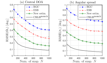
Figure 1: RMSE of the three estimators versus $N$ for SNR $=5$ dB.

Clearly, our estimator is statistically more efficient and outperforms ESB and RGC both in terms of central DOAs and angular spreads estimation accuracy. Moreover, the performance improvements of the proposed method over ESB and RGC hold almost the same irrespectively of $N$. Therefore, we will hereafter fix $N=1000$.
Figs. 2(a) and 2(b) depict the empirical RMSEs of all tested methods versus the SNR. The analytical RMSE of the new estimator established in Section V is also plotted there. These figures show a very good agreement between the empirical and analytical RMSEs of the proposed estimator, thereby corroborating our analytical performance analysis of Section V. It also suggests that the proposed estimator outperforms ESB and RGC, both in terms of central DOAs and angular spreads estimation capabilities, especially under the adverse conditions of low SNR levels.

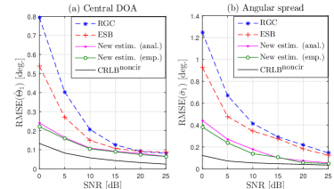
Figure 2: RMSE of the three estimators versus SNR for $N=1000$, sources with the same angular distribution.

In Fig. 3, we consider two uncorrelated ID noncircular sources with different angular distributions. More specifically, the first source is uniformly distributed (UID) with central DOA, $\bar{\Theta}_{1}=10{\textrm{\textdegree}}$, and angular spread $\bar{\sigma}_{1}=1.5{\textrm{\textdegree}}$ while the second is GID distributed with central DOA, $\bar{\Theta}_{2}=30{\textrm{\textdegree}}$, and angular spread $\bar{\sigma}_{2}=3{\textrm{\textdegree}}$.

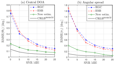
Figure 3: RMSE of the three estimators versus SNR for $N=1000$, sources with different angular distributions.

To apply ESB in this setup, however, we assume that both sources are GID. In fact, in contrast to the proposed method and RGC, ESB was specifically derived in the case where all the sources have the same angular distribution. By comparing Figs. 2 and 3 (i.e., sources truly having the same distribution), we observe that ESB suffers from severe performance degradation. It even becomes less accurate than RGC at low SNR levels, that is in stark contrast to what was earlier reported in Fig. 2. The proposed estimator, however, keeps its superiority in terms of estimation accuracy thereby making it more attractive in practice where the sources are more likely to have different angular distributions.
Next, we examine the impact of the sources’ separation on the performance of the three estimators. To that end, we reconsider the case of noncircular ID sources with the same angular distribution (GID). The first source is kept fixed at $\bar{\Theta}_{1}=10{\textrm{\textdegree}}$ with angular spread, $\bar{\sigma}_{1}=1.5{\textrm{\textdegree}}$, while the second (with $\bar{\sigma}_{2}=3^{\circ}$) is shifted from $18{\textrm{\textdegree}}$ to $30{\textrm{\textdegree}}$ with $2^{\circ}$. The results are plotted in Fig. 4 at $5$ dB SNR and suggest that all estimators expectedly improve their accuracy as the DOA separation increases. Yet, the proposed approach significantly outperforms ESB and RGC for small DOA separations, a more challenging scenario in practice.

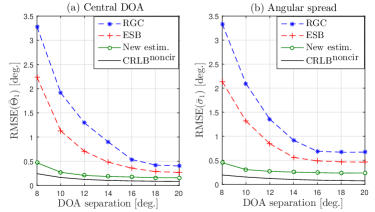
Figure 4: RMSE of the three estimators versus DOA separation for $N=1000$ and SNR $=5$ dB, sources with the same angular distributions.

Finally, we consider in Fig. 5 an even more challenging scenario where two uncorrelated GID noncircular sources with the same noncircularity rate ($\gamma_{1}=\gamma_{2}=1$) and noncircularity phases $\varphi_{1}=\frac{\pi}{3}$ and $\varphi_{2}=\frac{\pi}{4}$ are located at central DOAs $\bar{\Theta}_{1}=10{\textrm{\textdegree}}$ and $\bar{\Theta}_{2}=15{\textrm{\textdegree}}$ with respective angular spreads $\bar{\sigma}_{1}=2{\textrm{\textdegree}}$ and $\bar{\sigma}_{2}=4{\textrm{\textdegree}}$. The number of snapshots is fixed to $N=100$. Figs. 5(a) and 5(b) show that the performance of the three methods is satisfactory, especially at high SNR values. However, our new estimator still outperforms the two other methods both in terms of central DOAs and angular spreads estimation performance.

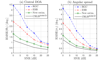
Figure 5: RMSE of the three estimators versus $SNR$ for $N=100$, sources with the same angular distributions.

VII-B Assessment of the new CRLBs:

In this subsection, we illustrate the newly derived CRLBs (i.e., $\textrm{CRLB}^{\textrm{noncir}}$) in different scenarios. We first consider two equipowered ID sources with identical noncircularity rate, $\gamma=1$, and noncircularity phases $\varphi_{1}=\pi/3$ and $\varphi_{2}=\pi/4$. The sources are located at central DOAs $\bar{\Theta}_{1}=10{\textrm{\textdegree}}$ and $\bar{\Theta}_{2}=30{\textrm{\textdegree}}$ with respective angular spreads $\bar{\sigma}_{1}=3{\textrm{\textdegree}}$ and $\bar{\sigma}_{2}=5{\textrm{\textdegree}}$. Figs. 6(a) and 6(b) show both $\log(\textrm{CRLB}^{\textrm{noncir}})$ and $\log(\textrm{CRLB}^{\textrm{cir}})$ of $\bar{\Theta}_{1}$ and $\bar{\sigma}_{1}$, respectively, when the sources have: $i$) the same Gaussian angular distribution, and $ii$) different angular distributions (the first source is UID and the second source is GID).

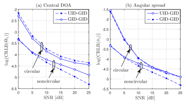
Figure 6: $\textrm{CRLB}^{\textrm{noncir}}$ and $\textrm{CRLB}^{\textrm{cir}}$ as function the SNR.

We see from Fig. 6 that the CRLBs for noncircular ID sources are lower than their counterparts derived assuming ID circular sources, especially at low SNR values. This illustrates the performance gain that is achieved by exploiting the non-circularity feature of the sources in the estimation process. Moreover, $\textrm{CRLB}^{\textrm{cir}}$ converges faster to $\textrm{CRLB}^{\textrm{noncir}}$, at high SNR, when the sources have the same angular distribution (GID-GID in our case). Therefore, at high SNRs, the noncircularity of the signals is more informative about the angular parameters when the sources have different distributions. Next, we examine the impact of the angular spread on the estimation of the angular parameters, by fixing $\bar{\sigma}_{2}$ and varying $\bar{\sigma}_{1}$. Fig. 7 depicts $\log(\textrm{CRLB}^{\textrm{noncir}})$ and $\log(\textrm{CRLB}^{\textrm{cir}})$ as a function of the SNR for three different values of $\bar{\sigma}_{1}$. Moreover, we consider in Fig. 7(a) the case of point (or non-distributed) sources which corresponds to $\bar{\sigma}_{1}=\bar{\sigma}_{2}=0{\textrm{\textdegree}}$.

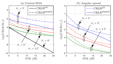
Figure 7: $\textrm{CRLB}^{\textrm{noncir}}$ and $\textrm{CRLB}^{\textrm{cir}}$ versus the SNR for different values of $\bar{\sigma}_{1}$.

As intuitively expected, $\textrm{CRLB}^{\textrm{noncir}}$ and $\textrm{CRLB}^{\textrm{cir}}$ increase with the angular spread and so does the difference between them. This reveals that as the angular spread increases, there is more room for the noncircularity of the signals to improve the estimation performance. In fact, the signals become more dispersed and thus the unconjugated covariance matrix becomes more informative about the angular parameters. In Figs. 8 and 9, we study the effect of the signals’ noncircularity parameters on CRLB${}^{\textrm{noncir}}$ under different sources’ separations, $\Delta\Theta$, in terms of central DOAs. The first source is UID and fixed at $\bar{\Theta}_{1}=10{\textrm{\textdegree}}$ whereas the second source is GID and its central DOA, $\bar{\Theta}_{2}$, is varied from $18{\textrm{\textdegree}}$ to $30{\textrm{\textdegree}}$.

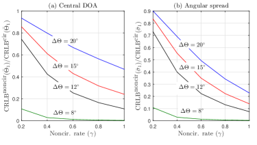
Figure 8: Ratio of CRLBs as a function of the noncircularity rate $\gamma$ for different values of DOA separation ($\Delta\Theta$), $\bar{\sigma}_{1}=3^{\circ}$, $\bar{\sigma}_{2}=5^{\circ}$, $\varphi_{1}=\pi/3$, $\varphi_{2}=\pi/4$, $N=1000$, and SNR $=5$ dB.

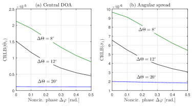
Figure 9: $\textrm{CRLB}^{\textrm{noncir}}(\bar{\Theta}_{1})$ and $\textrm{CRLB}^{\textrm{noncir}}(\sigma_{1})$ as a function of the noncircularity phase $\Delta\varphi$ for different values of DOA separation ($\Delta\Theta$) for $\bar{\sigma}_{1}=3^{\circ}$, $\bar{\sigma}_{2}=5^{\circ}$, $\gamma=1$, $N=1000$, and SNR $=5$ dB.

We observe from Figs. 8-(a) and 8-(b) that $\textrm{CRLB}^{\textrm{noncir}}$ of the two angular parameters decrease as the noncircularity steps rate increases. Moreover, the gap between $\textrm{CRLB}^{\textrm{noncir}}$ and $\textrm{CRLB}^{\textrm{cir}}$ increases as the DOA separation $\Delta\Theta$ decreases. In fact, the ratio between the two CRLBs tends to zero at low DOA separations (for $\Delta\Theta=8^{\circ}$). More specifically, at low DOA separations, $\textrm{CRLB}^{\textrm{noncir}}$ becomes very small compared to $\textrm{CRLB}^{\textrm{cir}}$, meaning that huge performance gains can be achieved in this challenging scenario by exploiting the additional information carried by the unconjugated covariance matrix. Fig. 9 also reveals that $\textrm{CRLB}^{\textrm{noncir}}$ is more sensitive to the noncircularity phase separation at small DOA separations.

VIII Conclusion

In this paper, we developed a new method for the estimation of the angular parameters in the presence of noncircular ID sources. The new estimator decouples the estimation of the central DOAs from that of the angular spreads by means of two consecutive 1-D searches, thereby resulting in tremendous computational savings as compared to the brute-force 2D grid search solution. It is also oblivious to the sources’ angular distribution or any mismatch thereof. This estimator is particulary interessant for symmetric sources’ distributions with small angular spreads.
The proposed estimator outperforms most recent state-of-the-art techniques, especially for small DOA separations and/or low SNR levels. Its performance was also assessed analytically and the obtained results were corroborated by Monte-Carlo simulations. In order to benchmark the new estimator, we also derived for the first time an explicit expression for the stochastic CRLBs of the underlying estimation problem. The analysis of the new CRLB unambiguously shows that the noncircularity of the signals brings valuable additional information about the angular parameters especially when the sources have different angular distributions and/or when the angular spreads increase. Besides, the noncircular CRLBs decrease as the noncircularity rate increases. And, they are much smaller than the circular CRLBs at small DOA separations. In which case they also become more sensitive to the noncircularity phase separation.

Appendix A—Proof of (III)

From (45), the $(p,l)$th element of $\mathbf{R}_{ss}(\bar{\bm{\psi}}_{k})$ has the following expression:

$$\big{[}\mathbf{R}_{ss}\big{]}_{pl}(\bar{\bm{\psi}}_{k}) = \int\rho_{k}(\theta,\bar{\bm{\psi}}_{k})a_{p}(\theta)a_{l}^{*}(\theta)d\theta,$$ (124)

where $a_{p}(\theta)=e^{j2\pi f_{p-1}(\theta)}$. Otherwise, we denote by $\widetilde{\theta}$ the deviation of the direction $\theta$ from the central DOA $\bar{\Theta}_{k}$ as follows:

$$\widetilde{\theta} = \theta-\bar{\Theta}_{k}.$$ (125)

For small angular spreads, $\widetilde{\theta}$ tends to zero. We can therefore use the following approximation:

$$f_{p-1}(\theta) \simeq f_{p-1}(\bar{\Theta}_{k})+\widetilde{\theta}f^{\prime}_{p-1}(\bar{\Theta}_{k}),$$ (126)

where $f^{\prime}_{p-1}(\theta)$ stands for the first derivative of $f_{p-1}(\theta)$ with respect to $\theta$. Hence, we obtain the following expression for $\big{[}\mathbf{R}_{ss}\big{]}_{pl}(\bar{\bm{\psi}}_{k})$:

$$\!\!\!\!\!\!\!\!\!\!\!\!\big{[}\mathbf{R}_{ss}\big{]}_{pl}(\bar{\bm{\psi}}_{k}) \!\!\!\!\!\simeq\!\!\!\!\! e^{j2\pi(f_{p-1}\left(\bar{\Theta}_{k})-f_{l-1}(\bar{\Theta}_{k})\right)}$$ (127)

$$\!\!\!\!\!\times\!\!\!\!\! \!\!\int\!\!\!\rho_{k}(\bar{\Theta}_{k}+\widetilde{\theta},\bar{\bm{\psi}}_{k})e^{j2\pi\left(f^{\prime}_{p-1}(\bar{\Theta}_{k})-f^{\prime}_{l-1}(\bar{\Theta}_{k})\right)\widetilde{\theta}}d\widetilde{\theta}.$$

$\big{[}\mathbf{R}_{ss}\big{]}_{pl}(\bar{\bm{\psi}}_{k})$ can be written equivalently as follows:

$$\big{[}\mathbf{R}_{ss}\big{]}_{pl}(\bar{\bm{\psi}}_{k}) \!\!\!\simeq\!\!\! \Big{(}\mathbf{a}(\bar{\Theta}_{k})\!~{}\mathbf{a}(\bar{\Theta}_{k})^{H}\Big{)}_{pl}\times\big{[}\mathbf{T}\big{]}_{pl}(\bar{\bm{\psi}}_{k}),$$ (128)

where $\big{[}\mathbf{T}\big{]}_{pl}(\bar{\bm{\psi}}_{k})$ is given by:

$$\!\!\!\!\!\!\!\![\mathbf{T}]_{pl}(\bar{\bm{\psi}}_{k}) \!\!\!\!\!=\!\!\!\!\!\!\! \int\!\!\rho_{k}(\bar{\Theta}_{k}+\widetilde{\theta},\bar{\bm{\psi}}_{k})e^{j2\pi\left(f^{\prime}_{p-1}(\bar{\Theta}_{k})-f^{\prime}_{l-1}(\bar{\Theta}_{k})\right)\widetilde{\theta}}d\widetilde{\theta}.$$ (129)

From (129), the complex conjugate of $[\mathbf{T}]_{pl}(\bar{\bm{\psi}}_{k})$ is given by:

$$[\mathbf{T}]^{*}_{pl}(\bar{\bm{\psi}}_{k}) \!\!\!=\!\!\! \int\rho_{k}(\bar{\Theta}_{k}+\widetilde{\theta},\bar{\bm{\psi}}_{k})e^{-j2\pi\left(f^{\prime}_{p-1}(\bar{\Theta}_{k})-f^{\prime}_{l-1}(\bar{\Theta}_{k})\right)\widetilde{\theta}}d\widetilde{\theta},$$ (130)

$$\!\!\!=\!\!\! \int\rho_{k}(\bar{\Theta}_{k}+\widetilde{\theta},\bar{\bm{\psi}}_{k})e^{j2\pi\left(f^{\prime}_{p-1}(\bar{\Theta}_{k})-f^{\prime}_{l-1}(\bar{\Theta}_{k})\right)\widetilde{\theta}}d\widetilde{\theta},$$

$$\!\!\!=\!\!\! [\mathbf{T}]_{lp}(\bar{\bm{\psi}}_{k}).$$

Moreover, by assuming that the angular distribution is symmetric with respect to the central DOA $\bar{\Theta}_{k}$, we have the following relation:

$$\rho_{k}(\theta,\bar{\bm{\psi}}_{k}) = \rho_{k}(\bar{\Theta}_{k}+\widetilde{\theta},\bar{\bm{\psi}}_{k})=\rho_{k}(\bar{\Theta}_{k}-\widetilde{\theta},\bar{\bm{\psi}}_{k}).$$ (131)

From (131), it follows that:

$$[\mathbf{T}]^{*}_{pl}(\bar{\bm{\psi}}_{k}) \!\!\!\!\!=\!\!\!\!\!\!\! \int_{-\infty}^{+\infty}\!\!\!\!\rho_{k}(\bar{\Theta}_{k}+\widetilde{\theta},\bar{\bm{\psi}}_{k})e^{j2\pi\left(f^{\prime}_{p-1}(\bar{\Theta}_{k})-f^{\prime}_{l-1}(\bar{\Theta}_{k})\right)(-\widetilde{\theta})}d\widetilde{\theta},$$ (132)

$$\!\!\!\!\!=\!\!\!\!\!\!\! \int_{+\infty}^{-\infty}\!\!\!\!\!\!\!\!\!\!\rho_{k}(\bar{\Theta}_{k}-\widetilde{\theta_{1}},\bar{\bm{\psi}}_{k})e^{j2\pi\left(f^{\prime}_{p-1}(\bar{\Theta}_{k})-f^{\prime}_{l-1}(\bar{\Theta}_{k})\right)\widetilde{\theta_{1}}}(-d\widetilde{\theta_{1}}),$$

$$\!\!\!\!\!=\!\!\!\!\!\!\! \int_{-\infty}^{+\infty}\!\!\!\!\rho_{k}(\bar{\Theta}_{k}+\widetilde{\theta_{1}},\bar{\bm{\psi}}_{k})e^{j2\pi\left(f^{\prime}_{p-1}(\bar{\Theta}_{k})-f^{\prime}_{l-1}(\bar{\Theta}_{k})\right)\widetilde{\theta_{1}}}d\widetilde{\theta_{1}},$$

$$\!\!\!\!\!=\!\!\!\!\! [\mathbf{T}]_{pl}(\bar{\bm{\psi}}_{k}).$$

From (130) and (132), we have that:

$$[\mathbf{T}]^{*}_{pl}(\bar{\bm{\psi}}_{k}) = [\mathbf{T}]_{pl}(\bar{\bm{\psi}}_{k})=[\mathbf{T}]_{lp}(\bar{\bm{\psi}}_{k}).$$ (133)

This proves that $\mathbf{T}(\bar{\bm{\psi}}_{k})$ is a real-valued $(L\times L)$ symmetric matrix. Otherwise, $\exp\{j2\pi\left(f^{\prime}_{p-1}(\bar{\Theta}_{k})-f^{\prime}_{l-1}(\bar{\Theta}_{k})\right)\widetilde{\theta}\}$ can be written as:

$$e^{j2\pi\left(f^{\prime}_{p-1}(\bar{\Theta}_{k})-f^{\prime}_{l-1}(\bar{\Theta}_{k})\right)\widetilde{\theta}} \!\!\!\!=\!\!\!\! \cos\!\left(\!2\pi\big{(}f^{\prime}_{p-1}(\bar{\Theta}_{k})-f^{\prime}_{l-1}(\bar{\Theta}_{k})\big{)}\widetilde{\theta}\right)$$

$$\!\!\!\!+\!\!\!\! j\sin\!\left(\!2\pi\big{(}f^{\prime}_{p-1}(\bar{\Theta}_{k})-f^{\prime}_{l-1}(\bar{\Theta}_{k})\big{)}\widetilde{\theta}\right).$$

Therefore, $[\mathbf{T}]_{pl}(\bar{\bm{\psi}}_{k})$ can be expressed as follows:

$$[\mathbf{T}]_{pl}(\bar{\bm{\psi}}_{k}) \!\!\!\!\!\!=\!\!\!\!\!\!\!\! \int\!\!\rho_{k}(\bar{\Theta}_{k}+\widetilde{\theta},\bar{\bm{\psi}}_{k})\cos\!\left(\!2\pi\big{(}f^{\prime}_{p-1}(\bar{\Theta}_{k})-f^{\prime}_{l-1}(\bar{\Theta}_{k})\big{)}\widetilde{\theta}\right)\!d\widetilde{\theta}$$

$$\!\!\!\!\!\!+\!\!\!\!\!\! j\!\!\int\!\!\rho_{k}(\bar{\Theta}_{k}+\widetilde{\theta},\bar{\bm{\psi}}_{k})\sin\!\left(\!2\pi\big{(}f^{\prime}_{p-1}(\bar{\Theta}_{k})-f^{\prime}_{l-1}(\bar{\Theta}_{k})\big{)}\widetilde{\theta}\right)\!d\widetilde{\theta}.$$

Since $\mathbf{T}(\bar{\bm{\psi}}_{k})$ is a real-valued matrix, then we can deduce that:

$$\!\!\!\!\!\!\!\!\!\!\int\!\!\rho_{k}(\bar{\Theta}_{k}+\widetilde{\theta},\bar{\bm{\psi}}_{k})\sin\!\left(\!2\pi\big{(}f^{\prime}_{p-1}(\bar{\Theta}_{k})-f^{\prime}_{l-1}(\bar{\Theta}_{k})\big{)}\widetilde{\theta}\right)\!d\widetilde{\theta} \!\!\!\!\!\!=\!\!\!\!\!\! 0.$$ (134)

Consequently, $[\mathbf{T}]_{pl}(\bar{\bm{\psi}}_{k})$ can be reduced to:

$$[\mathbf{T}]_{pl}(\bar{\bm{\psi}}_{k}) \!\!\!\!\!\!=\!\!\!\!\!\!\!\! \int\rho_{k}(\bar{\Theta}_{k}+\widetilde{\theta},\bar{\bm{\psi}}_{k})\!\cos\!\left(2\pi\big{(}f^{\prime}_{p-1}(\bar{\Theta}_{k})\!-\!f^{\prime}_{l-1}(\bar{\Theta}_{k})\big{)}\widetilde{\theta}\right)\!d\widetilde{\theta},$$

$$\!\!\!\!\!\!=\!\!\!\!\!\!\!\! \int\!\!\rho_{k}(\theta,\bar{\bm{\psi}}_{k})\!\cos\!\left(2\pi(f^{\prime}_{p-1}(\bar{\Theta}_{k})\!-\!f^{\prime}_{l-1}(\bar{\Theta}_{k}))(\theta\!-\!\bar{\Theta}_{k})\right)\!d\theta,$$

thereby leading to the result given in (III). Moreover, since, we have:

$$\cos\!\left(2\pi(f^{\prime}_{p-1}(\bar{\Theta}_{k})\!-\!f^{\prime}_{l-1}(\bar{\Theta}_{k}))(\theta\!-\!\bar{\Theta}_{k})\right) \leq 1,$$ (135)

then we can conclude that $\forall p,l$, we have:

$$[\mathbf{T}]_{pl}(\bar{\bm{\psi}}_{k}) \leq \int\rho_{k}(\theta,\bar{\bm{\psi}}_{k})d\theta=1.$$ (136)

Appendix B—Proof of (154)

Substituting (51) in (39) and using the identity $\textrm{tr}\{\mathbf{A}\mathbf{B}\mathbf{C}\}=\textrm{tr}\{\mathbf{C}\mathbf{A}\mathbf{B}\}$ for any square matrices, $\mathbf{A},\mathbf{B}$ and $\mathbf{C}$, along with the fact that $\widetilde{\bm{\Phi}}(\bar{\Theta},\varphi)^{H}\widetilde{\bm{\Phi}}(\bar{\Theta},\varphi)=\mathbf{I}_{2L}$, we obtain:

$$\!\!\!\!\!\!\!\!\!\!f\big{(}\bm{\psi},\varphi\!~{}\big{|}\!~{}\widehat{\mathbf{R}}_{\widetilde{\mathbf{x}}\widetilde{\mathbf{x}}}^{-2}\big{)} = \textrm{tr}\left\{\widetilde{\bm{\Phi}}(\bar{\Theta},\varphi)\widetilde{\mathbf{T}}^{2}(\bm{\psi})\widetilde{\bm{\Phi}}(\bar{\Theta},\varphi)^{H}\widehat{\mathbf{R}}_{\widetilde{\mathbf{x}}\widetilde{\mathbf{x}}}^{-2}\right\}.$$ (137)

On the other hand, by recalling the expression of the extended array response vector, $\widetilde{\mathbf{a}}(\bar{\Theta},\varphi)$, in (27), it follows that $\widetilde{\bm{\Phi}}(\bar{\Theta},\varphi)=\textrm{diag}\{\widetilde{\mathbf{a}}(\bar{\Theta},\varphi)\}$ is given by:

$$\!\!\!\!\!\!\!\!\!\widetilde{\bm{\Phi}}(\bar{\Theta},\varphi) \!\!=\!\! \left(\!\!\begin{array}[]{ccc}\textrm{diag}\big{\{}\mathbf{a}(\bar{\Theta})\big{\}}&{}{}\hfil&\bm{0}_{L\times L}\\ \\ \bm{0}_{L\times L}&{}{}\hfil&e^{-j\varphi}\textrm{diag}\big{\{}\mathbf{a}(\bar{\Theta})\big{\}}^{H}\end{array}\!\!\right)\!\!.$$ (141)

Furthermore, by recalling the expression of $\widetilde{\mathbf{T}}(\bm{\psi})$ in (55), it is easy to show that:

$$\widetilde{\mathbf{T}}(\bm{\psi})^{2} = \left(\!\!\begin{array}[]{cc}\mathbf{A}(\bm{\psi})~{}~{}~{}~{}~{}~{}\mathbf{B}(\bm{\psi})\\ \mathbf{B}(\bm{\psi})~{}~{}~{}~{}~{}\mathbf{A}(\bm{\psi})\end{array}\!\!\right),$$ (144)

where

$$\mathbf{A}(\bm{\psi}) = \mathbf{T}(\bm{\psi})^{2}~{}+~{}{\mathbf{T}^{\prime}}(\bm{\psi})^{2},$$

$$\mathbf{B}(\bm{\psi}) = \mathbf{T}(\bm{\psi}){\mathbf{T}^{\prime}}(\bm{\psi})~{}+~{}{\mathbf{T}^{\prime}}(\bm{\psi})\mathbf{T}(\bm{\psi}).$$

Similar to (30), the estimated extended covariance matrix, $\widehat{\mathbf{R}}_{\widetilde{\mathbf{x}}\widetilde{\mathbf{x}}}$, is eigendecomposed as follows:

$$\!\!\!\!\!\!\!\!\widehat{\mathbf{R}}_{\widetilde{\mathbf{x}}\widetilde{\mathbf{x}}} = \widehat{\widetilde{\mathbf{U}}}_{s}\widehat{\bm{\Sigma}}_{s}\widehat{\widetilde{\mathbf{U}}}_{s}^{H}~{}+~{}\widehat{\widetilde{\mathbf{U}}}_{w}\widehat{\bm{\Sigma}}_{w}\widehat{\widetilde{\mathbf{U}}}_{w}^{H},$$ (145)

from which it can be shown that:

$$\widehat{\mathbf{R}}_{\widetilde{\mathbf{x}}\widetilde{\mathbf{x}}}^{-2} = \widehat{\widetilde{\mathbf{U}}}_{s}\widehat{\bm{\Sigma}}_{s}^{-2}\widehat{\widetilde{\mathbf{U}}}_{s}^{H}~{}+~{}\widehat{\widetilde{\mathbf{U}}}_{w}\widehat{\bm{\Sigma}}_{w}^{-2}\widehat{\widetilde{\mathbf{U}}}_{w}^{H}.$$ (146)

Moreover, as shown in [References], $\widehat{\widetilde{\mathbf{U}}}_{s}$ and $\widehat{\widetilde{\mathbf{U}}}_{w}$ can be partitioned as follows:

$$\!\!\!\!\!\!\!\!{\widehat{\widetilde{\mathbf{U}}}_{s}} = [{\widehat{\mathbf{U}}_{s}^{T}},{\widehat{\mathbf{U}}_{s}^{{}^{\prime}T}}]^{T}~{}~{}~{}~{}~{}~{}~{}\textrm{with}~{}~{}~{}~{}~{}~{}~{}\widehat{\mathbf{U}}_{s}^{{}^{\prime}}~{}=~{}\widehat{\mathbf{U}}_{s}^{*}\mathbf{D}_{s},$$ (147)

$$\!\!\!\!\!\!\!\!{\widehat{\widetilde{\mathbf{U}}}_{w}} = [{\widehat{\mathbf{U}}_{w}^{T}},{\widehat{\mathbf{U}}_{w}^{{}^{\prime}T}}]^{T}~{}~{}~{}~{}~{}~{}~{}\textrm{with}~{}~{}~{}~{}~{}~{}~{}\widehat{\mathbf{U}}_{w}^{{}^{\prime}}~{}=~{}\widehat{\mathbf{U}}_{w}^{*}\mathbf{D}_{w},$$ (148)

where $\mathbf{D}_{s}$ and $\mathbf{D}_{w}$ are some diagonal matrices whose complex diagonal entries are of unit modulus. Injecting (147) and (148) back into (146), we show after some algebraic manipulations that $\widehat{\mathbf{R}}_{\widetilde{\mathbf{x}}\widetilde{\mathbf{x}}}^{-2}$ has the following block diagonal structure:

$$\widehat{\mathbf{R}}_{\widetilde{\mathbf{x}}\widetilde{\mathbf{x}}}^{-2} = \left(\!\!\begin{array}[]{cc}\widehat{\mathbf{R}}_{1}~{}~{}~{}~{}~{}\widehat{\mathbf{R}}_{2}\\ \widehat{\mathbf{R}}_{2}^{*}~{}~{}~{}~{}~{}\widehat{\mathbf{R}}_{1}^{*}\end{array}\!\!\right),$$ (151)

where

$$\widehat{\mathbf{R}}_{1} = \widehat{\mathbf{U}}_{s}\widehat{\bm{\Sigma}}^{-2}_{s}\widehat{\mathbf{U}}_{s}^{H}~{}~{}+~{}~{}\widehat{\mathbf{U}}_{w}\widehat{\bm{\Sigma}}_{w}\widehat{\mathbf{U}}_{w}^{H},$$ (152)

$$\widehat{\mathbf{R}}_{2} = \widehat{\mathbf{U}}_{s}\widehat{\bm{\Sigma}}^{-2}_{s}\mathbf{D}_{s}^{*}\widehat{\mathbf{U}}_{s}^{T}~{}~{}+~{}~{}\widehat{\mathbf{U}}_{n}\widehat{\bm{\Sigma}}_{w}\mathbf{D}_{w}^{*}\widehat{\mathbf{U}}_{w}^{T}.$$ (153)

Substituting (141), (144), and (151) back into (137), and resorting to some algebraic manipulations yields the following result:

$$\!\!\!\!\!\!\!\!\!\!f\big{(}\bm{\psi},\varphi\big{|}\!~{}\widehat{\mathbf{R}}_{\widetilde{\mathbf{x}}\widetilde{\mathbf{x}}}^{-2}\big{)} = 2\Re\Big{\{}~{}\!z_{1}(\bm{\psi})~{}\!+~{}\!e^{j\varphi}z_{2}(\bm{\psi})~{}\!\Big{\}}~{},$$ (154)

in which the complex numbers $z_{1}(\bm{\psi})$ and $z_{2}(\bm{\psi})$ are explicitly given by:

$$\!\!\!\!\!\!\!\!z_{1}(\bm{\psi}) = \textrm{tr}\Big{\{}\textrm{diag}\{\mathbf{a}(\Theta)\}\mathbf{A}(\bm{\psi})\textrm{diag}\left\{\mathbf{a}(\Theta)^{H}\right\}\widehat{\mathbf{R}}_{1}\Big{\}},$$ (155)

$$\!\!\!\!\!\!\!\!z_{2}(\bm{\psi}) = \textrm{tr}\Big{\{}\textrm{diag}\{\mathbf{a}(\Theta)\}\mathbf{B}(\bm{\psi})\textrm{diag}\left\{\mathbf{a}(\Theta)^{T}\right\}\widehat{\mathbf{R}}_{2}^{*}\Big{\}}.$$ (156)

In order to reduce the dimensionality of the optimization problem at hand, we begin by minimizing the underlying cost function with respect to the unknown noncircularity phase $\varphi$. To that end, we use $z_{2}(\bm{\psi})=|z_{2}(\bm{\psi})|{\exp\{j\angle z_{2}(\bm{\psi})}\}$ and rewrite (154) as follows:

$$\!\!\!\!\!\!\!f\big{(}\bm{\psi},\varphi\!~{}\big{|}\!~{}\widehat{\mathbf{R}}_{\widetilde{\mathbf{x}}\widetilde{\mathbf{x}}}^{-2}\big{)}$$ (158)

$$\!\!\!\!\!\!\!\!\!\!\!\!\!\!\!\!\!\!\!\!\!\!\!\!\!\!\!\!\!=~{}2\Re\big{\{}z_{1}(\bm{\psi})\big{\}}~{}\!+~{}\!2|z_{2}(\bm{\psi})|\Re\big{\{}{e^{j\angle z_{2}(\bm{\psi})}}{e^{j\varphi}}~{}\!\Big{\}}~{},$$

$$\!\!\!\!\!\!\!\!\!\!\!\!\!\!\!\!\!\!\!\!\!\!\!\!\!\!\!\!\!=~{}2\Re\big{\{}z_{1}(\bm{\psi})\big{\}}~{}\!+~{}\!2|z_{2}(\bm{\psi})|\cos\big{(}\varphi+\angle z_{2}(\bm{\psi})\big{)}.$$

From (158), it is clear (for a fixed $\bm{\psi}$) that the function $f(.)$ attains its minimum (with respect to $\varphi$) at the point:

$$\widehat{\varphi}(\bm{\psi}) = \pi~{}-~{}\angle~{}\!z_{2}(\bm{\psi}).$$ (159)

Substituting (159) back into (158) and recalling (155) and (156), we obtain the following cost function that depends on $\bm{\psi}$ only:

$$\!\!\!\!\!\!\!\!\!\!\!\!f_{c}\big{(}\bm{\psi}\!~{}\big{|}\!~{}\widehat{\mathbf{R}}_{\widetilde{\mathbf{x}}\widetilde{\mathbf{x}}}^{-2}\big{)}$$ (160)

$$\!\!\!\!\!\!\!\!\!\!\!\!\!\!\!\!\!\!\!\!\!\!\!\!=~{}\!\Re\bigg{\{}\textrm{tr}\Big{\{}\textrm{diag}\big{\{}\mathbf{a}(\Theta)\big{\}}\mathbf{A}(\bm{\psi})\textrm{diag}\big{\{}\mathbf{a}(\Theta)^{H}\big{\}}\widehat{\mathbf{R}}_{1}\Big{\}}\bigg{\}}$$

$$\!\!\!\!\!\!-\bigg{|}~{}\!\textrm{tr}\Big{\{}\textrm{diag}\big{\{}\mathbf{a}(\Theta)\big{\}}\mathbf{B}(\bm{\psi})\textrm{diag}\big{\{}\mathbf{a}(\Theta)\big{\}}^{T}\widehat{\mathbf{R}}_{2}^{*}\Big{\}}\bigg{|},$$

which is equivalent to the result given in (60).

Appendix C—Proof of (66) and (77)

$\mathbf{T}(\bm{\psi})$ is a symmetric Toeplitz matrix constructed from its first column vector $\mathbf{t}_{1}$ as follows:

$$\mathbf{T}(\bm{\psi}) = \textrm{Toeplitz}\big{(}\mathbf{t}_{1}\big{)},$$ (161)

where the $l$th element of the vector $\mathbf{t}_{1}$ is given from (62) by:

$$\!\!\!\!\mathbf{t}_{1}(l) \!\!\!\!\!\!=\!\!\!\!\!\! [\mathbf{T}]_{l1}(\bar{\bm{\psi}}_{k}),$$ (162)

$$\!\!\!\!\!\!=\!\!\!\!\!\! \int\!\rho_{k}(\theta,\bar{\bm{\psi}}_{k})\cos\left(2\pi(l-1)g(\bar{\Theta}_{k})\!(\theta\!-\!\bar{\Theta}_{k})\right)\!d\theta.$$

For small angular spreads, we use a second-order Taylor-series development of $\cos\left(2\pi(l-1)g(\bar{\Theta}_{k})\!(\theta\!-\!\bar{\Theta}_{k})\right)$ to obtain the following equality:

$$\cos\!\left(2\pi(l-1)g(\bar{\Theta}_{k}))\!(\theta\!-\!\bar{\Theta}_{k})\right) \!\!\!\!\!\simeq\!\!\!\!\! 1-2\pi^{2}(l-1)^{2}g^{2}(\bar{\Theta}_{k}))\!(\theta\!-\!\bar{\Theta}_{k})^{2}.$$

Then, $\mathbf{t}_{1}(l)$ can be approximated as follows:

$$\mathbf{t}_{1}(l) \!\!\!\!\!\simeq\!\!\!\!\!\!\! \int\!\!\rho_{k}(\theta,\bar{\bm{\psi}}_{k})d\theta-2\pi^{2}(l-1)^{2}g^{2}(\bar{\Theta}_{k})\!\!\int\!(\theta\!-\!\bar{\Theta}_{k})^{2}\rho_{k}(\theta,\bar{\bm{\psi}}_{k})d\theta,$$ (163)

$$\!\!\!\!\!=\!\!\!\!\! 1-2\pi^{2}(l-1)^{2}g^{2}(\bar{\Theta}_{k})\bar{\sigma}_{k}^{2}.$$

From (163), we clearly see that the elements, $\{\mathbf{t}_{1}(l)\}_{l=1}^{L}$, of the vector, $\mathbf{t}_{1}$, satisfy the following property:

$$1~{}=~{}\mathbf{t}_{1}(1)~{}\geq~{}\mathbf{t}_{1}(2)~{}\geq\ldots\geq~{}\mathbf{t}_{1}(L).$$ (164)

Moreover, if $\sigma<1/\big{(}\sqrt{2}\pi(l-1)g(\bar{\Theta}_{k})\big{)}~{}\forall~{}\!l=1,\ldots,L$ or equivalently $\sigma<1/\big{(}\sqrt{2}\pi(L-1)g(\bar{\Theta}_{k})\big{)}$, then $\mathbf{t}_{1}(L)\geq 0$.
In the same way, ${\mathbf{T}^{\prime}}(\bm{\psi})$ is a Hankel matrix defined from its first and last column vectors $\mathbf{t}^{\prime}_{1}$ and $\mathbf{t}^{\prime}_{L}$ as follows:

$$\mathbf{T}^{\prime}(\bm{\psi}) = \textrm{Hankel}\big{(}\mathbf{t}^{\prime}_{1},\mathbf{t}^{\prime}_{L}\big{)},$$ (165)

where the $l$th elements of the vectors $\mathbf{t}^{\prime}_{1}$ and $\mathbf{t}^{\prime}_{L}$ are given, respectively, by:

$$\!\!\!\!\!\!\!\!\mathbf{t}^{\prime}_{1}(l) \!\!\!\!\!=\!\!\!\!\! [\mathbf{T}^{\prime}]_{l1}(\bar{\bm{\psi}}_{k}),$$ (166)

$$\!\!\!\!\!=\!\!\!\!\! \int\!\!\rho_{k}(\theta,\bar{\bm{\psi}}_{k})\cos\!\left(2\pi(l+1-2)g(\bar{\Theta}_{k})\!(\theta\!-\!\bar{\Theta}_{k})\right)\!d\theta,$$

$$\!\!\!\!\!=\!\!\!\!\! \int\!\!\rho_{k}(\theta,\bar{\bm{\psi}}_{k})\cos\!\left(2\pi(l-1)g(\bar{\Theta}_{k})\!(\theta\!-\!\bar{\Theta}_{k})\right)\!d\theta,$$

$$\!\!\!\!\!\!\!\!\mathbf{t}^{\prime}_{L}(l) \!\!\!\!\!=\!\!\!\!\! [\mathbf{T}^{\prime}]_{lL}(\bar{\bm{\psi}}_{k}),$$ (167)

$$\!\!\!\!\!=\!\!\!\!\! \int\!\!\rho_{k}(\theta,\bar{\bm{\psi}}_{k})\cos\!\left(2\pi(L+l-2)g(\bar{\Theta}_{k})\!(\theta\!-\!\bar{\Theta}_{k})\right)\!d\theta.$$

For small angular spreads, $\mathbf{t}^{\prime}_{1}(l)$ and $\mathbf{t}^{\prime}_{L}(l)$ can be approximated as follows:

$$\mathbf{t}^{\prime}_{1}(l) \!\!\!\!\!\simeq\!\!\!\!\! 1-2\pi^{2}(l-1)^{2}g^{2}(\bar{\Theta}_{k})\bar{\sigma}_{k}^{2},$$ (168)

$$\mathbf{t}^{\prime}_{L}(l) \!\!\!\!\!\simeq\!\!\!\!\! 1-2\pi^{2}(L+l-2)^{2}g^{2}(\bar{\Theta}_{k})\bar{\sigma}_{k}^{2}.$$ (169)

From (168) and (169), we see clearly that the elements of $\mathbf{t}^{\prime}_{1}$ and $\mathbf{t}^{\prime}_{L}$ satisfy the following properties:

$$1~{}=~{}\mathbf{t}^{\prime}_{1}(1)~{} \geq ~{}\mathbf{t}^{\prime}_{1}(2)~{}\geq\ldots\geq~{}\mathbf{t}^{\prime}_{1}(L),$$ (170)

$$\mathbf{t}^{\prime}_{L}(1)~{} \geq ~{}\mathbf{t}^{\prime}_{L}(2)~{}\geq\ldots\geq~{}\mathbf{t}^{\prime}_{L}(L).$$ (171)

$$\mathbf{t}^{\prime}_{1}(L)~{} = ~{}\mathbf{t}^{\prime}_{L}(1).$$ (172)

Moreover, if $\sigma<1/\big{(}2\sqrt{2}\pi(L-1)g(\bar{\Theta}_{k})\big{)}$, then $\mathbf{t^{\prime}}_{L}(L)\geq 0$.

Appendix D—Proof of (99)

For any small vector and matrix perturbations, $\delta\mathbf{x}$ and $\delta\mathbf{X}$, and scalar-valued function $g(\mathbf{x},\mathbf{X})$, we have the following Taylor series expansion [References, References] around $\mathbf{x}_{0}$ and $\mathbf{X}_{0}$:

$$g(\mathbf{x}_{0}+\delta\mathbf{x},\mathbf{X}_{0}+\delta\mathbf{X})$$

$$\!\!\!\!\!\!\!\!\!\!\!\!\!\!\!\!\!\!\!\!\!\!\!\!\!\!\!\!\!\!\!\!\!\!\!\!\!\!\!\!\!\!\!\!\!\!\!\!\!\!\!\!\!\!=~{}\!g(\mathbf{x}_{0},\mathbf{X}_{0})+\frac{\partial g}{\partial\mathbf{x}}(\mathbf{x}_{0},\mathbf{X}_{0})^{T}\delta\mathbf{x}+\textrm{tr}\left\{\frac{\partial g}{\partial\mathbf{X}}(\mathbf{x}_{0},\mathbf{X}_{0})^{T}\delta\mathbf{X}\right\}.$$

The result in (Appendix D—Proof of (99)) is applied with $\mathbf{x}=\bm{\alpha}$ and $\mathbf{X}=\mathbf{R}$ to the functions:

$$f_{\alpha_{i}}(\bm{\alpha}|\mathbf{R}) \triangleq \partial f(\bm{\alpha}|\mathbf{R})/\partial\alpha_{i},~{}~{}~{}~{}~{}~{}i=1,2,3$$ (174)

in order to obtain their Taylor series expansions around the point $(\mathbf{x}_{0},\mathbf{X}_{0})=(\breve{\bm{\alpha}}_{k},\breve{\mathbf{R}}_{\widetilde{\mathbf{x}}\widetilde{\mathbf{x}}}^{-2})$. In this way, for $k=1,2,\ldots K$, the underlying perturbations are given by:

$$\delta\mathbf{x}=\bm{\alpha}-\breve{\bm{\alpha}}_{k}~{}~{}~{}~{}~{}~{}\textrm{and}~{}~{}~{}~{}~{}~{}\delta\mathbf{X}=\mathbf{R}-\breve{\mathbf{R}}_{\widetilde{\mathbf{x}}\widetilde{\mathbf{x}}}^{-2}.$$ (175)

By doing so, we obtain for $i=1,2,3$:

$$f_{\alpha_{i}}(\bm{\alpha}|\mathbf{R}) \!\!=\!\! f_{\alpha_{i}}\big{(}\breve{\bm{\alpha}}_{k}|\breve{\mathbf{R}}_{\widetilde{\mathbf{x}}\widetilde{\mathbf{x}}}^{-2}\big{)}~{}+\left[\frac{\partial f_{\alpha_{i}}}{\partial\bm{\alpha}}(\breve{\bm{\alpha}}_{k}|\breve{\mathbf{R}}_{\widetilde{\mathbf{x}}\widetilde{\mathbf{x}}}^{-2})\right]^{T}\!\!(\bm{\alpha}-\breve{\bm{\alpha}}_{k})$$

$$~{}~{}~{}~{}~{}~{}~{}~{}~{}~{}~{}~{}~{}~{}~{}~{}~{}~{}~{}~{}~{}~{}~{}~{}~{}~{}~{}~{}~{}~{}~{}~{}~{}~{}~{}+~{}v_{i}(\breve{\bm{\alpha}}_{k}~{}\!|~{}\!\breve{\mathbf{R}}_{\widetilde{\mathbf{x}}\widetilde{\mathbf{x}}}^{-2},\mathbf{R}),$$

where

$$\!\!\!\!\!\!\!\!\!\!\!\!v_{i}(\breve{\bm{\alpha}}_{k}~{}\!|~{}\!\breve{\mathbf{R}}_{\widetilde{\mathbf{x}}\widetilde{\mathbf{x}}}^{-2},\mathbf{R}) \!\!\!=\!\!\! \textrm{tr}\left\{\left[\frac{\partial f_{\alpha_{i}}}{\partial\mathbf{R}}\!\!\left(\breve{\bm{\alpha}}_{k}\big{|}\breve{\mathbf{R}}_{\widetilde{\mathbf{x}}\widetilde{\mathbf{x}}}^{-2}\right)\right]^{T}\!\!\!\big{(}\mathbf{R}-\breve{\mathbf{R}}_{\widetilde{\mathbf{x}}\widetilde{\mathbf{x}}}^{-2}\big{)}\right\}\!.$$ (177)

Moreover, notice from (92) and (94) that $f_{\alpha_{i}}(\bm{\alpha}|\mathbf{R})$ and $\left[\partial f_{\alpha_{i}}(\bm{\alpha}|\mathbf{R})/\partial\bm{\alpha}\right]^{T}$ are, respectively, the $i^{th}$ element of the gradient vector, $\mathbf{f}(\bm{\alpha}|\mathbf{R})$, and the $i^{th}$ row of the Hessian matrix $\mathbf{F}(\bm{\alpha}|\mathbf{R})$. Therefore, by further defining the vector $\mathbf{v}=[v_{1},v_{2},v_{3}]^{T}$, the results of (Appendix D—Proof of (99)) for $i=1,2,3$ are rewritten in the following matrix/vector form:

$$\mathbf{f}(\bm{\alpha}|\mathbf{R})$$ (178)

$$\!\!\!\!\!\!\!\!\!\!\!\!\!\!\!\!\!\!\!\!\!\!=~{}\!\mathbf{f}(\breve{\bm{\alpha}}_{k}|\breve{\mathbf{R}}_{\widetilde{\mathbf{x}}\widetilde{\mathbf{x}}}^{-2})~{}+~{}\mathbf{F}(\breve{\bm{\alpha}}_{k}|\breve{\mathbf{R}}_{\widetilde{\mathbf{x}}\widetilde{\mathbf{x}}}^{-2})(\bm{\alpha}-\breve{\bm{\alpha}}_{k})~{}+~{}\mathbf{v}(\breve{\bm{\alpha}}_{k}|\breve{\mathbf{R}}_{\widetilde{\mathbf{x}}\widetilde{\mathbf{x}}}^{-2},\mathbf{R}).$$

Evaluating the expansion in (178) at $(\bm{\alpha},\mathbf{R})=\big{(}\widehat{\bm{\alpha}}_{k}$, $\widehat{\mathbf{R}}_{\widetilde{\mathbf{x}}\widetilde{\mathbf{x}}}^{-2}\big{)}$ and using $\Delta\breve{\bm{\alpha}}_{k}\triangleq\widehat{\bm{\alpha}}_{k}-\breve{\bm{\alpha}}_{k}$ leads to:

$$\mathbf{f}(\widehat{\bm{\alpha}}_{k}|\widehat{\mathbf{R}}_{\widetilde{\mathbf{x}}\widetilde{\mathbf{x}}}^{-2})$$

$$\!\!\!\!\!\!\!\!\!\!\!\!\!\!\!\!\!\!\!\!\!\!\!\!\!\!\!\!=~{}\!\mathbf{f}(\breve{\bm{\alpha}}_{k}|\breve{\mathbf{R}}_{\widetilde{\mathbf{x}}\widetilde{\mathbf{x}}}^{-2})~{}+~{}\mathbf{F}(\breve{\bm{\alpha}}_{k}|\breve{\mathbf{R}}_{\widetilde{\mathbf{x}}\widetilde{\mathbf{x}}}^{-2})\Delta\breve{\bm{\alpha}}_{k}~{}+~{}\mathbf{v}\big{(}\breve{\bm{\alpha}}_{k}|\breve{\mathbf{R}}_{\widetilde{\mathbf{x}}\widetilde{\mathbf{x}}}^{-2},\widehat{\mathbf{R}}_{\widetilde{\mathbf{x}}\widetilde{\mathbf{x}}}^{-2}\big{)}.$$

The finite-sample and asymptotic estimates, $\widehat{\bm{\alpha}}_{k}$ and $\breve{\bm{\alpha}}_{k}$, are obtained by minimizing $f(\bm{\alpha}|\widehat{\mathbf{R}}_{\widetilde{\mathbf{x}}\widetilde{\mathbf{x}}}^{-2})$ and $f(\bm{\alpha}|\breve{\mathbf{R}}_{\widetilde{\mathbf{x}}\widetilde{\mathbf{x}}}^{-2})$, respectively. Therefore, the gradient of the latter objective function is identically zero at $\widehat{\bm{\alpha}}_{k}$ and $\breve{\bm{\alpha}}_{k}$, i.e.: ​​​​​​

$$f(\widehat{\bm{\alpha}}_{k}|\widehat{\mathbf{R}}_{\widetilde{\mathbf{x}}\widetilde{\mathbf{x}}}^{-2})~{}=~{}\mathbf{0}_{3}~{}~{}~{}~{}~{}~{}~{}\textrm{and}~{}~{}~{}~{}~{}~{}~{}f(\breve{\bm{\alpha}}_{k}|\breve{\mathbf{R}}_{\widetilde{\mathbf{x}}\widetilde{\mathbf{x}}}^{-2})~{}=~{}\mathbf{0}_{3}.$$ (181)

Exploiting (181) back into (Appendix D—Proof of (99)) and resolving for $\Delta\breve{\bm{\alpha}}_{k}$, one obtains:

$$\Delta\breve{\bm{\alpha}}_{k} = \mathbf{F}^{-1}(\breve{\bm{\alpha}}_{k}|\mathbf{R}_{\widetilde{\mathbf{x}}\widetilde{\mathbf{x}}}^{-2})~{}\!\mathbf{v}(\breve{\bm{\alpha}}_{k}|\mathbf{R}_{\widetilde{\mathbf{x}}\widetilde{\mathbf{x}}}^{-2},\widehat{\mathbf{R}}_{\widetilde{\mathbf{x}}\widetilde{\mathbf{x}}}^{-2}),$$ (182)

in which owing to (95) we also replaced $\breve{\mathbf{R}}_{\widetilde{\mathbf{x}}\widetilde{\mathbf{x}}}^{-2}$ by $\mathbf{R}_{\widetilde{\mathbf{x}}\widetilde{\mathbf{x}}}^{-2}$. To find the explicit expression of $\mathbf{v}(\breve{\bm{\alpha}}_{k}|\mathbf{R}_{\widetilde{\mathbf{x}}\widetilde{\mathbf{x}}}^{-2},\widehat{\mathbf{R}}_{\widetilde{\mathbf{x}}\widetilde{\mathbf{x}}}^{-2})$, involved we further denote:

$$\Delta\mathbf{R}_{\widetilde{\mathbf{x}}\widetilde{\mathbf{x}}}^{-2} \triangleq \widehat{\mathbf{R}}_{\widetilde{\mathbf{x}}\widetilde{\mathbf{x}}}^{-2}~{}-~{}\mathbf{R}_{\widetilde{\mathbf{x}}\widetilde{\mathbf{x}}}^{-2},$$ (183)

Then, using (92) and (174) in (177), it follows that:

$$\!\!\!\!\!\!\!\!\!\!\!\!\!\!\!v_{i}(\breve{\bm{\alpha}}_{k}|\mathbf{R}_{\widetilde{\mathbf{x}}\widetilde{\mathbf{x}}}^{-2},\widehat{\mathbf{R}}_{\widetilde{\mathbf{x}}\widetilde{\mathbf{x}}}^{-2})$$ (184)

$$\!\!\!\!\!\!\!\!\!\!\!\!\!\!\!\!\!\!\!\!\!\!\!\!=\!~{}\textrm{tr}\left\{\left[\frac{\partial}{\partial\mathbf{R}}\textrm{tr}\left\{\mathbf{R}~{}\!\widetilde{\mathbf{R}}^{[i]}_{ss}\right\}\right]^{T}\!\!\!\Delta\mathbf{R}_{\widetilde{\mathbf{x}}\widetilde{\mathbf{x}}}^{-2}\right\}\Bigg{|}_{\begin{subarray}{c}\!\!\bm{\alpha}\!~{}=\!~{}\breve{\bm{\alpha}}_{k}\\ ~{}\mathbf{R}\!~{}=\!~{}\mathbf{R}_{\widetilde{\mathbf{x}}\widetilde{\mathbf{x}}}^{-2}\end{subarray}}\!\!\!,$$

where $\widetilde{\mathbf{R}}^{[i]}_{ss}$ is given by (93).

Appendix E—Derivation of $\textrm{CRLB}(\bm{\eta})$

We have the following parameter vector:

$$\bm{\upsilon} = \left[\bm{\eta}^{T},~{}\bm{\xi}^{T}\right]^{T}\!.$$

Therefore, the associated FIM can be written as:

$$\mathbf{I}(\bm{\upsilon}) = \left(\begin{array}[]{cc}\mathbf{I}_{\bm{\eta},\bm{\eta}}&\mathbf{I}_{\bm{\xi},\bm{\eta}}\\ \mathbf{I}_{\bm{\eta},\bm{\xi}}&\mathbf{I}_{\bm{\xi},\bm{\xi}}\end{array}\right),$$ (187)

whose $ij$th entry is expressed as:

$$\left[\mathbf{I}(\bm{\upsilon})\right]_{ij} = {\frac{N}{2}}\textrm{tr}\left\{\frac{\partial\mathbf{R}_{\widetilde{\mathbf{x}}\widetilde{\mathbf{x}}}}{\partial\upsilon_{i}}\mathbf{R}_{\widetilde{\mathbf{x}}\widetilde{\mathbf{x}}}^{-1}\frac{\partial\mathbf{R}_{\widetilde{\mathbf{x}}\widetilde{\mathbf{x}}}}{\partial\upsilon_{j}}\mathbf{R}_{\widetilde{\mathbf{x}}\widetilde{\mathbf{x}}}^{-1}\right\},$$ (188)

with

$$\frac{\partial\mathbf{R}_{\widetilde{\mathbf{x}}\widetilde{\mathbf{x}}}}{\partial\upsilon_{i}} = \left(\begin{array}[]{cc}\frac{\partial\mathbf{R}_{\mathbf{x}\mathbf{x}}}{\partial\upsilon_{i}}&\frac{\partial\mathbf{R}^{\prime}_{\mathbf{x}\mathbf{x}}}{\partial\upsilon_{i}}\\ \\ \left(\frac{\partial\mathbf{R}^{\prime}_{\mathbf{x}\mathbf{x}}}{\partial\upsilon_{i}}\right)^{*}&\left(\frac{\partial\mathbf{R}_{\mathbf{x}\mathbf{x}}}{\partial\upsilon_{i}}\right)^{*}\end{array}\right).$$ (192)

In (192), $\upsilon_{i}$ is the $i$th element of $\bm{\upsilon}$ and the involved partial derivatives of $\mathbf{R}_{\mathbf{x}\mathbf{x}}$ are given by:

$$\frac{\partial\mathbf{R}_{\mathbf{x}\mathbf{x}}}{\partial\bar{\Theta}_{i}} = \sigma_{s_{i}}^{2}\left(\frac{\partial\bm{\Phi}}{\partial\bar{\Theta}_{i}}\mathbf{T}\bm{\Phi}^{H}+\bm{\Phi}\frac{\partial\mathbf{T}}{\partial\bar{\Theta}_{i}}\bm{\Phi}^{H}+\bm{\Phi}\mathbf{T}\frac{\partial\bm{\Phi}^{H}}{\partial\bar{\Theta}_{i}}\right),$$

$$\frac{\partial\mathbf{R}_{\mathbf{x}\mathbf{x}}}{\partial\sigma_{i}} = \sigma_{s_{i}}^{2}\bm{\Phi}\frac{\partial\mathbf{T}}{\partial\sigma_{i}}\bm{\Phi}^{H},$$

$$\frac{\partial\mathbf{R}_{\mathbf{x}\mathbf{x}}}{\partial\sigma_{s_{i}}^{2}} = \bm{\Phi}\mathbf{T}{\Phi}^{H},$$

$$\frac{\partial\mathbf{R}_{\mathbf{x}\mathbf{x}}}{\partial\sigma_{n}^{2}} = \mathbf{I}_{L},$$

$$\frac{\partial\mathbf{R}_{\mathbf{x}\mathbf{x}}}{\partial\varphi_{i}} = \bm{0}_{L\times L}.$$

Furthermore, it can be shown that the partial derivatives of $\mathbf{R}^{\prime}_{\mathbf{x}\mathbf{x}}$ are given by:

$$\frac{\partial\mathbf{R}^{\prime}_{\mathbf{x}\mathbf{x}}}{\partial\bar{\Theta}_{i}} = \sigma_{s_{i}}^{2}e^{j\varphi_{i}}\left(\frac{\partial\bm{\Phi}}{\partial\bar{\Theta}_{i}}\mathbf{T}^{\prime}\bm{\Phi}^{T}+\bm{\Phi}\frac{\partial\mathbf{T}^{\prime}}{\partial\bar{\Theta}_{i}}\bm{\Phi}^{T}+\bm{\Phi}\mathbf{T}^{\prime}\frac{\partial\bm{\Phi}^{T}}{\partial\bar{\Theta}_{i}}\right),$$

$$\frac{\partial\mathbf{R}^{\prime}_{\mathbf{x}\mathbf{x}}}{\partial\sigma_{i}} \!\!\!\!\!=\!\!\!\!\! \sigma_{s_{i}}^{2}e^{j\varphi_{i}}\bm{\Phi}\frac{\partial\mathbf{T}^{\prime}}{\partial\sigma_{i}}\bm{\Phi}^{T},$$

$$\frac{\partial\mathbf{R}^{\prime}_{\mathbf{x}\mathbf{x}}}{\partial\sigma_{s_{i}}^{2}} \!\!\!\!\!=\!\!\!\!\! e^{j\varphi_{i}}\bm{\Phi}\mathbf{T}^{\prime}{\Phi}^{T},$$

$$\frac{\partial\mathbf{R}^{\prime}_{\mathbf{x}\mathbf{x}}}{\partial\sigma_{n}^{2}} \!\!\!\!\!=\!\!\!\!\! \bm{0}_{L\times L},$$

$$\frac{\partial\mathbf{R}^{\prime}_{\mathbf{x}\mathbf{x}}}{\partial\varphi_{i}} \!\!\!\!\!=\!\!\!\!\! j\sigma_{s_{i}}^{2}e^{j\varphi_{i}}\bm{\Phi}\mathbf{T}^{\prime}{\Phi}^{T}.$$

Recall that our goal is to find the CRLB of the angular parameters, $\bm{\eta}$, denoted as $\textrm{CRLB}(\bm{\eta})$. Therefore, we are interested in the $\bm{\eta}$-block of $\mathbf{I}^{-1}(\bm{\upsilon})$ only. From (187), the whole FIM, $\mathbf{I}(\bm{\upsilon})$, is a block matrix with $\mathbf{I}_{\bm{\eta},\bm{\eta}}$ being its first diagonal block. Thus, we use the block matrices inversion Lemma [References] to obtain the following expression for $\textrm{CRLB}(\bm{\eta})$:

$$\textrm{CRLB}(\bm{\eta}) = \left(\mathbf{I}_{\bm{\eta},\bm{\eta}}~{}-~{}\mathbf{I}_{\bm{\xi},\bm{\eta}}^{T}\mathbf{I}_{\bm{\xi},\bm{\xi}}^{-1}\mathbf{I}_{\bm{\xi},\bm{\eta}}\right)^{-1}.$$ (193)

References

- [1] H. L. Van Trees, Optimum Array Processing: Part IV of Detection, Estimation, and Modulation Theory, Wiley Online Library, May 2002.
- [2] A. Klouche-Djedid and M. Fujita, “Adaptive array sensor processing applications for mobile telephone communications,” IEEE Trans. Vehic. Techn., vol. 45, no. 3, pp. 405-416, Aug. 1996.
- [3] D. Khaykin and B. Rafaely, “Coherent signals direction-of-arrival estimation using a spherical microphone array: Frequency smoothing approach,” in Proc. of IEEE WASPAA, Oct. 18-21, 2009, pp. 221-224.
- [4] J. Min, H. Jianguo, H. Wei, and C. Fuzhao, “Research on target DOA estimation method using MIMO sonar,” in Proc. of IEEE ICIEA, May 25-27, 2009, pp. 1982-1984.
- [5] P. Stoica and A. Nehorai, “MUSIC, maximum likelihood, and Cramér-Rao bound: further results and comparisons,” IEEE Trans. Acoust., Speech, Sig. Process., vol. 38, no. 12, pp. 2140-2150, Dec. 1990.
- [6] R. Roy, T. Kailath, and A.B. Gershman, “ESPRIT, estimation of signal parameters via rotational invariance techniques,” IEEE Trans. Acoust., Speech, Sig. Process., vol. 37, no. 7, pp. 984-995, July 1989.
- [7] P. Stoica and K.C. Sharman, “Maximum likelihood methods for direction-of-arrival estimation, ”IEEE Trans. Acoust., Speech, Sig. Process., vol. 38 , no. 7, pp. 1132-1143, July 1990.
- [8] M. Viberg, P. Stoica, and B. Ottersten “Array processing in correlated noise fields based on instrumental variables and subspace fitting,” IEEE Trans. Sig. Process., vol. 43, pp. 1187-1199, May 1995.
- [9] F. Haddadi, M.M. Nayebi, and M.R. Aref, “Direction-of-arrival estimation for temporally correlated narrowband signals,” IEEE Trans. Sig. Process., vol. 57, no. 2, pp. 600-609, Apr. 2009.
- [10] M. Bengtsson, Antenna Array Signal Processing for High Rank Mdels, Ph.D. Dissertation Royal Institute of Technology, Stockholm, Sweden, 1999.
- [11] L.C. Godara, “Application of antenna arrays to mobile communications-Part II: Beamforming and direction-of-arrival considerations,” Proc. IEEE, vol. 85, no. 8, pp. 1195-1245, Aug. 1997.
- [12] A.J. Paulraj and C.B. Papadias, “Space-time processing for wireless communications,” IEEE Sig. Process. Mag., vol. 14, no. 6, pp. 49-83, Nov. 1997.
- [13] P. Zetterberg, Mobile Cellular Communications with Base Station Antenna Arrays: Spectrum Efficiency, Algorithms, and Propagation Models, Ph.D. Dissertation, Royal Institute of Technology, Stockholm, Sweden, 1997.
- [14] D. Astély, Spatio and Spatio-Temporal Processing with Antenna Arrays in Wireless Systems, Ph.D. Dissertation, Royal Institute of Technology, Stockholm, Sweden, 1999.
- [15] D. Astély and B. Ottersten, “The effects of local scattering on direction of arrival estimation with MUSIC,” IEEE Trans. Sig. Process., vol. 47, no. 12, pp. 3220-3234, Dec. 1999.
- [16] A. Paulraj and T. Kailath, “Direction-of-arrival estimation by eigenstructure methods with imperfect spatial coherence of wave fronts,” J. Acoust. Soc. Amer., vol. 83, no. 3, pp. 1034-1040, Mar. 1988.
- [17] S. Valaee, B. Champagne, and P. Kabal, “Parametric localization of distributed sources,” IEEE Trans. Sig. Process., vol. 43, no. 9, pp. 2144-2153, Sep. 1995.
- [18] Y. Meng, P. Stoica, and K.M. Wong, “Estimation of the directions of arrival of spatially dispersed signals in array processing,” IEEE Proc. Radar, Sonar Navigat., vol. 143, no. 1, pp. 1-9, Feb. 1996.
- [19] A. Zoubir and Y. Wang, “Efficient DSPE algorithm for estimating the angular parameters of coherently distributed sources,” Elsevier Sig. Process. J., vol. 88, no. 4, pp. 1071-1078, Apr. 2008.
- [20] T. Trump and B. Ottersten, “Estimation of nominal direction of arrival and angular spread using an array of sensors,” Sig. Process., vol. 50, no. 1-2, pp. 57-70, Apr. 1996.
- [21] O. Besson, F. Vincent, P. Stoica, and A.B. Gershman, “Approximate maximum likelihood estimators for array processing in multiplicative noise environments,” IEEE Trans. Sig. Process., vol. 48, no. 9, pp. 2506-2518, Sep. 2000.
- [22] O. Besson and P. Stoica, “A fast and robust algorithm for DOA estimation of a spatially dispersed source,” Dig. Sig. Process., vol. 9, no. 4, pp. 267-279, Oct. 1999.
- [23] O. Besson, P. Stoica, and A.B. Gershman, “A simple and accurate direction of arrival estimator in the case of imperfect spatial coherence,” IEEE Trans. Sig. Process., vol. 49, no. 4, pp. 730-737, Apr. 2001.
- [24] O. Besson and P. Stoica, “Decoupled estimation of DOA and angular spread for a spatially distributed source,” IEEE Trans. Sig. Process., vol. 48, no. 7, pp. 1872-1882, July 2000.
- [25] A. Zoubir, Y. Wang, and P. Charg , “A modified COMET-EXIP method for estimating a scattered source,” Elsevier Sig. Process. J., vol. 86, no. 4, pp. 733-743, Feb. 2006.
- [26] S. Shahbazpanahi, A.B. Gershman, Z.Q. Luo, and K.M. Wong, “Robust adaptive beamforming for general-rank signal models,” IEEE Trans. Sig. Process., vol. 51, no. 9, pp. 2257-2269, Sep. 2003.
- [27] J. Lee, J. Joung, and J.D. Kim, “A method for the direction-of-arrival estimation of incoherently distributed sources,” IEEE Trans. Vehic. Tech., vol. 57, no. 5, pp. 2885-2893, Sep. 2008.
- [28] A. Hassanien, S. Shahbazpanahi, and A.B. Gershman, “A generalized Capon estimator for localization of multiple spread sources,” IEEE Trans. Sig. Process., vol. 52, no. 1, pp. 280-283, Jan. 2004.
- [29] S. Shahbazpanahi, S. Valaee, and M.H. Bastani, “Distributed source localization using ESPRIT algorithm,” IEEE Trans. Sig. Process., vol. 49, no. 10, pp 2169-2178, Oct. 2001.
- [30] S. Shahbazpanahi, S. Valaee, and A. B. Gershman, “A covariance fitting approach to parametric localization of multiple incoherently distributed sources,”IEEE Trans. Sig. Process., vol. 52, no. 3, pp 592-600, Mar. 2004.
- [31] A. Zoubir and Y. Wang, “Robust generalized Capon algorithm for estimating the angular parameters of multiple incoherently distributed sources,” IET Sig. Process., vol. 2, no. 2, pp. 163-168, Dec. 2007.
- [32] A. Zoubir, Y. Wang, and P. Charg , “Efficient subspace-based estimator for localization of multiple incoherently distributed sources,” IEEE Trans. Sig. Process., vol. 56, no. 2, pp. 532-542, Feb. 2008
- [33] S. Ben Hassen and A. Samet, “An efficient central DOA tracking algorithm for multiple incoherently distributed sources,” EURASIP Journal on Advances in Sig. Process., pp. 2-19, Nov. 2015.
- [34] P.Charg , Y. Wang, and J. Saillard, “A non-circular sources direction finding method using polynomial rooting” Elsevier Sig. Process., vol. 81, no. 8, pp. 1765-1770, Aug. 2001.
- [35] J.P. Delmas, “Asymptotically minimum variance second-order estimation for noncircular signals with application to DOA estimation,” IEEE Trans. Sig. Process., vol. 52, no. 5, pp. 1235-1241, May 2004.
- [36] H. Abeida and J.P. Delmas, “MUSIC-like estimation of direction of arrival for noncircular sources,” IEEE Trans. Sig. Process., vol. 54, no. 7, pp. 2678-2689, July 2006.
- [37] P. Chevalier, J.P. Delmas, and A. Oukaci, “Performance analysis of the optimal widely linear MVDR beamformer,” in Proc. of European Sig. Process. Conf. (EUSIPCO), Aug. 24-28, 2009, pp. 587-591.
- [38] M. Zhong and Z. Fan, “Direction-of-arrival estimation for noncircular signals,” in Proc. of Int. Conf. on Computer, Networks and Communication Engineering (ICCNCE), May 23-24, 2013, pp. 634-637.
- [39] J. Liu, Z.-T. Huang, and Y.-Y. Zhou, “Extended 2q-MUSIC algorithm for noncircular signals,” Sig. Process., vol. 88, no. 6, pp. 1327-1339, June 2008.
- [40] F. Gao, A. Nallanathan, and Y. Wang, “Improved MUSIC under the coexistence of both circular and noncircular sources,” IEEE Trans. Sig. Process., vol. 56, no. 7, pp. 3033-3038, July 2008.
- [41] H. Abeida and J.-P. Delmas, “Statistical performance of MUSIC-like algorithms in resolving noncircular sources,” IEEE Trans. Sig. Process., vol. 56, no. 9, pp. 4317-4329, Sep. 2008.
- [42] Z.M. Liu, and Z.T. Huang, “Direction-of-arrival estimation of noncircular signals via sparse representation,” IEEE Trans. Aero. Elect. Sys., vol. 48, no. 3, pp. 2690-2698, July 2012.
- [43] B.G. Xu, Y.H. Wan, W. Xie, Q. Wan, S.L. Tang, X.K. Ding, and H. Gong, “Direction of arrival estimation of non-circular signals with centre-symmetric circular array,” in of Proc. of Int. Conf. Comm. Circ. and Syst. (ICCCAS), Nov. 15-17, 2013, vol. 2, pp. 290-293.
- [44] Y. Zeng, Y. Yang, G. Lu, and Q. Huang, “Fast method for DOA estimation with circular and noncircular signals mixed together,” J. of Elec. and Comp. Eng., vol. 2014, no. 2, pp. 1-7, Oct. 2014.
- [45] J. Xie, H. Tao, X. Rao, and J. Su, “Efficient method of passive localization for near-field noncircular sources,” IEEE Ant. Wirless Propag. Lett., vol. 14, pp. 1223-1226, Feb. 2015.
- [46] S. Ben Hassen, F. Bellili, A. Samet, and S. Affes, “DOA estimation of temporally and spatially correlated narrowband noncircular sources in spatially correlated white noise,” IEEE Trans. Sig. Process., vol. 59, no. 9, pp. 4108-4121, Sep. 2011.
- [47] S.M. Kay, Fundamentals of Statistical Signal Processing, Volume I: Estimation Theory, Englewood Cliffs, NJ, USA: Prentice-Hall, 1993.
- [48] T. S. Rappaport, Wireless Communications: Principles and Practice,nd ed. Prentice Hall , 2002.
- [49] A. Goldsmith, Wireless Communications, Cambridge, U.K.: Cambridge Univ. Press, 2005.
- [50] M. Ghogho, O. Besson, and A. Swami, “Estimation of directions of arrival of multiple scattered sources, ”IEEE Trans. Sig. Process., vol. 49, no. 11, pp. 2467-2480, Nov. 2001.
- [51] B. Picinbono, “On circularity”, IEEE Trans. Sig. Process., vol. 42, pp. 3473-3482, Dec. 1994.
- [52] H. Abeida, Imagerie d’antenne pour signaux non circulaires: bornes de performance et algorithmes, Ph.D. dissertation, Univ. of Paris 6, Nov. 2006.
- [53] B. Ottersten, “Array processing for wireless communications,” in Proc. of 8th IEEE Sig. Process. Workshop Stat. Sig. and Array Process., June 24-26, 1996, pp. 466-473.
- [54] R. Ertel, P. Cardieri, K. Sowerby, T.S. Rappaport, and J. Reed, “Overview of the spatial channel models for antenna array communication systems,” IEEE Pers. Commun., vol. 5, no. 1, pp. 10-22, Feb. 1998.
- [55] M. Souden, S. Affes, and J. Benesty, “A two-stage approach to estimate the angles of arrival and the angular spreads of locally scattered sources,” IEEE Trans. Sig. Process., vol. 56, no. 5, pp. 1968-1983, May 2008.
- [56] M.J.D. Powell, “A fast algorithm for nonlinearly constrained optimization calculations,” Lect. Notes Math., vol. 630, pp. 144-157, 1978.
- [57] J.A. Tague and C.I. Caldwell, “Expectations of useful complex Wishart forms,” Multidimen. Syst. Sig. Process., vol. 5, no. 3, pp. 263-279, July 1994.
- [58] C. Vaidyanathan and K.M. Buckley, “Performance analysis of the MVDR spatial spectrum estimator,” IEEE Trans Sig. Process., vol. 43, no. 6, pp. 1427-1437, June 1995.
- [59] C. Vaidyanathan and K.M. Buckley, “Performance analysis of DOA estimation based on nonlinear functions of covariance matrix,” Sig. Process., vol. 50, no. 1-2, pp. 5-16, Apr. 1996.
- [60] J.P. Delmas and H. Abeida, “Stochastic Cramér-Rao bound for noncircular signals with application to DOA estimation,” IEEE Trans. Sig. Process., vol. 52, no. 11, pp. 3192-3199, Nov. 2004.
- [61] P. Stoica and R. Moses, Introduction to Spectral Analysis, Upper Saddle River, NJ: Prentice-Hall, 1997.
- [62] M. Ghogho, O. Besson, and A. Swami, “Estimation of directions of arrival of multiple scattered sources, ”IEEE Trans. Sig. Process., vol. 49, no. 11, pp. 2467-2480, Nov. 2001.