Fine-grained quantum computational supremacy

Abstract

Output probability distributions of several sub-universal quantum computing models cannot be classically efficiently sampled unless some unlikely consequences occur in classical complexity theory, such as the collapse of the polynomial-time hierarchy. These results, so called quantum supremacy, however, do not rule out possibilities of super-polynomial-time classical simulations. In this paper, we study “fine-grained” version of quantum supremacy that excludes some exponential-time classical simulations. First, we focus on two sub-universal models, namely, the one-clean-qubit model (or the DQC1 model) and the HC1Q model. Assuming certain conjectures in fine-grained complexity theory, we show that for any $a>0$ output probability distributions of these models cannot be classically sampled within a constant multiplicative error and in $2^{(1-a)N+o(N)}$ time, where $N$ is the number of qubits. Next, we consider universal quantum computing. For example, we consider quantum computing over Clifford and $T$ gates, and show that under another fine-grained complexity conjecture, output probability distributions of Clifford-$T$ quantum computing cannot be classically sampled in $2^{o(t)}$ time within a constant multiplicative error, where $t$ is the number of $T$ gates.

I Introduction

Quantum computing is believed to outperform classical computing. In fact, quantum advantages have been shown in terms of, for example, communication complexity comm1 ; comm2 ; comm3 ; comm4 . Regarding time complexity, however, the ultimate goal, ${\rm BQP}\neq{\rm BPP}$, seems to be extremely hard to show because of the ${\rm P}\neq{\rm PSPACE}$ barrier complexity_zoo .

Mainly three types of approaches exist to demonstrate quantum speedups over classical computing. The first approach is to construct quantum algorithms that are faster than known best classical algorithms. For example, quantum computing can do factoring Shor and simulations of quantum many-body dynamics Iulia , etc. faster than known best classical algorithms. One disadvantage of this approach is, however, that classical best algorithms could be updated, e.g., Ref. Tang . The second approach is to study query complexity. Quantum computing has been shown to require fewer oracle queries than classical computing for some problems Simon ; Grover . Query complexity is, however, not necessarily equal to time complexity.

The third approach, which has been actively studied recently, is to reduce classical simulatabilities of quantum computing (in terms of sampling) to certain unlikely collapses of conjectures in classical computational complexity theory, such as the infiniteness of the polynomial-time hierarchy. Several sub-universal quantum computing models have been proposed, such as the depth-four circuits TD , the Boson Sampling model BS , the IQP model IQP1 ; IQP2 , the one-clean qubit model (or the DQC1 model) KL ; MFF ; M ; Kobayashi ; KobayashiICALP , the random circuit model random ; random2 ; random3 , and the HC1Q model HC1Q . (Definitions of the IQP model, DQC1 model, and HC1Q model are given later.) It has been shown that if output probability distributions of these models are classically sampled in polynomial-time within a multiplicative error, then the polynomial-time hierarchy collapses to the second level. Here, we define the multiplicative error sampling as follows.

Definition 1

We say that the acceptance probability $p_{acc}$ of a quantum computer is classically sampled in time $T$ within a multiplicative error $\epsilon$ if there exists a classical probabilistic algorithm that accepts with probability $q_{acc}$ in time $T$ such that

$$|p_{acc}-q_{acc}|\leq\epsilon p_{acc}.$$ (1)

The polynomial-time hierarchy is not believed to collapse in classical complexity theory, and therefore if we conjecture the infiniteness of the polynomial-time hierarchy, the reductions suggest that quantum computing is faster than classical computing for the sampling task. This type of quantum advantage is called quantum supremacy.

This “traditional” quantum supremacy prohibits classical polynomial-time sampling, but any possibility of super-polynomial-time classical sampling is not excluded. For example, a sub-universal quantum computer with $N$ qubits cannot be classically sampled in $poly(N)$ time, but it could be classically sampled in, say, $N^{\log^{*}N}$ time, where $\log^{*}N\equiv 1+\log^{*}(\log N)$ is the iterated logarithm. For small $N$ that the current near-term devices (so called NISQ devices) aim at, $N^{\log^{*}N}$-time classical simulation could be tractable. Hence more “fine-grained” versions of quantum supremacy that exclude super-polynomial-time classical simulations are necessary.

To show such fine-grained quantum supremacy, “traditional” complexity classes, such as P, NP, and the polynomial-time hierarchy, do not seem to be useful because only differences between polynomial or exponential are considered. In classical computer science, so called fine-grained complexity theory has emerged recently, where exact complexities of problems are studied. Several conjectures, such as SETH, 3SUM, and APSP, are introduced, and lowerbounds of complexities of many problems have been derived FGreview . (The definition of SETH is given later. We do not use 3SUM and APSP in this paper. For their definitions, see Ref. FGreview .) Can we show impossibilities of some super-polynomial-time classical simulations based on these fine-grained conjectures?

Dalzell et al. showed that under some fine-grained complexity conjectures, output probability distributions of the IQP model, the Boson sampling model, and the QAOA model cannot be classically sampled within a constant multiplicative error in certain exponential time Dalzell ; DalzellPhD . Huang et al. showed impossibilities of strong simulations (i.e., exact computations of output probability distributions) in some exponential time assuming the exponential time hypothesis (ETH) Huang ; Huang2 . (The definition of ETH is given later. Relations between our results and theirs are discussed in detail in Secs. VII.2 and VII.3.)

The purpose of this paper is to study fine-grained quantum supremacy for other various models including the DQC1 model, the HC1Q model, and some universal model such as the Clifford-$T$ model. We show that based on some fine-grained complexity conjectures, these models cannot be classically sampled within a constant multiplicative error in certain exponential time. This paper is organized as follows. In the next section, Sec. II, we provide conjectures we use. In Sec. III, we show fine-grained quantum supremacy for the DQC1 model. In Sec. IV, we show fine-grained quantum supremacy for the HC1Q model. In Sec. V, we study fine-grained quantum supremacy for universal models such as the Clifford-$T$ model. In Sec. VI, we study the stabilizer rank that is closely related to the fine-grained quantum supremacy of the Clifford-$T$ model. Finally, in Sec. VII, we give some discussions. All proofs are given in Sec. VIII.

II Conjectures

In this section, we introduce conjectures we use. (It is summarized in Table 1.) Our conjectures are, in some sense, related to the exponential-time hypothesis (ETH), the strong-exponential-time hypothesis (SETH), and the non-deterministic strong-exponential-time hypothesis (NSETH). Here, ETH, SETH, and NSETH are defined as follows. (Note that the original ETH is about $2^{\Omega(n)}$-time scaling, but it is equivalent to Conjecture 1 IPZ01 .)

Conjecture 1 (ETH)

Any (classical) deterministic algorithm that decides whether $\#f>0$ or $\#f=0$ given (a description of) a 3-CNF with $m$ clauses, $f:\{0,1\}^{n}\to\{0,1\}$, needs $2^{\Omega(m)}$ time. Here,

$$\#f\equiv\sum_{x\in\{0,1\}^{n}}f(x).$$ (2)

Conjecture 2 (SETH)

Let $A$ be any (classical) deterministic $T(n)$-time algorithm such that the following holds: given (a description of) a CNF, $f:\{0,1\}^{n}\to\{0,1\}$, with at most $cn$ clauses, $A$ accepts if $\#f>0$ and rejects if $\#f=0$, where

$$\#f\equiv\sum_{x\in\{0,1\}^{n}}f(x).$$ (3)

Then, for any constant $a>0$, there exists a constant $c>0$ such that $T(n)>2^{(1-a)n}$ holds for infinitely many $n$.

Conjecture 3 (NSETH)

Let $A$ be any non-deterministic $T(n)$-time algorithm such that the following holds: given (a description of) a polynomial-size Boolean circuit $f:\{0,1\}^{n}\to\{0,1\}$, $A$ accepts if $\#f=0$ and rejects if $\#f>0$, where

$$\#f\equiv\sum_{x\in\{0,1\}^{n}}f(x).$$ (4)

Then, for any constant $a>0$, $T(n)>2^{(1-a)n}$ holds for infinitely many $n$.

Note that usually $k$-CNFs, not polynomial-size Boolean circuits, are considered in NSETH. Here, we consider the more general one.

Now we introduce our conjectures. First let us consider the following three conjectures.

Conjecture 4

Let $A$ be any non-deterministic $T(n)$-time algorithm such that the following holds: given (a description of) a polynomial-size Boolean circuit $f:\{0,1\}^{n}\to\{0,1\}$, $A$ accepts if $gap(f)\neq 0$ and rejects if $gap(f)=0$, where

$$gap(f)\equiv\sum_{x\in\{0,1\}^{n}}(-1)^{f(x)}.$$ (5)

Then, for any constant $a>0$, $T(n)>2^{(1-a)n}$ holds for infinitely many $n$.

Conjecture 5

It is the same as Conjecture 4 except that the Boolean circuit $f$ is of logarithmic depth.

Conjecture 6

Let $A$ be any non-deterministic $T(n)$-time algorithm such that the following holds: given (a description of) a polynomial-size classical reversible circuit $C:\{0,1\}^{n+\xi}\to\{0,1\}^{n+\xi}$ with $\xi\in o(n)$ that consists of only NOT and TOFFOLI, $A$ accepts if $gap(C)\neq 0$ and rejects if $gap(C)=0$, where

$$gap(C)\equiv\sum_{x\in\{0,1\}^{n}}(-1)^{C_{n+\xi}(x0^{\xi})},$$ (6)

$x0^{\xi}$ is the bit string composed of $x$ and $\xi$ 0s, and $C_{n+\xi}(x0^{\xi})\in\{0,1\}$ is the last bit of $C(x0^{\xi})\in\{0,1\}^{n+\xi}$. Then, for any constant $a>0$, $T(n)>2^{(1-a)n}$ holds for infinitely many $n$.

One difference between these three conjectures and SETH is that instead of deterministic algorithms, non-deterministic algorithms are considered. The other difference is that our conjectures consider gap functions, while SETH considers SAT problems. These three conjectures are also considered as strong (fine-grained) versions of the conjecture, ${\rm coC}_{=}{\rm P}\not\subseteq{\rm NP}$, which is believed because ${\rm coC}_{=}{\rm P}\subseteq{\rm NP}$ leads to the collapse of the polynomial-time hierarchy to the second level Kobayashi ; KobayashiICALP . Here, ${\rm coC}_{=}{\rm P}$ is defined as follows.

Definition 2

A language $L$ is in ${\rm coC}_{=}{\rm P}$ if and only if there exists a non-deterministic polynomial-time Turing machine such that if $x\in L$ then the number of accepting paths is not equal to that of rejecting paths, and if $x\notin L$ then they are equal.

These conjectures should be justified by the following arguments. First of all, it is true that direct connections between our conjectures and SETH IP01 ; IPZ01 (or NSETH CGIMPS ) are not clear, because acceptance criteria are different. (Our conjectures are based on gap functions, while SETH and NSETH are on $\#$P functions.) However, at this moment, the only known way of deciding $gap(f)\neq 0$ or $gap(f)=0$ is to solve $\#$SAT problems. Even if $f$ is restricted to $k$-CNF, the current fastest algorithm CW to solve $\#$SAT satisfies $a\to 0$ as $k\to\infty$, and therefore it is true for more general circuits such as NC circuits or general polynomial-size Boolean circuits. Furthermore, although many non-deterministic algorithms to decide whether $\#f=0$ or not have been developed, NSETH is not yet refuted. Deciding $gap(f)\neq 0$ or not seems to be a similar type of problem. Moreover, as is shown in Sec. VII.5, Conjecture 4 is reduced to UNSETH (Unique NSETH), which is a variant of NSETH where $\#f=1$ is promised for the no case.

Why have we introduced three conjectures? Let us explain relations among them. Conjecture 4 considers the most general case, i.e., polynomial-size Boolean circuits, and therefore the most “stable” conjecture. It would be safest to use that conjecture. However, as we will see later, fine-grained quantum supremacy results based on Conjecture 4 can exclude only super-polynomial time classical simulations. We therefore introduce two “less stable” conjectures, Conjecture 5 and Conjecture 6. Conjecture 5 or Conjecture 6 implies Conjecture 4, but no relation is known between Conjecture 5 and Conjecture 6. As is shown in Lemma 1 below, Conjecture 6 is derived from an analogy of SETH. Conjecture 5 is an analogy of NC-SETH AHVWW16 .

Lemma 1

For any $k$-CNF $f:\{0,1\}^{n}\to\{0,1\}$ with $k\in o(n)$, there exists a classical reversible circuit $C:\{0,1\}^{n+\xi}\to\{0,1\}^{n+\xi}$ that uses only TOFFOLI and NOT such that $\xi\in o(n)$, and $C_{n+\xi}(x0^{\xi})=f(x)$ for any $x\in\{0,1\}^{n}$.

We also introduce the following conjecture.

Conjecture 7

Any non-deterministic algorithm that decides whether $gap(f)\neq 0$ or $gap(f)=0$ for given (a description of) a 3-CNF with $m$ clauses, $f:\{0,1\}^{n}\to\{0,1\}$, needs $2^{\Omega(m)}$ time. Here

$$gap(f)\equiv\sum_{x\in\{0,1\}^{n}}(-1)^{f(x)}.$$ (7)

Conjecture 7 is a ${\rm coC}_{=}{\rm P}\not\subseteq{\rm NP}$-version of Conjecture 1. As we have said, the only known way of deciding $gap(f)\neq 0$ or $gap(f)=0$ is to solve the $\#$SAT problems, and therefore Conjecture 7 could be suggested by ETH.

	functions	fine-grained of
1 (ETH)	3-CNF	NP$\not\subseteq$P
2 (SETH)	CNF	NP$\not\subseteq$P
3 (NSETH)	Boolean (CNF)	coNP$\not\subseteq$NP
4	Boolean	coC=P$\not\subseteq$NP
5	log-depth Boolean	coC=P$\not\subseteq$NP
6	Reversible circuit	coC=P$\not\subseteq$NP
7	3-CNF	coC=P$\not\subseteq$NP

Table 1: Summary of conjectures.

III DQC1 model

We first focus on the DQC1 model, which is defined as follows.

Definition 3

The $N$-qubit DQC1 model with a unitary $U$ is the following quantum computing model.

• The initial state is $|0\rangle\langle 0|\otimes\frac{I^{\otimes N-1}}{2^{N-1}},$ where $I\equiv|0\rangle\langle 0|+|1\rangle\langle 1|$ is the two-dimensional identity operator.

• The unitary operator $U$ is applied on the initial state to generate the state $U(|0\rangle\langle 0|\otimes\frac{I^{\otimes N-1}}{2^{N-1}})U^{\dagger}.$

• The first qubit is measured in the computational basis. If the output is 0 (1), then accept (reject).

Note that throughout this paper we consider only $poly(N)$-size $U$ without explicitly mentioning it. The DQC1 model was originally introduced by Knill and Laflamme to model NMR quantum computing KL , and since then many results have been obtained on the model KL ; Poulin1 ; Poulin2 ; ShorJordan ; Passante ; JordanWocjan ; JordanAlagic ; MFF ; M ; Kobayashi ; nonclean ; KobayashiICALP . For example, the DQC1 model can solve several problems whose classical efficient solutions are not known, such as the spectral density estimation KL , testing integrability Poulin1 , calculations of the fidelity decay Poulin2 , and approximations of Jones and HOMFLY polynomials ShorJordan ; Passante ; JordanWocjan . The acceptance probability $p_{acc}$ of the $N$-qubit DQC1 model with a unitary $U$ is

$$p_{acc}\equiv{\rm Tr}\Big{[}(|0\rangle\langle 0|\otimes I^{\otimes N-1})U\Big{(}|0\rangle\langle 0|\otimes\frac{I^{\otimes N-1}}{2^{N-1}}\Big{)}U^{\dagger}\Big{]}.$$ (8)

It is known that if $p_{acc}$ is classically sampled in polynomial-time within a multiplicative error $\epsilon<1$, then the polynomial-time hierarchy collapses to the second level Kobayashi ; KobayashiICALP .

Our results for the DQC1 model are the following three theorems.

Theorem 1

Assume that Conjecture 4 is true. Then for any constant $a>0$ and for infinitely many $n$, there exists an $N$-qubit DQC1 model, where $N=poly(n)$, whose acceptance probability $p_{acc}$ cannot be classically sampled in time $2^{(1-a)n}$ within a multiplicative error $\epsilon<1$.

Theorem 2

Assume that Conjecture 5 is true. Then for any constant $a>0$ and for infinitely many $N$, there exists an $N$-qubit DQC1 model whose acceptance probability $p_{acc}$ cannot be classically sampled in time $2^{(1-a)(N-3)}$ within a multiplicative error $\epsilon<1$.

Theorem 3

Assume that Conjecture 6 is true. Then for any constant $a>0$ and for infinitely many $N$, there exists an $N$-qubit DQC1 model whose acceptance probability $p_{acc}$ cannot be classically sampled in time $2^{(1-a)(N-\xi-2)}$ within a multiplicative error $\epsilon<1$.

Theorem 1 excludes only super-polynomial-time classical simulations, because although we know $N=poly(n)$, we do not know the degree of the polynomial. For example, $N$ might be $N=n^{10}$, and in this case, the theorem says that the $N$-qubit DQC1 model cannot be classically sampled in $2^{(1-a)N^{\frac{1}{10}}}$-time, which is superpolynomial (sub-exponential) but not exponential. The other two theorems exclude exponential-time simulations, because $\xi\in o(n)$ and therefore $2^{(1-a)(N-\xi-2)}=2^{(1-a)N+o(N)}$. Because no relation is known between Conjecture 5 and Conjecture 6, these two theorems are viewed as parallel results.

IV HC1Q model

We next show similar fine-grained quantum supremacy results for another sub-universal quantum computing model, namely, the Hadamard-classical circuit with one-qubit (HC1Q) model, which is defined as follows.

Definition 4

The $N$-qubit HC1Q model with a classical reversible circuit $C:\{0,1\}^{N}\to\{0,1\}^{N}$ is the following quantum computing model.

• The initial state is $|0^{N}\rangle$, where $|0^{N}\rangle$ means $|0\rangle^{\otimes N}$.

• The operation $(H^{\otimes N-1}\otimes I)C(H^{\otimes N-1}\otimes I)$ is applied on the initial state. Here, $H\equiv\frac{1}{\sqrt{2}}(|0\rangle+|1\rangle)\langle 0|+\frac{1}{\sqrt{2}}(|0\rangle-|1\rangle)\langle 1|$ is the Hadamard gate, and the classical circuit $C$ is applied “coherently”.

• Some qubits are measured in the computational basis.

Note that throughout this paper we consider only $poly(N)$-size $C$ without explicitly mentioning it. The HC1Q model is in the second level of the Fourier hierarchy FH2 where several useful circuits, such as those for Shor’s factoring algorithm Shor and Simon’s algorithm Simon , are placed. Furthermore, it was shown in Ref. HC1Q that output probability distributions of the HC1Q model cannot be classically sampled in polynomial-time within a multiplicative error $\epsilon<1$ unless the polynomial-time hierarchy collapses to the second level.

Our results are the following two theorems.

Theorem 4

Assume that Conjecture 4 is true. Then for any constant $a>0$ and for infinitely many $n$, there exists an $N$-qubit HC1Q model, where $N=poly(n)$, whose acceptance probability $p_{acc}$ cannot be classically sampled in time $2^{(1-a)n}$ within a multiplicative error $\epsilon<1$.

Theorem 5

Assume that Conjecture 6 is true. Then for any constant $a>0$ and for infinitely many $N$, there exists an $N$-qubit HC1Q model whose acceptance probability $p_{acc}$ cannot be classically sampled in time $2^{(1-a)(N-\xi-2)}$ within a multiplicative error $\epsilon<1$.

The first theorem excludes super-polynomial-time classical simulations, while the second one does exponential-time ones.

V Universal models

V.1 Clifford and $T$

We also study universal quantum computing with Clifford and $T$ gates, where $T\equiv|0\rangle\langle 0|+e^{i\pi/4}|1\rangle\langle 1|,$ and Clifford gates are $H$, $S\equiv|0\rangle\langle 0|+i|1\rangle\langle 1|$, and $CZ\equiv I^{\otimes 2}-2|11\rangle\langle 11|$. For an $N$-qubit quantum circuit $V$ that consists of only Clifford and $T$ gates, we define the acceptance probability $p_{acc}$ by

$$p_{acc}\equiv|\langle 0^{N}|V|0^{N}\rangle|^{2}.$$ (9)

Due to the Gottesman-Knill theorem GK , $p_{acc}$ can be exactly calculated in $poly(N)$ time if $V$ contains at most $O(\log(N))$ number of $T$ gates. The brute-force classical calculation of $p_{acc}$ needs time that scales in an exponential of $t$, where $t$ is the number of $T$ gates.

For Clifford-$T$ quantum computing, we can show the following two theorems. (Theorem 6 was also shown in Ref. Huang2 independently.)

Theorem 6

Assume that Conjecture 1 is true. Then for infinitely many $t$ there exists Clifford-$T$ quantum circuit with $t$ $T$ gates whose acceptance probability $p_{acc}$ cannot be calculated in $2^{o(t)}$ time within an additive error smaller than $2^{-\frac{3t+14}{7}}$.

Theorem 7

Assume that Conjecture 7 is true. Then for infinitely many $t$ there exists a Clifford-$T$ quantum circuit with $t$ $T$ gates whose acceptance probability $p_{acc}$ cannot be classically sampled in $2^{o(t)}$ time within a multiplicative error $\epsilon<1$.

Note that Theorem 6 considers the calculation (not sampling) of output probability distributions (i.e., strong simulation). Strong simulation is $\#$P-hard, which means that it is hard even for quantum computing. However, it is still meaningful to study strong simulations of quantum computing because several quantum computing models, such as Clifford circuits and match-gate circuits match , are known to be possible to strongly simulate.

There is a classical algorithm that computes $p_{acc}$ within a constant multiplicative error and in $\sim 2^{\beta t}$ time with a non-trivial factor $\beta\simeq 0.47$ BravyiGosset . Our second result (Theorem 7) therefore suggests that improving $2^{\beta t}$ to some sub-exponential time, say $2^{\sqrt{t}}$, is impossible (under the fine-grained conjecture). Note that Ref. DalzellPhD showed that $\beta$ must be $\beta>1/135\simeq 0.0074$ under the conjecture,

$$\mbox{MAJ-ZEROS}\not\in\Sigma_{3}{\rm TIME}\left(\frac{2^{n/5}}{92}-\frac{n}{8}\right),$$ (10)

where $\Sigma_{3}$ is the third level of the polynomial-time hierarchy, and MAJ-ZEROS is the problem of deciding whether $gap(f)>0$ or not given a degree-3 polynomial $f$ in $n$ variables over the field ${\mathbb{F}}_{2}$.

The Pauli-based computation (PBC) BravyiSmithSmolin is a universal quantum computing model closely related to the Clifford$+T$ quantum computing, which is defined as follows.

Definition 5

The $t$-qubit Pauli-based quantum computation (PBC) is the following quantum computing model.

• The initial state is $|H\rangle^{\otimes t}$, where $|H\rangle\equiv\cos\frac{\pi}{8}|0\rangle+\sin\frac{\pi}{8}|1\rangle$ is a magic state.

• Non-destructive Pauli measurements are done adaptively. (Here, adaptively means that a measurement basis depends on previous measurement results.)

• The measurement results are finally classically processed.

For the PBC, we show the following result.

Theorem 8

Assume that Conjecture 7 is true. Then, for infinitely many $t$ there exists a $t$-qubit PBC whose output probability distributions cannot be classically sampled in $2^{o(t)}$ time within a multiplicative error $\epsilon<1$.

V.2 $H$ and classical gates

When we consider quantum computing over Clifford and $T$ gates, we are interested in the number $t$ of $T$ gates, because $T$ gates are “quantum resources”. In a similar way, when we consider quantum computing over classical gates and $H$, we are interested in the number $h$ of $H$ gates. Since the number $h$ of $H$ in the $N$-qubit HC1Q model is $h=2(N-1)$, Theorem 5 leads to the following corollary.

Corollary 1

Assume that Conjecture 6 is true. Then for any constant $a>0$ and for infinitely many $h$, there exists a quantum circuit with classical gates and $h$ $H$ gates whose output probability distributions cannot be classically sampled in time $2^{(1-a)\frac{h}{2}+o(h)}$ within a multiplicative error $\epsilon<1$.

Actually, we can show the same result with the more stable conjecture, Conjecture 4:

Theorem 9

Assume that Conjecture 4 is true. Then for any constant $a>0$ and for infinitely many $h$, there exists a quantum circuit with classical gates and $h$ $H$ gates whose output probability distributions cannot be classically sampled in time $2^{(1-a)(\frac{h}{2}-\frac{1}{2})}$ within a multiplicative error $\epsilon<1$.

For strong simulation, we can show the following.

Theorem 10

Assume that Conjecture 2 is true. Then, for any constant $a>0$ and for infinitely many $h$, there exists an $N$-qubit quantum circuit $V$ over classical gates and $h$ $H$ gates such that $N=poly(h)$ and the classical exact calculation of $\|(I^{\otimes N-1}\otimes|1\rangle\langle 1|)V|0^{N}\rangle\|^{2}$ cannot be done in deterministic $2^{(1-a)h}$ time.

V.3 $H$, $T$, and $CZ$ gates

Strong simulation of the IQP (with $Z$, $CZ$, and $CCZ$) is possible for $a<0.0035$ by reducing the problem to counting the number of solutions of polynomials Tamaki . Here, the IQP model is defined as follows IQP1 .

Definition 6

The $N$-qubit IQP model with a unitary $D$ is the following quantum computing model, where $D$ consists of only $Z$-diagonal gates (such as $Z$, $CZ$, $CCZ$, and $e^{i\theta Z}$, etc.).

• The initial state is $|0^{N}\rangle$.

• The operation $H^{\otimes N}DH^{\otimes N}$ is applied on the initial state.

• All qubits are measured in the computational basis.

By using a similar technique, we can show the following.

Theorem 11

Let $U$ be an $N$-qubit $poly(N)$-size quantum circuit over $H$, $T$, and $CZ$. For any $a,b\in\{0,1\}^{N}$, $\langle a|U|b\rangle$ can be exactly calculated in deterministic $2^{0.984965h+o(h)}$ time, where $h$ is the number of $H$ gates in $U$.

This is a new non-trivial classical simulation of quantum circuits over $H$, $T$, and $CZ$. The technique of Ref. Tamaki can compute the number of roots of polynomials over ${\mathbb{F}}_{q}$, but it cannot be used for those over ${\mathbb{Z}}_{m}$. The proof of Theorem 11 considers some ${\mathbb{Z}}_{m}$. This technique itself seems to be of use.

VI Stabilizer rank

We can also show lowerbounds of the stabilizer rank BravyiSmithSmolin , which is defined as follows.

Definition 7 (Stabilizer rank)

The stabilizer rank $\chi(|\psi\rangle)$ of an $n$-qubit pure state $|\psi\rangle$ is the smallest integer $k$ such that $|\psi\rangle$ can be written as

$$|\psi\rangle=\sum_{j=1}^{k}c_{j}C_{j}|0^{n}\rangle,$$ (11)

where each $c_{j}$ is a coefficient and each $C_{j}$ is a Clifford circuit.

Note that the original definition of the stabilizer rank (Definition 7) does not care about computational complexity of $\{c_{j}\}_{j}$ and $\{C_{j}\}_{j}$: the minimum of $k$ is taken over all decompositions of $|\psi\rangle$ in the form of Eq. (11). In this paper, however, we consider only decompositions in the form of Eq. (11) such that there exists a $poly(n)$-time classical deterministic algorithm that, on input $j$, outputs $c_{j}$ and a classical description of $C_{j}$. Such an additional restriction is relevant when we study the stabilizer rank in the context of classical simulations of quantum computing.

The stabilizer rank is directly connected to the time complexity of classical simulations of quantum computing. For example, by using the well-known gadget

$$(I\otimes|0\rangle\langle 0|)(I\otimes H)CZ(I\otimes H)(|\psi\rangle\otimes|A\rangle)=\frac{1}{\sqrt{2}}T|\psi\rangle,$$

where $|A\rangle\equiv\frac{1}{\sqrt{2}}(|0\rangle+e^{i\frac{\pi}{4}}|1\rangle)$ is a magic state, we can easily show that for any universal quantum circuit $U$ that uses Clifford gates and $t$ $T$ gates, there exists a Clifford circuit $V$ such that

$$\langle 0^{n}|U|0^{n}\rangle=\sqrt{2^{t}}\langle 0^{n+t}|V(|0^{n}\rangle\otimes|A\rangle^{\otimes t}).$$ (12)

Since

$$\langle 0^{n+t}|V(|0^{n}\rangle\otimes|A\rangle^{\otimes t})$$ (13)

$$= \sum_{j=1}^{\chi(|A\rangle^{\otimes t})}c_{j}\langle 0^{n+t}|V(I^{\otimes n}\otimes C_{j})|0^{n+t}\rangle,$$

and each $\langle 0^{n+t}|V(I^{\otimes n}\otimes C_{j})|0^{n+t}\rangle$ can be computed in $poly(n+t)=poly(n)$ time, the value $\langle 0^{n}|U|0^{n}\rangle$ can be calculated in $\chi(|A\rangle^{\otimes t})poly(n)$ time (assuming that there exists a classical $poly(n)$-time algorithm that, on input $j$, outputs $c_{j}$ and classical description of $C_{j}$). In this way, the stabilizer rank is directly connected to the time complexity of classical simulations. We do not know how to calculate the exact value of the stabilizer rank, and therefore finding better upperbounds of the stabilizer rank is essential. Several non-trivial upperbounds are known  BravyiSmithSmolin , such as $\chi(|A\rangle^{\otimes 6})\leq 7$, which means

$$\chi(|A\rangle^{\otimes t})\leq 2^{t\frac{\log_{2}7}{6}}\simeq 2^{0.468t}.$$ (14)

It is open how much we can improve this upperbound. If we believe ${\rm BQP}\neq{\rm BPP}$, it is clear that $\chi(|A\rangle^{\otimes t})\leq poly(t)$ is impossible. It was conjectured in Ref. BravyiSmithSmolin that $\chi(|A^{\otimes t}\rangle)\geq 2^{\Omega(t)}$. Only known lowerbound is the very weak one BravyiSmithSmolin

$$\chi(|A^{\otimes t}\rangle)\geq\Omega(t^{\frac{1}{2}}),$$ (15)

which is not enough to show the conjecture.

Based on Conjecture 1 (ETH), we can show the following.

Theorem 12

Assume that Conjecture 1 is true. Let $|\Psi\rangle$ be a resource of $t$ TOFFOLI gates. Then, $\chi(|\Psi\rangle)\geq 2^{\Omega(t)}$.

Here, the meaning of the statement “$|\Psi\rangle$ is a resource of $t$ TOFFOLI gates” is defined as follows.

Definition 8

Let $g$ be a non-Clifford gate (such as $T$, $CCZ$, or TOFFOLI). We say that an $r$-qubit state $|\Psi\rangle$ is a resource of $t$ $g$ gates if the following three conditions are all satisfied.

• $r=poly(t)$.

• For any $n$-qubit quantum circuit $U$ over Clifford gates and $t$ $g$ gates, there exists an $(n+r)$-qubit Clifford circuit $V$ such that

  $$\frac{(I^{\otimes n}\otimes|0\rangle\langle 0|^{\otimes r})V(|0^{n}\rangle\otimes|\Psi\rangle)}{\|(I^{\otimes n}\otimes|0\rangle\langle 0|^{\otimes r})V(|0^{n}\rangle\otimes|\Psi\rangle)\|}=U|0^{n}\rangle.$$ (16)

• The quantity

  $$\|(I^{\otimes n}\otimes|0\rangle\langle 0|^{\otimes r})V(|0^{n}\rangle\otimes|\Psi\rangle)\|$$ (17)

  is computable in $poly(r)$ time.

For example, it is easy to verify that $|A\rangle^{\otimes t}$ is a resource of $t$ $T$ gates.

In particular, if we take

$$|\Psi\rangle = |CCZ\rangle^{\otimes t},$$ (18)

$$|\Psi\rangle = |A\rangle^{\otimes 7t},$$ (19)

where $|CCZ\rangle$ is the resource of a single $CCZ$ gate, in Theorem 12, we obtain the following corollary.

Corollary 2

$$\chi(|CCZ\rangle^{\otimes t})\geq 2^{\Omega(t)},$$ (20)

$$\chi(|A\rangle^{\otimes t})\geq 2^{\Omega(t)}.$$ (21)

VII Discussion

VII.1 Optimality

The acceptance probability of an $N$-qubit DQC1 model can be exactly sampled in $2^{N+o(N)}$ time. (Generate a uniformly random $(N-1)$-bit string $a$, and accept with the probability $\langle 0a|U^{\dagger}(|0\rangle\langle 0|\otimes I^{\otimes N-1})U|0a\rangle$.) Hence Theorem 2 and Theorem 3 are optimal.

The acceptance probability of any $N$-qubit HC1Q model can be calculated in $2^{N+\log(poly(N))-1}$ time. Theorem 5 is therefore optimal. In fact, by a straightforward calculation,

$$\langle z|(H^{\otimes N-1}\otimes I)C(H^{\otimes N-1}\otimes I)|0^{N}\rangle$$ (22)

$$= \frac{1}{2^{N-1}}\sum_{x\in\{0,1\}^{N-1}}(-1)^{\sum_{j=1}^{N-1}z_{j}C_{j}(x0)}\delta_{z_{N},C_{N}(x0)}$$

for any reversible circuit $C:\{0,1\}^{N}\to\{0,1\}^{N}$ and $z\in\{0,1\}^{N}$, where $C_{j}(x0)\in\{0,1\}$ is the $j$th bit of $C(x0)\in\{0,1\}^{N}$. If $C$ is $poly(N)$ size, each term of the exponential sum can be computed in $poly(N)$ time, and to sum all of them needs $2^{N-1}$ time. The total time is therefore

$$poly(N)\times 2^{N-1}=2^{N+\log(poly(N))-1}.$$ (23)

VII.2 Fine-grained supremacy for the IQP model

Ref. Dalzell showed a fine-grained result on the hardness of classically sampling output probability distributions of the IQP model within a multiplicative error. To show fine-grained quantum supremacy of the IQP model, they introduced a conjecture, so-called poly3-NSETH$(a)$, which is the same as Conjecture 4 except that $f$ is restricted to be polynomials over the field $\mathbb{F}_{2}$ with degree at most 3. A reason why $f$ is restricted to be polynomials is that IQP circuits can calculate polynomials over $\mathbb{F}_{2}$ without introducing any ancilla qubit. (For the QAOA model, $n$ ancilla qubits are necessary Dalzell .) However, a disadvantage of poly3-NSETH$(a)$ is that it is violated when $a<0.0035$ Tamaki . (It was argued in Ref. Dalzell that improving the algorithm of Ref. Tamaki will not rule out poly3-NSETH$(a)$ with $a\geq 0.5$, and therefore they conjecture poly3-NSETH$(a)$ for $a\geq 0.5$.) Our conjectures, on the other hand, consider general Boolean circuits, which are more stable than those on degree-3 polynomials. The reason why it is possible is that there is no gate restriction for the DQC1 and HC1Q models. Since general Boolean circuits cannot be efficiently represented by systems of equations of polynomials, the technique of Ref. Tamaki cannot be used to refute our conjectures on general Boolean circuits.

VII.3 Fine-grained supremacy of the Boson sampling model

Ref. Dalzell also studied fine-grained quantum supremacy of the Boson Sampling model. They introduced a conjecture, so-called per-int-NSETH$(b)$, which states that deciding whether the permanent of a given $n\times n$ integer matrix is nonzero needs non-deterministic $2^{bn}$ time. In this case, no value of $b<1$ is ruled out by known algorithms Dalzell . It is not clear how per-int-NSETH$(b)$ and our conjectures are related with each other. At least we can show by using Ryser’s formula and Chinese remainder theorem that if $\#f$ of $n$-variable Boolean circuits are calculated in time $2^{(1-a)n}$, then permanents of $n\times n$ integer matrices are calculated in $2^{(1-a)n}$ time.

VII.4 Restricting to CNF

In Conjecture 4, we have assumed that $f$ is any polynomial-size Boolean circuit. It is still reasonable to consider Conjecture 4 with restricting $f$ to be $k$-CNF formulas while keeping the $a>0$ condition. (In fact, at this moment, the only known way of deciding whether $gap(f)\neq 0$ or $gap(f)=0$ is to solve $\#{\rm SAT}$ problems. The current fastest algorithm CW to solve $\#{\rm SAT}$ of $k$-CNF does not contradict the condition $a>0$.) In this case, required quantum circuits should be simpler than those for general polynomial-size Boolean circuits.

VII.5 NSETH

Conjectures of the present paper and poly3-NSETH$(a)$ of Ref. Dalzell are fine-grained versions of ${\rm coC}_{=}{\rm P}\not\subseteq{\rm NP}$. It is interesting to ask whether we can use NSETH CGIMPS , which is a fine-grained version of ${\rm coNP}\not\subseteq{\rm NP}$, to show fine-grained quantum supremacy.

At this moment, we do not know whether we can show any fine-grained quantum supremacy result under NSETH. At least, we can show that proofs of our theorems (and those of Ref. Dalzell ) cannot be directly applied to the case of NSETH. To see it, let us consider the following “proof”. (For details, see Sec. VIII.) Given a Boolean circuit $f:\{0,1\}^{n}\to\{0,1\}$, we first construct an $m\equiv n+\xi$ qubit quantum circuit $V$ such that $0<\eta<1$ if $\#f=0$, and $\eta=0$ if $\#f>0$, where $\xi=poly(n)$ and $\eta\equiv|\langle 0^{m}|V|0^{m}\rangle|^{2}$. By using Lemma 3, we next construct the $N\equiv m+2=n+\xi+2$ qubit DQC1 model whose acceptance probability is

$$p_{acc}=\frac{4\eta(1-\eta)}{2^{m}}.$$ (24)

Then, if we assume that $p_{acc}$ is classically sampled within a multiplicative error $\epsilon<1$ and in $2^{(1-a)n}$ time, then NSETH is violated.

This “proof” seems to work, but actually we do not know how to construct such $V$. In fact, the following lemma suggests that we cannot construct such $V$.

Lemma 2

Assume that given a Boolean circuit $f:\{0,1\}^{n}\to\{0,1\}$, we can construct an $m\equiv n+\xi$ qubit quantum circuit $V$ such that $0<\eta<1$ if $\#f=0$, and $\eta=0$ if $\#f>0$, where $\xi=poly(n)$ and $\eta\equiv|\langle 0^{m}|V|0^{m}\rangle|^{2}$. Then ${\rm coNP}\subseteq{\rm coC}_{=}{\rm P}$.

However, there is an oracle $A$ such that ${\rm coNP}^{A}\not\subseteq{\rm coC}_{=}{\rm P}^{A}$ Beigel , which suggests that such a containment is unlikely.

We do not know whether our conjectures can be reduced to more standard ones, such as SETH and NSETH. At least, we can show that Conjecture 4 is reduced to UNSETH (Unique NSETH) that is equal to NSETH (Conjecture 3) except that $\#f=1$ is promised for the no case. This means that if UNSETH is true, then Conjecture 4 is also true. In fact, for a given polynomial-size Boolean circuit $f:\{0,1\}^{n}\to\{0,1\}$, define the polynomial-size Boolean circuit $g:\{0,1\}^{n+1}\to\{0,1\}$ by

$$g(x,x_{n+1})=[x_{n+1}\wedge\bar{f}(x)]\vee[\bar{x}_{n+1}\wedge(\wedge_{j=1}^{n}x_{j})]$$ (25)

for any $x\in\{0,1\}^{n}$. Then,

$$gap(g) = \sum_{x\in\{0,1\}^{n}}\sum_{x_{n+1}\in\{0,1\}}(-1)^{g(x,x_{n+1})}$$ (26)

$$= 2^{n}-2+\sum_{x\in\{0,1\}^{n}}(-1)^{\bar{f}(x)},$$

and therefore if $\#f=0$ then $gap(g)\neq 0$ and if $\#f=1$ then $gap(g)=0$.

VII.6 Other conjectures

In addition to SETH, NC-SETH, and NSETH, there exists another conjecture, $\oplus$-SETH, which asserts that for any $a>0$ there exists a large integer $k$ such that $k$-CNF-$\oplus$SAT cannot be computed in time $O(2^{(1-a)n})$ ParitySETH . Here, $k$-CNF-$\oplus$SAT is the problem of computing the number of satisfying assignments of a given $k$-CNF formula modulo two. It is interesting to study whether we can find any fine-grained quantum supremacy based on $\oplus$-SETH. It is also open whether we can show any fine-grained quantum supremacy under other conjectures that are not based on SAT, such as 3-SUM 3-SUM and All-Pairs Shortest Paths problem (APSP) APSP .

VII.7 Additive error sampling

In this paper we have considered multiplicative error sampling. Multiplicative error sampling is a somehow strict notion of approximation (it is almost equivalent to exact sampling), and therefore more practical approximate sampling should be considered for experimental realizations.

It is known that output probability distributions of several sub-universal quantum computing models, such as the Boson Sampling model BS , the IQP model IQP2 , the random circuit model random , and the DQC1 model noteM ; M , cannot be classically sampled in polynomial time within an additive error unless the polynomial-time hierarchy collapses to the third level. (Note that in addition to the infiniteness of the polynomial-time hierarchy, we need another additional conjecture about the average-case $\#$P-hardness of computing a certain function within a multiplicative error. Furthermore, for the Boson Sampling model, another conjecture, the anti-concentration conjecture, is also required.) Here, additive error sampling is defined as follows.

Definition 9

We say that a probability distribution $\{p_{z}\}_{z}$ is classically sampled in time $T$ within an additive error $\epsilon$ if there exists a classical probabilistic algorithm that runs in time $T$ such that

$$\sum_{z}|p_{z}-q_{z}|\leq\epsilon,$$ (27)

where $q_{z}$ is the probability that the classical algorithm outputs $z$.

It is an important open question whether any fine-grained version of those additive-error results is possible or not. The standard proof for the additive error supremacy is the combination of the Stockmeyer’s theorem and the average-case-hardness assumption BS ; IQP2 . In this direction, two concrete open problems are (1)can we show the “exponential-time variant” of the Stockmeyer’s theorem? and (2)can we show the average-case hardness for the fine-grained complexity conjectures? Regarding the second point, some uniform average-case hardness results are known for fine-grained complexity conjectures FGaverage , so we might be able to use them.

VIII Proofs

In this section, we provide proofs postponed.

VIII.1 Proof of Lemma 1

A $k$-CNF $f:\{0,1\}^{n}\to\{0,1\}$ consists of AND, OR, and NOT gates that are defined by

$${\rm AND}(a,b) = ab,$$ (28)

$${\rm OR}(a,b) = 1-(1-a)(1-b),$$ (29)

$${\rm NOT}(a) = a\oplus 1,$$ (30)

for any $a,b\in\{0,1\}$. An AND gate can be simulated by a TOFFOLI gate by using a single ancilla bit initialized to 0 (Fig. 1, left). An OR gate can be simulated by a TOFFOLI gate and NOT gates by using a single ancilla bit initialized to 0 (Fig. 1, right).

Figure 1: Left: A simulation of an AND gate with a TOFFOLI gate. Right: A simulation of an OR gate with a TOFFOLI gate and NOT gates.

Let us define the counter operator $\Lambda_{+}^{r}$ by

$$\Lambda_{+}^{r}(|a\rangle\otimes|b\rangle)=|a\rangle\otimes|b+a~{}({\rm mod}~{}2^{r})\rangle,$$ (31)

where $a\in\{0,1\}$ and $b\in\{0,1,2,...,2^{r}-1\}$. The counter operator $\Lambda_{+}^{r}$ can be constructed with $r$ generalized TOFFOLI gates. For example, the construction for $r=4$ is given in Fig. 2. It is clear from the induction that $\Lambda_{+}^{r}$ for general $r$ is constructed in a similar way. Each generalized TOFFOLI gate can be decomposed as a linear number of TOFFOLI gates with a single uninitialized ancilla bit that can be reused Barenco , and therefore a single $\Lambda_{+}^{r}$ requires a single uninitialized ancilla bit.

Figure 2: The counter operator $\Lambda_{+}^{r}$ with $r=4$.

By using the counter operators, let us construct the circuit of Fig 3, which computes the $3$-CNF,

$$(x_{1}\vee\bar{x}_{2}\vee x_{3})\wedge(x_{2}\vee x_{3}\vee x_{4}).$$ (32)

For a $k$-CNF, $f:\{0,1\}^{n}\to\{0,1\}$, it is clear from the figure that

• $k-1$ ancilla bits initialized to 0 are necessary to calculate the value of a single clause. However, since these ancilla bits are reset to 0 after evaluating a clause, these ancilla bits are reusable.

• To count the number of clauses that is 1, $\log(L+1)$ ancilla bits are necessary, where $L$ is the number of clauses. Note that $\log(L+1)\in o(n)$, because

  $$\log(L+1) \leq \log(L)+1$$ (33)

  $$\leq \log\frac{2n(2n-1)...(2n-k+1)}{k!}+1$$

  $$\leq \log\frac{(2n)^{k}}{k!}+1$$

  $$\leq k+k\log n-k\log k+1.$$

• Each counter operator needs a single uninitialized ancilla bit. Since the ancilla bit is reusable, only a single ancilla bit is enough throughout the computation. This ancilla bit can also be used for the final $\log(L+1)$-bit TOFFOLI.

• Finally, a single ancilla bit that encodes $f(x)$ is necessary.

Hence, in total, the number $\xi$ of ancilla bits required is

$$\xi=k-1+\log(L+1)+1+1=o(n).$$ (34)

Figure 3: A circuit that evaluates $(x_{1}\vee\bar{x}_{2}\vee x_{3})\wedge(x_{2}\vee x_{3}\vee x_{4})$. Each circuit in a red dotted box is the reversible OR gate.

VIII.2 Proof of Theorem 1

Let $f:\{0,1\}^{n}\to\{0,1\}$ be (a description of) a polynomial-size Boolean circuit. Let $\xi$ be the number of AND and OR gates in $f$. Since $f$ is polynomial-size, $\xi=poly(n)$. Then by simulating each AND and OR in $f$ with TOFFOLI and NOT, we can construct the $(n+\xi)$-qubit unitary operator $U$ that uses only $X$ and TOFFOLI such that

$$U(|x\rangle\otimes|0^{\xi}\rangle)=|junk(x)\rangle\otimes|f(x)\rangle$$ (35)

for any $x\in\{0,1\}^{n}$, where $junk(x)\in\{0,1\}^{n+\xi-1}$ is a certain bit string whose detail is irrelevant here. Define the $(n+\xi)$-qubit unitary operator $V$ by

$$V\equiv(H^{\otimes n+\xi})(I^{\otimes n+\xi-1}\otimes Z)U(H^{\otimes n}\otimes I^{\otimes\xi}),$$ (36)

where $H$ is the Hadamard gate and $Z$ is the Pauli $Z$ gate. Then,

$$\eta \equiv |\langle 0^{n+\xi}|V|0^{n+\xi}\rangle|^{2}$$ (37)

$$= |\langle+^{n+\xi}|(I^{\otimes n+\xi-1}\otimes Z)U\frac{1}{\sqrt{2^{n}}}\sum_{x\in\{0,1\}^{n}}|x\rangle\otimes|0^{\xi}\rangle|^{2}$$

$$= |\langle+^{n+\xi}|\frac{1}{\sqrt{2^{n}}}\sum_{x\in\{0,1\}^{n}}(-1)^{f(x)}|junk(x)\rangle|f(x)\rangle|^{2}$$

$$= \frac{gap(f)^{2}}{2^{2n+\xi}}.$$

(Note that the relation between the gap function and the DQC1 model was also studied in Ref. Datta .) If $gap(f)\neq 0$ then $0<\eta<1$. If $gap(f)=0$ then $\eta=0$. From Lemma 3 given below, by taking $m=n+\xi$, we can construct the $N^{\prime}\equiv n+\xi+1$ qubit DQC1 model such that its acceptance probability is

$$p_{acc}=\frac{4\eta(1-\eta)}{2^{n+\xi}}.$$ (38)

If $gap(f)\neq 0$ then $p_{acc}>0$. If $gap(f)=0$ then $p_{acc}=0$. An $m$-qubit TOFFOLI can be decomposed into a linear number of TOFFOLI gates with a single ancilla qubit Barenco . In the construction, the ancilla qubit is not necessarily initialized, and therefore the completely-mixed state $I/2$ can be used. Hence the $N^{\prime}$-qubit DQC1 model can be simulated by the $N\equiv N^{\prime}+1=n+\xi+2$ qubit DQC1 model.

Assume that there exists a classical probabilistic algorithm that samples $p_{acc}$ within a multiplicative error $\epsilon<1$ and in time $2^{(1-a)n}$. This means that

$$|p_{acc}-q_{acc}|\leq\epsilon p_{acc},$$ (39)

where $q_{acc}$ is the acceptance probability of the $2^{(1-a)n}$-time classical probabilistic algorithm. If $gap(f)\neq 0$ then

$$q_{acc}\geq(1-\epsilon)p_{acc}>0,$$ (40)

and if $gap(f)=0$ then

$$q_{acc}\leq(1+\epsilon)p_{acc}=0.$$ (41)

This means that there exists a non-deterministic algorithm running in time $2^{(1-a)n}$ such that if $gap(f)\neq 0$ then accepts and if $gap(f)=0$ then rejects. However, it contradicts to Conjecture 4.

Lemma 3

Kobayashi Let $V$ be a quantum circuit acting on $m$ qubits. From $V$, let us construct the $(m+1)$-qubit DQC1 circuit of Fig. 4. Then, the acceptance probability $p_{acc}$ of the DQC1 model (i.e., the probability of obtaining 0 in the computational-basis measurement), is

$$p_{acc}=\frac{4\eta(1-\eta)}{2^{m}},$$ (42)

where $\eta\equiv|\langle 0^{m}|V|0^{m}\rangle|^{2}$.

A proof of Lemma 3 is obtained by a straightforward calculation. (See also Ref. Kobayashi .)

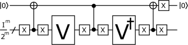
Figure 4: The $(m+1)$-qubit DQC1 model constructed from an $m$-qubit unitary $V$. The line with the slash $/$ means the set of $m$ qubits. A gate acting on this line is applied on each qubit. The first qubit is measured in the computational basis. If the measurement result is 0, as is indicated in the figure, we accept. Otherwise, reject.

VIII.3 Proof of Theorem 4

Given (a description of) a Boolean circuit $f:\{0,1\}^{n}\to\{0,1\}$, we again construct the $(n+\xi)$-qubit unitary operator $U$ such that

$$U(|x\rangle\otimes|0^{\xi}\rangle)=|junk(x)\rangle\otimes|f(x)\rangle$$ (43)

for any $x\in\{0,1\}^{n}$, where $\xi=poly(n)$ and $junk(x)\in\{0,1\}^{n+\xi-1}$ is a bit string. Note that $U$ uses only $X$ and TOFFOLI. Consider the $N^{\prime}\equiv n+\xi+1$ qubit HC1Q circuit in Fig. 5. By a straightforward calculation, the probability of obtaining the result $0^{n}0^{\xi-1}11$, which we define as the acceptance probability $p_{acc}$, is

$$p_{acc}=\frac{gap(f)^{2}}{2^{2n+2\xi}}.$$ (44)

Then, if $gap(f)\neq 0$, $p_{acc}>0$. If $gap(f)=0$, $p_{acc}=0$. The $\xi$-qubit TOFFOLI used in the circuit of Fig. 5 can be decomposed into a linear number of TOFFOLI gates with a single uninitialized ancilla qubit, which can be $|+\rangle$ state Barenco . Therefore, the $N^{\prime}$-qubit HC1Q model is simulated by the $N\equiv N^{\prime}+1=n+\xi+2$ qubit HC1Q model.

Assume that there exists a classical probabilistic algorithm that samples $p_{acc}$ in time $2^{(1-a)n}$ and within a multiplicative error $\epsilon<1$:

$$|p_{acc}-q_{acc}|\leq\epsilon p_{acc},$$ (45)

where $q_{acc}$ is the acceptance probability of the classical algorithm. Then, if $gap(f)\neq 0$,

$$q_{acc}\geq(1-\epsilon)p_{acc}>0,$$ (46)

and if $gap(f)=0$,

$$q_{acc}\leq(1+\epsilon)p_{acc}=0.$$ (47)

This means that deciding $gap(f)\neq 0$ or $gap(f)=0$ can be done in non-deterministic $2^{(1-a)n}$ time, which contradicts to Conjecture 4.

Figure 5: The $(n+\xi+1)$-qubit HC1Q circuit used for the proof. The first line with the slash $/$ means the set of $n$ qubits. The second line with the slash $/$ means the set of $\xi-1$ qubits. A gate acting on these lines is applied on each qubit. All qubits are measured in the computational basis. If the measurement result is $0^{n}0^{\xi-1}11$, as is indicated in the figure, we accept. Otherwise, reject.

VIII.4 Proof of Theorem 2

It is shown in Ref. Cosentino that any logarithmic depth Boolean circuit $f:\{0,1\}^{n}\to\{0,1\}$ (that consists of AND, OR, and NOT) can be implemented with a polynomial-size quantum circuit $U$ acting on $n+1$ qubits such that

$$U(|x\rangle\otimes|b\rangle)=e^{ig(x)}|x\rangle\otimes|f(x)\oplus b\rangle$$ (48)

for all $x\in\{0,1\}^{n}$ and $b\in\{0,1\}$, where $g$ is a certain function. Let us define the $(n+1)$-qubit unitary $V$ by

$$V\equiv(H^{\otimes n}\otimes I)U^{\dagger}(I^{\otimes n}\otimes Z)UH^{\otimes n+1}.$$ (49)

Then,

$$\eta\equiv|\langle 0^{n+1}|V|0^{n+1}\rangle|^{2}=\frac{gap(f)^{2}}{2^{2n+1}}.$$ (50)

From now on the same proof holds as the proof of Theorem 1 with $\xi=1$. Therefore, we can construct the $N$-qubit DQC1 model with $N=n+3$ such that its acceptance probability $p_{acc}$ satisfies $p_{acc}>0$ when $gap(f)\neq 0$, and $p_{acc}=0$ when $gap(f)=0$. If $p_{acc}$ is classically sampled within a multiplicative error $\epsilon<1$ in $2^{(1-a)(N-3)}=2^{(1-a)n}$-time, Conjecture 5 is violated.

VIII.5 Proof of Theorem 3

For a given polynomial-size classical reversible circuit $C:\{0,1\}^{n+\xi}\to\{0,1\}^{n+\xi}$ that consists of only NOT and TOFFOLI, its quantum version, $U$, works as

$$U(|x\rangle\otimes|0^{\xi}\rangle)=|junk(x)\rangle\otimes|C_{n+\xi}(x0^{\xi})\rangle$$ (51)

for any $x\in\{0,1\}^{n}$, where $junk(x)\in\{0,1\}^{n+\xi-1}$ is a bit string (it is actually the first $n+\xi-1$ bits of $C(x0^{\xi})$.) Therefore, the same proof as that of Theorem 1 holds by considering $C_{n+\xi}(x0^{\xi})$ as $f(x)$. Hence we can construct the $N$-qubit DQC1 model with $N=n+\xi+2$ whose acceptance probability cannot be classically sampled within a multiplicative error $\epsilon<1$ in $2^{(1-a)(N-\xi-2)}=2^{(1-a)n}$-time.

VIII.6 Proof of Theorem 5

It is the same as the proof of Theorem 4 by replacing $f(x)$ with $C_{n+\xi}(x0^{\xi})$.

VIII.7 Proof of Theorem 6

For a given 3-CNF with $m$ clauses, $f:\{0,1\}^{n}\to\{0,1\}$, let us construct the unitary operator $U$ such that

$$U(|x\rangle\otimes|0^{\xi}\rangle)=|junk(x)\rangle\otimes|f(x)\rangle$$ (52)

for any $x\in\{0,1\}^{n}$, where $junk(x)\in\{0,1\}^{n+\xi-1}$ is a certain bit string, and $U$ consists of only NOT and TOFFOLI. Such $U$ is constructed by replacing each AND and OR in $f$ with TOFFOLI. The 3-CNF $f$ contains $2m$ OR gates and $m-1$ AND gates. The replacement of a single AND (or OR) gate with TOFFOLI needs a single ancilla qubit initialized to 0, and therefore

$$\xi=2m+m-1=3m-1.$$ (53)

Let us define the circuit $V$ by

$$V\equiv(H^{\otimes n+\xi-1}\otimes X)U(H^{\otimes n}\otimes I^{\otimes\xi}).$$ (54)

Then

$$p_{acc} \equiv |\langle 0^{n+\xi}|V|0^{n+\xi}\rangle|^{2}$$ (55)

$$= |\langle+^{n+\xi-1}1|\frac{1}{\sqrt{2^{n}}}\sum_{x\in\{0,1\}^{n}}|junk(x)\rangle\otimes|f(x)\rangle|^{2}$$

$$= \frac{(\#f)^{2}}{2^{2n+\xi-1}}.$$

The circuit $V$ has $3m-1$ TOFFOLI gates. A single TOFFOLI gate can be represented by Clifford gates and seven $T$ gates NC . Therefore $V$ has $t=21m-7$ $T$ gates, which means $m=\frac{t+7}{21}$. Assume that $p_{acc}$ is calculated within an additive error smaller than $2^{-\frac{3t+14}{7}}$ and in $2^{o(t)}$ time. Then, since

$$\frac{1}{2^{\frac{3t+14}{7}}}\leq\frac{1}{2}\times\frac{1}{2^{2n+\xi-1}}$$ (56)

(note that $n\leq 3m$), and

$$2^{o(t)}=2^{o(\frac{t+7}{21})}=2^{o(m)},$$ (57)

it means that $\#f>0$ or $\#f=0$ can be decided in $2^{o(m)}$ time, which contradicts to Conjecture 1.

VIII.8 Proof of Theorem 7

For a given 3-CNF with $m$ clauses, $f:\{0,1\}^{n}\to\{0,1\}$, let us construct the same unitary operator $U$ such that

$$U(|x\rangle\otimes|0^{\xi}\rangle)=|junk(x)\rangle\otimes|f(x)\rangle$$ (58)

for any $x\in\{0,1\}^{n}$, where $junk(x)\in\{0,1\}^{n+\xi-1}$ is a certain bit string, $U$ consists of only NOT and TOFFOLI, and $\xi=3m-1$. Let us define the circuit $V$ by

$$V\equiv H^{\otimes n+\xi}(I^{\otimes n+\xi-1}\otimes Z)U(H^{\otimes n}\otimes I^{\otimes\xi}).$$ (59)

Then

$$p_{acc}\equiv|\langle 0^{n+\xi}|V|0^{n+\xi}\rangle|^{2}=\frac{gap(f)^{2}}{2^{2n+\xi}}.$$ (60)

Since $V$ has $t=21m-7$ $T$ gates, if $p_{acc}$ can be classically sampled within a multiplicative error $\epsilon<1$ in $2^{o(t)}$ time, it means $gap(f)\neq 0$ or $gap(f)=0$ is decided in non-deterministic $2^{o(m)}$ time, which contradicts to Conjecture 7.

VIII.9 Proof of Theorem 8

It was shown in Ref. BravyiSmithSmolin that any quantum circuit over Clifford gates and $t$ $T$ gates can be simulated by a $t$-qubit PBC. Therefore, the acceptance probability $p_{acc}$ of Eq. (60) can be exactly sampled with a $t=21m-7$ qubit PBC. Due to Conjecture 7, $p_{acc}$ cannot be classically sampled within a multiplicative error $\epsilon<1$ and time $2^{o(m)}=2^{o(t)}$.

VIII.10 Proof of Theorem 9

Given a polynomial-size Boolean circuit $f:\{0,1\}^{n}\to\{0,1\}$, construct the unitary $U$ that consists of only NOT and TOFFOLI such that

$$U(|x\rangle\otimes|0^{\xi}\rangle)=|junk(x)\rangle\otimes|f(x)\rangle$$ (61)

for any $x\in\{0,1\}^{n}$ by replacing each AND and OR of $f$ with TOFFOLI, where $\xi=poly(n)$ is the number of AND and OR gates in $f$ and $junk(x)\in\{0,1\}^{n+\xi-1}$ is a certain bit string. From $U$, we can construct $V$ such that

$$V(|x\rangle\otimes|0^{\xi}\rangle\otimes|0\rangle)=|x\rangle\otimes|0^{\xi}\rangle\otimes|f(x)\rangle$$ (62)

for any $x\in\{0,1\}^{n}$. In fact, with a CNOT gate, we can copy the value of $f(x)$ to an additional ancilla qubit as

$$|junk(x)\rangle\otimes|f(x)\rangle\otimes|0\rangle$$ (63)

$$\to |junk(x)\rangle\otimes|f(x)\rangle\otimes|f(x)\rangle.$$

We then apply $U^{\dagger}$ so that

$$U^{\dagger}(|junk(x)\rangle\otimes|f(x)\rangle)\otimes|f(x)\rangle$$ (64)

$$= |x\rangle\otimes|0^{\xi}\rangle\otimes|f(x)\rangle.$$

Then if we define $W$ by

$$W\equiv(H^{\otimes n}\otimes I^{\otimes\xi}\otimes H)V(H^{\otimes n}\otimes I^{\otimes\xi+1}),$$ (65)

we obtain

$$|\langle 0^{n+\xi}1|W|0^{n+\xi+1}\rangle|^{2}=\frac{gap(f)^{2}}{2^{2n+1}},$$ (66)

which cannot be classically sampled within a multiplicative error $\epsilon<1$ in $2^{(1-a)n}=2^{(1-a)(\frac{h}{2}-\frac{1}{2})}$ time, where $h\equiv 2n+1$ is the number of $H$ in $W$.

VIII.11 Proof of Theorem 10

Given a CNF, $f:\{0,1\}^{h}\to\{0,1\}$, with at most $ch$ clauses, let us construct the $N\equiv h+\xi+1$ qubit quantum circuit $U$ such that

$$U(|x\rangle\otimes|0^{\xi}\rangle\otimes|0\rangle)=|x\rangle\otimes|0^{\xi}\rangle\otimes|f(x)\rangle$$ (67)

for any $x\in\{0,1\}^{h}$. Such $U$ is constructed by replacing AND and OR of $f$ with TOFFOLI. Therefore $U$ consists of $X$, CNOT, and TOFFOLI. The CNF $f$ contains at most $ch(2h-1)$ OR gates and $ch-1$ AND gates. Therefore, $\xi=ch(2h-1)+ch-1=2ch^{2}-1$. If we define the $N$-qubit quantum circuit $V$ by

$$V\equiv U(H^{\otimes h}\otimes I^{\otimes\xi+1}),$$ (68)

then,

$$\|(I^{\otimes N-1}\otimes|1\rangle\langle 1|)V|0^{N}\rangle\|^{2}=\frac{\#f}{2^{h}}.$$ (69)

If it is exactly classically calculated in deterministic $2^{(1-a)h}$ time, we can decide $\#f>0$ or $\#f=0$ in deterministic $2^{(1-a)h}$ time, which violates SETH.

VIII.12 Proof of Theorem 11

By using a similar construction as that in Ref. Dawson , for any $a,b\in\{0,1\}^{N}$, $\langle a|U|b\rangle$ can be written as

$$\langle a|U|b\rangle=\frac{1}{\sqrt{2^{h}}}\sum_{x\in\{0,1\}^{h}}(e^{i\frac{\pi}{4}})^{f_{1}(x)}(-1)^{f_{2}(x)},$$ (70)

where $h$ is the number of $H$ gates in $U$,

$$f_{1}(x)=\sum_{i=1}^{h}\alpha_{i}x_{i}+\beta$$ (71)

with $\alpha_{i},\beta\in\{1,2,3,4,5,6,7\}$, and

$$f_{2}(x)=\sum_{i=1}^{h}\sum_{j=1}^{h}\gamma_{i,j}x_{i}x_{j}+\delta$$ (72)

with $\gamma_{i,j},\delta\in\{0,1\}$.

For a degree $2$ polynomial $p\in\mathbb{Z}[x_{1},x_{2},\ldots,x_{h}]$ and an integer $j\in\{0,1,\ldots,7\}$, we define a Boolean function $g_{j}:\{0,1\}^{h}\to\{0,1\}$ as

$$g_{j}(x)=\begin{cases}1&\text{if $p(x)\equiv j\bmod 8$,}\\ 0&\text{otherwise.}\end{cases}$$

We have

$$\sum_{x\in\{0,1\}^{h}}(e^{i\frac{\pi}{4}})^{p(x)} = \sum_{x\in\{0,1\}^{h}}\sum_{j=0}^{7}(e^{i\frac{\pi}{4}})^{j}g_{j}(x)$$ (73)

$$= \sum_{j=0}^{7}(e^{i\frac{\pi}{4}})^{j}\sum_{x\in\{0,1\}^{h}}g_{j}(x).$$ (74)

We will show that for some $a<1$ and any $j$, $\sum_{x\in\{0,1\}^{h}}g_{j}(x)$ can be computed in deterministic time $2^{ah+o(h)}$. First we represent $g_{j}$ as a polynomial in $\mathbb{Z}_{2}[x_{1},x_{2},\ldots,x_{h}]$.

Fact 1

For each $j\in\{0,1,\ldots,7\}$, there exists a degree $14$ polynomial $p_{j}\in\mathbb{Z}[x_{1},x_{2},\ldots,x_{h}]$ such that $g_{j}(x)\equiv p_{j}(x)\bmod 2$ holds for all $x\in\{0,1\}^{h}$.

Proof. The fact is an immediate consequence of the following.

Lemma 4 (see e.g. BeigelT94 ; ChandraSV84 )

There is a degree $7$ polynomial $q\in\mathbb{Z}[x]$ such that

$$q(x)=\begin{cases}1&\text{if $x\equiv 0\bmod 8$,}\\ 0&\text{otherwise,}\end{cases}$$

holds for all $x\in\mathbb{Z}$.

Setting $p_{j}(x)=q(p(x)-j)$ completes the proof.

At this point, computing $\sum_{x\in\{0,1\}^{h}}g_{j}(x)$ is reduced to counting the number of roots of the equation $p_{j}(x)\equiv 1\bmod 2$. To do so, we will follow the approach of Lokshtanov et al. Tamaki . We make use of $k$-modulus amplifying polynomials given by the following lemma.

Lemma 5 (BeigelT94 )

For all positive integer $k$, there is a degree $2k-1$ polynomial $r_{k}\in\mathbb{Z}[x]$ such that for all $x\in\mathbb{Z}$, it holds that

$$\begin{array}[]{lll}x\equiv 0\bmod 2&\Rightarrow&r_{k}(x)\equiv 0\bmod 2^{k},\\ x\equiv 1\bmod 2&\Rightarrow&r_{k}(x)\equiv 1\bmod 2^{k}.\end{array}$$

For a positive integer $k$ and an integer $j\in\{0,1,\ldots,7\}$, let

$$s_{j,k}(y)=\sum_{z\in\{0,1\}^{k}}r_{k+1}(p_{j}(y_{1},\ldots,y_{h-k},z_{1},\ldots,z_{k})).$$

Then we have:

Fact 2

For all $y\in\{0,1\}^{h-k}$,

$$\sum_{z\in\{0,1\}^{k}}g_{j}(y_{1},\ldots,y_{h-k},z_{1},\ldots,z_{k})\equiv s_{j,k}(y)\bmod 2^{k+1}.$$

Since $r_{k+1}(p_{j}(y_{1},\ldots,y_{h-k},z_{1},\ldots,z_{k}))$ is a multi-linear polynomial of degree $14(2k+1)$, we can write it down as a sum of terms in time

$$\binom{h-k}{14(2k+1)}2^{o(h)}.$$

for each $z\in\{0,1\}^{k}$. Thus, we can write down $s_{j,k}(y)$ as a sum of terms in time

$$\binom{h-k}{14(2k+1)}2^{k+o(h)}.$$

Then, we apply the following lemma.

Lemma 6 (see e.g. Section 6.2 in Williams11 )

Given a multi-linear polynomial $p\in\mathbb{Z}[x_{1},\ldots,x_{h}]$ represented as a sum of terms, we can obtain the evaluation of $p$ for all $x\in\{0,1\}^{h}$ in time $2^{h+o(h)}$.

The lemma implies that we can obtain the evaluation of $s_{j,k}(y)$ for all $y\in\{0,1\}^{h-k}$ in time $2^{h-k+o(h)}$. By Fact 2, we also obtain the evaluation of

$$t_{j}(y)=\sum_{z\in\{0,1\}^{k}}g_{j}(y_{1},\ldots,y_{h-k},z_{1},\ldots,z_{k})$$ (75)

for all $y$. Finally we obtain the value of $\sum_{x\in\{0,1\}^{h}}g_{j}(x)$ by calculating $\sum_{y\in\{0,1\}^{h-k}}t_{j}(y)$ in time $2^{h-k+o(h)}$.

In the above procedure, required computation time is at most

$$\binom{h-k}{14(2k+1)}2^{k+o(h)}+2^{h-k+o(h)}.$$

By setting $k=h\times 0.015035\cdots$, both terms are bounded above by $2^{0.984965h+o(h)}$.

VIII.13 Proof of Lemma 2

Assume that a language $L$ is in coNP. Then, if $x\in L$ then $\#f=0$, and if $x\notin L$ then $\#f>0$, where $f$ is a certain Boolean circuit. By the assumption, we can construct the quantum circuit $V$. Then, if $x\in L$ then $p_{acc}>0$, and if $x\notin L$ then $p_{acc}=0$. This means that coNP is in ${\rm NQP}_{\rm DQC1}$, where ${\rm NQP}_{\rm DQC1}$ is equivalent to NQP except that the decision quantum circuit is the DQC1 model. Here NQP is a quantum version of NP, and defined as follows.

Definition 10

A language $L$ is in NQP if and only if there exists a uniformly-generated family $\{V_{x}\}_{x}$ of polynomial-size quantum circuits such that if $x\in L$ then $p_{acc}>0$ and if $x\notin L$ then $p_{acc}=0$, where $p_{acc}$ is the acceptance probability of $V_{x}$.

It is known that ${\rm NQP}={\rm NQP}_{\rm DQC1}$ Kobayashi ; KobayashiICALP , and therefore we have shown ${\rm coNP}\subseteq{\rm NQP}={\rm coC}_{=}{\rm P}$.

VIII.14 Proof of Theorem 12

For a given 3-CNF with $m$ clauses, $f:\{0,1\}^{n}\to\{0,1\}$, let us construct the $(n+\xi+1)$-qubit unitary $U$ such that

$$U(|x\rangle\otimes|0^{\xi}\rangle\otimes|0\rangle)=|x\rangle\otimes|0^{\xi}\rangle\otimes|f(x)\rangle$$ (76)

for any $x\in\{0,1\}^{n}$, where $\xi=3m-1$. Such $U$ is constructed as follows. First, we replace each AND and OR in $f$ with a single TOFFOLI by adding a single ancilla bit initialized to 0. Since $f$ contains $2m$ OR gates and $m-1$ AND gates, the number of TOFFOLI gates (and the number of ancilla bits) is $\xi=2m+m-1=3m-1$. Let $U^{\prime}$ be thus constructed circuit. The circuit $U^{\prime}$ contains NOT gates and $\xi$ TOFFOLI gates. If we consider it as a quantum unitary circuit,

$$U^{\prime}(|x\rangle\otimes|0^{\xi}\rangle)=|junk(x)\rangle\otimes|f(x)\rangle,$$ (77)

where $junk(x)\in\{0,1\}^{n+\xi-1}$ is a certain bit string whose detail is irrelevant here. Then, we have only to define the $(n+\xi+1)$-qubit unitary $U$ by

$$U\equiv((U^{\prime})^{-1}\otimes H)(I^{\otimes n+\xi-1}\otimes CZ)(U^{\prime}\otimes H).$$ (78)

From the construction, it is clear that $U$ consists of only $X$, CNOT, and TOFFOLI gates. Let us define the $(n+\xi+1)$-qubit quantum circuit $V$ by

$$V\equiv(H^{\otimes n}\otimes I^{\otimes\xi}\otimes X)U(H^{\otimes n}\otimes I^{\otimes\xi+1}).$$ (79)

Then,

$$\langle 0^{n+\xi+1}|V|0^{n+\xi+1}\rangle=\frac{\#f}{2^{n}}.$$ (80)

Let $|\Psi\rangle$ be a resource of $\xi$ TOFFOLI gates. Then there exists an $(n+\xi+1+r)$-qubit Clifford circuit $W$ such that

$$\langle 0^{n+\xi+1}|V|0^{n+\xi+1}\rangle$$ (81)

$$= \eta^{-1}\langle 0^{n+\xi+1+r}|W(|0^{n+\xi+1}\rangle\otimes|\Psi\rangle)$$

$$= \sum_{j=1}^{\chi(|\Psi\rangle)}\eta^{-1}c_{j}\langle 0^{n+\xi+1+r}|W(|0^{n+\xi+1}\rangle\otimes C_{j}|0^{r}\rangle),$$

where

$$\eta\equiv\Big{\|}(I^{\otimes n+\xi+1}\otimes|0^{r}\rangle\langle 0^{r}|)|W\Big{(}|0^{n+\xi+1}\rangle\otimes|\Psi\rangle\Big{)}\Big{\|}.$$ (82)

The quantity of Eq. (81) can be computed in $\chi(|\Psi\rangle)\times poly(\xi,n)$ time, and therefore

$$\chi(|\Psi\rangle)\times poly(\xi,n)\geq 2^{\Omega(m)},$$ (83)

which means

$$\chi(|\Psi\rangle)\geq\frac{2^{\Omega(\xi)}}{poly(\xi,n)}\geq\frac{2^{\Omega(\xi)}}{poly(\xi)}=2^{\Omega(\xi)},$$ (84)

where we have used $n\leq 3m=\xi+1$.

- (1) H. Buhrman, R. Cleve, and A. Wigderson, Quantum vs. classical communication and computation. Proceedings of the 30th Annual ACM Symposium on Theory of Computing, p.63 (1998).
- (2) R. Raz, Exponential separation of quantum and classical communication complexity. Proceedings of the 31st Annual ACM Symposium on Theory of Computing, p.358 (1999).
- (3) H. Buhrman, R. Cleve, S. Massar, and R. de Wolf, Nonlocality and communication complexity. Rev. Mod. Phys. 82, 665 (2010).
- (4) H. Buhrman, R. Cleve, J. Watrous, and R. de Wolf, Quantum fingerprinting. Phys. Rev. Lett. 87, 167902 (2001).
- (5) BQP is the class of decision problems that are efficiently solved with a quantum computer. BPP is the class of decision problems that are efficiently solved with a classical probabilistic computer. Therefore, “quantum computing is faster than classical computing” means . P is the class of decision problems that are efficiently solved with a classical deterministic computer. PSPACE is the class of decision problems that are solved with a memory-efficient classical deterministic computer. It is known that . Therefore, if we can show , we can show , but it is one of the long-standing open problems in classical complexity theory. It therefore suggests that showing will not be easy. For detailed definitions of complexity classes, see the complexity zoo. https://complexityzoo.uwaterloo.ca/Complexity_Zoo
- (6) P. W. Shor, Algorithms for quantum computation: discrete logarithms and factoring. Proceedings of the 35th Annual Symposium on Foundations of Computer Science (FOCS 1994), p.124 (1994).
- (7) I. M. Georgescu, S. Ashhab, and F. Nori, Quantum simulation. Rev. Mod. Phys. 86, 153 (2014).
- (8) E. Tang, A quantum-inspired classical algorithm for recommendation systems, arXiv:1807.04271
- (9) L. K. Grover, Quantum mechanics helps in searching for a needle in haystack. Phys. Rev. Lett. 79, 325 (1997).
- (10) D. R. Simon, On the power of quantum computation. Proceedings of the 35th Annual Symposium on Foundations of Computer Science (FOCS 1994), p.116 (1994).
- (11) B. M. Terhal and D. P. DiVincenzo, Adaptive quantum computation, constant depth quantum circuits and Arthur-Merlin games. Quant. Inf. Comput. 4, 134 (2004).
- (12) S. Aaronson and A. Arkhipov, The computational complexity of linear optics. Theory of Computing 9, 143 (2013).
- (13) M. J. Bremner, R. Jozsa, and D. J. Shepherd, Classical simulation of commuting quantum computations implies collapse of the polynomial hierarchy. Proc. R. Soc. A 467, 459 (2011).
- (14) M. J. Bremner, A. Montanaro, and D. J. Shepherd, Average-case complexity versus approximate simulation of commuting quantum computations. Phys. Rev. Lett. 117, 080501 (2016).
- (15) E. Knill and R. Laflamme, Power of one bit of quantum information. Phys. Rev. Lett. 81, 5672 (1998).
- (16) T. Morimae, K. Fujii, and J. F. Fitzsimons, Hardness of classically simulating the one clean qubit model. Phys. Rev. Lett. 112, 130502 (2014).
- (17) T. Morimae, Hardness of classically sampling one clean qubit model with constant total variation distance error. Phys. Rev. A 96, 040302(R) (2017).
- (18) K. Fujii, H. Kobayashi, T. Morimae, H. Nishimura, S. Tamate, and S. Tani, Impossibility of classically simulating one-clean-qubit model with multiplicative error. Phys. Rev. Lett. 120, 200502 (2018).
- (19) K. Fujii, H. Kobayashi, T. Morimae, H. Nishimura, S. Tamate, and S. Tani, Power of quantum computation with few clean qubits. Proceedings of 43rd International Colloquium on Automata, Languages, and Programming (ICALP 2016), pp.13:1-13:14 (2016).
- (20) A. Bouland, B. Fefferman, C. Nirkhe, and U. Vazirani, Quantum supremacy and the complexity of random circuit sampling. arXiv:1803.04402
- (21) R. Movassagh, Efficient unitary paths and quantum computational supremacy: A proof of average-case hardness of Random Circuit Sampling. arXiv:1810.04681
- (22) R. Movassagh, Cayley path and quantum computational supremacy: A proof of average-case -hardness of Random Circuit Sampling with quantified robustness. arXiv:1909.06210
- (23) T. Morimae, Y. Takeuchi, and H. Nishimura, Merlin-Arthur with efficient quantum Merlin and quantum supremacy for the second level of the Fourier hierarchy. Quantum 2, 106 (2018).
- (24) V. Vassilevska Williams, Hardness of easy problems: Basing hardness on popular conjectures such as the strong exponential time hypothesis. In Proc. International Symposium on Parameterized and Exact Computation, pages 16-28 (2015).
- (25) A. M. Dalzell, A. W. Harrow, D. E. Koh, and R. L. La Placa, How many qubits are needed for quantum computational supremacy? arXiv:1805.05224
- (26) A. M. Dalzell, Bachelor thesis, MIT (2017). https://dspace.mit.edu/handle/1721.1/111859
- (27) C. Huang, M. Newman, and M. Szegedy, Explicit lower bounds on strong quantum simulation. arXiv:1804.10368
- (28) C. Huang, M. Newman, and M. Szegedy, Explicit lower bounds on strong simulation of quantum circuits in terms of -gate count. arXiv:1902.04764
- (29) R. Impagliazzo, R. Paturi, and F. Zane, Which problems have strongly exponential complexity? J. Comput. Syst. Sci. 63(4), 512-530 (2001).
- (30) R. Impagliazzo and R. Paturi, On the complexity of k-SAT. J. Comput. Syst. Sci. 62(2), 367-375 (2001).
- (31) M. L. Carmosino, J. Gao, R. Impagliazzo, I. Mihajlin, R. Paturi, S. Schneider, Nondeterministic Extensions of the Strong Exponential Time Hypothesis and Consequences for Non-reducibility. ITCS 2016: 261-270
- (32) T. M. Chan and R. Williams, Deterministic APSP, Orthogonal Vectors, and More: Quickly Derandomizing Razborov-Smolensky. SODA 2016: 1246-1255.
- (33) A. Abboud, T. D. Hansen, V. V. Williams, and R. Williams, Simulating branching programs with edit distance and friends: or: a polylog shaved is a lower bound made. STOC 2016: 375-388.
- (34) D. Poulin, R. Laflamme, G. J. Milburn, and J. P. Paz, Testing integrability with a single bit of quantum information. Phys. Rev. A 68, 022302 (2003).
- (35) D. Poulin, R. Blume-Kohout, R. Laflamme, and H. Ollivier, Exponential speedup with a single bit of quantum information: measuring the average fidelity decay. Phys. Rev. Lett. 92, 177906 (2004).
- (36) G. Passante, O. Moussa, C. A. Ryan, and R. Laflamme, Experimental approximation of the Jones polynomial with one quantum bit. Phys. Rev. Lett. 103, 250501 (2009).
- (37) P. W. Shor and S. P. Jordan, Estimating Jones polynomials is a complete problem for one clean qubit. Quant. Inf. Comput. 8, 681 (2008).
- (38) S. P. Jordan and P. Wocjan, Estimating Jones and HOMFLY polynomials with one clean qubit. Quat. Inf. Comput. 9, 264 (2009).
- (39) S. P. Jordan and G. Alagic, Approximating the Turaev-Viro invariant of mapping tori is complete for one clean qubit. arXiv:1105.5100
- (40) T. Morimae, K. Fujii, and H. Nishimura, Power of one non-clean qubit. Phys. Rev. A 95, 042336 (2017).
- (41) Y. Shi, Quantum and classical tradeoffs. Theoretical Computer Science 344, 335 (2005).
- (42) D. Gottesman, The Heisenberg representation of quantum computers. arXiv:quant-ph/9807006
- (43) L. G. Valiant, Quantum computers that can be simulated classically in polynomial time. Proceedings of the 33rd Annual ACM Symposium on Theory of Computing p.114 (2001).
- (44) S. Bravyi and D. Gosset, Improved classical simulation of quantum circuits dominated by Clifford gates. Phys. Rev.Lett. 116, 250501 (2016).
- (45) S. Bravyi, G. Smith, and J. A. Smolin, Trading classical and quantum computational resources. Phys. Rev. X 6, 021043 (2016).
- (46) D. Lokshtanov, R. Paturi, S. Tamaki, R. Williams, and H. Yu, Beating brute force for systems of polynomial equations over finite fields. Proceedings of the 28th Annual ACM-SIAM Symposium on Discrete Algorithms, pp.2190-2202 (2017).
- (47) R. Beigel, Relativized counting classes: Relations among thresholds, parity, and Mods. J. of Comput. System. Sci. 42, 76 (1991).
- (48) M. Cygan et al., On problems as hard as CNF-SAT. ACM Transactions on Algorithms 12, 41 (2016).
- (49) A. Gajentaan and M. Overmars, On a class of problems in computational geometry. Computational Geometry 5, 165-185 (1995).
- (50) L. Roditty and U. Zwick, On dynamic shortest paths problems. In Algorithms ESA 2004, 12th Annual European Symposium, Bergen, Norway, September 14-17, 2004, Proceedings, pages 580-591, 2004.
- (51) Note that for the additive error supremacy, all output qubits have to be measured.
- (52) M. Ball, A. Rosen, M. Sabin, and P. N. Vasudevan, Average-case fine-grained hardness. Proceedings of the 49th Annual ACM SIGACT Symposium on Theory of Computing (STOC 2017), pages 483-496.
- (53) A. Barenco et al., Elementary gates for quantum computation. Phys. Rev. A 52, 3457 (1995).
- (54) A. Cosentino, R. Kothari, and A. Paetznick, Dequantizing read-once quantum formulas. TQC 2013.
- (55) R. Beigel and J. Tarui, On ACC. Computational Complexity 4, 350-366 (1994).
- (56) A. K. Chandra, L. J. Stockmeyer, and U. Vishkin, Constant depth reducibility. SIAM J. Comput. 13, 423-439 (1984).
- (57) R. Williams, A casual tour around a circuit complexity bound. SIGACT News 42, 54-76 (2011).
- (58) M. A. Nielsen and I. L. Chuang, Quantum Computation and Quantum Information (Cambridge University Press, Cambridge, UK, 2002).
- (59) A. Datta, S. T. Flammia, and C. M. Caves, Entanglement and the power of one qubit. Phys. Rev. A 72, 042316 (2005).
- (60) C. M. Dawson, H. L. Haselgrove, A. P. Hines, D. Mortimer, M. A. Nielsen, and T. J. Osborne, Quatnum computing and polynomial equations over the finite field . Quant. Inf. Comput. 5, 102 (2005).