Perturbation calculations on interlayer transmission rates from symmetric to antisymmetric channels in parallel armchair nanotube junctions

Abstract

Partially overlapping two parallel armchair nanotubes are investigated theoretically with the $\pi$ orbital tight bonding model. Considering the interlayer Hamiltonian as perturbation, we obtain approximate analytical formulas of the interlayer transmission rates $T_{\sigma^{\prime},\sigma}$ from channel $\sigma$ to $\sigma^{\prime}$ for all the four combinations $(\sigma^{\prime},\sigma)=(\pm,\pm)$ and $(\pm,\mp)$, where suffixes $+$ and $-$ represent symmetric and antisymmetric channels, respectively, with respect to the mirror plane of each tube. Landauer’s formula conductance is equal to the sum of them in units of $2e^{2}/h$. According to the perturbation calculation, the interlayer Hamiltonian is transformed into the parameter $w_{\sigma^{\prime},\sigma}$ that determines the analytical formula of $T_{\sigma^{\prime},\sigma}$. By comparison with the exact numerical results, the effective range of the analytical formulas is discussed. In the telescoped coaxial contact, the off-diagonal part $T_{-,+}+T_{+,-}$ is very small compared to the diagonal part $T_{+,+}+T_{-,-}$. In the side contact, on the other hand, the off-diagonal part is more significant than the diagonal part in the zero energy peak of the conductance.

I introduction

In the growing area of carbon nanotubes (NT) [1, 2] and graphenes (GR) [3], interlayer interaction has important roles. In the NT system, it brings about pseudogaps [4], nearly free electron states [5], and formation of single wall NT ropes [6]. In the multi-layer GR, it causes band gaps under the electric field [7], and superconductivity of twisted bilayer GR [8]. The two inequivalent Fermi points K and K’ of the single layer are called valleys. Effective mass theory shows that a boundary between monolayer and bilayer GR works as valley current filters [9]. Since interlayer bonds are much weaker than intralayer bonds, interlayer sliding and rotation occur keeping the honeycomb lattice. Telescopic extension of multiwall NTs has been investigated experimentally [10] and theoretically [11] as GHz oscillators and nano springs. Interlayer interaction energy and force were calculated for a stack of GR flakes [12] and for a NT on a GR layer [13]. Molecular dynamic calculations indicate that AB stacking is the most stable in the NT-GR connection [14]. The interlayer force is usually classified to van der Waals force caused by virtual dipole-dipole interaction that could exist without the interlayer orbital overlap [15]. The electronic structures, however, are described well by the tight binding (TB) model with the interlayer transfer integrals that originate from the interlayer orbital overlap [16]. In the present paper, the interlayer transfer integral is termed the interlayer bond. Interlayer ’covalent’ bonds induced by beam irradiation, heating and defects [17] are excluded in our discussion as they hinder the nearly free interlayer motion.

Among various multi-layer systems, a single layer $\downarrow$ partially overlapping with another single layer $\uparrow$ is outstanding in the relation between the interlayer bonds and the conductance. It is represented by (L,$\downarrow$)-(D,$\downarrow$,$\uparrow$)-(R,$\uparrow$) where interlayer bonds are limited to the overlapped region D. Connecting the source and drain electrodes to single layer regions L and R, respectively, we can force the net current to flow through the interlayer bonds. In contrast to this $\downarrow$-$\uparrow$ junction, the net current between $\downarrow$ and $\uparrow$ is zero in the junctions (L,$\downarrow$)-(D,$\downarrow$,$\uparrow$)-(R,$\downarrow$) where both the source and drain electrodes are connected to $\downarrow$ [18]. The $\downarrow$-$\uparrow$ conductance was measured for the telescoped NTs [19]. The Landauer’s formula conductance of $\downarrow$-$\uparrow$ junctions has been reported. The combinations $\downarrow$- $\uparrow$ are GR-GR [20], NT-GR [21] and NT-NT. Telescoped coaxial contacts [22, 23, 24, 25, 26] and side contacts [27, 28] were discussed for the NT-NT junctions. Comparisons between the two contacts were also reported [29, 30].

The Landauer’s formula conductance is the sum of the interlayer transmission rates $T_{\sigma^{\prime},\sigma}$ of which indexes $\sigma^{\prime}$ and $\sigma$ denote channels of R and L, respectively. Wave numbers $k_{1}$ and $k_{2}$ of region D appear in the dependence of $T_{\sigma^{\prime},\sigma}$ on the overlapped length as the periods of the beating, $2\pi/|k_{1}-k_{2}|$ and $2\pi/|k_{1}+k_{2}|$. In addition to this $(k_{1},k_{2})$ characteristic, we can show that $T_{\sigma^{\prime},\sigma}$ is proportional to $|W|^{2}$ considering the interlayer bond $W$ as perturbation [23, 26, 30]. It is termed the $|W|^{2}$ characteristic here. The $(k_{1},k_{2})$ and $|W|^{2}$ characteristics appear in the period and in the amplitude of the oscillation, respectively, while both originate from $W$. Whereas the numerical calculation method about $T_{\sigma^{\prime},\sigma}$ has been established [31], it does not diminish the value of the perturbation calculation producing analytical formulas. Without the perturbation calculation, one might assume an analytical formula of which fitting parameters are optimized for the coincidence with the numerical results. In this fitting method, however, the fear is that choice of the formula may become arbitrary. When we know the exact eigen states of the unperturbed Hamiltonian, however, we can derive the unique perturbation expansion [15].

In the present paper, $\downarrow$ and $\uparrow$ are chosen to be parallel $(n_{\downarrow},n_{\downarrow})$ and $(n_{\uparrow},n_{\uparrow})$ armchair NTs, because their mirror symmetry and small unit cell enable us to perform the analytical perturbation calculation. Figure 1 shows the (a) side contact and (b) telescoped coaxial contact. The mirror symmetry of each NT is indicated by $\sigma=+$ and $\sigma=-$ in the suffixes of $T_{\sigma^{\prime},\sigma}$. The $(k_{1},k_{2})$ characteristic does not appear in the nonparallel crossed NT junction without periodicity in region D [32]. In the chiral NT junctions, the large unit cell of region D makes the $(k_{1},k_{2})$ characteristic complicated [26, 30]. In the reported theoretical works on the $(n_{\uparrow},n_{\uparrow})$-$(n_{\downarrow},n_{\downarrow})$ junctions, the diagonal transmission rates $T_{+,+}$ and $T_{-,-}$ and the sum $\sum_{\sigma}\sum_{\sigma^{\prime}}T_{\sigma^{\prime},\sigma}$ have been discussed, but the off-diagonal transmission rates $T_{+,-}$ and $T_{-,+}$ have been neglected. In this paper, we derive the analytical formulas of all four $T_{\sigma^{\prime},\sigma}$ and show how the $|W|^{2}$ and $(k_{1},k_{2})$ characteristics appear there.

II geometrical structure and tight binding model

As is shown by Fig. 1, the tube axis of $\downarrow$ is chosen to be $z$ axis. The atomic $z$ coordinates in tubes $\downarrow$ and $\uparrow$ are $aj/2$ and $aj/2+\Delta z$, respectively, with integers $j$, the lattice constant $a=0.246$ nm and a small translation $|\Delta z|<a/4$. The atomic $y$ coordinates of tube $\xi(=\downarrow,\uparrow)$ are represented by $R_{\xi}\sin\theta^{\xi}_{j,i}$ with the tube radius $R_{\xi}=\frac{\sqrt{3}a}{2\pi}n_{\xi}$. The angles $\theta^{\downarrow}_{j,i}=\frac{\chi_{j,i}}{n_{\downarrow}}$ and $\theta^{\uparrow}_{j,i}=\frac{\chi_{j,i}}{n_{\uparrow}}-\frac{2\pi}{3n_{\uparrow}}+\Delta\theta$ are measured in the opposite direction with positive integers $i$, $\chi_{j,i}\equiv\pi(i-\frac{(-1)^{i}}{6}-\frac{(-1)^{j}}{2})$ and a small rotation $|\Delta\theta|<\pi/n_{\uparrow}$. Thus the atomic $x$ coordinates are $R_{\downarrow}\cos\theta^{\downarrow}_{j,i}$ for tube $\downarrow$, and $D+R_{\uparrow}+R_{\downarrow}-R_{\uparrow}\cos\theta^{\uparrow}_{j,i}$ for tube $\uparrow$. Here $D=$ 0.31 nm is the interlayer distance for the side-contact while $D=-R_{\downarrow}-R_{\uparrow}$ for the coaxial contact. The former is the same as Ref. [29]. When $|n_{\downarrow}-n_{\uparrow}|=5$, the interlayer distance of the coaxial contact is close to that of graphite. For example, Fig. 2 shows the interlayer configuration in the case where $(n_{\downarrow},n_{\uparrow},\Delta\theta,\Delta z)=(10,15,0,0)$. Tubes $\downarrow$ and $\uparrow$ have ’AB’ and ’ab’ sublattices where odd $i$ sites correspond to ’A’ and ’a’ sublattices. In Fig. 2(a) for the side contact, 1A and 1a (2B and 2b) sites correspond to $i=1$ ($i=2$). The interlayer configuration in the side contact is similar to the Ab stacking of the bilayer GR when $(\Delta\theta,\Delta z)=(0,0),(\frac{-2\pi}{3n_{\uparrow}},0)$.

The $\pi$ orbital TB equations with energy $E$ in region D are represented by

$$E\vec{c}_{j}^{\;\rm(D)}=\sum_{\Delta j=-1}^{1}H^{(j,\Delta j)}\vec{c}_{j+\Delta j}^{\;\rm(D)}$$ (1)

where $\;{}^{t}\vec{c}^{\;(\rm D)}_{j}=(\;^{t}\vec{c}^{\;(\rm D,\downarrow)}_{j},\;^{t}\vec{c}^{(\;\rm D,\uparrow)}_{j})$ . The matrix $H^{(j,\Delta j)}$ is partitioned as

$$H^{(j,\Delta j)}=\left(\begin{array}[]{cc}h_{\downarrow}^{(j,\Delta j)},&W^{(j,\Delta j)}\\ \;{}^{t}W^{(j+\Delta j,-\Delta j)},&h_{\uparrow}^{(j,\Delta j)}\end{array}\right).$$ (2)

The blocks $h$ and $W$ correspond to intralayer and interlayer elements, respectively. Figure 3 shows a schematic diagram of the tight binding Hamiltonian. As $H^{(j,\Delta j)}$ is the block of the Hamiltonian matrix partitioned by the half lattice constant $a/2$, $H^{(j+2,\Delta j)}=H^{(j,\Delta j)}$. The $(i,i^{\prime})$ element of $W^{(j,\Delta j)}$ is defined by $t_{1}e^{\frac{d-r}{L_{c}}}\Theta(r-r_{c})|\cos\phi|$ where $\phi=\theta_{j,i}^{\downarrow}+\theta_{j+\Delta j,i^{\prime}}^{\uparrow}$, $t_{1}=$ 0.36 eV, $d=$ 0.334 nm, $L_{c}=$ 0.045 nm, the cut-off radius $r_{c}=0.39$ nm, $r$ denotes the atomic distance and $\Theta$ is the step function defined by $\Theta(x)=1$ for negative $x$ and $\Theta(x)=0$ for positive $x$. The elements between nearest neighbors are $h^{(j,0)}_{\xi,2m-1,2m}$, $h^{(j,0)}_{\xi,2m,2m-1}$, $h^{(1,\pm 1)}_{\xi,2n_{\xi},1}$, $h^{(1,\pm 1)}_{\xi,m-1,m}$, $h^{(2,\pm 1)}_{\xi,1,2n_{\xi}}$ and $h^{(2,\pm 1)}_{\xi,m,m-1}$ with integers $m$. They are equal to the negative constant $-t=-2.75$ eV while the other elements of $h^{(j,\Delta j)}_{\xi}$ are zero. Since $h_{\xi}^{(1,0)}=h_{\xi}^{(2,0)}$ and $h_{\xi}^{(j,1)}=h_{\xi}^{(j,-1)}$, we use the abbreviation $h_{\xi}^{(0)}$ and $h_{\xi}^{(1)}$ in Fig. 3. On the other hand, relations $W^{(1,0)}=W^{(2,0)}$ and $W^{(j,1)}=W^{(j,-1)}$ do not generally hold. The latter relation $W^{(j,1)}=W^{(j,-1)}$ is valid only when $\Delta z=0$.

Our calculation and Refs. [25, 33] are the same in the TB model except that $t_{1}$ has two values 0.36 eV and 0.16 eV in Refs. [25, 33]. As this multivalued $t_{1}$ model was derived from first principle calculation data on multiwall NTs, it may not be effective for the side contact. In our calculation, $t_{1}$ is fixed at the single value 0.36 eV and the geometrical structure is simplified compared to the actual one as a first guess.

III Method of calculation

In order to obtain the transmission rate, we calculate the scattering matrix ($S$ matrix). The $S$ matrix has two useful characteristics. Firstly, unitarity $\;{}^{t}S^{*}=S^{-1}$ is guaranteed by conservation of the probability. When there is time reversal symmetry, $\;{}^{t}S=S$ also holds. These symmetries proved in Appendix A can be used as verification of the obtained results. Secondly, $S$ matrix is directly related to the ratio between incident and scattered wave amplitudes. It leads us to an intuitive formula showing that multiple reflection between the two boundaries causes the transmitted wave.

A exact numerical calculation

Equation (1) enables us to obtain the transfer matrix $\Gamma^{(\rm D)}$ that satisfies $(\;^{t}\vec{c}^{\;(\rm D)}_{2m+1},\;^{t}\vec{c}^{\;(\rm D)}_{2m+2})=(\;^{t}\vec{c}^{\;(\rm D)}_{2m-1},\;^{t}\vec{c}^{\;(\rm D)}_{2m})\;^{t}\Gamma^{(\rm D)}$. Replacing $W^{(j,\Delta j)}$ with zero, we also obtain the transfer matrices $\Gamma^{(\rm L)}$ and $\Gamma^{(\rm R)}$ for regions L and R. With a set of linearly independent eigen vectors $\vec{u}^{\;(\mu)}_{l}$ satisfying $\Gamma^{(\mu)}\vec{u}_{l}^{\;(\mu)}=\lambda_{l}^{(\mu)}\vec{u}_{l}^{\;(\mu)}$ , we can expand $\vec{c}_{j}^{\;(\mu)}$ as

$$\left(\begin{array}[]{c}\vec{c}^{\;(\mu)}_{2m-1}\\ \vec{c}^{\;(\mu)}_{2m}\\ \end{array}\right)=\sum_{l=-2n_{\mu}}^{2n_{\mu}}\vec{u}^{\;(\mu)}_{l}\left(\lambda^{(\mu)}_{l}\right)^{m}\gamma_{l}^{(\mu)}$$ (3)

where $l\neq 0$, $\lambda_{-l}^{(\mu)}=1/\lambda_{l}^{(\mu)}$, $n_{\rm L}=n_{\downarrow},n_{\rm R}=n_{\uparrow}$ and $n_{\rm D}=n_{\rm L}+n_{\rm R}$. The eigen vectors are ordered according to the following rules (i) for propagating waves and (ii) for evanescent waves. Here $\overline{N}_{\mu}$ denotes the channel number of region $\mu$. (i)When $1\leq l\leq\overline{N}_{\mu}$ , $\left|\lambda_{l}^{(\mu)}\right|=1$, $\vec{u}_{-l}^{\;(\mu)}=\left(\vec{u}_{l}^{\;(\mu)}\right)^{*}$ and the probability flow of $\vec{u}_{l}^{\;(\mu)}$ is positive. Note that $|\vec{u}_{l}|^{2}\neq 1$. The normalizatiion of $\vec{u}_{l}^{\;(\mu)}$ is defined by Appendix A. (ii)When $\overline{N}_{\mu}+1\leq l\leq 2n_{\mu}$, $\left|\lambda_{l}^{(\mu)}\right|<1$.

The boundary conditions for the LD junction are

$$\left(\begin{array}[]{c}\vec{c}^{\;(\rm L)}_{j_{\rm l}+1}\\ \vec{c}^{\;(\rm L)}_{j_{\rm l}}\\ 0\end{array}\right)=\left(\begin{array}[]{c}\vec{c}^{\;(\rm D,\downarrow)}_{j_{\rm l}+1}\\ \vec{c}^{\;(\rm D,\downarrow)}_{j_{\rm l}}\\ \vec{c}^{\;(\rm D,\uparrow)}_{j_{\rm l}}\end{array}\right)+\left(\begin{array}[]{c}\frac{1}{h_{\downarrow}^{(j_{\rm l},1)}}W^{(j_{\rm l},1)}\vec{c}^{\;(\rm D,\uparrow)}_{j_{\rm l}+1}\\ 0\\ 0\end{array}\right)$$ (13)

and those of the DR junction are

$$\left(\begin{array}[]{c}\vec{c}^{\;(\rm R)}_{j_{\rm r}}\\ \vec{c}^{\;(\rm R)}_{j_{\rm r}+1}\\ 0\end{array}\right)=\left(\begin{array}[]{c}\vec{c}^{\;(\rm D,\uparrow)}_{j_{\rm r}}\\ \vec{c}^{\;(\rm D,\uparrow)}_{j_{\rm r}+1}\\ \vec{c}^{\;(\rm D,\downarrow)}_{j_{\rm r}+1}\\ \end{array}\right)+\left(\begin{array}[]{c}\frac{1}{h_{\uparrow}^{(j_{\rm r}+1,1)}}\;^{t}W^{(j_{\rm r},1)}\vec{c}^{\;(\rm D,\downarrow)}_{j_{\rm r}}\\ 0\\ 0\end{array}\right)$$ (23)

where $j_{\rm l}$ and $j_{\rm r}$ denote $j$ at the boundaries as is shown by Fig. 1. The geometrical overlapped length equals $z_{\rm R}-z_{\rm L}=-\Delta z+(j_{\rm r}-j_{\rm l}-1)a/2$. Without losing generality, $j_{\rm l}$ is either $-1$ or 0. Derivation of Eqs. (13) and (23) is shown by Appendix B. Since Eq. (3) must not diverge at $j=\pm\infty$, $\gamma_{l}^{(\rm L)}=0$ and $\gamma_{-l^{\prime}}^{(\rm R)}=0$ when $l>\overline{N}_{\rm L}$ and $l^{\prime}>\overline{N}_{\rm R}$. Thus the number of nonzero variables is $M_{\rm var}=2n_{\rm L}+2n_{\rm R}+\overline{N}_{\rm L}+\overline{N}_{\rm R}+4n_{\rm D}$. On the other hand, the number of conditions is $M_{\rm cond}=2n_{\rm L}+2n_{\rm R}+4n_{\rm D}$ to which contributions of Eqs. (13) and (23) are $4n_{\rm L}+2n_{\rm R}$ and $4n_{\rm R}+2n_{\rm L}$ , respectively. Accordingly the number of independent variables is $M_{\rm var}-M_{\rm cond}=\overline{N}_{\rm L}+\overline{N}_{\rm R}$. Choosing $\;{}^{t}\vec{\gamma}_{+}^{\;(\rm L^{\prime})}=(\gamma_{1}^{(\rm L)},\gamma_{2}^{\;(\rm L)},\cdots,\gamma_{\overline{N}_{\rm L}}^{(\rm L)})$ and $\;{}^{t}\vec{\gamma}_{-}^{\;(\rm R^{\prime})}=(\gamma_{-1}^{(\rm R)},\gamma_{-2}^{\;(\rm R)},\cdots,\gamma_{-\overline{N}_{\rm R}}^{(\rm R)})$ for the independent variables, we obtain the scattering matrix $S_{\rm RL}$ satisfying

$$\left(\begin{array}[]{c}\vec{\gamma}^{\;(\rm L^{\prime})}_{-}\\ \vec{\gamma}^{\;(\rm R^{\prime})}_{+}\end{array}\right)=\left(\begin{array}[]{cc}r_{\rm LL},&t_{\rm LR}\\ t_{\rm RL},&r_{\rm RR}\\ \end{array}\right)\left(\begin{array}[]{c}\vec{\gamma}^{\;(\rm L^{\prime})}_{+}\\ \vec{\gamma}^{\;(\rm R^{\prime})}_{-}\end{array}\right)$$ (24)

where $S_{\rm RL}$ is partitioned into reflection blocks $r_{\rm LL},r_{\rm RR}$ and transmission blocks $t_{\rm LR},t_{\rm RL}$. Detail of the numerical calculation is shown by Appendix B. The energy $E$ we consider here is close to zero so that $\overline{N}_{\rm L}=\overline{N}_{\rm R}=2$.

B approximate analytical calculation

We consider the Bloch state $(^{t}\vec{c}^{\;\rm(D)}_{2m-1},^{t}\vec{c}^{\;\rm(D)}_{2m})=e^{ikam}\;{}^{t}\vec{b}$ for the periodic system corresponding to region D. Equation (1) is transformed into the eigen value equation $E_{l}\vec{b}_{l}=H(k)\vec{b}_{l}$ with the Hamiltonian

$$H(k) = \left(\begin{array}[]{cc}H^{(1,0)},&H^{(1,1)}\\ H^{(2,-1)},&H^{(2,0)}\end{array}\right)$$ (30)

$$+\left(\begin{array}[]{cc}0,&e^{-ika}H^{(1,-1)}\\ e^{ika}H^{(2,1)},&0\end{array}\right).$$

In the perturbation calculation, $H(k)=H_{0}(k)+\beta V(k)$ where $H_{0}(k)$ and $\beta V(k)$ correspond to intralayer $h_{\uparrow,\downarrow}^{(j,\Delta j)}$ and interlayer $W^{(j,\Delta j)}$, respectively. The constant $\beta=1$ is introduced for counting the times the perturbation $V$ enters, namely, $E_{l}$ and $\vec{b}_{l}$ are expanded as $\vec{b}_{l}=\vec{b}_{l}^{\;[0]}+\beta\vec{b}_{l}^{\;[1]}+\beta^{2}\vec{b}_{l}^{\;[2]}+\cdots$ and $E_{l}=E_{l}^{[0]}+\beta E_{l}^{[1]}+\beta^{2}E_{l}^{[2]}+\cdots$. We choose the unperturbed states near zero energy,

$$E_{\sigma,\tau}^{[0]}=\sigma t\left(2\cos\frac{ka}{2}-1\right)$$ (31)

$$\vec{b}_{\sigma,\tau}^{\;[0](\zeta)}=\left(\begin{array}[]{c}\vec{d}_{\sigma,\tau}^{\;[0](\zeta)}\\ \exp\left(i\frac{k}{2}a+i\pi\right)\vec{d}_{\sigma,\tau}^{\;[0](\zeta)}\end{array}\right)$$ (32)

where

$$\;{}^{t}\vec{d}_{\sigma,\tau}^{\;[0](\zeta)}=(\;^{t}\vec{g}_{\downarrow,\sigma},\;\tau f_{\sigma}^{(\zeta)}\;{}^{t}\vec{g}_{\uparrow,\sigma})$$ (33)

$$\;{}^{t}\vec{g}_{\xi,\sigma}=\frac{1}{\sqrt{8n_{\xi}}}(1,\sigma,1,\sigma,\cdots,1,\sigma)$$ (34)

with a constant factor $f_{\sigma}^{(\zeta)}$. The auxiliary index $\zeta=\pm$ indicates that the wave number $k$ is close to $\zeta 2\pi/(3a)$. Relation of $\vec{b},\vec{d},\vec{g}$ to notation of Sec.III A is illustrated by Fig. 4. In Eqs. (31) and (32), index $l$ is replaced by $(\sigma,\tau)=(+,+),(-,+),(+,-),(-,-)$ where $\sigma$ indicates the mirror symmetry of the isolated tubes. Since we consider energy region $|E|\ll t$ and the Brillouin zone $|ka|\leq\pi$, the phase $\pi$ of Eq. (32) is necessary. If we deleted the phase $\pi$ of Eq. (32), Eq. (31) would be changed into $E_{l}^{[0]}=-\sigma t\left(2\cos\frac{ka}{2}+1\right)$. In this notation, the wave number $k$ at zero energy would be $\pm 4\pi/(3a)$ outside the Brillouin zone $|k|\leq\pi/a$.

The matrix element of the perturbation $V_{(\sigma^{\prime},\tau^{\prime}|\sigma,\tau)}^{(\zeta)}=\;^{t}\left(\vec{b}_{\sigma^{\prime},\tau^{\prime}}^{\;[0](\zeta)}\right)^{*}V\left(\zeta\frac{2\pi}{3a}\right)\vec{b}_{\sigma,\tau}^{\;[0](\zeta)}$ is represented by

$$V_{(\sigma^{\prime},\tau^{\prime}|\sigma,\tau)}^{(\zeta)}=\tau f_{\sigma}^{(\zeta)}w_{\sigma,\sigma^{\prime}}^{(\zeta)}+\tau^{\prime}\left(f_{\sigma^{\prime}}^{(\zeta)}w_{\sigma^{\prime},\sigma}^{(\zeta)}\right)^{*}$$ (35)

where $k$ is approximated by $\zeta 2\pi/(3a)$,

$$w_{\sigma^{\prime},\sigma}^{(\zeta)}=\eta_{\rm A,a}^{(\zeta)}+\sigma\sigma^{\prime}\eta_{\rm B,b}^{(\zeta)}+\sigma^{\prime}\eta_{\rm A,b}^{(\zeta)}+\sigma\eta_{\rm B,a}^{(\zeta)}$$ (36)

$$\eta_{s,s^{\prime}}^{(\zeta)}=\sum_{j=1}^{2}\sum_{i=1}^{n_{\downarrow}}\sum_{i^{\prime}=1}^{n_{\uparrow}}\frac{(W^{(j,0)}-\widetilde{W}^{(j,1)(\zeta)})_{2i+s,2i^{\prime}+s^{\prime}}}{8\sqrt{n_{\uparrow}n_{\downarrow}}}$$ (37)

$$\widetilde{W}^{(j,1)(\zeta)}=e^{i\zeta\frac{\pi}{3}}W^{(j,1)}+e^{-i\zeta\frac{\pi}{3}}W^{(j,-1)}.$$ (38)

In Eq. (37), sublattice indexes (A,B) and (a,b) are translated to integers $(-1,0)$ in the same way as Fig. 2.

As $E^{[0]}_{\sigma,+}=E^{[0]}_{\sigma,-}$, we perform the perturbation calculation for the doubly degenerate states [15]. The conditions $\;{}^{t}\left(\vec{b}_{\sigma,\tau}^{\;[0](\zeta)}\right)^{*}\vec{b}_{\sigma^{\prime},\tau^{\prime}}^{\;[0](\zeta)}=\delta_{\sigma,\sigma^{\prime}}\delta_{\tau,\tau^{\prime}}$ and $V_{(\sigma,+|\sigma,-)}^{(\zeta)}=0$ for this calculation require us to choose the factor $f_{\sigma}^{(\zeta)}$ as

$$f_{\sigma}^{(\zeta)}=\frac{\left(w^{(\zeta)}_{\sigma,\sigma}\right)^{*}}{\left|w^{(\zeta)}_{\sigma,\sigma}\right|}.$$ (39)

The first order formulas are

$$E^{[1]}_{\sigma,\tau} = V_{(\sigma,\tau|\sigma,\tau)}^{(\zeta)}$$ (40)

$$= 2\tau\left|w_{\sigma,\sigma}\right|$$ (41)

and

$$\vec{b}^{\;[1](\zeta)}_{\sigma,\tau}=\sum_{\tau^{\prime}=\pm}\frac{V_{(-\sigma,\tau^{\prime}|\sigma,\tau)}^{(\zeta)}}{2E^{[0]}_{\sigma,\tau}}\vec{b}_{-\sigma,\tau^{\prime}}^{\;[0](\zeta)}$$ (42)

where we use relation $E^{[0]}_{\sigma,\tau}-E^{[0]}_{-\sigma,\tau^{\prime}}=2E^{[0]}_{\sigma,\tau}$. In Eq.(41), index $\zeta$ is omitted as $|w_{\sigma,\sigma}^{(+)}|=|w_{\sigma,\sigma}^{(-)}|$. Using Eqs. (31), (41) and $E=E_{\sigma,\tau}^{[0]}+E_{\sigma,\tau}^{[1]}$, the wave number $k$ is approximated by

$$k_{\sigma,\tau}=\zeta\frac{2}{a}\left(\frac{\pi}{3}-\sigma\frac{E-2\tau|w_{\sigma,\sigma}|}{\sqrt{3}t}\right)$$ (43)

with the group velocity $\frac{dE}{\hbar dk}=-\zeta\sigma\frac{\sqrt{3}ta}{2\hbar}$. The set $\{\vec{b}_{\sigma,\tau}^{(\zeta)}\}$ has a common wave number $k\simeq\zeta 2\pi/(3a)$ while we have to prepare the set $\{\vec{u}_{1},\vec{u}_{2},\vec{u}_{3},\vec{u}_{4}\}$ of Eq. (3) with a common energy $E$ and positive velocities. Replacing $(E^{[0]}_{\sigma,\tau},\zeta)$ by $(E,-\sigma)$ in Eq. (42), we obtain the latter set. The error caused by this replacement is a higher order term and negligible.

Equation (34) is the repetition of the reduced vector $\vec{g}^{\;\prime}_{\xi,\sigma}\equiv\frac{1}{\sqrt{8n_{\xi}}}(1,\sigma)$ as $\vec{g}_{\xi,\sigma}=(\vec{g}^{\;\prime}_{\xi,\sigma},\vec{g}^{\;\prime}_{\xi,\sigma},\cdots,\vec{g}^{\;\prime}_{\xi,\sigma})$. Replacing $\vec{g}_{\sigma,\tau}$ by $\vec{g}^{\;\prime}_{\xi,\sigma}$ in Eqs. (32), (33) and (42), $\vec{d}_{\sigma,\tau}^{\;[n](\zeta)}$ is reduced to the vector $\vec{d}_{\sigma,\tau}^{\;\prime[n](\zeta)}$. Since we neglect the evanecent modes, we can use the simple formula ${}^{t}\vec{c}^{\;(\rm D^{\prime})}_{j}=(\;^{t}\vec{c}_{j}^{\;\prime(\rm D)},\;^{t}\vec{c}_{j}^{\;\prime(\rm D)},\cdots,\;^{t}\vec{c}_{j}^{\;\prime(\rm D)})$ where

$$\vec{c}_{j}^{\;\prime(\rm D)}=\sum_{n=0}^{1}\Xi^{j+1}U^{[n]}_{\rm D}\vec{\gamma}_{+}^{\;({\rm D^{\prime}})}+\left(\Xi^{j+1}U^{[n]}_{\rm D}\right)^{*}\vec{\gamma}_{-}^{\;({\rm D^{\prime}})}$$ (44)

$$U^{[n]}_{\rm D}=\left(\vec{d}_{+,+}^{\;\prime[n](-)},\;\vec{d}_{-,+}^{\;\prime[n](+)},\;\vec{d}_{+,-}^{\;\prime[n](-)},\;\vec{d}_{-,-}^{\;\prime[n](+)}\right)$$ (45)

From Eq. (43), we derive

$$\Xi=\left(\begin{array}[]{cc}\Omega^{-1}\Omega_{0},&0\\ 0,&\Omega\Omega_{0}\end{array}\right),\;\Xi_{0}=\left(\begin{array}[]{cc}\Omega_{0},&0\\ 0,&\Omega_{0}\end{array}\right)$$ (46)

where

$$\Omega=\left(\begin{array}[]{cc}e^{i\theta_{+}},&0\\ 0,&e^{i\theta_{-}}\end{array}\right),\;\Omega_{0}=\left(\begin{array}[]{cc}e^{i\varphi_{+}},&0\\ 0,&e^{i\varphi_{-}}\end{array}\right)$$ (47)

$$\varphi_{\sigma}=\frac{E}{\sqrt{3}t}+\sigma\frac{2\pi}{3},\;\;\;\theta_{\sigma}=\frac{2|w_{\sigma,\sigma}|}{\sqrt{3}t}.$$ (48)

Equations (43) and (48) are related as $\varphi_{\sigma}=\pi+(k_{\sigma,+}+k_{\sigma,-})a/4$ and $\theta_{\sigma}=-(k_{\sigma,+}-k_{\sigma,-})a/4$ for the positive velocity $\zeta\sigma=-1$. Though $\Xi_{0}$ does not appear in Eq. (44), it will be referred to later. In the relation between Eq. (3) and Eq. (44), we should note that $\lambda_{l}^{\;\rm(D)}=\Xi_{l,l}^{2}\neq\Xi_{l,l}$. The reduced vectors of single layer regions ($\mu=$ L, R) are represented by

$$\vec{c}_{j}^{\;\prime(\mu)}=\frac{1}{2\sqrt{n_{\mu}}}\left(\begin{array}[]{cc}1,&1\\ 1,&-1\end{array}\right)\sum_{s=\pm}\Omega_{0}^{s(j-j^{\prime}_{\mu})}\vec{\gamma}_{s}^{\;(\mu^{\prime})}.$$ (49)

where $j^{\prime}_{\rm l}=j_{\rm l}$ and $j^{\prime}_{\rm r}=j_{\rm r}+1$. From Eqs. (13),(23),(44) and (49), we derive

$$\left(X^{[0]}_{\mu}+X^{[1]}_{\mu}\right)\vec{y}_{\rm out}^{\;(\mu)}=-\left(X^{[0]*}_{\mu}+X^{[1]*}_{\mu}\right)\vec{y}_{\rm in}^{\;(\mu)}$$ (50)

where outgoing $\vec{y}_{\rm out}^{\;(\mu)}$ and incoming $\vec{y}_{\rm in}^{\;(\mu)}$ at boundary $\mu$ are defined by

$$\vec{y}_{\;{}_{\rm in}^{\rm out}}^{\;(\rm L)}=\left(\Xi^{\pm(j_{\rm l}+1)}\vec{\gamma}_{\pm}^{\;({\rm D^{\prime}})},\;\vec{\gamma}_{\mp}^{\;({\rm L^{\prime}})}\right)$$ (51)

$$\vec{y}_{\;{}_{\rm in}^{\rm out}}^{\;(\rm R)}=\left(\Xi^{\mp(j_{\rm r}+2)}\vec{\gamma}_{\mp}^{\;({\rm D^{\prime}})},\;\vec{\gamma}_{\pm}^{\;({\rm R^{\prime}})}\right).$$ (52)

Substituting $\vec{y}_{\rm out}^{\;(\mu)}$ in Eq. (50) by $\vec{y}_{\rm out}^{\;(\mu)}=(S_{\mu}^{[0]}+S_{\mu}^{[1]})\vec{y}_{\rm in}^{\;(\mu)}$, we derive

$$S_{\mu}^{[0]} = -\left(X_{\mu}^{[0]}\right)^{-1}X_{\mu}^{[0]*},$$ (53)

$$S_{\mu}^{[1]} = -\left(X_{\mu}^{[0]}\right)^{-1}(X_{\mu}^{[1]}S_{\mu}^{[0]}+X_{\mu}^{[1]*}).$$ (54)

Equation (54) enables us to obtain

$$S_{\rm L} = \frac{1}{2}\left(\begin{array}[]{ccc}-F^{-2},&F^{-2},&\sqrt{2}\bf{1}_{2}\\ F^{-2},&-F^{-2},&\sqrt{2}\bf{1}_{2}\\ \sqrt{2}\bf{1}_{2},&\sqrt{2}\bf{1}_{2},&0\\ \end{array}\right)$$ (62)

$$+\frac{1}{\sqrt{2}E}\left(\begin{array}[]{ccc}-\alpha_{+}\sigma_{x},&-i\alpha_{-}\sigma_{y},&-F^{*}G^{*}\sigma_{x}\\ i\alpha_{-}\sigma_{y},&\alpha_{+}\sigma_{x},&F^{*}G^{*}\sigma_{x}\\ -\sigma_{x}F^{*}G^{*},&\sigma_{x}F^{*}G^{*},&0\end{array}\right)$$

$$S_{\rm R} = \frac{-1}{2}\left(\begin{array}[]{ccc}\bf{1}_{2},&\bf{1}_{2},&-\sqrt{2}F\\ \bf{1}_{2},&\bf{1}_{2},&\sqrt{2}F\\ -\sqrt{2}F,&\sqrt{2}F,&0\\ \end{array}\right)$$ (70)

$$+\frac{1}{\sqrt{2}E}\left(\begin{array}[]{ccc}-\alpha_{+}^{*}\sigma_{x},&-i\alpha_{-}^{*}\sigma_{y},&-\sigma_{x}G\\ i\alpha_{-}^{*}\sigma_{y},&\alpha_{+}^{*}\sigma_{x},&-\sigma_{x}G\\ -G\sigma_{x}&-G\sigma_{x},&0\end{array}\right)$$

with the $2\times 2$ unit matrix ${\bf 1}_{2}$, diagonal matrices

$$F = \left(\begin{array}[]{cc}f_{+}^{(-)}&0\\ 0,&f_{-}^{(+)}\\ \end{array}\right)$$ (73)

$$= \left(\begin{array}[]{cc}e^{iA_{+}}&0\\ 0,&e^{iA_{-}}\\ \end{array}\right)$$ (76)

$$G = \left(\begin{array}[]{cc}w_{+,-}^{(+)}&0\\ 0,&w_{-,+}^{(-)}\\ \end{array}\right)$$ (79)

$$= \left(\begin{array}[]{cc}|w_{+,-}|e^{iB_{+}}&0\\ 0,&|w_{-,+}|e^{-iB_{-}}\\ \end{array}\right)$$ (82)

Pauli matrices

$$\left\{\sigma_{x},\sigma_{y},\sigma_{z}\right\}=\left\{\left(\begin{array}[]{cc}0,&1\\ 1,&0\end{array}\right),\left(\begin{array}[]{cc}0,&-i\\ i,&0\end{array}\right),\left(\begin{array}[]{cc}1,&0\\ 0,&-1\end{array}\right)\right\}.$$ (83)

and

$$\alpha_{\pm}=\frac{1}{\sqrt{2}}(f_{+}^{(+)}w_{+,-}^{(+)}\pm f_{-}^{(-)}w_{-,+}^{(-)}).$$ (84)

In Eqs. (76) and (82), the phases of $f_{\sigma}^{(-\sigma)}$ and $w_{-\sigma,\sigma}^{(+)}$ are denoted by $A_{\sigma}$ and $B_{-\sigma}$, respectively. As $(w_{\sigma^{\prime},\sigma}^{(-)})^{*}=w_{\sigma^{\prime},\sigma}^{(+)}$, we omit the index $\zeta$ in the absolute value $|w_{\sigma^{\prime},\sigma}^{(\zeta)}|$. See Appendix C for the detail of the calculation.

In order to combine $S_{\rm L}$ and $S_{\rm R}$ into the $S_{\rm RL}$ matrix of Eq. (24), we partition Eqs. (62) and (70) into reflection blocks and transmission blocks as

$$S_{\mu}=\left(\begin{array}[]{cc}r_{\mu}^{[0]},&{}^{t}t_{\mu}^{[0]}\\ t_{\mu}^{[0]},&0\\ \end{array}\right)+\left(\begin{array}[]{cc}r_{\mu}^{[1]},&{}^{t}t_{\mu}^{[1]}\\ t_{\mu}^{[1]},&0\\ \end{array}\right)$$ (85)

The transmission matrix $t_{\rm RL}$ in Eq. (24) is represented by the superposition of the multiple reflection waves as

$$t_{\rm RL}=t_{\rm R}\Xi^{N}\sum_{m=0}^{\infty}\;\left(r_{\rm L}\Xi^{N}r_{\rm R}\Xi^{N}\right)^{m}\;{}^{t}t_{\rm L}$$ (86)

with the overlap length integer $N=j_{\rm r}-j_{\rm l}+1$. The integer $m$ in Eq. (86) is the number of times of the round-trip between $j=j_{\rm l}$ and $j=j_{\rm r}$ before the transmission. Replacing $r_{\mu},t_{\mu}$ by $r_{\mu}^{[0]},t_{\mu}^{[0]}$ in Eq. (86), we obtain the zero-order $t^{[0]}_{\rm RL}$. That is a diagonal matrix showing the diagonal transmission rates

$$T_{\sigma,\sigma}=\frac{4\sin^{2}(N\theta_{\sigma})\cos^{2}\left(A_{\sigma}-N\varphi_{\sigma}\right)}{\cos^{4}(N\theta_{\sigma})+4\sin^{2}(N\theta_{\sigma})\cos^{2}\left(A_{\sigma}-N\varphi_{\sigma}\right)}$$ (87)

with the phases defined by Eqs. (48) and (76).

On condition that $\Xi^{N}\simeq\Xi_{0}^{N}$, the first order term $t_{\rm RL}^{[1]}$ of Eq. (86) approximates to $p_{1}^{(0)}+p_{0}^{(0)}+p_{1}^{(1)}+p_{0}^{(1)}$ where

$$\left(\begin{array}[]{c}p_{n}^{(0)}\\ p_{n}^{(1)}\end{array}\right)=\left(\begin{array}[]{c}t_{\rm R}^{[n]}\Xi_{0}^{N}\;{}^{t}t_{\rm L}^{[1-n]}\\ t_{\rm R}^{[0]}\Xi_{0}^{N}r_{\rm L}^{[n]}\Xi_{0}^{N}r_{\rm R}^{[1-n]}\Xi_{0}^{N}\;{}^{t}t_{\rm L}^{[0]}\end{array}\right).$$ (88)

The superscript $(m)$ and subscript $n$ of $p^{(m)}_{n}$ indicate the times of the round trip and the position of the first order matrix, respectively. The condition $\Xi^{N}\simeq\Xi_{0}^{N}$ is satisfied in the region $N<$ min$(1/|\theta_{+}|,1/|\theta_{-}|)=\sqrt{3}t/(2\overline{w})$ where $\overline{w}\equiv$ max$(|w_{+,+}|,|w_{-,-}|)$. The diagonal elements of Eq. (88) equal zero while the off-diagonal elements of Eq. (88) are represented by

$$\left(p_{1}^{(0)}\right)_{-\sigma,\sigma} = \frac{-w_{-\sigma,\sigma}^{(-\sigma)}}{E}e^{iN\varphi_{\sigma}}$$ (89)

$$\left(p_{0}^{(0)}\right)_{-\sigma,\sigma} = \frac{-w_{-\sigma,\sigma}^{(\sigma)}}{E}e^{iN\varphi_{-\sigma}}$$ (90)

and $p_{n}^{(1)}=-\exp\left(i\frac{2NE}{\sqrt{3}t}\right)p_{n}^{(0)}$. From the first order $t_{\rm RL}^{[1]}$, we can derive the off-diagonal transmission rate

$$T_{-\sigma,\sigma}=16\frac{|w_{-\sigma,\sigma}|^{2}}{E^{2}}\cos^{2}\left(B_{-\sigma}+\frac{N\pi}{3}\right)\sin^{2}\left(\frac{NE}{\sqrt{3}t}\right)$$ (91)

with the phase $B_{-\sigma}$ defined by Eq.(82). In Eq. (91), $-\sigma$ and $\sigma$ correspond to tubes $\uparrow$ (R) and $\downarrow$ (L), respectively.

IV results and discussions

Firstly we consider the case where $\Delta z=0$ and $A_{\sigma}=B_{\sigma}=0$. Figures 5 and 6 show the transmission rates $T_{\sigma^{\prime},\sigma}$ for the side contact ($E=0.08$ eV) and the coaxial contact ($E=0.3$ eV), respectively, in the case where $n_{\downarrow}=10$ and $n_{\uparrow}=15$. The horizontal axix is the integer $N=j_{\rm r}-j_{\rm l}+1$. The geometrical overlapped length equals $(N-2)a/2$ as is shown by Fig. 1. Equations (87) and (91) do not depend on $j_{\rm l}$ when $N$ is fixed. As the author has confirmed that this insensitivity to $j_{\rm l}$ also approximately holds in the exact results, displayed exact results are limited to the case where $j_{\rm l}=-1$. The interval of $N$ in each line is three and the attached numbers 0, 1 and 2 are mod($N,3$). Symbols $(\sigma^{\prime},\sigma)$ in Fig. 5 indicate subscripts of $T_{\sigma^{\prime},\sigma}$. For the coaxial contact of Fig. 6, $w_{-,\sigma}=0$ and the exact numerical values of $T_{-,\sigma}$ are negligibly small compared to $T_{+,\sigma}$. Thus $T_{-,\sigma}$ is not shown in Fig. 6 [34]. In Figs. 5, 6 and other following figures, the dashed lines represent the approximate formulas (87) and (91) while the exact data are shown by solid lines.

The values of Eq. (36) for Figs. 5 and 6 are listed in Table I. In order to understand a large difference between the side and coaxial contacts in Table I, we should note cancellation between $W^{(j,0)}$ and $W^{(j,1)}$ in Eq. (37) where $W^{(j,-1)}=W^{(j,1)}$ and $\widetilde{W}^{(j,1)(\pm)}=W^{(j,1)}$. This cancellation originates from phase $\pi$ in Eq. (32). For reference, Fig. 7 shows the interlayer configurations of the bilayer GR of which the lower ’AB’ and upper ’ab’ sublattices are numbered along the armchair chain. In Fig. 7(a), A1-a1, B1-b1 and B1-a3 elements of $W^{(j,0)}$ cancel A1-a2, B1-b2 and B1-a2 elements of $W^{(j,1)}$ completely. Thus only the A1-b1 element of $W^{(j,0)}$ contributes to Eq. (36) and $w_{\sigma^{\prime},\sigma}=\sigma^{\prime}\eta_{\rm Ab}$. It indicates that only the vertical bonds contribute to Eq. (36). In the same way, $w_{\sigma^{\prime},\sigma}=\sigma\eta_{\rm Ba}$ in Fig. 7(b) and $w_{\sigma^{\prime},\sigma}=(1+\sigma\sigma^{\prime})\eta_{\rm Aa}$ in Fig. 7(c). Since Fig. 2 is similar to Fig. 7 in the local configuration, vertical bonds indicated by ovals are dominant in Eq. (36) where all the vertical bonds have similar positive values in $W^{(j,0)}$. As is shown in Fig. 2, the number of the vertical bonds in Eq. (36) is considerably larger in the coaxial contact than in the side contact. This is the reason why $w_{+,+}$ of the coaxial contact is remarkably larger than $w_{+,+}$ of the side contact. In the side contact, the interlayer bonds are limited to the contact line $\theta^{\uparrow}\simeq\theta^{\downarrow}\simeq 0$ with the Ab stacking, namely, $w_{\sigma^{\prime},\sigma}\simeq\sigma^{\prime}\eta_{\rm A,b}$. In the rest of this paragraph, we discuss the coaxial contact. In contrast to the side contact, the vertical bonds apprear in all the four terms in Eq. (36). As the vertical bonds have similar lengths, the four $\eta$’s are close to each other. It explains the relation $w_{+,+}>|w_{+,-}|,|w_{-,+}|,|w_{-,-}|$. Relations $(\eta_{\rm A,a},\eta_{\rm A,b})=(\eta_{\rm B,a},\eta_{\rm B,b})$ and $w_{+,-}=w_{-,-}=0$ hold on condition that mod($n_{\uparrow}$,3) =0 and $|n_{\downarrow}-n_{\uparrow}|=5$. This vanishing of $w$ is called the threefold cancellation in Ref. [25]. In Fig. 2(b), for example, $\Box$, $\Diamond$ and $\triangle$ bonds cancel $\Box^{\prime}$, $\Diamond^{\prime}$ and $\triangle^{\prime}$, respectively. Whether the three fold cancellation occurs or not, $w_{+,+}$ is dominant among the four $w$’s. Here we should remember that Eq. (91) has been derived under the condition $N<\sqrt{3}t/(2\overline{w})$. The difference between the two contacts in $\overline{w}=$ max($|w_{+,+}|,|w_{-,-}|)$ appears in maximum $N$ for the effectiveness of Eq. (91). Namely, coincidence between solid and dashed lines is limited to region $N<20$ in Fig. 6(b), while that is seen in the wider range $N<100$ in Fig. 5(b). Considering that Eq. (87) reaches unity at $N=\sqrt{3}t\pi/(4w_{\sigma,\sigma})$, we notice that approach of Eq. (87) to unity loses effectiveness of Eq. (91). On the other hand, effectiveness of Eq. (87) is not influenced by Eq. (91) as is shown in Fig. 5(a) and Fig. 6(a). With a fixed $N$, Eq. (91) reaches its maximum $16\cos^{2}(N\pi/3)w_{-\sigma,\sigma}^{2}N^{2}/(3t^{2})$ at $E=0$. Thus the maximum of Eq. (91) in its effective range $N<\sqrt{3}t/(2\overline{w})$ is estimated to be $4w_{-\sigma,\sigma}^{2}/\overline{w}^{2}$. As $w_{-\sigma,\sigma}^{2}/\overline{w}^{2}$ is remarkably larger in the side contact than in the coaxial contact, we concentrate our attention on the side contact below.

Dependence of Eq. (87) on $N$ is determined by the phases $N\theta_{\sigma}$ and $N\varphi_{\sigma}$. As a function of $N$, the former and the latter correspond to slow and rapid oscillations, respectively. Connecting data points with the interval of three, the rapid oscillation is smoothed in Fig. 5. Since $\theta_{\sigma}$ is independent of $E$, only $\varphi_{\sigma}$ determines the dependence of Eq. (87) on $E$. In Fig. 5(a), the line $(\sigma,\sigma)$-1 is similar to the line $(-\sigma,-\sigma)$-2 in the period since mod($N\varphi_{\sigma},2\pi)=\frac{2\pi}{3}\sigma$mod$(N,3)+\frac{EN}{\sqrt{3}t}$. The first nodes of $(\sigma,\sigma)$-0 in Fig. 5(a) and the first peaks in Fig. 5(b) have the common horizontal position $N=\pi\sqrt{3}t/(2|E|)\simeq 93$.

Figure 8 shows (a) $\overline{T}_{+,-}$ and (b) Landauer’s formula conductance $\sum_{\sigma^{\prime},\sigma}\overline{T}_{\sigma^{\prime},\sigma}$ for the energies $E=0.05,0.08,0.1,0.15$ eV where $\overline{T}(N)\equiv\frac{1}{3}\sum_{j=-1}^{1}T(N+j)$ denotes the ’smoothed’ transmission rate. In the transformation of $T$ into $\overline{T}$, the rapid oscillation with the wave length $3a/2$ is smoothed out. Effectiveness of Eq. (91) is confirmed for the energies $E=0.15,0.1,0.08$ eV in Fig. 8(a). The peak positions of solid lines are consistent with those of dashed lines $(N,\overline{T}_{+,-})=(\pi\sqrt{3}t/(2|E|),8w_{+,-}^{2}/E^{2})$. As will be clarified latter, this peak is important for the smoothed Landauer’s formula conductance in Fig. 8(b). When $E=$ 0.05 eV, however, the solid lines are suppressed compared to the dashed line in Fig. 8. This suppression is also found in Fig. 9 showing $T_{\sigma^{\prime},\sigma}$ as a function of $E$ with $N=81,82$. In Fig. 9, the approximate formulas satisfactorily reproduce the exact results except overestimation of the peak height at $(N,E)=(81,0)$. This suppression of the zero energy peak is caused by the pseudogap. As Eq. (43) shows no gap, $\overline{N}_{\rm D}=4$ in the perturbation calculation. On the other hand, pseudogap regions $\overline{N}_{\rm D}=2$ appear near $E=0$ in the exact dispersion lines as is shown by Fig. 10. Compared to the pseudogap, the width of the real gap $\overline{N}_{\rm D}=0$ is negligibly small. The solid lines are similar to the dashed lines in the energy difference between the neighboring lines while crossing occurs only in the dashed lines. Thus the pseudogap width is estimated to be $4\overline{w}$. Since Eq. (91) is effective outside the pseudogap $|E|>4\overline{w}$, the maximum of Eq. (91) is estimated to be $w_{-\sigma,\sigma}^{2}/\overline{w}^{2}$. Outside the pseudogap, Eq. (91) can reach its maximum at $N=\pi\sqrt{3}t/(2|E|)$ in its effective range $N<\sqrt{3}t/(2\overline{w})$. The diagonal $T_{\sigma,\sigma}$ has zero energy peak only when mod($N,3$)=0, while off-diagonal $T_{-\sigma,\sigma}$ has it irrespective of mod($N,3$). This difference between $T_{\sigma,\sigma}$ and $T_{-\sigma,\sigma}$ becomes more obvious in Fig. 11 showing the smoothed $\overline{T}$ with $N=82$ as a function of $E$. The zero energy peaks of $\overline{T}_{\sigma,\sigma}$ are replaced by the dips while those of $\overline{T}_{-\sigma,\sigma}$ resist the suppression by the pseudogap. We can also find that the rise of the conductance with lowered $E$ in Fig. 8(b) comes from the off-diagonal part $T_{+,-}+T_{-,+}$, although $T_{+,-}+T_{-,+}$ is less than the diagonal part $T_{+,+}+T_{-,-}$ in Fig. 11 outside the pseudogap.

The analytical formulas (87) and (91) enable us to discuss the $|W|^{2}$ and $(k_{1},k_{2})$ characteristics mentioned in Sec. I. When $\Delta z=0$, $N\ll\sqrt{3}t/|w_{\sigma,\sigma}|$ and $N\ll\sqrt{3}t/|E|$, Eqs. (87) and (91) are unified into $\frac{16}{3}(w_{\sigma^{\prime},\sigma}/t)^{2}N^{2}\cos^{2}(N\pi/3)$. It clearly indicates that all four parameters $w_{\sigma^{\prime},\sigma}$ have the same $|W|^{2}$ characteristic. As a function of the overlapped length $Na/2$, Eqs. (87) and (91) show superposition of the rapid and slow oscillations. It can be considered as a beat with the wave number Eq. (43). The periods of Eq. (87) are consistent with $|k_{\sigma,+}-k_{\sigma,-}|=4\theta_{\sigma}/a$ and $|k_{\sigma,+}+k_{\sigma,-}|=4|\varphi_{\sigma}-\pi|/a$. In the same discussion on the off-diagonal transmission, however, we are not clear how to choose $(\tau,\tau^{\prime})$ in the calculation of $|k_{+,\tau}-k_{-,\tau^{\prime}}|$ and $|k_{+,\tau}+k_{-,\tau^{\prime}}|$. Neglecting $w_{\sigma,\sigma}$ in Eq. (43), we can obtain approximations $|k^{(-)}_{+,\tau}-k_{-,\tau^{\prime}}^{(+)}|\simeq 4\pi/(3a)$ and $|k^{(-)}_{+,\tau}+k_{-,\tau^{\prime}}^{(+)}|\simeq 4|E|/(\sqrt{3}ta)$ that agree with the periods of Eq. (91). Here we explicitly show the index $\zeta$ in superscripts of $k_{\sigma,\tau}$ for the explanation.

Figure 12 illustrates the multiple reflection between the two boundaries $j_{\rm l}$ and $j_{\rm r}$ with the notation of Eq. (88) in the case where symmetric (+) channel is incident from region L. The circles and triangles represent transmission $t_{\mu}$ and the reflection $r_{\mu}$ at $j=j_{\mu}$, while the closed and open symbols correspond to the first and zeroth order, respectively. The rectangles indicate the phase $N\varphi_{\sigma}$ accumulated in $\sigma$ channel along a one-way path either $j_{\rm l}\rightarrow j_{\rm r}$ or $j_{\rm l}\leftarrow j_{\rm r}$. The $+$ channel (dashed line path) changes into the $-$ channel (solid line path) after an encounter with the closed symbol. Relative phases between $p_{1}^{(m)}$ and $p_{0}^{(m)}$ with a common $m$ are $(N\varphi_{+}-B_{-})$ and $(N\varphi_{-}+B_{-})$ where the phase $B_{-}$ comes from the closed symbols. It explains the factor $|e^{i(N\varphi_{+}-B_{-})}+e^{i(N\varphi_{-}+B_{-})}|^{2}=4\cos^{2}(B_{-}+\pi N/3)$ in Eq.(91). Compared to the $p_{m}^{(0)}$ path, on the other hand, the $p_{m}^{(1)}$ path has an additional round trip with the phase factor $e^{i(\varphi_{-}+\varphi_{+})N}$. At the same time, we also have to consider factor $(-1)$ in the relations $t_{\rm R}^{[0]}r_{\rm L}^{[1]}r_{\rm R}^{[0]}=-t_{\rm R}^{[1]}$ and $r_{\rm L}^{[0]}r_{\rm R}^{[1]}\!{}^{t}t_{\rm L}^{[0]}=-^{t}t_{\rm L}^{[1]}$. With these factors, we see the factor $|1-e^{i(\varphi_{-}+\varphi_{+})N}|^{2}=4\sin^{2}(NE/\sqrt{3}t)$ in Eq.(91). The analytical formulas (87) and (91) are effective for general $\Delta z$ and $\Delta\theta$. Figures 13 and 14 show the transmission rate $T_{\sigma^{\prime},\sigma}$ as a function of $\Delta\theta$ and $\Delta z$, respectively, in the case where $(n_{\downarrow},n_{\uparrow})=(10,15),N=82,E=$ 0.05 eV. In Figs. 13 and 14, $\Delta z$ and $\Delta\theta$ are fixed to zero, respectively. In Fig. 13, the off-diagonal transmission rate vanishes at $\Delta\theta=-\pi/(3n_{\uparrow}),2\pi/(3n_{\uparrow})$ with the common mirror plane. The exact results are reproduced well by Eqs. (87) and (91) also for the dependence on $\Delta\theta$ and $\Delta z$. Although the phases $A_{\sigma}$ and $B_{\sigma}$ are irrelevant to the band structure (43), they are essential for the dependence of Eqs. (87) and (91) on $\Delta z$. The data are shown for the discrete values $\Delta\theta=m\pi/(150n_{\uparrow})$ and $\Delta z=ma/400$ with integers $m$. The discontinuous change in Figs. 13 and 14 comes from the cut-off radius $r_{c}$ of the interlayer Hamiltonian $W$. If more realistic interlayer Hamiltonian were used, the lines would be continuous. We choose the range $|\Delta z|<0.015$ nm in Fig. 14 because we have to consider $W^{(j,\pm 2)}$ outside the range.

When $N>\sqrt{3}t/(2\overline{w})$, the approximation $\Xi^{N}\simeq\Xi_{0}^{N}$ becomes invalid and many terms other than Eq. (88) contribute to $t_{\rm RL}^{[1]}$. It is the reason why random oscillation replaces Eq. (91) when $N>\sqrt{3}t/(2\overline{w})$. It corresponds to the case where we cannot neglect ambiguity about $(\tau,\tau^{\prime})$ in the discussion on the $(k_{1},k_{2})$ characteristic. The $(k_{1},k_{2})$ characteristic appears in both Eqs. (87) and (91) in this way, but the absolute values of the off-diagonal parameters $|w_{+,-}|,|w_{-,+}|$ are irrelevant to it. On the other hand, we cannot derive the maximum of transmission rate from the $(k_{1},k_{2})$ characteristic. The effect of Eq. (41) on $S_{\mu}^{[1]}$ can be neglected as higher order when $|E|(\simeq\left|E^{[0]}\right|)$ is much larger than $\left|E^{[1]}\right|$. This condition $\left|E^{[0]}\right|\gg\left|E^{[1]}\right|$ corresponds to the outside of the pseudogap $|E|>4\overline{w}$. Accordingly only the off-diagonal parameters $w_{+,-}$ and $w_{-,+}$ appear in Eq. (91) while they have no relation to Eq. (43). Conversely the diagonal $\omega_{\sigma,\sigma}$ is irrelevant to Eq. (91), though it determines the energy shift (41) and the dispersion (43). As $\omega_{+,-}$ and $\omega_{-,+}$ cannot be detected by the energy spectrum, the measurement of the off-diagonal transmission rate (91) will enrich our understanding of the interlayer Hamiltonian.

Formulas similar to Eq. (87) have been reported in Refs. [28] and [24]. The parameters $k,\kappa$ and $L$ of Ref. [28] are related to those of Eq. (87) as $k=2\varphi_{\sigma}/a,\kappa=2\theta_{\sigma}/a,L=Na/2$. Replacing $\epsilon,\cos(k_{1}-k_{2})L$ and $\sin\left[(k_{1}+k_{2})\frac{L}{2}+\theta\right]$ by $1/2,\sin\left[(k_{\sigma,+}-k_{\sigma,-})\frac{Na}{4}\right]$ and $\cos\left[A_{\sigma}-(k_{\sigma,+}+k_{\sigma,-})\frac{Na}{4}\right]$, respectively, we can transform the formula of Ref. [24] into Eq. (87) . The formulas, however, are not explicitly related to the TB Hamiltonian elements and energy in Refs. [28] and [24]. The explicit relation shown by Eqs. (39), (48) and (76) makes their discussions quantitative and is also essential in our discussion. Furthermore we also present the analytical formula of the off-diagonal transmission rate (91) which has been neglected so far in other works. It is clarified that Eq. (91) is more significant than Eq. (87) for the zero energy peak in the side contact. The analytical calculation for the zigzag NT junctions is complicated since the reduction of the vector dimension $\vec{g}\rightarrow\vec{g}^{\;\prime},\vec{b}\rightarrow\vec{d}\rightarrow\vec{d}^{\;\prime},\vec{c}\rightarrow\vec{c}^{\;\prime}$ in Sec. III B is impossible. This difficulty might be overcome by the effective mass theory and is left for a future study. Though the TB Hamiltonian is only a first guess, Eqs. (87) and (91) can be applied to more precise one derived from the first principle calculation with geometrical optimization because our systematic approximation is free from ’fitting parameters’ in a sense that $w_{\sigma^{\prime},\sigma}$ is uniquely determined by the Hamiltonian.

A symmetry of $S$ matrix and normalization

The TB equation is represented by

$$\;{}^{t}Q_{1}^{(m+1)}\vec{f}_{m+1}+Q_{0}^{(m)}\vec{f}_{l}+Q_{1}^{(m)}\vec{f}_{m-1} = E\vec{f}_{m}$$ (A1)

$$= i\hbar\frac{\partial}{\partial t}\vec{f}_{m}$$ (A2)

where ${}^{t}\vec{f}^{\;(\mu)}_{m}\equiv(\;^{t}\vec{c}^{\;(\mu)}_{2m-1},\;^{t}\vec{c}^{\;(\mu)}_{2m})$. When $1\leq m\leq\frac{N}{2}$,

$$Q_{0}^{(m)}=\left(\begin{array}[]{cc}H^{(1,0)},&H^{(1,1)}\\ {}^{t}H^{(1,1)},&H^{(2,0)}\end{array}\right)$$ (A3)

with $H^{(j,\Delta j)}$ defined by Eq. (2). When $2\leq m\leq\frac{N}{2}$,

$$Q_{1}^{(m)}=\left(\begin{array}[]{cc}0,&H^{(1,1)}\\ 0,&0\end{array}\right).$$ (A4)

Deleting unnecessary blocks from $H^{(j,\Delta j)}$ in Eqs. (A3) and (A4), we can obtain $Q_{0}^{(m)}$ and $Q_{1}^{(m)}$ for other values of $m$. Equations (A1) and (A2) enable us to derive the conservation of the probability $0=-J_{m+1}+J_{m}$ and $\frac{\partial}{\partial t}|\vec{f}_{l}|^{2}=-J_{m+1}+J_{m}$, respectively, with the probability flow

$$J_{m}\equiv\frac{2}{\hbar}{\rm Im}(\;^{t}\vec{f}_{m}^{\;*}Q_{1}^{(m)}\vec{f}_{m-1})$$ (A5)

between $z=(m-1)a$ and $z=ma$. As we discuss the steady state corresponding to Eq. (A1), $J_{m}$ does not depend on $m$.

Using Eq. (3), we obtain

$$J_{m}=\frac{2}{\hbar}{\rm Im}\left[\sum_{l,l^{\prime}}I_{l^{\prime},l}(\lambda_{l^{\prime}}^{*}\lambda_{l})^{m}\gamma_{l^{\prime}}^{*}\gamma_{l}\right]$$ (A6)

where

$$I_{l^{\prime},l}\equiv\;^{t}\vec{u}_{l^{\prime}}^{\;*}Q_{1}\vec{u}_{l}\lambda_{l}^{-1}.$$ (A7)

Since $\vec{f}_{m}=\lambda_{l}^{m}\vec{u}_{l}$ is a solution of Eq. (A1),

$$(Q_{0}-E+\lambda_{l}\;^{t}Q_{1}+\lambda_{l}^{-1}Q_{1})\vec{u}_{l}=0.$$ (A8)

Multiplying ${}^{t}\vec{u}_{l^{\prime}}^{\;*}$ by Eq. (A8), we derive

$$\;{}^{t}\vec{u}_{l^{\prime}}^{\;*}(Q_{0}-E)\vec{u}_{l}+\lambda_{l^{\prime}}^{*}\lambda_{l}I_{l,l^{\prime}}^{*}+I_{l^{\prime},l}=0.$$ (A9)

Exchanging $l$ and $l^{\prime}$ in complex conjugate of Eq. (A9), we obtain

$$\;{}^{t}\vec{u}_{l^{\prime}}^{\;*}(Q_{0}-E)\vec{u}_{l}+\lambda_{l^{\prime}}^{*}\lambda_{l}I_{l^{\prime},l}+I_{l,l^{\prime}}^{*}=0.$$ (A10)

Eliminating $I_{l,l^{\prime}}^{*}$ in Eqs. (A9) and (A10), we obtain

$$\left[1-(\lambda_{l}\lambda_{l^{\prime}}^{*})^{2}\right]I_{l^{\prime},l}=(\lambda_{l}\lambda_{l^{\prime}}^{*}-1)\;^{t}\vec{u}_{l^{\prime}}^{\;*}(Q_{0}-E)\vec{u}_{l}.$$ (A11)

Equation (A11) indicates that $I_{l,l^{\prime}}=I_{l^{\prime},l}^{*}$ except when

$$\lambda_{l}\lambda_{l^{\prime}}^{*}=1.$$ (A12)

Thus only the terms satisfying Eq. (A12) contribute to Eq. (A6) being independent of $m$. When $l=1,2,\cdots,\overline{N}_{\mu}$, $\vec{u}_{l}$ is normalized as

$${\rm Im}(I_{l,l})=\pm\frac{\sqrt{3}}{4}t$$ (A13)

where double signs $\pm$ are consistent with those of $l$. The constant $J_{m}$ with the normalization (A13) is represented by

$$J = \frac{\sqrt{3}t}{2\hbar}\sum_{l=1}^{\overline{N}_{\rm L}}|\gamma_{l}^{\;\rm(L)}|^{2}-|\gamma_{-l}^{({\rm L})}|^{2}$$ (A14)

$$= \frac{\sqrt{3}t}{2\hbar}\sum_{l=1}^{\overline{N}_{\rm R}}|\gamma_{l}^{\;\rm(R)}|^{2}-|\gamma_{-l}^{({\rm R})}|^{2}$$ (A15)

$$= J^{\;\rm(D)}_{\rm eva}+\frac{\sqrt{3}t}{2\hbar}\sum_{l=1}^{\overline{N}_{\rm D}}|\gamma_{l}^{\;\rm(D)}|^{2}-|\gamma_{-l}^{\;\rm(D)}|^{2}.$$ (A16)

In Eq. (A16),

$$J^{\;\rm(D)}_{\rm eva}\equiv\frac{2}{\hbar}\sum_{l>\overline{N}_{\rm D}}^{2n_{\rm D}}{\rm Im}\left(I_{l,l^{\prime}}^{\rm(D)}\gamma_{l}^{\;\rm(D)}\gamma_{l^{\prime}}^{\;\rm(D)*}+I_{l^{\prime},l}^{\rm(D)}\gamma_{l^{\prime}}^{\;\rm(D)}\gamma_{l}^{\;\rm(D)*}\right)$$ (A17)

comes from the evanescent modes where $l^{\prime}$ is less than $-\overline{N}_{\rm D}$ and determined by Eq. (A12). Equations (A14) and (A15) indicate the relation $|\vec{\gamma}^{\;(\rm L^{\prime})}_{+}|^{2}+|\vec{\gamma}^{\;(\rm R^{\prime})}_{-}|^{2}=|\vec{\gamma}^{\;(\rm L^{\prime})}_{-}|^{2}+|\vec{\gamma}^{\;(\rm R^{\prime})}_{+}|^{2}$ that is equivalent to the unitarity $\;{}^{t}S_{\rm RL}^{*}=S^{-1}_{\rm RL}$.

The wave function $\Psi$ is approximated by linear combination of real and orthonormal $\pi$ orbitals $\phi_{j,i}^{(\xi)}$. When $\Psi=\sum_{i,j}\sum_{\xi=\uparrow,\downarrow}c_{j,i}^{(\xi)}\phi_{j,i}^{(\xi)}$ satisfies the Schroedinger equation, $\Psi^{*}=\sum_{i,j}\sum_{\xi=\uparrow,\downarrow}c_{j,i}^{(\xi)*}\phi_{j,i}^{(\xi)}$ also does. It indicates compatibility between Eq. (24) and

$$\left(\begin{array}[]{c}\vec{\gamma}^{\;(\rm L^{\prime})*}_{+}\\ \vec{\gamma}^{\;(\rm R^{\prime})*}_{-}\end{array}\right)=\left(\begin{array}[]{cc}r_{\rm LL},&t_{\rm LR}\\ t_{\rm RL},&r_{\rm RR}\\ \end{array}\right)\left(\begin{array}[]{c}\vec{\gamma}^{\;(\rm L^{\prime})*}_{-}\\ \vec{\gamma}^{\;(\rm R^{\prime})*}_{+}\end{array}\right)$$ (A18)

that is equivalent to relation $S_{\rm RL}^{-1}=S_{\rm RL}^{*}$. As $S_{\rm RL}$ is also unitary ($S_{\rm RL}^{-1}=\;^{t}S_{\rm RL}^{*}$), $S_{\rm RL}$ is symmetric $(\;^{t}S_{\rm RL}=S_{\rm RL}$). In the single junction with the infinite length of region D, $J_{\rm eva}^{\rm(D)}=0$ because either $\gamma_{l}^{(\rm D)}$ or $\gamma_{l^{\prime}}^{(\rm D)}$ must be zero in Eq. (A17) to avoid the divergence in region D. Since $S_{\mu}$ corresponds to the single junction with zero $J_{\rm eva}^{\rm(D)}$, $S_{\mu}$ is also symmetric and unitary in the same way as $S_{\rm RL}$. However, it should be noted that $J_{\rm eva}^{\rm(D)}$ is not zero for the double junction L-D-R with a finite length of region D. The exact calculation of $S_{\rm RL}$ includes the effect of Eq. (A17) as is explicitly shown by Appendix B.

For the propagating waves $l=\pm 1,\pm 2,\cdots,\pm\overline{N}$, we can derive

$$\;{}^{t}\vec{u}_{l}^{\;*}H(k)\vec{u}_{l}=E|\vec{u}_{l}|^{2}$$ (A19)

from Eq. (A1) where $\lambda_{l}=e^{ika}$ and

$$H(k)=(Q_{0}+\;^{t}Q_{1}e^{ika}+Q_{1}e^{-ika}).$$ (A20)

In Sec. III B, Eq. (A20) is denoted by $H_{0}+V$. Differentiating Eq. (A19), we obtain

$$\;{}^{t}\vec{u}_{l}^{\;*}\frac{dH(k)}{dk}\vec{u}_{l}=\frac{dE}{dk}|\vec{u}_{l}|^{2}$$ (A21)

where we use the relations $\frac{d\;^{t}\vec{u}_{l}^{\;*}}{dk}H(k)\vec{u}_{l}=E\frac{d\;^{t}\vec{u}^{\;*}_{l}}{dk}\vec{u}_{l}$ and $\;{}^{t}\vec{u}_{l}^{\;*}H(k)\frac{d\vec{u}_{l}}{dk}=E\;^{t}\vec{u}_{l}^{\;*}\frac{d\vec{u}_{l}}{dk}$. From Eqs. (A7), (A20) and (A21), we derive

$$2a{\rm Im}(I_{l,l})=\frac{dE}{dk}|\vec{u}_{l}|^{2}.$$ (A22)

Equation (A22) shows that the probability flow ${\rm Im}(I_{l,l})$ and the group velocity $\frac{dE}{dk}$ have the same sign. Normalization

$$|\vec{u}_{l}|^{2}=1$$ (A23)

used in Sec. III B is an approximation to normalization (A13) where the group velocity $\frac{dE}{dk}$ is approximated as $\pm\frac{\sqrt{3}}{2}ta$. In the exact calculation of Sec. III A, however, we use Eq. (A13) while Eq. (A23) is not used.

B exact numerical calculation

The transfer matrix derived from (1) is represented by

$$\Gamma^{(\mu)}=\left(\begin{array}[]{cc}-\spadesuit_{2},&\diamondsuit_{2}^{(\mu)}\\ -\diamondsuit_{1}^{(\mu)}\spadesuit_{2},&-\spadesuit_{1}+\diamondsuit_{1}^{(\mu)}\diamondsuit_{2}^{(\mu)}\\ \end{array}\right)$$ (B3)

where $h_{\mu}^{(j,1)}\diamondsuit_{j}^{(\mu)}=E{\bf 1}-h_{\mu}^{(j,0)}$ and $h_{\mu}^{(j,1)}\spadesuit_{j}^{(\mu)}=h_{\mu}^{(j,-1)}$ with the notatin $h_{\rm L}=h_{\downarrow},h_{\rm R}=h_{\uparrow}$ and $h_{\rm D}=H$. Though $\spadesuit_{j}^{(\rm L)}$ and $\spadesuit_{j}^{(\rm R)}$ are equivalent to the unit matrices, $\spadesuit_{j}^{(\rm D)}\neq\bf{1}$ when $\Delta z\neq 0$. When we allocate Eq. (3) to $\vec{c}_{j}$ as

$$\vec{c}_{j}=\left\{\begin{array}[]{ll}\vec{c}_{j}^{\;(\rm L)}&\mbox{ $(j\leq j_{\rm l})$}\\ \vec{c}_{j}^{\;(\rm D)}&\mbox{ $(j_{\rm l}+1\leq j\leq j_{\rm r})$}\\ \vec{c}_{j}^{\;(\rm R)}&\mbox{ $(j_{\rm r}+1\leq j)$}.\end{array}\right.$$ (B4)

TB equations at the boundaries $j=j_{\rm l},j_{\rm r}$ are represented by

$$E\vec{c}^{\;(\rm L)}_{j_{\rm l}} = h_{\downarrow}^{(j_{\rm l},1)}\vec{c}^{\;(\rm L)}_{j_{\rm l}-1}+h_{\downarrow}^{(j_{\rm l},0)}\vec{c}^{\;(\rm L)}_{j_{\rm l}}+h_{\downarrow}^{(j_{\rm l},1)}\vec{c}^{\;(\rm D,\downarrow)}_{j_{\rm l}+1}$$ (B6)

$$+W^{(j_{\rm l},1)}\vec{c}^{\;(\rm D,\uparrow)}_{j_{\rm l}+1}$$

$$E\vec{c}^{\;(\rm D)}_{j_{\rm l}+1} = \left(\begin{array}[]{c}h_{\downarrow}^{(j_{\rm l}+1,1)}\\ \;^{t}W^{(j_{\rm l},1)}\end{array}\right)\vec{c}^{\;(\rm L)}_{j_{\rm l}}+H^{(j_{\rm l}+1,0)}\vec{c}^{\;(\rm D)}_{j_{\rm l}+1}$$ (B10)

$$+H^{(j_{\rm l}+1,1)}\vec{c}^{\;(\rm D)}_{j_{\rm l}+2}$$

$$E\vec{c}^{\;(\rm D)}_{j_{\rm r}} = H^{(j_{\rm r},-1)}\vec{c}^{\;(\rm D)}_{j_{\rm r}-1}+H^{(j_{\rm r},0)}\vec{c}^{\;(\rm D)}_{j_{\rm r}}$$ (B15)

$$+\left(\begin{array}[]{c}W^{(j_{\rm r},1)}\\ \\ h_{\uparrow}^{(j_{\rm r},1)}\end{array}\right)\vec{c}^{\;(\rm R)}_{j_{\rm r}+1}$$

$$E\vec{c}^{\;(\rm R)}_{j_{\rm r}+1} = \;{}^{t}W^{(j_{\rm r},1)}\vec{c}^{\;(\rm D,\downarrow)}_{j_{\rm r}}+h_{\uparrow}^{(j_{\rm r}+1,1)}\vec{c}^{\;(\rm D,\uparrow)}_{j_{\rm r}}$$ (B17)

$$+h_{\uparrow}^{(j_{\rm r}+1,0)}\vec{c}^{\;(\rm R)}_{j_{\rm r}+1}+h_{\uparrow}^{(j_{\rm r}+1,1)}\vec{c}^{\;(\rm R)}_{j_{\rm r}+2}.$$

Since $\vec{c}_{j}^{\;(\mu)}$ of Eq. (3) satisfies Eq. (1) and

$$E\left(\begin{array}[]{c}\vec{c}_{j}^{\;\rm(L)}\\ \vec{c}_{j}^{\;\rm(R)}\end{array}\right)=\sum_{\Delta j=-1}^{1}\left(\begin{array}[]{c}h^{(j,\Delta j)}_{\downarrow}\vec{c}_{j+\Delta j}^{\;\rm(L)}\\ h^{(j,\Delta j)}_{\uparrow}\vec{c}_{j+\Delta j}^{\;\rm(R)}\end{array}\right)$$ (B18)

for arbitrary $\gamma^{(\mu)}_{l}$, Eqs. (B6), (B10),(B15) and (B17) are equivalent to

$$h_{\downarrow}^{(j_{\rm l},1)}\vec{c}^{\;(\rm L)}_{j_{\rm l}+1}=h_{\downarrow}^{(j_{\rm l},1)}\vec{c}^{\;(\rm D,\downarrow)}_{j_{\rm l}+1}+W^{(j_{\rm l},1)}\vec{c}^{\;(\rm D,\uparrow)}_{j_{\rm l}+1}$$ (B19)

$$H^{(j_{\rm l}+1,-1)}\vec{c}^{\;(\rm D)}_{j_{\rm l}}=\left(\begin{array}[]{c}h_{\downarrow}^{(j_{\rm l}+1,1)}\\ \;^{t}W^{(j_{\rm l},1)}\end{array}\right)\vec{c}^{\;(\rm L)}_{j_{\rm l}}$$ (B22)

$$H^{(j_{\rm r},1)}\vec{c}^{\;(\rm D)}_{j_{\rm r}+1}=\left(\begin{array}[]{c}W^{(j_{\rm r},1)}\\ \\ h_{\uparrow}^{(j_{\rm r},1)}\end{array}\right)\vec{c}^{\;(\rm R)}_{j_{\rm r}+1}$$ (B26)

$$h_{\uparrow}^{(j_{\rm r}+1,1)}\vec{c}^{\;(\rm R)}_{j_{\rm r}}=\;^{t}W^{(j_{\rm r},1)}\vec{c}^{\;(\rm D,\downarrow)}_{j_{\rm r}}+h_{\uparrow}^{(j_{\rm r}+1,1)}\vec{c}^{\;(\rm D,\uparrow)}_{j_{\rm r}}.$$ (B27)

Multiplying inverse matrices of $h_{\downarrow}^{(j_{\rm l},1)},H^{(j_{\rm l}+1,-1)},H^{(j_{\rm r},1)}$ and $h_{\uparrow}^{(j_{\rm r}+1,1)}$ , we can derive the boundary conditions (13) and (23) from Eqs. (B19),(B22),(B26) and (B27).

In the following formulas, we rewrite Eq. (3) as

$$\left(\begin{array}[]{c}\vec{c}^{\;(\mu)}_{2m-1}\\ \vec{c}^{\;(\mu)}_{2m}\\ \end{array}\right)=\left(\begin{array}[]{cc}U_{-1,+}^{(\mu)}\Lambda_{\mu}^{m},&U_{-1,-}^{(\mu)}\Lambda_{\mu}^{-m}\\ U_{0,+}^{(\mu)}\Lambda_{\mu}^{m},&U_{0,-}^{(\mu)}\Lambda_{\mu}^{-m}\end{array}\right)\left(\begin{array}[]{c}\vec{\gamma}_{+}^{\;(\mu)}\\ \vec{\gamma}_{-}^{\;(\mu)}\end{array}\right)$$ (B28)

where $\Lambda_{\mu}$ is the diagonal matrices of which the diagonal element is $\left[\Lambda_{\mu}\right]_{l,l}=\lambda_{l}^{(\mu)}$. We introduce notations for region D that are $\;{}^{t}\vec{\gamma}^{\;\rm(D)}=(\;^{t}\vec{\gamma}_{+}^{\;\rm(D)},\;^{t}\vec{\gamma}^{\;\rm(D)}_{-})$,

$$\left(\begin{array}[]{c}U_{\nu}^{\;\rm(D,\downarrow)}\\ U_{\nu}^{(\rm D,\uparrow)}\end{array}\right)=\left(\begin{array}[]{cc}U_{\nu,+}^{(\rm D)},&U_{\nu,-}^{(\rm D)}\end{array}\right)$$ (B29)

$$\widetilde{\Lambda}_{\rm D}=\left(\begin{array}[]{cc}\Lambda_{\rm D},&0\\ 0,&\Lambda_{\rm D}^{-1}\end{array}\right)$$ (B30)

where $\nu=-1,0$. Using these notations, we transform the boundary conditions (13) and (23) into

$$\left(\begin{array}[]{c}\vec{\gamma}^{\;\rm(D)}\\ \vec{\gamma}_{-}^{\;\rm(L)}\\ \vec{\gamma}^{\;\rm(R)}_{+}\end{array}\right)=\widetilde{S}\left(\begin{array}[]{c}\vec{\gamma}_{+}^{\;\rm(L)}\\ \vec{\gamma}^{\;\rm(R)}_{-}\end{array}\right)$$ (B31)

where

$$\widetilde{S}=-\left(\begin{array}[]{ccc}Y_{\rm L},&Z_{\rm L,-},&0\\ Y_{\rm R},&0,&Z_{\rm R,+}\end{array}\right)^{-1}\left(\begin{array}[]{cc}Z_{\rm L,+},&0\\ 0,&Z_{\rm R,-}\end{array}\right).$$ (B32)

Matrices $Y_{\rm L}$ and $Z_{\rm L,\pm}$ are defined by

$$Y_{\rm L}\\ =\left(\begin{array}[]{c}-\left[U_{-1-j_{\rm l}}^{(\rm D,\downarrow)}+q^{\downarrow}_{j_{\rm l}}U_{-1-j_{\rm l}}^{(\rm D,\uparrow)}\right]\widetilde{\Lambda}_{\rm D}^{1+j_{\rm l}}\\ -U_{j_{\rm l}}^{(\rm D,\downarrow)}\\ -U_{j_{\rm l}}^{(\rm D,\uparrow)}\end{array}\right)$$ (B33)

$$Z_{\rm L,\pm}\\ =\left(\begin{array}[]{c}U_{-1-j_{\rm l},\pm}^{(\rm L)}\Lambda_{\rm L}^{\pm(1+j_{\rm l})}\\ U_{j_{\rm l},\pm}^{(\rm L)}\\ 0\end{array}\right)$$ (B34)

where

$$q^{\downarrow}_{j}=\frac{1}{h_{\downarrow}^{(j,1)}}W^{(j,1)}$$ (B35)

and $j_{\rm l}$ is either $-1$ or 0. Matrices $Y_{\rm R}$ and $Z_{\rm R,\pm}$ are defined by

$$Y_{\rm R}\\ =\left(\begin{array}[]{c}-U_{\Delta j_{\rm r}}^{(\rm D,\uparrow)}-q_{\Delta j_{\rm r}}^{\uparrow}U_{\Delta j_{\rm r}}^{(\rm D,\downarrow)}\\ -U_{-\Delta j_{\rm r}-1}^{(\rm D,\uparrow)}\widetilde{\Lambda}_{\rm D}^{\Delta j_{\rm r}+1}\\ -U_{-\Delta j_{\rm r}-1}^{(\rm D,\downarrow)}\widetilde{\Lambda}_{\rm D}^{\Delta j_{\rm r}+1}\end{array}\right)\widetilde{\Lambda}_{\rm D}^{M}$$ (B36)

and

$$Z_{\rm R,\pm}\\ =\left(\begin{array}[]{c}U_{\Delta j_{\rm r},\pm}^{(\rm R)}\\ U_{-\Delta j_{\rm r}-1,\pm}^{(\rm R)}\Lambda_{\rm R}^{\pm(\Delta j_{\rm r}+1)}\\ 0\end{array}\right)\Lambda_{\rm R}^{\pm M}$$ (B37)

where $\Delta j_{\rm r}$ is either 0 or $-1$,

$$q_{j}^{\uparrow}=\frac{1}{h_{\uparrow}^{(j+1,1)}}\;^{t}W^{(j,1)}$$ (B38)

and $M$ is the integer satisfying $j_{\rm r}=2M+\Delta j_{\rm r}$. The $S_{\rm RL}$ matrix (24) is derived from the the $\widetilde{S}$ matrix (B32) as $(r_{\rm LL})_{i,i^{\prime}}=\widetilde{S}_{4n_{\rm D}+i,i^{\prime}}$, $(t_{\rm RL})_{j,i}=\widetilde{S}_{2n_{\rm L}+4n_{\rm D}+j,i}$, $(t_{\rm LR})_{i,j}=\widetilde{S}_{4n_{\rm D}+i,2n_{\rm L}+j}$ and $(r_{\rm RR})_{j,j^{\prime}}=\widetilde{S}_{2n_{\rm L}+4n_{\rm D}+j,2n_{\rm L}+j^{\prime}}$ where $1\leq i\leq\overline{N}_{\rm L},1\leq j\leq\overline{N}_{\rm R}$. The numerical errors are estimated by

$$\sigma_{\rm sym}=\sum_{i=1}^{N_{\rm S}}\sum_{j=1}^{N_{\rm S}}|(S_{\rm RL})_{i,j}-(S_{\rm RL})_{j,i}|$$ (B39)

and

$$\sigma_{\rm uni}=\sum_{i=1}^{N_{\rm S}}\sum_{j=1}^{N_{\rm S}}\left|\sum_{k=1}^{N_{\rm S}}(S_{\rm RL})_{k,i}^{*}(S_{\rm RL})_{k,j}-\delta_{i,j})\right|$$ (B40)

where $N_{\rm S}=\overline{N}_{\rm L}+\overline{N}_{\rm R}$. In the exact numerical calculations of Sec. III A, $N_{\rm S}=4$ and the numerical errors are quite small as $\sigma_{\rm uni}<2.2\times 10^{-11},\sigma_{\rm sym}<1.2\times 10^{-11}$.

C perturvative calculation of $S_{\mu}$

We define 2 $\times$ 4 matrices $U_{\rm L}^{[n]}$ and $U_{\rm R}^{[n]}$ as

$$\left(\begin{array}[]{l}U_{\rm L}^{[n]}\\ U_{\rm R}^{[n]}\end{array}\right)\equiv(\vec{D}_{+,+}^{\;[n](-)},\;\vec{D}_{-,+}^{\;[n](+)},\;\vec{D}_{+,-}^{\;[n](-)},\;\vec{D}_{-,-}^{\;[n](+)})$$ (C1)

where

$$\;{}^{t}\vec{D}_{\sigma,\tau}^{\;[0](\zeta)}=\frac{1}{2}(1,\sigma,\tau f_{\sigma}^{(\zeta)},\tau\sigma f_{\sigma}^{(\zeta)})$$ (C2)

and $\vec{D}_{\sigma,\tau}^{\;[1](\zeta)}$ is defined by Eq. (42) of which $\vec{b}_{-\sigma,\tau^{\prime}}^{\;[0](\zeta)}$ is replaced by $\vec{D}^{\;[0](\zeta)}_{-\sigma,\tau^{\prime}}$. With this definition, Eq. (45) is rewritten as

$$U^{[n]}_{\rm D}=\left(\begin{array}[]{c}\frac{1}{\sqrt{2n_{\downarrow}}}U_{\rm L}^{[n]}\\ \frac{1}{\sqrt{2n_{\uparrow}}}U_{\rm R}^{[n]}\end{array}\right)$$ (C3)

In contrast to the exact calculation, boundary conditions (13) and (23) are approximated by

$$\left(\begin{array}[]{c}\vec{c}^{\;(\rm L)}_{j_{\rm l}+1}\\ \vec{c}^{\;(\rm L)}_{j_{\rm l}}\\ 0\end{array}\right)=\left(\begin{array}[]{c}\vec{c}^{\;(\rm D,\downarrow)}_{j_{\rm l}+1}\\ \vec{c}^{\;(\rm D,\downarrow)}_{j_{\rm l}}\\ \vec{c}^{\;(\rm D,\uparrow)}_{j_{\rm l}}\end{array}\right)$$ (C10)

and

$$\left(\begin{array}[]{c}\vec{c}^{\;(\rm R)}_{j_{\rm r}}\\ \vec{c}^{\;(\rm R)}_{j_{\rm r}+1}\\ 0\end{array}\right)=\left(\begin{array}[]{c}\vec{c}^{\;(\rm D,\uparrow)}_{j_{\rm r}}\\ \vec{c}^{\;(\rm D,\uparrow)}_{j_{\rm r}+1}\\ \vec{c}^{\;(\rm D,\downarrow)}_{j_{\rm r}+1}\\ \end{array}\right)$$ (C17)

in the perturbation calculation. We derive matrix $X_{\xi}^{[n]}$ of Eq. (50) from Eqs. (44),(49),(C3),(C10) and (C17) as

$$X_{\mu}^{[n]}=\left(\begin{array}[]{cc}U_{\mu}^{[n]}\Xi,&-\sqrt{2}v_{0}\Omega_{0}^{*}\delta_{n,0}\\ U_{\mu}^{[n]},&-\sqrt{2}v_{0}\delta_{n,0}\\ U_{-\mu}^{[n]},&0\\ \end{array}\right)$$ (C18)

where $\mu$ and $-\mu$ are complementary as $(\mu,-\mu)=$ (L,R), (R,L) and $v_{0}=(\sigma_{x}+\sigma_{z})/2$ with Pauli matrices (83). Under the conditions $|w_{\sigma,\sigma}|\ll t$ and $|E|\ll t$, we approximate $\Omega\simeq{\bf 1}$ and $\Omega_{0}\simeq\widetilde{\Omega}_{0}$ where

$$\widetilde{\Omega}_{0}=\left(\begin{array}[]{cc}e^{i\frac{2}{3}\pi},&0\\ 0,&e^{-i\frac{2}{3}\pi}\end{array}\right).$$ (C19)

Using this approximation in Eq. (C18), we show

$$X^{[0]}_{\rm L}=\left(\begin{array}[]{ccc}v_{0}\widetilde{\Omega}_{0},&v_{0}\widetilde{\Omega}_{0},&-\sqrt{2}v_{0}\widetilde{\Omega}_{0}^{*}\\ v_{0},&v_{0},&-\sqrt{2}v_{0}\\ v_{0}F,&-v_{0}F,&0\\ \end{array}\right)$$ (C20)

$$X^{[1]}_{\rm L} = \frac{2}{E}\left(\begin{array}[]{ccc}v_{1}\widetilde{\Omega}_{0},&-v_{1}\widetilde{\Omega}_{0},&0\\ v_{1},&-v_{1},&0\\ v_{2},&v_{2}&0\\ \end{array}\right)$$ (C24)

$$X^{[0]}_{\rm R}=\left(\begin{array}[]{ccc}v_{0}F^{*}\widetilde{\Omega}_{0},&-v_{0}F^{*}\widetilde{\Omega}_{0},&-\sqrt{2}v_{0}\widetilde{\Omega}_{0}^{*}\\ v_{0}F^{*},&-v_{0}F^{*},&-\sqrt{2}v_{0}\\ v_{0},&v_{0},&0\\ \end{array}\right)$$ (C25)

$$X^{[1]}_{\rm R} = \frac{2}{E}\left(\begin{array}[]{ccc}v_{2}^{*}\widetilde{\Omega}_{0},&v_{2}^{*}\widetilde{\Omega}_{0},&0\\ v_{2}^{*},&v_{2}^{*},&0\\ v_{1}^{*},&-v_{1}^{*}&0\\ \end{array}\right)$$ (C29)

where $v_{1}=\frac{1}{4}(i\sigma_{y}+{\bf 1}_{2})G^{*}F$ and $v_{2}=\frac{1}{2}\sigma_{z}v_{0}\sigma_{x}G^{*}\sigma_{x}$.

Inverse of Eq. (C20) is represented by

$$\left(X^{[0]}_{\rm L}\right)^{-1}=\left(\begin{array}[]{ccc}-v_{3},&\widetilde{\Omega}_{0}^{*}v_{3},&F^{*}v_{0}\\ -v_{3},&\widetilde{\Omega}_{0}^{*}v_{3},&-F^{*}v_{0}\\ -\sqrt{2}v_{3},&\sqrt{2}\widetilde{\Omega}_{0}v_{3},&0\\ \end{array}\right)$$ (C30)

$$\left(X^{[0]}_{\rm R}\right)^{-1}=\left(\begin{array}[]{ccc}-v_{4},&\widetilde{\Omega}_{0}^{*}v_{4},&v_{0}\\ v_{4},&-\widetilde{\Omega}_{0}^{*}v_{4},&v_{0}\\ -\sqrt{2}F^{*}v_{4},&\sqrt{2}F^{*}\widetilde{\Omega}_{0}v_{4},&0\\ \end{array}\right)$$ (C31)

where $v_{3}=\sqrt{3}(i{\bf 1}_{2}-\sigma_{y})/6$, and $v_{4}=i\sigma_{z}Fv_{0}/\sqrt{3}$. Using Eqs. (54), (C20),(C24),(C25),(C29), (C30) and (C31), we obtain $S_{\mu}^{[0]}$ and $S_{\mu}^{[1]}$. Because ${}^{t}S_{\mu}=S_{\mu}$ and $S_{\mu}^{*}S_{\mu}=\bf{1}$ (see Appendix A),

$${}^{t}S_{\mu}^{[n]}=S_{\mu}^{[n]}$$ (C32)

$$S_{\mu}^{[0]*}S_{\mu}^{[0]}=\bf{1}$$ (C33)

and

$$S_{\mu}^{[1]*}S_{\mu}^{[0]}+S_{\mu}^{[0]*}S_{\mu}^{[1]}=0.$$ (C34)

We can easily confirm that $S_{\mu}^{[0]}$ and $S_{\mu}^{[1]}$ of Sec. III B satisfy Eqs. (C32) ,(C33) and (C34).

	$w_{+,+}$	$w_{-,-}$	$w_{-,+}$	$w_{+,-}$
Fig. 5	7.7$\times 10^{-3}$	$-9.5\times 10^{-3}$	$-8.4\times 10^{-3}$	$9.5\times 10^{-3}$
Fig. 6	9.4$\times 10^{-2}$	0	$2.0\times 10^{-2}$	0

TABLE I.: The parameters defined by Eq. (36) for the junctions of Figs. 5 and 6 in units of eV.

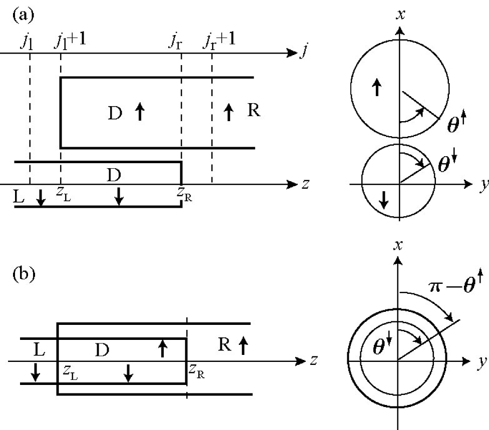
FIG. 1.: Geometrical structures of (a) the side contact and (b) the telescoped coaxial contact. The single wall armchair NTs are denoted by $\downarrow$ and $\uparrow$. The $z$ axis is chosen to be the axis of tube $\downarrow$. The atomic $z$ coordinates in tubes $\downarrow$ and $\uparrow$ are $aj/2$ and $aj/2+\Delta z$, respectively, with integers $j$, the lattice constant $a=0.246$ nm and a small translation $|\Delta z|<a/4$. Tubes $\downarrow$ and $\uparrow$ have the open edges at $z_{\rm R}=aj_{\rm r}/2$ and $z_{\rm L}=\Delta z+a(j_{\rm l}+1)/2$, respectively. The geometrical overlap length is $z_{\rm R}-z_{\rm L}$ while the integer overlap length $N$ is defined as $N=j_{\rm r}-j_{\rm l}+1=2+2(z_{\rm R}-z_{\rm L}+\Delta z)/a$. Without losing generality, $j_{\rm l}=-1,0$.

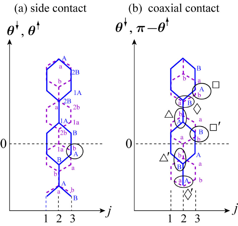
FIG. 2.: Interlayer configuration of (a) the side contact and (b) the coaxial contact for the case where $(n_{\downarrow},n_{\uparrow})=(10,15)$ and $(\Delta\theta,\Delta z)=(0,0)$.

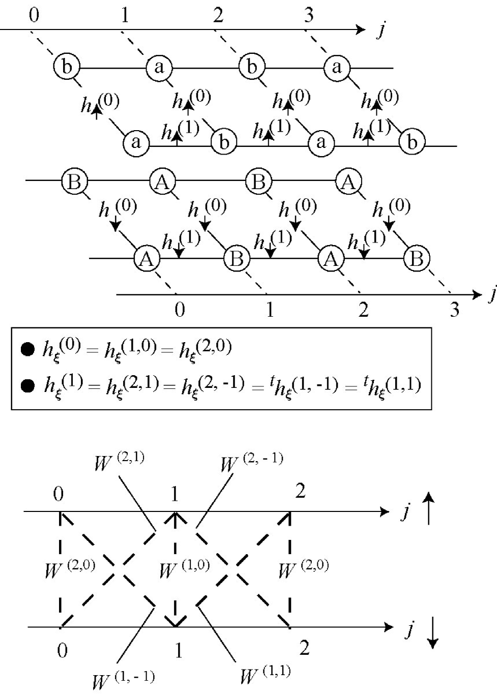
FIG. 3.: Schematic diagram of the tight bindding Hamiltonian. Since $h_{\xi}^{(1,0)}=h_{\xi}^{(2,0)}$ and $h_{\xi}^{(j,1)}=h_{\xi}^{(j,-1)}$, we use the abbreviations $h_{\xi}^{(0)}$ and $h_{\xi}^{(1)}$.

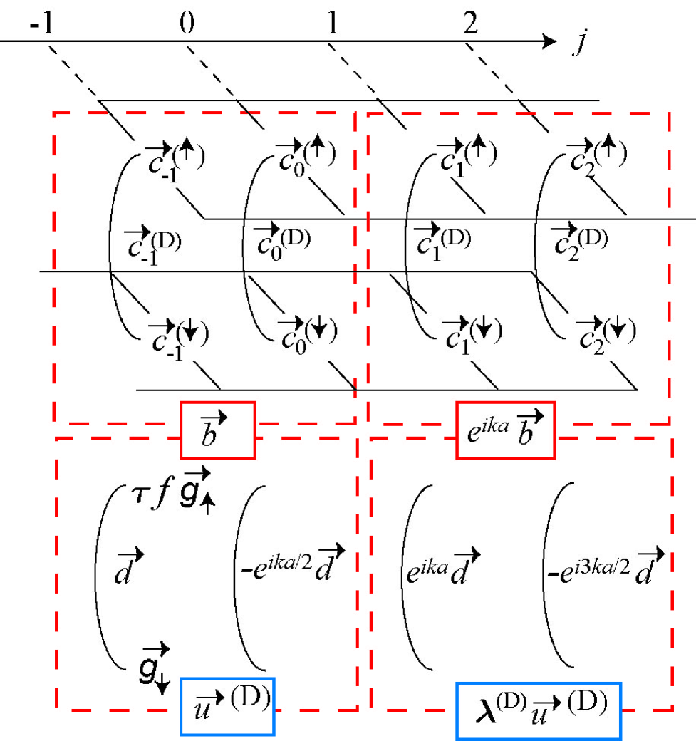
FIG. 4.: Relation between Sec. III A and Sec. III B in notation of the vectors.

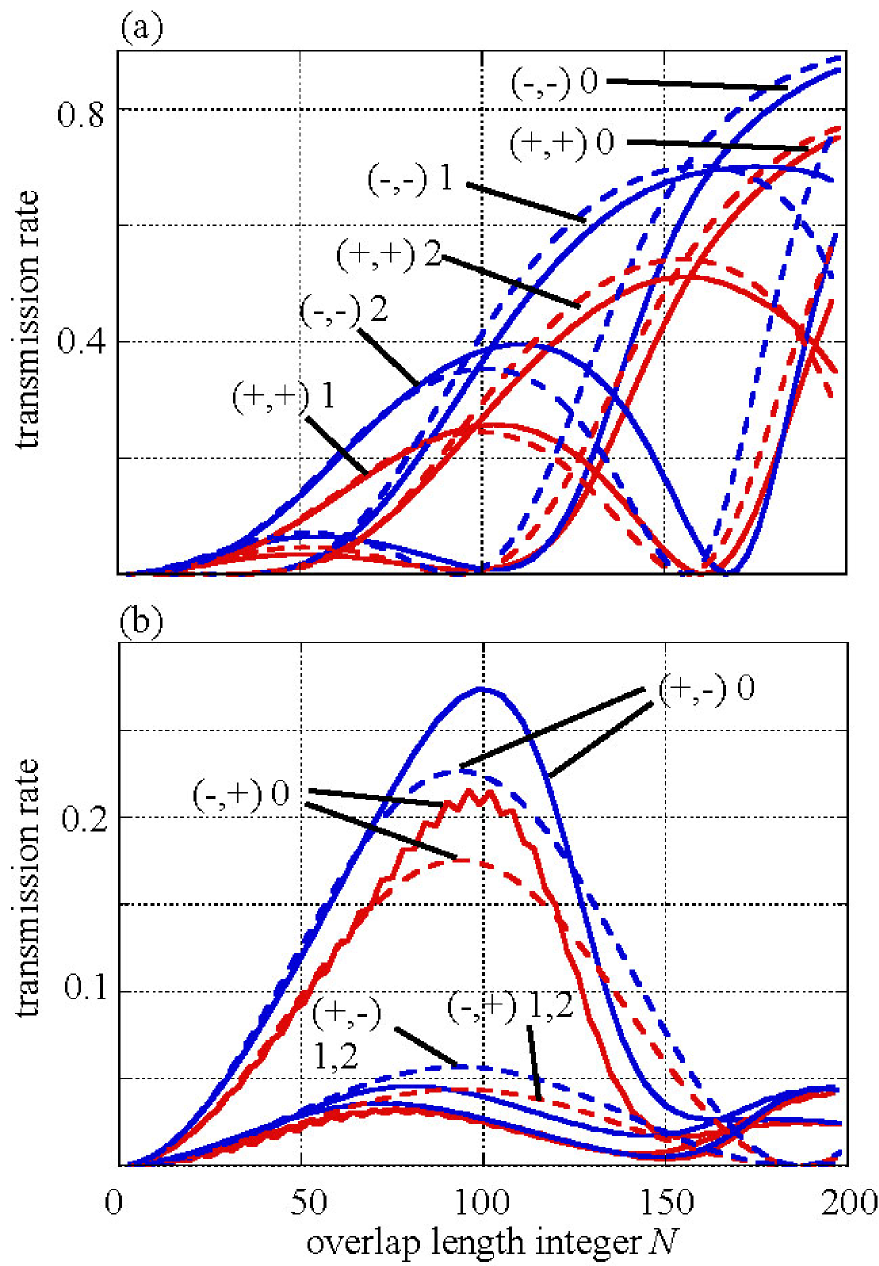
FIG. 5.: (a) Diagonal $T_{\sigma,\sigma}$ and (b) off-diagonal $T_{-\sigma,\sigma}$ transmission rate of the side contact $(n_{\downarrow},n_{\uparrow})=(10,15),j_{\rm l}=-1,\Delta\theta=0,\Delta z=0$ with the energy $E=$ 0.08 eV. The horizontal axis is the integer $N$. The geometrical overlapped length equals $(N-2)a/2$ as is shown by Fig. 1. Solid and dashed lines represent the exact results and the approximate formulas, respectively. By the attached symbols, subscripts of $T_{\sigma^{\prime},\sigma}$ and integers mod($N,3$) are indicated. The labels ’$(\pm,\mp)$ 1’ and ’$(\pm,\mp)$ 2’ are not displayed for the solid lines in (b). Among the four solid lines without the labels, that of $(+,-)$ 1 is slightly larger than the others.

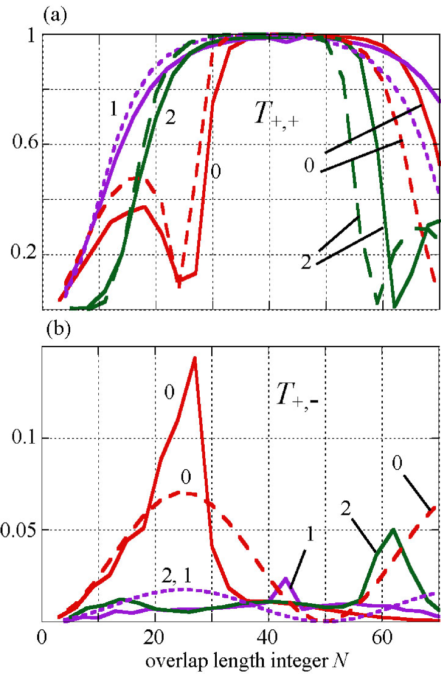
FIG. 6.: Transmission rates (a) $T_{+,+}$ and (b) $T_{+,-}$ of the coaxial contact $(n_{\downarrow},n_{\uparrow})=(10,15),j_{\rm l}=-1,\Delta\theta=0,\Delta z=0$ with the energy $E=$ 0.30 eV. The horizontal axis is the integer $N$. Solid and dashed lines represent the exact results and the approximate formulas, respectively. The attached integers 0, 1 and 2 represent mod($N,3$).

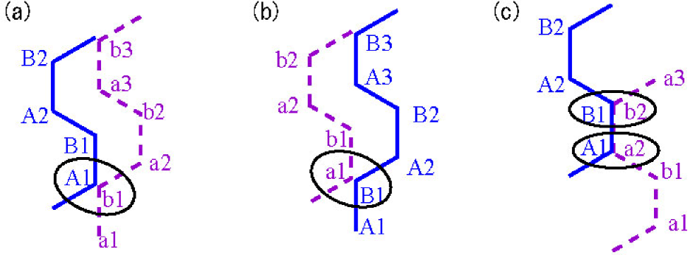
FIG. 7.: Interlayer configuration of bilayer graphenes with (a) Ab , (b) Ba and (c) Aa stacking. Here (A,B) and (a,b) denote sublattices in lower $\downarrow$ and upper $\uparrow$ layers, respectively.

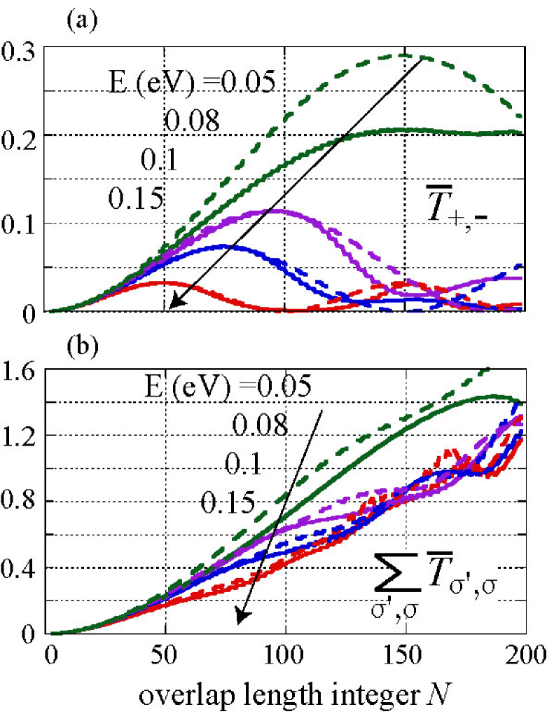
FIG. 8.: (a) $\overline{T}_{+,-}$ and (b) $\sum_{\sigma^{\prime}=\pm}\sum_{\sigma=\pm}\overline{T}_{\sigma^{\prime},\sigma}$ for the energies $E=0.05,0.08,0.1$ and 0.15 eV. Solid and dashed lines represent the exact results and the approximate formulas, respectively. Here $\overline{T}_{\sigma^{\prime},\sigma}(N)$ denotes the smoothed transmission rate of the junction of Fig. 5 defined by $\frac{1}{3}\sum_{j=-1}^{1}T_{\sigma^{\prime},\sigma}(N+j)$.

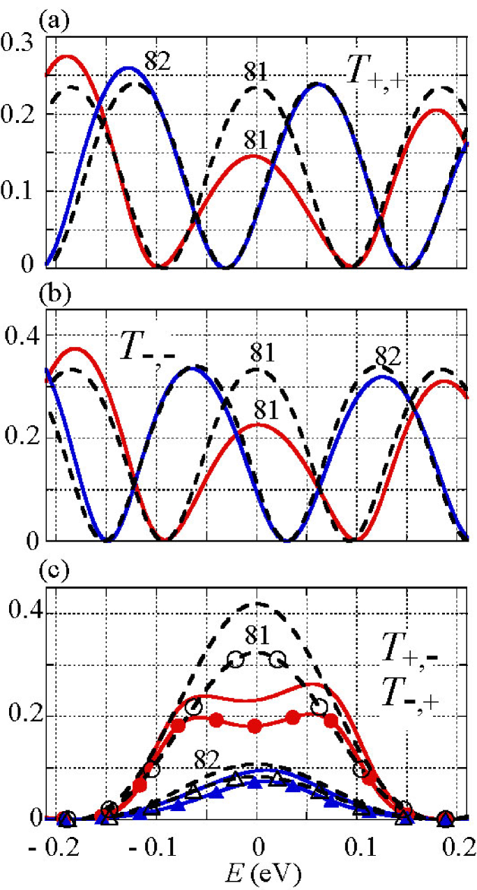
FIG. 9.: Transmission rates (a) $T_{+,+}$ (b) $T_{-,-}$ and (c) $T_{\pm,\mp}$ of the junction of Fig. 5 as a function energy $E$ when $N=81,82$. Solid and dashed lines represent the exact results and the approximate formulas, respectively. In (c), solid lines with closed symbols and dashed lines with open symbols correspond to $T_{-,+}$.

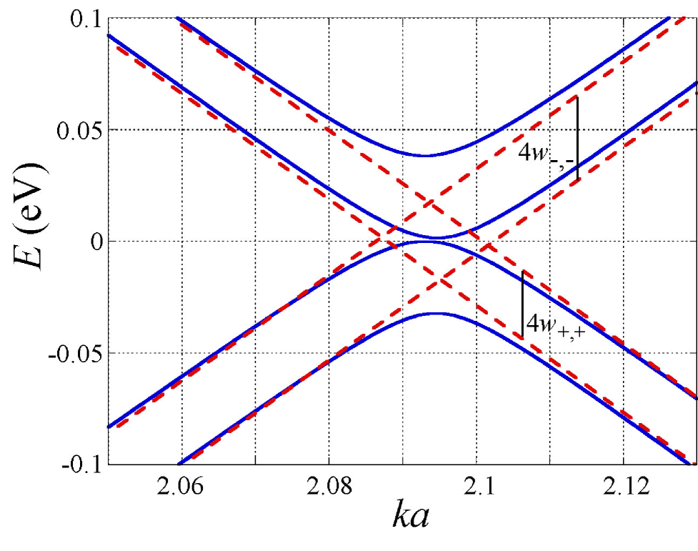
FIG. 10.: The dispersion relation corresponding to region D of the junction of Fig. 5. Solid and dashed lines represent the exact results and the approximate formulas (43), respectively.

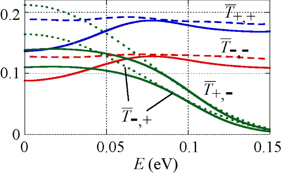
FIG. 11.: Smoothed transmission rates $\frac{1}{3}\sum_{j=-1}^{1}T_{\sigma^{\prime},\sigma}(N+j)$ as a function of the energy $E$ for the junction of Fig. 5 when $N=82$. Solid and dashed lines represent the exact results and the approximate formulas, respectively.

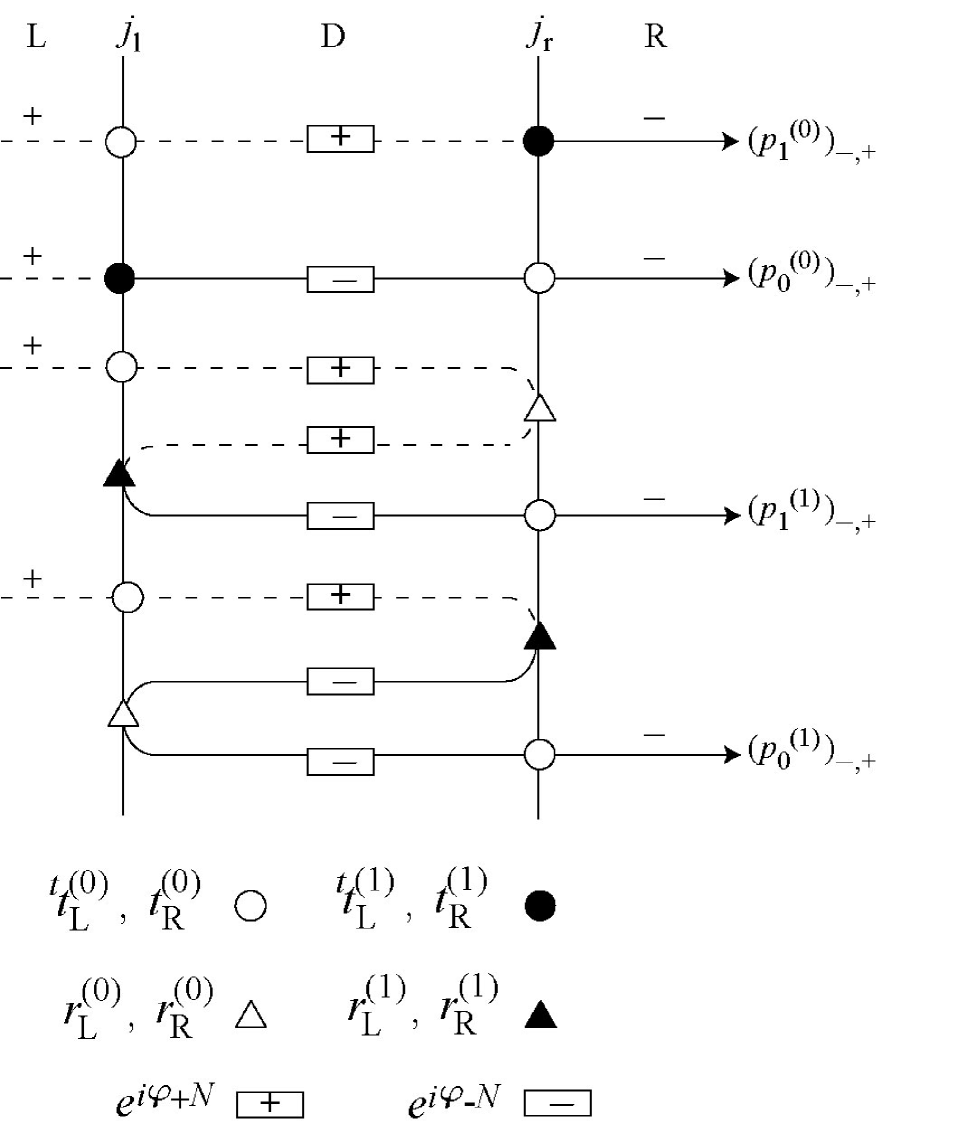
FIG. 12.: Multiple reflection with the notation of Eq. (88) in the case where the symmetric (+) channel is incident from region L.

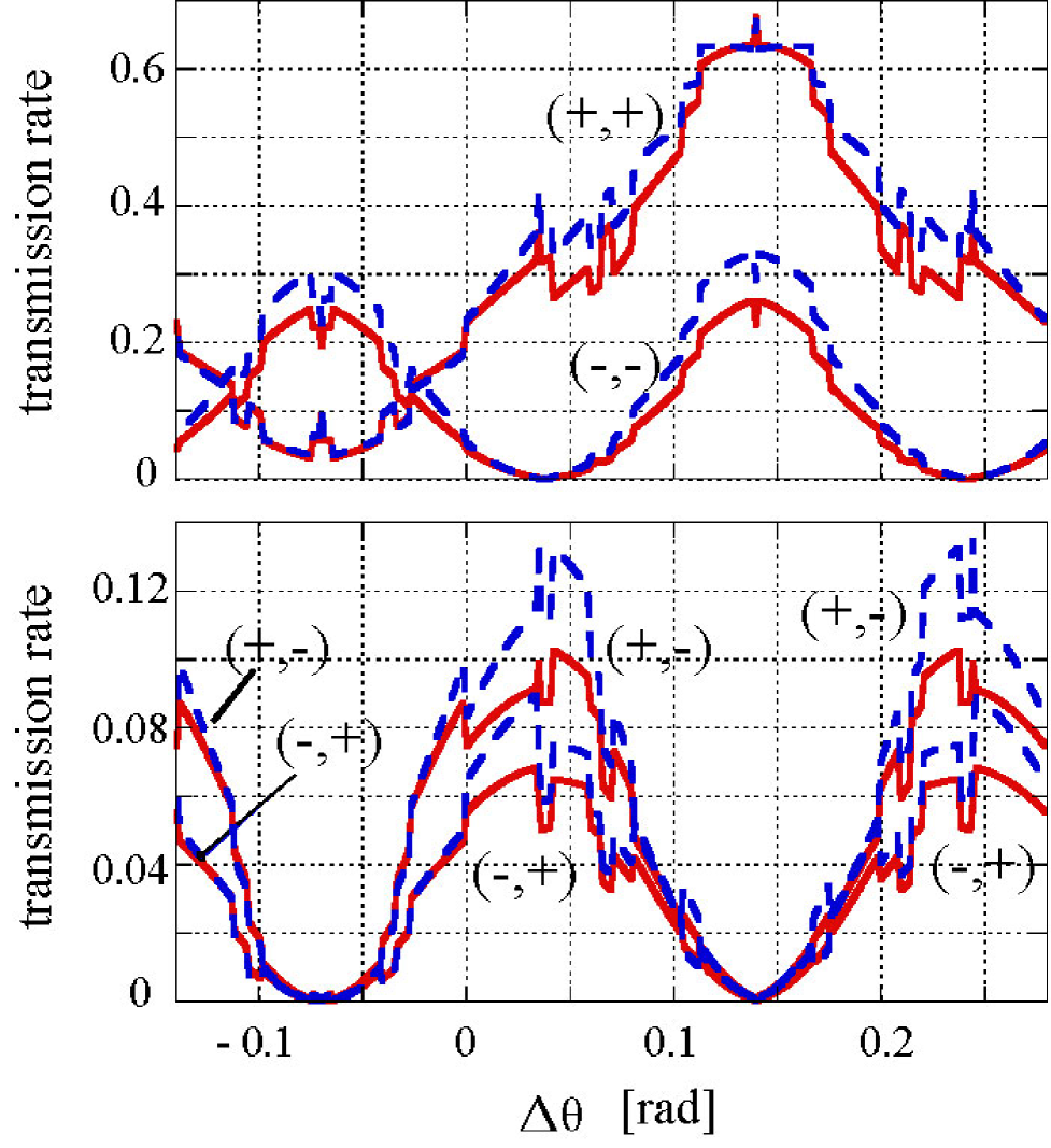
FIG. 13.: Transmission rate $T_{\sigma^{\prime},\sigma}$ as a function of $\Delta\theta$ in the case where $(n_{\downarrow},n_{\uparrow})=(10,15),N=82,\Delta z=0,j_{\rm l}=-1$ and $E=0.05$ eV. Solid and dashed lines represent the exact results and the approximate formulas, respectively. The data are limited to the discrete $\Delta\theta=m\pi/(150n_{\uparrow})$ with intejers $m$.

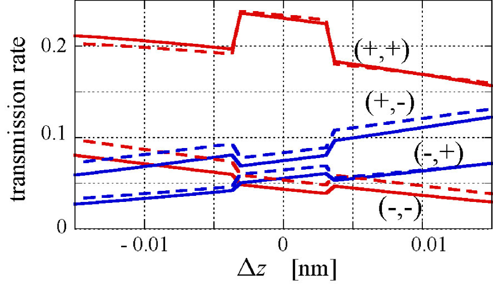
FIG. 14.: The transmission rate $T_{\sigma^{\prime},\sigma}$ as a function of $\Delta z$ in the case where $(n_{\downarrow},n_{\uparrow})=(10,15),N=82,\Delta\theta=0,j_{\rm l}=-1$ and $E=0.05$ eV. Solid and dashed lines represent the exact results and the approximate formulas, respectively. The data are limited to the discrete $\Delta z=ma/400$ with intejers $m$.

REFERENCES

- [1] R. Saito, G. Dresselhaus, and M. S. Dresselhaus, Physical Propertiesof Carbon Nanotubes (Imperial College Press, London,1998).
- [2] J.-C. Charlier, X. Blase, and S. Roche, Rev. Mod. Phys. 79, 677 (2007).
- [3] S. D. Sarma, S. Adam, E. H. Hwang, and E. Rossi, Rev. Mod. Phys. 83, 407 (2011).
- [4] Y.-K. Kwon, S. Saito, and D. Tománek, Phys. Rev. B 58, 13314(R) (1998).;Y.-K. Kwon, and D. Tománek, Phys. Rev. B 58, 16001(R) (1998); Y. Miyamoto, S. Saito, and D. Tománek, ibid. 65, 041402 (2001).
- [5] S. Okada, A. Oshiyama, and S. Saito, Phys. Rev. B 62, 7634 (2000).
- [6] J. Tersoff and R. S. Ruoff, Phys. Rev. Lett. 73, 676 (1994).
- [7] H. M. Abdullah, M. A. Ezzi, and H. Bahlouli, J. of Appl. Phys. 124, 204303 (2018);T.S. Li, Y.C. Huang, S.C. Chang, Y.C. Chuang, and M.F. Lin, Eur. Phys. J. B 64, 73 (2008).
- [8] M. Ochi, M. Koshino, and K. Kuroki, Phys. Rev. B 98, 081102(R) (2018); Y. Cao, V. Fatemi, S. Fang, K. Watanabe, T. Taniguchi, E. Kaxiras, and P. J-Herrero, Nature(London) 556 43 (2018).
- [9] T. Nakanishi, M. Koshino, and T. Ando, Phys. Rev. B 82, 125428 (2010); M. Koshino ibid 88, 115409 (2013).
- [10] J. Cumings and A. Zettl, Science 289, 602 (2000); A. Kis, K. Jensen,S. Aloni, W. Mickelson, and A. Zettl, Phys. Rev. Lett. 97, 025501 (2006); S. Akita and Y. Nakayama, J. J. Appl. Phys. 42, 4830 (2003); M. Nakajima, S. Arai, Y. Saito, F. Arai, and T. Fukuda, ibid. 46, L1035 (2007); W. Zhang, Z. Xi, G. Zhang, C. Li, and D. Guo, Phys. Chem. Lett. 112, 14714 (2008).
- [11] J. Servantie and P. Gaspard, Phys. Rev. B 73, 125428 (2006); Phys. Rev. Lett. 91, 185503 (2003); Q. Zheng and Q. Jiang, Phys. Rev. Lett. 88, 045503 (2002); S. B. Legoas, V. R. Coluci, S. F. Braga, P. Z. Coura, S. O. Dantas, and D. S. Galvao, ibid. 90, 055504 (2003); W. Guo, Y. Guo, H. Gao, Q. Zheng, and W. Zhong. ibid. 91, 125501 (2003); P. Tangney, M. L. Cohen, and S. G. Louie, ibid. 97, 195901 (2006); Q. Zheng, J. Z. Liu, and Q. Jiang, Phys. Rev. B 65, 245409 (2002); J. W. Kang and O. K. Kwon Appl. Sur. Sci. 258, 2014 (2012).
- [12] A. M. Popov, I. V. Lebedeva, A. A. Knizhnik, Y. E. Lozovik, and B. V. Potapkin, Phys. Rev. B 84, 245437 (2011).
- [13] A. Buldum and J. P. Lu, Phys. Rev. Lett., 83, 5050 (1999); M. Seydou, Y. J. Dappe, S. Marsaudon, J.-P. Aimé, X. Bouju, and A.-M. Bonnot, Phys. Rev. B 83, 045410 (2011) ; M. Seydou, S. Marsaudon, J. Buchoux, and J. P. Aimém ibid 80, 245421 (2009).
- [14] Á. Szabados, L. P. Biró, and P. R. Surján, Phys. Rev. B 73, 195404 (2006).
- [15] J. J. Sakurai, Modern quantum mechanics (Addison-Wesley, Tokyo, 1994).
- [16] M. Koshino and T. Ando, Phys. Rev. B 76, 085425 (2007); J. Nilsson, A. H. C. Neto, F. Guinea and N. M. R. Peres, ibid 78, 045405 (2008); J. Ruseckas, G. Juzeliunas and I. V. Zozoulenko, ibid B 83, 035403 (2011); F. Zhang, Bhagawan Sahu, H. Min and A. H. MacDonald, ibid 82, 035409 (2010) B. Partoens and F. M. Peeters Phys. Rev. B 74, 075404 (2006); 75, 193402 (2007).
- [17] J-L. Zhu, F-F. Xu and Y-F. Jia, Phys. Rev. B 74, 155430 (2006); M. Terrones, F. Banhart, N. Grobert, J.-C. Charlier, H. Terrones and P. M. Ajayan, Phys. Rev. Lett. 89, 075505 (2002); F. Y. Meng,S. Q. Shi, D. S. Xu and R. Yang, Phys. Rev. B 70, 125418 (2004); A. V. Krasheninnikov, K. Nordlund, J. Keinonen and F. Banhart, ibid 66, 245403 (2002); S. Dag, R. T. Senger, and S. Ciraci, ibid 70, 205407 (2004).
- [18] D, Valencia, J-Q, Lu, J. Wu, F. Liu, F. Zhai, and Y-J. Jiang ,AIP Advances 3, 102125 (2013); J. Nilsson, A. H. Castro Neto, F. Guinea and N. M. R. Peres, Phys. Rev. B 76, 165416 (2007).
- [19] J. Cumings and A. Zettl, Phys. Rev. Lett. 93, 086801 (2004); S. Akita and Y. Nakayama, J. J. Appl. Phys. 43, 3796 (2004).
- [20] D. Yin, W. Liu , X. Li, L. Geng, X. Wang and P. Huai, Appl. Phys. Lett. 103, 173519 (2013); J. W. Gonzalez, H. Santos, M. Pacheco, L. Chico and L. Brey, Phys. Rev. B 81, 195406 (2010); J. Zheng, P. Guo, Z. Ren, Z. Jiang, J. Bai, and Z. Zhang, Appl. Phys. Lett. 101, 083101 (2012); X-G. Li, I-H. Chu, X.-G. Zhang and H-P. Cheng, Phys. Rev. B 91, 195442 (2015); H. M. Abdullah, B. V. Duppen, M. Zarenia, H. Bahlouli, and F. M. Peeters, J. Phys. Condens. Matter 29, 425303 (2017); I. V. Lebedeva , A. M. Popov , A. A. Knizhnik, Y. E. Lozovik, N. A. Poklonski, A. I. Siahlo, S. A. Vyrko, S. V. Ratkevich, Comp. Mat. Sci. 109 240 (2015) .
- [21] B. G. Cook, W. R. French, and K. Varga, Appl. Phys. Lett. 101, 153501 (2012).
- [22] Q. Yan, G. Zhou, S. Hao, J. Wu, and W. Duan, Appl. Phys. Lett. 88, 173107 (2006); A. Hansson and S. Stafstrom, Phys. Rev. B, 67, 075406 (2003); I. M. Grace, S. W. Bailey, and C. J. Lambert, Phys. Rev. B, 70, 153405 (2004);Y.-J. Kang, K. J. Chang, and Y.-H. Kim, Phys. Rev. B 76, 205441 (2007).
- [23] R. Tamura, Phys. Rev. B 82, 035415 (2010); 86, 205416 (2012).
- [24] D.-H. Kim and K. J. Chang, Phys. Rev. B, 66, 155402 (2002).
- [25] R. Tamura, Y. Sawai, and J. Haruyama, Phys. Rev. B 72, 045413 (2005).
- [26] S. Uryu and T. Ando, Phys. Rev. B 76, 155434 (2007);72, 245403 (2005).
- [27] S. Tripathy and T. K. Bhattacharyya, Physica E 83, 314 (2016); Q. Liu, G. Luo, R. Qin, H. Li, X. Yan, C. Xu, L. Lai, J. Zhou, S. Hou, E. Wang, Z. Gao and J. Lu, Phys. Rev. B 83, 155442 (2011); A. Buldum and J. P. Lu,Phys. Rev. B 63, 161403(R) (2001).
- [28] F. Xu, A. Sadrzadeh, Zhiping Xu and B. I. Yakobson, J. Appl. Phys. 114, 063714 (2013).
- [29] C. Buia, A. Buldum, and J. P. Lu, Phys. Rev. B, 67, 113409 (2003).
- [30] M. A. Tunney and N. R. Cooper, Phys. Rev. B 74, 075406 (2006).
- [31] S. Datta, Electronic Transport in Mesoscopic Systems (Cambridge University Press, Cambridge 1995).
- [32] T. Nakanishi and T. Ando, J. Phys. Soc. Jpn 70, 1647 (2001); Y-G. Yoon, M. S. C. Mazzoni, H. J. Choi, J. Ihm, and S. G. Louie, Phys. Rev. Lett 86 688 (2001);A. A. Maarouf and E. J. Mele, Phys. Rev. B 83 , 045402 (2011); B. G. Cook, P. Dignard, and K. Varga, Phys. Rev. B 83, 205105 (2011).
- [33] Ph. Lambin, V. Meunier and A. Rubio, Phys. Rev. B 62 5129 (2000);J. -C. Charlier, J. -P. Michenaud and Ph. Lambin, ibid 46 4540 (1992).
- [34] Single valued eV) of the present work and multivalued 0.36 eV, 0.16 eV) of Ref. [25] show that and , respectively, for the coaxial contact under the conditions mod( and . This difference is explained with the term ’three fold cancellation’ in Ref. [25].