Universal Deep Beamformer for Variable Rate Ultrasound Imaging

Abstract

Ultrasound (US) imaging is based on the time-reversal principle, in which individual channel RF measurements are back-propagated and accumulated to form an image after applying specific delays. While this time reversal is usually implemented as a delay-and-sum (DAS) beamformer, the image quality quickly degrades as the number of measurement channels decreases. To address this problem, various types of adaptive beamforming techniques have been proposed using predefined models of the signals. Unfortunately, the performance of these adaptive beamforming approaches degrade when the underlying model is not sufficiently accurate. Here, we demonstrate for the first time that a single universal deep beamformer trained using a purely data-driven way can generate significantly improved images over widely varying aperture and channel subsampling patterns. In particular, we design an end-to-end deep learning framework that can directly process sub-sampled RF data acquired at different subsampling rate and detector configuration to generate high quality ultrasound images using a single beamformer. Experimental results using B-mode focused ultrasound confirm the efficacy of the proposed methods.

I Introduction

Excellent temporal resolution with reasonable image quality makes ultrasound (US) modality a first choice for variety of clinical applications . Moreover, due to its minimal invasiveness from non-ionizing radiations, US is an indispensable tool for some clinical applications such as cardiac, fetal imaging, etc.

The basic imaging principle of US imaging is based on the time-reversal [1, 2], which is based on a mathematical observation that the wave operator is self-adjoint. In other words, the wave operator is invariant under time transformation $t\rightarrow-t$, and the position of the sources and receivers can be swapped. Therefore, it is possible to reverse a wave from the measurement positions and different control times to the source locations and the initial time. Practically, this is done by back-propagating the measured data, after the delay transformation $t\rightarrow t_{\max}-t$, through adjoint wave and adding all the contributions.

For example, in focused B-mode US imaging, the return echoes from individual scan line are recorded by the receiver channels, after which delay-and-sum (DAS) beamformer applies the time-reversal delay to the channel measurement and additively combines them for each time point to form images at each scan line.

Despite the simplicity, large number of receiver elements are often necessary in time reversal imaging to improve the image quality by reducing the side lobes. Similarly, high-speed analog-to-digital converters (ADC) should be used. This is because the mathematical theory of time reversal is derived assuming that the distance between consecutive receivers is taken to be less than half of the wavelength and the temporal scanning is done at a fine rate so that the relative difference between consecutive scanning times is very small [1, 2]. Therefore, with the limited number of receive channels and ADC resolution, DAS beamformer suffers from reduced image resolution and contrast.

To address this problem, various adaptive beamforming techniques have been developed over the several decades [3, 4, 5, 6, 7, 8, 9, 10, 11]. The main idea of adaptive beamforming is to change the receive aperture weights based on the received data statistics to improve the resolution and enhance the contrast. For example, one of the most extensively studied adaptive beamforming technique is the Capon beamforming, also known as the minimum variance (MV) beamforming [4, 5, 6]. The aperture weight of Capon beamfomer is derived by minimizing the side lobe while maintaining the gain at the look-ahead direction. Unfortunately, Capon beamforming is computational heavy for practical use due to the calculation of the covariance matrix and its inverse [7]. Moreover, the performance of Capon beamformer is dependent upon the accuracy of the covariance matrix estimate. To reduce the complexity, many improved version of MV beamformers have been proposed [6, 7, 8, 9]. Some of the notable examples includes the beamspace adaptive beamformer [8], multi-beam Capon based on multibeam covariance matrices[10]. To improve the robustness of Capon beamformer, parametric form of the covariance matrix calculation with iterative update was also proposed rather than calculating the empirical covariance matrix [11].

However, Capon beamformer and its variants are usually designed for uniform array, so it is difficult to use for the subsampled sparse array that is often used to reduce the power consumption and data rate [12, 13]. To address this, compressed sensing (CS) approaches have been recently studied. In [12], Colas et al. proposed a point-spread-functions based sensing matrix for CS reconstruction. However, the accurate measurement of the spatially varying point spread function is difficult, which limits the resolution for in vivo experiments [12]. In [14, 15, 16], compressive beamforming methods were proposed. But these approaches usually require changes of ADC part of hardwares.

Recently, inspired by the tremendous success of deep learning, many researchers have investigated deep learning approaches for various inverse problems [17, 18, 19, 20, 21, 22, 23, 24, 25, 26, 27, 28]. In US literature, the works in [29, 30] were among the first to apply deep learning approaches to US image reconstruction. In particular, Allman et al [29] proposed a machine learning method to identify and remove reflection artifacts in photo-acoustic channel data. Luchies and Byram [30] proposed a frequency domain deep learning method for suppressing off-axis scattering in ultrasound channel data. In [31], a deep neural network is designed to estimate the attenuation characteristics of sound in human body. In [32, 33], ultrasound image denoising method is proposed for the B-mode and single angle plane wave imaging, respectively. Rather than using deep neural network as a post processing method, the authors in [13, 34, 35, 36] use deep neural networks for the reconstruction of high-quality US images from limited number of received RF data. For example, the work in [34] uses deep neural network for coherent compound imaging from small number of plane wave illumination. In focused B-mode ultrasound imaging, [13] employs the deep neural network to interpolate the missing RF-channel data with multiline aquisition for accelerated scanning. In [35, 36], the authors employ deep neural networks for the correction of blocking artifacts in multiline acquisition and transmission scheme.

While these recent deep neural network approaches provide impressive reconstruction performance, the current design is not universal in the sense that the designed neural network cannot completely replace a DAS beamformer, since they are designed and trained for specific acquisition scenario. Similar limitation exists in the classical MV beamformer, since the covariance matrix is determined by the specific detector geometry, which is difficult to adapt, for example, to dynamically varying sparse array [37].

Therefore, one of the most important contributions of this paper is to demonstrate that a single beamformer can generate high quality images robustly for various detector channel configurations and subsampling rates. The main innovation of our universal deep beamformer comes from one of the most exciting properties of deep neural network - exponentially increasing expressiveness [38, 39, 40]. For example, Arora et al [40] showed that for every natural number $k$ there exists a ReLU network with $k^{2}$ hidden layers and total size of $k^{2}$, which can be represented by $\frac{1}{2}k^{k+1}-1$ neurons with at most $k$-hidden layers. All these results agree that the expressive power of deep neural networks increases exponentially with the network depth. Thanks to the exponential large expressiveness with respect to depth, our novel deep neural network beamformer can learn the mapping to images from various sub-sampled RF measurements, and exhibits superior image quality for all sub-sampling rate. Another amazing feature of the proposed network is that even though the network is trained to learn the mapping from the sub-sampled channel data to the B-mode images from full rate DAS images, the trained neural network can utilize the fully sampled RF data furthermore to improve the image contrast even for the full rate cases.

This paper is organized as follows. In Section II, a brief survey of the existing adaptive beamforming methods are provided, which is followed by the detailed explanation of the proposed universal beamformer. Section III then describes the data set and experimental setup. Experimental results are provided in Section IV, which is followed by Discussion and Conclusions in Section V and Section VI.

II Theory

II-A Adaptive Beamforming

The standard non-gain compensated delay-and-sum (DAS) beamformer for the $l$-th scanline at the depth sample $n$ can be expressed as

$${z}_{l}[n]=\frac{1}{J}\sum_{j=0}^{J-1}x_{l,j}[n-\tau_{j}[n]]=\frac{1}{J}\mathbf{1}^{\top}\mathbf{y}_{l}[n],\quad l=0,\cdots,L-1$$ (1)

where ^⊤ denotes the transpose, $x_{l,j}[n]$ is the RF echo signal measured by the $j$-th active receiver element from the transmit event (TE) for the $l$-th scan line, and $J$ denotes the number of active receivers, $\tau_{j}[n]$ is the dynamic focusing delay for the $j$-th active receiver elements to obtain the $l$-th scan line. Furthermore, ${\mathbf{y}}_{l}[n]$ refers to the scan line dependent time reversed RF data defined by

$$\mathbf{y}_{l}[n]=\begin{bmatrix}y_{l,0}[n]&y_{l,1}[n]&\cdots&y_{l,J-1}[n]]\end{bmatrix}^{\top}$$ (2)

with $y_{l,j}[n]:=x_{l,j}\left[n-\tau_{j}[n]\right]$, and $\mathbf{1}$ denotes a length $J$ column-vector of ones.

This averaging of the time-delayed element-outputs extracts the (spatially) low-frequency content that corresponds to the energy within one scan resolution cell (or main lobe). Reduced side lobe leakage at the expense of a wider resolution cell can be achieved by replacing the uniform weights by tapered weights $w_{l,j}[n]$:

$$z_{l}[n]=\sum_{j=0}^{J-1}w_{l,j}[n]y_{l,j}[n]={\mathbf{w}}_{l}[n]^{\top}{\mathbf{y}}_{l}[n]$$ (3)

where $\mathbf{w}_{l}[n]=\begin{bmatrix}w_{l,0}[n]&w_{l,1}[n]&\cdots&w_{l,J}[n]\end{bmatrix}^{\top}.$ In adaptive beamforming the objective is to find the $\mathbf{w}_{l}$ that minimizes the variance of ${z}_{l}$, subject to the constraint that the gain in the desired beam direction equals unity. The minimum variance (MV) estimation task can be formulated as [4, 5, 6]

$$\underset{\mathbf{w}_{l}[n]}{\text{minimize}} E[|z_{l}[n]|^{2}]=\min_{\mathbf{w}[n]}\mathbf{w}_{l}[n]^{\top}\mathbf{R}_{l}[n]\mathbf{w}_{l}[n]$$

subject to $$\mathbf{w}_{l}[n]^{H}{\mathbf{a}}=1,$$

where $E[\cdot]$ is the expectation operator, and $\mathbf{a}$ is a steering vector, which is composed of ones when the received signal is already temporally aligned, and $\mathbf{R}[n]$ is a spatial covariance matrix expressed as

$$\mathbf{R}_{l}[n]=E\left[\mathbf{y}_{l}[n]^{\top}\mathbf{y}_{l}[n]\right],$$ (4)

Then, ${\mathbf{w}}_{l}[n]$ can be obtained by Lagrange multiplier method [41] and expressed as

$$\mathbf{w}_{l}[n]=\frac{\mathbf{R}_{l}[n]^{-1}\mathbf{a}}{\mathbf{a}^{H}\mathbf{R}_{l}[n]^{-1}\mathbf{a}}.$$ (5)

In practice, $\mathbf{R}_{l}[n]$ must be estimated with a limited amount of data. A widely used method for the estimation of $\mathbf{R}_{l}[n]$ is spatial smoothing (or subaperture averaging) [42], in which the sample covariance matrix is calcualted by averaging covariance matrices of $K$ consecutive channels in the $J$ receiving channels as follows:

$$\mathbf{\tilde{R}}_{l}[n]=\frac{1}{J-K+1}{\mathbf{Y}_{l}}[n]{\mathbf{Y}_{l}}^{\top}[n],$$ (6)

where

$${\mathbf{Y}_{l}}[n]=\begin{bmatrix}y_{l,0}[n]&\dots&y_{l,J-K}[n]\\ \vdots&&\vdots\\ y_{l,K-1}[n]&\dots&y_{l,J-1}[n]\end{bmatrix},$$ (7)

which is invertible if $K\leq J/2$. To further improve the invertibility of the sample covariance matrix, another method usually called diagonal loading is often used by adding additional diagonal terms [42].

One of the problems with the MV beamforming technique employed in a medical ultrasound imaging system is that the speckle characteristics tend to be different from those of conventional DAS beamformed images. MV beamformed images tend to look slightly different from conventional DAS B-mode images in that the speckle region appears to have many small black dots interspersed (see [42, Fig. 6]). To overcome this problem, a temporal averaging method [43] that averages $\mathbf{\tilde{R}}$ along the depth direction is used, which is expressed as

$$\mathbf{\tilde{R}}_{l}[n]=\frac{1}{2L+1}\frac{1}{J-K+1}\sum_{l=-L}^{L}{\mathbf{Y}_{l}}[n+l]{\mathbf{Y}_{l}}^{\top}[n+l],$$ (8)

Another method to estimate the covariance matrix in MV is so-called multibeam approach [10]. In this method, the weight vector is estimated using empirical covariance matrices that are formed to use phase-based (narrowband) steering vectors to extract the adaptive array weights from it.

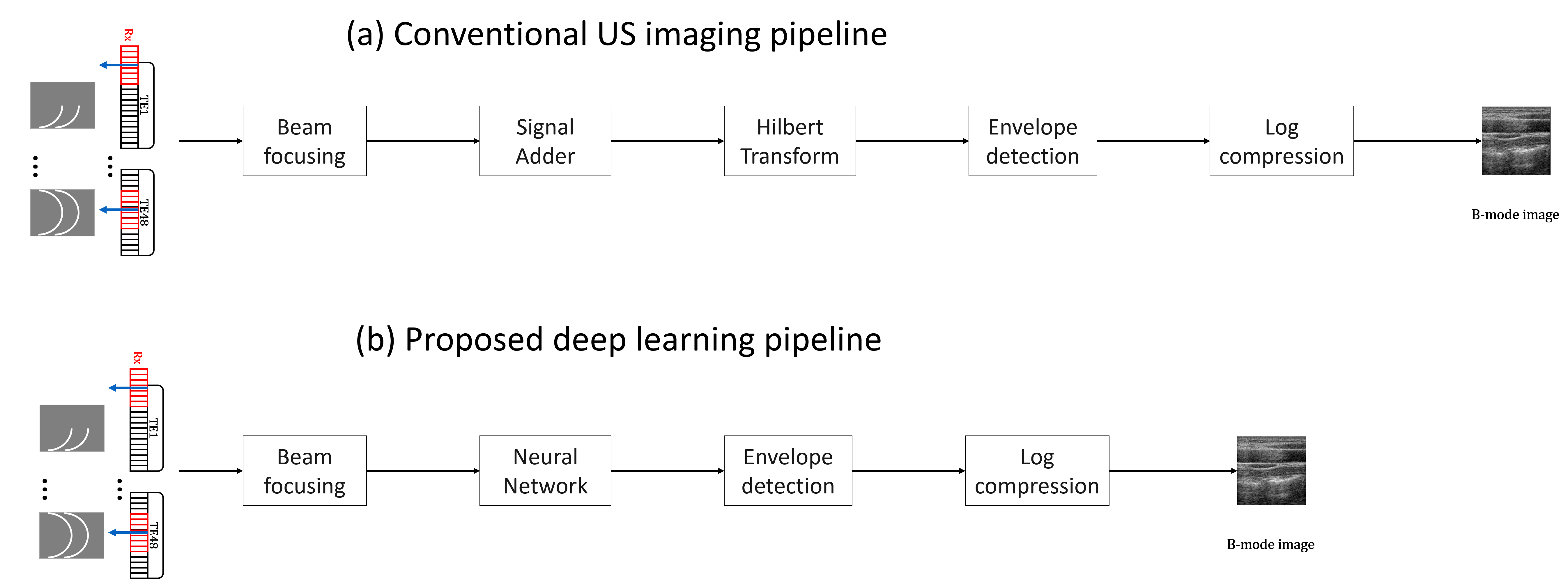
Figure 1: Ultrasound imaging pipeline. (a) standard focused B-mode pipeline, and (b) the proposed neural network based reconstruction pipeline.

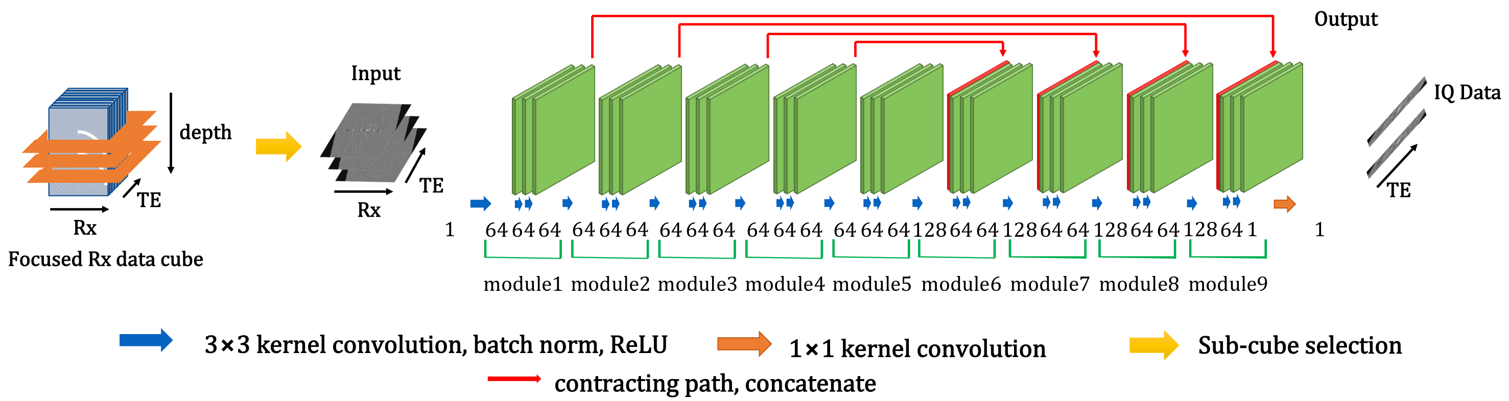
Figure 2: Proposed CNN based Ultrasound imaging system block diagram.

II-B Proposed algorithm

II-B1 Image reconstruction pipeline

Fig. 1(a) illustrates the conventional US image reconstruction piplelne. Here, the reflected sound waves in the medium are detected by the transducer elements. Each measured signal is time reversed based on the traveled distance to perform beam-focusing. The focused signals are later added. In this paper, the adaptive beamformer can be used for providing adaptive summation of the time-reversed echos. This is then followed by the Hilbert transform to detector the envelope of the beam. In particular, the envelop is determined by calculating the absolute value of the inphase and quadrature pahse signals generated from the Hilbert transform. Finally, the log compression is applied to generate the B-mode images.

On the other hand, our goal is to replace the the signal adder and Hilbert transformation step by a convolutional neural network (CNN) as shown in Fig. 1(b). Time reversal part is still based on the physical delay calculation, since this is the main idea of the time reversal algorithms. Envelop detection and log compression are just a simple point-wise operation, so the neural network is not necessary. Therefore, our goal is to basically replace the core beamformer and reconstruction engine with a data-driven way CNN.

II-B2 Universal Deep Beamformer

Recall that the basic idea of adaptive beamformer is to estimate the array weight ${\mathbf{w}}_{l}[n]$ from the data to estimate $z_{l}[n]$, which changes with respect to the scan line index $l$ and the depth $n$. In the conventional adaptive beamformer, this estimation is usually done based on the linear weight model calculated from the empirical covariance. However, this linear model is usually based on restricted assumption, such as zero mean, Gaussian noise, etc, which may limit the fundamental performance of the adaptive beamformer. Moreover, nonlinear beamforming methods have been recently proposed to overcome the limitation of linear model[44, 45, 46, 47]. Another important step after the beamforming is the Hilbert transform to obtain analytic representation. More specifically, Hilbert transform gives the analytic representation of a signal u(t):

$$z_{l}^{a}[n]=z_{l}[n]+\iota H(z_{l})[n]$$ (9)

where $\iota=\sqrt{-1}$, and $H$ denotes the Hibert transform. $z_{l}^{a}[n]$ is often referred to as the inphase (I) and quadrature (Q) representation. To implement Hilbert transform, discrete convolution operation is usually performed for each scan line along the depth direction.

One of the main key ideas of the proposed method is a direct estimation of the beamfored and Hilbert transformed signal $z_{l}^{a}[n]$ directly from the time-reverse signal ${\mathbf{y}}_{l}[n]$ using convolutional neural network. To exploit the redundancies along the scan line direction, rather than estimating the beamformed signal for each scan line, we are interested in estimating the beamformed and Hilbert transformed signal at whole scan line, i.e.

$${\mathbf{z}}^{a}[n]=\begin{bmatrix}z_{0}^{a}[n]&\cdots&z_{L-1}^{a}[n]\end{bmatrix}^{\top}$$

Furthermore, to deal with the potential blurring along the depth, we are interested in exploiting the time reversed signal at three depth coordinates, i.e.

$${\mathbf{Y}}[n]=\begin{bmatrix}{\mathbf{y}}_{0}[n-1]&{\mathbf{y}}_{1}[n-1]&\cdots&{\mathbf{y}}_{L-1}[n-1]\\ {\mathbf{y}}_{0}[n]&{\mathbf{y}}_{1}[n]&\cdots&{\mathbf{y}}_{L-1}[n]\\ {\mathbf{y}}_{0}[n+1]&{\mathbf{y}}_{1}[n+1]&\cdots&{\mathbf{y}}_{L-1}[n+1]\end{bmatrix}$$ (10)

Then, our goal is to estimate the nonlinear function $f({\mathbf{W}},{\mathbf{Y}}[n])$ such that

$${\mathbf{z}}^{a}[n]=f({\boldsymbol{\Theta}},{\mathbf{Y}}[n])$$

where ${\boldsymbol{\Theta}}$ denotes the trainable CNN parameters. To generate the complex output, our neural network generates the two channel output that corresponds to the real and image parts. Then, our CNN called deep beamformer (DeepBP) is trained as follows:

$$\min_{\Theta}\sum_{i=1}^{T}\sum_{n}\|{\mathbf{z}}^{a(i)}[n]-f({\boldsymbol{\Theta}},{\mathbf{Y}}^{(i)}[n])\|^{2}$$ (11)

where ${\mathbf{z}}^{a(i)}[n]$ denotes the ground-truth I-Q channel data at the depth $n$ from the $i$-th training data, and ${\mathbf{Y}}^{(i)}[n]$ represented the corresponding (sub-sampled) time-delayed input data formed by (10).

Note that our current training scheme is depth-independent so that the same CNN can be used across all depth. Furthermore, as for the target data for the training, we use the standard DAS beamformed data from full detector samples. Since the target data is obtained from various depth across multiple scan lines, our neural network is expected to learn the best parameters on averages. Interestingly, this average behavior turns out to improve the overall image quality even without any subsampling thanks to the synergistic learning from many training data, as will be shown later in experiments.

Fig. 2 illustrates the schematic diagram of our deep beamformer. In particular, we trained our model with the input/output pairs of a three depth of Rx-TE-Depth data cube as an input and the I-Q data on a single Rx-TE plane as a target.

III Method

III-A Data set

For experimental verification, multiple RF data were acquired with the E-CUBE 12R US system (Alpinion Co., Korea). For data acquisition, we used a linear array transducer (L3-12H) with a center frequency of $8.48$ MHz. The configuration of the probe is given in Table I.

TABLE I: Probe Configuration

Parameter	Linear Probe
Probe Model No.	L3-12H
Carrier wave frequency	8.48 MHz
Sampling frequency	40 MHz
No. of probe elements	192
No. of Tx elements	128
No. of TE events	96
No. of Rx elements	64
Elements pitch	0.2 mm
Elements width	0.14 mm
Elevating length	4.5 mm

Using a linear probe, we acquired RF data from the carotid area from $10$ volunteers. The in-vivo data consists of $40$ temporal frames per subject, providing $400$ sets of Depth-Rx-TE data cube. The dimension of each Rx-TE plane was $64\times 96$. A set of $30,000$ Rx-TE planes was randomly selected from the $4$ subjects datasets, and data cubes (Rx-TE-depth) are then divided into $25,000$ datasets for training and $5000$ datasets for validation. The remaining dataset of $360$ frames was used as a test dataset.

In addition, we acquired $188$ frames of RF data from the ATS-539 multipurpose tissue mimicking phantom. This dataset was only used for test purposes and no additional training of CNN was performed on it. The phantom dataset was used to verify the generalization power of the proposed algorithm.

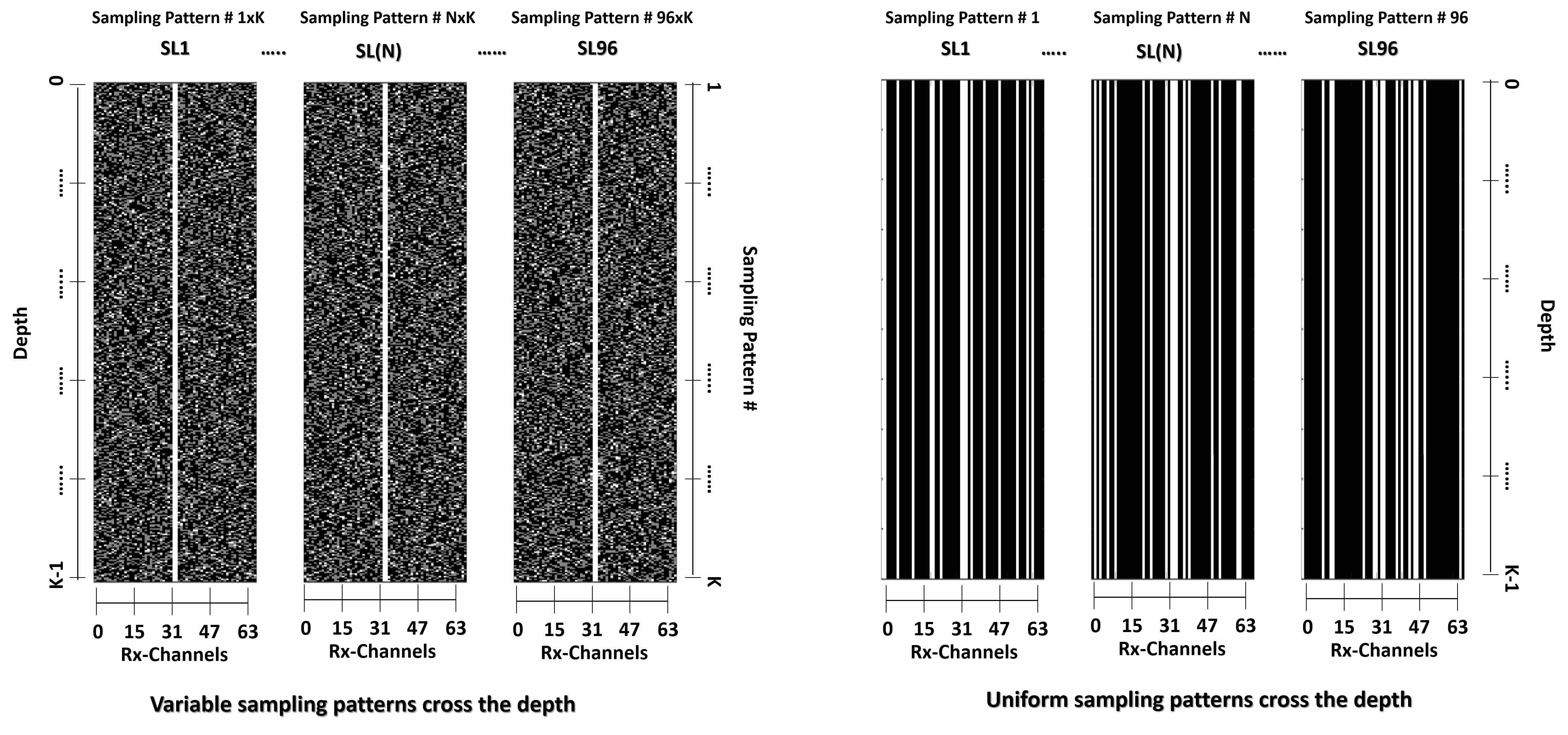
Figure 3: (left) sampling scheme # 1: variable sampling cross depth axis. (right) sampling scheme # 2: uniform sampling cross depth axis.

III-B RF Sub-sampling Scheme

For our experiments, we generated six sets of sub-sampled RF data at different down-sampling rates. In particular, we use several subsampling cases using $64$, $32$, $24$, $16$, $8$ and $4$ Rx-channels, and two subsampling schemes were used: variable down-sampling pattern cross the depth, fixed down-sampling pattern cross the depth (see Figs. 3).

Since the active receivers at the center of the scan-line get RF data from direct reflection, the two channels that are in the center of active transmitting channels were always included to improve the performance, and remaining channels were randomly selected from the total $64$ active receiving channels. In variable sampling scheme, different sampling pattern (mask) is used for each depth plane whereas, in fixed sampling, we used same sampling pattern (mask) for all depth planes. The network was trained for variable sampling scheme only and both sampling schemes were used in test phase.

III-C Network Architecture

For all sub-sampling schemes samples, a multi-channel CNN was applied to $3\times 64\times 96$ data-cube in the depth-Rx-TE sub-space to generate a $2\times 3\times 96$ I and Q data in the depth-TE plane. The target IQ data is obtained from two output channels each representing real and imaginary parts.

The proposed CNN is composed of convolution layers, batch normalization layers, ReLU layers and a contracting path with concatenation as shown in Figs. 2(b). Specifically, the network consists of $29$ convolution layers composed of a batch normalization and ReLU except for the last convolution layer. The first $28$ convolution layers use $3\times 3$ convolutional filters (i.e. the 2-D filter has a dimension of $3\times 3$), and the last convolution layer uses a $1\times 1$ filter and contract the $3\times 64\times 96$ data-cube from depth-Rx-TE sub-space to $2\times 3\times 96$ IQ-depth-TE plane.

The network was implemented with MatConvNet [48] in the MATLAB 2015b environment. Specifically, for network training, the parameters were estimated by minimizing the $l_{2}$ norm loss function. The network was trained using a stochastic gradient descent with a regularization parameter of $10^{-4}$. The learning rate started from $10^{-4}$ and gradually decreased to $10^{-7}$. The weights were initialized using Gaussian random distribution with the Xavier method [49]. The number of epochs was $200$ for all down-sampling rates.

III-D Performance Metrics

To quantitatively show the advantages of the proposed deep learning method, we used the contrast-to-noise ratio (CNR) [50], generalized CNR (GCNR) [51], peak-signal-to-noise ratio (PSNR), structure similarity (SSIM) [52] and the reconstruction time.

The CNR is measured for the background ($B$) and anechoic structure ($aS$) in the image, and is quantified as

$${\hbox{CNR}}(B,aS)=\frac{|\mu_{B}-\mu_{aS}|}{\sqrt{\sigma^{2}_{B}+\sigma^{2}_{aS}}},$$ (12)

where $\mu_{B}$, $\mu_{aS}$, and $\sigma_{B}$, $\sigma_{aS}$ are the local means, and the standard deviations of the background ($B$) and anechoic structure ($aS$) [50].

Recently, an improved measure for the contrast-to-noise-ratio called generalized-CNR (GCNR) is proposed [51]. The GCNR compared the overlap between the intensity distributions of two regions. The GCNR measure is difficult to tweak and shows exact quality improvement for non-linear beam-formers on a fixed scale ranges from zero to one, where one represents no overlap in the distributions of background and region-of-interest (ROI). The GCNR is defined as

$${\hbox{GCNR}}(B,aS)=1-\int\min\{p_{B}(x),p_{aS}(x)\}dx.$$ (13)

where $x$ is the pixel intensity, $p_{B}$ and $p_{aS}$, are the probability distribution of the background ($B$) and anechoic structure ($aS$). If both distribution are completely independent, then GCNR will be equals to one, whereas, if they completely overlap then GCNR will be zero [51].

The PSNR and SSIM index are calculated on reference ($F$) and Rx sub-sampled ($\tilde{F}$) images of common size $n_{1}\times n_{2}$ as

$${\hbox{PSNR}}(F,\tilde{F})=10\log_{10}\left(\frac{n_{1}n_{2}R_{\max}^{2}}{\|F-\tilde{F}\|_{F}^{2}}\right),$$ (14)

where $\|\cdot\|_{F}$ denotes the Frobenius norm and $R_{\max}=2^{(\#bits\ per\ pixel)}-1$ is the dynamic range of pixel values (in our experiments this is equal to $255$), and

$${\hbox{SSIM}}(F,\tilde{F})=\frac{(2\mu_{F}\mu_{\tilde{F}}+c_{1})(2\sigma_{F,\tilde{F}}+c_{2})}{(\mu^{2}_{F}+\mu^{2}_{\tilde{F}}+c_{1})(\sigma^{2}_{F}+\sigma^{2}_{\tilde{F}}+c_{2})},$$ (15)

where $\mu_{F}$, $\mu_{\tilde{F}}$, $\sigma_{F}$, $\sigma_{\tilde{F}}$, and $\sigma_{F,\tilde{F}}$ are the local means, standard deviations, and cross-covariance for images $F$ and $\tilde{F}$ calculated for a radius of $50$ units. The default values of $c_{1}=(k_{1}R_{max})^{2}$, $c_{2}=(k_{2}R_{max})^{2}$, $k_{1}=0.01$ and $k_{1}=0.03$.

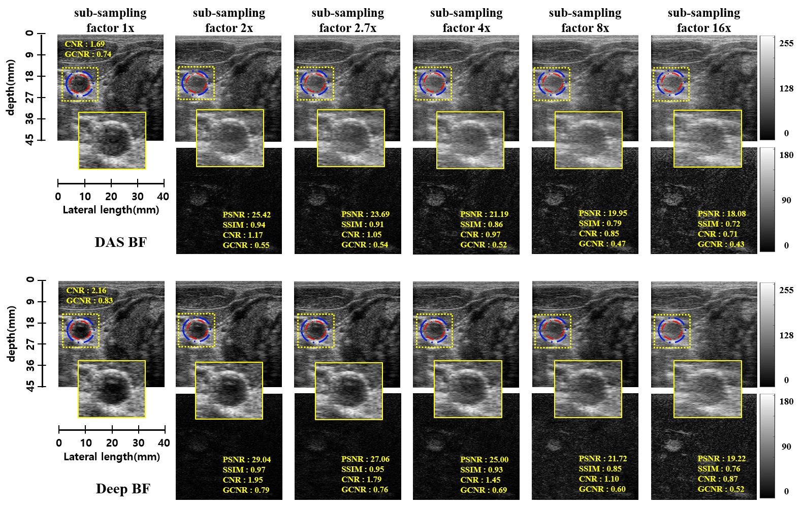
(a) Variable sampling scheme

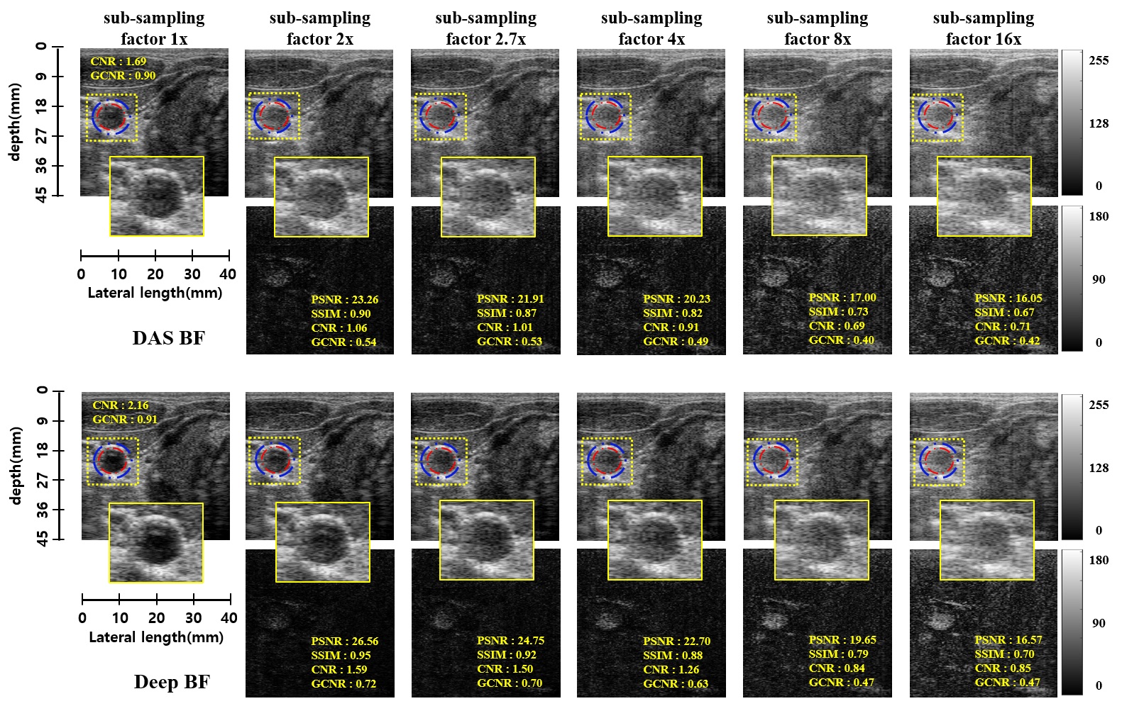
(b) Fixed sampling scheme

Figure 4: Reconstruction results of standard DAS beam-former and the proposed method for carotid region with respect to two subsampling scheme.

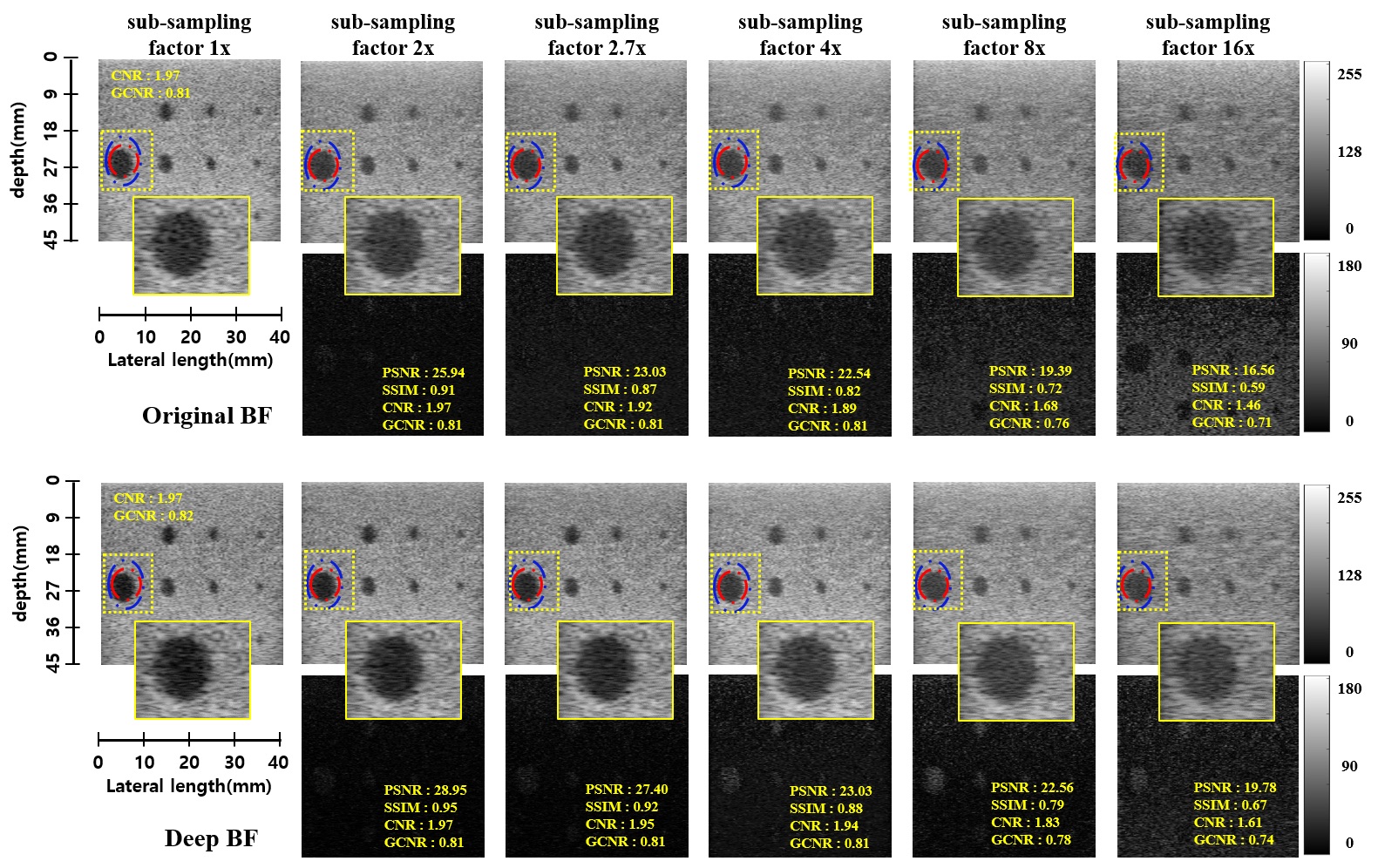
(a) Variable sampling scheme

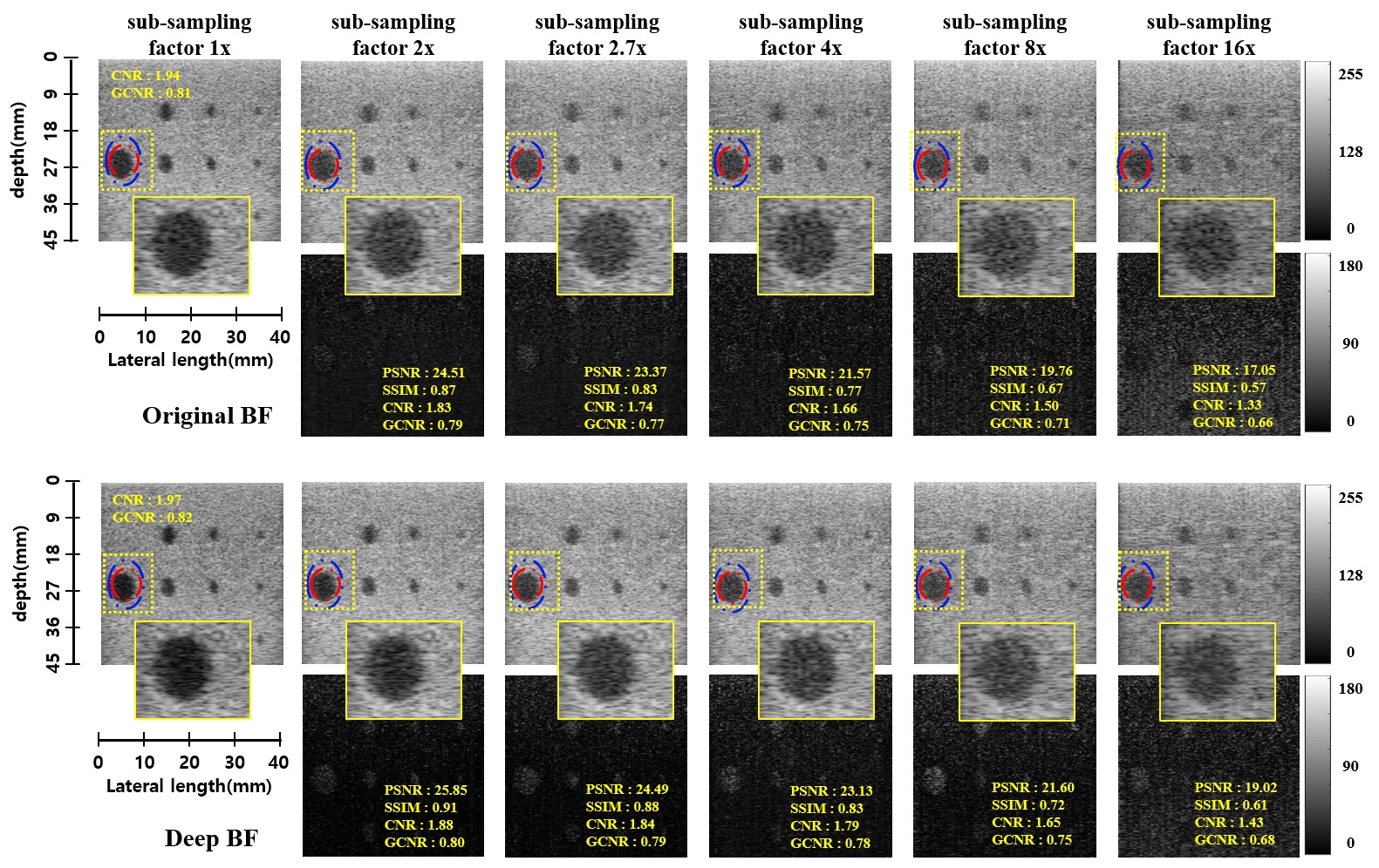
(b) Fixed sampling scheme

Figure 5: Reconstruction results of standard DAS beam-former and proposed method for phantom with respect to two subsampling scheme.

IV Experimental Results

Figs. 4(a)(b) show the results of two in vivo examples for $64$, $32$, $24$, $16$, $8$ and $4$ Rx-channels down-sampling schemes using (a) variable sampling scheme and (b) fixed sampling scheme. Since 64 channels are used as a full sampled data, this corresponds to $1\times,2\times,2.7\times,4\times,8\times$ and $16\times$ acceleration. The images are generated using the proposed DeepBF and the standard DAS beam-former method. Our method significantly improves the visual quality of the US images by estimating the correct dynamic range and eliminating artifacts for both sampling schemes. From difference images in both figures, it is evident that under fixed down-sampling scheme, the quality degradation of images is higher than the variable sampling scheme, but the relative improvement in both schemes using the proposed method is nearly the same. Note that the proposed method successfully reconstruction both the near and the far field regions with equal efficacy, and only minor structural details are imperceivable. Furthermore, it is remarkable that the CNR and GCNR values are significantly improved by the DeepBF even for the fully sampled case (eg. from 1.69 to 2.16 in CNR and from 0.74 to 0.83 in GCNR for the case of variable sampling scheme), which clearly shows the advantages of the proposed method.

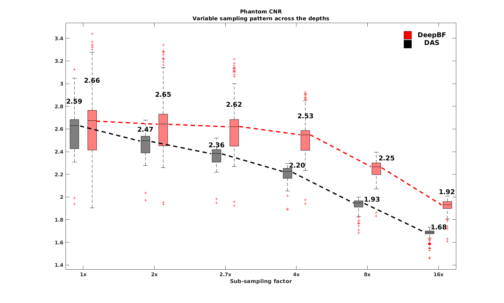
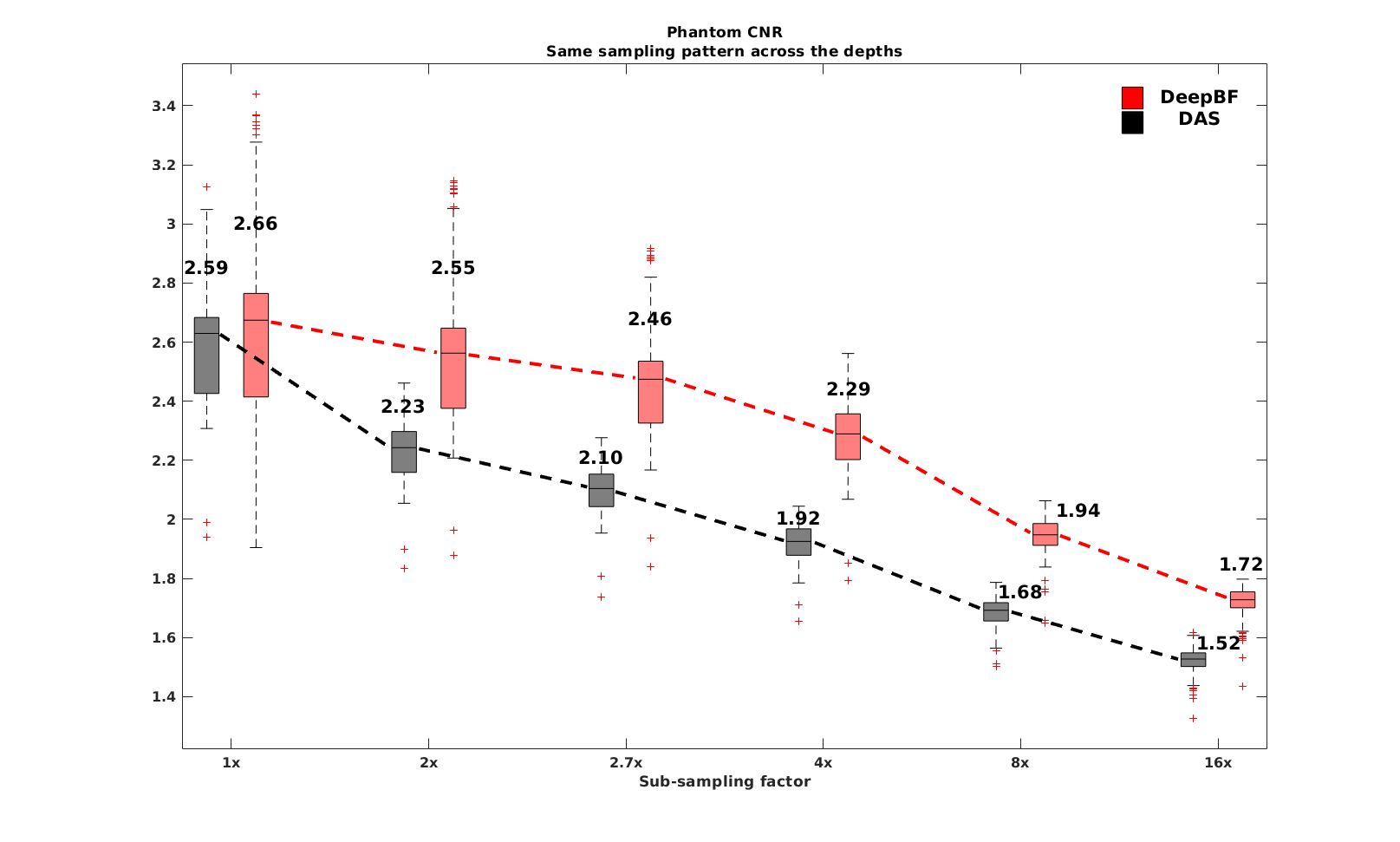
(a) CNR value distribution

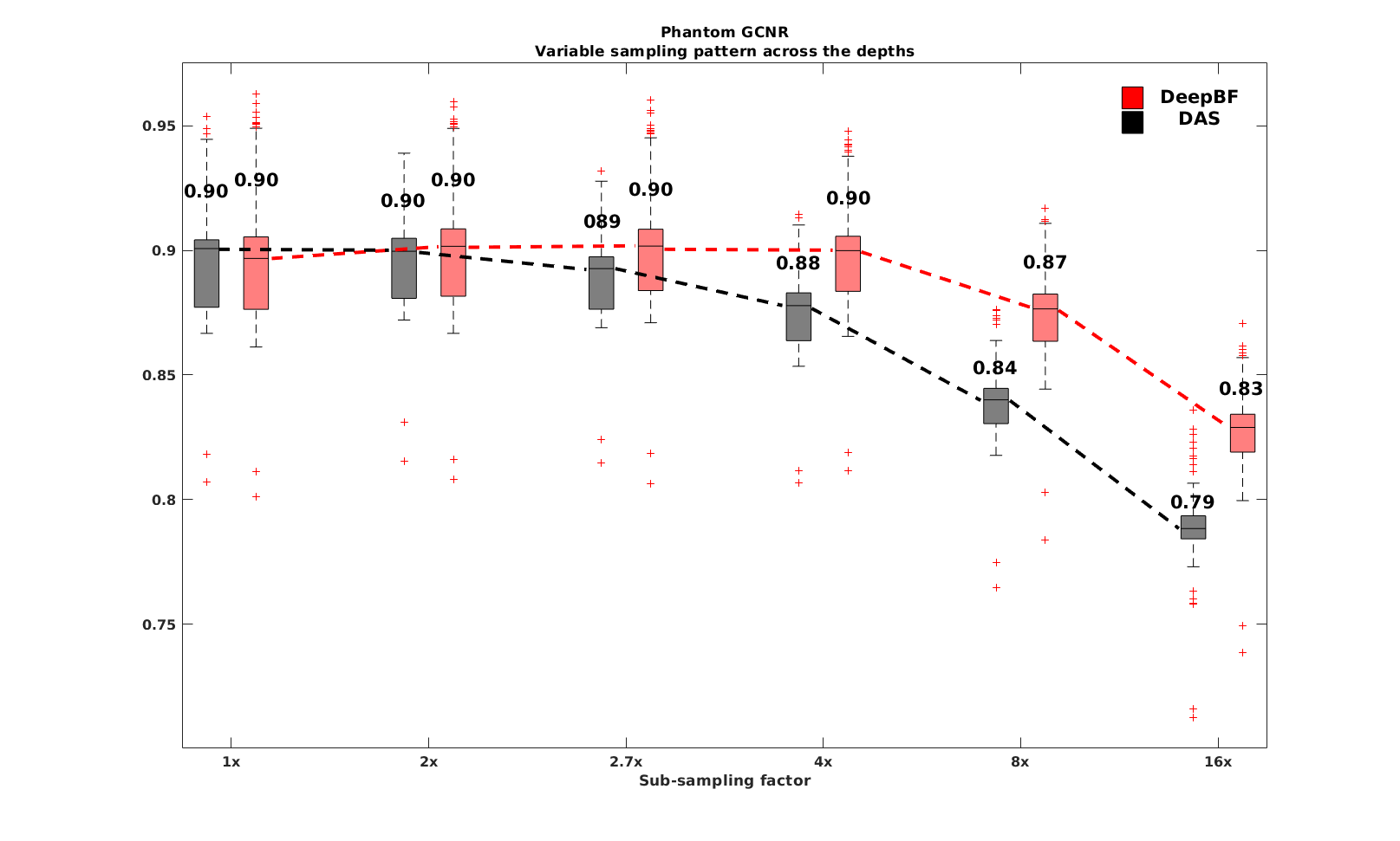
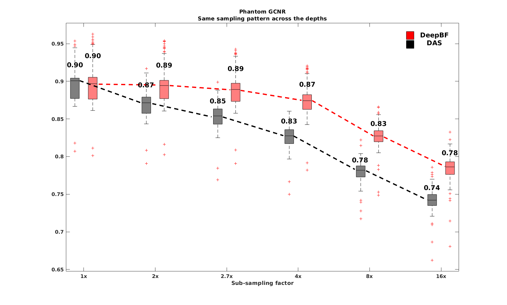
(b) GCNR value distribution

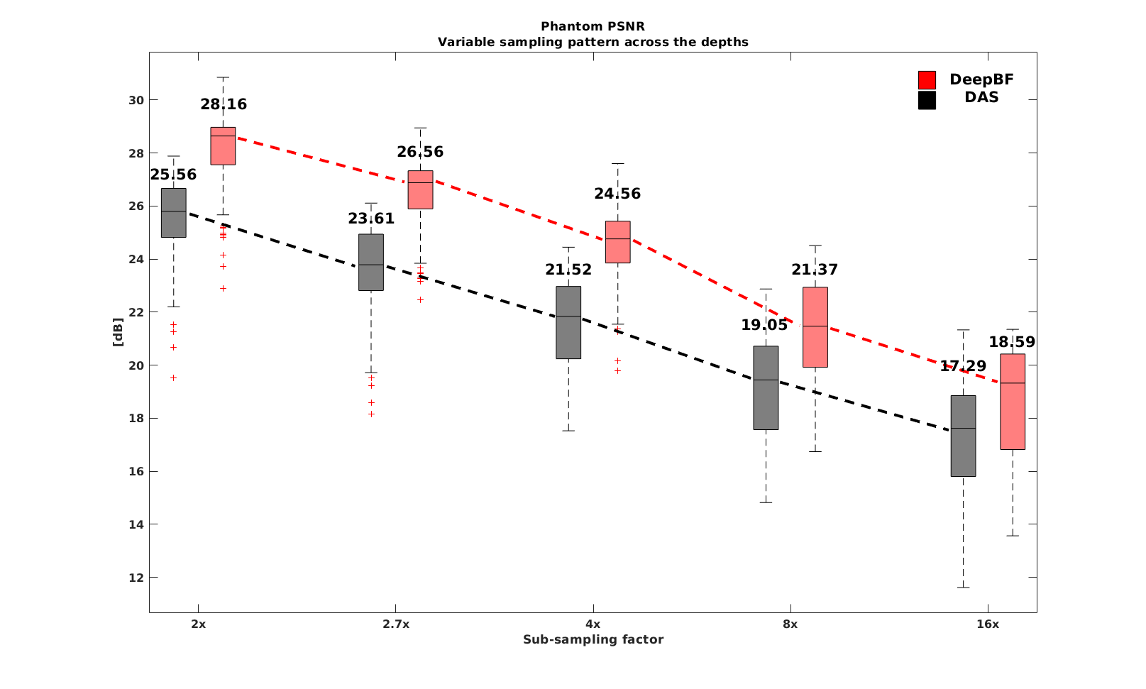
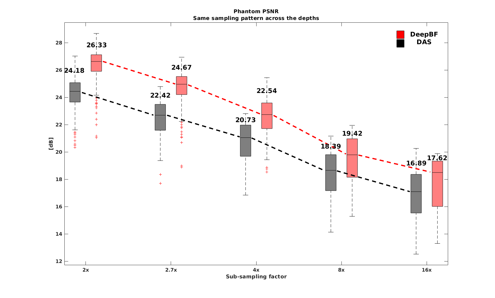
(c) PSNR value distribution

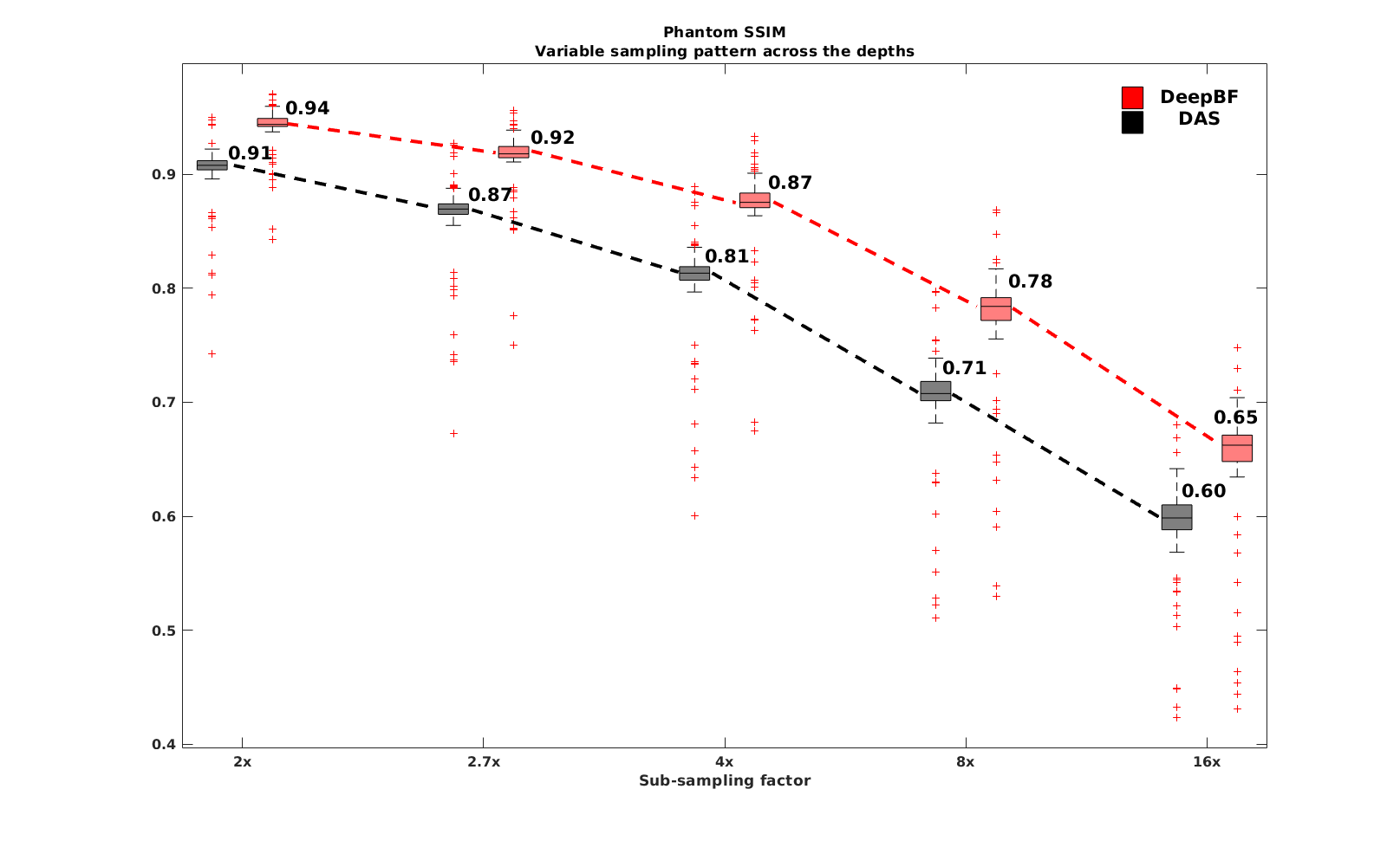
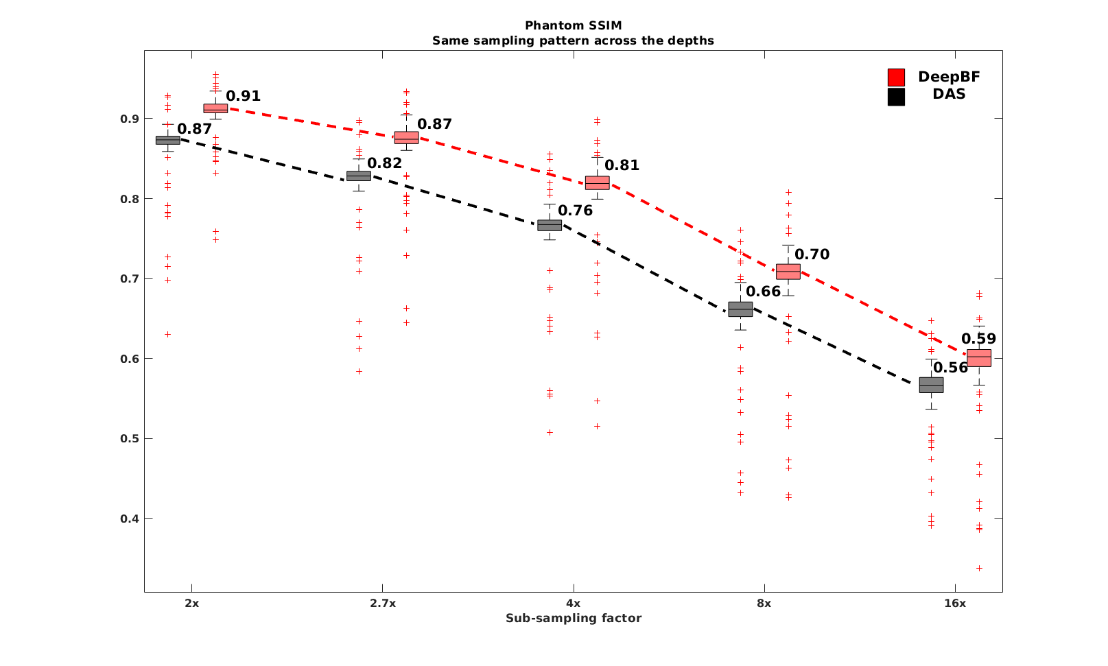
(d) SSIM value distribution

Figure 6: Quantitative comparison using phantom data on different down-sampling schemes: (first column) variable sampling pattern cross the depth, (second column) fixed sampling pattern cross the depth

Fig. 5(a)(b) illustrate two representative examples of phantom data at $1\times,2\times,2.7\times,4\times,8\times$ and $16\times$ acceleration. By harnessing the spatio-temporal (multi-depth and multi-line) learning, the proposed CNN-based beam-former successfully reconstructs the images with good quality in all down-sampling schemes. CNN automatically identifies the missing RF data and approximates it with available neighboring information. Note that the network was trained on variable sampling scheme only; however, the relative improvement in both schemes in test phase is nearly the same for both sampling schemes. This shows the generalization power of the proposed method.

TABLE II: Performance statistics on in vivo data for variable sampling pattern

DSR	CNR		GCNR		PSNR (dB)		SSIM
	DAS	DeepBF	DAS	DeepBF	DAS	DeepBF	DAS	DeepBF
1	1.38	1.45	0.64	0.66	$\infty$	$\infty$	1	1
2	1.33	1.47	0.63	0.66	24.59	27.38	0.89	0.95
2.7	1.3	1.44	0.62	0.66	23.15	25.54	0.86	0.92
4	0.25	1.38	0.6	0.64	21.68	23.55	0.81	0.87
8	1.18	1.26	0.58	0.6	19.99	21.03	0.74	0.77
16	1.12	1.17	0.56	0.58	18.64	19.22	0.67	0.69

TABLE III: Performance statistics on in vivo data for fixed sampling pattern

Subsampling ratio	CNR		GCNR		PSNR (dB)		SSIM
	DAS	DeepBF	DAS	DeepBF	DAS	DeepBF	DAS	DeepBF
1	1.38	1.45	0.64	0.66	0	0	1	1
2	1.21	1.37	0.6	0.64	22.69	24.91	0.85	0.9
2.7	1.15	1.31	0.58	0.63	21.36	23.18	0.8	0.86
4	1.1	1.22	0.56	0.6	20.08	21.38	0.75	0.8
8	1.04	1.11	0.54	0.56	18.63	19.09	0.68	0.7
16	1.02	1.08	0.53	0.55	17.84	17.84	0.63	0.64

We compared the CNR, GCNR, PSNR, and SSIM distributions of reconstructed B-mode images obtained from $188$ phantom test frames. In Fig. 6(a), for the variable sub-sampling scheme, the proposed method achieved average CNR values of $2.66$, $2.65$, $2.62$, $2.53$, $2.25$, and $1.92$ in $64$, $32$, $24$, $16$, $8$ and $4$ Rx-channels down-sampling schemes, respectively, which are $2.70\%$, $7.29\%$, $11.02\%$, $15.00\%$, $16.58\%$ and $14.29\%$ higher than the standard DAS results. Whereas, on fixed sampling scheme, the proposed method achieved average CNR values of $2.66$, $2.55$, $2.46$, $2.29$, $1.94$, and $1.72$ in $64$, $32$, $24$, $16$, $8$ and $4$ Rx-channels down-sampling schemes, respectively. These values are $2.70\%$, $14.35\%$, $17.14\%$, $19.27\%$, $15.48\%$ and $13.16\%$ higher than the standard DAS results.

To test the robustness of our method we also evaluated the GCNR for all images. Fig. 6(b) compare the GCNR distributions for in vivo and phantom data. Compared to standard DAS, the proposed deep beamformer showed significant improvement for both sampling schemes at various subsampling factors. Note that the GCNR of DeepBF images exhibit graceful degradation with respect to the subsampling factors in contrast to the DAS beamformer. In fact, until $4\times$ subsampling, no performance degradation in GCNR was observed. This again shows the robustness of the method.

CNR, and GCNR, are the intensity differences measure for local regions, whereas the PSNR is the global intensity difference. Fig. 6(c) compare the PSNR distributions. To calculate the PSNR, images generated from $64$ Rx-channels were considered as a reference image for all sampling schemes. Compared to standard DAS, using variable subsampling patterns, the proposed deep learning method showed $2.6$dB, $2.95$dB, $3.04$dB, $2.32$dB, and $1.3$dB improvement on average for $32$, $24$, $16$, $8$ and $4$ Rx-channels down-sampling ratios (DSRs), respectively. Similar improvement was seen for the fixed downsampling scheme. Whereas, for fixed subsampling patterns, the proposed deep learning method showed $2.15$dB, $2.25$dB, $1.81$dB, $1.03$dB, and $0.73$dB improvement on average for $32$, $24$, $16$, $8$ and $4$ Rx-channels down-sampling schemes, respectively.

Another important measure of similarity is the structure similarity measure (SSIM). The higher SSIM means good recovery of detailed features of the image. To calculate the SSIM, images generated using $64$ Rx-channels were considered as reference images for all sampling schemes. As shown in Fig. 6(d) the proposed method shows significantly higher SSIM values for both sampling schemes.

We also compared the CNR, GCNR, PSNR, and SSIM distributions of reconstructed B-mode images obtained from $360$ in-vivo test frames. Table II and  III showed that the proposed deep beamformer consistently outperformed the standard DAS beamformer for all subsampling scheme and ratio.

One big advantage of ultrasound image modality is it run-time imaging capability, which require fast reconstruction time. Another important advantage of the proposed method is the run-time complexity. Although training required $40$ hours for $200$ epochs using MATLAB, once training was completed, the reconstruction time for the proposed deep learning method is not very long. The average reconstruction time for each depth planes is around $9.8$ (milliseconds), which could be easily reduce by optimized implementation and reconstruction of multiple depth planes in parallel.

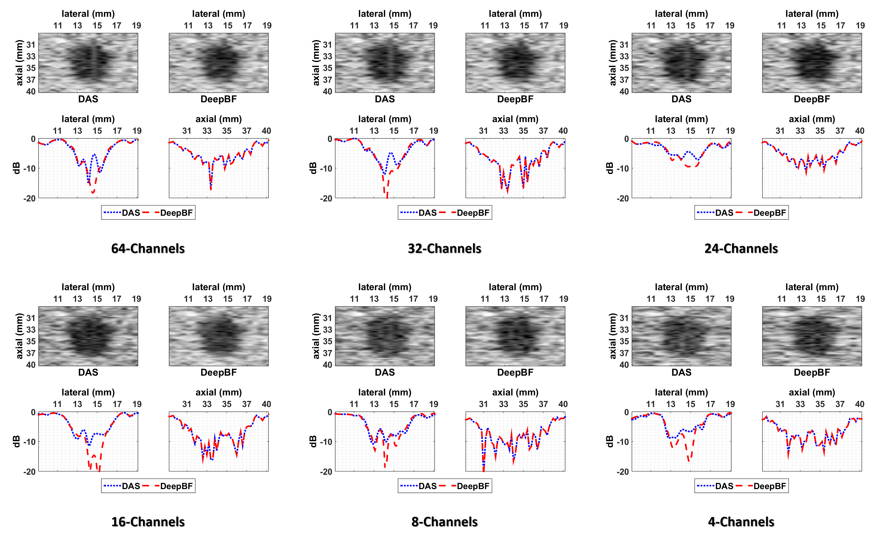
(a) Phantom $6$ mm diameter anechoic cyst at $34$ mm from various RF sub-sampling rate.

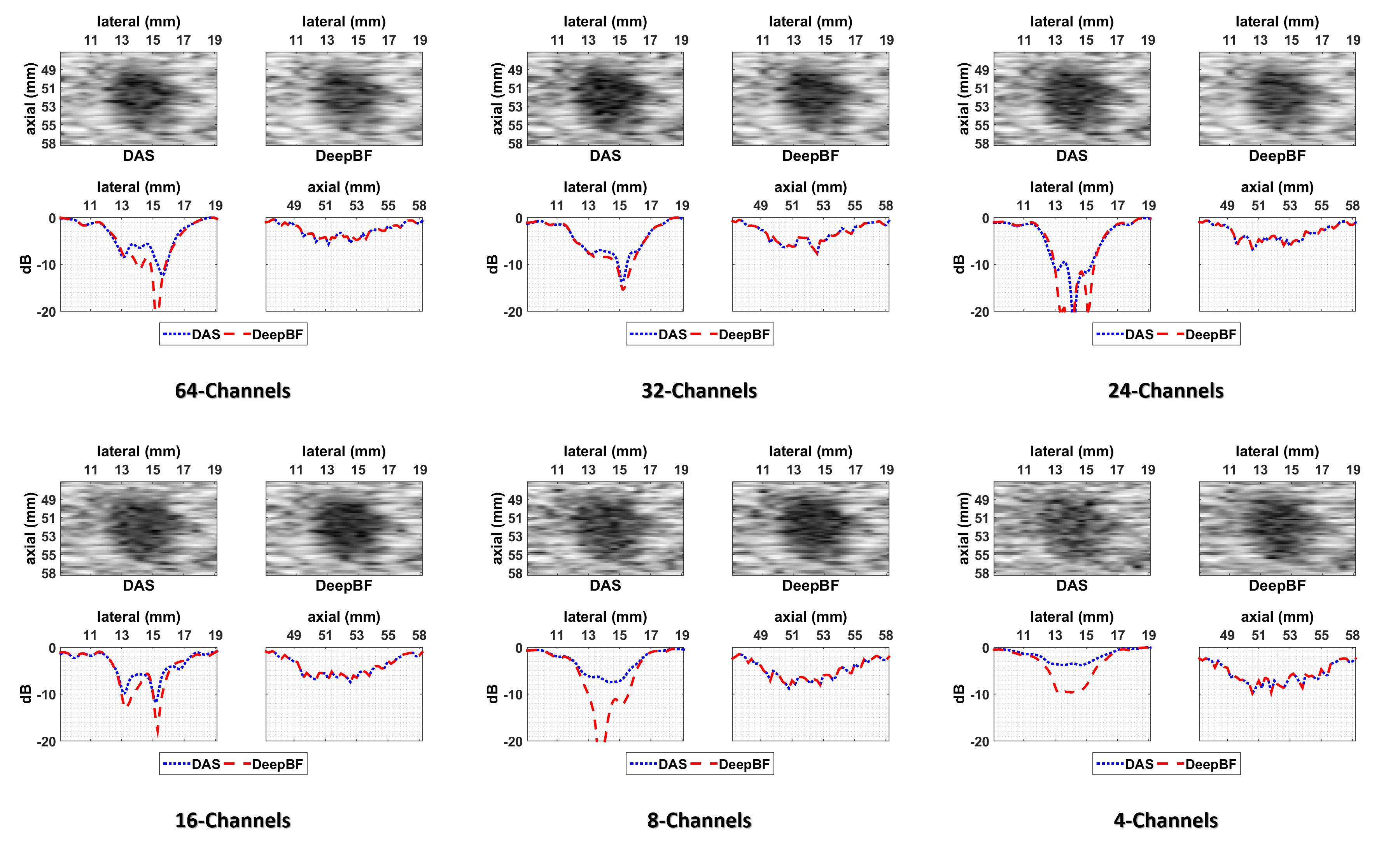
(b) Phantom $6$ mm diameter anechoic cyst at $52$ mm from various RF sub-sampling rate.

Figure 7: Lateral and axial profiles through the center of the phantom anechoic cyst using DAS and DeepBF on random sampling across depth. Images are shown with a $60$ dB dynamic range.

V Discussion

We have designed a robust system which exploits the significant redundancies in the RF domains, which results in improved GCNR. It is noteworthy that thanks to the exponentially increasing expressiveness of deep networks, for the first time a single universal deep beamformer trained using a purely data-driven way that can generate significantly improved images over widely varying aperture and channel sub-sampling patterns. Moreover, CNR, GCNR, PSNR, and SSIM were significantly improved over standard DAS method. Note that the proposed method efficaciously generate the better quality image from as little as only $6.25$% RF-data.

In Fig 7, we compared lateral and axis profiles through the center of the two phantom anechoic cysts using DAS and DeepBF methods. In particular, two anechoic cysts of $6$mm diameter scanned from the depth of $34$mm and $52$mm and B-mode images were obtained for random sampling scheme on $1\times$,$2\times$,$2.7\times$,$4\times$,$8\times$, and $16\times$ sub-sampling factors using DAS and our DeepBF. From the figures it can be seen that under all sampling schemes, on the boundary of cysts the proposed method show sharp changes in the pixel intensity with respect to the lateral position in the image. Although the axial profile shows similar trend to DAS, the average relative shift in the pixel intensity is constant for all sub-sampling factors, which means their is no significant degradation of axial resolution in sub-sampled images. The different resolution improvement between lateral and axial directions in the proposed method may be due to our training scheme in (11), which only consider the three adjacent depth planes as input and average out the dependency with respect to $n$. The depth dependent training scheme may be a solution for this, which will be investigated in other publications.

Note that our CNN is trained on full sampled ($64$-Rx) data, but surprisingly lateral resolution in DeepBF images is much better than the ($64$-Rx) images obtained from standard DAS method. This super resolution effect is prominent for both cysts obtained from different depths and the results are consistent cross the all sub-sampling factors. This is consistent with our observation on the CNR and GCNR improvement on the full sampled data. We believe that this is originated from the synergistic learning from multiple data set, which is not possible from analytic form of standard DAS beamformer.

VI Conclusion

In this paper, we presented a universal deep learning-based beamformer to generate high-quality B-mode ultrasound image from various rate of sub-sampled channel data. The proposed method is purely a data-driven method which exploits the spatio-temporal redundancies in the raw RF data, which help in generating improved quality B-mode images using fewer Rx channels. The proposed method improved the contrast of B-modes images by preserving the dynamic range and structural details of the RF signal in both the phantom and in-vivo scans. Due to the exponential large expressiveness of the deep neural network, our novel universal deep beamformer can efficiently learn various mappings from RF measurements, and exhibits superior image quality for all sub-sampling rates. Furthermore, the network was also used for the fully sampled RF data to significantly improve the image contrast and resolution. This super-resolution effects of neural network is shown in both phantom and in-vivo images. Therefore, this method can be an important platform for RF sub-sampled US imaging.

References

- [1] Fink, M. Time reversal of ultrasonic fields. i. basic principles. IEEE Transactions on Ultrasonics, Ferroelectrics, and Frequency Control 39, 555–566 (1992).
- [2] Wu, F., Thomas, J. . & Fink, M. Time reversal of ultrasonic fields. il. experimental results. IEEE Transactions on Ultrasonics, Ferroelectrics, and Frequency Control 39, 567–578 (1992).
- [3] Viola, F. & Walker, W. F. Adaptive signal processing in medical ultrasound beamforming. In IEEE Ultrasonics Symposium, 2005., vol. 4, 1980–1983 (2005).
- [4] Capon, J. High-resolution frequency-wavenumber spectrum analysis. Proceedings of the IEEE 57, 1408–1418 (1969).
- [5] Vignon, F. & Burcher, M. R. Capon beamforming in medical ultrasound imaging with focused beams. IEEE Transactions on Ultrasonics, Ferroelectrics, and Frequency Control 55, 619–628 (2008).
- [6] Kim, K., Park, S., Kim, J., Park, S. & Bae, M. A fast minimum variance beamforming method using principal component analysis. IEEE Transactions on Ultrasonics, Ferroelectrics, and Frequency Control 61, 930–945 (2014).
- [7] Chen, W., Zhao, Y. & Gao, J. Improved capon beamforming algorithm by using inverse covariance matrix calculation. In IET International Radar Conference 2013, 1–6 (2013).
- [8] Nilsen, C. . C. & Hafizovic, I. Beamspace adaptive beamforming for ultrasound imaging. IEEE Transactions on Ultrasonics, Ferroelectrics, and Frequency Control 56, 2187–2197 (2009).
- [9] Deylami, A. M. & Asl, B. M. A fast and robust beamspace adaptive beamformer for medical ultrasound imaging. IEEE Transactions on Ultrasonics, Ferroelectrics, and Frequency Control 64, 947–958 (2017).
- [10] Jensen, A. C. & Austeng, A. An approach to multibeam covariance matrices for adaptive beamforming in ultrasonography. IEEE Transactions on Ultrasonics, Ferroelectrics, and Frequency Control 59, 1139–1148 (2012).
- [11] Jensen, A. C. & Austeng, A. The iterative adaptive approach in medical ultrasound imaging. IEEE Transactions on Ultrasonics, Ferroelectrics, and Frequency Control 61, 1688–1697 (2014).
- [12] Schretter, C. et al. Ultrasound imaging from sparse RF samples using system point spread functions. IEEE Transactions on Ultrasonics, Ferroelectrics, and Frequency Control 65, 316–326 (2018).
- [13] Yoon, Y. H., Khan, S., Huh, J., Ye, J. C. et al. Efficient b-mode ultrasound image reconstruction from sub-sampled rf data using deep learning. IEEE transactions on medical imaging (2018).
- [14] Tur, R., Eldar, Y. C. & Friedman, Z. Innovation rate sampling of pulse streams with application to ultrasound imaging. IEEE Transactions on Signal Processing 59, 1827–1842 (2011).
- [15] Wagner, N., Eldar, Y. C. & Friedman, Z. Compressed beamforming in ultrasound imaging. IEEE Transactions on Signal Processing 60, 4643–4657 (2012).
- [16] Chernyakova, T. & Eldar, Y. Fourier-domain beamforming: the path to compressed ultrasound imaging. IEEE transactions on ultrasonics, ferroelectrics, and frequency control 61, 1252–1267 (2014).
- [17] Kang, E., Min, J. & Ye, J. C. A deep convolutional neural network using directional wavelets for low-dose x-ray ct reconstruction. Medical Physics 44 (2017).
- [18] Kang, E., Chang, W., Yoo, J. & Ye, J. C. Deep convolutional framelet denosing for low-dose CT via wavelet residual network. IEEE Transactions on Medical Imaging 37, 1358–1369 (2018).
- [19] Chen, H. et al. Low-dose CT via convolutional neural network. Biomedical Optics Express 8, 679–694 (2017).
- [20] Adler, J. & Öktem, O. Learned primal-dual reconstruction. IEEE Transactions on Medical Imaging (in press) (2018).
- [21] Wolterink, J. M., Leiner, T., Viergever, M. A. & Išgum, I. Generative adversarial networks for noise reduction in low-dose CT. IEEE Transactions on Medical Imaging 36, 2536–2545 (2017).
- [22] Jin, K. H., McCann, M. T., Froustey, E. & Unser, M. Deep convolutional neural network for inverse problems in imaging. IEEE Transactions on Image Processing 26, 4509–4522 (2017).
- [23] Han, Y. & Ye, J. C. Framing U-Net via deep convolutional framelets: Application to sparse-view CT. IEEE Transactions on Medical Imaging 37, 1418–1429 (2018).
- [24] Wang, S. et al. Accelerating magnetic resonance imaging via deep learning. In Biomedical Imaging (ISBI), 2016 IEEE 13th International Symposium on, 514–517 (IEEE, 2016).
- [25] Hammernik, K. et al. Learning a variational network for reconstruction of accelerated MRI data. Magnetic resonance in medicine 79, 3055–3071 (2018).
- [26] Schlemper, J., Caballero, J., Hajnal, J. V., Price, A. N. & Rueckert, D. A deep cascade of convolutional neural networks for dynamic MR image reconstruction. IEEE Transactions on Medical Imaging 37, 491–503 (2018).
- [27] Zhu, B., Liu, J. Z., Cauley, S. F., Rosen, B. R. & Rosen, M. S. Image reconstruction by domain-transform manifold learning. Nature 555, 487 (2018).
- [28] Lee, D., Yoo, J., Tak, S. & Ye, J. Deep residual learning for accelerated MRI using magnitude and phase networks. IEEE Transactions on Biomedical Engineering (2018).
- [29] Allman, D., Reiter, A. & Bell, M. A. L. A machine learning method to identify and remove reflection artifacts in photoacoustic channel data. In 2017 IEEE International Ultrasonics Symposium (IUS), 1–4 (2017).
- [30] Luchies, A. C. & Byram, B. C. Deep neural networks for ultrasound beamforming. IEEE transactions on medical imaging 37, 2010–2021 (2018).
- [31] Feigin, M., Freedman, D. & Anthony, B. W. A deep learning framework for single sided sound speed inversion in medical ultrasound. arXiv preprint arXiv:1810.00322 (2018).
- [32] Perdios, D., Besson, A., Arditi, M. & Thiran, J.-P. A deep learning approach to ultrasound image recovery. In 2017 IEEE International Ultrasonics Symposium (IUS), 1–4 (IEEE, 2017).
- [33] Zhou, Z. et al. High spatial-temporal resolution reconstruction of plane-wave ultrasound images with a multichannel multiscale convolutional neural network. IEEE transactions on ultrasonics, ferroelectrics, and frequency control (2018).
- [34] Gasse, M. et al. High-quality plane wave compounding using convolutional neural networks. IEEE transactions on ultrasonics, ferroelectrics, and frequency control 64, 1637–1639 (2017).
- [35] Senouf, O. et al. High frame-rate cardiac ultrasound imaging with deep learning. In Frangi, A. F., Schnabel, J. A., Davatzikos, C., Alberola-López, C. & Fichtinger, G. (eds.) Medical Image Computing and Computer Assisted Intervention – MICCAI 2018, 126–134 (Springer International Publishing, Cham, 2018).
- [36] Vedula, S. et al. High quality ultrasonic multi-line transmission through deep learning. In Knoll, F., Maier, A. & Rueckert, D. (eds.) Machine Learning for Medical Image Reconstruction, 147–155 (Springer International Publishing, Cham, 2018).
- [37] Long, X., Salehin, S. M. A. & Abhayapala, T. D. Robust capon beamformer with frequency smoothing applied to medical ultrasound imaging. In 2014 IEEE Workshop on Statistical Signal Processing (SSP), 173–176 (2014).
- [38] Rolnick, D. & Tegmark, M. The power of deeper networks for expressing natural functions. arXiv preprint arXiv:1705.05502 (2017).
- [39] Telgarsky, M. Benefits of depth in neural networks. In Conference on Learning Theory, 1517–1539 (2016).
- [40] Arora, R., Basu, A., Mianjy, P. & Mukherjee, A. Understanding deep neural networks with rectified linear units. arXiv preprint arXiv:1611.01491 (2016).
- [41] Brandwood, D. H. A complex gradient operator and its application in adaptive array theory. IEE Proceedings F - Communications, Radar and Signal Processing 130, 11–16 (1983).
- [42] Synnevag, J. F., Austeng, A. & Holm, S. Adaptive beamforming applied to medical ultrasound imaging. IEEE Transactions on Ultrasonics, Ferroelectrics, and Frequency Control 54, 1606–1613 (2007).
- [43] Synnevag, J., Austeng, A. & Holm, S. Benefits of minimum-variance beamforming in medical ultrasound imaging. IEEE Transactions on Ultrasonics, Ferroelectrics, and Frequency Control 56, 1868–1879 (2009).
- [44] Matrone, G., Savoia, A., Caliano, G. & Magenes, G. The delay multiply and sum beamforming algorithm in ultrasound b-mode medical imaging. IEEE Trans. Med. Imaging 34, 940–949 (2015).
- [45] Matrone, G., Ramalli, A., Savoia, A. S., Tortoli, P. & Magenes, G. High frame-rate, high resolution ultrasound imaging with multi-line transmission and filtered-delay multiply and sum beamforming. IEEE transactions on medical imaging 36, 478–486 (2017).
- [46] Matrone, G., Savoia, A. S., Caliano, G. & Magenes, G. Depth-of-field enhancement in filtered-delay multiply and sum beamformed images using synthetic aperture focusing. Ultrasonics 75, 216–225 (2017).
- [47] Cohen, R. & Eldar, Y. C. Sparse convolutional beamforming for ultrasound imaging. arXiv preprint arXiv:1805.05101 (2018).
- [48] Vedaldi, A. & Lenc, K. Matconvnet: Convolutional neural networks for matlab. In Proceedings of the 23rd ACM international conference on Multimedia, 689–692 (ACM, 2015).
- [49] Glorot, X. & Bengio, Y. Understanding the difficulty of training deep feedforward neural networks. In Proceedings of the Thirteenth International Conference on Artificial Intelligence and Statistics, 249–256 (2010).
- [50] Rangayyan, R. M. Biomedical Image Analysis. Biomedical Engineering (CRC Press, Boca Raton, Florida, 2005).
- [51] Rodriguez-Molares, A. et al. The generalized contrast-to-noise ratio (2018).
- [52] Wang, Z., Bovik, A. C., Sheikh, H. R. & Simoncelli, E. P. Image quality assessment: from error visibility to structural similarity. IEEE Transactions on Image Processing 13, 600–612 (2004).