Projections of determinantal point processes

Abstract

Let $\mathbf{x}=\{x^{(1)},\dots,x^{(n)}\}$ be a space filling-design of $n$ points defined in $\left[0{,}1\right]^{d}$. In computer experiments, an important property seeked for $\mathbf{x}$ is a nice coverage of $\left[0{,}1\right]^{d}$. This property could be desirable as well as for any projection of $\mathbf{x}$ onto $\left[0{,}1\right]^{\iota}$ for $\iota<d$ . Thus we expect that $\mathbf{x}_{I}=\{x_{I}^{(1)},\dots,x_{I}^{(n)}\}$, which represents the design $\mathbf{x}$ with coordinates associated to any index set $I\subseteq\{1,\dots,d\}$, remains regular in $\left[0{,}1\right]^{\iota}$ where $\iota$ is the cardinality of $I$. This paper examines the conservation of nice coverage by projection using spatial point processes, and more specifically using the class of determinantal point processes. We provide necessary conditions on the kernel defining these processes, ensuring that the projected point process $\mathbf{X}_{I}$ is repulsive, in the sense that its pair correlation function is uniformly bounded by 1, for all $I\subseteq\{1,\dots,d\}$. We present a few examples, compare them using a new normalized version of Ripley’s function. Finally, we illustrate the interest of this research for Monte-Carlo integration.

Introduction

Space-filling designs, e.g. Latin hypercubes [17, 20], low discrepancy sequences [[, e.g.]]Halton64,Sobol67, are popular methods in computer experiments. These computational methods are becoming unavoidable to simulate complex phenomena [[, e.g.]Chapter 5]Santneretal13. A space-filling design corresponds to a set $\mathbf{x}=\{x^{(1)},\dots,x^{(n)}\}$ of $n$ points generated in a bounded domain, for instance $\left[0{,}1\right]^{d}$ in the following. Usually, the dimension $d$ represents the number of factors (or covariates) on which the numerical code depends. The $k$th coordinates of points from $\mathbf{x}$ then represent the values of the $k$th factor. Intuitively, points issued from a space filling-design tend to regularly cover the domain $\left[0{,}1\right]^{d}$. The quality of this coverage can be a priori evaluated by standard criteria such as maximin distance or $L^{2}$ discrepancy [[, see e.g.]]Owen13.

Frequently in computer experiments, some factors are a posteriori found to be inactive [[, see]and references therein]Sunetal19. If the experiment is to be performed again, an inactive factor must be discarded to avoid numerical errors and to decrease complexity. But if $k$ factors are discarded, the experimental space-filling design should be done again, this time on $\left[0{,}1\right]^{d-k}$. This induces a new complexity and is expensive. A cheaper strategy is to keep the first space-filling design, but use its projection onto $\left[0{,}1\right]^{d-k}$ by discarding the adequate factors (or coordinates). However, the projected points should provide a good coverage of $\left[0{,}1\right]^{d-k}$. Therefore, an additional property of the initial space-filling design should be the conservation of the “nice coverage” property for any subsets of the coordinates.

This additional property has already been considered in the literature for low discrepancy type designs [[, see e.g.]]Sunetal19. Our work in contrast considers spatial point processes as experimental designs. For the question we address, we set $\mathbf{x}_{I}=\{x_{I}^{(1)},\dots,x_{I}^{(n)}\}$ to be the design obtained from the design $\mathbf{x}$ by keeping the factors (coordinates) indexed by the index set $I\subseteq\{1,\dots,d\}$. For example, when $I=\{1,\dots,d-1\}$, $\mathbf{x}_{I}$ corresponds to the set $\mathbf{x}$ where the $d$th coordinate of each point is discarded. We let $\mathbf{X}$ to be the spatial point process generating $\mathbf{x}$ and $\mathbf{X}_{I}$ the process generating $\mathbf{x}_{I}$. In the spatial statistics literature, the pair correlation function (denoted by $g$) is the most standard way for characterizing the pairwise dependence between points, see e.g. [18]: $g_{\mathbf{X}}(x,y)$ measures the probability to observe a pair of distinct points at $(x,y)$, normalized by the same probability under the Poisson case, i.e. under the situation where there is no interaction between points (see Section 1 for a more formal definition of the pair correlation function). A point process for which $g_{\mathbf{X}}<1$, i.e. $g_{\mathbf{X}}(x,y)<1$ for all $x,y\in\left[0{,}1\right]^{d}$ is qualified as a repulsive point process in [18, 12]. Thanks to repulsiveness, points of a repulsive point process tend to cover more regularly the space than a Poisson point process does. For the application to computer experiments which motivates our study, we intend to develop point process models which are repulsive in all directions, i.e. spatial point processes $\mathbf{X}$ such that $g_{\mathbf{X}_{I}}<1$ for all $I\subseteq\{1,\dots,d\}$.

Several classes of spatial point processes are able to generate regular patterns. Among them, Matérn hard-core processes [28], Gibbs point processes [18, 6] or determinantal point processes [14] are appealing for many applications. In particular Gibbs point processes have been considered to generate space-filling designs in [8, 7]. The authors build a specific Gibbs model by parameterizing its Papangelou conditional intensity as a Strauss hard-core model with constraints on the marginals. The resulting patterns look regular and the points cover regularly the space. However, Gibbs point processes have the drawback of not having their moments available in a closed form. In particular, the intensity as well as the pair correlation function [[, see e.g.]]Dereudre19 are not available analytically. Even worse, using Monte-Carlo simulations in [12] show that the pair correlation function of Strauss hard-core models are not uniformly bounded by 1 . Although Matérn hard-core processes are more tractable, their pair correlation function suffer from the same problem [[, see]]Teichmannetal13.

Determinantal point processes (DPPs for short) have been introduced in [15] as “fermion” processes to model the position of particles that repel each other. This class of processes is known for very appealing properties, in particular for its tractability: explicit expressions for the intensity functions are available. Therefore, a growing attention has been paid to DPPs from a theoretical point of view [[, e.g.]]Soshnikov00, ShiraiTakahashi03,Houghetal09,Decreusefondetal16, and more recently in the statistics community [14, 2]. In particular, one of the main characteristics of a DPP is that, by construction, its pair correlation function is uniformly bounded by 1. DPPs are defined through a kernel $K:B\times B\to\mathbb{C}$ which characterizes the distribution of $\mathbf{X}$ and thus which characterizes also its moments. The main result of this paper concerns necessary conditions (expressed by Assumption ($H[I]$)) on the form of kernel $K$ to ensure that the projected pattern $\mathbf{X}_{I}$ remains repulsive, i.e. such that $g_{\mathbf{X}_{I}}<1$.

The paper is organized as follows. Section 1 contains a brief background on spatial point processes and in particular on DPPs. Section 2 deals with the statistical description of the projected point process $\mathbf{X}_{I}$. In particular we provide a closed form for the pair correlation $g_{\mathbf{X}_{I}}$ when $\mathbf{X}$ is a DPP defined on $\left[0{,}1\right]^{d}$ with kernel $K$ satisfying a separability assumption. Examples of models satisfying this separability condition are presented and discussed in Section 3. They are compared using an original summary statistic, defined as a normalized version of Ripley’s function [[, see e.g.]]MollerWaagepeterson04 based on the sup norm. We illustrate in Section 4 the interest of the models developed in this research. To mimic situations which occur in computer experiments, we consider the Monte-Carlo integration for $\int_{\left[0{,}1\right]^{\iota}}f_{I}(u)\mathrm{d}u$, for any function $f_{I}:\left[0{,}1\right]^{\iota}\to\mathbb{R}$ and any $I\subseteq\{1,\dots,d\}$ with cardinality $\iota=1,\dots,d$. We demonstrate that the single initial design defined on $\left[0{,}1\right]^{d}$ and its projections can be used to achieve this task efficiently. Proofs of our results are postponed to appendices.

1 Background and notation

1.1 Spatial point processes

A spatial point process $\mathbf{X}$ defined on a Borel set $B\subseteq\mathbb{R}^{d}$ is a locally finite measure on $B$, (for measure theoretical details, see e.g. [18] and references therein) whose realization is of the form $\{x^{(1)},\ldots,x^{(k)}\}\in B^{k}$ where $k$ is the realization of a random variable and the $x^{(i)}$’s represent the events. We assume that $\mathbf{X}$ is simple meaning that two events cannot occur at the same location. Thus, $\mathbf{X}$ is viewed as a locally finite random set.

In most cases, the distribution of a point process $\mathbf{X}$ can be described by its intensity functions $\rho_{\mathbf{X}}^{(k)}:B^{k}\rightarrow\mathbb{R}^{+}$, $k\in\mathbb{N}\setminus\{0\}$. By Campbell Theorem [[, e.g.]]MollerWaagepeterson04, $\rho_{\mathbf{X}}^{(k)}$ is characterized by the following integral representation: for any non-negative measurable function $h:B^{k}\to\mathbb{R}^{+}$

$$\mathbb{E}\Bigg{[} \sum_{x^{(1)},\ldots,x^{(k)}\in\mathbf{X}}^{\neq}h\left(x^{(1)},\ldots,x^{(k)}\right)\Bigg{]}$$

$$=\int_{B^{k}}\rho_{\mathbf{X}}^{(k)}\left(x^{(1)},\ldots,x^{(k)}\right)h\left(x^{(1)},\ldots,x^{(k)}\right)\mathrm{d}x^{(1)}\ldots\mathrm{d}x^{(k)}$$ (1)

where $\neq$ over the summation means that $x^{(1)},\ldots,x^{(k)}~{}$ are pairwise distinct points. Intuitively, for any pairwise distinct points $x^{(1)},\ldots,x^{(k)}\in B$, $\rho_{\mathbf{X}}^{(k)}\left(x^{(1)},\ldots,x^{(k)}\right)\mathrm{d}x^{(1)}\ldots\mathrm{d}x^{(k)}$ is the probability that $\mathbf{X}$ has a point in each of the $k$ infinitesimally small sets around $x^{(1)},\ldots,x^{(k)}$ with volumes $\mathrm{d}x^{(1)},\ldots,\mathrm{d}x^{(k)}$, respectively. When $k=1$, this yields the intensity function and we simply denote it by $\rho_{\mathbf{X}}=\rho_{\mathbf{X}}^{(1)}$. The second order intensity $\rho_{\mathbf{X}}^{(2)}$ is used to define the pair correlation function

$$g_{\mathbf{X}}(x^{(1)},x^{(2)})=\frac{\rho_{\mathbf{X}}^{(2)}(x^{(1)},x^{(2)})}{\rho_{\mathbf{X}}(x^{(1)})\rho_{\mathbf{X}}(x^{(2)})}\,$$ (2)

for pairwise distinct $x^{(1)}$, $x^{(2)}\in B$, and where $g_{\mathbf{X}}(x^{(1)},x^{(2)})$ is set to 0 if $\rho_{\mathbf{X}}(x^{(1)})$ or $\rho_{\mathbf{X}}(x^{(2)})$ is zero. By convention, $\rho_{\mathbf{X}}^{(k)}\left(x^{(1)},\ldots,x^{(k)}\right)$ is set to 0 if $x^{(i)}=x^{(j)}$ for some $i\neq j$. Therefore $g_{\mathbf{X}}(x,x)$ is also set to 0 for all $x\in B$. The pair correlation function (pcf for short) can be used to determine the local interaction between points of $\mathbf{X}$ located at $x$ and $y$: $g_{\mathbf{X}}(x,y)>1$ characterizes positive correlation between the points; $g_{\mathbf{X}}(x,y)=1$ means there is no interaction (typically a Poisson point process); $g_{\mathbf{X}}(x,y)<1$ characterizes negative correlations. A point pattern is often referred to as a repulsive point process, if $g(x,y)<1$ for any $x,y\in B$ [[, e.g.]Sec. 6.5]Illianetal08.

A point process $\mathbf{X}$ with constant intensity function on $B$ is said to be homogeneous. A pcf with constant intensity is said to be invariant by translation (resp. isotropic) if $\rho_{\mathbf{X}}^{(2)}(x^{(1)},x^{(2)})$ depends only on $x^{(2)}-x^{(1)}$ (resp. on $\|x^{(2)}-x^{(1)}\|$ for a norm to be defined).

1.2 Determinantal point processes (DPPs)

In this section, the class of continuous DPPs is introduced. We restrict our attention to DPPs defined on a compact set $B\subset\mathbb{R}^{d}$. A point process $\mathbf{X}$ on $B$ is said to be a DPP on $B$ with kernel $K:B\times B\to\mathbb{C}$ if for any $k\geq 1$ its $k$th order intensity function is given by

$$\rho_{\mathbf{X}}^{(k)}\left(x^{(1)},\ldots,x^{(k)}\right)=\det\left[K\left(x^{(i)},x^{(j)}\right)\right]_{i,j=1}^{k}$$ (3)

and we simply denote by $\mathbf{X}\sim\mathrm{DPP}_{B}(K)$. We assume in this work that $K$ is a continuous covariance function and refer the interested reader to more general situations to [11]. The intensity of $\mathbf{X}$ is given by $\rho_{\mathbf{X}}(x)=K(x,x)$ and its pcf by

$$g_{\mathbf{X}}(x,y)=1-\frac{\left|K(x,y)\right|^{2}}{K(x,x)K(y,y)}.$$ (4)

The popularity of DPPs relies mainly upon (3)-(4): all moments of $\mathbf{X}$ are explicit and by assumption on $K$, $g_{\mathbf{X}}(x,y)<1$ for any $x,y\in B$. From (4) and the continuity of $K$, it is worth mentioning that $g_{\mathbf{X}}$ is continuous on the diagonal, i.e. $g_{\mathbf{X}}(x,y)\to 0$ when $y\to x$ for any $x\in B$.

From Mercer’s Theorem [21, Sec. 98], kernel $K$ admits the following decomposition for any $x,y\in B$

$$K(x,y)=\sum_{j\in\mathcal{N}}\lambda_{j}\phi_{j}(x)\overline{\phi_{j}(y)}$$ (5)

where $\mathcal{N}$ is a countable set (e.g. $\mathbb{N},\;\mathbb{Z},\;\mathbb{Z}^{d},\ldots$), $\{\phi_{j}\}_{j\in\mathcal{N}}$ are eigenfunctions associated to $K$ and form an orthonormal basis of the space of square-integrable functions $L^{2}(B)$. $\{\lambda_{j}\}_{j\in\mathcal{N}}$ are the eigenvalues of $K$. Let us mention that we abuse notation when referring $\phi_{j}$’s and $\lambda_{j}$’s to as eigenfunctions and eigenvalues of $K$. These should require to introduce the notion of integral operator with kernel $K$ [[, e.g.]]DebnathMikusinski05 acting on $L^{2}(B)$. To simplify the reading, we make the misnomer to consider kernel $K$ instead of the associated integral operator. We define the trace of kernel $K$ on $B$ by

$$\mathrm{tr}_{B}(K)=\int_{B}K(x,x)\mathrm{d}x=\sum_{j\in\mathcal{N}}\lambda_{j}.$$

In the following, the kernels we consider are assumed to have finite trace, and are called trace class kernels. The existence of a DPP with kernel $K$ is ensured if $K$ is trace class, and is such that $\lambda_{j}\leq 1$ for any $j\in\mathcal{N}$ [[, e.g.]Theorem 4.5.5]Houghetal09.

A kernel such that its non-zero eigenvalues are equal to 1 is called a “projection kernel”. In particular, if $\mathbf{X}$ is a “projection DPP”, i.e. $\mathbf{X}\sim\mathrm{DPP}_{B}(K)$ where $K$ is a “projection kernel”, then the number of points of $\mathbf{X}$ in $B$, is almost surely constant and equal to the trace of $K$. Notice that the name “projection kernel” is not related at all with the projection transformation we are studying here. This terminology seems commonly used though [[, e.g.]]Houghetal06,Houghetal09, McCullaghMoller06,Lavancieretal15_1.

The homogeneous case is often considered later. A DPP $\mathbf{X}$ with kernel $K$ is said to be homogeneous, if $K$ is the restriction on $B\times B$ of a kernel $\bar{K}$ defined on $\mathbb{R}^{d}\times\mathbb{R}^{d}$ which is stationary, i.e. satisfies

$$\bar{K}(x,y)=\bar{K}(0,x-y),\quad x,y\in\mathbb{R}^{d}.$$

In that case, we abuse notation, identify $K$ with $\bar{K}$ and refer to $K$ as a stationary kernel. It is worth pointing out that if $K$ admits a Mercer’s decomposition with respect to the Fourier basis

$$\phi_{j}(x)=\mathrm{e}^{2\mathrm{i}\pi\left\langle j,x\right\rangle}$$ (6)

where $\left\langle\cdot,\cdot\right\rangle$ denotes the inner product on $\mathbb{R}^{d}$, then $K$ is stationary.

2 Projection of a spatial point process and applications to DPPs

2.1 Projection of a spatial point process

In this work, we consider projection of spatial point processes, i.e. keeping a given number of coordinates from the original spatial point process. Such a framework requires that the original point process $\mathbf{X}$ is defined on a compact set $B\subset\mathbb{R}^{d}$: otherwise, the configuration of points of the projected point processes may not form locally finite configuration, as also noticed in the two-dimensional case in [1, p. 17].

This section presents a few notation and characterization of projected spatial point processes. Let $I$ be a subset of $\overline{d}=\{1,\ldots,d\}$ with cardinality $\left|I\right|=\iota$. In the following, we let $B\subset\mathbb{R}^{d}$ be a compact set, which can be written as $B_{1}\times\dots\times B_{d}$. We denote by $B_{I}$ the set $B_{I}=\prod_{i\in I}B_{i}\,$ with $B=B_{\overline{d}}$ and by $P_{I}$ the orthogonal projection of $\mathbb{R}^{d}$ onto $\mathbb{R}^{\iota}$. For any point process $\mathbf{X}$ defined on such a compact $B\subset\mathbb{R}^{d}$, the projected point process $\mathbf{X}_{I}=P_{I}\mathbf{X}$ is then defined on $B_{I}$. For any $x\in B$, we often use the notation $x_{I}$ to denote $P_{I}x$. We sometimes use the notation $\mathbf{X}_{\overline{d}}=\mathbf{X}$ when $I=\overline{d}$. The following Lemma provides a general way to evaluate intensity functions of $\mathbf{X}_{I}$.

Lemma 2.1.

Let $I\subset\overline{d}$ and let $\mathbf{X}$ be a spatial point process defined on a compact set $B\subset\mathbb{R}^{d}$. Then, for any $k\geq 1$ such that $\rho_{\mathbf{X}}^{(k)}$ exists, $\rho_{\mathbf{X}_{I}}^{(k)}$ is well-defined and

$$\rho_{\mathbf{X}_{I}}^{(k)} \left(x^{(1)},\ldots,x^{(k)}\right)$$

$$=\int_{(B_{I^{c}})^{k}}\rho_{\mathbf{X}}^{(k)}\left(\left(x^{(1)},u^{(1)}\right),\ldots,\left(x^{(k)},u^{(k)}\right)\right)\mathrm{d}u^{(1)}\ldots\mathrm{d}u^{(k)}$$ (7)

for any pairwise distinct $x^{(1)},\ldots,x^{(k)}\in B_{I}$ where $I^{c}=\overline{d}\setminus I$.

Lemma 2.1 is obtained by a simple application of Campbell’s Theorem. Its proof is provided in A for the sake of completeness. We now turn to the core of this paper which is the study of projected determinantal point processes.

2.2 Distribution of $\mathbf{X}_{I}$ when $\mathbf{X}\sim\mathrm{DPP}_{B}(K)$

According to (2.1), the $k$th order intensity function of the projected point process $\mathbf{X}_{I}$ is given by

$$\rho_{\mathbf{X}_{I}}^{(k)}\left(x^{(1)},\ldots,x^{(k)}\right) =\int_{({B_{I^{c}}})^{k}}\rho_{\mathbf{X}}^{(k)}\left((x,u)^{(1)},\ldots,(x,u)^{(k)}\right)\mathrm{d}u^{(1)}\ldots\mathrm{d}u^{(k)}$$

$$=\int_{({B_{I^{c}}})^{k}}\det\left[K((x,u)^{(i)},(x,u)^{(j)})\right]_{i,j=1}^{k}\mathrm{d}u^{(1)}\ldots\mathrm{d}u^{(k)}$$

$$=\sum_{\sigma\in S_{k}}(-1)^{k-C(\sigma)}\int_{(B_{I^{c}})^{k}}\prod_{i=1}^{k}K\left((x,u)^{(i)},(x,u)^{(\sigma(i))}\right)$$

$$\phantom{\sum_{\sigma\in S_{k}}(-1)^{k-C(\sigma)}\int_{(B_{I^{c}})^{k}}}\mathrm{d}u^{(1)}\ldots\mathrm{d}u^{(k)}$$ (8)

where $S_{k}$ is the symmetric group on $\overline{k}=\{1,\dots,k\}$, $C(\sigma)$ is the number of disjoint cycles of $\sigma$, and $(x,y)^{(i)}$ denotes $(x^{(i)},y^{(i)})$. Without any assumption on kernel $K$, there is no chance to reduce (8) any further, i.e. to have an explicit form for $\rho_{\mathbf{X}_{I}}^{(k)}$ and thus $g_{\mathbf{X}_{I}}$. Therefore, without additional assumption, it is difficult to assess whether $g_{\mathbf{X}_{I}}$ is smaller than 1 or not. The following assumptions will allow us to solve this problem.

Assumption ($H[I]$)

For $I\subseteq\overline{d}$, the kernel $K$ can be written as

$$K(x,y)=K_{I}(x_{I},y_{I})K_{I^{c}}(x_{I^{c}},y_{I^{c}}) H[I]$$ ()

where $K_{I}:B_{I}\times B_{I}\rightarrow\mathbb{C}$ and $K_{I^{c}}:B_{I^{c}}\times B_{I^{c}}\rightarrow\mathbb{C}$ are two continuous covariance functions.

Assumption ($H[I]$) implies that $K$ admits the Mercer’s decomposition $K(x,y)=\sum_{j\in\mathcal{N}}\lambda_{j}\phi_{j}(x)\overline{\phi}_{j}(y)$, where $\mathcal{N}=\mathcal{N}_{I}\times\mathcal{N}_{I^{c}}$, $\lambda_{j}=\lambda^{(I)}_{j_{I}}\lambda^{(I^{c})}_{j_{I^{c}}}$, $\phi_{j}(x)=\phi^{(I)}_{j_{I}}(x_{I})\phi^{(I^{c})}_{j_{I^{c}}}(x_{I^{c}})$ for $j=(j_{I},j_{I^{c}})$, $x=(x_{I},x_{I^{c}})$. Here, for $\bullet=I,I^{c}$, $\{\phi_{j_{\bullet}}^{(\bullet)}\}_{j_{\bullet}\in\mathcal{N}_{\bullet}}$ is a set of normalized eigenfunctions of $K_{\bullet}$, (and thus an orthonormal basis of $L^{2}(B_{\bullet})$) and $\lambda_{j_{\bullet}}$ denote the eigenvalues of $K_{\bullet}$.

If $K$ admits a Mercer’s decomposition with respect to the Fourier basis such that its eigenvalues satisfy the above separability property, then ($H[I]$) is satisfied. Hence, Fourier basis appears as a natural basis and leads us to consider, the following natural extension of ($H[I]$) that would be assumed for any $I\subseteq\overline{d}$.

Assumption ($H^{\prime}$)

We assume that the kernel $K$ satisfies ($H[I]$) for any $I\subseteq\overline{d}$, is stationary and can be written as the product of $d$ one-dimensional stationary kernels:

$$K(x-y)=\prod_{i=1}^{d}K_{i}(x_{i}-y_{i}),\quad x,y\in B H^{\prime}$$ ()

where for any $i\in\overline{d}$, each $K_{i}:B_{i}\times B_{i}\rightarrow\mathbb{C}$ is a stationary continuous kernel.

Assumption ($H^{\prime\prime}$)

We will also focus on the particular case where all kernels are identical, i.e. $K_{i}\equiv K_{0}$ for all $i\in\overline{d}$:

$$K(x-y)=\prod_{i=1}^{d}K_{0}(x_{i}-y_{i}),\qquad x,y\in B. H^{\prime\prime}$$ ()

Assumption ($H^{\prime\prime}$) is well-suited to the situation where we have no a priori information on the projection $P_{I}$ from the initial point process $\mathbf{X}$ we want to study.

We could remove the stationarity assumption in Assumption ($H^{\prime}$). However, as revealed by Sections 3 and 4, stationarity allows us to plot pcfs or Ripley’s functions of $\mathbf{X}_{I}$ for any $I$. It thus provides a visual interpretation of regularity properties for $\mathbf{X}_{I}$. Furthermore, going back to one motivation of this paper, there is a priori no reason to construct a design which favours particular spatial areas. Thus, considering a stationary kernel which ensures that the intensity is constant makes sense.

Theorem 2.1.

Let $I\subseteq\overline{d}$ and $\mathbf{X}\sim\mathrm{DPP}_{B}(K)$ such that $K$ satisfies ($H[I]$). Then the $k$th order intensity function of the projected point process $\mathbf{X}_{I}$ is given by

$$\rho_{\mathbf{X}_{I}}^{(k)}\left(x^{(1)},\ldots,x^{(k)}\right)=\sum_{\sigma\in S_{k}} (-1)^{k-C(\sigma)}\left[\prod_{i=1}^{k}K_{I}\left(x^{(i)},x^{(\sigma(i))}\right)\right]$$ (9)

$$\mathrm{tr}_{B_{I^{c}}}(K_{I^{c}})^{k-c(\sigma)}\prod_{\varepsilon\in\mathcal{S}(\sigma)}\mathrm{tr}_{B_{I^{c}}}\left(K_{I^{c}}^{(c(\varepsilon))}\right)$$

where $c(\sigma)$ is the size of the support $\mathrm{supp}(\sigma)=\left\{i\in\overline{k}\text{ s.t. }\sigma(i)\neq i\right\}$, $\mathcal{S}(\sigma)$ is the set of disjoint cycles of $\sigma$ with non-empty support, $C(\sigma)$ is the number of disjoint cycles of $\sigma$ (including those with empty support) and for a kernel $K$, $K^{(m)}$ for $m>1$, stands for the iterated kernel defined by $K^{(m)}(x,y)=\int K^{{(m-1)}}(x,z)K(z,y)\mathrm{d}z$ (with $K^{(1)}=K$). In particular, the intensity of $\mathbf{X}_{I}$ is given by $\rho_{\mathbf{X}_{I}}(x)=K_{I}(x,x)\mathrm{tr}_{B_{I^{c}}}\left(K_{I^{c}}\right)$ and its pcf is given by

$$g_{\mathbf{X}_{I}}(x,y)=1-\frac{\mathrm{tr}_{B_{I^{c}}}\left(K_{I^{c}}^{(2)}\right)}{\mathrm{tr}_{B_{I^{c}}}(K_{I^{c}})^{2}}(1-g_{\mathbf{Y}^{(I)}}(x,y))$$ (10)

for any pairwise distinct $x,y\in B_{I}$ and where $\mathbf{Y}^{(I)}\sim\mathrm{DPP}_{B_{I}}(K_{I})$.

We focus in Theorem 2.1 on intensity functions. However, we can prove a full characterization of the distribution of $\mathbf{X}_{I}$ via its Laplace functional. This is detailed in C. In particular, Theorem C.1 shows that $\mathbf{X}_{I}$ is distributed as an infinite superposition of independent DPPs, each with kernel $\lambda_{l}^{(I^{c})}K_{I}$. In particular, if $K_{I^{c}}$ is a projection kernel, $\mathbf{X}_{I}$ is a finite superposition of $M=\mathrm{tr}_{B_{I^{c}}}\left(K_{I^{c}}\right)$ i.i.d. DPPs with kernel $K_{I}$. Such finite superposition corresponds [[, see]]Houghetal06,Decreusefondetal16 to the distribution of an $\alpha$-DPP on $B_{I}$ with kernel $-\alpha^{-1}K_{I}$ where $\alpha=-M^{-1}$. $\alpha$-DPPs (and $\alpha$-determinants) are introduced in [24]. And it can indeed be checked from (9) that when $K_{I^{c}}$ is a projection kernel, the intensity functions of $\mathbf{X}_{I}$ are given by

$$\rho_{\mathbf{X}_{I}}^{(k)}\left(x^{(1)},\ldots,x^{(k)}\right) =\sum_{\sigma\in S_{k}}\alpha^{k-C(\sigma)}\left[\prod_{i=1}^{k}-\alpha^{-1}K_{I}\left(x^{(i)},x^{(\sigma(i))}\right)\right]$$

$$:=\mathrm{det}_{\alpha}\left[-\alpha^{-1}K_{I}\left(x^{(i)},x^{(j)}\right)\right]_{i,j=1}^{k}$$

Equation (10) is in our opinion the most interesting result of this paper. It reveals the repulsiveness nature of $\mathbf{X}_{I}$. Let us examine this in details. Since $\mathbf{Y}^{(I)}$ is a DPP with kernel $K_{I}$, it satisfies $0\leq g_{\mathbf{Y}^{(I)}}\leq 1$, which allows us to rewrite (10) as

$$0\leq 1-g_{\mathbf{X}_{I}}(x,y)=\frac{\mathrm{tr}_{B_{I^{c}}}\left(K_{I^{c}}^{(2)}\right)}{\mathrm{tr}_{B_{I^{c}}}(K_{I^{c}})^{2}}(1-g_{\mathbf{Y}^{(I)}}(x,y))\leq\frac{\mathrm{tr}_{B_{I^{c}}}\left(K_{I^{c}}^{(2)}\right)}{\mathrm{tr}_{B_{I^{c}}}\left(K_{I^{c}}\right)^{2}}.$$ (11)

The lower-bound of (11) means that $g_{\mathbf{X}_{I}}\leq 1$, i.e. $\mathbf{X}_{I}$ is indeed a repulsive point process on $B_{I}$. Furthermore, the upper-bound measures in some sense the loss of repulsion and more precisely, how $g_{\mathbf{X}_{I}}$ gets closer to 1 which corresponds the pcf of a Poisson point process. To be more precise, let us focus on the particular case ($H^{\prime}$). We have in this situation

$$g_{\mathbf{X}_{I}}(x,y)\geq 1-\prod_{i\in I^{c}}\frac{\mathrm{tr}_{B_{i}}\left(K_{i}^{(2)}\right)}{\mathrm{tr}_{B_{i}}\left(K_{i}\right)^{2}}.$$

For each $i\in\overline{d}$, $\mathrm{tr}_{B_{i}}\left(K_{i}^{(2)}\right)/\mathrm{tr}_{B_{i}}\left(K_{i}\right)^{2}<1$. Therefore, when $|I^{c}|=d-\iota$ is large, $1-g_{\mathbf{X}_{I}}$ is bounded by a product of large number of quantities smaller than 1, and thus the pcf of $\mathbf{X}_{I}$ gets closer and closer to the pcf of a Poisson point process. It is even more obvious when $K$ satisfies ($H^{\prime\prime}$). In that case, for any $x,y\in B_{I}$

$$g_{\mathbf{X}_{I}}(x,y)\geq 1-{\kappa_{0}}^{d-\iota}\quad\text{ where}\quad\kappa_{0}=\frac{\mathrm{tr}_{B_{0}}\left(K_{0}^{(2)}\right)}{\mathrm{tr}_{B_{0}}\left(K_{0}\right)^{2}}.$$

For example, when $\iota=d-1$, i.e. when one skips only one coordinate: $g_{\mathbf{X}_{I}}(x,y)\geq 1-\kappa_{0}>0$ and this constant is reached when $y\to x$. Since, $g_{\mathbf{X}}(x,y)\to 0$ when $y\to x$, one can clearly measure the loss of repulsion as soon as one skips one coordinate.

3 Examples

In this section, we present particular examples of kernels defined on $B=\left[0{,}1\right]^{d}$ and satisfying ($H^{\prime}$), thus ensuring that $\mathbf{X}_{I}$ is repulsive for any $I\subseteq\overline{d}$. Then, these examples are compared for different sets $I$ through their pair correlation function or through a normalized Ripley’s function.

All our kernels examples have Mercer’s decomposition defined with respect to the Fourier basis (6), the natural basis which allows ($H^{\prime}$) to be satisfied.

3.1 Gaussian kernel

The Gaussian kernel (see e.g. [14])

$$K(x,y)=\rho\exp\left(-\left\|\frac{x-y}{\alpha}\right\|\right)$$

where $\left\|\cdot\right\|$ denotes the Euclidean norm, is the typical example satisfying ($H^{\prime\prime}$), where $K_{0}$ is defined for any $x,y\in\left[0{,}1\right]$ by:

$$K_{0}(x-y)=\rho^{1/d}\exp\left(-\left(\frac{x-y}{\alpha}\right)^{2}\right).$$

The existence of $\mathbf{X}\sim\mathrm{DPP}_{B}(K)$ is ensured if $\alpha$ is such that $\rho(\alpha\sqrt{\pi})^{d}\leq 1$. For any $I\subseteq\overline{d}$, the pcf of $\mathbf{X}_{I}$ is derived from Theorem 2.1: for any pairwise distinct $x,y\in B_{I}$

$$g_{\mathbf{X}_{I}}(x,y)=1-\kappa_{2}^{d-\iota}\exp\left(-2\left\|\frac{x-y}{\alpha}\right\|^{2}\right)$$ (12)

with

$$\kappa_{2}=\frac{\mathrm{tr}_{B_{0}}\left(K_{0}^{(2)}\right)}{\mathrm{tr}_{B_{0}}\left(K_{0}\right)^{2}}\approx\frac{\sum_{j\in\mathbb{Z}}\exp\left(-2(j\alpha\pi)^{2}\right)}{\left(\sum_{j\in\mathbb{Z}}\exp\left(-(j\alpha\pi)^{2}\right)\right)^{2}}.$$ (13)

This approximation comes from the Fourier approximation of kernel $K$ detailed in [14, Section 4]. Note that for all $I\subseteq\overline{d}$ and $x,y\in B_{I}$, we use with a slight abuse the same notation $\|x-y\|$ for the Euclidean norm in $\mathbb{R}^{\iota}$.

This class of examples is of particular interest due to the isotropy property of $g_{\mathbf{X}_{I}}$. The pcfs $g_{\mathbf{X}_{I}}$ for different sets $I$ can be represented on the same plot. For $d=10,10^{2},10^{3},10^{4}$, Figure 1 represents the pcfs of a Gaussian DPP $\mathbf{X}$ (solid lines) and its successive projections. The intensity parameter and $\alpha$ are set to $\rho_{\mathbf{X}}=500$ and $\alpha^{-1}=\rho_{\mathbf{X}}^{1/d}\sqrt{\pi}$. Note that the abscissa corresponds to $\|x-y\|$ for $x,y\in B_{I}$ for different sets $I$. Thus the differences should be understood carefully. Figure 1 confirms that the pcf of $\mathbf{X}_{I}$ is upper-bounded by 1, lower-bounded by $1-\kappa_{2}^{d-\iota}$ and gets closer to 1 when $\iota$ decreases.

$d=10$, $\rho=500$	$d=100$, $\rho=500$
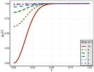
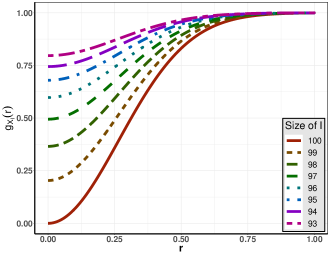
$d=10^{3}$, $\rho=500$	$d=10^{4}$, $\rho=500$

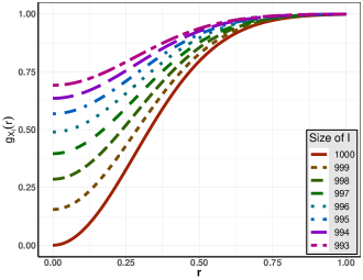
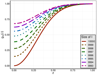
Figure 1: Pair correlation functions of the Gaussian DPP $\mathbf{X}$ (solid lines) with intensity $\rho_{\mathbf{X}}=500$ and $\alpha^{-1}=\rho_{\mathbf{X}}^{1/d}\sqrt{\pi}$ and its successive projections $\mathbf{X}_{I}$ ($\left|I\right|=d-1,\ldots$; dotted and dashed lines) for $d=10$ (top left), $10^{2}$ (top right), $10^{3}$ (bottom left) and $10^{4}$ (bottom right).

3.2 $L^{1}$-Exponential kernel

We now consider an exponential kernel, defined with respect to the $L^{1}$-norm instead of the Euclidean norm:

$$K(x-y)=\rho\exp\left(-\left\|\frac{x-y}{\alpha}\right\|_{1}\right).$$ (14)

The kernel (14) is referred to as the $L^{1}$-Exponential kernel in the following. It also constitutes a natural example as it satisfies ($H^{\prime\prime}$) where $K_{0}$ is defined for any $x,y\in\left[0{,}1\right]$ by:

$$K_{0}(x-y)=\rho^{1/d}\exp\left(-\left|\frac{x-y}{\alpha}\right|\right).$$

The existence of $\mathbf{X}\sim\mathrm{DPP}_{B}(K)$ is ensured if $\alpha$ is such that $\rho(2\alpha)^{d}\leq 1$. According to Theorem 2.1, for any $I\subseteq\overline{d}$, the pcf of $\mathbf{X}_{I}$ is given for any pairwise distinct $x,y\in B_{I}$ by

$$g_{\mathbf{X}_{I}}(x,y)=1-\kappa_{1}^{d-\iota}\exp\left(-2\left\|\frac{x-y}{\alpha}\right\|_{1}\right)$$ (15)

with

$$\kappa_{1}=\frac{\mathrm{tr}_{B_{0}}\left(K_{0}^{(2)}\right)}{\mathrm{tr}_{B_{0}}\left(K_{0}\right)^{2}}\approx\frac{\sum_{j\in\mathbb{Z}}\left(1+(2\pi\alpha j)^{2}\right)^{-2}}{\left(\sum_{j\in\mathbb{Z}}\left(1+(2\pi\alpha j)^{2}\right)^{-1}\right)^{2}}$$ (16)

where the approximation corresponds again to the Fourier approximation. For $d=10,10^{2},10^{3},10^{4}$, Figure 2 represents the pcfs of an $L^{1}$-Exponential DPP $\mathbf{X}$ (solid lines) and its successive projections with respect to the $L^{1}$-norm. The intensity parameter and $\alpha$ are set to $\rho_{\mathbf{X}}=500$ and $\alpha^{-1}=2\rho_{\mathbf{X}}^{1/d}$. The conclusion drawn from Figure 2 is similar to the one from Figure 1: the pcf of $\mathbf{X}_{I}$ is upper-bounded by 1, lower-bounded by $1-\kappa_{1}^{d-\iota}$ and tends to 1 when $\iota$ decreases. We could be tempted to compare Figures 1 and 2 and conclude that the Gaussian DPP seems more repulsive. However, remember that both models are not isotropic with respect to the same norm. We provide in Section 3.4 a summary statistic which allows us to correctly compare these models.

$d=10$, $\rho=500$	$d=100$, $\rho=500$
$d=10^{3}$, $\rho=500$	$d=10^{4}$, $\rho=500$

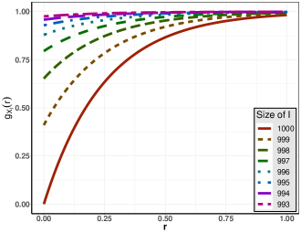
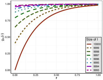
Figure 2: Pair correlation functions of the $L^{1}$-Exponential DPP $\mathbf{X}$ (solid lines) with intensity $\rho_{\mathbf{X}}=500$ and $\alpha^{-1}=2\rho_{\mathbf{X}}^{1/d}$ and its successive projections $\mathbf{X}_{I}$ ($\left|I\right|=d-1,\ldots$; dotted and dashed lines) for $d=10$ (top left), $10^{2}$ (top right), $10^{3}$ (bottom left) and $10^{4}$ (bottom right).

3.3 Dirichlet kernels

The two examples considered so far satisfy ($H^{\prime\prime}$) by definition. The next one is a projection kernel which only satisfies ($H^{\prime}$). For $\iota=1,\dots,d$, we let $\{\phi_{j}^{(\iota)}\}_{j\in\mathbb{Z}^{\iota}}$ denote the $\iota$-dimensional Fourier basis. We consider $d$ positive integers $(n_{i})_{i\in\overline{d}}$ and for $i\in\overline{d}$ the following one-dimensional stationary kernel:

$${K_{i}(x-y)=\sum_{j\in E_{i}}\phi^{(1)}_{j}(x-y)},{\color[rgb]{0,0,0}\quad x,y\in\left[0{,}1\right],}$$

where $E_{i}=\{a_{i},a_{i}+1,\dots,n_{i}-1+a_{i}\}$ is a set of $n_{i}$ consecutive integers and $a_{i}\in\mathbb{Z}$. Then, we construct a kernel $K$ as

$$K(x-y)=\prod_{i=1}^{d}K_{i}(x_{i}-y_{i})=\sum_{j\in E_{N}}\phi^{(d)}_{j}(x-y),{\color[rgb]{0,0,0}\quad x,y\in\left[0{,}1\right]^{d}}$$

where $E_{N}=\prod_{i}E_{i}$. It is worth pointing out that kernel $K$ can be written as

$$K(x-y)=\prod_{i=1}^{d}\left(\sum_{j=a_{i}}^{n_{i}-1+a_{i}}\phi_{j}^{(1)}(x_{i}-y_{i})\right)=\phi_{a}^{(d)}(y-x)\prod_{i=1}^{d}\left(\sum_{j=0}^{n_{i}-1}\phi_{j}^{(1)}(x_{i}-y_{i})\right)$$ (17)

where $a=(a_{i})_{i\in\overline{d}}$. Therefore, according to Remark (4) from [11, p. 48], the choice of the $E_{i}$’s does not influence the distribution of the DPP with kernel $K$. Remark that, if the $n_{i}$’s are all odd numbers and if we choose $a_{i}=-\lfloor n_{i}/2\rfloor$, the kernel $K$ equals

$$K(x-y)=\prod_{i=1}^{d}D_{\left\lfloor\frac{n_{i}}{2}\right\rfloor}(x_{i}-y_{i})$$ (18)

where $D_{p}$ is the Dirichlet kernel [[, e.g.]]Zygmund02 with parameter $p$. That terminology justifies the name Dirichlet kernel for this model. In the general case, and unambiguously we set $a_{i}=0$ for any $i$ and thus consider $E_{N}=\{j\in\mathbb{N}^{d}\,:\,j_{i}<n_{i},\,i=1\dots d\}$

$$K(x-y)=\sum_{j\in E_{N}}\mathrm{e}^{2\mathrm{i}\pi\left\langle j,x-y\right\rangle}.$$ (19)

A DPP on $B$ with kernel given by (19) is referred to as an $(N,d)$-Dirichlet kernel. From Theorem 2.1, for any $I\subseteq\overline{d}$, the pcf of $\mathbf{X}_{I}$ is given for any $x,y\in B_{I}$ by

$$g_{\mathbf{X}_{I}}(x,y) =1-\frac{1}{N}\sum_{j\in F_{N_{I}}}\left[\prod_{i\in I}\left(1-\frac{\left|j_{i}\right|}{n_{i}}\right)\right]\phi^{(\iota)}_{j}(x-y)$$

$$=1-\frac{1}{N}\prod_{i\in I}\sum_{|j|<n_{i}}\left(1-\frac{\left|j\right|}{n_{i}}\right)\phi^{(1)}_{j}(x_{i}-y_{i})$$ (20)

where $F_{N_{I}}=\{j\in\mathbb{Z}^{\iota}\,:\,\left|j_{i}\right|<n_{i},\,i\in I\}$. The pcf $g_{\mathbf{X}_{I}}$ is bounded from below by $1-\prod_{i\in I^{c}}n_{i}^{-1}$.

A question remains on the factorization of $N=\prod_{i=1}^{d}n_{i}$. We consider the factorization which minimizes the fluctuation of the $n_{i}$’s. For instance, when $N=100$ and $d=6$, we use $N=5\times 5\times 2\times 2\times 1\times 1$ while for $N=800$ we use the decomposition $N=5\times 5\times 4\times 2\times 2\times 2$.

The next section provides a summary statistics well-suited to the comparison of the three examples we have so far considered.

3.4 Normalized Ripley’s function

Since the Gaussian DPP and $L^{1}$-Exponential DPP are isotropic but with respect to a different norm and since the $(N,d)$-Dirichlet DPP is even not isotropic, it is hard to compare these different examples. In addition to the pcf, a way of characterizing regularity or repulsion in the literature is obtained by analyzing Ripley’s function [[, e.g.]]MollerWaagepeterson04. This function is not adapted for our framework. However, since all models satisfy ($H^{\prime}$), we propose to compare them through a normalized version of Ripley’s function based on the sup norm $\|\cdot\|_{\infty}$.

For a stationary spatial point process $\mathbf{X}$ on $B\subseteq\mathbb{R}^{d}$, we define the normalized $d$-dimensional Ripley’s function for some $r\geq 0$ by

$$R_{\mathbf{X}}(r)=\frac{\mathbb{E}\left(N_{\mathbf{X}}(B_{d,\infty}(0,r)\setminus 0)\mid 0\in\mathbf{X}\right)}{\mathbb{E}\left(N_{\mathbf{\Pi}}(B_{d,\infty}(0,r)\setminus 0)\mid 0\in\mathbf{\Pi}\right)}$$ (21)

where $B_{d,\infty}(0,r)=\{w\in\mathbb{R}^{d}:|w_{i}|\leq r,i=1,\dots,d\}$ is the $d$-dimensional ball with norm $\|\cdot\|_{\infty}$ centered at zero with radius $r$, $\mathbf{\Pi}$ is a homogeneous Poisson point process on $B$ with intensity $\rho$ and $N_{\mathbf{X}}(A)$ (resp. $N_{\mathbf{\Pi}}(A)$) denotes the number of points of $\mathbf{X}$ (resp. $\mathbf{\Pi}$) in a bounded subset $A\subset\mathbb{R}^{d}$. Assuming that $\mathbf{X}$ has a pcf, say $g_{\mathbf{X}}$, it is known from the properties of the second factorial moment that

$$R_{\mathbf{X}}(r)=\frac{\int_{B_{d,\infty}(0,r)}g_{\mathbf{X}}(w)\mathrm{d}w}{\int_{B_{d,\infty}(0,r)}g_{\mathbf{\Pi}}(w)\mathrm{d}w}=(2r)^{-d}\int_{B_{d,\infty}(0,r)}g_{\mathbf{X}}(w)\mathrm{d}w.$$ (22)

Obviously, under the Poisson case $R_{\mathbf{X}}=1$ whereas $R_{\mathbf{X}}<1$ means that $\mathbf{X}$ is repulsive. More precisely, the more $R_{\mathbf{X}}<1$ the more repulsive $\mathbf{X}$. We now present the interest of $R_{\mathbf{X}}$ in our context.

Proposition 3.1.

Let $\mathbf{X}\sim\mathrm{DPP}_{B}(K)$ be a DPP with kernel $K$ satisfying ($H^{\prime}$). Then, for any $I\subseteq\overline{d}$

$$R_{\mathbf{X}_{I}}(r)=1-\left(\prod_{i\in I^{c}}\frac{\mathrm{tr}_{B_{i}}\left(K_{i}^{(2)}\right)}{\mathrm{tr}_{B_{i}}\left(K_{i}\right)^{2}}\right)\left(\prod_{i\in I}\int_{0}^{1}\frac{\left|K_{i}(tr)\right|^{2}}{K_{i}(0)^{2}}\mathrm{d}t\right)$$ (23)

In particular, if $K$ satisfies ($H^{\prime\prime}$):

$$R_{\mathbf{X}_{I}}(r)=1-\kappa_{0}^{d-\iota}\left(\int_{0}^{1}\frac{\left|K_{0}(tr)^{2}\right|}{K_{0}(0)^{2}}\mathrm{d}t\right)^{\iota}$$ (24)

where

$$\kappa_{0}=\frac{\mathrm{tr}_{B_{0}}\left(K_{0}^{(2)}\right)}{\mathrm{tr}_{B_{0}}\left(K_{0}\right)^{2}}.$$

The proof of this result follows directly from (10) and (22). Focusing on examples presented in the previous sections, we have

$$R_{\mathbf{X}_{I}}(r)=\begin{cases}1-\kappa_{2}^{d-\iota}\left(\displaystyle\int_{0}^{1}\mathrm{e}^{-2t^{2}r^{2}/\alpha^{2}}\mathrm{d}t\right)^{\iota}&\text{for a Gaussian DPP,}\\[8.61108pt] 1-\kappa_{1}^{d-\iota}\left(\displaystyle\int_{0}^{1}\mathrm{e}^{-2tr/\alpha}\mathrm{\mathrm{d}}t\right)^{\iota}&\text{for an $L^{1}$-Exponential DPP,}\\[8.61108pt] 1-\dfrac{1}{N}\displaystyle\prod_{i\in I}\sum_{\left|j\right|<n_{i}}\left(1-\frac{\left|j\right|}{n_{i}}\right)\mathrm{sinc}(2\pi jr)&\text{for an $(N,d)$-Dirichlet DPP}\end{cases}$$

where $\kappa_{2}$ and $\kappa_{1}$ are defined by (13) and (16), respectively and $\mathrm{sinc}$ is the cardinal sine function.

Figures 3-5 investigate the situation for $d=6,10,100$ respectively. Ripley’s functions for point processes $\mathbf{X}_{I}$ based on the three models exposed in this section are depicted. The intensity is set to $\rho_{\mathbf{X}}=500$ and $\iota=d-i$ for $i=0,\dots,5$. The Gaussian DPP and $L^{1}$-Exponential DPP satisfy ($H^{\prime\prime}$), and so we decide, without loss of generality, to discard the last coordinates to define the projections. Since the $(N,d)$-Dirichlet DPP satisfies only ($H^{\prime}$), the choice of directions has an influence. For this process, Ripley’s functions have been computed using a Monte-Carlo approach (based on $10^{4}$ replications): the coordinates to be removed are randomly chosen. The plots for the $(N,d)$-Dirichlet DPPs represent therefore the empirical mean of Ripley’s functions. First and third quartiles are also represented by envelops to get an idea of the variability. The visual results show that for $\rho_{\mathbf{X}}=500$, the $(N,d)$-Dirichlet DPP is the most repulsive among the three models. Moreover, the loss of repulsiveness when projecting turns out to be smaller for $(N,d)$-Dirichlet DPPs than for the two other DPP models. The envelops reported for the $(N,d)$-Dirichlet should be taken with attention. We could be tempted to conclude that the quite high variability observed for $d=6,10$, is too important to get practical interesting results. However, Section 4 will discredit this argument.

The $(N,d)$-Dirichlet DPP is the most repulsive in the situations considered here. However, it is worth mentioning that it may behave very badly according to the value of $N$. For example, we have observed that the less $N$ has factors the less repulsive the $(N,d)$-Dirichlet DPP. The values of these factors also affect the repulsiveness of the DPP. In particular, if $N$ is a high prime number, both situations are encountered which yields a disastrous model in terms of repulsion. Figures 3-5 underline that the class of $L^{1}$-Exponential DPP is definitely less interesting than the class of Gaussian DPP. Given an $\iota$, Ripley’s function is closer to 1 and the convergence to 1 when $\iota$ decreases is faster for $L^{1}$-Exponential DPP. For this reason, the $L^{1}$-Exponential DPP is not considered in the next section.

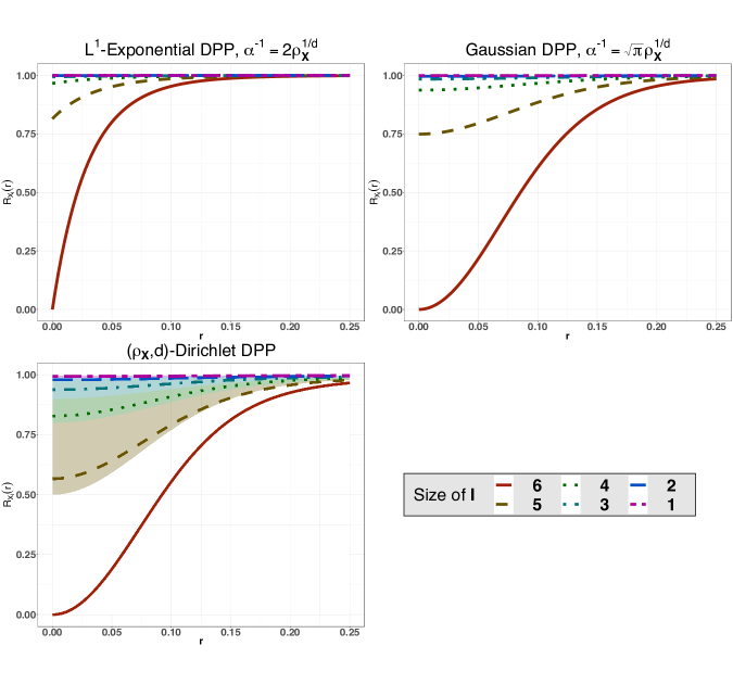
Figure 3: Ripley’s functions (see (22)) of a $6$-dimensional DPP $\mathbf{X}$ with intensity $\rho_{\mathbf{X}}$ (solid lines) and its successive projections $\mathbf{X}_{I}$ ($\left|I\right|=d-1,\ldots$; dotted and dashed lines) for the $L^{1}$-Exponential DPP (top-left), Gaussian DPP (top right) and the $(N,6)$-Dirichlet DPP (bottom left). For the Dirichlet case, coordinates to be removed are chosen randomly ($10^{4}$ replications): dotted and dashed lines represent empirical means while first and third quartiles are represented by envelops.

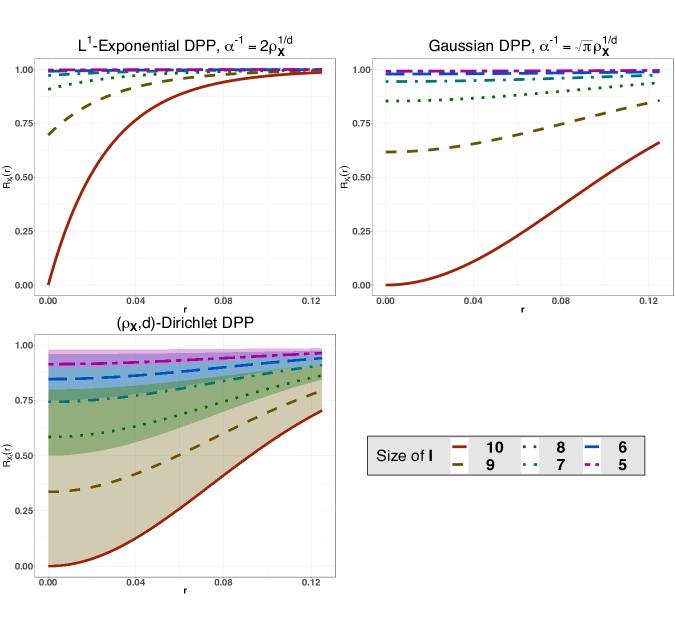
Figure 4: Ripley’s functions (see (22)) of a $10$-dimensional DPP $\mathbf{X}$ with intensity $\rho_{\mathbf{X}}$ (solid lines) and its successive projections $\mathbf{X}_{I}$ ($\left|I\right|=d-1,\ldots$; dotted and dashed lines) for the $L^{1}$-Exponential DPP (top-left), Gaussian DPP (top right) and the $(N,10)$-Dirichlet DPP (bottom left). For the Dirichlet case, coordinates to be removed are chosen randomly ($10^{4}$ replications): dotted and dashed lines represent empirical means while first and third quartiles are represented by envelops.

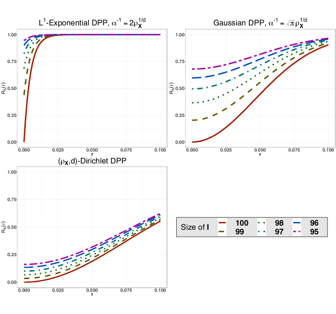
Figure 5: Ripley’s functions (see (22)) of a $100$-dimensional DPP $\mathbf{X}$ with intensity $\rho_{\mathbf{X}}$ (solid lines) and its successive projections $\mathbf{X}_{I}$ ($\left|I\right|=d-1,\ldots$; dotted and dashed lines) for the $L^{1}$-Exponential DPP (top-left), Gaussian DPP (top right) and the $(N,100)$-Dirichlet DPP (bottom left). For the Dirichlet case, coordinates to be removed are chosen randomly ($10^{4}$ replications): dotted and dashed lines represent empirical means while first and third quartiles are represented by envelops.

4 Numerical illustrations

In this section, we illustrate the interest of projected DPP models by simulation experiments. For some $d\geq 1$ and $I\subseteq\overline{d}$, the problem we consider is to estimate using a Monte-Carlo approach, an integral of the form

$$\mu(f_{I})=\int_{{\color[rgb]{0,0,0}\left[0{,}1\right]^{d}}}f_{I}(u)\mathrm{d}u$$

where $f_{I}:{\color[rgb]{0,0,0}\left[0{,}1\right]^{\iota}}\to\mathbb{R}^{+}$ is a $\iota$-dimensional function. A standard way for achieving this task (which includes the uniform sampling design) is to define a point process, say $\mathbf{Z}_{I}$, on ${\color[rgb]{0,0,0}\left[0{,}1\right]^{\iota}}$ and estimate $\mu(f_{I})$ using the unbiased estimator

$$\widehat{\mu}_{\mathbf{Z}_{I}}(f_{I})=\rho_{\mathbf{Z}_{I}}^{-1}\sum_{u\in\mathbf{Z}_{I}}f_{I}(u).$$ (25)

Given $I$ and $f_{I}$, this problem has been widely considered in the literature [[, e.g.]]RobertCasella04, DelyonPortier16. In particular, an ad-hoc DPP on ${\color[rgb]{0,0,0}\left[0{,}1\right]^{\iota}}$, for which very interesting asymptotic results have been shown, has been proposed in [2]. In this section, we investigate another aspect. We consider the problem not only for one but various integrals, defined for different subsets $I\subseteq\overline{d}$ and based on a single realization of a point process defined on $\left[0{,}1\right]^{d}$. This problem, for which investigated models are definitely meaningful, mimics problems encountered in computer experiments where the spatial design is initially defined on $\mathbb{R}^{d}$ but later used with a few coordinates discarded [[, e.g.]]WoodsLewis16, Kleijnen17.

To do this, we therefore consider a spatial point process $\mathbf{X}$ (and in particular DPP models developed in the previous section) and we estimate $\mu(f_{I})$ by (25) with $\mathbf{Z}_{I}=\mathbf{X}_{I}$ where $\mathbf{X}_{I}$ is the projected point pattern of $\mathbf{X}$ on ${\color[rgb]{0,0,0}\left[0{,}1\right]^{\iota}}$. The interest of our models lies in the following equation which evaluates $\mathrm{Var}(\widehat{\mu}_{\mathbf{X}_{I}}(f_{I}))$. Using Campbell Theorem (1)

$$\mathrm{Var}\left(\widehat{\mu}_{\mathbf{X}_{I}}(f_{I})\right) =\rho_{\mathbf{X}_{I}}^{-1}\int_{{\color[rgb]{0,0,0}\left[0{,}1\right]^{\iota}}}f_{I}(u)^{2}\mathrm{d}u$$ (26)

$$\quad+\int_{{\color[rgb]{0,0,0}\left[0{,}1\right]^{\iota}}}\int_{{\color[rgb]{0,0,0}\left[0{,}1\right]^{\iota}}}(g_{\mathbf{X}_{I}}(u,v)-1)f_{I}(u)f_{I}(v)\mathrm{d}u\mathrm{d}v.$$

As soon as $g_{\mathbf{X}_{I}}<1$, the variance is smaller than the first integral which turns out to be the variance under the Poisson case. In this section, we intend to verify this property with models considered in this paper.

In the following, we let $d=6$ and, following [2, Sec. 3], we consider for any $I\subseteq\overline{6}$ the “bump” test function

$$f_{I}(u)=\exp\left(-\sum_{i\in I}{\color[rgb]{0,0,0}\frac{1}{1-4(u_{i}-1/2)^{2}}}\right),\quad u\in{\color[rgb]{0,0,0}\left[0{,}1\right]^{\iota}}.$$ (27)

Three type of models are investigated: a homogeneous Poisson point process (which serves as a reference), a Gaussian DPP, and an $(N,6)$-Dirichlet DPP. Simulations of DPPs can be realized using R package spatstat. However, using this package leads to performance issues (in particular in terms of memory) when simulating DPPs with high intensity and/or high dimension. Therefore, we have implemented the simulation algorithms in C++ and have made them usable with R. The codes are available on GitHub (https://github.com/AdriMaz/rcdpp/).

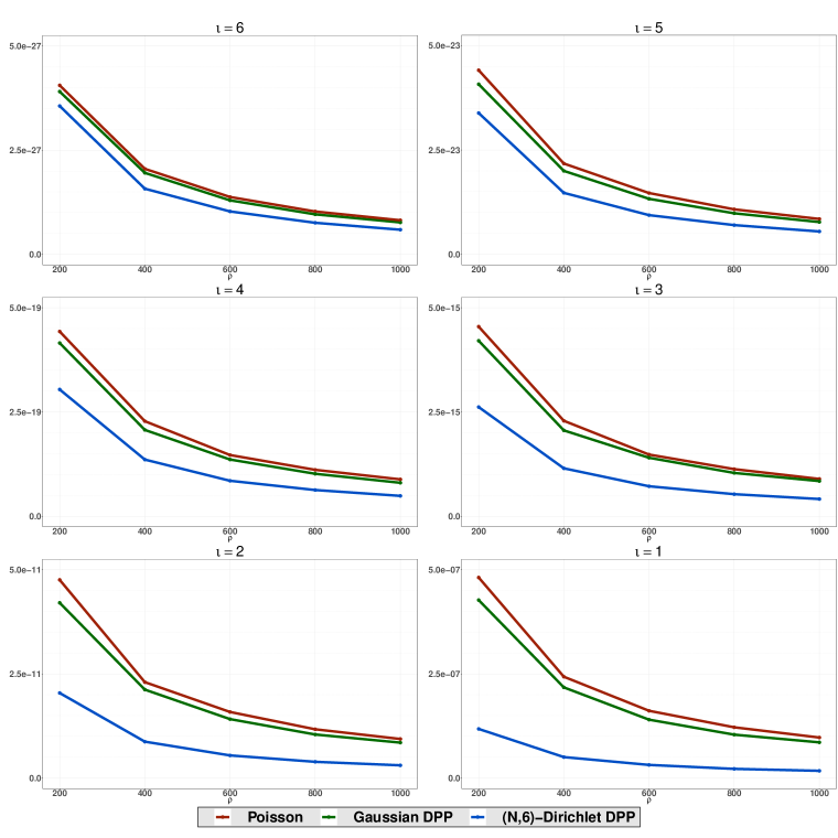
Figure 6: Empirical variances of Monte-Carlo integral estimates of the form (25) for the function (27) using Poisson process (red lines), Gaussian DPP (green lines) and Dirichlet DPP (blue lines) for $\iota=\left|I\right|=6,\ldots,1$, based on $10^{4}$ replications of a $6$-dimensional point processes with intensity $\rho_{\mathbf{X}}=200,400,600,800,1000$. When $\iota<6$, coordinates to be removed are chosen randomly.

Figure 6 reports empirical variances of estimates of $\mu(f_{I})$ based on $m=10^{4}$ replications of each model, in terms of $\rho_{\mathbf{X}}$ where $\rho_{\mathbf{X}}=200,400,600,800,1000$. We consider all possible projections, i.e. $\iota=6,5,4,3,2,1$. For the Poisson case, note that $\mathbf{X}_{I}$ has the same distribution as a homogeneous Poisson point process (with the same intensity) defined on $B_{I}$. For the Gaussian DPP, the parameter $\alpha$ is set to $\alpha^{-1}=\sqrt{\pi}\rho^{1/6}$. When $\iota<d$, the coordinates to be discarded are chosen randomly. This has no influence for the Poisson, Gaussian DPP since these models satisfy Assumption ($H^{\prime\prime}$) but is important for the $(N,6)$-Dirichlet DPP.

Figure 6 illustrates the interest of this research. It is clear that whatever the dimension of the function to integrate, i.e. whatever $\iota=6,\dots,1$, the empirical variance of Monte-Carlo estimates using one single realization of a spatial point process defined in dimension $d$, is always smaller than in the independent case. The $(N,d)$-Dirichlet model outperforms the Gaussian DPP for any $I\subseteq\overline{d}$ as already observed from a theoretical point of view in the previous section. The general result of this paper states that a projected DPP seems less and less repulsive after successive projections. However, It is interesting to observe that this fact does not affect that much the properties of Monte-Carlo integration estimates.

Conclusion

The objective of this paper is to explore properties of projections of a DPP $\mathbf{X}$ with kernel $K$ and defined on a compact set $B$ of $\mathbb{R}^{d}$. For any $I\subset\{1,\dots,d\}$, our general conclusion is that the projection $\mathbf{X}_{I}$ remains repulsive when kernel $K$ is separable, in the sense that $g_{\mathbf{X}_{I}}<1$ uniformly for any $I\subset\{1,\dots,d\}$. In particular if kernel $K$ is a projection kernel, $\mathbf{X}_{I}$ falls in the class of $\alpha$-DPPs (with $\alpha=-1/n,n\in\mathbb{N}$). We have proposed a few examples of such separable kernels and compared them using an original summary statistic based on a normalized version of the Ripley’s function defined with the sup norm. We have finally illustrated this paper for Monte-Carlo integration problems when the problem is to estimate integrals over a compact set $B_{I}$ of an $\iota$-dimensional function for any $1\leq\iota\leq d$, using the same quadrature points defined in $B$. To be fully relevant, comparisons with designs built from other classes of point processes (e.g. Gibbs, Matérn, Multivariate OP Ensembles), more standard designs (e.g. Halton, Sobol, Quasi-Monte-Carlo), in which other test functions with different properties (e.g. less regular or non-compactly supported) would be considered, should be performed. We leave this for a future research.

Appendix A Proof of Lemma 2.1

Proof.

For any non-negative measurable function $h_{I}:B_{I}^{k}\to\mathbb{R}^{+}$, we have using Campbell Theorem (1)

$$\int_{B_{I}^{k}} h_{I}\left(x_{I}^{(1)},\ldots,x_{I}^{(k)}\right)\rho_{\mathbf{X}_{I}}^{(k)}\left(x_{I}^{(1)},\ldots,x_{I}^{(k)}\right)\mathrm{d}x_{I}^{(1)}\ldots\mathrm{d}x_{I}^{(k)}$$

$$=\mathbb{E}\left[\sum_{x_{I}^{(1)},\ldots,x_{I}^{(k)}\in\mathbf{X}_{I}}^{\neq}h_{I}\left(x_{I}^{(1)},\ldots,x_{I}^{(k)}\right)\right]$$

$$=\mathbb{E}\left[\sum_{x^{(1)},\ldots,x^{(k)}\in\mathbf{X}}^{\neq}(h_{I}\circ P_{I})\left(x^{(1)},\ldots,x^{(k)}\right)\right]$$

$$=\int_{B_{I}^{k}}h_{I}\left(x_{I}^{(1)},\ldots,x_{I}^{(k)}\right)\bigg{\{}\int_{(B_{I^{c}})^{k}}\rho_{\mathbf{X}}^{(k)}\left(\left(x^{(1)},u^{(1)}\right),\ldots,\left(x^{(k)},u^{(k)}\right)\right)$$

$$\qquad\qquad\mathrm{d}u^{(1)}\ldots\mathrm{d}u^{(k)}\bigg{\}}\mathrm{d}x_{I}^{(1)}\ldots\mathrm{d}x_{I}^{(k)}$$

whereby we deduce (2.1) by identification. ∎

Appendix B Proof of Theorem 2.1

Proof.

Let us write (8) under ($H[I]$).

$$\rho_{\mathbf{X}_{I}}^{(k)}\left(x^{(1)},\ldots,x^{(k)}\right) =\sum_{\sigma\in S_{k}}(-1)^{k-C(\sigma)}\int_{(B_{I^{c}})^{k}}\prod_{i=1}^{k}K\left((x,u)^{(i)},(x,u)^{(\sigma(i))}\right)\mathrm{d}u^{(1)}\ldots\mathrm{d}u^{(k)}$$

$$=\sum_{\sigma\in S_{k}}(-1)^{k-C(\sigma)}\prod_{i=1}^{k}K_{I}\left(x_{I}^{(i)},x_{I}^{(\sigma(i))}\right)$$

$$\phantom{\sum_{\sigma\in S_{k}}\qquad}\times\int_{(B_{I^{c}})^{k}}\prod_{i=1}^{k}K_{I^{c}}(u^{(i)},u^{(\sigma(i))})\mathrm{d}u^{(1)}\ldots\mathrm{d}u^{(k)}.$$ (28)

For any $\sigma\in S_{k}$ let us denote by $\mathrm{supp}(\sigma)$ its support:

$$\mathrm{supp}(\sigma)=\{i\in\overline{k}\mbox{ s.t. }\sigma(i)\neq i\},$$

by $c(\sigma)$ the number of elements of $\mathrm{supp}(\sigma)$, by $\mathcal{S}(\sigma)$ the set of disjoint cycles of $\sigma$ with non-empty support and by $C(\sigma)$ the number of disjoint cycles of $\sigma$ (including those with empty support). Consider the case where $C(\sigma)=1$ (i.e. $\sigma$ is a circular permutation of $\overline{k}$). Then the integral part in (B) can be written as

$$\int_{(B_{I^{c}})^{k}}\prod_{i=1}^{k}K_{I^{c}}\left(u^{(i)},u^{(\sigma(i))}\right)\mathrm{d}u^{(1)}\ldots\mathrm{d}u^{(k)}$$

$$=\int_{(B_{I^{c}})^{k}}K_{I^{c}}\left(u^{(1)},u^{(\sigma(1))}\right)\ldots K_{I^{c}}\left(u^{(\sigma(1))},u^{(\sigma^{2}(1))}\right)\ldots$$

$$\qquad\dots K_{I^{c}}\left(u^{(k)},u^{(\sigma(k))}\right)\mathrm{d}u^{(1)}\ldots\mathrm{d}u^{(\sigma(1))}\ldots\mathrm{d}u^{(k)}$$

$$=\int_{(B_{I^{c}})^{k-1}}K_{I^{c}}^{(2)}\left(u^{(1)},u^{(\sigma^{2}(1))}\right)\ldots$$

$$\phantom{\int_{(B_{I^{c}})^{k}}}\ldots K_{I^{c}}\left(u^{(\sigma(1)-1)},u^{(\sigma(\sigma(1)-1))}\right)K_{I^{c}}\left(u^{(\sigma(1)+1)},u^{(\sigma(\sigma(1)+1))}\right)\ldots$$

$$\phantom{\int_{(B_{I^{c}})^{k}}}\ldots K_{I^{c}}\left(u^{(k)},u^{(\sigma(k))}\right)\mathrm{d}u^{(1)}\ldots\mathrm{d}u^{(\sigma(1)-1)}\mathrm{d}u^{(\sigma(1)+1)}\ldots\mathrm{d}u^{(k)}$$

$$\vdots$$

$$=\int_{(B_{I^{c}})^{2}}K_{I^{c}}^{(k-1)}\left(u^{(1)},u^{(\sigma^{k-1}(1))}\right)K_{I^{c}}\left(u^{(\sigma^{k-1}(1))},u^{(\sigma^{k}(1))}\right)\mathrm{d}u^{(1)}\mathrm{d}u^{(\sigma^{k-1}(1))}$$

$$=\mathrm{tr}_{B_{I^{c}}}\left(K_{I^{c}}^{(k)}\right).$$

Assume now that $C(\sigma)>1$. Then $\sigma$ can be written as

$$\sigma=\left(\bigodot_{\varepsilon\in\mathcal{S}(\sigma)}\varepsilon\right)\odot\mathbf{i}_{k}(\sigma),$$ (29)

where $\mathbf{i}_{k}(\sigma)$ is the identity on $\overline{k}\setminus\mathrm{supp}(\sigma)$, and $\odot$ denotes the permutation product. Observe that (29) implies

$$C(\sigma)=\#S(\sigma)+k-c(\sigma).$$ (30)

If $1\in\mathrm{supp}(\sigma)$, there is only one permutation $\varsigma\in\mathcal{S}(\sigma)$ such that $1\in\mathrm{supp}(\varsigma)$. Therefore:

$$\int_{(B_{I^{c}})^{k}}\prod_{i=1}^{k}K_{I^{c}}\left(u^{(i)},u^{(\sigma(i))}\right)\mathrm{d}u^{(1)}\ldots\mathrm{d}u^{(k)}$$

$$=\mathrm{tr}_{B_{I^{c}}}\left(K^{(c(\iota))}\right)\int_{(B_{I^{c}})^{k-c(\varsigma)}}\prod_{i\in\overline{k}\setminus\mathrm{supp}(\varsigma)}K_{I^{c}}\left(u^{(i)},u^{(\sigma(i))}\right)\mathrm{d}u^{(1)}\ldots\mathrm{d}u^{(k)}$$

Denote by $\alpha$ the minimum of $\overline{k}\setminus\mathrm{supp}(\varsigma)$. As above there is only one permutation $\varsigma^{\prime}\in\mathcal{S}(\sigma)$ such that $\alpha\in\mathrm{supp}(\varsigma^{\prime})$. Then:

$$\int_{(B_{I^{c}})^{k}}\prod_{i=1}^{k}K_{I^{c}}\left(u^{(i)},u^{(\sigma(i))}\right)\mathrm{d}u^{(1)}\ldots\mathrm{d}u^{(k)}$$

$$=\mathrm{tr}_{B_{I^{c}}}\left(K_{I^{c}}^{(c(\varsigma))}\right)\int_{(B_{I^{c}})^{k-c(\varsigma)}}\prod_{i\in\overline{k}\setminus\mathrm{supp}(\varsigma)}K_{j}\left(u^{(i)},u^{(\sigma(i))}\right)\mathrm{d}u^{(1)}\ldots\mathrm{d}u^{(k)}$$

$$=\mathrm{tr}_{B_{I^{c}}}\left(K_{I^{c}}^{(c(\varsigma))}\right)\mathrm{tr}_{B_{j}}\left(K_{I^{c}}^{(c(\varsigma^{\prime}))}\right)$$

$$\;\times\int_{(B_{I^{c}})^{k-(c(\varsigma)+c(\varsigma^{\prime})}}\prod_{i\in\overline{k}\setminus\left(\mathrm{supp}(\varsigma)\cup\mathrm{supp}(\varsigma^{\prime})\right)}K_{I^{c}}\left(u^{(i)},u^{(\sigma(i))}\right)\mathrm{d}u^{(1)}\ldots\mathrm{d}u^{(k)}.$$

Therefore, one gets by induction:

$$\int_{(B_{I^{c}})^{k}}\prod_{i=1}^{k}K_{I^{c}}\left(u^{(i)},u^{(\sigma(i))}\right)\mathrm{d}u^{(1)}\ldots\mathrm{d}u^{(k)}$$

$$=\left[\prod_{\varepsilon\in\mathcal{S}(\sigma)}\mathrm{tr}_{B_{I^{c}}}\left(K_{I^{c}}^{(c(\varepsilon))}\right)\right]\int_{(B_{I^{c}})^{k-c(\sigma)}}\prod_{i\in\overline{k}\setminus\mathrm{supp}(\sigma)}K_{I^{c}}\left(u^{(i)},u^{(\sigma(i))}\right)\mathrm{d}u^{(1)}\ldots\mathrm{d}u^{(k)}.$$ (31)

Plugging (B) into (B) leads to (9).

∎

Appendix C Laplace functionals

Lemma C.1.

Let $I\subset\overline{d}$ and let $\mathbf{X}$ be a spatial point process defined on a compact set $B\subset\mathbb{R}^{d}$. Then, for any Borel function $h_{I}:B_{I}\rightarrow\mathbb{R}^{+}$

$$\mathcal{L}_{\mathbf{X}_{I}}(h_{I})=\mathcal{L}_{\mathbf{X}}(h_{I}\circ P_{I}).$$ (32)

Proof.

Equation (32) follows arguments similar to the ones used in the proof of Lemma 2.1.

$$\mathcal{L}_{\mathbf{X}_{I}}(h_{I})=\mathbb{E}\left[\prod_{y\in\mathbf{X}_{I}}\mathrm{e}^{-h_{I}(y)}\right]=\mathbb{E}\left[\prod_{x\in\mathbf{X}}\mathrm{e}^{-h_{I}(x_{I})}\right]=\mathcal{L}_{\mathbf{X}}(h_{I}\circ P_{I})$$

∎

Theorem C.1.

Let $I\subseteq\overline{d}$ and $\mathbf{X}\sim\mathrm{DPP}_{B}(K)$ such that $K$ satisfies ($H[I]$). The Laplace functional of the projected point process $\mathbf{X}_{I}$ is given for any Borel function $h_{I}:B_{I}\rightarrow\mathbb{R}^{+}$ by:

$$\mathcal{L}_{\mathbf{X}_{I}}(h_{I}) =\prod_{l\in\mathcal{N}_{I^{c}}}\exp\left\{-\sum_{k\geq 1}\frac{\mathrm{tr}_{B_{I}}\left({K}_{\lambda_{l}^{(I^{c})}K_{I},h_{I}}^{(k)}\right)}{k}\right\}$$ (33)

$$=\exp\left\{-\sum_{k\geq 1}\frac{\mathrm{tr}_{B_{I^{c}}}\left(K_{I^{c}}^{(k)}\right)\mathrm{tr}_{B_{I}}\left({K}_{I,h_{I}}^{(k)}\right)}{k}\right\}$$ (34)

where $K_{I,h_{I}}:B_{I}\times B_{I}\rightarrow\mathbb{C}$ is the kernel defined by

$$K_{I,h_{I}}(x,y)=\sqrt{1-\mathrm{e}^{-h_{I}(x)}}K_{I}(x,y)\sqrt{1-\mathrm{e}^{-h_{I}(y)}}.$$

Proof.

The proof is straightforward and follows from Lemma C.1, assumption ($H[I]$) and the definition of $K_{I,h_{I}}$. ∎

References

- [1] A. Baddeley “Spatial Point Processes and their Applications” In Stochastic geometry: Lectures given the C.I.M.E. Summer School held in Martina Franca, Italy, September 13–18, 2004 Berlin, Heidelberg: Springer, 2007, pp. 1–75
- [2] R. Bardenet and A. Hardy “Monte Carlo with determinantal point processes” (to appear) In Ann. Appl. Probab., 2020
- [3] L. Debnath and P. Mikusiński “Introduction to Hilbert spaces with applications” Elsevier Academic Press, 2005
- [4] L. Decreusefond, I. Flint, N. Privault and G.L. Torris “Determinantal point processes” In Stochastic Analysis for Poisson Point Processes Cham: Springer International Publishing, 2016, pp. 311–342
- [5] B. Delyon and F. Portier “Integral approximation by kernel smoothing” In Bernoulli 22.4, 2016, pp. 2177–2208
- [6] D. Dereudre “Introduction to the theory of Gibbs point processes” In Stochastic Geometry Springer, 2019, pp. 181–229
- [7] D. Dupuy, C. Helbert and J. Franco “DiceDesign and DiceEval: Two R Packages for Design and Analysis of Computer Experiments” In J. Stat. Softw. 65.11, 2015, pp. 1–38
- [8] J. Franco, X. Bay, D. Dupuy and B. Corre “Planification d’expériences numériques à partir du processus ponctuel de Strauss” working paper or preprint, 2008 URL: https://hal.archives-ouvertes.fr/hal-00260701
- [9] J. H. Halton “Algorithm 247: Radical-inverse Quasi-random Point Sequence” In Communications ACM 7.12, 1964, pp. 701–702
- [10] J.B. Hough, M. Krishnapur, Y. Peres and B. Virág “Determinantal Processes and Independence” In Probability Surveys 3, 2006, pp. 206–229
- [11] J.B. Hough, M. Krishnapur, Y. Peres and B. Virág “Zeros of Gaussian Analytic Functions and Determinantal Point Processes” American Mathematical Society, 2009
- [12] J. Illian, A. Penttinen, H. Stoyan and D. Stoyan “Statistical Analysis and Modelling of Spatial Point Patterns.”, Statistics in Practice Chichester: Wiley, 2008
- [13] J.P. Kleijnen “Design and analysis of simulation experiments: tutorial” In Advances in Modeling and Simulation New York: Springer, 2017, pp. 135–158
- [14] F. Lavancier, J. Møller and E. Rubak “Determinantal point process models and statistical inference: Extended version” In J. Roy. Stat. Soc. B 77.4, 2015, pp. 853–877
- [15] O. Macchi “The coincidence approach to stochastic processes” In Adv. Appl. Probab. 7, 1975, pp. 83–122
- [16] P. McCullagh and J. Møller “The permanental process” In Adv. Appl. Prob. 38, 2006, pp. 873–88
- [17] M.D. McKay, R. J. Beckman and W.J. Conover “A comparison of three methods for selecting values of input variables in the analysis of output from a computer code” In Technometrics 21, 1979, pp. 239–245
- [18] J. Møller and R.P. Waagepetersen “Statistical Inference and Simulation for Spatial Point Processes” Boca Raton: ChapmanHall/CRC, 2004
- [19] A.B. Owen “Monte Carlo theory, methods and examples”, 2013
- [20] A.B. Owen “Orthogonal arrays for computer experiments, integration and visualization” In Stat. Sinica 2, 1992, pp. 439–452
- [21] F. Riesz and B. Sz-Nagy “Functional Analysis” New York: Dover Publications, 1990
- [22] C.P. Robert and G. Casella “Monte Carlo Statistical Methods” New York: Springer-Verlag, 2004
- [23] T.J. Santner, B.J. Williams and W.I. Notz “The design and analysis of computer experiments” Springer Science & Business Media, 2013
- [24] T. Shirai and Y. Takahashi “Random point fields associated with certain Fredholm determinants I. Fermion, Poisson and boson point processes” In J. Funct. Anal. 205, 2003, pp. 414–463
- [25] I.M. Sobol “On the distribution of points in a cube and the approximate evaluation of integrals” In USSR Comp. Math. Math+ 7.4, 1967, pp. 86 –112
- [26] A. Soshnikov “Determinantal random point fields” In Russ. Math. Surv+ 55.5, 2000, pp. 923–975
- [27] F. Sun, Y. Wang and H. Xu “Uniform projection designs” In Ann. Stat. 47.1, 2019, pp. 641–661
- [28] J. Teichmann, F. Ballani and K.G. Boogaart “Generalizations of Matérn’s hard-core point processes” In Spat. Stat.-Neth. 3, 2013, pp. 33–53
- [29] D.C Woods and S.M. Lewis “Design of experiments for screening” In Handbook of Uncertainty Quantification New York: Springer, 2006, pp. 1143–1185
- [30] A. Zygmund “Trigonometric Series (Volumes I & II combined)” Cambridge University Press, 2003