Impact of magnetic nanoparticles on the Casimir pressure in three-layer systems

Abstract

The Casimir pressure is investigated in three-layer systems where the intervening stratum possesses magnetic properties. This subject is gaining in importance in connection with ferrofluids and their use in various microelectromechanical devices. We present general formalism of the Lifshitz theory adapted to the case of ferrofluid sandwiched between two dielectric walls. The Casimir pressure is computed for the cases of kerosene- and water-based ferrofluids containing a 5$\%$ fraction of magnetite nanoparticles with different diameters between silica glass walls. For this purpose, we have found the dielectric permittivities of magnetite and kerosene along the imaginary frequency axis employing the available optical data and used the familiar dielectric properties of silica glass and water, as well as the magnetic properties of magnetite. We have also computed the relative difference in the magnitudes of the Casimir pressure which arises on addition of magnetite nanoparticles to pure carrier liquids. It is shown that for nanoparticles of 20 nm diameter at 2 micrometer separation between the walls this relative difference exceeds 140$\%$ and 25$\%$ for kerosene- and water-based ferrofluids, respectively. An interesting effect is found that at a fixed separation between the walls an addition of magnetite nanoparticles with some definite diameter makes no impact on the Casimir pressure. The physical explanation for this effect is provided. Possible applications of the obtained results are discussed.

I Introduction

It has long been known that with decreasing distance between two adjacent surfaces the van der Waals b1 and Casimir b2 forces come into play which are caused by the zero-point and thermal fluctuations of the electromagnetic field. These forces are of common nature. In fact, the van der Waals force is a special case of the Casimir force when the separation distance reduces to below a few nanometers, where the effects of relativistic retardation are negligibly small. The theory of the van der Waals and Casimir forces was developed by E. M. Lifshitz and his collaborators b3 ; b4 . In the framework of this theory, the force value is expressed via the frequency-dependent dielectric permittivities and magnetic permeabilities of the boundary surfaces. For ordinary, nonmagnetic, surfaces the Casimir force through a vacuum gap is always attractive. If, however, the gap is filled with a liquid, the Casimir force may be repulsive if the dielectric permittivities of the boundary surfaces and of a liquid satisfy some condition b3 ; b4 . This is the case of a three-layer system which suggests a wide variety of different options.

By now many measurements of the Casimir force acting through a vacuum gap have been performed between both nonmagnetic (see Refs. b2 ; b5 ; b6 for a review) and magnetic b7 ; b8 ; b9 ; b10 materials. The attractive and repulsive forces in the three-layer systems involving a liquid stratum were measured as well b11 ; b12 ; b13 . The obtained results have been used to devise various micro- and nanodevices actuated by the Casimir force b14 ; b15 ; b16 ; b17 ; b18 ; b19 ; b20 ; b21 ; b22 ; b23 ; b24 . All of them, however, exploit the Casimir force through a vacuum gap for their functionality. At the same time, the so-called magnetic (or ferro) fluids b25 , which consist of some carrier liquid and the magnetic nanoparticles coated with a surfactant to prevent their agglomeration, find expanding applications in the mechanical engineering, electronic devices, optical modulators and switchers, optoelectronic communications, biosensors, medical technologies etc. (see Ref. b26 for a review and, e.g., Refs. b27 ; b28 ; b29 ; b30 ). Among them, from the viewpoint of Casimir effect, the applications of greatest interest are to micromechanical sensors b31 , microfluidics b32 ; b33 and microrobotics b34 , where ferrofluids may be confined between two closely spaced surfaces, forming the three-layer system. Note, however, that the Casimir force in systems of this kind, having a magnetic intervening stratum, was not investigated so far.

In this paper, we consider an impact of magnetic nanoparticles on the Casimir pressure in three-layer systems, where the magnetic fluid is confined in between two glass plates. The cases of kerosene- and water-based ferrofluids are treated which form a colloidal suspension with magnetite nanoparticles of some diameter $d$. The Casimir pressure in the three-layer systems with a magnetic intervening stratum is calculated in the framework of the Lifshitz theory b2 ; b3 ; b4 . For this purpose, we find the dielectric permittivity of kerosene and both the dielectric and magnetic characteristics of magnetite and ferrofluids at the pure imaginary Matsubara frequencies.

The computational results are presented for both the magnitude of the Casimir pressure through a ferrofluid and for the impact of magnetic nanoparticles on the Casimir pressure through a nonmagnetic fluid. These results are shown as function of separation distance between the plates and of a nanoparticle diameter. The effect of the conductivity of magnetite at low frequencies on the results obtained is discussed. We show that the presence of magnetic nanoparticles in the intervening liquid makes a significant impact on the magnitude of the Casimir pressure. Thus, for the $5\%$ fraction of magnetic nanoparticles with 20 nm diameter in a kerosene-based ferrofluid, at $2~{}\mu$m separation between the walls, this impact exceeds $140\%$. For a water-based ferrofluid under the same conditions the presence of magnetic nanoparticles enhances the magnitude of the Casimir pressure by $25\%$. Another important result is that at a fixed separation the presence of magnetic nanoparticles of some definite diameter makes no impact on the Casimir pressure. The physical reasons for this conclusion are elucidated.

The paper organized as follows. In Sec. II, we present the formalism of the Lifschitz theory adapted for a three-layer system with magnetic intervening stratum. We also find the dielectric permittivity and magnetic permeability of magnetite along the imaginary frequency axis and include necessary information regarding the dielectric permittivity of a colloidal suspension. Section III contains evaluation of the dielectric permittivity of kerosene and kerosene-based ferrofluids along the imaginary frequency axis. Here we calculate the Casimir pressure in such ferrofluids and investigate the role of magnetite nanoparticles in the obtained results. In Sec. IV the same is done for the case of water-based ferrofluids. In Sec. V the reader will find our conclusions and a discussion.

II General formalism for three-layer systems with
magnetite nanoparticles

We consider the three-layer system consisting of two parallel nonmagnetic dielectric walls described by the frequency-dependent dielectric permittivity $\varepsilon(\omega)$ and separated by the gap of width $a$. The gap is filled with a ferrofluid having the dielectric permittivity $\varepsilon_{\rm ff}(\omega)$ and magnetic permeability $\mu_{\rm ff}(\omega)$. The thickness of the walls is taken to be sufficiently large in order they could be considered as semispaces. This is the case for the dielectric walls with more than 2 $\mu$m thickness b35 . Then, assuming that our system is in thermal equilibrium with the environment at temperature $T$, the Casimir pressure between the walls can be calculated by the Lifshitz formula b2 ; b3 ; b4

$${P}(a)=-\frac{k_{B}T}{\pi}\sum_{l=0}^{\infty}\vphantom{\sum}{}^{{}^{\prime}}\int_{0}^{\infty}k_{\bot}dk_{\bot}k_{\rm ff}(i{\xi}_{l},k_{\bot})$$ (1)

$$~{}~{}~{}\times\sum_{\alpha}\left[\frac{e^{2{\alpha}k_{\rm ff}(i{\xi}_{l},k_{\bot})}}{r^{2}_{\alpha}(i{\xi}_{l},k_{\bot})}-1\right]^{-1}.$$

Here, $k_{B}$ is the Boltzmann constant, $\xi_{l}=2{\pi}k_{B}Tl/\hbar$, where $l=0,\,1,\,2,\,\ldots\,$, are the Matsubara frequencies, the prime on the summation sign in $l$ divides the term with $l=0$ by $2$, $k_{\bot}$ is the magnitude of the wave vector projection on the plane of walls, and

$$k_{\rm ff}(i\xi_{l},k_{\bot})=\left[k_{\bot}^{2}+\varepsilon_{\rm ff}(i\xi_{l})\mu_{\rm ff}(i\xi_{l})\frac{\xi_{l}^{2}}{c^{2}}\right]^{1/2}.$$ (2)

The reflection coefficients $r_{\alpha}{(i\xi_{l},k_{\bot})}$ in our three-layer system are defined for two independent polarizations of the electromagnetic field, transverse magnetic ($\alpha={\rm TM}$) and transverse electric ($\alpha={\rm TE}$). They are given by b2

$$r_{\rm TM}(i\xi_{l},k_{\bot})=\frac{\varepsilon(i\xi_{l})k_{\rm ff}(i\xi_{l},k_{\bot})-\varepsilon_{\rm ff}(i\xi_{l})k(i\xi_{l},k_{\bot})}{\varepsilon(i\xi_{l})k_{\rm ff}(i\xi_{l},k_{\bot})+\varepsilon_{\rm ff}(i\xi_{l})k(i\xi_{l},k_{\bot})},$$

$$r_{\rm TE}(i\xi_{l},k_{\bot})=\frac{k_{\rm ff}(i\xi_{l},k_{\bot})-\mu_{\rm ff}(i\xi_{l})k(i\xi_{l},k_{\bot})}{k_{\rm ff}(i\xi_{l},k_{\bot})+\mu_{\rm ff}(i\xi_{l})k(i\xi_{l},k_{\bot})},$$ (3)

where we have introduced the standard notation

$$k(i\xi_{l},k_{\bot})=\left[k_{\bot}^{2}+\varepsilon(i\xi_{l})\frac{\xi_{l}^{2}}{c^{2}}\right]^{1/2}.$$ (4)

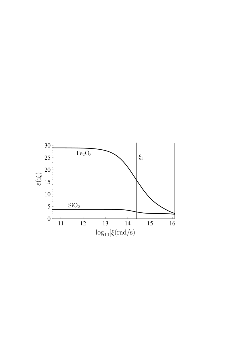
Figure 1: The dielectric permittivities of magnetite nanoparticles and silica glass are shown as the functions of imaginary frequency by the top and bottom lines, respectively. The vertical line indicates the position of the first Matsubara frequency.

As is seen from Eqs. (1)–(4), calculation of the Casimir pressure in the three-layer system is straightforward if one knows the dielectric and magnetic properties of all layers described by the functions $\varepsilon(i\xi_{l})$, $\varepsilon_{\rm ff}(i\xi_{l})$ and $\mu_{\rm ff}(i\xi_{l})$. The dielectric permittivity $\varepsilon(i\xi)$ of a silica glass, considered in the next sections as the material of walls, has been much studied b2 ; b36 . It is shown by the bottom line in Fig. 1 as the function of $\xi$. Specifically, at zero frequency one has $\varepsilon(0)=3.801$. The ferrofluid is a binary mixture of nanoparticles plus a carrier liquid. Here, we consider the dielectric and magnetic properties of magnetite Fe₃O₄ nanoparticles which make an intervening liquid stratum magnetic.

The real and imaginary parts of the dielectric permittivity of magnetite $\varepsilon_{m}(\omega)$ have been measured in a Ref. b37 in the frequency region from $\Omega_{1}=2\times 10^{14}$ rad/s to $\Omega_{2}=1.8\times 10^{16}$ rad/s (i.e., from $\hbar\Omega_{1}=0.13$ eV to $\hbar\Omega_{2}=12$ eV). We have extrapolated the measurement results of Ref. b37 for ${\rm Im}\varepsilon_{m}(\omega)$ to the region of lower frequencies $\omega<\Omega_{1}$ by using the imaginary part of the Debye permittivity

$${\rm Im}\varepsilon_{m}(\omega)=\frac{C_{D}\,\omega_{D}\,\omega}{\omega_{D}^{2}+\omega^{2}}.$$ (5)

The values of two parameters $C_{D}=24.02$ and $\omega_{D}=2.05\times 10^{14}$ rad/s were determined from the condition of smooth joining between the measured data and the Debye extrapolation. An extrapolation to the region of higher frequencies $\omega>\Omega_{2}$ was done by means of the standard theoretical dependence

$${\rm Im}\varepsilon_{m}(\omega)=C\left(\frac{\Omega_{2}}{\omega}\right)^{3},$$ (6)

where the experimental data at high frequencies lead to $C=1.58$.

Now we substitute Eqs. (5) and (6) in the right-hand side of the Kramers-Kronig relation b2 and obtain

$$\varepsilon_{m}(i\xi)=1+\frac{2}{\pi}\left[I_{1}(\xi)+I_{2}(\xi)+I_{3}(\xi)\right],$$ (7)

where

$$I_{1}(\xi)=C_{D}\omega_{D}\int_{0}^{\Omega_{1}}\frac{\omega^{2}d\omega}{(\omega_{D}^{2}+\omega^{2})(\xi^{2}+\omega^{2})},$$

$$I_{2}(\xi)=\int_{\Omega_{1}}^{\Omega_{2}}\frac{\omega{\rm Im}\varepsilon_{m}(\omega)}{\xi^{2}+\omega^{2}}d\omega,$$ (8)

$$I_{3}(\xi)=C\Omega_{2}^{3}\int_{\Omega_{2}}^{\infty}\frac{d\omega}{\omega^{2}(\xi^{2}+\omega^{2})}$$

and ${\rm Im}\varepsilon_{m}(\omega)$ in $I_{2}(\xi)$ is given by the measurement data of Ref. b37 .

Calculating the integrals $I_{1}(\xi)$ and $I_{3}(\xi)$, one finds

$$I_{1}(\xi)=\frac{C_{D}\omega_{D}^{2}}{\xi^{2}-\omega_{D}^{2}}\left[\frac{\xi}{\omega_{D}}\text{arctan}\frac{\Omega_{1}}{\xi}-\text{arctan}\frac{\Omega_{1}}{\omega_{D}}\right],$$

$$I_{3}(\xi)=\frac{C\Omega_{2}^{2}}{\xi^{2}}\left[1+\frac{\Omega_{2}}{\xi}\text{arctan}\frac{\Omega_{2}}{\xi}-\frac{\pi}{2}\right].$$ (9)

Note that in the limiting case $\xi/\Omega_{2}\ll 1$ one has

$$I_{3}(\xi)=\frac{1}{3}C\left(1-\frac{3}{5}\frac{\xi^{2}}{\Omega_{2}^{2}}+\frac{3}{7}\frac{\xi^{4}}{\Omega_{2}^{4}}\right),$$ (10)

and, thus, $I_{3}(0)=C/3\approx 0.53$. This is much smaller than $I_{1}(0)=C_{D}\text{arctan}(\Omega_{1}/\omega_{D})\approx 18.38$ and, as it follows from numerical computations, than $I_{2}(0)\approx 25.07$. In such a manner the region of high real frequencies gives only a minor contribution to $\varepsilon_{m}(0)=29.0$.

Using Eqs. (7) and (8) we have calculated $\varepsilon_{m}$ as a function of $\xi$. The computational results are shown by the top line in Fig. 1. In the same figure, the position of the first Matsubara frequency $\xi_{1}$ is indicated by the vertical line. Note that in the region of very low frequencies $\omega\lesssim 10^{3}$ Hz the dielectric permittivity of magnetite increases significantly together with its electric conductivity b38 . An increase of ${\rm Im}\varepsilon_{m}(\omega)$ at so low frequencies does not influence on the values of $\varepsilon_{m}(i\xi)$ in the frequency region shown in Fig. 1 and, hence, on the values of $\varepsilon_{m}(i\xi_{l})$ with $l\geqslant 1$. The conductivity of magnetite at low frequencies makes an impact only on the term of Eq. (1) with $l=0$ leading to $\varepsilon_{m}(\xi)\rightarrow\infty$ when $\xi\rightarrow 0$. Below in Secs. III and IV we consider both options $\varepsilon_{m}(0)=29.0$ and $\varepsilon_{m}(0)=\infty$ and adduce the arguments why the former option is more realistic in computation of the Casimir pressure.

To obtain the dielectric permittivity of the ferrofluid, $\varepsilon_{\rm ff}$, one should combine the dielectric permittivity of a carrier liquid, $\varepsilon_{c}$, with the dielectric permittivity of magnetic nanoparticles, $\varepsilon_{m}$, taking into account the volume fraction of the latter $\Phi$ in the ferrofluid. The permittivity $\varepsilon_{c}$ is discussed in Secs. III and IV for different carrier liquids. As to the combination law, for the case of spherical nanoparticles it is given by the Rayleigh mixing formula b39 used here for $\omega=i\xi$

$$\frac{\varepsilon_{\rm ff}{(i\xi)}-\varepsilon_{c}{(i\xi)}}{\varepsilon_{\rm ff}{(i\xi)}+2\varepsilon_{c}{(i\xi)}}=\Phi\frac{\varepsilon_{m}{(i\xi)}-\varepsilon_{c}{(i\xi)}}{\varepsilon_{m}{(i\xi)}+2\varepsilon_{c}{(i\xi)}}.$$ (11)

Note that Eq. (11) is derived under a condition that the nanoparticles diameter is $d\ll\lambda$, where $\lambda$ is the characteristic wavelength. In the region of separations $a\geqslant 200~{}$nm considered below the contributing frequencies are $\xi\lesssim 10^{16}~{}$rad/s which correspond to the wavelengths $\lambda\gtrsim 180~{}$nm. Thus, for nanoparticles with $d<20$ nm diameter the above condition is largely satisfied. As mentioned in Sec. I, magnetic nanoparticles may be coated with some surfactant to prevent their agglomeration. Below we assume that the dielectric function of a surfactant is close to that of a carrier liquid so that ferrofluid can be considered as a mixture of two substances.

Now we consider the magnetic permeability of a ferrofluid $\mu_{\rm ff}(i\xi_{l})$. First of all it should be stressed that the magnetic properties influence the Casimir force only through the zero-frequency term of the Lifshitz formula b40 . This is because at room temperature the magnetic permeability turns into unity at much smaller frequencies than the first Matsubara frequency. Thus, the quantity of our interest is

$$\mu_{\rm ff}(0)=1+4\pi\chi_{\rm ff}(0),$$ (12)

where the initial susceptibility of a paramagnetic (superparamagnetic) system is given by b41

$$\chi_{\rm ff}(0)=N\frac{M^{2}}{3k_{B}T},$$ (13)

where $N=\Phi/V$, $V=\pi d^{3}/6$ is the volume of a single-domain nanoparticle, $M=M_{S}V$ is its magnetic moment, and $M_{S}$ is the saturation magnetization per unit volume.

It was found that for nanoparticles $M_{S}$ takes a smaller value than for a bulk material. Thus, for a bulk magnetite $M_{S}\approx~{}460~{}\mbox{emu/cm}^{3}=4.6\times 10^{5}~{}$A/m b42 , whereas for a single magnetite nanoparticle $M_{S}\approx 300~{}\mbox{emu/cm}^{3}=3\times 10^{5}~{}$A/m b43 . Substituting Eq. (13) in Eq. (12), we arrive at

$$\mu_{\rm ff}(0)=1+\frac{2\pi^{2}\Phi}{9}\frac{M_{S}^{2}d^{3}}{k_{B}T}.$$ (14)

From this equation with the volume fraction of nanoparticles $\Phi=0.05$ one finds $\mu_{\rm ff}(0)\approx 1.24$ and $2.9$ for magnetite nanoparticles with $d=10$ and $20$ nm diameter, respectively. These results do not depend on the type of carrier liquid.

III Impact of magnetite nanoparticles on the Casimir
pressure in kerosene-based interlayer

Kerosene is often used as a carrier liquid in ferrofluids b44 ; b45 . By now the dielectric properties of kerosene are not sufficiently investigated. We have applied the measurement data for the imaginary part of the dielectric permittivity of kerosene in the microwave b44 and infrared b46 regions and the Kramers-Kronig relation to obtain the Ninham-Parsegian representation for this dielectric permittivity along the imaginary frequency axis

$$\varepsilon_{c}(i\xi)=1+\frac{B}{1+\xi\tau}+\frac{C_{\rm IR}}{1+(\frac{\xi}{\omega_{\rm IR}})^{2}}+\frac{C_{\rm UV}}{1+(\frac{\xi}{\omega_{\rm UV}})^{2}}.$$ (15)

Here, the second term on the right-hand side describes the contribution to the dielectric permittivity from the orientation of permanent dipoles in polar liquids. The value of $B=0.020$ and $1/\tau=8.0\times 10^{8}$ rad/s were determined from the measurement data of Ref. b44 in the microwave region. The third term on the right-hand side of Eq. (15) describes the effect of ionic polarization. The respective constants $C_{\rm IR}=0.007$ and $\omega_{\rm IR}=2.14\times 10^{14}$ rad/s were found using the infrared optical data b46 . Taking into account that for kerosene the optical data in the ultraviolet region are missing, the parameters of the last, fourth, term on the right-hand side of Eq. (15) have been determined following the approach of Ref. b36 with regard to the known value of the dielectric permittivity of zero-frequency $\varepsilon_{c}(0)=1.8$ b44 . As a result, the values of $C_{\rm UV}=0.773$ and $\omega_{\rm UV}=1.0\times 10^{16}$ rad/s were obtained.

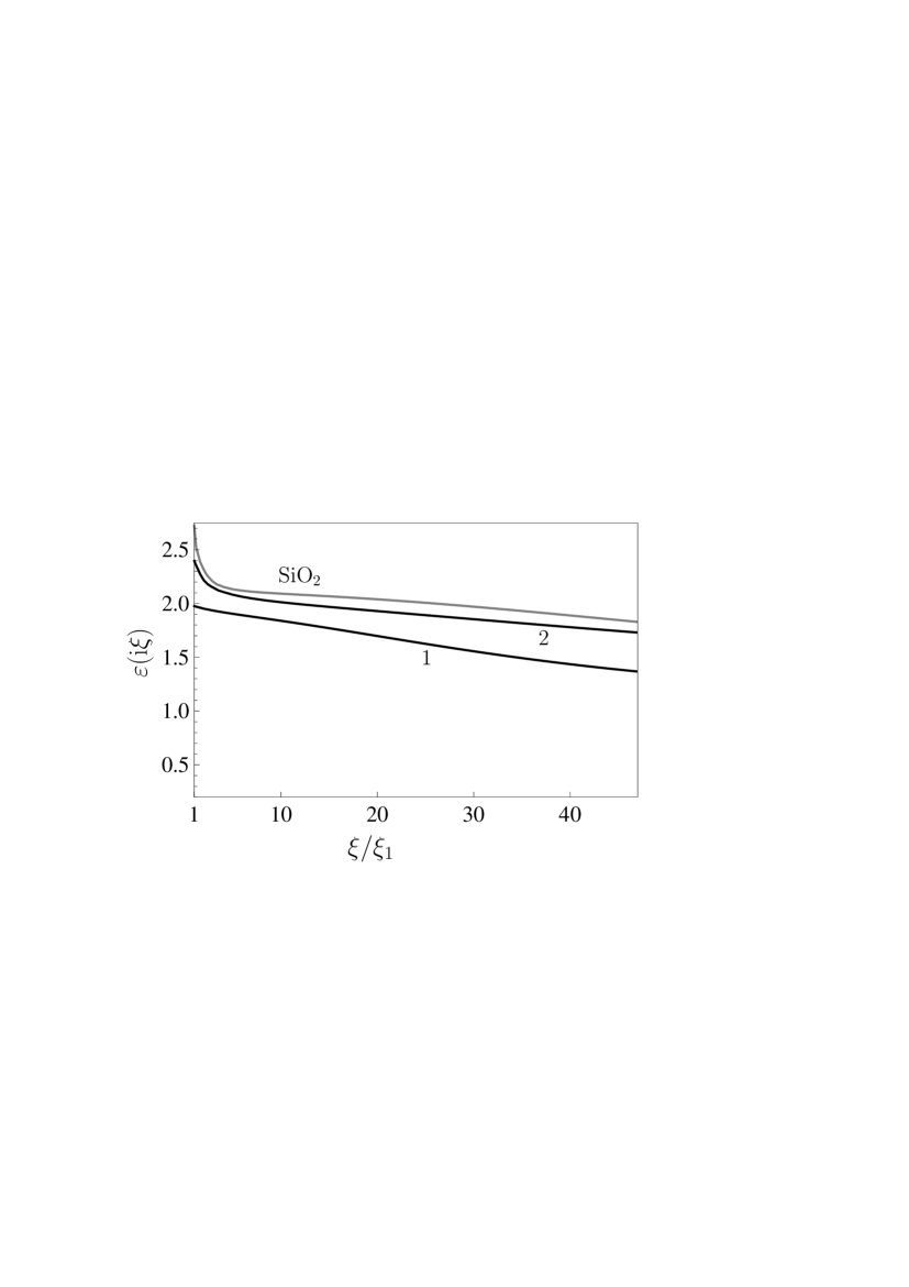
Figure 2: The dielectric permittivities of the kerosene- and water-based ferrofluids with 5$\%$ concentration of magnetite nanoparticles (the lines 1 and 2, respectively) and of silica glass are shown as the functions of imaginary frequency normalized to the first Matsubara frequency.

Now the dielectric permittivity $\varepsilon_{\rm ff}(i\xi)$ of kerosene-based ferrofluid with $\Phi=0.05~{}(5\%)$ volume fraction of magnetite nanoparticles is obtained from Eq. (11) by substituting the data of the top line in Fig. 1 for the dielectric permittivity of magnetite $\varepsilon_{m}(i\xi)$ and the dielectric permittivity of kerosene $\varepsilon_{c}(i\xi)$ from Eq. (15). The permittivity $\varepsilon_{\rm ff}$ is shown as a function of $\xi/\xi_{1}$ by the line labeled 1 in Fig. 2. In the same figure the dielectric permittivity of SiO₂ walls is reproduced by the top line from Fig. 1 as a function of $\xi/\xi_{1}$ in the frequency region important for computations of the Casimir pressure (the line labeled 2 in Fig. 2 is discussed in Sec. IV). The static dielectric permittivity of a ferrofluid, which is not shown in the scale of Fig. 2, is equal to $\varepsilon_{\rm ff}(0)=2.035$ if the conductivity of magnetite nanoparticles is disregarded and $\widetilde{\varepsilon}_{\rm ff}(0)=2.084$ if this conductivity is included in calculations.

Numerical computations of the Casimir pressure are performed most conveniently by using the dimensionless variables

$$y=2ak_{\rm ff}(i\xi_{l},k_{\bot}),\quad\zeta_{l}=\frac{\xi_{l}}{\omega_{\rm cr}}\equiv\frac{2a\xi_{l}}{c}.$$ (16)

In terms of these variables Eq. (1) takes the form

$${P}(a)=-\frac{k_{B}T}{8{\pi}a^{3}}\sum_{l=0}^{\infty}\vphantom{\sum}{}^{{}^{\prime}}\int_{\sqrt{\varepsilon_{{\rm ff},l}\mu_{{\rm ff},l}}\zeta_{l}}^{\infty}y^{2}dy$$ (17)

$$~{}~{}~{}\times\sum_{\alpha}\left[\frac{e^{y}}{r^{2}_{\alpha}(i{\zeta}_{l},y)}-1\right]^{-1},$$

where $\varepsilon_{{\rm ff},l}=\varepsilon_{\rm ff}(i\omega_{\rm cr}\zeta_{l})$, $\mu_{{\rm ff},l}=\mu_{\rm ff}(i\omega_{\rm cr}\zeta_{l})$ and the reflection coefficients (3) are given by

$$r_{\rm TM}(i\zeta_{l},y)=\frac{\varepsilon_{l}y-\varepsilon_{{\rm ff},l}\sqrt{y^{2}+(\varepsilon_{l}-\varepsilon_{{\rm ff},l}\mu_{{\rm ff},l})\zeta_{l}^{2}}}{\varepsilon_{l}y+\varepsilon_{{\rm ff},l}\sqrt{y^{2}+(\varepsilon_{l}-\varepsilon_{{\rm ff},l}\mu_{{\rm ff},l})\zeta_{l}^{2}}},$$

$$r_{\rm TE}(i\zeta_{l},y)=\frac{y-\mu_{{\rm ff},l}\sqrt{y^{2}+(\varepsilon_{l}-\varepsilon_{{\rm ff},l}\mu_{{\rm ff},l})\zeta_{l}^{2}}}{y+\mu_{{\rm ff},l}\sqrt{y^{2}+(\varepsilon_{l}-\varepsilon_{{\rm ff},l}\mu_{{\rm ff},l})\zeta_{l}^{2}}}.$$ (18)

with a similar notation for $\varepsilon_{l}=\varepsilon(i\omega_{\rm cr}\zeta_{l})$.

The magnitude of the Casimir pressure between two SiO₂ walls through the kerosene-based ferrofluid was computed by using Eqs. (17) and (18) where the dielectric permittivities of SiO₂ and of a ferrofluid are given by the top line and line 1 in Fig. 2, respectively. The magnetic permeability of a ferrofluid obtained from Eq. (14) in the end of Sec. II has been used. The computational results are shown in Fig. 3 as functions of separation by the pair of solid lines labeled 1 where the lower and upper lines are for magnetite nanoparticles with $d=10$ and $20$ nm diameter, respectively. (The pair of lines labeled 2 is discussed in Sec. IV). Note that the dielectric permittivities used in computations do not depend on the nanoparticle diameter $d$ which influences the computational results exclusively through the static magnetic permeability of the ferrofluid.

The solid lines in pair 1 are calculated with disregarded conductivity of magnetite at low frequencies, i.e., by using the static dielectric permittivity of a ferrofluid $\varepsilon_{\rm ff}(0)=2.035$. The point is that the theoretical results obtained with taken into account conductivity of dielectric materials at low frequencies have been found in serious disagreement with the experimental data of several measurements of the Casimir force b2 ; b5 ; b47 ; b48 ; b49 ; b50 ; b51 ; b52 . Moreover, the Casimir entropy calculated with included conductivity at low frequencies was demonstrated to violate the third law of thermodynamics, the Nernst heat theorem, by taking nonzero positive value depending on the parameters of a system at zero temperature b53 ; b54 ; b55 ; b56 . Since the deep physical reasons for this experimental and theoretical conundrum remain unknown, here the computations of the Casimir pressure are also performed with taken into account conductivity of magnetite at low frequencies.

The respective computational results are shown in Fig. 3 by the pair of dashed lines labeled 1. The lower and upper dashed lines are computed using the same expressions, as the solid lines, but by using the static dielectric permittivity of magnetite $\tilde{\varepsilon}_{\rm ff}(0)=2.084$ for nanoparticles with $d=10$ and $20$ nm, respectively. As is seen in Fig. 3, an account for the conductivity of magnetite at low frequencies makes only a minor impact on the Casimir pressure in the three-layer system. Thus, for nanoparticles with $d=10$ nm diameter the pressures computed at $a=200$ nm with disregarded and included conductivity at low frequencies are equal to $P=-3.789$ mPa and $\tilde{P}=-3.653$ mPa. At $a=2~{}\mu$m similar results are given by $P=-2.24\times 10^{-3}$ mPa and $\widetilde{P}=-2.104\times 10^{-3}$ mPa. For magnetite nanoparticles with $d=20$ nm diameter the Casimir pressures computed with disregarded and included conductivity at low frequencies are $P=-8.598$ mPa and $\tilde{P}=-8.462$ mPa at $a=200$ nm and $P=-7.049\times 10^{-3}$ mPa and $\tilde{P}=-6.913\times 10^{-3}$ mPa at $a=2~{}\mu$m.

It is interesting to determine the relative impact of magnetite nanoparticles on the magnitude of the Casimir pressure in a three-layer system. For this purpose we have computed the quantity

$$\delta|P|=\frac{|P|-|P_{\rm ker}|}{|P_{\rm ker}|},$$ (19)

where $|P_{\rm ker}|$ is the magnitude of the Casimir pressure between two SiO₂ walls through a pure kerosene stratum with no nanoparticles. The computational results for the quantity $\delta|P|$ are shown in Fig. 4 as the functions of separation by the pairs of line labeled 1 and 2 for nanoparticles of $d=10$ and $20$ nm diameter, respectively. The solid and dashed lines in each pair are computed with disregarded and included conductivity of magnetite at low frequencies, respectively. As is seen in Fig. 4, on addition of magnetite nanoparticles with $d=10$ nm diameter to kerosene, the magnitude of the Casimir pressure decreases. However, on addition to kerosene of nanoparticles with by a factor of two larger diameter, the magnitude of the Casimir pressure increases. Specifically, at $a=200$ nm one obtains $\delta|P|=-38.7\%$ and $40.05\%$ for nanoparticles with $d=10$ and $20$ nm if the conductivity at low frequencies is disregarded in computations. If this conductivity is taken into account, the respective results are $\delta|\tilde{P}|=-40.9\%$ and $37.8\%$. The relative impact of magnetic nanoparticles on the Casimir pressure essentially depends on the separation between the plates. Thus, at $a=2~{}\mu$m $\delta|P|=-22.0\%$ and $147\%$ for nanoparticles with $d=10$ and $20$ nm if the conductivity of magnetite is disregarded and $\delta|\widetilde{P}|=-26.8\%$ and $142\%$ for the same respective diameters if the conductivity is included in computations.

Next we consider the relative difference in the magnitudes of the Casimir pressure on an addition of magnetite nanoparticles to kerosene as a function of nanoparticle diameter. The computational results are shown in Fig. 5 by the solid and dashed lines computed with disregarded and included conductivity of magnetite at low frequencies, respectively, for separation between the walls (a) $200$ nm and (b) $2~{}\mu$m.

From Fig. 5(a,b) it is seen that at both separations considered the relative change in the magnitude of the Casimir pressure is a monotonously increasing function of the nanoparticle diameter $d$ which changes its sign and takes the zero value for some $d$. Thus, from Fig. 5(a) one concludes that at $a=200$ nm $\delta|P|=0$ for $d=16.6$ nm if the conductivity of magnetite at low frequencies is disregarded in computations and for $d=16.8$ nm if it is taken into account. This means that at $a=200$ nm an inclusion in kerosene of nanoparticles with some definite diameter does not make any impact on the Casimir pressure. According to Fig. 5(b), similar situation holds at $a=2~{}\mu$m. Here, $\delta|P|=0$ for $d=12.9$ and $13.3$ nm depending on whether the conductivity of magnetite at low frequencies is disregarded or included in computations.

The obtained results can be qualitatively explained by the fact that for magnetic materials with $\mu>1$ the magnitude of the Casimir pressure is always larger, as compared to materials with $\mu=1$. On the other hand, the presence of magnetite nanoparticles in kerosene influences on its dielectric permittivity in such a way that the magnitude of the Casimir pressure decreases. These two tendencies act in the opposite directions and may nullify an impact of magnetic nanoparticles with some definite diameter on the Casimir pressure.

IV The Case of Water-based Interlayer

In this section we consider the Casimir pressure in the three-layer system where an interlayer is formed by the water-based ferrofluid. Water is of frequent use as a carrier liquid (see, e.g., Refs. b57 ; b58 ; b59 ). The dielectric permittivity of water along the imaginary frequency axis is well described in the oscillator representation b60

$$\varepsilon_{c}(i\xi)=1+\frac{B}{1+\xi\tau}+\sum_{j=1}^{11}\frac{C_{j}}{1+(\frac{\xi}{\omega_{j}})^{2}+g_{j}\frac{\xi}{\omega_{j}^{2}}},$$ (20)

where the second term on the right hand-side of this equation describes the contribution from the orientation of permanent dipoles. Specifically, for water one has $B=76.8$ and $1/\tau=1.08\times 10^{11}$ rad/s. The oscillator terms with $g=1,\,2,...,\,6$ represent the effects of electronic polarization. The respective oscillator frequencies belong to the ultraviolet spectrum: $\omega_{j}=1.25\times 10^{16},\ 1.52\times 10^{16},\ 1.73\times 10^{16},\ 2.07\times 10^{16},\ 2.70\times 10^{16}$ and $3.83\times 10^{16}$ rad/s. The oscillator strength and relaxation parameters of these oscillators are given by: $C_{j}=0.0484,\ 0.0387,\ 0.0923,\ 0.344,\ 0.360,\ 0.0383$ and $g_{j}=0.957\times 10^{15},\ 1.28\times 10^{15},\ 3.11\times 10^{15},\ 5.92\times 10^{15},\ 11.1\times 10^{15},\ 8.11\times 10^{15}$ rad/s. The terms of Eq. (20) with $j=7,\,8,...,\,11$ represent the effects of ionic polarization and their frequencies belong to the infrared spectrum: $\omega_{j}=0.314\times 10^{14},\ 1.05\times 10^{14},\ 1.40\times 10^{14},\ 3.06\times 10^{14},\ 6.46\times 10^{14}$ rad/s. The respective oscillator strengths and relaxation parameters take the following values: $C_{j}=1.46,\ 0.737,\ 0.152,\ 0.0136,\ 0.0751$ and $g_{j}=2.29\times 10^{13},\ 5.78\times 10^{13},\ 4.22\times 10^{13},\ 3.81\times 10^{13},\ 8.54\times 10^{13}$ rad/s b60 .

Using the dielectric permittivity $\varepsilon_{c}$ of water (20) and the dielectric permittivity of magnetite nanoparticles $\varepsilon_{m}$ given by the top line in Fig. 1, the permittivity $\varepsilon_{\rm ff}(i\xi)$ of the water-based ferrofluid with $\Phi=0.05$ fraction of nanoparticles is obtained from Eq. (11). It is shown by the line labeled 2 in Fig. 2 as a function of the imaginary frequency normalized to the first Matsubara frequency. The dielectric permittivity of the water-based ferrofluid at zero Matsubara frequency is equal to $77.89$ if the conductivity of magnetite at low frequencies is disregarded and to $93.97$ if it is taken into account in calculations.

The magnitude of the Casimir pressure between two SiO₂ walls through the water-based ferrofluid was computed similar to Sec. III by using Eqs. (17) and (18) and all respective dielectric permittivities and magnetic permeabilities defined along the imaginary frequency axis. The computational results are shown in Fig. 3 as functions of separation by the pair of solid lines labeled 2 where the lower and upper lines are computed for magnetite nanoparticles with $d=10$ and $20$ nm diameter, respectively. Similar to Sec. III, the conductivity of magnetite at low frequencies was first disregarded. Then the computations have been repeated with taken into account conductivity. The obtained results are shown by the pair of dashed lines labeled 2. As is seen in Fig. 3, an account of the conductivity of magnetite makes only a minor impact on the Casimir pressure. Thus, for $d=10$ nm, $a=200~{}$nm one obtains $P=-19.82$ mPa and $\tilde{P}=-20.61$ mPa with disregarded and included conductivity of magnetite, respectively. At larger separation $a=2~{}\mu$m similar results are $P=-1.964\times 10^{-2}$ mPa and $\tilde{P}=-2.043\times 10^{-2}$ mPa. For nanoparticles of $d=20$ nm diameter we find $P=-24.62$ mPa and $\tilde{P}=-25.42$ mPa at $a=200$ nm and $P=-2.444\times 10^{-2}$ mPa, $\tilde{P}=-2.524\times 10^{-2}$ mPa at $a=2~{}\mu$m.

The relative impact of magnetite nanoparticles on the Casimir pressure in three-layer system with a water interlayer can be calculated by Eq. (19) where $|P_{\rm ker}|$ should be replaced with $|P_{\rm wat}|$ found for a pure water stratum sandwiched between two SiO₂ walls. The computational results are shown in Fig. 6 as functions of separation by the lines labeled 1 and 2 for nanoparticles with $d=10$ and $20$ nm diameter, respectively. As above, the solid and dashed lines in each pair are computed with disregarded and included conductivity of magnetite, respectively.

From Fig. 6 it is seen that on addition of nanoparticles with $d=20$ nm diameter to water the magnitude of the Casimir pressure increases independently of whether the conductivity of magnetite is disregarded or included in computations. The same is true for nanoparticles of $d=10$ nm diameter, but only under a condition that the conductivity of magnetite is taken into account. If the conductivity is disregarded for nanoparticles with $d=10$ nm (the solid line labeled 1), the quantity $\delta|P|$ takes the negative values over the wide separation range, i.e., on addition of magnetite nanoparticles to water the magnitude of the Casimir pressure becomes smaller.

At $a=200$ nm one obtains $\delta|P|=-3.3\%$ and $20.4\%$ for nanoparticles with $d=10$ and 20 nm diameter, respectively, and $\delta|\tilde{P}|=0.58\%$ and $24.3\%$ for the same respective diameters. At $a=2~{}\mu$m similar results are the following: $\delta|P|=0.12\%$ and $24.9\%$, and $\delta|\tilde{P}|=4.2\%$ and $29.0\%$ for $d=10$ and 20 nm, respectively.

In the end of this section, we calculate the relative difference in Casimir pressures $\delta|P|$ for a water-based ferrofluid as a function of nanoparticle diameter. In Fig. 7 the computational results are presented by the solid and dashed lines computed with disregarded and included conductivity of magnetite, respectively, for separation between the walls $a=200$ nm in Fig. 7(a) and $a=2~{}\mu$m in Fig. 7(b).

As can be seen in Fig. 7, for a water-based ferrofluid the quantity $\delta|P|$ is again the monotonously increasing function of nanoparticle diameter $d$ which changes its sign for some value of $d$. According to Fig. 7(a), at $a=200$ nm and Casimir pressure does not change on an addition of magnetite nanoparticles with $d=13$ nm diameter to water if the conductivity at low frequencies is disregarded. If it is included in computations, the value of this diameter is reduced to $d=8.8$ nm. If the separation distance between SiO₂ walls is $a=2~{}\mu$m, an addition to water of magnetite nanoparticles with $d=9.8$ nm diameter does not make an impact to the Casimir pressure under a condition that the conductivity of magnetite is disregarded. If this conductivity is included in computations, an addition of nanoparticles of any diameter to water influences the Casimir pressure in the three-layer system. The qualitative explanation of this effect is the same as considered in Sec. III for the kerosene-based ferrofluids.

V Conclusions and Discussion

In the foregoing, we have considered the Casimir pressure in three-layer systems where the intervening stratum processes magnetic properties. This subject has assumed importance in the context of ferrofluids and their extensive use in micromechanical sensors and other prospective applications discussed in Sec. I. Taking into account that the magnetic properties of ferrofluids and determined by some fraction of magnetic nanoparticles added to a nonmagnetic (carrier) liquid, we have investigated an impact of such nanoparticles with different diameters of the Casimir pressure.

After presenting the general formalism of the Lifshitz theory adapted to this case, we have found the dielectric permittivity and the magnetic permeability of magnetite nanoparticles along the imaginary frequency axis on the basis of available optical data. Specific computations have been performed for the kerosene- and water-based ferrofluids which are most commonly studied in the literature. For this purpose, we have constructed the dielectric permittivity of kerosene using its measured optical properties in the microwave and infrared regions and employed the familiar representation for the dielectric permittivity of water. These permittivities have been combined with the permittivity of magnetite nanoparticles by using the Rayleigh mixing formula to obtain the dielectric permittivities of ferrofluids with 5$\%$ concentration of nanoparticles.

The Casimir pressure was computed for the three-layer systems consisting of two parallel SiO₂ walls with an intervening stratum of either kerosene- or water-based ferrofluid as a function of separation between the walls. We have also computed the relative difference in the magnitudes of the Casimir pressure on addition of the $5\%$ fraction of magnetic nanoparticles to the pure kerosene and water as a function of separation and nanoparticle diameter. It was shown that this relative difference is rather large and should be taking into account. As an example, for kerosene- and water-based ferrofluids with nanoparticles of 20 nm diameter sandwiched between two SiO₂ walls 2 $\mu$m apart, the relative change in the magnitude of the Casimir pressure exceeds 140$\%$ and 25$\%$, respectively.

All computations have been performed in the framework of two theoretical approaches to the Casimir force developed in the literature during the last twenty years and used for comparison between experiment and theory. It turned out that both of these approaches lead to fairly close predictions for the magnitudes of the Casimir pressure in three-layer systems through a ferrofluid interlayer. In doing so, theoretical predictions for the relative change in the magnitude of the Casimir pressure on addition of magnetic nanoparticles to a carrier liquid is more sensitive to the approach used and may vary in the limits of several percent.

An interesting effect found for the three-layer systems with a ferrofluid intervening stratum is that at fixed separation between the walls an addition of magnetite nanoparticles with some definite diameter to a carrier liquid makes no impact on the Casimir pressure between SiO₂ walls. The respective diameters are found for both kerosene- and water-based ferrofluids. The quantitative physical explanation for this effect is provided.

In conclusion, it may be said that the above results open opportunities for precise control of the Casimir force in the three-layer systems with a magnetic intervening stratum, which may be used in the next generation of ferrofluid-based microdevices.

VI Acknowledgments

The work of V. M. M. was partially supported by the Russian Government Program of Competitive Growth of Kazan Federal University.

                      

                      

                      

Figure 3: The magnitudes or the Casimir pressure between SiO₂ walls through a ferrofluid with 5$\%$ fraction of magnetite nanoparticles are shown as the functions of separation between the walls by the pairs of solid and dashed lines labeled 1 and 2 for the kerosene and water carrier liquids, respectively. Solid and dashed lines are computed with disregarded and included conductivity of magnetite at low frequencies, respectively. In each pair the lower line is for nanoparticles with $d=10$ nm diameter and the upper line is for nanoparticles with $d=20$ nm.

                      

Figure 4: The relative change in the magnitude of the Casimir pressure on addition of the 5$\%$ fraction of magnetite nanoparticles to kerosene is shown as the function of separation by the pairs of solid and dashed lines labeled 1 and 2 for nanoparticles with $d=10$ nm and 20 nm diameter, respectively. In each pair, the solid and dashed lines are computed with disregarded and included conductivity of magnetite at low frequencies, respectively.

                      

Figure 5: The relative change in the magnitude of the Casimir pressure on addition of the 5$\%$ fraction of magnetite nanoparticles to kerosene is shown as the function of nanoparticle diameter by the pairs of solid and dashed lines computed with disregarded and included conductivity of magnetite at low frequencies, respectively, for separation between SiO₂ walls (a) 200 nm and (b) 2 $\mu$m.

                      

Figure 6: The relative change in the magnitude of the Casimir pressure on addition of the 5$\%$ fraction of magnetite nanoparticles to water is shown as the function of separation by the pairs of solid and dashed lines labeled 1 and 2 for nanoparticles with $d=10$ and 20 nm diameter, respectively. In each pair, the solid and dashed lines are computed with disregarded and included conductivity of magnetite at low frequencies, respectively.

                      

Figure 7: The relative change in the magnitude of the Casimir pressure on addition of the 5$\%$ fraction of magnetite nanoparticles to water is shown as the function of nanoparticle diameter by the solid and dashed lines computed with disregarded and included conductivity of magnetite at low frequencies, respectively, for separation between SiO₂ walls (a) 200 nm and (b) 2 $\mu$m.

References

- (1) V. A. Parsegian, van der Waals Forces: A Handbook for Biologists, Chemists, Engineers, and Physicists (Cambridge University Press, Cambridge, 2005).
- (2) M. Bordag, G. L. Klimchitskaya, U. Mohideen, and V. M. Mostepanenko, Advances in the Casimir Effect (Oxford University Press, Oxford, 2015).
- (3) E. M. Lifshitz, The theory of molecular attractive forces between solids, Zh. Eksp. Teor. Fiz. 29, 94 (1955) [Sov. Phys. JETP 2, 73 (1956)].
- (4) I. E. Dzyaloshinskii, E. M. Lifshitz, and L. P. Pitaevskii, The general theory of van der Waals forces, Usp. Fiz. Nauk 73, 381 (1961) [Adv. Phys. 10, 165 (1961)].
- (5) G. L. Klimchitskaya, U. Mohideen, and V. M. Mostepanenko, The Casimir force between real materials: Experiment and theory, Rev. Mod. Phys. 81, 1827 (2009).
- (6) G. L. Klimchitskaya, U. Mohideen, and V. M. Mostepanenko, Control of the Casimir force using semiconductor test bodies, Int. J. Mod. Phys. B 25, 171 (2011).
- (7) A. A. Banishev, C.-C. Chang, G. L. Klimchitskaya, V. M. Mostepanenko, and U. Mohideen, Measurement of the gradient of the Casimir force between a nonmagnetic gold sphere and a magnetic nickel plate, Phys. Rev. B 85, 195422 (2012).
- (8) A. A. Banishev, G. L. Klimchitskaya, V. M. Mostepanenko, and U. Mohideen, Demonstration of the Casimir Force Between Ferromagnetic Surfaces of a Ni-Coated Sphere and a Ni-Coated Plate, Phys. Rev. Lett. 110, 137401 (2013).
- (9) A. A. Banishev, G. L. Klimchitskaya, V. M. Mostepanenko, and U. Mohideen, Casimir interaction between two magnetic metals in comparison with nonmagnetic test bodies, Phys. Rev. B 88, 155410 (2013).
- (10) G. Bimonte, D. López, and R. S. Decca, Isoelectronic determination of the thermal Casimir force, Phys. Rev. B 93, 184434 (2016).
- (11) J. N. Munday, F. Capasso, V. A. Parsegian, and S. M. Bezrukov, Measurement of the Casimir-Lifshitz force in a fluid: The effect of electrostatic forces and Debye screening, Phys. Rev. A 78, 032109 (2008).
- (12) J. N. Munday, F. Capasso, and V. A. Parsegian, Measured long-range repulsive Casimir -Lifshitz forces, Nature 457, 170 (2009).
- (13) A. W. Rodriguez, F. Capasso, and S. G. Johnson, The Casimir effect in microstructured geometries, Nat. Photonics 5, 211 (2011).
- (14) H. B. Chan, V. A. Aksyuk, R. N. Kleiman, D. J. Bishop, and F. Capasso, Quantum mechanical actuation of microelectromechanical systems by the Casimir force, Science 291, 1941 (2001).
- (15) H. B. Chan, V. A. Aksyuk, R. N. Kleiman, D. J. Bishop, and F. Capasso, Nonlinear Micromechanical Casimir Oscillator, Phys. Rev. Lett. 87, 211801 (2001).
- (16) J. Barcenas, L. Reyes, and R. Esquivel-Sirvent, Scaling of micro- and nanodevices actuated by the Casimir force, Appl. Phys. Lett. 87, 263106 (2005).
- (17) R. Esquivel-Sirvent and R. Pérez-Pasqual, Geometry and charge carrier induced stability in Casimir actuated nanodevices, Eur. Phys. J. B 86, 467 (2013).
- (18) W. Broer, G. Palasantzas, J. Knoester, and V. B. Svetovoy, Significance of the Casimir force and surface roughness for actuation dynamics of MEMS, Phys. Rev. B 87, 125413 (2013).
- (19) M. Sedighi, W. H. Broer, G. Palasantzas, and B. J. Kooi, Sensitivity of micromechanical actuation on amorphous to crystalline phase transformations under the influence of Casimir forces, Phys. Rev. B 88, 165423 (2013).
- (20) W. Broer, H. Waalkens, V. B. Svetovoy, J. Knoester, and G. Palasantzas, Nonlinear Actuation Dynamics of Driven Casimir Oscillators with Rough Surfaces, Phys. Rev. Appl. 4, 054016 (2015).
- (21) J. Zou, Z. Marcet, A. W. Rodriguez, M. T. H. Reid, A. P. McCauley, I. I. Kravchenko, T. Lu, Y. Bao, S. G. Johnson, and H. B. Chan, Casimir forces on a silicon micromechanical chip, Nat. Commun. 4, 1845 (2013).
- (22) L. Tang, M. Wang, C. Y. Ng, M. Nikolic, C. T. Chan, A. W. Rodriguez, and H. B. Chan, Measurement of nonmonotonic Casimir forces between silicon nanostructures, Nat. Photonics 11, 97 (2017).
- (23) N. Inui, Optical switching of a graphene mechanical switch using the Casimir effect, J. Appl. Phys. 122, 104501 (2017).
- (24) G. L. Klimchitskaya, V. M. Mostepanenko, V. M. Petrov, and T. Tschudi, Optical Chopper Driven by the Casimir Force, Phys. Rev. Applied 10, 014010 (2018).
- (25) R. E. Rosensweig, Ferrohydrodynamics (Cambridge University Press, Cambridge, 1985).
- (26) J. Philip, and J. M. Laskar, Optical properties and applications of ferrofluids — a review, J. Nanofluids 1, 3 (2012).
- (27) L. Mao, S. Elborai, X. He, M. Zahn, and H. Koser, Direct observation of closed-loop ferrohydrodynamic pumping under travelling magnetic fields, Phys. Rev. B 84, 104431 (2011).
- (28) W. Lin, Y. Miao, H. Zhang, B. Liu, Y. Liu, and B. Song, Fiber-optic in-line magnetic field sensor based on the magnetic fluid and multimode interference effects, Appl. Phys. Lett. 103, 151101 (2013).
- (29) A. V. Prokofiev, E. K. Nepomnyashchaya, I. V. Pleshakov, Yu. I. Kuzmin, E. N. Velichko, and E. T. Aksenov, Study of specific features of laser radiation scattering by aggregates of nanoparticles in ferrofluids used for optoelectronic communication systems, in “Internet of Things, Smart Spaces and Next Generation Networks and Systems”, edited by O. Galinina, S. Balandin, and Y. Koucheryavy, (Springer, Cham, 2016), pp. 680.
- (30) E. K. Nepomnyashchaya, E. N. Velichko, I. V. Pleshakov, E. T. Aksenov, and E. A. Savchenko, Investigation of ferrofluid nanostructure by laser light scattering: medical applications, J. Phys.: Conf. Ser. 841, 012020, (2017).
- (31) C. Goubault, P. Jop, M. Fermigier, J. Baudry, E. Bertrand, and J. Bibette, Flexible Magnetic Filaments as Micromechanical Sensors, Phys. Rev. Lett. 91, 260802 (2003).
- (32) N. Pekas, M. D. Porter, M. Tondra, A. Popple, and A. Jander, Giant magnetoresistance monitoring of magnetic picodroplets in an integrated microfluidic system, Appl. Phys. Lett. 85, 4783 (2004).
- (33) D. W. Inglis, R. Riehn, R. H. Austin, and J. C. Sturm, Continuous microfluidic immunomagnetic cell separation, Appl. Phys. Lett. 85, 5093 (2004).
- (34) N. Saga and T. Nakamura, Elucidation of propulsive force of microrobot using magnetic fluid, J. Appl. Phys. 91, 7003 (2002).
- (35) G. L. Klimchitskaya and V. M. Mostepanenko, Observability of thermal effects in the Casimir interaction from graphene-coated substrates, Phys. Rev. A 89, 052512 (2014).
- (36) D. B. Hough and L. R. White, The calculation of Hamaker constants from Liftshitz theory with applications to wetting phenomena, Adv. Colloid. Interface Sci. 14, 3 (1980).
- (37) A. Schlegel, S. F. Alvarado, and P. Wachter, Optical properties of magnetite (Fe3O4), J. Phys. C: Solid State Phys. 12, 1157 (1979).
- (38) A. Radoń, D. Łukowiec, M. Kremzer, J. Mikuła, and P. Włodarczyk, Electrical Conduction Mechanism and Dielectric Properties of Spherical Shaped Fe3O4 Nanoparticles Synthesized by Co-Precipitation Method, Materials 11, 735 (2012).
- (39) A. H. Sihvola, Electromagnetic Mixing Formulas and Applications (The Institution of Electrical Engineers, London, 1999).
- (40) B. Geyer, G. L. Klimchitskaya, and V. M. Mostepanenko, Thermal Casimir interaction between two magnetodielectric plates, Phys. Rev. B 81, 104101 (2010).
- (41) S. V. Vonsovskii, Magnetism (Wiley, New York, 1974).
- (42) S. Chikazumi and S. H. Charap, Physics of Magnetism (Wiley, New York, 1964).
- (43) S. van Berkum, J. T. Dee, A. P. Philipse, and B. E. Erné, Frequency-dependent magnetic susceptibility of magnetite and cobalt ferrite nanoparticles embedded in PAA hydrogel, Int. J. Mol. Sci. 14, 10162 (2013).
- (44) P. C. Fannin, C. N. Marin, I. Malaescu, and N. Stefu, Microwave dielectric properties of magnetite colloidal particles in magnetic fluids, J. Phys.: Condens. Matter 19, 036104 (2007).
- (45) C.-Y. Hong, I. J. Jang, H. E. Horng, C. J. Hsu, Y. D. Yao, and H. C. Yang, Ordered structures in Fe3O4 kerosene-based ferrofluids, J. Appl. Phys. 81, 4275 (1997).
- (46) H. Qi, X. Zhang, M. Jiang, Q. Wang, and D. Li, A method to determine optical properties of kerosene using transmission spectrum, Optik 127, 8899 (2016).
- (47) F. Chen, G. L. Klimchitskaya, V. M. Mostepanenko, and U. Mohideen, Demonstration of optically modulated dispersion forces, Opt. Express 15, 4823 (2007).
- (48) F. Chen, G. L. Klimchitskaya, V. M. Mostepanenko, and U. Mohideen, Control of the Casimir force by the modification of dielectric properties with light, Phys. Rev. B 76, 035338 (2007).
- (49) J. M. Obrecht, R. J. Wild, M. Antezza, L. P. Pitaevskii, S. Stringari, and E. A. Cornell, Measurement of the temperature dependence of the Casimir-Polder force, Phys. Rev. Lett. 98, 063201 (2007).
- (50) G. L. Klimchitskaya and V. M. Mostepanenko, Conductivity of dielectric and thermal atom-wall interaction, J. Phys. A: Math. Theor. 41, 312002 (2008).
- (51) C.-C. Chang, A. A. Banishev, G. L. Klimchitskaya, V. M. Mostepanenko, and U. Mohideen, Reduction of the Casimir Force from Indium Tin Oxide Film by UV Treatment, Phys. Rev. Lett. 107, 090403 (2011).
- (52) A. A. Banishev, C.-C. Chang, R. Castillo-Garza, G. L. Klimchitskaya, V. M. Mostepanenko, and U. Mohideen, Modifying the Casimir force between indium tin oxide film and Au sphere, Phys. Rev. B 85, 045436 (2012).
- (53) B. Geyer, G. L. Klimchitskaya, and V. M. Mostepanenko, Thermal quantum field theory and the Casimir interaction between dielectrics, Phys. Rev. D 72, 085009 (2005).
- (54) B. Geyer, G. L. Klimchitskaya, and V. M. Mostepanenko, Analytic approach to the thermal Casimir force between metal and dielectric, Ann. Phys. (N.Y.) 323, 291 (2008).
- (55) G. L. Klimchitskaya and C. C. Korikov, Casimir entropy for magnetodielectrics, J. Phys.: Condens. Matter 27, 214007 (2015).
- (56) G. L. Klimchitskaya and V. M. Mostepanenko, Casimir free energy of dielectric films: classical limit, low-temperature behavior and control, J. Phys.: Condens. Matter 29, 275701 (2017).
- (57) T. Guo, X. Bian, and C. Yang, A new method to prepare water based Fe3O4 ferrofluid with high stabilization, Physica A: Stat. Mech. Applic. 438, 560 (2015).
- (58) V. Kuncser, G. Schinteie, B. Sahoo, W. Keune, D. Bica, L. Vekas, and G. Filoti, Magnetic interactions in water based ferrofluids studied by Mössbauer spectroscopy, J. Phys.: Condens. Matter 19, 016205 (2006).
- (59) E. K. Nepomnyashchaya, A. V. Prokofiev, E. N. Velichko, I. V. Pleshakov, and Yu. I. Kuzmin, Investigation of magneto-optical properties of ferrofluids by laser light scattering techniques, J. Magn. and Magn. Mat. 431, 24 (2017).
- (60) L. Bergström, Hamaker constants in inorganic materials, Adv. Coll. Interface Sci. 70, 125 (1997).