The inner dark matter distribution of the Cosmic Horseshoe (J1148+1930) with gravitational lensing and dynamics

Abstract

Context. We present a detailed analysis of the inner mass structure of the Cosmic Horseshoe (J1148+1930) strong gravitational lens system observed with the Hubble Space Telescope (HST) Wide Field Camera 3 (WFC3). In addition to the spectacular Einstein ring, this systems shows a radial arc. We obtained the redshift of the radial arc counter image $z_{\text{s,r}}=1.961\pm 0.001$ from Gemini observations. To disentangle the dark and luminous matter, we consider three different profiles for the dark matter distribution: a power-law profile, the NFW, and a generalized version of the NFW profile. For the luminous matter distribution, we base it on the observed light distribution that is fitted with three components: a point mass for the central light component resembling an active galactic nucleus, and the remaining two extended light components scaled by a constant M/L. To constrain the model further, we include published velocity dispersion measurements of the lens galaxy and perform a self-consistent lensing and axisymmetric Jeans dynamical modeling. Our model fits well to the observations including the radial arc, independent of the dark matter profile. Depending on the dark matter profile, we get a dark matter fraction between 60% and 70%. With our composite mass model we find that the radial arc helps to constrain the inner dark matter distribution of the Cosmic Horseshoe independently of the dark matter profile.

Aims.

Methods.

Results.

1 Introduction

In the standard cold dark matter (CDM) model, the structure of dark matter halos is well understood through large numerical simulations based only on gravity (e.g., dubinski91; navarro96b; navarro96a; ghigna00; diemand05; graham06b; gao12). From these N-body dark matter only simulations it appears that halos are well described by the NFW profile (navarro97). This profile has characteristics slopes; it falls at large radii as $\rho_{\text{r}\gg\text{r}_{\text{s}}}\propto r^{-3}$, while, for small radii, it goes as $\rho_{\text{r}\ll\text{r}_{\text{s}}}\propto r^{-1}$ and thus forms a central density cusp. The so-called scale radius $r_{\text{s}}$ is the radius where the slope changes. Nowadays, simulations with higher resolution predict shallower behavior for the density slope at very small radii and thus a deviation from this simple profile (e.g., golse02; graham06a; navarro10; gao12). Thus, the distribution is more cored than cuspy (e.g., collett17; dekel17). These simulations are also showing that DM halos are not strictly self-similar as first expected for a CDM universe (e.g., ryden91; moutarde95; chuzhoy06; lapi11).

In realistic models for halos one has to include the baryonic component, and that modifies the distribution and the amount of dark matter. The distribution of stars, dark matter, and gas depends on processes such as gas cooling, which allows baryons to condense towards the center (e.g., blumenthal86; gnedin04; sellwood05; gustafsson06; pedrosa09; abadi10; sommer-larsen10), active galactic nuclei (AGNs) feedback (e.g., peirani08; martizzi13; peirani17; li17), dynamical heating in the central cuspy region due to infalling satellites and mergers (e.g., el-zant01; el-zant04; nipoti04; romano-diaz08; tonini06; laporte15) and thermal and mechanical feedback from supernovae (e.g., navarro96a; governato10; pontzen12).

Therefore, detailed observations of the mass distribution include important information of these complex baryonic processes. Of particular interest is the radial density profile of DM on small scales. In addition, at small radii we expect to have the densest regions of the DM particles, therefore these regions are ideal to learn more about their interactions and nature (spergel00; abazajian01; kaplinghat05; peter10).

Strong gravitational lensing has arisen as a good technique to obtain the mass distribution for a wide range of systems. Gravitational lensing provides a measurement of the total mass within the Einstein ring since the gravitational force is independent of the mass nature (e.g., treu10; treu15). dye05 showed that strong lens systems with a nearly-full Einstein ring are better than those observations where the source is lensed into multiple point-like images if one wants to construct a composite profile of baryons and dark matter. With such observations, one can very well fit the profile near the region of the Einstein ring, but the inner part cannot be well constrained due to the typical absence of lensing data in the inner region. The presence of a radial arc, even though seldom observed in galaxy-scale lenses, can help break the lensing degeneracies and put constraints on the inner mass distribution. Another possibility is to combine lensing and dynamics, which is now a well established probe to get for instance the density profile for early-type galaxies (ETGs; e.g., mortlock00; treu02; treu04; gavazzi07; barnabe09; auger10; ven10; barnabe11; grillo13).

In this paper, we present a detailed study of the inner mass structure of the Cosmic Horseshoe lens through lensing and combine these information with those coming from dynamical modeling. The Cosmic Horseshoe, discovered by belokurov07, is ideal for such a study: the deflector galaxy’s huge amount of mass results in a spectacular and large Einstein ring, and near the center of the lens exists a radial arc, which helps to constrain the mass distribution in the inner part of the Einstein ring. To include the radial arc and our association for its counter image in the models, we have spectroscopy measurements for the counter image to get its redshift.

The outline of the paper is as follows. In Sec. 2 we introduce the imaging and spectroscopic observations with their characteristics and describe the data reduction and redshift measurement for the radial arc counter image. Then we revisit briefly in Sec. 3 the multiple-lens-plane theory. In Sec. 4 we present our results of the composite mass model of baryons and dark matter using lensing-only, while in Sec. 5 we present the results of our models based on dynamics-only. In Sec. 6 we combine lensing and dynamics and present our final models. Sec. LABEL:sec:conclusion summarizes and concludes our results.

Throughout this work, we assume a flat $\Lambda$CDM cosmology with Hubble constant $H_{0}=72\,\text{km}\,\text{s}^{-1}\,\text{Mpc}^{-1}$ (bonvin17) and $\Omega_{\text{M}}=1-\Omega_{\Lambda}=0.32$ whose values correspond to the updated Planck data (planck16). Unless specified otherwise, each quoted parameter estimate is the median of its one-dimensional marginalized posterior probability density function, and the quoted uncertainties show the 16${}^{\text{th}}$ and 84${}^{\text{th}}$ percentiles (that is, the bounds of a 68% credible interval).

2 The Cosmic Horseshoe (J1148+1930)

The Cosmic Horseshoe, also known as SDSS J1148+1930, was discovered by belokurov07 within the Sloan Digital Sky Survey (SDSS). A color image of this gravitational lensed image is shown in Fig. 1. The center of the lens galaxy G, at a redshift of $z_{\text{d}}=0.444$, lies at ($11^{h}48^{m}33^{s}.15;19^{\circ}30^{\prime}3^{\prime\prime}.5$) of the epoch J2000 (belokurov07). The tangential arc is a star-forming galaxy at redshift $z_{\text{s,t}}=2.381$ (quider09) which is strongly lensed into a nearly full Einstein ring ($\approx 300^{\circ}$), whose radius is around $5^{\prime\prime}$ and thus one of the largest Einstein rings observed up to now. This large size shows that this lens galaxy must be very massive. A first estimate of the enclosed mass within the Einstein ring is $\approx 5\times 10^{12}M_{\odot}$ (dye08) and thus the lens galaxy, a luminous red galaxy (LRG), is one of the most massive galaxies ever observed. Apart from the nearly full Einstein ring and the huge amount of mass within the Einstein ring, which makes this observation already unique, the Cosmic Horseshoe observations reveal a radial arc. This radial arc is in the west of the lens, as marked in the green solid box in Fig. 1. We include this radial arc in our models as well as our association of its counter image, marked with a green dashed box in Fig. 1. For this counter image we have Gemini measurements (see Sec. 2.2) to yield a redshift of $z_{\text{s,r}}=1.961\pm 0.001$. A summary of various properties about the Cosmic Horseshoe is given in Table 1.

Figure 1: Color image of the Cosmic Horseshoe obtained through a combination of the F475W, F606W, and F814W filter images from the HST WFC3. The size of this image is $20\arcsec\times 20\arcsec$. One can see the $\approx 300^{\circ}$ wide blue Einstein ring of the Cosmic Horseshoe. In addition, the Cosmic Horseshoe observation includes a radial arc which is marked with a green solid box. This is shown in detail in in the bottom panel, in color (left) and from the F475W filter (right). We associate this radial arc to its counter image, marked in the main figure with a dashed green box and located around $8\arcsec$ on the east side of the lens galaxy G. Both the radial arc and its counter image correspond to a source at redshift $z_{\text{s,r}}=1.961$ (see Sec. 2.2). The three star-like objects in the field of view, which we include in our light model, are circled in yellow. The figures are oriented such that North is up and East is left.

Table 1: Properties of the Cosmic Horseshoe (J1148+1930)

Component	Properties	Value
Lens	Right ascension${}^{a}$	$11^{h}48^{m}33^{s}$
	Declination${}^{a}$	$19^{\circ}30^{\prime}3^{\prime\prime}.5$
	Redshift, $z_{\text{d}}$ ${}^{a}$	$0.444$
tangential arc source	Redshift, $z_{\text{s,t}}$ ${}^{b}$	$2.381$
	Star forming rate${}^{b}$	$\approx 100\,M_{\odot}\,\text{yr}^{-1}$
Ring	Diameter${}^{a}$	$10.2\arcsec$
	Length${}^{a}$	$\approx 300^{\circ}$
	Enclosed mass${}^{c,d}$	$\approx 5\times 10^{12}\,M_{\odot}$
radial arc source	Redshift, $z_{\text{s,r}}$ ${}^{d}$	$1.961$

References:
 ${}^{a}$ belokurov07
 ${}^{b}$ quider09
 ${}^{c}$ dye08
 ${}^{d}$ result presented in this paper

2.1 Hubble Space Telescope imaging

The data we analyse in this work come from the Hubble Space Telescope (HST) Wide Field Camera 3 (WFC3) and can be downloaded from the Mikulski Archive for Space Telescopes. The observations with filters F475W, F606W, F814W, F110W, and F160W were obtained in May 2010 (PI: Sahar Allam) and the observations with the F275W filter in November 2011 (PI: Anna Quider).

For the data reduction we use HST DrizzlePac. The size of a pixel after reduction is 0.04″for WFC3 UVIS (i.e. the F275W F475W, F814W and F606W band) and 0.13″for the WFC3 IR (i.e. the F160W and F110W band), respectively. The software includes a sky background subtraction. In our case the subtracted background appears to be overestimated since many of the pixels have negative value, possibly due to the presence of a very bright and saturated star in the lower-right corner of the WFC3 field of view ($\approx 160\arcsec\times 160\arcsec$). Since negative intensity is unphysical and we fit the surface brightness of the pixels, we subtract the median of an empty patch of sky that we pick to be around 25″N-E to the Cosmic Horseshoe from all pixels of the reduced F160W-band image. After our background correction, around 300 pixels ($\approx$ 1.3% of the full cutout) of the corrected image still have negative values, which is consistent with the number given by background noise fluctuations. We proceed in a similar way with the F475W band, where the number of negative pixel is still high but in the range of background fluctuations.

To align the images of the different filters we are using in this paper, we model the light distribution of the star-like objects O2 and O3 (see Fig. 1) in the F475W band, masking out all the remaining light components (such as arc, lens and object O1). We do not include object O1 in the alignment since we do not model the light distribution of the lens in this band and the lens has significant flux in the region of O1 that could affect the light distribution of O1. From this model and our lens light model in the F160W band, which we present in Sec. 4.2.1, we get the coordinates of the centers of both objects in the two considered bands. Under the assumption these coordinates should match, we are able to align the F475W and the F160W images.

2.2 Spectroscopy: redshift of the counter image of radial arc

We obtained a spectrum of the counter-image to the radial arc using the Gemini Near-InfraRed Spectrograph (GNIRS; GNIRS) on the Gemini North Telescope (Program ID: GN-2012B-Q-42, PI Sonnenfeld). We used GNIRS in cross-dispersed mode, with the 32 l/mm grating, the SXD cross-dispersing prism, short blue camera ($0.15^{\prime\prime}$/pix) and a $7^{\prime\prime}\times 0.675^{\prime\prime}$ slit. This configuration allowed us to achieve continuous spectral coverage in the range $9,000-25,000\AA$ with a spectral resolution $R\sim 900$. We obtained $18\times 300s$ exposures, nodding along the slit with an ABBA template.

We reduced the data using the Gemini IRAF package. We identified two emission lines in the 2D spectrum, plotted in Fig. 2: these are H$\alpha$ and [OIII] 5007$\AA$, at a redshift $z_{\text{s,r}}=1.961\pm 0.001$. From here on, we take this to be the redshift of the radial arc and its counter-image.

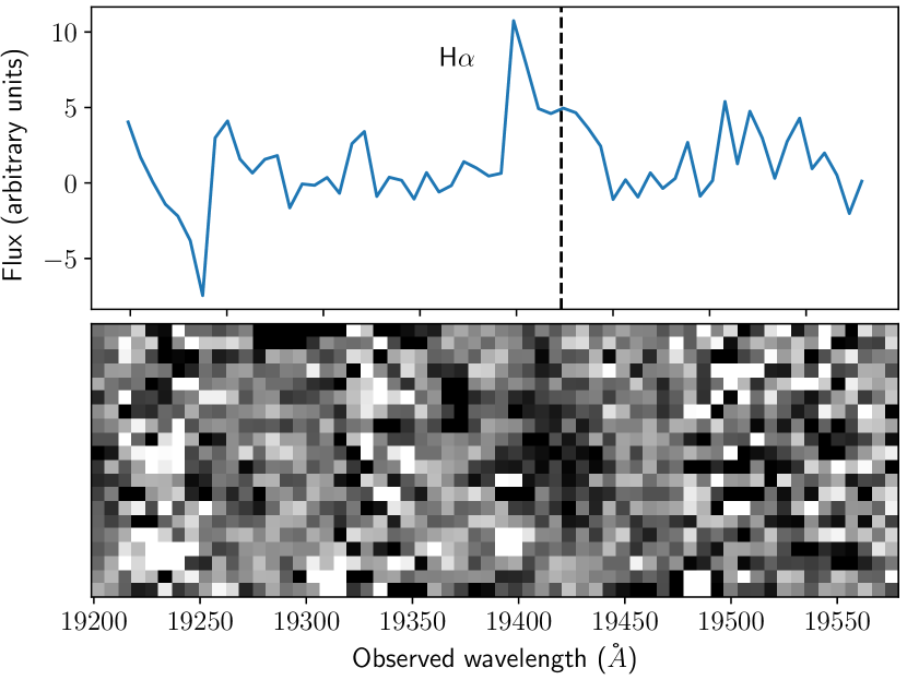
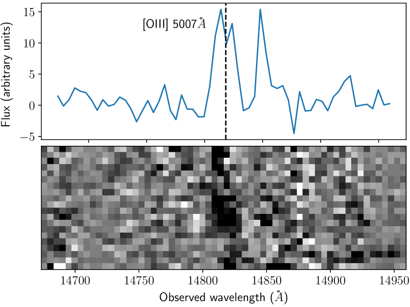
Figure 2: Top (Bottom): 2d and 1d spectrum around the H$\alpha$ ([OIII] 5007$\AA$) emission line from the counter-image to the radial arc, obtained from GNIRS observations. The 1D spectrum is extracted from a 5 pixel, corresponding to $0.75^{\prime\prime}$, aperture around each line.The secondary peak redward of [OII] visible in the 1D spectrum is due to a cosmic ray that was not properly removed in the data reduction process.

3 Multi-plane Lensing

In this work we employ multi-plane gravitational lensing, given the presence of two sources at different redshifts (corresponding to the tangential and radial arcs, respectively). We therefore briefly revisit in this section the single plane and generalized multi-plane gravitational lens formalism. In the single plane formalism a light ray of a background source is deflected by one single lens whereas, in the multi-plane case, the same light ray is deflected several times by different deflectors at different redshifts (e.g., blandford86; schneider06; gavazzi08). The lens equation of the multi-plane lens theory, which gives the relation between the angular position $\@vec{\theta}_{j}$ of a light ray in the $j$-th lens plane and the angular position in the $j=1$ plane, which is the observed image plane, is given by

$$\@vec{\theta_{j}}(\@vec{\theta}_{1})=\@vec{\theta}_{1}-\sum^{j-1}_{k=1}\frac{D_{kj}}{D_{j}}\@vec{\hat{\alpha}}(\@vec{\theta_{k}})\leavevmode\nobreak\ ,$$ (1)

where $\@vec{\theta}_{\text{N}}=\@vec{\beta}$ corresponds to the source plane if $N$ is the number of planes, $\@vec{\theta}_{k}$ is the image position on the $k$-th plane, $\@vec{\hat{\alpha}}(\@vec{\theta}_{k})$ is the deflection angle on the $k$-th plane, $D_{kj}$ is the angular diameter distance between the $k$-th and $j$-th plane, and $D_{j}$ is the angular diameter distance between us and the $j$-th plane. The total deflection angle $\@vec{\alpha}_{\text{tot}}$ is then the sum over all deflection angles on all planes

$$\@vec{\alpha}_{\text{tot}}=\sum_{k=1}^{N-1}\frac{D_{kN}}{D_{N}}\@vec{\hat{\alpha}}(\@vec{\theta}_{k})\leavevmode\nobreak\ .$$ (2)

In the case of $N=2$ the general formula reduces to the well known lens equation for the single plane formalism, namely

$$\@vec{\beta}=\@vec{\theta}-\frac{D_{\text{ds}}}{D_{\text{s}}}\@vec{\hat{\alpha}}(D_{\text{d}}\@vec{\theta})\leavevmode\nobreak\ .$$ (3)

Here the only lens is at $\@vec{\theta}=\@vec{\theta}_{1}$, the source at $\@vec{\beta}=\@vec{\theta}_{2}$, $\@vec{\hat{\alpha}}$ is the (total) deflection angle, and $D_{\text{ds}}$, $D_{\text{s}}$ and $D_{\text{d}}$ the distances between deflector (lens) and source, observer and source, and observer and deflector, respectively (e.g. schneider06).

The magnification $\mu$ is in the multi-plane formalism defined in the same way as in the single plane formalism, namely

$$\mu=\frac{1}{\det{\@vec{A}}}$$ (4)

with the Jacobian matrix

$$\@vec{A}=\frac{\partial\@vec{\beta}}{\partial\@vec{\theta}}=\frac{\partial\@vec{\theta}_{N}}{\partial\@vec{\theta}_{1}}\leavevmode\nobreak\ .$$ (5)

For the surface mass density $\Sigma(R)$ one needs the convergence $\kappa$, sometimes also called the dimensionless surface mass density. In the single-lens plane case, the convergence is

$$2\kappa=\frac{\partial\alpha_{1}}{\partial\theta_{1}}+\frac{\partial\alpha_{2}}{\partial\theta_{2}}=\@vec{\nabla}_{\theta}\cdot\@vec{\alpha}\leavevmode\nobreak\ ,$$ (6)

where $\@vec{\alpha}=(D_{\rm ds}/D_{s})\@vec{\hat{\alpha}}$. This can then be multiplied with

$$\Sigma_{\text{crit}}=\frac{c^{2}}{4\pi G}\frac{D_{\text{s}}}{D_{\text{d}}D_{\text{ds}}}$$ (7)

to derive $\Sigma(R)$ using the definition of convergence

$$\kappa=\frac{\Sigma(R)}{\Sigma_{\text{crit}}}\leavevmode\nobreak\ .$$ (8)

We can then compute the average surface mass density with the formula

$$\Sigma(<R)=\frac{\int_{0}^{R}\Sigma(R^{\prime})\leavevmode\nobreak\ 2\pi R^{\prime}\,\mathrm{d}R^{\prime}}{\pi R^{2}}\leavevmode\nobreak\ .$$ (9)

These general equations hold in the single plane case, but for the multi-plane case one defines similar, so-called effective, quantities. For calculating the effective convergence $\kappa_{\text{eff}}$ one replaces in Eq. 6 the deflection angle $\@vec{\alpha}$ with the total deflection angle $\@vec{\alpha}_{\text{tot}}$ from Eq. 2. In analogy to the case above one computes the effective average surface mass density $\Sigma_{\text{eff}}(<R)$, now using $\kappa_{\text{eff}}$ instead of $\kappa$. The consequence is that this quantity $\Sigma_{\text{eff}}(<R)$ is the gradient of the total deflection angle $\alpha_{\text{tot}}$ instead of a physical surface density.

4 Lens mass models

Since the position of an observed gravitationally lensed image depends on both baryonic and dark matter, one can use gravitational lensing as a probe for the total mass, i.e. baryonic and dark matter together. We start with a model of the lensed source positions, i.e. surface brightness peaks in the observed Einstein ring, with a single power-law plus external shear for the total mass. In addition to the main arc, which is the tangential arc, this model includes the radial arc and its counter image and is presented in Sec. 4.1. Based on this, we construct a composite mass model to describe the total mass. To disentangle the visible (baryonic) matter from the dark matter, we model the lens light distribution (see Sec. 4.2.1) which is then scaled by a constant mass-to-light ratio $M/L$, for the baryonic mass. Combining the total mass and the baryonic mass, we construct in Sec. 4.2.2 a composite mass model of baryons and dark matter assuming a power-law (barkana98), a NFW profile (navarro97), or a generalized NFW profile for the dark matter distribution. We use then a model based on the full HST images (Sec. 4.3) to refine our image positions (Sec. 4.4). In these models we always include the radial arc and our assumption for its counter image. Only in the last section with the redefined image positions we treat explicitly models with and without the radial arc as constraints. This would allow us to quantify the additional constraint on the inner dark matter distribution of the Cosmic Horseshoe from the radial arc, which is the primary goal of this paper.

For the modeling, we use Glee (Gravitational Lens Efficient Explorer), a gravitational lensing software developed by S. H. Suyu and A. Halkola (suyu10; suyu12). This software contains several types of lens and light profiles and uses Bayesian analysis such as simulated annealing and Markov Chain Monte Carlo (MCMC) to infer the parameter values of the profiles. The software also employs the Emcee package developed by ForemanMackey2013 for sampling the model parameters.

4.1 Power-law model for total mass distribution

In this section, we consider a simple power-law model for the total lens mass distribution, which has been shown by previous studies to describe well the observed tangential arc (e.g., belokurov07; dye08; quider09; bellagamba17). This will allow us to compare our model, that includes the radial arc, with previous models. We visually identify and use as constraints six sets of multiple image positions, where each set comes from a distinct source component. For modeling the lensed source positions we choose the image of the F475W band, since one can distinguish better between the different parts of the Einstein ring and since the arc is bluer than the lens galaxy. This is an indicator that the lens galaxy is fainter and therefore one can better identify multiple images in F475W. Here we use a singular power-law elliptical mass distribution (SPEMD; barkana98) with slope $\gamma^{\prime}=2g+1$ for the lens (where the convergence $\kappa(\@vec{\theta})\propto\@vec{\theta}^{\gamma^{\prime}-1})$ with an external shear. We infer the best-fit parameters of this model by minimizing

$$\chi^{2}=\sum_{j=1}^{N_{\rm pt}}\frac{\left(\@vec{\theta}_{j}^{\text{obs}}-\@vec{\theta}_{j}^{\text{pred}}\right)^{2}}{\sigma_{j}^{2}}$$ (10)

with Glee. Here $N_{\rm pt}$ is the number of data points, $\@vec{\theta}_{j}^{\text{pred}}$ the predicted and $\@vec{\theta}_{j}^{\text{obs}}$ the observed image position, with $\sigma_{j}$ the corresponding uncertainty of point $j$.

This model contains six sets of multiple images in addition to the radial arc and its counter image (see Fig. 6 with refined identifications that will be described in Sec. 4.4). This model has a $\chi^{2}$ of 12.6 for the image positions and the best-fit parameter and median values with 1-$\sigma$ uncertainties are given in Table 2. The obtained marginalized and best-fit values for the total mass model are in agreement with models from previous studies (e.g., dye08; spiniello11).

Table 2: Best-fit and marginalized parameter values for the model assuming a power-law profile plus external shear.

component	parameter	best-fit value	marginalized value
	$x\ [\arcsec]$	10.86	$10.92^{+0.05}_{-0.05}$
	$y\ [\arcsec]$	9.60	$9.61^{+0.04}_{-0.04}$
	$q$	0.76	$0.78^{+0.04}_{-0.04}$
power-law	$\theta$ [rad]	0.58	$0.51^{+0.07}_{-0.08}$
	$\theta_{\text{E}}$	8.06	$7.6^{+0.5}_{-0.5}$
	$r_{\text{c}}\ [\arcsec]$	0.01	$0.29^{+0.3}_{-0.3}$
	$\gamma^{\prime}$	1.7	$2.0^{+0.4}_{-0.2}$
shear	$\gamma_{\text{ext}}$	0.08	$0.07^{+0.02}_{-0.02}$
	$\phi_{\text{ext}}\ [\text{rad}]$	3.5	$3.2^{+0.2}_{-0.3}$

Note. The parameters $x$ and $y$ are centroid coordinates with respect to the bottom-left corner of our cutout, $q$ is the axis ratio, $\theta$ is the position angle measured counterclockwise from the $x$-axis, $\theta_{\text{E}}$ is the Einstein radius, $r_{\text{c}}$ is the core radius, $\gamma^{\prime}$ is the slope, $\gamma_{\text{ext}}$ is the external shear magnitude, and $\phi_{\text{ext}}$ is the external shear orientation. The constraints for this model are the selected multiple image systems. The best-fit model has an image position $\chi^{2}$ of 12.6.

4.2 Components for composite mass model

Since the light deflection depends on both the baryonic and the dark matter, we can construct a composite mass model. For the baryonic component, we need a model of the lens light to scale it by a mass-to-light ratio (Sec. 4.2.1). Since we do not have other information to infer the dark matter component, we fit to the data using different types of mass profiles (Sec. 4.2.2).

4.2.1 Lens light distribution for baryonic mass

To disentangle the baryonic matter from the dark matter, we need a model of the lens light distribution. For this we mask out all flux from other components such as stars and the Einstein ring in the image of the F160W filter. We then fit the parameters to the observed intensity value by minimizing the $\chi^{2}_{\text{lens}}$, which is defined as

$$\chi^{2}_{\text{lens}}=\sum_{j=1}^{N_{\rm p}}\frac{\left(I^{\text{obs}}_{j}-\text{PSF}\otimes I^{\text{sersic}}_{j}\right)^{2}}{\sigma_{\text{tot},j}^{2}}\leavevmode\nobreak\ .$$ (11)

Here $N_{\text{p}}$ is the number of pixels, $\sigma_{\text{tot},j}$ the total noise, i.e. background and Poisson noise (see below for details), of pixel $j$, and $\otimes$ represents the convolution of the point spread function (PSF) and the predicted intensity. It is necessary to take the convolution with the PSF into account due to telescope effects. Here we use a normalized bright star $\approx 40\arcsec$ S-W of the Cosmic Horseshoe lens as the PSF. We subtract also from the PSF a constant to counterbalance the background coming from a very bright object in the field of view which scatters light over the image.

We approximate the background noise $\sigma_{\text{bkgd}}$ as a constant that is set to the standard deviation computed from an empty region. We also include the contribution of the astrophysical Poisson noise (hasinoff12), which is expressed as a count rate for pixel $i$

$$\sigma^{2}_{\text{poisson},i}=\left(\frac{\sigma^{\prime}_{\text{tot},i}}{t_{i}}\right)^{2}=\left(\frac{\sqrt{d_{i}t_{i}}}{t_{i}}\right)^{2}=\left|\frac{d_{i}}{t_{i}}\right|\leavevmode\nobreak\ ,$$ (12)

where $t_{i}$ is the exposure time, $d_{i}$ the observed intensity of pixel $i$ (in $e^{-}$-counts per second) and $\sigma^{\prime}_{\text{tot},i}$ is the total Poisson noise (labeled with an apostrophe as it is not a rate like $\sigma_{\text{poisson,}i}$). We include the contribution of the astrophysical Poisson noise only if it is larger than the background noise. We sum the background noise and astrophysical noise in quadrature, such that $\sigma_{\text{tot},j}^{2}$ in Eq. (11) is

$$\sigma_{\text{tot},j}^{2}=\sigma_{\text{bkgd},j}^{2}+\sigma_{\text{poisson},j}^{2}\leavevmode\nobreak\ .$$ (13)

Sersic

To describe the surface brightness of the Cosmic Horseshoe lens galaxy, we use the commonly adopted Sersic profile (sersic63), which is the generalization of the de Vaucouleurs law (also called $r^{1/4}$ profile, DeVaucouleurs48). For modeling the lens light distribution we choose the observation in the F160W band, since the lens is brighter in F160W than in the other bands, and infrared bands trace better the stellar mass of the lens galaxy.

The best-fit model obtained by using two Sersic profiles and two stellar profiles (in this model we include two star-like objects, labelled object O1 and object O2 in Fig. 1) has $\chi^{2}=2.73\times 10^{4}$ (corresponding to a reduced $\chi^{2}$ of 1.74).

Chameleon

In addition to our lens light distribution model with the Sersic profile, we also model with another type of profile which mimics the Sersic profile well and allows analytic computations of lensing quantities (e.g., maller00; dutton11; suyu14). It is often called chameleon and composed by a difference of two isothermal profiles:

$$\displaystyle{\Large L(x,y)}= {\Large\frac{L_{0}}{1+q_{\text{L}}}\left(\frac{1}{\sqrt{x^{2}+y^{2}/q_{\text{L}}^{2}+4w_{\text{c}}^{2}/(1+q_{\text{L}})^{2}}}\right.}$$ (14)

$${\Large-\left.\frac{1}{\sqrt{x^{2}+y^{2}/q_{\text{L}}^{2}+4w_{\text{t}}^{2}/(1+q_{\text{L}})^{2}}}\right)\leavevmode\nobreak\ .}$$

In this equation, $q_{\text{L}}$ is the axis ratio, and $w_{\text{t}}$ and $w_{\text{c}}$ are parameters of the profile with $w_{\text{t}}>w_{\text{c}}$ to keep $L>0$.

By modeling with the chameleon profile we assume the same background noise as using the Sersic profile (see Sec. 4.2). Since the model including two isothermal profile sets and two stellar profiles for the two objects, as used above with the Sersic profile, has a $\chi^{2}$ of around two times the Sersic-$\chi^{2}$, we add a third chameleon profile and get a $\chi^{2}$ of $2.89\times 10^{4}$ which corresponds to a reduced $\chi^{2}$ of 1.85. In this model we include also objects O1, O2 and O3 (numbering follows Fig. 1), since we want to use the coordinates for the alignment of the two considered bands, F160W and F475W.

We will use both filters in the extended source modeling (see Sec. 4.3) while in the models using identified image positions we only use the F160W band for the lens light fitting. The parameter values of this best-fit model are used for the mass modeling (given in Table 3) and the corresponding image is shown in Fig. 3. The left image shows the observed intensity and the middle the modeled intensity. In the right panel one can see the normalized residuals of this model in a range ($-7\sigma,+7\sigma$). The constant gray regions are the masked-out areas (containing lensed arcs and neighbouring galaxies) in order to fit only to the flux of the lens. Although there are significant image residuals visible in the right panel, the typical baryonic mass residuals (corresponding to the light residuals scaled by $M/L$) would lead to a change in the deflection angle that is smaller than the image pixel size of $0.\arcsec 13$ at the locations of the radial arc.

In Fig. 4 we show the contributions of the different components, plotted along the $x$-axis of the cutout in units of solar luminosities for comparison of the contribution of the different light profiles. To compare those components’ widths to that of the PSF, in the same figure we show the latter (black dotted line) scaled to the lens light of the central component (plotted in red).

To convert the fitted light distribution into the baryonic mass, we assume at first a constant mass-to-light ratio. This means we scale all three light components by the same $M/L$ value. Additionally, we explore models with different $M/L$ values for the different components, either two ratios with $M/L_{\text{central}}=M/L_{\text{medium}}$ or $M/L_{\text{medium}}=M/L_{\text{outer}}$ and the remaining different, or with three different $M/L$ values one for each component. These baryonic mass models are considered in the Sections 4.3 and 4.4.1. Furthermore, since the width of the central component, shown in red in Fig 4, is comparably to the PSF’s width, and based on our modeling results in Section 4.4.1, we model in Section 6 this central component by a point mass with Einstein radius described by

$$\theta_{E,\text{point}}=\frac{4GM}{c^{2}D_{\text{d}}}$$ (15)

(where the Einstein radius is defined here for a source at redshift infinity), superseding the model that scales the central component with an $M/L$. Here $G$ is the gravitational constant, $M$ the point mass, $c$ the speed of light, and $D_{\text{d}}$ the distance to the deflector. For the remaining two components (blue and green in Fig. 4) we assume either one or two different mass-to-light ratios to scale the light to a mass.

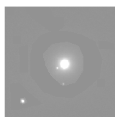
(a) observed

(b) model

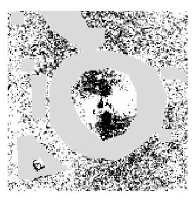
(c) normalized residuals

Figure 3: The best-fit model for the lens light distribution. The left image shows the observation of the Cosmic Horseshoe in the F160W-band, whereas the central panel shows the predicted light distribution. This model includes three chameleon profiles (see Eq. 14) and two PSF and one de Vaucouleurs profiles for the three objects. The right image shows, in a range between $-7\ \sigma$ and $+7\ \sigma$, the normalised residuals of this model. The constant gray regions are the masked-out areas (containing lensed arcs and neighboring galaxies) in order to fit only to the flux of the lens. The figures are oriented such that North is up and East is left.

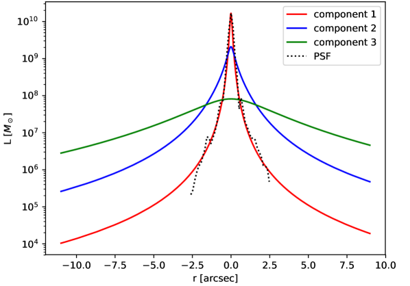
Figure 4: Different components of the chameleon profiles shown in units of solar luminosity, respectively in red (“inner”), blue (“medium”), and green (“outer” component). The total light observed from the Cosmic Horseshoe lens galaxy in the HST filter F160W is described by the sum of all three components. For comparison of the width of the components the scaled PSF is plotted with a black dotted line.

4.2.2 Dark matter halo mass distribution

In the previous section we have derived the baryonic component by modeling the light distribution. To disentangle the baryonic mass from the dark component, we model the dark matter distribution using three different profiles. At first we use a NFW (navarro97) profile but, since newer simulations predict deviations from this simple profile, we present in addition the best-fit mass model obtained assuming a power-law profile (barkana98, Singular Power-Law Elliptical Mass Distribution) (with parameters $q$ as axis ratio, $\theta_{\text{E}}$ as Einstein radius, and $r_{\text{c}}$ as core radius) and a generalized version of the NFW profile, given by

$$\rho(r)=\frac{\rho_{\text{s}}}{\left(\frac{r}{r_{\text{s}}}\right)^{\gamma_{\text{g}}}\times\left(1+\frac{r}{r_{\text{s}}}\right)^{3-\gamma_{\text{g}}}}\ ,$$ (16)

where $\gamma_{\text{g}}$ is the inner dark matter slope. The generalized NFW profile reduces to the standard NFW profile in the case $\gamma_{\text{g}}=1$.

We assume an axisymmetric lens mass distribution (axisymmetric in 3 dimensions), and impose the projected orientation of the dark matter profile to be $0^{\circ}$ or $90^{\circ}$ rotated with respect to that of the projected light distribution. We find that the $90^{\circ}$ orientation gives a better $\chi^{2}$, and thus the dark matter halo seems to be prolate, for an axisymmetric system that has its rotation axis along the minor axis of the projected light distribution. Since strong lensing is only sensitive on scales of the Einstein radius, we assume four different values for the scale radius in the NFW and gNFW profile, namely $r_{\text{s}}\equiv 18.11\arcsec$, $36.22\arcsec$, $90.54\arcsec$, and $181.08\arcsec$. These values correspond to 100 kpc, 200 kpc, 500 kpc, and 1000 kpc, respectively, for the lens redshift in the considered cosmology. We include the mass of the radial arc source in the model, using a singular isothermal sphere (SIS) profile, as this source galaxy’s mass will deflect the light coming from the background tangential arc source. The center of this profile is set to the coordinates for the radial arc source which we obtained from the multiplane lensing, calculated by the weighted mean of the mapped positions of the radial arc and its counter image on the redshift plane of the radial arc.

4.3 Extended source modeling

In the next stage of our composite mass model, we reconstruct the source surface brightness (SB) distribution and fit to the observed lensed source light, i.e. the main arc and the radial arc with its counter image. This will help us to refine our image positions afterwards. For this, we start with the mass model obtained in Sec. 4.2.2, which includes the lens light distribution described by the three chameleon profiles scaled with a constant mass-to-light ratio as baryonic mass and a power-law profile for the dark matter halo. We then allow the mass parameters to vary and, for a given set of mass parameter values, Glee reconstructs the source SB on a grid of pixels (suyu06). This source is then mapped back to the image plane to get the predicted arc. To infer the best-fit parameters, one optimizes with Glee the posterior probability distribution which is proportional to the product of the likelihood and the prior of the lens mass parameters (we refer to suyu06 and suyu10 for more details). The fitting of the SB distribution has

$$\chi_{\text{SB}}^{2}=(\@vec{d}-\@vec{d}^{\text{pred}})^{T}C_{\text{D}}^{-1}(\@vec{d}-\@vec{d}^{\text{pred}})\leavevmode\nobreak\ ,$$ (17)

where $\@vec{d}=\@vec{d}^{\text{lens}}+\@vec{d}^{\text{arc}}$ is the intensity values $d_{j}$ of pixel $j$ written as a vector with length $N_{\text{d}}$, the number of image pixels, and $C_{\text{D}}$ is the image covariance matrix. In the pixellated source SB reconstruction, we impose curvature form of regularization on the source SB pixels (suyu06).

Since we use the observed intensity of the arc to constrain our mass model and the F475W band has the brightest arc relative to the lens light, we include the F475W band in addition to the F160W which is used for the lens light model. For simplicity we assume the same structural parameters of the lens light profiles in the two bands (such as axis ratio $q$, center, and orientation $\theta$) and model only the amplitude of the three chameleon profiles and of the three objects included. Explicitly, we model the lens galaxy’s light in both filters and reconstruct the observed intensity of the Einstein ring in both. We also need to specify and model the radial arc and its counter image separately due to their different redshift from the tangential arc. This is done only in the F475W filter. The light component parameter values of this model, with a $\chi^{2}_{\rm SB}$ of $7.2\times 10^{4}$ for the F160W filter and $3.1\times 10^{5}$ for the F475W filter (the corresponding reduced $\chi^{2}_{\rm SB}$ for the total model is 1.37), are presented in Table 3. In the same table we also give the median values with 1-$\sigma$ uncertainty. The corresponding images of the best-fit model are presented in Fig. 5. In the top row one sees the images of the F160W band, in the middle row the images of the tangential arc and lens light in the F475W band, and in the bottom row the images of the radial arc in the F475W band, respectively. The images are ordered, for each row from left to right, as follows: the first image shows the observed data, the second the predicted, the third image shows the normalized residuals and the fourth image displays the reconstructed source. Despite visible residuals in the reconstruction, some of which are due to finite source pixel size, we are reproducing the global features of the tangential arcs (compare panels a to b, and e to f), to allow us to refine our multiple image positions.

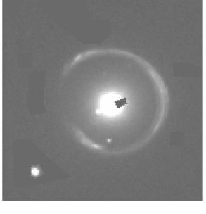
(a) observed

(b) predicted

(c) normalized residuals

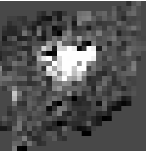
(d) source reconstruction

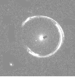
(e) observed

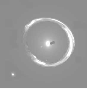
(f) predicted

(g) normalized residuals

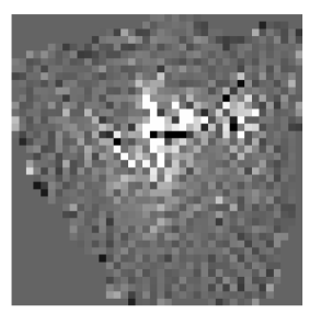
(h) source reconstruction

(i) observed

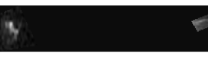
(j) predicted

(k) normalized residuals

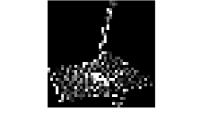
(l) source reconstruction

Figure 5: Images for the best-fit model which includes the source surface brightness reconstruction. In the top row one sees the images of the F160W band, and in the middle (tangential arc with lens) and bottom (radial arc) rows the images of the F475W band, respectively. To separate the radial arc and the tangential arc is needed since they lie at a different redshift. The images are ordered from left to right as follows: observed data, predicted model, normalized residuals in a range from $-7\sigma$ to $+7\sigma$ and the reconstructed source SB on a grid of pixels.

Table 3: Best-fit and marginalized parameter values for the lens light component of the mass model obtained by reconstructing the source surface brightness.

	Chameleon 1 (lens)		Chameleon 2 (lens)		Chameleon 3 (lens)
parameter	best-fit value	marginalized value	best-fit value	marginalized	best-fit value	marginalized
$x[\arcsec]$	11.00	$-$	11.00	$-$	11.00	$-$
$y[\arcsec]$	9.67	$-$	9.67	$-$	9.67	$-$
$q_{\text{L}}$	0.62	$0.64^{+0.02}_{-0.03}$	1.00	$1.00^{+0.00}_{-0.01}$	1.00	$1.00^{+0.00}_{-0.01}$
$\theta$[rad]	1.52	$-$	1.52	$-$	1.52	$-$
$L_{0}$ (F160W)	46.67	$-$	3.50	$-$	8.56	$-$
$w_{\text{c}}$	0.08	$0.07^{+0.01}_{-0.01}$	1.95	$2.04^{+0.06}_{-0.07}$	0.18	$0.20^{+0.03}_{-0.02}$
$w_{\text{t}}$	0.18	$0.18^{+0.01}_{-0.01}$	6.99	$7.01^{+0.03}_{-0.06}$	1.24	$1.31^{+0.02}_{-0.03}$
$L_{0}$ (F475W)	0.11	$0.11^{+0.01}_{-0.01}$	0.027	$0.029^{+0.001}_{-0.001}$	0.010	$0.010^{+0.001}_{-0.002}$

Note. This model includes three chameleon profiles (see Eq. (14)) for the F160W filter and additionally the same profiles with the same structural parameters for the F475W band. We fix the amplitudes of the F160W band since we are multiplying them with the mass-to-light ratio (variable parameter) in constructing the baryonic mass component.

We also model the Cosmic Horseshoe observation with source SB reconstruction assuming the NFW or gNFW for the dark matter halo mass. The fits give for the NFW based model a $\chi^{2}_{\rm SB}$ of $3.76\times 10^{5}$ (corresponding to a reduced $\chi^{2}_{\rm SB}=1.37$) and very similar values for the gNFW model. From this, it seems that the gNFW fits almost as well as the NFW profile. Compared with the power-law extended source model, the $\chi^{2}$ is slightly higher, but still comparable. The images reproduce the observations comparably well assuming the power-law profile, as shown in Fig. 5.

4.4 Image position modeling

Finally, we refine multiple image systems using the extended surface brightness modeling results of the last section. This time we find, similarly to what was done in Sec 4.1, eight sets of multiple images systems, in addition to the radial arc and its counter image.

4.4.1 Three chameleon profiles

If we assume a constant $M/L$ for all three chameleon profiles to scale the light to the baryonic mass, our model predicts the positions very well, with a $\chi^{2}$ of 20.23, which corresponds to a reduced $\chi^{2}$ of 1.07 (in equation 10) . Here we use the best-fit model obtained in Sec. 4.3, which adopts the power-law profile, now with core radius set to $10^{-4}$, for the dark matter distribution. This is done since the value is always very small and we want to focus on constraining the slope. Another reason is that we need to fix one parameter for our dynamics-only model which is explained more in Sec. 6. The model with the selected multiple image systems is shown in Fig. 6. The figure shows also the critical curves and caustics for both redshifts, $z_{\text{s,r}}=1.961$ and $z_{\text{s,t}}=2.381$, as well as the predicted image positions from Glee. The filled squares and circles correspond to the model source position (which is the magnification-weighted mean of the mapped source position of each image).

Figure 6: Best-fit model of the lensed source positions of the Cosmic Horseshoe, which are identified using our best-fit mass model with source SB reconstruction. This model assumes a power-law profile for the dark matter distribution. It is obtained using, as constraints, eight multiple image systems for the Einstein ring (circles) and the radial arc and its counter image (squares). We mark the predicted image positions with a cross. One can see that all predicted images are very close to the selected ones. The blue lines correspond to the critical curves (solid) and caustics (dashed) computed for the redshift of the radial arc, i.e. $z_{\text{s,r}}=1.961$, and the red line to the critical curves (solid) and caustics (dashed) computed for the redshift of the tangential arc, i.e. $z_{\text{s,t}}=2.381$. The lens position is marked with a blue star. The small additional red features near the radial arc source position, shown in the lower left corner in detail, and on the right hand side are probably due the presence of radial arc source, i.e. as a result of multi-plane lensing. Indeed, we can see that these features do not appear in the single-plane case (blue line). The filled squares and circles correspond to the weighted mean positions of the predicted source position, which are shown in more detail in the zoom in the upper/lower left corner. The figure is oriented such that North is up and East is left.

To compare how much constraints we get from the radial arc, we treat also a model based on these image positions excluding the radial arc and its counter image. Here we have to remove the SIS profile which we adopt for the radial arc source mass. With this model we get a best-fit $\chi^{2}$ of 18.87 which corresponds to a reduced $\chi^{2}$ of 1.18.

Similarly as before, we test how well we can fit the same multiple image systems, i.e. these eight sets for the tangential arc and the radial arc with its counter image as shown in Fig. 6, with our model by assuming a NFW or gNFW dark matter distribution. It turns out that our model based on the NFW profile gives a $\chi^{2}$ of 35.48 (reduced $\chi^{2}=1.87$) whereas the model based on the gNFW profile gives a $\chi^{2}$ of 35.19 (reduced $\chi^{2}=1.96$). This means that we do not fit the refined multiple image systems with the NFW or gNFW dark matter distribution as well as with the power-law. We see a big difference in $\chi^{2}$ compared to the models where we exclude the radial arc and its counter image. Explicitly, without radial arc are the $\chi^{2}$ values 25.44 (reduced $\chi^{2}=1.59$) and 25.40 (reduced $\chi^{2}=1.70$) for the NFW and gNFW profile, respectively.

While the power-law halo model fits well to the image positions, it yields a $M/L$ of around 0.4 $M_{\odot}/L_{\odot}$ that is unphysically low. On the other hand, the NFW and gNFW with a common $M/L$ for all three light components cannot fit well to the image positions, particularly those of the radial arc. Since newer publications (e.g., samurovic16; sonnenfeld18; bernardi18) predict variations in the stellar mass-to-light ratio of massive galaxies, we treat our model of the refined image position models with different mass-to-light ratios for each chameleon profile. Different ratios result in a similar effect as a radial-varying ratio. We treat this variation of different $M/L$ for all our models, that means both with and without radial arc as well as for all three different dark matter profiles NFW, gNFW and power-law. This will be considered further in Sec. 6.

4.4.2 Central point mass with constant $M/L$ of extended chameleon profiles

Since (1) we get a very small $M/L$ for the central component (compare red line in Fig. 4) in the previous model, (2) this component is very peaky that the width is smaller as the PSF width, and (3) the Cosmic Horseshoe galaxy is known to be radio active, we infer that the central component is a luminous point component like an AGN. Thus we cannot assume an $M/L$ for it to scale to the baryonic matter. Therefore we treat also models where we assume a point mass instead of the central light component. The mass range is restricted to be between $10^{8}M_{\odot}$ and $10^{10}M_{\odot}$ as these are the known limits of black hole masses (e.g., thomas16; rantala18). For the two other, extended chameleon profiles, we assume a $M/L$ to scale them to the baryonic mass. Under this assumption we are able to reproduce a good, physical meaningful model for all three adopted dark matter profiles. Since our final model will also include the kinematic information of the lens galaxy, we will discuss details only for this model in Section 6.

5 Kinematics & Dynamics

In Sec. 4 we construct a composite mass model of the Cosmic Horseshoe lens galaxy using lensing alone. In this section we present the kinematic data of the Cosmic Horseshoe lens galaxy taken from spiniello11 and a model based on dynamics-only (e.g., yildirim16; nguyen17; yildirim17; wang18).

For the dynamical modeling we use a software which was further developed by Akın Yıldırım (yildirim18) and which is based on the code from Michele Cappellari (cappellari03; cappellari08). For an overview of the Jeans ansatz and the considered parameterization, the Multi-Gaussian-Expansion (MGE) method, see Appendix LABEL:sec:dynamicstheory. We infer the best fit parameters again using Emcee as already done for the lensing part.

5.1 Lens stellar kinematic data

Following the discovery of the famous Cosmic Horseshoe by belokurov07, several follow-up observations were done. In particular, spiniello11 obtained long slit kinematic data for the lens galaxy G in March 2010. This was part of their X-Shooter program (PI: Koopmans). The observations covered a wavelength range from 300 Å to 25000 Å simultaneously with a slit centered on the galaxy, a length of 11$\arcsec$ and a width of 0.″7.

To spatially resolve the kinematic data, they defined seven apertures along the slit and summed up the signal within each aperture. The size of each aperture was chosen to be bigger than the seeing of $\approx 0.\arcsec 6$, such that independent kinematic measurement for each aperture were obtained. These data are listed in Table 4, together with the uncertainties. The obtained weighted average value of the velocity dispersion is $344\pm 25\ \text{km}\ \text{s}^{-1}$. This is within the uncertainty of the measurements. Due to the small number of available data and the huge errors we will consider the symmetrized values and uncertainties as given in Table 4.

For further details on the measurement process or the data of the stellar lens kinematics see spiniello11.

Table 4: Stellar kinematic data of the Cosmic Horseshoe lens galaxy.

Aperture distance $[\arcsec]$	$v\leavevmode\nobreak\ [\text{kms}^{-1}]$	$\sigma\leavevmode\nobreak\ [\text{km\leavevmode\nobreak\ s}^{-1}]$	$v_{\text{rm\leavevmode\nobreak\ s}}\leavevmode\nobreak\ [\text{km\leavevmode\nobreak\ s}^{-1}]$	$v_{\text{rms, sym}}\leavevmode\nobreak\ [\text{km\leavevmode\nobreak\ s}^{-1}]$
$-2.16$	$-100\pm 100$	$350\pm 100$	$364\pm 101$	$406\pm 101$
$-1.36$	$-80\pm 100$	$311\pm 76$	$321\pm 78$	$340\pm 89$
$-0.64$	$-9\pm 25$	$341\pm 26$	$341\pm 27$	$353\pm 26$
$0.00$	$0\pm 12$	$332\pm 16$	$332\pm 16$	$332\pm 16$
$+0.64$	$62\pm 18$	$360\pm 25$	$365\pm 25$	$353\pm 26$
$+1.36$	$77\pm 80$	$350\pm 100$	$358\pm 100$	$340\pm 89$
$+2.16$	$180\pm 100$	$410\pm 100$	$448\pm 101$	$406\pm 101$

Note. We give the distance along the slit measured with respect to the center, the corresponding rotation $v$ (spiniello11), the velocity dispersion $\sigma$ (spiniello11), the second velocity moments $v_{\text{rms}}$ obtained through Eq. (LABEL:eq:2moment_normal), and the symmetrized values $v_{\text{rms, sym}}$. The uncertainties $\delta v_{\text{rms}}$ is calculated through the formula $\delta v_{\text{rms}}=\sqrt{v^{2}\delta v^{2}+\sigma^{2}\delta\sigma^{2}}/v_{\text{rms}}$. The last row are the considered values in this section.

5.2 Dynamics-only modeling

Before we combine all available data to constrain maximally the mass of the Cosmic Horseshoe lens galaxy, we model the stellar kinematic data alone. We start from the best-fit model from lensing, and include the parameters anisotropy $\beta$ and inclination $i$. Since we have only seven data points (see Table 4), we can vary at most six parameters. Thus we set the core radius $r_{\text{c}}$ of the power-law, which turned out to be very small in our lensing models, to $10^{-4}$. For a correct comparison to the refined lensing models (see Sec. 4.4) we fix the core radius there too. For dynamics we will only adopt power-law and NFW dark matter distribution, i.e. no longer the generalization of the NFW profile. The reason is the small improvement compared to the NFW profile. One further reason is that otherwise we have to fix one parameter to vary fewer parameters than the available data points. In other words, for considering the generalized NFW profile we have to fix one parameter such that the number of free parameters is smaller than the number of data points. In analogy to the case of the power-law profile where we fix the core radius, we would set for the generalized NFW profile the slope $\gamma_{\text{g}}\equiv 1$. This would result in the NFW profile.

The power-law dark matter distribution gives a dynamics-only best-fit model with $\chi^{2}=0.25$. The reason why our model has a $\chi^{2}$ much smaller than 1 is due to the big uncertainties. The data points are shown in Fig. 7 (blue) with our dynamics-only model assuming power-law (solid) or NFW (dashed) dark matter distribution. Since we can easily fit to these seven data points in the given range, we treat the same model also with forecasted 5% uncertainties for every measurement. The obtained best-fit dynamics-only model has a $\chi^{2}$ of 4.95, which is clearly much higher than for the full error. The best-fit parameter and median values with 1-$\sigma$ uncertainty are given in Table 5 for the model assuming the actual measured errors. As expected, most parameters are within the 1-$\sigma$ range and the mass-to-light ratio is in a good range. The relatively large errors on the parameters are due to the small number of data points we use as constraints.

Table 5: Best-fit parameter values for our model based on the power-law dark matter distribution with dynamics-only.

component	parameter	best-fit value	marginalized
kinematics	$\beta$	0.10	$0.01^{+0.2}_{-0.3}$
	$i$	0.1	$0.1^{+0.2}_{-0.2}$
dark matter	$q$	0.82	$0.83^{+0.2}_{-0.09}$
(power-law)	$\theta_{\text{E}}$ $[\arcsec]$	2.3	$2.4^{+0.5}_{-0.4}$
	$r_{\text{c}}$ $[\arcsec]$	$\equiv 10^{-4}$	$-$
	$\gamma^{\prime}$	1.20	$1.36^{+0.4}_{-0.2}$
baryonic matter	$M/L\leavevmode\nobreak\ [M_{\odot}/L_{\odot}]$	1.8	$1.6^{+0.4}_{-0.6}$

Note. The parameters are the anisotropy $\beta$, the inclination $i$, the axis ratio $q$, the strength $\theta_{\text{E}}$, the core radius $r_{\text{c}}$, and the slope $\gamma^{\prime}$. In the last row we give the mass-to-light ratio for the baryonic component. Since we have only seven data points with huge uncertainties and vary six parameters in this model, we get also a large range of parameter values within 1-$\sigma$. The corresponding $\chi^{2}$ is 0.25. Note that we do not obtain any constraints on the anisotropy or inclination, given the assumption of a prior range of $\beta\in[-0.3,+0.3]$ and $i\in[0,+0.3]$.

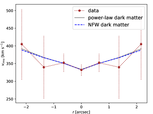
Figure 7: Values for the second velocity moments $v_{\text{rms}}$ obtained by adopting the power-law dark matter distribution (solid gray) or NFW (dashed blue) for dynamics-only. In brown are shown the measured data points with the full error bars.

For the NFW dark matter distribution we fit comparably well as with the power-law model ($\chi^{2}=0.25$ compared to $\chi^{2}=0.26$), when using the full kinematic uncertainty, while the $\chi^{2}$ is slightly higher for the reduced (forecasted 5%) uncertainty on the kinematic data ($\chi^{2}=4.95$ compared to $\chi^{2}=5.61$). Comparing power-law and the NFW, we do not find a remarkable difference, apart for the radius, which appears to be lower in the NFW forecasted case. This, however, is in agreement with the higher $\chi^{2}$ of the NFW since the predicted $v_{\text{rms}}$ values are in both versions, power-law and NFW profile, lower than the measurement. For a further detailed analysis based on dynamics-only spatially, resolved kinematic measurements would be helpful.

6 Dynamical and lensing modeling

After modeling the inner mass distribution of the Cosmic Horseshoe lens galaxy based on lensing-only (Sec. 4) and dynamics-only (Sec. 5), we now combine both approaches. In the last years huge effort has been spent to combine lensing and dynamics for strongly lensed observations to get a more robust mass model (e.g., treu02; treu04; mortlock00; gavazzi07; barnabe09; auger10; barnabe11; sonnenfeld12; grillo13; lyskova18). Since strong lensing has normally the constraints at the Einstein radius $r\approx\theta_{\text{E}}$, which is in our case $\approx 5\arcsec$, and kinematic measurements are normally in the central region around the effective radius (here $r\lesssim 2\arcsec$), one combine information at different radii with these two approaches. This will result in a better constrained model and one might break parameter degeneracies thanks to the complementary of these two approaches. However, in our particular lens system, we also use the radial arc as lensing constraints in the inner regions.

Although using the HST surface brightness observations would provide more lensing constraints, we consider here only the refined image positions presented in Sec. 4.4. The reason for this choice is that we would otherwise overwhelm the 7 data points from dynamics with more than $10^{5}$ surface brightness pixel from the images. The data points coming from the identified image positions are still higher, but at the same order of magnitude. Moreover, with this method we are able to weight the contribution of the radial arc and its counter image more.

When we combine dynamics and lensing, we consider again models with and without radial arc, each adopting power-law or NFW dark matter distribution, and all four versions with the full uncertainty of the kinematic data as well as with 5% as a forecast. Additionally, we treat all models with one single $M/L$ ratio as well as with different $M/L$ ratios as already done for lensing-only (see Sec. 4.2 for details). Based on the same arguments as for the lensing-only, we treat also models by replacing the PSF-like central component (shown in red in Fig. 4) by a point mass.

6.1 Three chameleon mass profiles

By combining lensing and dynamics we consider different composite mass model. As first, we use the lens light, which is composed by three chameleon profiles as obtained in Sec. 4.2.1, scaled by a constant mass-to-light ratio as baryonic component. Under this assumption, the best-fit has, when using a power-law dark matter mass distribution, a $\chi^{2}$ of 25.08, and, when using a NFW dark matter distribution, a $\chi^{2}$ of 71.54. The $\chi^{2}$ values reveal that the NFW is not as good at describing the observation as the power-law profile. However, assuming a power-law dark matter distribution, the $M/L$ value for scaling all three light components is around $0.1M_{\odot}/L_{\odot}$. This is unphysically low and results in a very high the dark matter fraction.

The next step to model the baryonic component is to allow different mass-to-light ratios for the different light components shown in Fig. 4. This allows us to fit remarkably better with the NFW profile, while we do not get much improvement adopting a power-law dark matter distribution. However, this method does not allow us to obtain meaningful models, as the central component needs an unphysically low $M/L$. Therefore, we infer that we cannot assume a mass-to-light ratio for the central component, irrespective of the dark matter distribution.

6.2 Point mass and two chameleon mass profiles

As noted in Sec. 4.4.2, the central component is probably associated with an AGN, since its light profile width is similar to the width of the PSF (see Fig. 4) and its $M/L$ was very low from the previous model in Sec. 6.1. Thus, assuming a mass-to-light ratio for this component would not be physically meaningful and we supersede it by a point mass in the range of a black hole mass. From our previous models and from the fact that the lens galaxy is very massive, we expect this point mass to be comparable to that of a supermassive black hole. For the two other light components we still assume the two fitted chameleon profiles scaled by a $M/L$, either the same $M/L$ for both components, or a different $M/L$ for each component. Moreover, we test the effect of relaxing the scale parameter $r_{\text{s}}$ of the NFW profile. It turn out to be very similar to the model by assuming a fixed value, as expected, such that we present only plots of the model with free $r_{\text{s}}$.

We see by comparison of the different models with the point mass that both dark matter profiles result in a similar $\chi^{2}$ value (see Table 6). Both dark matter distributions seem to fit the observation with an acceptable dark matter fraction between 60% and 70%. The corresponding plot is shown in Fig. LABEL:fig:bestfit_dynlensPoint_massfraction for the final models:

• lensing & dynamics, power-law dark matter, without radial arc

• lensing & dynamics, power-law dark matter, with radial arc

• lensing & dynamics, NFW dark matter, without radial arc

• lensing & dynamics, NFW dark matter, with radial arc

The dark matter fraction is defined here as the dark matter divided by the sum of baryonic matter from the scaled lens light and dark matter enclosed in the radius $r$. To be noted is that the point mass is not assumed to be pure baryonic matter, and thus not included in the baryonic component in the calculation. This results in the profile of dark matter fraction having a concave curve in the very central region. Including the point mass with less than $10^{10}M_{\odot}$ would shift the fraction insignificantly to lower values. The best-fit parameter values for these four models are given with the corresponding median values with $1\sigma$ uncertainties in Table 7 (adopting power-law dark matter distribution) and Table LABEL:tab:bestfit_pointNFW (adopting NFW with free scale radius $r_{\text{s}}$).

Table 6: Overview of the different final best-fit models with the point-mass component representing the innermost light component (red profile in Fig. 4).

DM profile	radial arc		one $M/L$		two $M/L$
	with	without	$\chi^{2}$	$\chi^{2}_{\text{red}}$	$\chi^{2}$	$\chi^{2}_{\text{red}}$
power-law	$\checkmark$		21.65	0.84	20.71	0.83
		$\checkmark$	19.90	0.91	19.58	0.94
NFW	$\checkmark$		20.14	0.78	19.95	0.80
		$\checkmark$	19.87	0.91	19.53	0.93

Table 7: Power-law dark matter halo model: Best-fit and marginalized parameter values for the mass model based on our image positions shown in Fig. 6 and the stellar kinematic data $v_{\text{rms, sym}}$ given in Table 4.

		with radial arc		without rad. arc
component	parameter	best-fit	marginalized	best-fit	marginalized
kinematics	$\beta$	0.00	$-0.04^{+0.2}_{-0.2}$	$-0.02$	$-0.06^{+0.4}_{-0.3}$
	$i$	0.15	$0.11^{+0.07}_{-0.08}$	0.3	$0.2^{+0.2}_{-0.2}$
	$q$	0.91	$0.91^{+0.02}_{-0.02}$	0.90	$0.91^{+0.04}_{-0.05}$
dark matter	$\theta_{\text{E}}\ [\arcsec]$	1.69	$1.66^{+0.07}_{-0.07}$	1.7	$1.7^{+0.3}_{-0.4}$
(power-law)	$r_{\text{c}}\ [\arcsec]$	$\equiv 10^{-4}$	$-$	$\equiv 10^{-4}$	$-$
	$\gamma^{\prime}$	1.28	$1.26^{+0.04}_{-0.04}$	1.26	$1.3^{+0.1}_{-0.1}$
shear	$\gamma_{\text{ext}}$	0.077	$0.076^{+0.007}_{-0.006}$	0.08	$0.07^{+0.03}_{-0.02}$
	$\phi_{\text{ext}}$	2.81	$2.80^{+0.04}_{-0.04}$	2.8	$2.8^{+0.1}_{-0.1}$
baryonic matter	$M/L\leavevmode\nobreak\ [M_{\odot}/L_{\odot}]$	1.8	$1.9^{+0.2}_{-0.1}$	1.7	$1.7^{+0.6}_{-0.7}$
	$\log(\theta_{\text{E, point}})$	$-1.01$	$-1.09^{+0.08}_{0.3}$	$-2.0$	$-2.4^{+1.3}_{-1.6}$

Note. The parameters are the anisotropy $\beta$, the inclination $i$, the axis ratio $q$, the strength $\theta_{\text{E}}$, the core radius $r_{\text{c}}$, the slope $\gamma^{\prime}$, the shear magnitude $\gamma_{\text{ext}}$, and the shear orientation $\phi_{\text{ext}}$. Additionally, we give the mass-to-light ratio $M/L$, and the strength of the point mass $\theta_{\text{E, point}}$ in logarithmic scale (i.e. $-1$ corresponds to around $10^{10}M_{\odot}$).