Reduced Basis Model Order Reduction for Navier-Stokes equations in domains with walls of varying curvature

Abstract

We consider the Navier-Stokes equations in a channel with a narrowing and walls of varying curvature. By applying the empirical interpolation method to generate an affine parameter dependency, the offline-online procedure can be used to compute reduced order solutions for parameter variations. The reduced order space is computed from the steady-state snapshot solutions by a standard POD procedure. The model is discretised with high-order spectral element ansatz functions, resulting in 4752 degrees of freedom. The proposed reduced order model produces accurate approximations of steady-state solutions for a wide range of geometries and kinematic viscosity values. The application that motivated the present study is the onset of asymmetries (i.e., symmetry breaking bifurcation) in blood flow through a regurgitant mitral valve, depending on the Reynolds number and the valve shape. Through our computational study, we found that the critical Reynolds number for the symmetry breaking increases as the wall curvature increases.

1 Introduction and Motivation

We consider the flow of an incompressible fluid through a planar channel with a narrowing, where the walls creating the narrowing have variable curvature. An application that motivated the present study is the flow of blood through a regurgitant mitral valve. Mitral regurgitation (MR) is a valvular disease characterized by abnormal leaking of blood through the mitral valve from the left ventricle into the left atrium of the heart. See Fig. 1. In certain cases, the regurgitant jet “hugs” the wall of the heart’s atrium as shown in Fig. 1 (right). These wall-hugging, non-symmetric regurgitant jets have been observed at low Reynolds numbers (Vermeulen et al. (2009); Albers et al. (2004)) and are said to undergo the Coanda effect (Wille and Fernholz (1965)). Such jets represent one of the biggest challenges in echocardiographic assessment of MR (Ginghina (2007)). In (Quaini et al. (2016); Pitton et al. (2017); Pitton and Rozza (2017); Wang et al. (2017); Hess et. al. (2018); Hess et al. (2018)), we made a connection between the cardiovascular and bioengineering literature reporting on the Coanda effect in MR and the fluid dynamics literature with the goal of identifying and understanding the main features of the corresponding flow conditions.

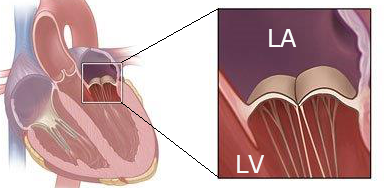
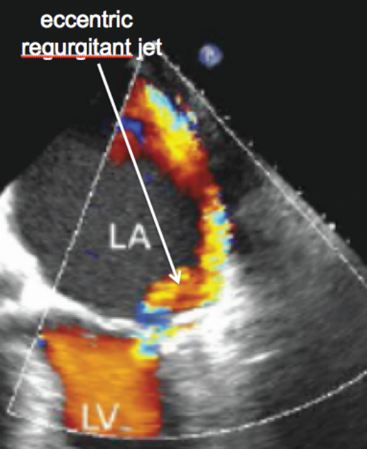
Figure 1: Left: Anatomy of the heart showing the mitral valve. Right: Echocardiographic image of a jet flowing from the left ventricle (LV) to the left atrium (LA) hugging the walls of the LA. Colors denote different fluid velocities.

In (Quaini et al. (2016); Pitton et al. (2017); Pitton and Rozza (2017); Wang et al. (2017); Hess et. al. (2018); Hess et al. (2018)), we studied what triggers the Coanda effect in a simplified setting by reformulating the problem in terms of the hydrodynamic stability of solutions of the incompressible Navier-Stokes equations in contraction-expansion channels with straight walls. Such channels have the same geometric features of MR and the wall-hugging effect is nothing but a symmetry breaking bifurcation. Here, we extend the study to contraction-expansion channels with curved walls as a first step towards more realistic geometries and eventually fluid-structure interaction.

For numerical treatment of the incompressible Navier–Stokes problem, we apply the spectral element method (SEM), which uses high-order polynomial ansatz functions such as Legendre polynomials. See, e.g., (Patera (1984); Canuto et. al. (2016, 2017)), and (Karniadakis and Sherwin (2005); Fick et al. (2018)) for applications in fluid dynamics. With a coarse partitioning of the computational domain into spectral elements, the high-order ansatz functions are prescribed over each element. The ansatz functions are modified for numerical stability and to enable continuity across element boundaries. Let $p$ be the order of the polynomial. Typically, an exponential error decay under $p$-refinement can be observed, which provides computational advantages over more standard finite element methods.

Varying wall curvature and kinematic viscosity are considered for the parametric model order reduction. From a set of sampled high-order solves, a reduced order model is generated, which approximates the high-order solutions and allows fast parameter sweeps of the two-dimensional parameter domain. The offline-online decomposition required for fast reduced order parameter evaluations is established with the empirical interpolation method (Barrault et al. (2004), Chaturantabut and Sorensen (2010), Quarteroni and Rozza (2007), Rozza (2009), Maday et.al (2015)). The reduced-order modeling (ROM) techniques described in this work are implemented in open-source project ITHACA-SEM. This extends our previous work (Hess et al. (2018), Hess and Rozza (2018)) to bifurcations in geometries with non-affine geometry variations.

The outline of the paper is as follows. In sec. 2, the model problem is defined and the parametric variations are explained. Sec. 3 provides details on the spectral element discretization and sec. 4 explains the model order reduction with the empirical interpolation. Numerical results are presented in sec. 5, while in sec. 6 conclusions are drawn and future perspectives and developments are discussed.

2 Problem Formulation

Let $\Omega\in\mathbb{R}^{2}$ be the computational domain. Incompressible, viscous fluid motion in spatial domain $\Omega$ over a time interval $(0,T)$ is governed by the incompressible Navier-Stokes equations:

$$\frac{\partial\mathbf{u}}{\partial t}+\mathbf{u}\cdot\nabla\mathbf{u} = -\nabla p+\nu\Delta\mathbf{u}+\mathbf{f},$$ (1)

$$\nabla\cdot\mathbf{u} = 0,$$ (2)

where $\mathbf{u}$ is the vector-valued velocity, $p$ is the scalar-valued pressure, $\nu$ is the kinematic viscosity and $\mathbf{f}$ is a body forcing. Boundary and initial conditions are prescribed as

$$\mathbf{u} = \mathbf{d}\quad\text{ on }\Gamma_{D}\times(0,T),$$ (3)

$$\nabla\mathbf{u}\cdot\mathbf{n} = \mathbf{g}\quad\text{ on }\Gamma_{N}\times(0,T),$$ (4)

$$\mathbf{u} = \mathbf{u}_{0}\quad\text{ in }\Omega\times 0,$$ (5)

with $\mathbf{d}$, $\mathbf{g}$ and $\mathbf{u}_{0}$ given and $\partial\Omega=\Gamma_{D}\cup\Gamma_{N}$, $\Gamma_{D}\cap\Gamma_{N}=\emptyset$. The Reynolds number $Re$, which characterizes the flow (Holmes et. al. (1996)), depends on $\nu$, a characteristic velocity $U$, and a characteristic length $L$:

$$Re=\frac{UL}{\nu}.$$ (6)

We are interested in the steady states, i.e., solutions where $\frac{\partial\mathbf{u}}{\partial t}$ vanishes. The high-order simulations are obtained through time-advancement, while the reduced order solutions are computed through fixed-point iterations.

2.1 Non-linear solver

The Oseen-iteration is a secant modulus fixed-point iteration, which in general exhibits a linear rate of convergence (Burger (2010)). It solves for a steady-state solution, i.e., $\frac{\partial\mathbf{u}}{\partial t}=0$ is assumed. Given a current iterate (or initial condition) $\mathbf{u}^{k}$, the next iterate $\mathbf{u}^{k+1}$ is found by solving the following linear system:

$$-\nu\Delta\mathbf{u}^{k+1}+(\mathbf{u}^{k}\cdot\nabla)\mathbf{u}^{k+1}+\nabla p = \mathbf{f}\text{ in }\Omega,$$

$$\nabla\cdot\mathbf{u}^{k+1} = 0\text{ in }\Omega,$$

$$\mathbf{u}^{k+1} = \mathbf{d}\text{ on }\Gamma_{D},$$

$$\nabla\mathbf{u}^{k+1}\cdot\mathbf{n} = \mathbf{g}\text{ on }\Gamma_{N}.$$

Iterations are stopped when the relative difference between iterates falls below a predefined tolerance in a suitable norm, like the $L^{2}(\Omega)$ or $H^{1}_{0}(\Omega)$ norm.

2.2 Model Description

We consider the channel flow through a narrowing created by walls of varying curvature and with variable kinematic viscosity. See Fig. 2 and 3 for the steady-state velocity components for $\nu=0.15$ in a geometry with straight walls and curved walls, respectively. In all the cases under consideration, the spectral element expansion uses modal Legendre polynomials of order $p=10$ for the velocity. The pressure ansatz space is chosen of order $p-2$ to fulfill the inf-sup stability condition (Quarteroni and Valli (1994); Boffi et. al. (2013)). A parabolic inflow profile is prescribed at the inlet (i.e., $x=0$) with horizontal velocity component $u_{x}(0,y)=y(3-y)$ for $y\in[0,3]$. At the outlet (i.e., $x=18$) we impose a stress-free boundary condition, while everywhere else a no-slip condition is prescribed. We consider symmetric boundary conditions, because we want to study the symmetry breaking due to the nonlinearity in problem (1) - (2). For a more realistic setting one would have to account for different inlet velocity profiles and the pulsatility of the flow (i.e., include the Strouhal number among the parameters).

   

   

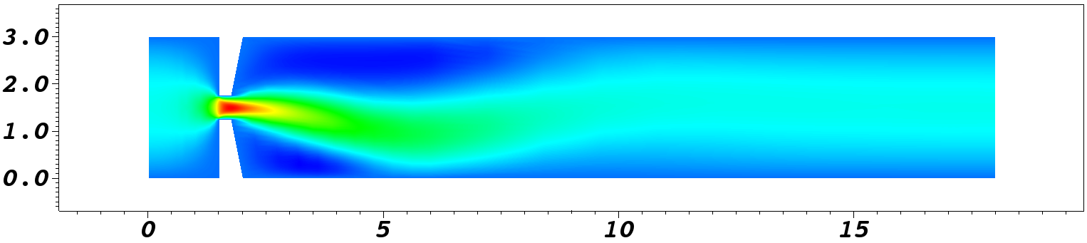
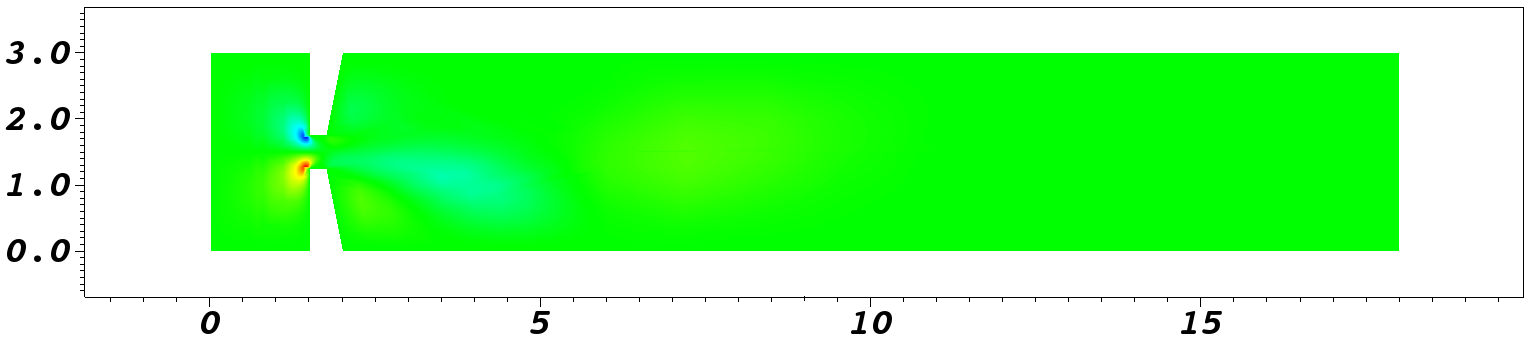
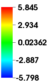
Figure 2: Full order, steady-state solution in the geometry with straight walls and for $\nu=0.15$: velocity in x-direction (top) and y-direction (bottom).

   

   

Figure 3: Full order, steady-state solution in the geometry with curved walls with the largest considered curvature and for $\nu=0.15$ : velocity in x-direction (top) and y-direction (bottom).

Each curved wall is defined by a second order polynomial, interpolating three prescribed points. While the points at the domain boundary $y=0$ and $y=3$ are kept fixed, the inner points are moved towards $x=0$ in order to create an increasing curvature. The viscosity varies in the interval $\nu\in[0.15,0.2]$. We recall that the Reynolds number $Re$ (6) depends on the kinematic viscosity. As $Re$ is varied for each fixed geometry, a supercritical pitchfork bifurcation occurs: for $Re$ higher than the critical bifurcation point, three solutions exit. Two of these solutions are stable, one with a jet towards the top wall and one with a jet towards the bottom wall, and one is unstable. The unstable solution is symmetric to the horizontal centerline at $y=1.5$, while the jet of the stable solutions is said to undergo the Coanda effect.

In this investigation, we do not deal with recovering all bifurcation branches, but limit our attention to the stable branch of solutions with jets hugging the bottom wall. However, we remark that recovering all bifurcating solutions with model reduction methods is also possible. See, e.g., (Herrero et al. (2013)).

3 Spectral Element Full Order Discretization

The spectral/hp element software framework we use for the numerical solution of problem (2) is Nektar++, version 4.4.0. The large-scale discretized system that has to be solved at each step of the Oseen-iteration can be written as

$$\begin{bmatrix}\begin{array}[]{ccc}A&-D^{T}_{bnd}&B\\ -D_{bnd}&0&-D_{int}\\ \tilde{B}^{T}&-D^{T}_{int}&C\end{array}\end{bmatrix}\begin{bmatrix}\begin{array}[]{ccc}\mathbf{v}_{bnd}\\ \mathbf{p}\\ \mathbf{v}_{int}\end{array}\end{bmatrix} =\begin{bmatrix}\begin{array}[]{ccc}\mathbf{f}_{bnd}\\ \mathbf{0}\\ \mathbf{f}_{int}\end{array}\end{bmatrix},$$ (7)

for fixed parameter vector $\boldsymbol{\mu}$, which denotes the geometrical and physical parameters. In (7), $\mathbf{v}_{bnd}$ and $\mathbf{v}_{int}$ denote the arrays of the velocity degrees of freedom on the boundary and in the interior of the domain, respectively. The array of the pressure degrees of freedom is denoted by $\mathbf{p}$. The forcing terms on the boundary and interior are $\mathbf{f}_{bnd}$ and $\mathbf{f}_{int}$, respectively. Next, we explain the matrix blocks.

Matrix $A$ assembles the boundary-boundary velocity coupling, $B$ the boundary-interior velocity coupling, $\tilde{B}$ the interior-boundary velocity coupling, and $C$ assembles the interior-interior velocity degree of freedom coupling. The matrices $D_{bnd}$ and $D_{int}$ assemble the pressure-velocity boundary and pressure-velocity interior contributions. Due to the varying geometry, each matrix is dependent on the parameter $\boldsymbol{\mu}$.

The linear system (7) is assembled in local degrees of freedom, i.e., ansatz functions with support extending over spectral element boundaries are treated seperately for each spectral element. See (Karniadakis and Sherwin (2005)) for detailed explanations. As a result, matrices $A,B,\tilde{B},C,D_{bnd}$ and $D_{int}$ have a block structure, with each block corresponding to a spectral element. This allows for an efficient matrix assembly since each spectral element is independent from the others, but the local degrees of freedom need to be gathered into the global degrees of freedom in order to obtain a non-singular system.

The boundary-boundary global element coupling is achieved with the rectangular assembly matrix $M$, which gathers the local boundary degrees of freedom. Multiplication of the first row of (7) by $M^{T}M$ sets the boundary-boundary coupling in local degrees of freedom:

$$\begin{bmatrix}\begin{array}[]{ccc}M^{T}MA&-M^{T}MD^{T}_{bnd}&M^{T}MB\\ -D_{bnd}&0&-D_{int}\\ \tilde{B}^{T}&-D^{T}_{int}&C\end{array}\end{bmatrix}\begin{bmatrix}\begin{array}[]{ccc}\mathbf{v}_{bnd}\\ \mathbf{p}\\ \mathbf{v}_{int}\end{array}\end{bmatrix} =\begin{bmatrix}\begin{array}[]{ccc}M^{T}M\mathbf{f}_{bnd}\\ \mathbf{0}\\ \mathbf{f}_{int}\end{array}\end{bmatrix}.$$ (8)

The action of the matrix in (8) on the prescribed Dirichlet boundary conditions is computed and added to the source term. Since the Dirichlet boundary conditions are known, the corresponding equations are removed from the system. Let $N_{\delta}$ denote the system size after removal of the known boundary conditions. The resulting system of high-order dimension $N_{\delta}\times N_{\delta}$ is composed of the block matrices and depends on the parameter $\boldsymbol{\mu}$. For simplicity of notation, we will write such system in compact form as:

$$\mathcal{A}(\boldsymbol{\mu})\mathbf{x}(\boldsymbol{\mu})=\mathbf{f}(\boldsymbol{\mu}).$$ (9)

4 Reduced Order Space Generation

The ROM computes an approximation to the full order model using a few modes of the POD as ansatz functions (Lassila et al. (2014)). To achieve a computational speed-up, the matrix assembly for a new parameter of interest is independent of the large-scale discretization size $N_{\delta}$. The empirical interpolation method (see sec. 4.1) computes an affine parameter dependency, which enables an offline-online decomposition (see sec. 4.2). After a time-intensive offline phase, reduced order solves can be evaluated quickly over the parameter range of interest.

The POD of $N$ (typically small) uniformly sampled full-order solves, called snapshots, is performed. The most dominant modes corresponding to $99.99\%$ of the POD energy (as suggested in Lassila et al. (2014)) form the projection matrix $U\in\mathbb{R}^{N_{\delta}\times N}$ and implicitly define the low-order space $V_{N}=\text{span}(U)$. The large-scale system (9) is then projected onto the reduced order space:

$$U^{T}\mathcal{A}(\boldsymbol{\mu})U\mathbf{x}_{N}(\boldsymbol{\mu})=U^{T}\mathbf{f}(\boldsymbol{\mu}).$$ (10)

The low order solution $\mathbf{x}_{N}(\boldsymbol{\mu})$ approximates the large-scale solution as $\mathbf{x}(\boldsymbol{\mu})\approx U\mathbf{x}_{N}(\boldsymbol{\mu})$. The stability properties of the full-order model do not necessarily carry over to the reduced-order model, which can introduce instabilities. In particular, the reduced order inf-sup stability constant might approach zero for some parameter value, while the full-order inf-sup stability constant is bounded away from zero. One way to alleviate this problem is by using inf-sup supremizers (Lassila et al. (2014)) or considering space-time variational approaches (Yano and Patera (2013)).

4.1 Empirical Interpolation Method

The discrete empirical interpolation method (EIM) (Barrault et al. (2004), Chaturantabut and Sorensen (2010), Quarteroni and Rozza (2007), Rozza (2009)) computes an approximate affine parameter dependency. During the snapshot computation, the parameter-dependent matrices are collected. The matrix discrete empirical interpolation (Negri et al. (2015)) allows to decompose $\mathcal{A}(\boldsymbol{\mu})$ as follows:

$$\mathcal{A}(\boldsymbol{\mu})\approx\sum_{i=1}^{Q_{a}}\tau_{i}(\boldsymbol{\mu})A_{i},$$ (11)

where $\tau_{i}(\boldsymbol{\mu})$ are scalar parameter-dependent coefficient functions and $A_{i}$ are parameter-independent matrices. Each coefficient function $\tau_{i}(\boldsymbol{\mu})$ corresponds to a single matrix entry of $\mathcal{A}(\boldsymbol{\mu})$. Since the assembly of only a few (here $Q_{a}<30$) matrix entries can be implemented efficiently, an approximation of $\mathcal{A}(\boldsymbol{\mu})$ is readily available for each new $\boldsymbol{\mu}$. As for the projection space $U$, $99.99\%$ of the POD energy is used to approximate the system matrices from the collected matrices during snapshot computation. The EIM is preformed for each submatrix identified in (8) and the actual system matrix $\mathcal{A}(\boldsymbol{\mu})$ is then composed of the separately approximated block matrices.

4.2 Offline-Online Decomposition

The offline-online decomposition (Hesthaven et al. (2016)) enables the computational speed-up of the ROM approach in many-query scenarios. It relies on an affine parameter dependency, such that all computations depending on the high-order model size $N_{\delta}$ can be performed in a parameter-independent offline phase. Then, the input-output evaluation performed online is independent of $N_{\delta}$ and thus fast.

After applying the empirical interpolation method in the geometry parameter, the parameter dependency is cast in an affine form. Therefore, there exists an affine expansion of the system matrix $\mathcal{A}(\boldsymbol{\mu})$ in the parameter $\boldsymbol{\mu}$ given by (11). To achieve fast reduced order solves, the offline-online decomposition computes the parameter independent projections offline, which are stored as small-sized matrices of the order $N\times N$. Since in an Oseen-iteration each matrix is dependent on the previous iterate, the submatrices corresponding to each basis function are assembled and then formed online using the affine expansion computed from the EIM and a fast evaluation of a single matrix entry as required by the EIM coefficient functions $\tau_{i}$.

5 Numerical Results

Snapshot solutions are sampled over a uniform $8\times 9$ grid from the full-order model, with $8$ samples along the $\nu$ parameter direction and $9$ samples along the geometry parameter direction. The number of required snapshot computations might potentially be reduced when using a greedy sampling, which requires error indicators or error estimators. See Hesthaven et al. (2016). Error estimation does even allow a certification of the ROM accuracy, but it requires an estimation of the inf-sup constant as well as a bound on the empirical interpolation error.

The vertical velocity at the point $(2,1.5)$ is used to generate the bifurcation diagram reported in Fig. 4. As expected, in a fixed geometry the symmetry breaking bifurcation occurs when the $Re$ exceeds a critical value. It is very interesting to observe that such critical value increases as the wall curvature increases, i.e. as the walls get more curved, the stronger the inertial forces need to be to break the symmetry of the solution. This means that the estimates for the critical $Re$ in 3D geometries with straight walls found in Pitton et al. (2017); Wang et al. (2017) provide a lower bound for the critical $Re$ at which the Coanda effect is observed in vivo (see Fig. 1 (right)).

We remark that the 2D case can be seen as a limit of the 3D case for channel depth tending to infinity. In Pitton et al. (2017), the influence of the channel depth on the flow pattern is investigated. It is shown that non-symmetry jets appear at higher $Re$ as the channel depth gets smaller. Thus, we expect that the critical $Re$ for the symmetry breaking in a 3D channel with curved walls to be higher than the values reported here for a 2D channel. This indicates the Coanda effect occurs in mitral valves with elongated orifices (corresponding to deeper channels).

Figure 4: Bifurcation diagram of the full order model over a uniform $8\times 9$ grid.

The accuracy of the ROM is assessed using $N=72$ snapshots for the POD to recover the original snapshot data. Fig. 5 shows the decay of the energy of the POD modes. To reach the typical threshold of $99.99\%$ on the POD energy, $N=33$ POD modes are required as RB ansatz functions.

Figure 5: Decay of POD energy of the sampled snapshot solutions.

Fig. 6 shows the bifurcation diagram of the reduced order model with $N=20$ basis functions. The absolute error at the point value is less than $0.01$ at $46$ parameter locations and less than $0.1$ at $63$ parameter locations. This indicates, that the high-order solutions have been well-resolved at these configurations. There are a few outliers, where the iteration scheme did not converge and the value for the last iterate is shown. Most likely this can be resolved by taking a finer snapshot sampling into account or by using a localized reduced-order modeling approach (Hess et. al. (2018)).

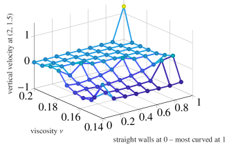
Figure 6: Bifurcation diagram of the reduced order model with reduced model size $20$.

The empirical interpolation method relies on the fast computation of a few matrix entries during the online phase. Since the spectral element ansatz functions have support over a whole spectral element, this operation cannot be performed as fast as with a finite element or finite volume method for instance, where ansatz functions have a local support. Nevertheless, the computational gain is significant after the affine form has been established. The time requirement for a single fixed point iteration step reduces from about $10$ s to $0.1$ s.

6 Conclusion and Outlook

We proposed a reduced order model that combines empirical interpolation method and a POD reduced basis technique to recover full-order solutions of the Navier–Stokes equations in domains with walls of varying curvature (non-affine variation). The non-linear geometry changes allow to simulate more realistic scenarios in the context of the Coanda effect in cardiology, but also require a fine sampling at the snapshot and empirical interpolation level. Since the model problem studied here undergoes a supercritical pitchfork bifurcation, introducing non-unique solutions, further numerical techniques are required to recover all bifurcation branches. The spectral element method is a suitable method for these tasks. However, the computational gain that one can expect is not as significant as in the case of methods using ansatz functions with a local support, such as the finite element method.

As a next step, we will enhance the reduced order model proposed here by using localizes bases in order to recover every solutions in the considered parameter domain with high accuracy.

References

- Albers et al. (2004) Albers, J., Nitsche, T., Boese, J., Simone, R. D., Wolf, I., Schroeder, A., Vahl, F.: Regurgitant jet evaluation using three-dimensional echocardiography and magnetic resonance. Ann. Thorac. Surg., 78 (2004), 96–102.
- Vermeulen et al. (2009) Vermeulen, M., Kaminsky, R., Smissen, B. V. D., Claessens, T., Segers, P., Verdonck, P., Ransbeeck, P. V.: In vitro flow modelling for mitral valve leakage quantification. In: Proc. 8th Int. Symp. Particle Image Velocimetry (2009), page 4.
- Ginghina (2007) Ginghina, C.: The Coanda Effect in Cardiology. Journal of Cardiovascular Medicine, 8 (2007), 411–413.
- Quaini et al. (2016) Quaini, A., Glowinski, R., Canic, S.: Symmetry breaking and preliminary results about a Hopf bifurcation for incompressible viscous flow in an expansion channel. International Journal of Computational Fluid Dynamics, 30:1 (2016), 7–19.
- Pitton et al. (2017) Pitton, G., Quaini, A., Rozza, G.: Computational Reduction Strategies for the Detection of Steady Bifurcations in Incompressible Fluid-Dynamics: Applications to Coanda Effect in Cardiology. Journal of Computational Physics, 344 (2017), 534–557.
- Wang et al. (2017) Wang, Y., Quaini, A., Canic, S., Vukicevic, M., Little, S.H.: 3D Experimental and Computational Analysis of Eccentric Mitral Regurgitant Jets in a Mock Imaging Heart Chamber”, Cardiovascular Engineering and Technology, 8:4, (2017), 419–438.
- Canuto et. al. (2016) Canuto, C., Hussaini, M.Y., Quarteroni, A., Zhang, Th.A.: Spectral Methods Fundamentals in Single Domains. In: Springer – Scientific Computation, (2006).
- Lassila et al. (2014) Lassila, T., Manzoni, A., Quarteroni, A., Rozza, G.: Model Order Reduction in Fluid Dynamics: Challenges and Perspectives. In: Reduced Order Methods for Modelling and Computational Reduction, Springer International Publishing, MS&A, Vol. 9, A. Quarteroni, G.Rozza eds. (2014), 235–273.
- Canuto et. al. (2017) Canuto, C., Hussaini, M.Y., Quarteroni, A., Zhang, Th.A.: Spectral Methods Evolution to Complex Geometries and Applications to Fluid Dynamics. In: Springer – Scientific Computation, (2007).
- Karniadakis and Sherwin (2005) Karniadakis, G., Sherwin, S. 2005. Spectral/hp Element Methods for Computational Fluid Dynamics. Oxford University Press, 2nd ed. (2005).
- Boffi et. al. (2013) Boffi, D., Brezzi F., Fortin, M. 2013. Mixed Finite Element Methods and Applications. Springer Series in Computational Mathematics.
- Hess et al. (2018) Hess, M.W., Quaini, A., Rozza, G. 2018. A Spectral Element Reduced Basis Method for Navier-Stokes Equations with Geometric Variations. ICOSAHOM 2018 conference proceeding. Submitted. ArXiv preprint 1812.11051.
- Quarteroni and Valli (1994) Quarteroni, A., Valli, A. 1994. Numerical Approximation of Partial Differential Equations. Springer-Verlag, Berlin-Heidelberg.
- Wille and Fernholz (1965) Wille, R., Fernholz, H. 1965. Report on the first European Mechanics Colloquium, on the Coanda effect. Journal of Fluid Mechanics, 23:4, 801–819.
- Burger (2010) Burger, M. 2010. Numerical Methods for Incompressible Flow. Lecture Notes, UCLA, http://citeseerx.ist.psu.edu/viewdoc/summary?doi=10.1.1.9.5470.
- Holmes et. al. (1996) Holmes, P., Lumley, J., Berkooz, G. 1996. Turbulence, Coherent Structures, Dynamical Systems and Symmetry. Cambridge University Press.
- Fick et al. (2018) Fick, L., Maday, Y., Patera A., Taddei T.: A stabilized POD model for turbulent flows over a range of Reynolds numbers: Optimal parameter sampling and constrained projection. Journal of Computational Physics, 371 (2018), 214–243.
- Patera (1984) Patera, A.T.: A Spectral Element Method for Fluid Dynamics; Laminar Flow in a Channel Expansion. Journal of Computational Physics, 54:3 (1984), 468–488.
- Herrero et al. (2013) Herrero, H., Maday, Y., Pla, F.: RB (Reduced Basis) for RB (Rayleigh–Bénard). Computer Methods in Applied Mechanics and Engineering, 261–262, (2013), 132–141.
- Barrault et al. (2004) Barrault, M., Maday, Y., Nguyen, N.C., Patera, A.T.: An ‘empirical interpolation’ method: application to efficient reduced-basis discretization of partial differential equations. Comptes Rendus Mathematique, 339:9, (2004), 667–672.
- Negri et al. (2015) Negri, F., Manzoni, A., Amsallam, D.: Efficient model reduction of parametrized systems by matrix discrete empirical interpolation. Journal of Computational Physics, 303, (2015), 431–454.
- Chaturantabut and Sorensen (2010) Chaturantabut, S., Sorensen, D.C.: Nonlinear Model Reduction via Discrete Empirical Interpolation. SIAM Journal on Scientific Computing, 32:5, (2010), 2737–2764.
- Hesthaven et al. (2016) Hesthaven, J.S., Rozza, G., Stamm, B.: Certified Reduced Basis Methods for Parametrized Partial Differential Equations. In: SpringerBriefs in Mathematics, (2016).
- Hess and Rozza (2018) Hess, M.W., Rozza, G.: A Spectral Element Reduced Basis Method in Parametric CFD. Numerical Mathematics and Advanced Applications - ENUMATH 2017, Springer, in press, ArXiv e-print 1712.06432, (2018).
- Hess et. al. (2018) Hess, M.W., Alla, A., Quaini, A., Rozza, G., Gunzburger, M.: A Localized Reduced-Order Modeling Approach for PDEs with Bifurcating Solutions. ArXiv e-print 1807.08851, (2018).
- Pitton and Rozza (2017) Pitton, G., Rozza, G.: On the Application of Reduced Basis Methods to Bifurcation Problems in Incompressible Fluid Dynamics. Journal of Scientific Computing, (2017).
- Quarteroni and Rozza (2007) Quarteroni, A., Rozza, G.: Numerical solution of parametrized Navier-Stokes equations by reduced basis methods. Numerical Methods for Partial Differential Equations, 23:4, (2007), 923–948.
- Rozza (2009) Rozza, G.: Reduced basis methods for Stokes equations in domains with non-affine parameter dependence. Computing and Visualization in Science, 12:1, (2009), 23–35.
- Maday et.al (2015) Maday, Y., Mula, O., Patera, A.T., Yano, M.: The generalized Empirical Interpolation Method: stability theory on Hilbert spaces with an application to the Stokes equation. Computational Methods in Applied Mechanics and Engineering, 287, 2015, 310–334.
- Yano and Patera (2013) Yano, M., Patera, A.T.: A space-time variational approach to hydrodynamic stability theory. Proceedings of the Royal Society, A, 469(2155): Article Number 20130036, 2013.