Revisit to electrical and thermal conductivities, Lorenz and Knudsen numbers in thermal QCD in a strong magnetic field

Abstract

We have explored how the electrical ($\sigma_{\rm el}$) and thermal ($\kappa$) conductivities in a thermal QCD medium get affected in weak-momentum anisotropies arising either due to a strong magnetic field or due to asymptotic expansion in a particular direction. This study, in turn, facilitates to understand the longevity of strong magnetic field through $\sigma_{\rm el}$, Lorenz number in Wiedemann-Franz law, and the validity of local equilibrium by the Knudsen number through $\kappa$. We calculate the conductivities by solving the relativistic Boltzmann transport equation in relaxation-time approximation, where the interactions are incorporated through the distribution function within the quasiparticle approach at finite $T$ and strong $B$. However, we also compare with the noninteracting scenario, which gives unusually large values, thus validating the quasiparticle description. We have found that both $\sigma_{\rm el}$ and $\kappa$ get enhanced in a magnetic field-driven anisotropy, but $\sigma_{\rm el}$ monotonically decreases with the temperature, opposite to the faster increase in the expansion-driven anisotropy. Whereas $\kappa$ increases very slowly with the temperature, contrary to its rapid increase in the expansion-driven anisotropy. Therefore the conductivities may distinguish the origin of anisotropies. The above findings are broadly attributed to three factors: the stretching and squeezing of the distribution function due to the momentum anisotropies generated by the strong magnetic field and asymptotic expansion, respectively, the dispersion relation and the resulting phase-space factor, the relaxation-time in the absence and presence of strong magnetic field. Thus $\sigma_{\rm el}$ extracts the time-dependence of initially produced strong magnetic field, which expectedly decays slower than in vacuum but the expansion-driven anisotropy makes the decay faster. The variation in $\kappa$ transpires that the Knudsen number ($\Omega$) decreases with the temperature, but the expansion-driven anisotropy reduces its magnitude, and the strong magnetic field-driven anisotropy raises its value but to less than one, thus the system can still be in local equilibrium in a range of temperature and magnetic field. Finally, the ratio, $\kappa/\sigma_{\rm el}$ in Wiedemann-Franz law in magnetic field-driven anisotropy increases linearly with temperature but its magnitude is smaller than in expansion-driven anisotropic medium. Thus the slope, i.e. the Lorenz number can make the distinction between the anisotropies of different origins.

Keywords: Electrical conductivity; Thermal conductivity; Lorenz number; Knudsen number; Strong magnetic field; Momentum anisotropy; Quasiparticle model.

1 Introduction

Relativistic heavy-ion experiments at RHIC and LHC create a new state of strongly interacting medium, known as quark gluon plasma (QGP) and are continuing to successfully collect the evidences in the form of dilepton and photon spectra [1, 2, 3], anomalous quarkonium suppression [4, 5, 6], elliptic flow [7, 8], jet quenching [9, 10, 11] etc. for the existence of QGP. The abovementioned predictions were made for the simplest possible phenomenological setting, i.e. fully central collisions, where the baryon number density is negligible and it is expected that due to the symmetric configuration of the collision, no strong magnetic fields are produced. But only a small portion of heavy-ion collisions are truly head-on, most collisions indeed occur with a finite impact parameter or centrality. As a result, the two highly charged ions impacting with a small offset may produce extremely large magnetic fields reaching between $m_{\pi}^{2}$ ($\simeq 10^{18}$ Gauss) at RHIC to 15 $m_{\pi}^{2}$ at LHC [12].

However, the naive (classical) estimates for the lifetime of these strong magnetic fields show that they only exist for a small fraction of the lifetime of QGP [13]. However, the charge transport properties of QGP may significantly extend their lifetime, thus the study of the transport coefficients, mainly, the electrical conductivity ($\sigma_{\rm el}$) becomes essential. Here our motivations are twofold, which complement each other: First, we wish to revisit $\sigma_{\rm el}$ in an isotropic hot QCD medium to check how long the magnetic field produced in relativistic heavy ion collision stays appreciably large, i.e., some sort of time-dependence of nascent magnetic field. However, the issue about the longevity of the magnetic field is not yet settled. So keeping the uncertainties about the exact nature of magnetic field in mind, if the external magnetic field still remains large, the transport properties of the medium can be significantly affected by the strong magnetic field. Our second motivation is to quantify the effect on electrical and thermal ($\kappa$) conductivities. Since $\sigma_{\rm{el}}$ is responsible for the production of electric current due to the Lenz’s law, its value becomes vital for the strength of chiral magnetic effect [14]. Moreover the electric field in mass asymmetric collisions has overall a preferred direction, which will eventually generate a charge asymmetric flow and the strength of the flow is given by $\sigma_{\rm{el}}$ [15]. Furthermore, $\sigma_{\rm{el}}$ is used as a vital input for many phenomenological applications in RHIC, LHC etc., such as the emission rate of soft photons [16]. The effects of magnetic fields on $\sigma_{\rm el}$ for quark matter have been investigated previously in different models, such as quenched SU($2$) lattice gauge theory [17], the dilute instanton-liquid model [18], the nonlinear electromagnetic currents [19, 20], axial Hall current [21], real-time formalism using the diagrammatic method [22], effective fugacity approach [23] etc.

In ultrarelativistic heavy ion collisions, it is observed that the suppression of charged particle production gets reduced while going from central to noncentral Pb$+$Pb collisions [24, 25], where strong magnetic field exists too. Therefore such strong magnetic field might significantly affect the production of particles especially the quarks which are produced within short time scale less than $\sim 1$ fm and can alter their dynamics too. A comprehensive studies on how the particle production gets influenced by an external strong magnetic field are nicely depicted in refs. [26, 27, 28]. The motion of quark in strong magnetic field becomes effectively one dimensional, which in turn enhances the quark-antiquark attraction and makes it favorable for pair production and the quark pairs get polarized along the direction of magnetic field [29]. As a result, one might expect that the magnetic field might affect the anisotropic flow of the particles.

As we know already that the external magnetic field modifies the dispersion relation of a charged particle ($\omega_{i,n}=\sqrt{p_{L}^{2}+2n|q_{i}B|+m_{i}^{2}}$) quantum mechanically, where the motion along the longitudinal direction ($p_{L}$) (with respect to the magnetic field direction) remains the same as for a free particle and only the motion along the transverse direction ($p_{T}$) gets quantized in terms of the Landau levels ($n$). In strong magnetic field (SMF) limit ($eB\gg T^{2}$ as well as $eB\gg m_{i}^{2}$), only the lowest Landau level (LLL) will be occupied, i.e. $p_{T}\approx 0$, and the particle can only move along the direction of the magnetic field, resulting an anisotropy in the momentum space, i.e. $p_{L}\gg p_{T}$. Thus the anisotropic parameter, $\xi$ ($\frac{\langle{\bf p}_{T}^{2}\rangle}{2\langle p_{L}^{2}\rangle}-1$) comes out to be negative and for a weak-anisotropy ($\xi<1$), the distribution function may be approximated by stretching the isotropic one along a certain direction (say, the direction of magnetic field). Thus, to know the effects of strong magnetic field on conductivities in kinetic theory approach, an introduction of anisotropy is automatically needed.

Much earlier than the former one, it was envisaged that the relativistic heavy ion collisions at the initial stage may induce a momentum anisotropy in the local rest frame of fireball, due to the asymptotic free expansion of the fireball in the beam direction compared to its transverse direction [31, 30]. Unlike the previous one, here, $p_{T}$ is greater than $p_{L}$, hence the anisotropy parameter becomes positive. Therefore, for a weak-anisotropy ($\xi<1$), the distribution of partons can be approximated by squeezing the isotropic one along a certain direction and its effects on many phenomenological and theoretical observations have already been made. For example, the leading-order dilepton and photon yields get enhanced due to the anisotropic component [32, 33, 34, 35]. Recently, one of us had observed the effect of this kind of anisotropy on the properties of heavy quarkonium bound states [36] and the electrical conductivity [37], where the heavy quarkonia are found to dissociate earlier than its counterpart in isotropic one and the electrical conductivity decreases with the increase of anisotropy. Later its relation with the shear viscosity was explored in [38]. Besides the abovementioned anisotropies, the event-by-event fluctuations of heavy ion collisions also produce the anisotropy, which plays a crucial role in understanding new phenomena such as the elliptic flow, the triangular flow [39, 40] etc. In fact, the anisotropy generated by the event-by-event fluctuations also transpires to the final anisotropic flow angles.

Now we move on to the thermal conductivity ($\kappa$), which is related to the efficiency of the heat flow or the energy dissipation in a thermal QCD medium. Our intention is to comment on the range of temperature and possibly, magnetic field, in which the assumption of local equilibrium in hydrodynamics can be validated in terms of Knudsen number ($\Omega$). The Knudsen number is the ratio of the mean free path ($\lambda$) to the characteristic length of the system, where $\lambda$ in turn is related to $\kappa$ ($\lambda=3\kappa/(vC_{V})$). Similar to the electrical conductivity, we also wish to explore the effect of strong magnetic field on the thermal conductivity by calculating it in the presence of weak-momentum anisotropy caused by the strong magnetic field. A natural question arises about whether we can distinguish the anisotropies through the transport coefficients. Knowing that, we can improve the knowledge on the transport properties of the medium. This query might be worthy of investigation.

The electronic contribution of the thermal and electrical conductivities are not completely independent, rather their ratio is equal to the product of Lorenz number ($L$) and temperature, widely known as Wiedemann-Franz law. In fact, the ratio, $\kappa/\sigma_{\rm el}$ has approximately the same value for different metals at the same temperature. But, it diverges in quasi-one-dimensional metallic phase with decreasing temperature [41], reaching a value much larger than that found in conventional metals nearer to the insulator-metal transition [42], thermally populated electron-hole plasma in graphene [43] etc. Recently, the temperature dependence of the Lorenz number was calculated for the two-flavor quark matter in NJL model [44] and for the strongly interacting QGP medium [45]. In the metallic phase, the electronic contribution to thermal conductivity is much smaller than what would be expected from the Wiedemann-Franz law, which can be explained in terms of independent propagation of charges and heat in a strongly correlated system. However, in this work we intend to observe how the ratio gets affected due to the presence of an ambient strong magnetic field, which in turn generates the anisotropy.

In this work, we have evaluated both the conductivities in kinetic theory approach, where the relativistic Boltzmann transport equation (RBTE) is employed and is solved in the relaxation-time approximation (RTA), where, as such, there is no scope to incorporate the interaction among the partons. We circumvent the problem by incorporating the interactions among partons through their dispersion relations, known as quasiparticle model (QPM), in their distribution functions. The quasiparticle masses are conveniently obtained from their respective self energies, which, in turn, depend on the temperature and the magnetic field. Thus the presence of magnetic field affects both electrical and thermal conductivities. However, as a base line, we also compute the conductivities with the current quark masses (noninteracting), which give unusually large values, thus motivating us to use the quasiparticle model.

In brief, we have observed that the electrical and thermal conductivities of the hot QCD medium get enhanced in the presence of strong magnetic field-driven anisotropy, compared to the counterparts in the expansion-driven anisotropic medium. We have also noticed that the unusually large values of conductivities in the noninteracting scenario have been circumvented in the quasiparticle model. As a corollary, the ratio, $\kappa/\sigma_{\rm el}$ in a strong magnetic field shows linear enhancement with the temperature, whose magnitude and slope are larger than in isotropic medium but smaller than in expansion-driven anisotropic medium, thus describing different Lorenz numbers ($\kappa/(\sigma_{\rm el}T)$). We have also observed that the presence of strong magnetic field makes the Knudsen number larger (but remains less than one) than its value in the (an)isotropic medium. Therefore the transport coefficients and their ratio might help to distinguish the origin of aforesaid anisotropies in a thermal medium produced at the initial stage of ultrarelativistic heavy ion collision. However, in our present attempt, we are not exploring the anisotropy produced due to the even-by-event fluctuations.

The present work is organized as follows. In section 2, we have first revisited the electrical conductivity for an isotropic thermal medium and then proceeded for the anisotropic thermal mediums due to expansion-induced and strong magnetic field-induced anisotropies with the current quark masses. Similarly in section 3 we have done the same for the thermal conductivity. The Wiedemann-Franz law and the Knudsen number are revisited in section 4 in light of the observations made in sections 2 and 3. In section 5, we have introduced the quasiparticle mass in the presence of both temperature and strong magnetic field and recomputed the results on electrical and thermal conductivities, which in turn redefined the Wiedemann-Franz law and the Knudsen number. Finally, we have concluded our results and future outlook in section 6.

2 Electrical conductivity

Transport coefficients such as electrical conductivity and thermal conductivity of a hot QCD system can be determined using different models and approaches namely relativistic Boltzmann transport equation [46, 47, 38, 48], the Chapman-Enskog approximation [49, 45], the correlator technique using Green-Kubo formula [18, 50, 51] and the lattice simulation [52, 53, 54]. However, we will employ the relativistic Boltzmann transport equation with the relaxation-time approximation to calculate the electrical conductivity for both isotropic and anisotropic hot QCD mediums in subsections 2.1 and 2.2, respectively.

2.1 Electrical conductivity for an isotropic thermal medium

When an isotropic and hot medium of quarks, antiquarks and gluons in thermal equilibrium is disturbed infinitesimally by an electric field, an electric current $J_{\mu}$ is induced and is given by

$$J_{\mu}=\sum_{i}q_{i}g_{i}\int\frac{d^{3}\rm{p}}{(2\pi)^{3}\omega_{i}}p_{\mu}[\delta f_{i}^{q}(x,p)+\delta f_{i}^{\bar{q}}(x,p)]~{},$$ (1)

where the summation is over three flavors ($u$, $d$ and $s$) and $q_{i}$, $g_{i}$ and $\delta f_{i}^{q}$ ($\delta f_{i}^{\bar{q}}$) are the electric charge, degeneracy factor and infinitesimal change in the distribution function for the quark (antiquark) of $i$th flavor, respectively. In our calculations, we will be using $\delta f_{i}^{q}=\delta f_{i}^{\bar{q}}=\delta f_{i}$, for zero chemical potential. According to Ohm’s law, the longitudinal component of the spatial part of four-current is directly proportional to the external electric field and the proportionality factor is known as the electrical conductivity,

$$\mathbf{J}=\sigma_{\rm el}\mathbf{E}~{}.$$ (2)

The infinitesimal change in quark distribution function is defined as $\delta f_{i}=f_{i}-f_{i}^{\rm iso}$, where $f_{i}^{\rm iso}$ is the equilibrium distribution function in the isotropic medium for $i$th flavor,

$$f_{i}^{\rm iso}=\frac{1}{e^{\beta\omega_{i}}+1}~{},$$ (3)

with $\omega_{i}=\sqrt{\mathbf{p}^{2}+m_{i}^{2}}$. It is possible to obtain $\delta f_{i}$ from the relativistic Boltzmann transport equation (RBTE) [55],

$$p^{\mu}\frac{\partial f_{i}(x,p)}{\partial x^{\mu}}+q_{i}F^{\rho\sigma}p_{\sigma}\frac{\partial f_{i}(x,p)}{\partial p^{\rho}}=\mathcal{C}[f_{i}(x,p)]~{},$$ (4)

where $F^{\rho\sigma}$ denotes the electromagnetic field strength tensor and the collision term, $\mathcal{C}[f_{i}(x,p)]$ in the relaxation-time approximation is given by

$$\mathcal{C}[f_{i}(x,p)]\simeq-\frac{p_{\nu}u^{\nu}}{\tau_{i}}\delta f_{i}(x,p)~{},$$ (5)

where $u^{\nu}$ is the four-velocity of fluid in the local rest frame and the relaxation-time ($\tau_{i}$) for $i$th flavor in a thermal medium is given [56] by

$$\tau_{i}=\frac{1}{5.1T\alpha_{s}^{2}\log\left(1/\alpha_{s}\right)\left[1+0.12(2N_{i}+1)\right]}~{}.$$ (6)

To see the response of electric field, we use only $\rho=i$ and $\sigma=0$ and vice versa, components of the electromagnetic field strength tensor, i.e. $F^{i0}=\mathbf{E}$ and $F^{0i}=-\mathbf{E}$ in our calculation, thus the RBTE (4) takes the following form,

$$q_{i}\mathbf{E}\cdot\mathbf{p}\frac{\partial f_{i}^{\rm iso}}{\partial p_{0}}+q_{i}p_{0}\mathbf{E}\cdot\frac{\partial f_{i}^{\rm iso}}{\partial\mathbf{p}}=-\frac{p_{0}}{\tau_{i}}\delta f_{i}~{}.$$ (7)

Hence the infinitesimal disturbance is obtained as

$$\delta f_{i}=2q_{i}\tau_{i}\beta\frac{\mathbf{E}\cdot\mathbf{p}}{\omega_{i}}f_{i}^{\rm iso}(1-f_{i}^{\rm iso})~{}.$$ (8)

Now substituting the value of $\delta f_{i}$ in eq. (1), we obtain the electrical conductivity for an isotropic thermal medium,

$$\sigma_{\rm el}^{\rm iso}=\frac{2\beta}{3\pi^{2}}\sum_{i}g_{i}q_{i}^{2}\int d{\rm p}~{}\frac{{\rm p}^{4}}{\omega_{i}^{2}}~{}\tau_{i}~{}f_{i}^{\rm iso}(1-f_{i}^{\rm iso})~{},$$ (9)

which can now be used to show how the magnetic field varies with time in the isotropic thermal conducting medium. According to electrodynamics, the magnetic field created in vacuum due to the spatial variation of the electric field, rapidly changes over time. However for a medium with substantial value of electrical conductivity, the momentary magnetic field would induce an electric current which ultimately would help to enhance the lifetime of the strong magnetic field.

2.2 Electrical conductivity for an anisotropic thermal medium

Here we will mainly discuss two types of momentum anisotropies, which may arise in the very early stages of ultrarelativistic heavy ion collisions. The first one is due to the preferential flow in the longitudinal direction compared to the transverse direction and the second one is due to the creation of a strong magnetic field. We will first revisit the former one.

2.2.1 Expansion-induced anisotropy

At early times, the QGP created in the heavy ion collisions experiences larger longitudinal expansion than the radial expansion and this develops a local momentum anisotropy. For the weak-momentum anisotropy ($\xi<1$) in a particular direction (say $\mathbf{n}$), the distribution function can be approximated from the isotropic one [57] as

$$f_{{\rm ex},i}^{\rm aniso}(\mathbf{p};T)=\frac{1}{e^{\beta\sqrt{\rm{p}^{2}+\xi(\mathbf{p}\cdot\mathbf{n})^{2}+m_{i}^{2}}}+1}~{},$$ (10)

which can be expanded in Taylor series, and up to $\mathcal{O}(\xi)$ it takes the following form,

$$f_{{\rm ex},i}^{\rm aniso}=f_{i}^{\rm iso}-\frac{\xi\beta(\mathbf{p}\cdot\mathbf{n})^{2}}{2\omega_{i}}f_{i}^{\rm iso}(1-f_{i}^{\rm iso})~{}.$$ (11)

The anisotropic parameter ($\xi$) is generically defined in terms of the transverse and longitudinal components of momentum as

$$\xi=\frac{\left\langle\mathbf{p}_{T}^{2}\right\rangle}{2\left\langle p_{L}^{2}\right\rangle}-1~{},$$ (12)

where $p_{L}=\mathbf{p}\cdot\mathbf{n}$, $\mathbf{p}_{T}=\mathbf{p}-\mathbf{n}\cdot(\mathbf{p}\cdot\mathbf{n})$, $\mathbf{p}\equiv(\rm{p}\sin\theta\cos\phi,\rm{p}\sin\theta\sin\phi,\rm{p}\cos\theta)$, $\mathbf{n}=(\sin\alpha,0,\cos\alpha)$, $\alpha$ is the angle between z-axis and direction of anisotropy, $(\mathbf{p}\cdot\mathbf{n})^{2}=\rm{p}^{2}c(\alpha,\theta,\phi)=\rm{p}^{2}(\sin^{2}\alpha\sin^{2}\theta\cos^{2}\phi+\cos^{2}\alpha\cos^{2}\theta+\sin(2\alpha)\sin\theta\cos\theta\cos\phi)$. For $p_{T}\gg p_{L}$, $\xi$ takes positive value, which explains the removal of particles with a large momentum component along the $\mathbf{n}$ direction due to the faster longitudinal expansion than the transverse expansion [30].

Now we are going to observe how the weak-momentum anisotropy affects the electrical conductivity of the thermal medium. Thus, after solving the RBTE (4) for the anisotropic distribution function, we get $\delta f_{i}$ as

$$\delta f_{i} = \frac{2\tau_{i}\beta q_{i}\mathbf{E}\cdot\mathbf{p}}{\omega_{i}}\left[f_{i}^{\rm iso}(1-f_{i}^{\rm iso})+\frac{\xi c(\alpha,\theta,\phi)}{2}\left\{-\frac{\beta\rm{p}^{2}}{\omega_{i}}f_{i}^{\rm iso}(1-f_{i}^{\rm iso})\right.\right.$$ (13)

$$\left.\left.\hskip 56.9055pt+\frac{2\beta\rm{p}^{2}}{\omega_{i}}{f_{i}^{\rm iso}}^{2}(1-f_{i}^{\rm iso})-\frac{\rm{p}^{2}}{\omega_{i}^{2}}f_{i}^{\rm iso}(1-f_{i}^{\rm iso})+f_{i}^{\rm iso}(1-f_{i}^{\rm iso})\right\}\right],$$

which is then substituted in eq. (1) to yield the expression of electrical conductivity for an expansion-driven anisotropic medium,

$$\sigma_{\rm el,ex}^{\rm aniso} = \frac{2\beta}{3\pi^{2}}\sum_{i}g_{i}q_{i}^{2}\int d{\rm p}\frac{{\rm p}^{4}}{\omega_{i}^{2}}~{}\tau_{i}~{}f_{i}^{\rm iso}(1-f_{i}^{\rm iso})-\frac{\xi\beta^{2}}{9\pi^{2}}\sum_{i}g_{i}q_{i}^{2}\int d{\rm p}\frac{{\rm p}^{6}}{\omega_{i}^{3}}~{}\tau_{i}~{}f_{i}^{\rm iso}(1-f_{i}^{\rm iso})$$ (14)

$$+\frac{2\xi\beta^{2}}{9\pi^{2}}\sum_{i}g_{i}q_{i}^{2}\int d{\rm p}\frac{{\rm p}^{6}}{\omega_{i}^{3}}~{}\tau_{i}~{}{f_{i}^{\rm iso}}^{2}(1-f_{i}^{\rm iso})-\frac{\xi\beta}{9\pi^{2}}\sum_{i}g_{i}q_{i}^{2}\int d{\rm p}\frac{{\rm p}^{6}}{\omega_{i}^{4}}~{}\tau_{i}~{}f_{i}^{\rm iso}(1-f_{i}^{\rm iso})$$

$$+\frac{\xi\beta}{9\pi^{2}}\sum_{i}g_{i}q_{i}^{2}\int d{\rm p}\frac{{\rm p}^{4}}{\omega_{i}^{2}}~{}\tau_{i}~{}f_{i}^{\rm iso}(1-f_{i}^{\rm iso})~{},$$

where the first term in R.H.S. is the electrical conductivity for an isotropic medium. So in terms of $\sigma_{\rm el}^{\rm iso}$, $\sigma_{\rm el,ex}^{\rm aniso}$ is written as

$$\sigma_{\rm el,ex}^{\rm aniso} = \sigma_{\rm el}^{\rm iso}-\xi\left[\frac{\beta^{2}}{9\pi^{2}}\sum_{i}g_{i}q_{i}^{2}\int d{\rm p}\frac{{\rm p}^{6}}{\omega_{i}^{3}}~{}\tau_{i}~{}f_{i}^{\rm iso}(1-f_{i}^{\rm iso})\left\{1-2f_{i}^{\rm iso}+\frac{1}{\beta\omega_{i}}\right\}\right.$$ (15)

$$\left.-\frac{\beta}{9\pi^{2}}\sum_{i}g_{i}q_{i}^{2}\int d{\rm p}\frac{{\rm p}^{4}}{\omega_{i}^{2}}~{}\tau_{i}~{}f_{i}^{\rm iso}(1-f_{i}^{\rm iso})\right].$$

2.2.2 Life-span of magnetic field

Earlier, people had thought that the magnetic field generated in the heavy ion collision decays instantly. However in the presence of transport coefficient such as electrical conductivity, the lifetime of magnetic field may be elongated. To reaffirm this, we are going to see the variation of magnetic field using the value of electrical conductivity that we have calculated above for both isotropic and anisotropic mediums.

Thus, for a charged particle moving in $x$-direction, a magnetic field will be produced in the perpendicular direction of the particle trajectory, say $z$-direction. According to the Maxwell’s equations, the magnetic field created along $z$-direction is expressed, as a function of time and electrical conductivity [58] for an isotropic medium as

$$e\mathbf{B}^{\rm iso}_{\rm medium}=\frac{e^{2}b\sigma_{\rm el}^{\rm iso}}{8\pi(t-x)^{2}}e^{-\frac{b^{2}\sigma_{\rm el}^{\rm iso}}{4(t-x)}}\hat{\mathbf{z}}~{}.$$ (16)

However for an anisotropic medium, the expression for $e\mathbf{B}$ is not available, so we assumed the same expression by replacing $\sigma_{\rm el}^{\rm iso}\rightarrow\sigma_{\rm el,ex}^{\rm aniso}$, at least, for weak-anisotropy,

$$e\mathbf{B}^{\rm aniso}_{\rm medium}=\frac{e^{2}b\sigma_{\rm el,ex}^{\rm aniso}}{8\pi(t-x)^{2}}e^{-\frac{b^{2}\sigma_{\rm el,ex}^{\rm aniso}}{4(t-x)}}\hat{\mathbf{z}}~{}.$$ (17)

For the sake of comparison, the magnetic field produced in vacuum [58] is given by,

$$e\mathbf{B}_{\rm vacuum}=\frac{e^{2}b\gamma}{4\pi\left\{b^{2}+\gamma^{2}(t-x)^{2}\right\}^{3/2}}\hat{\mathbf{z}}~{},$$ (18)

where $b$ and $\gamma$ denote the impact parameter and the Lorentz factor of heavy ion collision, respectively. In equations (16) and (17), the electrical conductivity is taken as a function of time through the cooling law, $T^{3}\propto{t^{-1}}$, where the initial time and the temperature are set at $0.2$ fm and $390$ MeV, respectively. From figures 1 and 2, which are plotted at $x=0$ for the centre of mass energies $200$ GeV and $2.76$ TeV, respectively, we see that the magnetic field in the isotropic conducting medium decays very slowly as compared to the vacuum. At initial time, the fluctuation of magnetic field in a thermal medium is quite high, however after certain time, it gradually stabilizes.

However, for a conducting medium in the presence of weak-momentum anisotropy ($\xi=0.6$), we have observed (from figure 3) that the lifetime of existence of a nearly stable magnetic field in the anisotropic thermal medium is slightly less than in the isotropic thermal medium, whereas at initial time, this difference in the variations of magnetic field in two mediums is less illustrious.

As we can see from figures 1, 2 and 3, the decay of magnetic field with time is very slow in conducting medium and it nearly remains strong. So, it is plausible to explore the effect of strong magnetic field through an anisotropy, created by it.

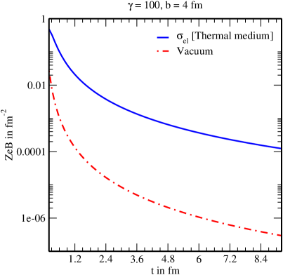
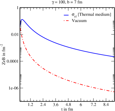
a	b

Figure 1: Comparison between the variations of magnetic field with time in an isotropic thermal conducting medium and in a vacuum for two values of the impact parameter (a) $b=4$ fm and (b) $b=7$ fm, with the Lorentz factor $\gamma=100$ for Au$+$Au collision at RHIC energy $\sqrt{s}=200$ GeV and $Z=79$ (gold nucleus).

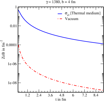
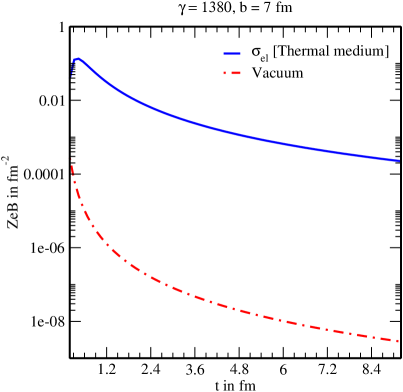
a	b

Figure 2: Comparison between the variations of magnetic field with time in an isotropic thermal conducting medium and in a vacuum for two values of the impact parameter (a) $b=4$ fm and (b) $b=7$ fm, with the Lorentz factor $\gamma=1380$ for Pb$+$Pb collision at LHC energy $\sqrt{s}=2.76$ TeV and $Z=82$ (lead nucleus).

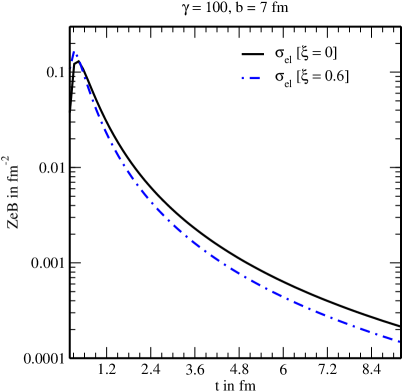
Figure 3: Comparison between the variations of magnetic field with time in isotropic and anisotropic thermal conducting mediums for impact parameter $b=7$ fm, Lorentz factor $\gamma=100$ and $Z=79$ (gold nucleus).

2.2.3 Strong magnetic field-induced anisotropy

In the presence of a magnetic field, the quark momentum $\mathbf{p}$ gets decomposed into the transverse and longitudinal components with respect to the direction of magnetic field (say, $3$-direction), hence the dispersion relation for the quark of $i$-th flavor is modified quantum mechanically into

$$\omega_{i,n}(p_{L})=\sqrt{p_{L}^{2}+m_{i}^{2}+2n\left|q_{i}B\right|}~{},$$ (19)

where $n=0$, $1$, $2$,$\cdots$ are the quantum numbers to specify the Landau levels. But in the SMF limit ($eB\gg T^{2}$), the quarks are rarely excited thermally to the higher Landau levels due to very high energy gap ($\sim\mathcal{O}(\sqrt{eB})$, hence $p_{T}$ becomes much smaller than $p_{L}$ which results in a momentum anisotropy. Thus unlike the earlier one due to the asymptotic expansion, the anisotropic parameter, $\xi$ becomes negative.

Like the earlier case, for weak anisotropy, the distribution function for quarks can be approximated from the isotropic one, except that here lower momentum particles are effectively removed from the distribution due to the negative value of $\xi$,

$$f_{{\rm B},i}^{\rm aniso}(\mathbf{p^{\prime}};T)=\frac{1}{e^{\beta\sqrt{{{\rm p}^{\prime}}^{2}+\xi(\mathbf{p^{\prime}}\cdot\mathbf{n})^{2}+m_{i}^{2}}}+1}~{}.$$ (20)

Denoting the momentum vector in strong magnetic field limit ($p_{T}=0$) by $\mathbf{p^{\prime}}=(0,0,p_{3})$ and assuming the direction of anisotropy along the direction of magnetic field, the above distribution function, for very small $\xi$, can be expanded as

$$f_{{\rm B},i}^{\rm aniso}=f_{i}^{\xi=0}-\frac{\xi\beta p_{3}^{2}}{2\omega_{i}}f_{i}^{\xi=0}(1-f_{i}^{\xi=0})~{},$$ (21)

where $\xi$-independent part of the quark distribution function in the presence of strong magnetic field is given by

$$f_{i}^{\xi=0}=\frac{1}{e^{\beta\omega_{i}}+1}~{},$$ (22)

where $\omega_{i}$ will be given from the dispersion relation (19) in SMF limit ($n=0$) after identifying $p_{L}$ with $p_{3}$, i.e. $\omega_{i}=\sqrt{p_{3}^{2}+m_{i}^{2}}$.

In the SMF limit, the quark momentum is assumed to be purely longitudinal [59, 60, 61]. Therefore when the thermal medium is disturbed infinitesimally by an electric field, an electromagnetic current is induced in the longitudinal direction (3-direction) as

$$J_{3}=\sum_{i}q_{i}g_{i}\int\frac{d^{3}\rm{p}}{(2\pi)^{3}\omega_{i}}p_{3}[\delta f_{i}^{q}(\tilde{x},\tilde{p})+\delta f_{i}^{\bar{q}}(\tilde{x},\tilde{p})]~{},$$ (23)

unlike $\mathbf{J}$ in the absence of magnetic field. In eq. (23), we have used new notations relevant to the calculations in SMF limit as $\tilde{x}=(x_{0},0,0,x_{3})$ and $\tilde{p}=(p_{0},0,0,p_{3})$. In this case, the electrical conductivity can be obtained from the third component of current in Ohm’s law,

$$J_{3}=\sigma_{\rm el}E_{3}~{}.$$ (24)

Due to dimensional reduction in the presence of a strong magnetic field, the density of states in two spatial directions perpendicular to the direction of magnetic field can be written in terms of $|q_{i}B|$ and as a result, the (integration) phase factor gets modified [62, 63] as

$$\int\frac{d^{3}{\rm p}}{(2\pi)^{3}}\rightarrow\frac{|q_{i}B|}{2\pi}\int\frac{dp_{3}}{2\pi}~{}.$$ (25)

The infinitesimal perturbation due to the action of external magnetic field is obtained from the relativistic Boltzmann transport equation in RTA, in conjunction with the strong magnetic field limit,

$$p^{0}\frac{\partial f_{i}}{\partial x^{0}}+p^{3}\frac{\partial f_{i}}{\partial x^{3}}+q_{i}F^{03}p_{3}\frac{\partial f_{i}}{\partial p^{0}}+q_{i}F^{30}p_{0}\frac{\partial f_{i}}{\partial p^{3}}=-\frac{p_{0}}{\tau^{B}_{i}}\delta f_{i}~{},$$ (26)

where $\tau^{B}_{i}$ denotes the relaxation time for quark in the presence of strong magnetic field. In the LLL approximation, the momentum-dependent relaxation-time is calculated [64] as

$$\tau^{B}_{i}=\frac{\omega_{i}\left(e^{\beta\omega_{i}}-1\right)}{\alpha_{s}C_{2}m_{i}^{2}\left(e^{\beta\omega_{i}}+1\right)}\left[1\Bigg{/}\left\{\int dp^{\prime}_{3}\frac{1}{\omega^{\prime}_{i}\left(e^{\beta\omega^{\prime}_{i}}+1\right)}\right\}\right],$$ (27)

where $C_{2}$ is the Casimir factor and the primed notations are used for antiquark. Now solving the RBTE (26) for the anisotropic distribution function, we obtain $\delta f_{i}$ as

$$\delta f_{i} = \frac{2\tau^{B}_{i}\beta q_{i}E_{3}p_{3}}{\omega_{i}}\left[f_{i}^{\xi=0}(1-f_{i}^{\xi=0})+\frac{\xi}{2}\left\{-\frac{\beta p_{3}^{2}}{\omega_{i}}f_{i}^{\xi=0}(1-f_{i}^{\xi=0})+\frac{2\beta p_{3}^{2}}{\omega_{i}}{f_{i}^{\xi=0}}^{2}(1-f_{i}^{\xi=0})\right.\right.$$ (28)

$$\left.\left.\hskip 139.41832pt-\frac{p_{3}^{2}}{\omega_{i}^{2}}f_{i}^{\xi=0}(1-f_{i}^{\xi=0})+f_{i}^{\xi=0}(1-f_{i}^{\xi=0})\right\}\right].$$

After substituting $\delta f_{i}$ in eq. (23), we get the electrical conductivity in the presence of a strong magnetic field-driven anisotropy,

$$\sigma_{\rm el,B}^{\rm aniso} = \frac{\beta}{\pi^{2}}\sum_{i}g_{i}q_{i}^{2}~{}|q_{i}B|\int dp_{3}~{}\frac{p_{3}^{2}}{\omega_{i}^{2}}~{}\tau_{i}^{B}~{}f_{i}^{\xi=0}(1-f_{i}^{\xi=0})$$ (29)

$$-\frac{\xi\beta^{2}}{2\pi^{2}}\sum_{i}g_{i}q_{i}^{2}~{}|q_{i}B|\int d{p_{3}}~{}\frac{p_{3}^{4}}{\omega_{i}^{3}}~{}\tau_{i}^{B}~{}f_{i}^{\xi=0}(1-f_{i}^{\xi=0})\left\{1-2f_{i}^{\xi=0}+\frac{1}{\beta\omega_{i}}\right\}$$

$$+\frac{\xi\beta}{2\pi^{2}}\sum_{i}g_{i}q_{i}^{2}~{}|q_{i}B|\int d{p_{3}}~{}\frac{p_{3}^{2}}{\omega_{i}^{2}}~{}\tau_{i}^{B}~{}f_{i}^{\xi=0}(1-f_{i}^{\xi=0})~{},$$

which can further be decomposed into

$$\sigma_{\rm el,B}^{\rm aniso} = \sigma_{\rm el}^{\xi=0}+\sigma_{\rm el}^{\xi\neq 0}$$ (30)

$$= \sigma_{\rm el}^{\xi=0}-\xi\left[\frac{\beta^{2}}{2\pi^{2}}\sum_{i}g_{i}q_{i}^{2}~{}|q_{i}B|\int d{p_{3}}~{}\frac{p_{3}^{4}}{\omega_{i}^{3}}~{}\tau_{i}^{B}~{}f_{i}^{\xi=0}(1-f_{i}^{\xi=0})\left\{1-2f_{i}^{\xi=0}+\frac{1}{\beta\omega_{i}}\right\}\right.$$

$$\left.-\frac{\beta}{2\pi^{2}}\sum_{i}g_{i}q_{i}^{2}~{}|q_{i}B|\int d{p_{3}}~{}\frac{p_{3}^{2}}{\omega_{i}^{2}}~{}\tau_{i}^{B}~{}f_{i}^{\xi=0}(1-f_{i}^{\xi=0})\right].$$

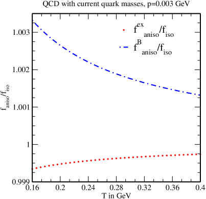
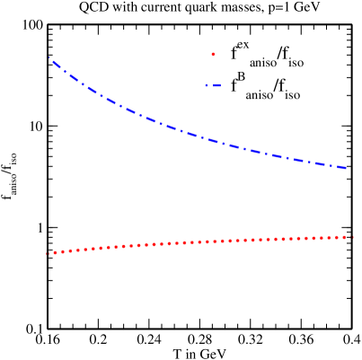
a	b

Figure 4: Variation of the ratio $f_{\rm aniso}/f_{\rm iso}$ with temperature in the presence of momentum anisotropies both due to asymptotic expansion and strong magnetic field ($15$ $m_{\pi}^{2}$) at (a) low momentum and (b) high momentum, where the current quark mass has been used.

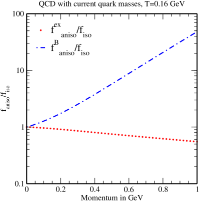
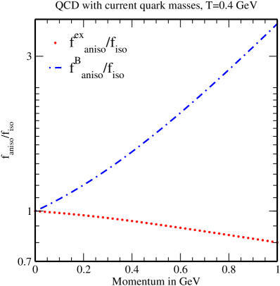
a	b

Figure 5: Variation of the ratio $f_{\rm aniso}/f_{\rm iso}$ with momentum in the presence of momentum anisotropies both due to asymptotic expansion and strong magnetic field ($15$ $m_{\pi}^{2}$) at (a) low temperature and (b) high temperature, where the current quark mass has been used.

Before analysing the results on the electrical conductivity in the presence of anisotropies arising either due to the expansion or due to the strong magnetic field, we wish to understand first how the distribution function in an isotropic medium gets affected in the presence of anisotropies, because, in kinetic theory approach, the conductivities are mainly affected by the distribution function embodying the effects of anisotropy, the phase-space factor and the relaxation time. Therefore, we must understand how the ratios, $f^{\rm ex}_{\rm aniso}/f_{\rm iso}$, $f^{\rm B}_{\rm aniso}/f_{\rm iso}$ depend on the temperature at low and high momenta or vice versa, which are numerically plotted in figures 4 and 5, respectively. The observations in the above figures can be readily understood by an order of estimate for the ratios for weak-momentum anisotropy ($\xi<1$) for nearly massless $u$ quark: $f^{\rm ex}_{\rm aniso}/f_{\rm iso}\sim e^{-c\frac{p}{T}}$, $f^{\rm B}_{\rm aniso}/f_{\rm iso}\sim e^{+c^{\prime}\frac{p}{T}}$, in both low and high momentum limits, with the constant, $c<c^{\prime}<1$. The crucial negative and positive signs in exponentials arise due to the positive and negative anisotropic parameter, in expansion-driven and magnetic field-driven cases, respectively.

Let us start with the variation of $f^{\rm ex}_{\rm aniso}/f_{\rm iso}$ with $T$ in low momentum regime (figure 4a). As $T$ increases, $p/T$ decreases, resulting an increase in $f^{\rm ex}_{\rm aniso}/f_{\rm iso}$ due to the lesser Boltzmann damping and an obvious decrease in $f^{\rm B}_{\rm aniso}/f_{\rm iso}$. The slower and relative faster variations are due to the smaller value of $c$ with respect to $c^{\prime}$. For higher momentum the variations (in figure 4b) as well as the magnitudes of the ratios are more pronounced. The variations of the ratios with momentum at a fixed temperature (in figures 5a and 5b) are much easier to understand because the variable ($p$) in the exponential is proportional to $p/T$, hence the variations become just opposite to the variation with temperature in figure 4.

Before proceeding to discuss the results, it is to be mentioned that we can not take arbitrarily large value of temperature due to the constraint of SMF limit ($eB\gg T^{2}$). For example, while computing the electrical conductivity as a function of temperature in a magnetic field-driven anisotropy with a strong magnetic field, $eB=15$ $m_{\pi}^{2}$ ($m_{\pi}^{2}\sim 0.02~{}{\rm GeV}^{2}$), the temperature can be increased from $T_{c}$ up to 0.4 GeV. If the magnetic field becomes even stronger, the temperature can go higher within the SMF limit.

The above observations on the distribution functions facilitate to understand the results on the electrical conductivity for a thermal QCD medium with three flavors ($u$, $d$ and $s$) with their current masses in figure 6. For the isotropic medium (denoted by solid line), $\sigma_{\rm el}$ increases with the temperature, whereas due to the insertion of weak-momentum anisotropy (labelled as dotted line), $\sigma_{\rm el}$ gets slightly decreased because the ratio $f^{\rm ex}_{\rm aniso}/f_{\rm iso}$ is always less than 1 for the entire range of temperature (as in figure 4a). On the other hand, the relative magnitude of $\sigma_{\rm el}$ in magnetic field-driven anisotropic medium (labelled as dashed-dotted line) becomes very large due to relatively large ratio, $f^{\rm B}_{\rm aniso}/f_{\rm iso}$. However $\sigma_{\rm el}$ increases with $T$, albeit the ratio, $f^{\rm B}_{\rm aniso}/f_{\rm iso}$ decreases with temperature (as in figure 4). The decrease in $f^{\rm B}_{\rm aniso}/f_{\rm iso}$ at high temperature becomes much slower and approaches towards unity, but the phase-space factor ($\sim|q_{i}B|$) and the relaxation time in SMF limit together compensate the minimal decrease in $f^{\rm B}_{\rm aniso}$ and give an overall increasing trend in $\sigma_{\rm el}$ in the presence of strong magnetic field. The large value of $\sigma_{\rm el}$ in the strong magnetic field regime arises due to the large relaxation-time ($\tau^{B}$), because it is inversely proportional to the square of the mass, where the current quark mass is very small. Recently, similar results have been found in [22], where $\sigma_{\rm el}$ is calculated in the diagrammatic method in the strong magnetic field regime and its large value is due to the smaller value of the current quark masses. This motivates us to recalculate the electrical conductivity with the quasiparticle masses in subsection 5.1.

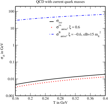
Figure 6: Variation of electrical conductivity with temperature in the presence of momentum anisotropies both due to asymptotic expansion and strong magnetic field ($15$ $m_{\pi}^{2}$), where the current quark masses have been used.

3 Thermal conductivity

This section is devoted to the determination of the thermal conductivity of a hot QCD medium using the relativistic Boltzmann transport equation. In non-relativistic case, the heat equation is obtained by the validity of the first and second laws of thermodynamics, where the flow of heat is proportional to the temperature gradient and the proportionality factor is called the thermal conductivity. The heat does not flow directly, but it diffuses, depending on the internal structure of the medium it travels through. Similarly for a relativistic QCD system, the behavior of heat flow depends on the features of the medium. Thermal conductivity of a particular medium helps to describe the heat flow in that medium and it may leave significant effects on the hydrodynamic evolution of the systems with nonzero baryon chemical potential. To see how the heat flow gets affected, we have calculated thermal conductivity for both isotropic and anisotropic hot QCD mediums in subsections 3.1 and 3.2, respectively.

3.1 Thermal conductivity for an isotropic thermal medium

Heat flow four-vector is defined as the difference between the energy diffusion and the enthalpy diffusion,

$$Q_{\mu}=\Delta_{\mu\alpha}T^{\alpha\beta}u_{\beta}-h\Delta_{\mu\alpha}N^{\alpha},$$ (31)

where $\Delta_{\mu\alpha}=g_{\mu\alpha}-u_{\mu}u_{\alpha}$ is the projection operator, $h$ is the enthalpy per particle which in terms of energy density, pressure and particle number density is represented as $h=(\varepsilon+P)/n$, $T^{\alpha\beta}$ denotes the energy-momentum tensor, and $N^{\alpha}$ is the particle flow four-vector. $N^{\alpha}$ and $T^{\alpha\beta}$ are also known as the first and second moments of the distribution function, respectively, with the following expressions,

$$N^{\alpha}=\sum_{i}2g_{i}\int\frac{d^{3}{\rm p}}{(2\pi)^{3}\omega_{i}}p^{\alpha}f_{i}(x,p)~{},$$ (32)

$$T^{\alpha\beta}=\sum_{i}2g_{i}\int\frac{d^{3}{\rm p}}{(2\pi)^{3}\omega_{i}}p^{\alpha}p^{\beta}f_{i}(x,p)~{}.$$ (33)

It is also possible to obtain the particle number density from eq. (32), the energy density and the pressure from eq. (33) as $n=N^{\alpha}u_{\alpha}$, $\varepsilon=u_{\alpha}T^{\alpha\beta}u_{\beta}$ and $P=-\Delta_{\alpha\beta}T^{\alpha\beta}/3$, respectively. From equations (31), (32) and (33), one can find that in the rest frame of the heat bath or fluid, heat flow four-vector is orthogonal to the fluid four-velocity, i.e.

$$Q_{\mu}u^{\mu}=0~{}.$$ (34)

Thus in the rest frame of the fluid, the heat flow is purely spatial and this component of heat flow due to the action of external disturbances can be written, in terms of the nonequilibrium part of the distribution function as

$$\mathbf{Q}=\sum_{i}2g_{i}\int\frac{d^{3}{\rm p}}{(2\pi)^{3}}~{}\frac{\mathbf{p}}{\omega_{i}}(\omega_{i}-h_{i})\delta f_{i}(x,p)~{}.$$ (35)

In order to define the thermal conductivity for a system, the number of particles in that system must be conserved and therefore it requires the associated chemical potential to be nonzero. In the beginning of the universe and also in the initial stages of the heavy ion collisions, the value of chemical potential ($\mu$) is small but nonzero. In the Navier-Stokes equation, the heat flow is related to the thermal potential ($U=\mu/T$) [65] as

$$Q_{\mu} = -\kappa\frac{nT^{2}}{\varepsilon+P}\nabla_{\mu}U$$ (36)

$$= \kappa\left[\nabla_{\mu}T-\frac{T}{\varepsilon+P}\nabla_{\mu}P\right],$$

where the coefficient $\kappa$ is known as the thermal conductivity and $\nabla_{\mu}=\partial_{\mu}-u_{\mu}u_{\nu}\partial^{\nu}$ is the four-gradient, which, in the rest frame of the heat bath, i.e. in the local rest frame, is replaced by $\partial_{j}$ (or $\partial/\partial x^{j}$). Thus, in the local rest frame, the spatial component of the heat flow is written as

$$\mathbf{Q}=-\kappa\left[\frac{\partial T}{\partial\mathbf{x}}-\frac{T}{nh}\frac{\partial P}{\partial\mathbf{x}}\right].$$ (37)

The thermal conductivity ($\kappa$) can be determined by comparing equations (35) and (37), so we need to first find $\delta f_{i}$. In the local rest frame, the flow velocity and temperature depend on the spatial and temporal coordinates, so the distribution function can be expanded in terms of the gradients of flow velocity and temperature. Thus, the relativistic Boltzmann transport equation (4) takes the following form,

$$p^{\mu}\partial_{\mu}T\frac{\partial f_{i}}{\partial T}+p^{\mu}\partial_{\mu}(p^{\nu}u_{\nu})\frac{\partial f_{i}}{\partial p^{0}}+q_{i}\left[F^{0j}p_{j}\frac{\partial f_{i}}{\partial p^{0}}+F^{j0}p_{0}\frac{\partial f_{i}}{\partial p^{j}}\right]=-\frac{p^{\nu}u_{\nu}}{\tau_{i}}\delta f_{i}~{},$$ (38)

where $f_{i}=f_{i}^{\rm iso}+\delta f_{i}$ and $p_{0}=\omega_{i}-\mu_{i}$, which, for very small value of $\mu_{i}$, can be approximated as $p_{0}\approx\omega_{i}$. After dropping out the infinitesimal correction to the local equilibrium distribution function ($\delta f_{i}$) from the left hand side of eq. (38) and then using the following partial derivatives,

$$\frac{\partial f_{i}^{\rm iso}}{\partial T}=\frac{p_{0}}{T^{2}}f_{i}^{\rm iso}(1-f_{i}^{\rm iso}),$$ (39)

$$\frac{\partial f_{i}^{\rm iso}}{\partial p^{0}}=-\frac{1}{T}f_{i}^{\rm iso}(1-f_{i}^{\rm iso}),$$ (40)

$$\frac{\partial f_{i}^{\rm iso}}{\partial p^{j}}=-\frac{p^{j}}{Tp_{0}}f_{i}^{\rm iso}(1-f_{i}^{\rm iso}),$$ (41)

we solve eq. (38) to get the infinitesimal disturbance,

$$\delta f_{i} = -\frac{\tau_{i}f_{i}^{\rm iso}(1-f_{i}^{\rm iso})}{p_{0}}\left[\frac{p_{0}}{T^{2}}\left\{p^{0}\partial_{0}T+p^{j}\partial_{j}T\right\}-\frac{1}{T}\left\{p^{0}\partial_{0}p_{0}+p^{j}\partial_{j}p_{0}\right\}\right.$$ (42)

$$\hskip 85.35826pt\left.-\frac{1}{T}\left\{p^{0}p^{\nu}\partial_{0}u_{\nu}+p^{j}p^{\nu}\partial_{j}u_{\nu}\right\}-\frac{2q_{i}}{T}\mathbf{E}\cdot\mathbf{p}\right]$$

$$= -\frac{\tau_{i}f_{i}^{\rm iso}(1-f_{i}^{\rm iso})}{T}\left[\frac{p_{0}}{T}\partial_{0}T+\frac{1}{T}p^{j}\partial_{j}T+T\partial_{0}\left(\frac{\mu}{T}\right)+\frac{T}{p_{0}}p^{j}\partial_{j}\left(\frac{\mu}{T}\right)\right.$$

$$\hskip 93.89418pt\left.-p^{\nu}\partial_{0}u_{\nu}-\frac{p^{j}p^{\nu}}{p_{0}}\partial_{j}u_{\nu}-\frac{2q_{i}}{p_{0}}\mathbf{E}\cdot\mathbf{p}\right].$$

Substituting $\partial_{j}\left(\frac{\mu}{T}\right)=-\frac{h}{T^{2}}\left(\partial_{j}T-\frac{T}{nh}\partial_{j}P\right)$ and using $\partial_{0}u_{\nu}=\nabla_{\nu}P/(nh)$ from the energy-momentum conservation, we get the final expression for $\delta f_{i}$ as

$$\delta f_{i} = -\frac{\tau_{i}f_{i}^{\rm iso}(1-f_{i}^{\rm iso})}{T}\left[\frac{p_{0}}{T}\partial_{0}T+\left(\frac{p_{0}-h}{p_{0}}\right)\frac{p^{j}}{T}\left(\partial_{j}T-\frac{T}{nh}\partial_{j}P\right)+T\partial_{0}\left(\frac{\mu}{T}\right)\right.$$ (43)

$$\hskip 93.89418pt\left.-\frac{p^{j}p^{\nu}}{p_{0}}\partial_{j}u_{\nu}-\frac{2q_{i}}{p_{0}}\mathbf{E}\cdot\mathbf{p}\right].$$

After substituting the $\delta f_{i}$ expression in eq. (35) and then comparing it with eq. (37), we get the thermal conductivity for the isotropic medium,

$$\kappa^{\rm iso}=\frac{\beta^{2}}{3\pi^{2}}\sum_{i}g_{i}\int d{\rm p}\frac{{\rm p}^{4}}{\omega_{i}^{2}}(\omega_{i}-h_{i})^{2}~{}\tau_{i}~{}f_{i}^{\rm iso}(1-f_{i}^{\rm iso})~{}.$$ (44)

3.2 Thermal conductivity for an anisotropic thermal medium

In this subsection we will first observe the effects due to the weak-momentum anisotropy on the thermal conductivity of hot QCD medium caused by the initial asymptotic expansion and then by the strong magnetic field as well.

3.2.1 Expansion-induced anisotropy

Using the Taylor series expansion of the anisotropic distribution function ($f^{\rm aniso}_{{\rm ex},i}$) up to the first order in $\xi$, the following partial derivatives have been calculated as

$$\frac{\partial f_{{\rm ex},i}^{\rm aniso}}{\partial T}=\frac{p_{0}f_{i}^{\rm iso}(1-f_{i}^{\rm iso})}{T^{2}}-\frac{\xi(\mathbf{p}\cdot\mathbf{n})^{2}f_{i}^{\rm iso}(1-f_{i}^{\rm iso})}{2T^{2}p_{0}}\left[\frac{p_{0}}{T}-1-\frac{2p_{0}f_{i}^{\rm iso}}{T}\right],$$ (45)

$$\frac{\partial f_{{\rm ex},i}^{\rm aniso}}{\partial p^{0}}=-\frac{f_{i}^{\rm iso}(1-f_{i}^{\rm iso})}{T}+\frac{\xi(\mathbf{p}\cdot\mathbf{n})^{2}f_{i}^{\rm iso}(1-f_{i}^{\rm iso})}{2Tp_{0}^{2}}\left[\frac{p_{0}}{T}+1-\frac{2p_{0}f_{i}^{\rm iso}}{T}\right],$$ (46)

$$\frac{\partial f_{{\rm ex},i}^{\rm aniso}}{\partial p^{j}}=-\frac{p^{j}f_{i}^{\rm iso}(1-f_{i}^{\rm iso})}{Tp_{0}}-\frac{\xi p^{j}c(\alpha,\theta,\phi)f_{i}^{\rm iso}(1-f_{i}^{\rm iso})}{2Tp_{0}}$$

$$\hskip 224.7766pt\times\left[2-\frac{{\rm p}^{2}}{p_{0}^{2}}-\frac{{\rm p}^{2}}{Tp_{0}}+\frac{2{\rm p}^{2}f_{i}^{\rm iso}}{Tp_{0}}\right],$$ (47)

which are then substituted in eq. (38) to obtain $\delta f_{i}$,

$$\delta f_{i} = -\frac{\tau_{i}f_{i}^{\rm iso}(1-f_{i}^{\rm iso})}{T}\left[1-\frac{\xi(\mathbf{p}\cdot\mathbf{n})^{2}}{2p_{0}T}+\frac{\xi(\mathbf{p}\cdot\mathbf{n})^{2}f_{i}^{\rm iso}}{p_{0}T}\right]$$ (48)

$$\times\left[\frac{p_{0}}{T}\partial_{0}T+\left(\frac{p_{0}-h_{i}}{p_{0}}\right)\frac{p^{j}}{T}\left(\partial_{j}T-\frac{T}{nh_{i}}\partial_{j}P\right)+T\partial_{0}\left(\frac{\mu}{T}\right)-\frac{p^{j}p^{\nu}}{p_{0}}\partial_{j}u_{\nu}\right]$$

$$-\frac{\tau_{i}f_{i}^{\rm iso}(1-f_{i}^{\rm iso})}{T}\frac{\xi(\mathbf{p}\cdot\mathbf{n})^{2}}{2p_{0}^{2}}\left[\frac{p_{0}}{T}\partial_{0}T+\left(\frac{p_{0}+h_{i}}{p_{0}}\right)\frac{p^{j}}{T}\left(\partial_{j}T-\frac{T}{nh_{i}}\partial_{j}P\right)-T\partial_{0}\left(\frac{\mu}{T}\right)\right.$$

$$\left.+\frac{2p^{j}}{nh_{i}}\partial_{j}P+\frac{p^{j}p^{\nu}}{p_{0}}\partial_{j}u_{\nu}\right]+\frac{2q_{i}\tau_{i}}{p_{0}T}\mathbf{E}\cdot\mathbf{p}f_{i}^{\rm iso}(1-f_{i}^{\rm iso})$$

$$\hskip 136.2885pt\times\left[1+\frac{\xi(\mathbf{p}\cdot\mathbf{n})^{2}}{2p_{0}^{2}}\left\{\frac{p_{0}^{2}}{\mathbf{p}^{2}}-1-\frac{p_{0}}{T}+\frac{2p_{0}f_{i}^{\rm iso}}{T}\right\}\right].$$

Now substituting the value of $\delta f_{i}$ in eq. (35), we find the thermal conductivity for an expansion-driven anisotropic thermal QCD medium,

$$\kappa_{\rm ex}^{\rm aniso} = \frac{\beta^{2}}{3\pi^{2}}\sum_{i}g_{i}\int d{\rm p}~{}\frac{{\rm p}^{4}}{\omega_{i}^{2}}(\omega_{i}-h_{i})^{2}~{}\tau_{i}~{}f_{i}^{\rm iso}(1-f_{i}^{\rm iso})$$ (49)

$$+\frac{\xi\beta^{2}}{18\pi^{2}}\sum_{i}g_{i}\int d{\rm p}~{}\frac{{\rm p}^{6}}{\omega_{i}^{4}}(\omega_{i}^{2}-h_{i}^{2})~{}\tau_{i}~{}f_{i}^{\rm iso}(1-f_{i}^{\rm iso})$$

$$-\frac{\xi\beta^{3}}{18\pi^{2}}\sum_{i}g_{i}\int d{\rm p}~{}\frac{{\rm p}^{6}}{\omega_{i}^{3}}(\omega_{i}-h_{i})^{2}~{}\tau_{i}~{}f_{i}^{\rm iso}(1-2f_{i}^{\rm iso})(1-f_{i}^{\rm iso})~{},$$

where the first expression in R.H.S. is the thermal conductivity for the isotropic thermal QCD medium. Thus one can write $\kappa_{\rm ex}^{\rm aniso}$ in terms of $\kappa^{\rm iso}$ as

$$\kappa_{\rm ex}^{\rm aniso} = \kappa^{\rm iso}+\xi\left[\frac{\beta^{2}}{18\pi^{2}}\sum_{i}g_{i}\int d{\rm p}~{}\frac{{\rm p}^{6}}{\omega_{i}^{4}}(\omega_{i}^{2}-h_{i}^{2})~{}\tau_{i}~{}f_{i}^{\rm iso}(1-f_{i}^{\rm iso})\right.$$ (50)

$$\left.-\frac{\beta^{3}}{18\pi^{2}}\sum_{i}g_{i}\int d{\rm p}~{}\frac{{\rm p}^{6}}{\omega_{i}^{3}}(\omega_{i}-h_{i})^{2}~{}\tau_{i}~{}f_{i}^{\rm iso}(1-2f_{i}^{\rm iso})(1-f_{i}^{\rm iso})\right].$$

We are now going to see how the thermal conductivity of the hot QCD medium gets modified due to the anisotropy developed by the strong magnetic field.

3.2.2 Strong magnetic field-induced anisotropy

The strong magnetic field restricts the dynamics of quarks to one spatial dimension, i.e. along the direction of magnetic field. So in the SMF limit, the spatial component of heat flow gets modified into

$$Q_{3}=\sum_{i}\frac{g_{i}|q_{i}B|}{2\pi^{2}}\int dp_{3}~{}\frac{p_{3}}{\omega_{i}}(\omega_{i}-h_{i}^{B})\delta f_{i}(\tilde{x},\tilde{p})~{}.$$ (51)

Similarly eq. (37) takes the following form,

$$Q_{3} = -\kappa\left[\frac{\partial T}{\partial x_{3}}-\frac{T}{nh^{B}}\frac{\partial P}{\partial x_{3}}\right]$$ (52)

$$= \kappa\left[\partial_{3}T-\frac{T}{nh^{B}}\partial_{3}P\right],$$

where $h^{B}=(\varepsilon+P)/n$ represents the enthalpy per particle in a strong magnetic field. For the charged particles in the SMF limit, the particle number density ($n$) is obtained from the following particle flow four-vector,

$$N^{\mu}=\sum_{i}\frac{g_{i}|q_{i}B|}{2\pi^{2}}\int dp_{3}\frac{\tilde{p}^{\mu}}{\omega_{i}}f_{i}(\tilde{x},\tilde{p})~{}.$$ (53)

The energy density ($\varepsilon$) and the pressure ($P$) are obtained from the following energy-momentum tensor,

$$T^{\mu\nu}=\sum_{i}\frac{g_{i}|q_{i}B|}{2\pi^{2}}\int dp_{3}\frac{\tilde{p}^{\mu}\tilde{p}^{\nu}}{\omega_{i}}f_{i}(\tilde{x},\tilde{p})~{}.$$ (54)

Now in terms of the gradients of flow velocity and temperature, the RBTE (26) in the presence of a strong magnetic field can be written as

$$\tilde{p}^{\mu}\frac{\partial T}{\partial\tilde{x}^{\mu}}\frac{\partial f_{i}}{\partial T}+\tilde{p}^{\mu}\frac{\partial(\tilde{p}^{\nu}u_{\nu})}{\partial\tilde{x}^{\mu}}\frac{\partial f_{i}}{\partial p^{0}}+q_{i}\left[F^{03}p_{3}\frac{\partial f_{i}}{\partial p^{0}}+F^{30}p_{0}\frac{\partial f_{i}}{\partial p^{3}}\right]=-\frac{\tilde{p}^{\nu}u_{\nu}}{\tau_{i}^{B}}\delta f_{i}~{},$$ (55)

where the variables, $\tilde{p}^{\mu}=(p^{0},0,0,p^{3})$ and $\tilde{x}^{\mu}=(x^{0},0,0,x^{3})$ are suited to the strong magnetic field calculation. Using the following partial derivatives,

$$\frac{\partial f_{{\rm B},i}^{\rm aniso}}{\partial T}=\frac{p_{0}f_{i}^{\xi=0}(1-f_{i}^{\xi=0})}{T^{2}}-\frac{\xi p_{3}^{2}f_{i}^{\xi=0}(1-f_{i}^{\xi=0})}{2T^{2}p_{0}}\left[\frac{p_{0}}{T}-1-\frac{2p_{0}f_{i}^{\xi=0}}{T}\right],$$ (56)

$$\frac{\partial f_{{\rm B},i}^{\rm aniso}}{\partial p^{0}}=-\frac{f_{i}^{\xi=0}(1-f_{i}^{\xi=0})}{T}+\frac{\xi p_{3}^{2}f_{i}^{\xi=0}(1-f_{i}^{\xi=0})}{2Tp_{0}^{2}}\left[\frac{p_{0}}{T}+1-\frac{2p_{0}f_{i}^{\xi=0}}{T}\right],$$ (57)

$$\frac{\partial f_{{\rm B},i}^{\rm aniso}}{\partial p^{3}}=-\frac{p^{3}f_{i}^{\xi=0}(1-f_{i}^{\xi=0})}{Tp_{0}}-\frac{\xi p^{3}f_{i}^{\xi=0}(1-f_{i}^{\xi=0})}{2Tp_{0}}$$ (58)

$$\hskip 224.7766pt\times\left[2-\frac{p_{3}^{2}}{p_{0}^{2}}-\frac{p_{3}^{2}}{Tp_{0}}+\frac{2p_{3}^{2}f_{i}^{\xi=0}}{Tp_{0}}\right],$$ (59)

we obtain $\delta f_{i}$ from eq. (55),

$$\delta f_{i} = -\frac{\tau_{i}^{B}f_{i}^{\xi=0}(1-f_{i}^{\xi=0})}{T}\left[1-\frac{\xi p_{3}^{2}}{2p_{0}T}+\frac{\xi p_{3}^{2}f_{i}^{\xi=0}}{p_{0}T}\right]$$ (60)

$$\times\left[\frac{p_{0}}{T}\partial_{0}T+\left(\frac{p_{0}-h_{i}^{B}}{p_{0}}\right)\frac{p^{3}}{T}\left(\partial_{3}T-\frac{T}{nh_{i}^{B}}\partial_{3}P\right)+T\partial_{0}\left(\frac{\mu}{T}\right)-\frac{p^{3}\tilde{p}^{\nu}}{p_{0}}\partial_{3}u_{\nu}\right]$$

$$-\frac{\tau_{i}^{B}f_{i}^{\xi=0}(1-f_{i}^{\xi=0})}{T}\frac{\xi p_{3}^{2}}{2p_{0}^{2}}\left[\frac{p_{0}}{T}\partial_{0}T+\left(\frac{p_{0}+h_{i}^{B}}{p_{0}}\right)\frac{p^{3}}{T}\left(\partial_{3}T-\frac{T}{nh_{i}^{B}}\partial_{3}P\right)-T\partial_{0}\left(\frac{\mu}{T}\right)\right.$$

$$\left.+\frac{2p^{3}}{nh_{i}^{B}}\partial_{3}P+\frac{p^{3}\tilde{p}^{\nu}}{p_{0}}\partial_{3}u_{\nu}\right]+\frac{2q_{i}\tau_{i}^{B}}{p_{0}T}E_{3}p_{3}f_{i}^{\xi=0}(1-f_{i}^{\xi=0})$$

$$\hskip 136.2885pt\times\left[1+\frac{\xi p_{3}^{2}}{2p_{0}^{2}}\left\{\frac{p_{0}^{2}}{p_{3}^{2}}-1-\frac{p_{0}}{T}+\frac{2p_{0}f_{i}^{\xi=0}}{T}\right\}\right].$$

After substituting $\delta f_{i}$ in eq. (51), the thermal conductivity in a strong magnetic field-driven anisotropic medium is obtained,

$$\kappa_{\rm B}^{\rm aniso} = \frac{\beta^{2}}{2\pi^{2}}\sum_{i}g_{i}|q_{i}B|\int dp_{3}~{}\frac{p_{3}^{2}}{\omega_{i}^{2}}(\omega_{i}-h_{i}^{B})^{2}~{}\tau_{i}^{B}~{}f_{i}^{\xi=0}(1-f_{i}^{\xi=0})$$ (61)

$$+\frac{\xi\beta^{2}}{4\pi^{2}}\sum_{i}g_{i}|q_{i}B|\int dp_{3}~{}\frac{p_{3}^{4}}{\omega_{i}^{4}}(\omega_{i}^{2}-{h_{i}^{B}}^{2})~{}\tau_{i}^{B}~{}f_{i}^{\xi=0}(1-f_{i}^{\xi=0})$$

$$-\frac{\xi\beta^{3}}{4\pi^{2}}\sum_{i}g_{i}|q_{i}B|\int dp_{3}~{}\frac{p_{3}^{4}}{\omega_{i}^{3}}(\omega_{i}-h_{i}^{B})^{2}~{}\tau_{i}^{B}~{}f_{i}^{\xi=0}(1-2f_{i}^{\xi=0})(1-f_{i}^{\xi=0})~{}.$$

Thus $\kappa_{\rm B}^{\rm aniso}$ can be rewritten in terms of $\xi$-independent and $\xi$-dependent parts as

$$\kappa_{\rm B}^{\rm aniso} = \kappa^{\xi=0}+\kappa^{\xi\neq 0}$$ (62)

$$= \kappa^{\xi=0}+\xi\left[\frac{\beta^{2}}{4\pi^{2}}\sum_{i}g_{i}|q_{i}B|\int dp_{3}~{}\frac{p_{3}^{4}}{\omega_{i}^{4}}(\omega_{i}^{2}-{h_{i}^{B}}^{2})~{}\tau_{i}^{B}~{}f_{i}^{\xi=0}(1-f_{i}^{\xi=0})\right.$$

$$\left.-\frac{\beta^{3}}{4\pi^{2}}\sum_{i}g_{i}|q_{i}B|\int dp_{3}~{}\frac{p_{3}^{4}}{\omega_{i}^{3}}(\omega_{i}-h_{i}^{B})^{2}~{}\tau_{i}^{B}~{}f_{i}^{\xi=0}(1-2f_{i}^{\xi=0})(1-f_{i}^{\xi=0})\right].$$

Figure 7 depicts how the thermal conductivity varies with temperature for the isotropic medium and for the anisotropic mediums due to expansion-driven anisotropy and strong magnetic field-driven anisotropy. We have observed that $\kappa$ for the isotropic medium increases with the temperature. Similar increasing behavior of $\kappa$ is also noticed for the expansion-driven anisotropic medium, however its magnitude becomes smaller. If the origin of anisotropy is strong magnetic field, then the magnitude of $\kappa$ becomes unusually large. The above observations on the thermal conductivity could also be attributed to the behaviors of respective distribution functions, the phase-space factor and the relaxation time, where the last two factors are severely affected by the strong magnetic field only. This again necessitates the incorporation of the interactions among quarks through the quasiparticle model.

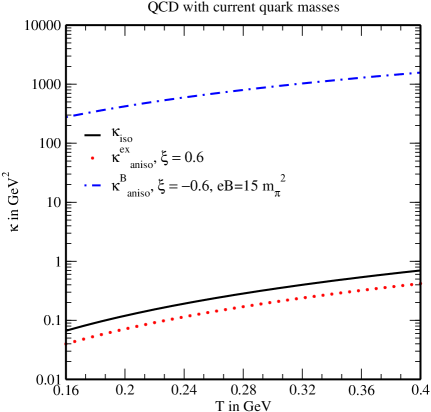
Figure 7: Variation of thermal conductivity with temperature in the presence of momentum anisotropies both due to asymptotic expansion and strong magnetic field ($15$ $m_{\pi}^{2}$), where the current quark masses have been used.

4 Applications

This section is devoted to study how the above behaviors observed in the electrical and thermal conductivities will help to understand some specific properties of the medium. In subsection 4.1, we will observe how the interplay between the conductivities through the Wiedemann-Franz law gets modified in a thermal QCD medium in the presence of anisotropies arising due to different causes. In subsection 4.2, we will calculate the Knudsen number to have a say whether the thermal QCD medium is still in local equilibrium even in the presence of different anisotropies discussed hereinabove.

4.1 Wiedemann-Franz law

According to the Wiedemann-Franz law, the ratio of charged particle contribution of the thermal conductivity to the electrical conductivity is proportional to the temperature,

$$\frac{\kappa}{\sigma_{\rm el}}=LT~{},$$ (63)

where the proportionality factor $L$ is called the Lorenz number. This law is perfectly satisfied by the matter which are good thermal and electrical conductors, such as metals. However for different cases, the deviation of the Wiedemann-Franz law has been observed, such as for the thermally populated electron-hole plasma in graphene, describing the signature of a Dirac fluid [43], for the two-flavor quark matter in the Nambu-Jona-Lasinio (NJL) model [44] and for the strongly interacting QGP medium [45]. In this work we intend to see how the Lorenz number for the thermal QCD matter varies by observing the ratio ($\kappa/\sigma_{\rm el}$) as a function of temperature in the presence of expansion-driven and strong magnetic-field driven anisotropies in figure 8.

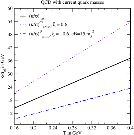
Figure 8: Variation of the ratio of thermal conductivity to electrical conductivity with temperature in the presence of momentum anisotropies both due to asymptotic expansion and strong magnetic field ($15$ $m_{\pi}^{2}$), where the current quark masses have been used.

In the isotropic medium, the ratio is found to increase linearly with temperature. When the isotropic medium is subjected to an expansion-driven anisotropy, $\kappa/\sigma_{\rm el}$ shows almost the same increasing behavior with temperature like in isotropic case, but its magnitude and slope (i.e. the Lorenz number) get enhanced. If the origin of anisotropy is strong magnetic field, then both the magnitude and the slope become smaller than the former descriptions. Thus in two different types of anisotropies we have observed nearly opposite behavior of $\kappa/\sigma_{\rm el}$, which can also be understood from the opposite behavior in electrical and thermal conductivities for the two aforesaid anisotropic mediums. This observation thus implies different Lorenz numbers ($\kappa/(\sigma_{\rm el}T)$) at the same temperature, depending on the anisotropies.

4.2 Knudsen number

The Knudsen number ($\Omega$) is required to be small for small deviation from equilibrium in the hydrodynamic regime, which is defined as

$$\Omega=\frac{\lambda}{L}~{},$$ (64)

where $\lambda$ denotes the mean free path and $L$ is the characteristic length scale of the system. One can calculate the mean free path by using the thermal conductivity ($\kappa$) of the medium,

$$\lambda=\frac{3\kappa}{vC_{V}}~{},$$ (65)

where $v$ is the relative speed and $C_{V}$ is the specific heat. Therefore the Knudsen number can be recast in terms of the thermal conductivity as

$$\Omega=\frac{3\kappa}{LvC_{V}}~{}.$$ (66)

In the calculation we have taken $v\simeq 1$, $L=3$ fm, and $C_{V}$ is evaluated from the energy-momentum tensor, i.e. $C_{V}=\partial(u_{\mu}T^{\mu\nu}u_{\nu})/\partial T$.

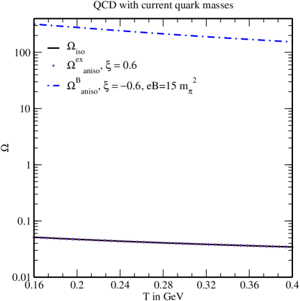
Figure 9: Variation of the Knudsen number with temperature in the presence of momentum anisotropies both due to asymptotic expansion and strong magnetic field ($15$ $m_{\pi}^{2}$), where the current quark masses have been used.

In an isotropic medium, the Knudsen number decreases with the increase of temperature, which explains that the mean free path becomes much smaller than the characteristic length scale of the system. As a result, the medium approaches equilibrium faster. When the medium exhibits a weak-momentum anisotropy due to the asymptotic expansion initially, the Knudsen number does not deviate considerably from its value in the isotropic medium (seen in figure 9). However if the origin of anisotropy is the strong magnetic field ($eB=15$ $m_{\pi}^{2}$), a significant deviation from the isotropic one can be seen, where the Knudsen number has a larger magnitude (denoted as dashed-dotted line in figure 9), which defies physical interpretation and urges us to use the quasiparticle model (seen in figure 15).

5 Quasiparticle description of hot QCD matter

Till now, we, in fact, have not incorporated any interactions among quarks and gluons in a thermal QCD medium either in the presence or absence of strong magnetic field. As a matter of fact, the magnitude and the variation of the electrical conductivity, thermal conductivity and Knudsen number become unrealistic. Hence we must resort to the quasiparticle description of particles, known as QPM, where different flavors acquire the medium generated masses, in addition to their current masses. The thermal mass is generated due to the interaction of quark with other particles of the medium, thus the quasiparticle model properly describes the collective properties of the medium. Earlier, this model was explained in different approaches such as the Nambu-Jona-Lasinio and PNJL based quasiparticle models [66, 67, 68], quasiparticle model based on Gribov-Zwanziger quantization [69, 70] etc. However, for our calculation, the effective mass (squared) of $i$-th flavor in a pure thermal medium is taken from [71],

$$m_{i}^{2}=m_{i0}^{2}+\sqrt{2}m_{i0}m_{iT}+m_{iT}^{2}~{},$$ (67)

where $m_{i0}$ and $m_{iT}$ are the current quark mass and the thermally generated mass of $i$-th flavor, respectively. The thermal mass is calculated in one loop in refs. [72, 73] as

$$m_{iT}^{2}=\frac{g^{\prime 2}T^{2}}{6}~{},$$ (68)

where $g^{\prime}$ is the running coupling that runs with the temperature of the medium. However, for a thermal medium in the presence of a strong magnetic field, the effective mass in thermal medium in eq. (67) can be generalized into

$$m_{i}^{2}=m_{i0}^{2}+\sqrt{2}m_{i0}m_{iT,B}+m_{iT,B}^{2}~{}.$$ (69)

Like the evaluation of $m_{iT}$, $m_{iT,B}$ could be similarly derived from the self-consistent Schwinger-Dyson equation by the quark self-energy for a thermal QCD medium in a strong magnetic field, which needs to be evaluated now.

As we know that the quark self-energy is given by

$$\Sigma(p)=-\frac{4}{3}g^{2}i\int{\frac{d^{4}k}{(2\pi)^{4}}}\left[\gamma_{\mu}{S(k)}\gamma^{\mu}{D(p-k)}\right],$$ (70)

where $4/3$ is the Casimir factor and $g$ is the running coupling that runs mainly with the magnetic field [74, 75] because the magnetic field is the largest energy scale for quarks in the strong magnetic field regime. The quark propagator, $S(K)$ in vacuum is modified in the presence of magnetic field and is given [76, 77] by the Schwinger proper-time method in the momentum space,

$$S(k)=ie^{-\frac{k^{2}_{\perp}}{|q_{i}B|}}\frac{\left(\gamma^{0}k_{0}-\gamma^{3}k_{z}+m_{i}\right)}{k^{2}_{\parallel}-m^{2}_{i}}\left(1-\gamma^{0}\gamma^{3}\gamma^{5}\right),$$ (71)

where the four vectors are defined below with the metric tensors: $g^{\mu\nu}_{\perp}={\rm{diag}}(0,-1,-1,0)$ and $g^{\mu\nu}_{\parallel}={\rm{diag}}(1,0,0,-1)$,

$$k_{\perp\mu}\equiv(0,k_{x},k_{y},0),~{}~{}k_{\parallel\mu}\equiv(k_{0},0,0,k_{z})~{}.$$

The gluon propagator in vacuum retains the same form even in the presence of magnetic field, i.e.

$$D^{\mu\nu}(p-k)=\frac{ig^{\mu\nu}}{(p-k)^{2}}~{}.$$ (72)

Next we obtain the form of quark and gluon propagators at finite temperature in the imaginary-time formalism and subsequently replace the energy integral ($\int\frac{dp_{0}}{2\pi}$) by sums over Matsubara frequencies, to get the form of self-energy (70) at finite temperature. However, in a strong magnetic field along $z$-direction, the transverse component of the momentum becomes vanishingly small ($k_{\perp}\approx 0$), so the exponential factor in eq. (71) becomes unity and the integration over the transverse component of the momentum becomes $|q_{i}B|$. Therefore the self-energy (70) at finite temperature in the SMF limit gets simplified into

$$\Sigma(p_{\parallel}) = \frac{2g^{2}}{3\pi^{2}}|q_{i}B|T\sum_{n}\int dk_{z}\frac{\left[\left(1+\gamma^{0}\gamma^{3}\gamma^{5}\right)\left(\gamma^{0}k_{0}-\gamma^{3}k_{z}\right)-2m_{i}\right]}{\left[k_{0}^{2}-\omega^{2}_{k}\right]\left[(p_{0}-k_{0})^{2}-\omega_{pk}^{2}\right]}$$ (73)

$$= \frac{2g^{2}|q_{i}B|}{3\pi^{2}}\int dk_{z}\left[(\gamma^{0}+\gamma^{3}\gamma^{5})L^{1}-(\gamma^{3}+\gamma^{0}\gamma^{5})k_{z}L^{2}\right],$$

where $\omega^{2}_{k}=k_{z}^{2}+m_{i}^{2}$, $\omega_{pk}^{2}=(p_{z}-k_{z})^{2}$ and $L^{1}$ and $L^{2}$ are the two frequency sums, which are given by

$$L^{1}=T\sum_{n}k_{0}~{}\frac{1}{\left[k_{0}^{2}-\omega_{k}^{2}\right]}\frac{1}{\left[(p_{0}-k_{0})^{2}-\omega_{pk}^{2}\right]}~{},$$ (74)

$$L^{2}=T\sum_{n}\frac{1}{\left[k_{0}^{2}-\omega_{k}^{2}\right]}\frac{1}{\left[(p_{0}-k_{0})^{2}-\omega_{pk}^{2}\right]}~{}.$$ (75)

After calculating the above frequency sums [16, 78], the self-energy (73) can be simplified further into

$$\Sigma(p_{\parallel})=\frac{g^{2}|q_{i}B|}{3\pi^{2}}\int\frac{dk_{z}}{\omega_{k}}\left[\frac{1}{e^{\beta\omega_{k}}-1}+\frac{1}{e^{\beta\omega_{k}}+1}\right]\left[\frac{\gamma^{0}p_{0}+\gamma^{3}p_{z}}{p_{\parallel}^{2}}+\frac{\gamma^{0}\gamma^{5}p_{z}+\gamma^{3}\gamma^{5}p_{0}}{p_{\parallel}^{2}}\right],$$ (76)

which yields the following form, after the integration over $k_{z}$,

$$\Sigma(p_{\parallel})=\frac{g^{2}|q_{i}B|}{3\pi^{2}}\left[\frac{\pi T}{2m_{i}}-\ln(2)\right]\left[\frac{\gamma^{0}p_{0}}{p_{\parallel}^{2}}+\frac{\gamma^{3}p_{z}}{p_{\parallel}^{2}}+\frac{\gamma^{0}\gamma^{5}p_{z}}{p_{\parallel}^{2}}+\frac{\gamma^{3}\gamma^{5}p_{0}}{p_{\parallel}^{2}}\right].$$ (77)

Let us explore the covariant structure of the quark self-energy at finite temperature in an additional presence of magnetic field, which can in general be written [79, 80] as

$$\Sigma(p_{\parallel})=A\gamma^{\mu}u_{\mu}+B\gamma^{\mu}b_{\mu}+C\gamma^{5}\gamma^{\mu}u_{\mu}+D\gamma^{5}\gamma^{\mu}b_{\mu}~{},$$ (78)

where $A$, $B$, $C$ and $D$ are the form factors, and $u^{\mu}$ (1,0,0,0) and $b^{\mu}$ (0,0,0,-1) specify the preferred directions of the heat bath and the magnetic field, respectively. These vectors are responsible for breaking the Lorentz and rotational symmetries, respectively. We have obtained the form factors in LLL approximation as

$$A=\frac{1}{4}{\rm Tr}\left[\Sigma\gamma^{\mu}u_{\mu}\right]=\frac{g^{2}|q_{i}B|}{3\pi^{2}}\left[\frac{\pi T}{2m_{i}}-\ln(2)\right]\frac{p_{0}}{p_{\parallel}^{2}}~{},$$ (79)

$$B=-\frac{1}{4}{\rm Tr}\left[\Sigma\gamma^{\mu}b_{\mu}\right]=\frac{g^{2}|q_{i}B|}{3\pi^{2}}\left[\frac{\pi T}{2m_{i}}-\ln(2)\right]\frac{p_{z}}{p_{\parallel}^{2}}~{},$$ (80)

$$C=\frac{1}{4}{\rm Tr}\left[\gamma^{5}\Sigma\gamma^{\mu}u_{\mu}\right]=-\frac{g^{2}|q_{i}B|}{3\pi^{2}}\left[\frac{\pi T}{2m_{i}}-\ln(2)\right]\frac{p_{z}}{p_{\parallel}^{2}}~{},$$ (81)

$$D=-\frac{1}{4}{\rm Tr}\left[\gamma^{5}\Sigma\gamma^{\mu}b_{\mu}\right]=-\frac{g^{2}|q_{i}B|}{3\pi^{2}}\left[\frac{\pi T}{2m_{i}}-\ln(2)\right]\frac{p_{0}}{p_{\parallel}^{2}}~{},$$ (82)

which indicates that $C=-B$ and $D=-A$.

The quark self-energy (78) can also be written in terms of the right-handed ($P_{R}=(1+\gamma^{5})/2$) and left-handed ($P_{L}=(1-\gamma^{5})/2$) chiral projection operators,

$$\Sigma(p_{\parallel})=P_{R}\left[(A+C)\gamma^{\mu}u_{\mu}+(B+D)\gamma^{\mu}b_{\mu}\right]P_{L}+P_{L}\left[(A-C)\gamma^{\mu}u_{\mu}+(B-D)\gamma^{\mu}b_{\mu}\right]P_{R}~{},$$ (83)

which becomes simplified as

$$\Sigma(p_{\parallel})=P_{R}\left[(A-B)\gamma^{\mu}u_{\mu}+(B-A)\gamma^{\mu}b_{\mu}\right]P_{L}+P_{L}\left[(A+B)\gamma^{\mu}u_{\mu}+(B+A)\gamma^{\mu}b_{\mu}\right]P_{R}~{},$$ (84)

after the substitutions $C=-B$ and $D=-A$.

Therefore the effective quark propagator is obtained from the self-consistent Schwinger-Dyson equation in the presence of a strong magnetic field,

$$S^{-1}(p_{\parallel})=\gamma^{\mu}p_{\parallel\mu}-\Sigma(p_{\parallel})~{},$$ (85)

which in turn takes the following form in terms of projection operators,

$$S^{-1}(p_{\parallel})=P_{R}\gamma^{\mu}X_{\mu}P_{L}+P_{L}\gamma^{\mu}Y_{\mu}P_{R}~{},$$ (86)

where

$$\gamma^{\mu}X_{\mu}=\gamma^{\mu}p_{\parallel\mu}-(A-B)\gamma^{\mu}u_{\mu}-(B-A)\gamma^{\mu}b_{\mu}~{},$$ (87)

$$\gamma^{\mu}Y_{\mu}=\gamma^{\mu}p_{\parallel\mu}-(A+B)\gamma^{\mu}u_{\mu}-(B+A)\gamma^{\mu}b_{\mu}~{}.$$ (88)

Now the effective propagator is written as

$$S(p_{\parallel})=\frac{1}{2}\left[P_{R}\frac{\gamma^{\mu}Y_{\mu}}{Y^{2}/2}P_{L}+P_{L}\frac{\gamma^{\mu}X_{\mu}}{X^{2}/2}P_{R}\right],$$ (89)

where

$$\frac{X^{2}}{2}=X_{1}^{2}=\frac{1}{2}\left[p_{0}-(A-B)\right]^{2}-\frac{1}{2}\left[p_{z}+(B-A)\right]^{2}~{},$$ (90)

$$\frac{Y^{2}}{2}=Y_{1}^{2}=\frac{1}{2}\left[p_{0}-(A+B)\right]^{2}-\frac{1}{2}\left[p_{z}+(B+A)\right]^{2}~{}.$$ (91)

Thus the thermal mass (squared) at finite temperature and strong magnetic field is finally obtained by taking the $p_{0}=0,p_{z}\rightarrow 0$ limit of either $X_{1}^{2}$ or $Y_{1}^{2}$ (because both of them are equal),

$$m_{iT,B}^{2}=X_{1}^{2}\Big{|}_{p_{0}=0,p_{z}\rightarrow 0}=Y_{1}^{2}\Big{|}_{p_{0}=0,p_{z}\rightarrow 0}=\frac{g^{2}|q_{i}B|}{3\pi^{2}}\left[\frac{\pi T}{2m_{i}}-\ln(2)\right],$$ (92)

which depends on both temperature and magnetic field.

In the quasiparticle description of particles, the distribution functions now contain the effective masses of the particles. Therefore, the distribution functions in the isotropic medium as well as in the expansion-driven anisotropic medium use the $T$-dependent effective mass (67), whereas the distribution function in the strong magnetic field-driven anisotropic medium uses the $T$ and $B$-dependent effective mass (69). So, from figures 10 and 11, we noticed that the behaviors of ratios ($f^{\rm ex}_{\rm aniso}/f_{\rm iso}$ and $f^{\rm B}_{\rm aniso}/f_{\rm iso}$) get flipped in comparison to their respective behavior in ideal case (as in figures 4 and 5). As the transport coefficients such as the electrical conductivity and the thermal conductivity are expressed in terms of the distribution function at finite temperature and/or magnetic field, so the knowledge about the behavior of distribution function in the QPM description is useful in understanding the transport properties of the hot QCD medium.

In the coming subsections we are going to discuss the results on the electrical conductivity, thermal conductivity and their applications using the quasiparticle model with three flavors ($u$, $d$ and $s$).

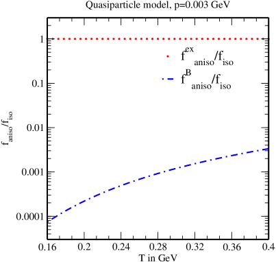
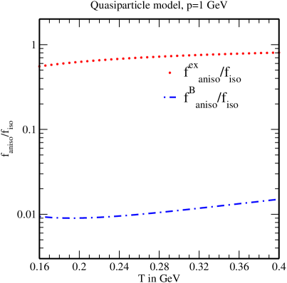
a	b

Figure 10: Variation of the ratio $f_{\rm aniso}/f_{\rm iso}$ with temperature in the presence of momentum anisotropies both due to asymptotic expansion and strong magnetic field ($15$ $m_{\pi}^{2}$) at (a) low momentum and (b) high momentum, where the effective quark mass has been used.

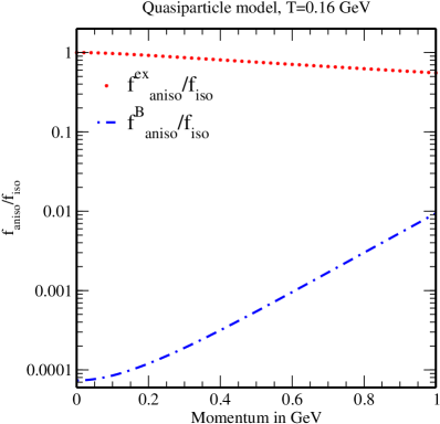
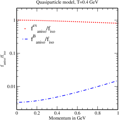
a	b

Figure 11: Variation of the ratio $f_{\rm aniso}/f_{\rm iso}$ with momentum in the presence of momentum anisotropies both due to asymptotic expansion and strong magnetic field ($15$ $m_{\pi}^{2}$) at (a) low temperature and (b) high temperature, where the effective quark mass has been used.

5.1 Electrical conductivity

With the quasiparticle description as input, we have now recomputed the electrical conductivity by substituting the temperature-dependent effective mass (67) into its expressions for the isotropic (9) and expansion-driven anisotropic (15) mediums, and the temperature and magnetic field-dependent effective mass (69) into its expression for the magnetic field-driven anisotropic medium (30). We have replotted $\sigma_{\rm el}$ as a function of temperature in figure 12 and found that there is an overall decrease in $\sigma_{\rm el}$. Interestingly, for a magnetic field-driven weak-momentum anisotropy (denoted by dashed-dotted line), the magnitude of $\sigma_{\rm el}$ now becomes smaller, which is at par with its counterparts in isotropic and expansion-driven anisotropic mediums. However, $\sigma_{\rm el}$ for the magnetic field-driven anisotropic medium, now decreases with the temperature, which is opposite to its variation in the expansion-driven anisotropy. The above differences in the $\sigma_{\rm el}$’s can be understood qualitatively from the distributions seen in figures 10 and 11, the relaxation time in the absence and presence of magnetic field, and the phase-space factor (which gets affected by the strong magnetic field only). We are now convinced that the quasiparticle description of particles tames the unusually large value of $\sigma_{\rm el}$ in the strong magnetic field.

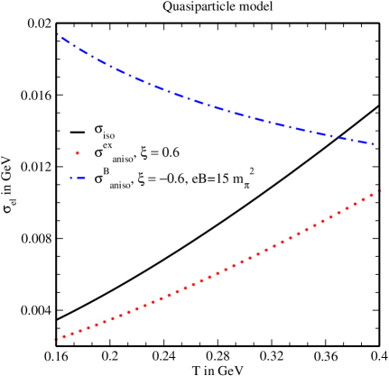
Figure 12: Variation of electrical conductivity with temperature in the presence of momentum anisotropies both due to asymptotic expansion and strong magnetic field ($15$ $m_{\pi}^{2}$), where the effective quark masses have been used.

5.2 Thermal conductivity

We have also calculated the thermal conductivity with the quasiparticle description by substituting the temperature-dependent effective mass (67) into its expressions for the isotropic (44) and expansion-driven anisotropic (50) mediums, and the temperature and magnetic field-dependent effective mass (69) into its expression for the magnetic field-driven anisotropic medium (62). Figure 13 plots the variation of $\kappa$ with temperature for the isotropic medium, expansion- and strong magnetic field-driven anisotropic mediums with the quasiparticle description. The effects of quasiparticle description on the thermal conductivity can again be understood through the distribution functions with quasiparticle masses in figures 10 and 11, and the relaxation time in the absence and presence of magnetic field. For the isotropic as well as expansion-driven anisotropic mediums, $\kappa$ is found to increase with temperature as in ideal case. The only noticeable finding is that, although the magnitude of $\kappa$ for the strong magnetic field-driven anisotropic medium is still larger than in isotropic medium but it has now become smaller and comparable with the value in isotropic medium at higher temperature within the SMF limit ($eB\gg T^{2}$).

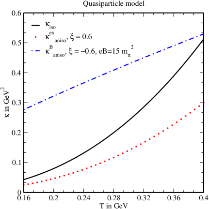
Figure 13: Variation of thermal conductivity with temperature in the presence of momentum anisotropies both due to asymptotic expansion and strong magnetic field ($15$ $m_{\pi}^{2}$), where the effective quark masses have been used.

5.3 Wiedemann-Franz law

Wiedemann-Franz law makes us understand the relation between the charge transport and the heat transport in a system. Here we have revisited the law in quasiparticle description of particles, unlike the ideal description of particles earlier in previous subsection 4.1. In figure 14 we found that the ratio, $\kappa/\sigma_{\rm el}$ in magnetic field-driven anisotropy increases linearly with the temperature, with a magnitude larger than that in isotropic medium and smaller than that in expansion-driven anisotropic medium. So, it can be used to distinguish the anisotropies of different origins. Thus, the Lorenz number, defined as the slope of the ratio ($\kappa/\sigma_{\rm el}$) versus $T$ graph, is smaller in the strong magnetic field-driven anisotropic medium as compared to its value in the expansion-driven anisotropic medium.

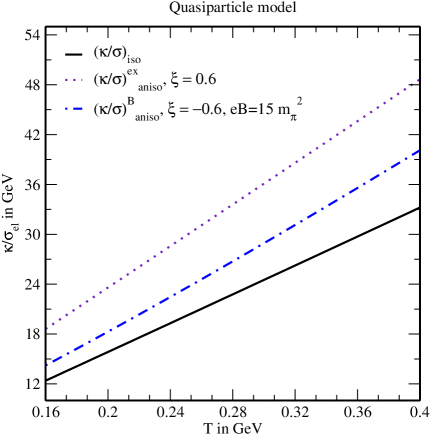
Figure 14: Variation of the ratio of thermal conductivity to electrical conductivity with temperature in the presence of momentum anisotropies both due to asymptotic expansion and strong magnetic field ($15$ $m_{\pi}^{2}$), where the effective quark masses have been used.

5.4 Knudsen number

We have seen earlier that for a strong magnetic field-driven anisotropic medium, the Knudsen number ($\Omega$) in the ideal case (seen in figure 9) was very large. As a result, the thermal medium in the presence of strong magnetic field deviates much away from its equilibrium which is, however, not desirable. This is exactly circumvented here in the quasiparticle description in figure 15, where we have found that $\Omega$ has now been decreased drastically in the presence of strong magnetic field at par with the estimates for $B=0$ cases. However, there is an overall decrease of Knudsen number for all cases. Thus in the quasiparticle description, the probability of finding the system to be in local equilibrium is higher, due to the smaller value of Knudsen number.

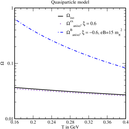
Figure 15: Variation of the Knudsen number with temperature in the presence of momentum anisotropies both due to asymptotic expansion and strong magnetic field ($15$ $m_{\pi}^{2}$), where the effective quark masses have been used.

6 Conclusions and future outlook

In this work, we have studied the effect of strong magnetic field-driven anisotropy on the transport coefficients such as electrical conductivity and thermal conductivity of the hot QCD matter and compared them with their behavior in the expansion-driven anisotropy. In order to find these conductivities we have solved the relativistic Boltzmann transport equation in relaxation-time approximation, where the interactions are incorporated through the distribution function within the quasiparticle approach at finite temperature and strong magnetic field. We have also compared the conductivities with their corresponding values in the ideal scenario.

First we have revisited the formulation of electrical and thermal conductivities for the isotropic thermal medium and then calculated these for the expansion-induced anisotropic thermal medium. Using the value of electrical conductivity we have then observed the variation of magnetic field with time and this explains that the lifetime of the strong magnetic field becomes larger for an electrically conducting medium as compared to the vacuum, hence the strong magnetic field is expected to affect the charge transport and the heat transport in the QCD medium and this motivated us to derive the aforesaid conductivities for a thermal medium in the presence of strong magnetic field-induced anisotropy. We have observed that both the electrical and thermal conductivities have larger values in the presence of strong magnetic field-driven anisotropy as compared to their respective values in the isotropic medium, however if the anisotropy is induced due to asymptotic expansion, then the values of the conductivities are seen to get lowered than their values in the isotropic medium. So, in the two different types of anisotropic mediums, we noticed nearly opposite behavior of conductivities. The noticeably large values of conductivities in a strong magnetic field in case of ideal description are avoided using the quasiparticle description. Next, we have studied the Wiedemann-Franz law to see the relative behavior of electrical conductivity and thermal conductivity, where their ratio ($\kappa/\sigma_{\rm el}$) is found to increase linearly with temperature, but with a magnitude larger than in isotropic medium and smaller than in expansion-driven anisotropic medium, thus it can be used as a promising tool to probe the anisotropies of different sources. Then, we have calculated the Knudsen number to observe whether the system is still in equilibrium in the presence of weak-momentum anisotropy which may be caused by either sources. We have found that, in the quasiparticle description, the Knudsen number becomes less than one, thus the medium may remain in local equilibrium even in the presence of weak-momentum anisotropy.

In summary, the anisotropy affects the electrical and thermal conductivities, which in turn affects the Lorenz number, Knudsen number significantly. Thus it becomes imperative to suggest on the possible signatures of the abovementioned observations in heavy-ion phenomenology as our future plan. Chiral magnetic effect could be one such observable effect, because this effect is associated with the generation of current along the direction of magnetic field, which in turn depends on the magnitude of the electrical conductivity [14]. On the other hand the thermal conductivity could be used as a handle to decipher the assumption of local equilibrium in terms of mean free path via the inclusive production of dilepton and photon. It has been observed previously that the dilepton and photon yields get enhanced in the presence of weak-momentum anisotropy due to initial asymptotic expansion [32, 33]. Therefore, a similar study in the dilepton and photon productions due to the magnetic field-driven anisotropy needs to be done and the comparison with the former anisotropy could be an indicator of the findings in thermal conductivity.

7 Acknowledgment

One of us (B. K. Patra) is thankful to Council of Scientific and Industrial Research (No.: 03(1407)/17/EMR-II), Government of India for the financial support of this work.

References

- [1] E. L. Feinberg, Nuovo Cim. A 34, 391 (1976).
- [2] E. V. Shuryak, Phys. Lett. B 78, 150 (1978).
- [3] J. I. Kapusta, P. Lichard and D. Seibert, Phys. Rev. D 44, 2774 (1991).
- [4] J. P. Blaizot and J. Y. Ollitrault, Phys. Rev. Lett. 77, 1703 (1996).
- [5] Helmut Satz, Nucl. Phys. A 783, 249 (2007).
- [6] R. Rapp, D. Blaschke and P. Crochet, Prog. Part. Nucl. Phys. 65, 209 (2010).
- [7] R. S. Bhalerao and J. Y. Ollitrault, Phys. Lett. B 641, 260 (2006).
- [8] S. A. Voloshin, A. M. Poskanzer, A. Tang, G. Wang, Phys. Lett. B 659, 537 (2008).
- [9] X. N. Wang and M. Gyulassy, Phys. Rev. Lett. 68, 1480 (1992).
- [10] K. Adcox et al., Phys. Rev. Lett. 88, 022301 (2002).
- [11] S. Chatrchyan et al., Phys. Rev. C 84, 024906 (2011).
- [12] V. Skokov, A. Illarionov, and V. Toneev, Int. J. Mod. Phys. A 24, 5925 (2009).
- [13] P. F. Kolb and U. W. Heinz, In Hwa, R.C. (ed.) et al., Quark gluon plasma, 634 (2003).
- [14] K. Fukushima, D. E. Kharzeev and H. J. Warringa, Phys. Rev. D 78, 074033 (2008).
- [15] Y. Hirono, M. Hongo and T. Hirano, Phys. Rev. C 90, 021903 (2014).
- [16] J. I. Kapusta and C. Gale, “Finite Temperature Field Theory Principles and Applications”, Cambridge University Press, 2006.
- [17] P. V. Buividovich, M. N. Chernodub, D. E. Kharzeev, T. Kalaydzhyan, E. V. Luschevskaya and M. I. Polikarpov, Phys. Rev. Lett. 105, 132001 (2010).
- [18] Seung-il Nam, Phys. Rev. D 86, 033014 (2012).
- [19] D. E. Kharzeev, Prog. Part. Nucl. Phys. 75, 133 (2014).
- [20] D. Satow, Phys. Rev. D 90, 034018 (2014).
- [21] S. Pu, S. Y. Wu and D. L. Yang, Phys. Rev. D 91, 025011 (2015).
- [22] K. Hattori and D. Satow, Phys. Rev. D 94, 114032 (2016).
- [23] M. Kurian and V. Chandra, Phys. Rev. D 96, 114026 (2017).
- [24] K. Aamodt et al., Phys. Lett. B 696, 30 (2011).
- [25] P. Foka and M. A. Janik, Rev. Phys. 1, 172 (2016).
- [26] K. Tuchin, Phys. Rev. D 91, 033004 (2015).
- [27] G. Basar, D. E. Kharzeev and V. Skokov, Phys. Rev. Lett. 109, 202303 (2012).
- [28] K. Fukushima and K. Mameda, Phys. Rev. D 86, 071501(R) (2012).
- [29] D. Kabat, K. Lee and E. Weinberg, Phys. Rev. D 66, 014004 (2002).
- [30] A. Dumitru, Y. Guo, Á. Mócsy and M. Strickland, Phys. Rev. D 79, 054019 (2009).
- [31] A. Dumitru, Y. Guo and M. Strickland, Phys. Lett. B 662, 37 (2008).
- [32] M. Martinez and M. Strickland, Phys. Rev. C 78, 034917 (2008).
- [33] R. Ryblewski and M. Strickland, Phys. Rev. D 92, 025026 (2015).
- [34] A. Mukherjee, M. Mandal and P. Roy, Eur. Phys. J. A 53, 81 (2017).
- [35] L. Bhattacharya, R. Ryblewski and M. Strickland, Phys. Rev. D 93, 065005 (2016).
- [36] L. Thakur, N. Haque, U. Kakade and B. K. Patra, Phys. Rev. D 88, 054022 (2013).
- [37] P. K. Srivastava, L. Thakur and B. K. Patra, Phys. Rev. C 91, 044903 (2015).
- [38] L. Thakur, P. K. Srivastava, G. P. Kadam, M. George and H. Mishra, Phys. Rev. D 95, 096009 (2017).
- [39] R. S. Bhalerao, M. Luzum and J.-Y. Ollitrault, Phys. Rev. C 84, 054901 (2011).
- [40] U. Heinz, Z. Qiu and C. Shen, Phys. Rev. C 87, 034913 (2013).
- [41] R. Mahajan, M. Barkeshli and S. A. Hartnoll, Phys. Rev. B 88, 125107 (2013).
- [42] C. Proust, K. Behnia, R. Bel, D. Maude and S. I. Vedeneev, Phys. Rev. B 72, 214511 (2005).
- [43] J. Crossno et al., Science 351, 1058 (2016).
- [44] A. Harutyunyan, D. H. Rischke and A. Sedrakian, Phys. Rev. D 95, 114021 (2017).
- [45] S. Mitra and V. Chandra, Phys. Rev. D 96, 094003 (2017).
- [46] A. Muronga, Phys. Rev. C 76, 014910 (2007).
- [47] A. Puglisi, S. Plumari and V. Greco, Phys. Rev. D 90, 114009 (2014).
- [48] S. Yasui and S. Ozaki, Phys. Rev. D 96, 114027 (2017).
- [49] S. Mitra and V. Chandra, Phys. Rev. D 94, 034025 (2016).
- [50] M. Greif, I. Bouras, C. Greiner and Z. Xu, Phys. Rev. D 90, 094014 (2014).
- [51] B. Feng, Phys. Rev. D 96, 036009 (2017).
- [52] S. Gupta, Phys. Lett. B 597, 57 (2004).
- [53] G. Aarts, C. Allton, A. Amato, P. Giudice, S. Hands and J.-I. Skullerud, JHEP 1502, 186 (2015).
- [54] H.-T. Ding, O. Kaczmarek and F. Meyer, Phys. Rev. D 94, 034504 (2016).
- [55] C. Crecignani and G. M. Kremer, “The Relativistic Boltzmann Equation: Theory and Applications” (Boston, Birkhiiuser, 2002).
- [56] A. Hosoya and K. Kajantie, Nucl. Phys. B 250, 666 (1985).
- [57] P. Romatschke and M. Strickland, Phys. Rev. D 68, 036004 (2003).
- [58] K. Tuchin, Adv. High Energy Phys. 2013, 490495 (2013).
- [59] V. P. Gusynin and A. V. Smilga, Phys. Lett. B 450, 267 (1999).
- [60] S. Rath and B. K. Patra, JHEP 1712, 098 (2017).
- [61] S. Rath and B. K. Patra, arXiv:1806.03008 [hep-th].
- [62] V. P. Gusynin, V. A. Miransky and I. A. Shovkovy, Nucl. Phys. B 462, 249 (1996).
- [63] F. Bruckmann, G. Endrődi, M. Giordano, S. D. Katz, T. G. Kovács, F. Pittler and J. Wellnhofer, Phys. Rev. D 96, 074506 (2017).
- [64] Koichi Hattori, Shiyong Li, Daisuke Satow and Ho-Ung Yee, Phys. Rev. D 95, 076008 (2017).
- [65] M. Greif, F. Reining, I. Bouras, G. S. Denicol, Z. Xu and C. Greiner, Phys. Rev. E 87, 033019 (2013).
- [66] K. Fukushima, Phys. Lett. B 591, 277 (2004).
- [67] S. K. Ghosh, T. K. Mukherjee, M. G. Mustafa and R. Ray, Phys. Rev. D 73, 114007 (2006).
- [68] H. Abuki and K. Fukushima, Phys. Lett. B 676, 57 (2009).
- [69] N. Su and K. Tywoniuk, Phys. Rev. Lett. 114, 161601 (2015).
- [70] W. Florkowski, R. Ryblewski, N. Su and K. Tywoniuk, Phys. Rev. C 94, 044904 (2016).
- [71] V. M. Bannur, JHEP 0709, 046 (2007).
- [72] E. Braaten and R. D. Pisarski, Phys. Rev. D 45, R1827 (1992).
- [73] A. Peshier, B. Kämpfer and G. Soff, Phys. Rev. D 66, 094003 (2002).
- [74] E. J. Ferrer, V. de la Incera and X. J. Wen, Phys. Rev. D 91, 054006 (2015).
- [75] M. A. Andreichikov, V. D. Orlovsky and Yu. A. Simonov, Phys. Rev. Lett. 110, 162002 (2013).
- [76] J. Schwinger, Phys. Rev. 82, 664 (1951).
- [77] Wu-yang Tsai, Phys. Rev. D 10, 2699 (1974).
- [78] M. L. Bellac, “Thermal Field Theory”, Cambridge University Press, 1996.
- [79] A. Ayala, J. J. Cobos-Martínez, M. Loewe, M. E. Tejeda-Yeomans and R. Zamora, Phys. Rev. D 91, 016007 (2015).
- [80] B. Karmakar, R. Ghosh, A. Bandyopadhyay, N. Haque and M. G. Mustafa, arXiv:1902.02607 [hep-ph].