Iterative approach to arbitrary nonlinear optical response functions of graphene

Abstract

Two-dimensional materials constitute an exciting platform for nonlinear optics with large nonlinearities that are tunable by gating. Hence, gate-tunable harmonic generation and intensity-dependent refraction have been observed in e.g. graphene and transition-metal dichalcogenides, whose electronic structures are accurately modelled by the (massive) Dirac equation. We exploit on the simplicity of this model and demonstrate here that arbitrary nonlinear response functions follow from a simple iterative approach. The power of this approach is illustrated by analytical expressions for harmonic generation and intensity-dependent refraction, both computed up to ninth order in the pump field. Moreover, the results allow for arbitrary band gaps and gating potentials. As illustrative applications, we consider (i) gate-dependence of third- and fifth-harmonic generation in gapped and gapless graphene, (ii) intensity-dependent refractive index of graphene up to ninth order, and (iii) intensity-dependence of high-harmonic generation.

Nonlinear optical (NLO) response encompasses a large class of light matter interactions Boyd (2008); Shen (2002); Franken and Ward (1963); Bloembergen (1982); Axt and Mukamel (1998); Kuzyk et al. (2013), including processes such as harmonic generation and self-focusing of light, that have proven useful in a number of applications in nonlinear spectroscopy and in optoelectronic devices. Recent progress in the fabrication of 2D materials has produced a new fertile class of materials with large nonlinear susceptibilities Autere et al. (2018). Recent reports include measurements of high harmonic generation (HHG) Yoshikawa et al. (2017); Hafez et al. (2018) and intensity dependent refractive index Lim et al. (2011); Mohsin et al. (2015) in graphene and in transition metal dichalcogenides (TMDs) Liu et al. (2016). In addition, it has been shown that the NLO response can be tuned by electrostatic doping Soavi et al. (2018); Jiang et al. (2018); Zhang et al. (2018) and significant progress has been made in measuring even-order NLO response in TMDs Wang et al. (2015); Säynätjoki et al. (2017). Furthermore, the nonlinearities in 2D materials can be significantly enhanced by several mechanisms such as plasmons Cox et al. (2017); Kundys et al. (2018); Wang et al. (2018), polaritonic effects Wild et al. (2018), and metasurfaces Rosolen et al. (2018).

Compared with the linear response, calculations of NLO processes in crystals are significantly more complex. Whereas the linear response results from purely inter- or intraband processes, the NLO response contains not only these processes, but also mixed ones involving both inter- and intraband motion of electrons Aversa and Sipe (1995); Pedersen (2015); Taghizadeh et al. (2017); Hipolito et al. (2018). To circumvent this complexity, the NLO response has been characterized using several theoretical methods, each with its own merits and shortcomings: (i) perturbative expansion of the reduced density matrix Cheng et al. (2014); Rostami and Polini (2016); Hipolito et al. (2018); (ii) time-dependent techniques Tamaya et al. (2016); Chizhova et al. (2017); Dimitrovski et al. (2017); Mikhailov (2017); (iii) Wannier representation Catoire et al. (2018). The perturbative method offers a feasible approach to specific processes at a fixed frequency and power of the external field. The standard approach expands all matrix elements in unperturbed eigenstates, leading to increasingly complicated sum-over-states expressions for high-order processes. Still, within the perturbative regime, highly accurate results are obtained and in simple few-band systems such as the Dirac Hamiltonian, closed form solutions can often be found. These allow for characterization with respect to external parameters, for instance doping and temperature Cheng et al. (2014); Rostami and Polini (2016); Hipolito et al. (2018). Yet, the growth in complexity associated with mixed inter- and intraband motion makes calculations extremely cumbersome beyond third order. The complicated nature of the general third-order response Hipolito et al. (2018) testifies to this complexity. Methods (ii) and (iii) can be applied to study the NLO response at field strengths beyond the perturbative regime, as these intrinsically include contributions from all powers of the external field. But, in contrast to perturbative approaches, these methods rely extensively on numerical techniques for the integration of the equation of motion and for the Fourier transforms required to analyze the response in frequency domain, thus making the characterization of the NLO response with respect to external parameters an elaborate numerical process Tamaya et al. (2016); Chizhova et al. (2017); Dimitrovski et al. (2017); Mikhailov (2017).

In the present letter, we study the (massive and massless) Dirac Hamiltonian as a model of graphene and TMDs. For this important class of materials, we bridge a key shortcoming found in perturbative techniques by evaluating the current density response via an iterative solution. This approach allows for the evaluation of arbitrarily high order response functions. As an illustration, we compute all response functions up to ninth order for (gapped) graphene . The massive Dirac Hamiltonian Semenoff (1984) with a external vector potential $\mathbf{A}=\mathbf{A}_{0}\sin(\omega t)$ reads, using the minimal coupling (velocity gauge), Peres (2010)

$$H=v_{F}(\hbar\bm{\kappa}+e\mathbf{A})\cdot\bm{\sigma}+\hbar\Delta\sigma_{z},$$ (1)

where $v_{F}\sim 10^{6}\ \mathrm{m/s}$ is the Fermi velocity, $\bm{\kappa}$ is the wavevector, $\bm{\sigma}$ are the Pauli matrices, $\Delta\geq 0$ is the mass term, and $e>0$. This model leads to a gapped band structure with energy gap $E_{g}=2\hbar\Delta$, and doping is including via a non-vanishing Fermi level $\hbar\mu$. Hence, for pristine graphene, we take $\Delta=0$. The key features of the electronic structure are shown in Fig. 1(a). The Dirac Hamiltonian has proven extremely useful for systems with threefold rotation symmetry. It allows for accurate analytic characterization of several physical properties in graphene Castro Neto et al. (2009) and in the vast class of TMDs Xiao et al. (2012).

The time evolution of the wave function $\psi$ governed by $i\hbar\dot{\psi}=H\psi$ is found by expanding in the eigenstates $u_{1,2}$ of the unperturbed Hamiltonian, i.e. taking $\mathbf{A}=0$. We write the general wave function as

$$\psi=[a(t)u_{1}+b(t)u_{2}]\exp[i(\bm{\kappa}\cdot\mathbf{r}+\epsilon t)],$$ (2)

with energy dispersion $\epsilon=\sqrt{\Delta^{2}+k^{2}}$ (in frequency units), and $k=v_{F}|\bm{\kappa}|$. Furthermore, we focus on the response to a normally incident, linearly polarized monochromatic field, $\mathbf{A}=A\mathbf{e}_{x}$ and define $\mathcal{A}(t)=v_{F}eA_{0}\sin(\omega t)/\hbar=\mathcal{A}_{0}\sin(\omega t)$, which is related to the electric field $\mathcal{E}(t)=\mathcal{E}_{0}\cos(\omega t)$ by $\mathcal{E}_{0}=-\omega A_{0}$. The time evolution of the coefficients follows from $\dot{a}(t)=i\mathcal{A}(t)[a(t)F-b(t)G]$ and $i\dot{b}(t)=\mathcal{A}(t)G^{*}a(t)+[2\epsilon+\mathcal{A}(t)F]b(t)$, where $F=\sqrt{\epsilon^{2}-\Delta^{2}}\cos(\theta)/\epsilon$ and $G=[\Delta\cos(\theta)-i\epsilon\sin(\theta)]/\epsilon$ arise from matrix elements of the velocity operator. The coefficients then determine the reduced density matrix, whose matrix elements read $\rho_{11}=|a|^{2}$, $\rho_{22}=|b|^{2}$ and $\rho_{21}=a^{*}b$. In turn, their time evolution is governed by

$$i\dot{\mathcal{N}} =-2\mathcal{A}(t)(\mathcal{P}G-G^{*}\mathcal{P}^{*}),$$ (3a)

$$i\dot{\mathcal{P}} =-\mathcal{A}(t)G^{*}\mathcal{N}+2\big{[}\mathcal{A}(t)F+\epsilon]\mathcal{P},$$ (3b)

where $\mathcal{N}=\rho_{22}-\rho_{11}$ and $\mathcal{P}=\rho_{21}$ define the population difference and coherence, respectively. Finally, the current density is evaluated via the expectation value of the current density operator $j=-eg_{s}g_{v}(2\pi)^{-2}v_{F}\int\mathcal{J}d\bm{\kappa}$, where the dimensionless integrand for the current density response is defined by $\mathcal{J}=\sum_{mn}v_{nm}\rho_{mn}/v_{F}=F\mathcal{N}+\mathcal{P}G+G^{*}\mathcal{P}^{*}$ using the matrix elements $v_{nm}$ of the velocity operator $\hat{v}_{x}=v_{F}\hat{\sigma}_{x}$. Here, $g_{s}=2$ and $g_{v}=2$ are spin and valley degeneracies, respectively.

The iterative sequence is found by considering the first- and second-order time derivatives of $\mathcal{J}$ that read

$$\mathcal{A}(t)\dot{\mathcal{J}} =-\epsilon\dot{\mathcal{N}},$$ (4a)

$$\ddot{\mathcal{J}} =4\epsilon\big{[}\mathcal{A}(t)+\epsilon F\big{]}\mathcal{N}-4\epsilon\big{[}\mathcal{A}(t)F+\epsilon\big{]}\mathcal{J}.$$ (4b)

Using a time-harmonic expansion for the integrand $\mathcal{J}=\sum_{n}\mathcal{J}_{n}e^{-in\omega t}$ and for the population $\mathcal{N}=\sum_{n}\mathcal{N}_{n}e^{-in\omega t}$, the dynamical equations can be cast as

$$\mathcal{A}_{0}[(n-1)\mathcal{J}_{n-1}-(n+1)\mathcal{J}_{n+1}] =2in\epsilon\mathcal{N}_{n},$$ (5a)

$$(4\epsilon^{2}-n^{2}\omega^{2})\mathcal{J}_{n} =4\epsilon^{2}F\mathcal{N}_{n}-2i\epsilon\mathcal{A}_{0}F(\mathcal{J}_{n-1}-\mathcal{J}_{n+1})$$

$$+2i\epsilon\mathcal{A}_{0}(\mathcal{N}_{n-1}-\mathcal{N}_{n+1}),$$ (5b)

where $n\in\mathbb{Z}$ defines the Fourier order. The final iterative series for the integrand is identified by making use of an expansion with respect to powers of the external field $\mathcal{J}_{n}=\sum_{j\geq n}\mathcal{J}_{n}^{(j)}\mathcal{A}_{0}^{j}$ and collecting equal powers

$$\mathcal{J}_{n}^{(j)} =\Theta_{j,n+4}K_{2}\mathcal{J}_{n+2}^{(j-2)}$$

$$+\Theta_{j,n+2}\Big{[}\Theta_{j,2}\bar{\delta}_{n,1}K_{0}\mathcal{J}_{n}^{(j-2)}+\bar{\delta}_{n,0}K_{1}\mathcal{J}_{n+1}^{(j-1)}\Big{]}$$

$$+\Theta_{j,n}\Big{[}\Theta_{j,2}K_{-2}\mathcal{J}_{n-2}^{(j-2)}+\bar{\delta}_{n,0}K_{-1}\mathcal{J}_{n-1}^{(j-1)}\Big{]},$$ (6)

where $n+j\geq 1$, $\Theta_{i,j}$ is the discrete unit step function , $\bar{\delta}_{i,j}\equiv 1-\delta_{i,j}$ and the coefficients read: $K_{0}=2n^{2}/[Q_{n}(n-1)]$; $K_{\pm 1}=\mp 2iF\epsilon(2n\pm 1)/(Q_{n}n)$ and $K_{\pm 2}=-(n\pm 2)/[Q_{n}(n\pm 1)]$ with $Q_{n}=4\epsilon^{2}-n^{2}\omega^{2}$. The dominant term in harmonic generation emerges from the diagonal case $j=n>2$, where the general solution Eq. (Iterative approach to arbitrary nonlinear optical response functions of graphene) reduces to

$$\mathcal{J}_{n}^{(n)}=K_{-2}\mathcal{J}_{n-2}^{(n-2)}+K_{-1}\mathcal{J}_{n-1}^{(n-1)},$$ (7)

which lends itself to a diagrammatic representation as illustrated in Fig. 1(b-c).

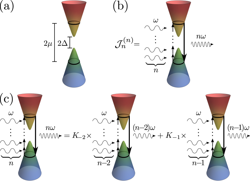
Figure 1: Diagrammatic representation of the band structure (a), of the $n^{\mathrm{th}}$ harmonic integrand $\mathcal{J}_{n}^{(n)}$ at the resonance $2\mu=n\omega$ (b) and of the iterative solution for $\mathcal{J}_{n}^{(n)}$ integrand (for $n^{\mathrm{th}}$ harmonic) as in Eq. (7). Here, $\mathcal{J}_{n}^{(n)}$ represents absorption of $n$ photons with frequency $\omega$, followed by the emission of a single photon with frequency $n\omega$.

To apply the iterative solution for $\mathcal{J}_{n}^{(j)}$ in practice, two seeds $\mathcal{J}_{0}^{(0)}$ and $\mathcal{J}_{1}^{(1)}$ are required that can easily be determined from low-order terms in Eq. (5). Collecting all terms independent of the external field and making use of the equilibrium charge distribution $\mathcal{N}_{0}=f_{1}-f_{2}$ (the difference between Fermi functions), the first seed reads $\mathcal{J}_{0}^{(0)}=F\mathcal{N}_{0}$. The second seed involves the collection of linear terms in the external field and reads $\mathcal{J}_{1}^{(1)}=2i\epsilon|G|^{2}\mathcal{N}_{0}\mathcal{A}_{0}/[4\epsilon^{2}-\omega^{2}]$. All remaining terms of $\mathcal{J}_{n}^{(j)}$ can be computed sequentially by evaluating all possible Fourier components $n=\{0,1,\ldots,j\}$, in increasing order, for any given response order $j$ using Eq. (Iterative approach to arbitrary nonlinear optical response functions of graphene). The solutions for all nonzero integrands up to fifth order are listed in this order in Tab. 1.

Table 1: Analytic expressions for current density integrands up to fifth order, where $\mathcal{J}_{n}^{(j)}\equiv\mathcal{F}_{n}^{(j)}|G|^{2}\mathcal{N}_{0}\mathcal{A}_{0}^{j}$.

$(n,j)$	$\mathcal{F}_{n}^{(j)}$
$(0,0)$	$F/|G|^{2}$
$(1,1)$	$2i\epsilon\big{/}[(4\epsilon^{2}-\omega^{2})]$
$(0,2)$	$-2F\big{/}[4\epsilon^{2}-\omega^{2}]$
$(2,2)$	$6\epsilon^{2}F\big{/}\big{[}(4\epsilon^{2}-4\omega^{2})(4\epsilon^{2}-\omega^{2})\big{]}$
$(1,3)$	$4i\epsilon\big{[}(13F^{2}-1)\epsilon^{2}-(4F^{2}-1)\omega^{2}\big{]}\big{/}\big{[}(4\epsilon^{2}-4\omega^{2})(4\epsilon^{2}-\omega^{2})^{2}\big{]}$
$(3,3)$	$-4i\epsilon\big{[}(5F^{2}-1)\epsilon^{2}+\omega^{2}\big{]}\big{/}\big{[}(4\epsilon^{2}-9\omega^{2})(4\epsilon^{2}-4\omega^{2})(4\epsilon^{2}-\omega^{2})\big{]}$
$(0,4)$	$-2F\big{[}2(13F^{2}-7)\epsilon^{2}-(8F^{2}-5)\omega^{2}\big{]}\big{/}\big{[}(4\epsilon^{2}-4\omega^{2})(4\epsilon^{2}-\omega^{2})^{2}\big{]}$
$(2,4)$	$16\epsilon^{2}F\big{[}8(8F^{2}-3)\epsilon^{4}-2(53F^{2}-28)\epsilon^{2}\omega^{2}+(27F^{2}-17)\omega^{4}\big{]}\big{/}\big{[}(4\epsilon^{2}-9\omega^{2})(4\epsilon^{2}-4\omega^{2})^{2}(4\epsilon^{2}-\omega^{2})^{2}\big{]}$
$(4,4)$	$-10\epsilon^{2}F\big{[}(7F^{2}-3)\epsilon^{2}+5\omega^{2}\big{]}\big{/}\big{[}8(4\epsilon^{2}-16\omega^{2})(4\epsilon^{2}-9\omega^{2})(4\epsilon^{2}-4\omega^{2})(4\epsilon^{2}-\omega^{2})\big{]}$
$(1,5)$	$48i\epsilon\big{[}8(61F^{4}-32F^{2}+1)\epsilon^{6}-2(503F^{4}-334F^{2}+11)\epsilon^{4}\omega^{2}+5(100F^{4}-77F^{2}+4)\epsilon^{2}\omega^{4}$
	$-3(24F^{4}-21F^{2}+2)\omega^{6}\big{]}\big{/}\big{[}(4\epsilon^{2}-9\omega^{2})(4\epsilon^{2}-4\omega^{2})^{2}(4\epsilon^{2}-\omega^{2})^{3}\big{]}$
$(3,5)$	$-16i\epsilon\big{[}4(295F^{4}-186F^{2}+11)\epsilon^{8}-(5235F^{4}-4166F^{2}+291)\epsilon^{6}\omega^{2}+(6095F^{4}-6303F^{2}+558)\epsilon^{4}\omega^{4}-(1440F^{4}$
	$-2569F^{2}+419)\epsilon^{2}\omega^{6}+36(3-8F^{2})\omega^{8}\big{]}\big{/}\big{[}(4\epsilon^{2}-16\omega^{2})(4\epsilon^{2}-4\omega^{2})^{2}(4\epsilon^{2}-9\omega^{2})^{2}(4\epsilon^{2}-\omega^{2})^{2}\big{]}$
$(5,5)$	$12i\epsilon\big{[}(21F^{4}-14F^{2}+1)\epsilon^{4}-5(1-7F^{2})\epsilon^{2}\omega^{2}+4\omega^{4}\big{]}\big{/}\big{[}(4\epsilon^{2}-25\omega^{2})(4\epsilon^{2}-16\omega^{2})(4\epsilon^{2}-9\omega^{2})(4\epsilon^{2}-4\omega^{2})(4\epsilon^{2}-\omega^{2})\big{]}$

The final response functions are obtained by integrating the desired $\mathcal{J}_{n}^{(j)}$ over $\kappa$-space and the respective conductivities $\sigma_{n}^{(j)}(\omega)$ then follow by writing

$$j(t)=\sum_{n,j}\big{[}\sigma_{n}^{(j)}(\omega)\mathcal{E}_{0}^{j}e^{-in\omega t}+\mathrm{c.c.}\big{]}/2.$$ (8)

In most cases, the integration is straightforward, but can lead to cumbersome expressions, particularly whenever the difference between the Fourier $n$ and response order $j$ is large. The angular part of the integral depends exclusively on powers of $F$ and $|G|$, therefore it can be shown that due to the presence of full rotation symmetry in the effective Hamiltonian all even-order response functions vanish upon angular integration. Nonetheless, even-order integrands remains necessary to determine higher order non-vanishing odd integrands.

Now, we turn our attention to the conductivities computed within the iterative framework. At low temperatures the population difference becomes a step function $\mathcal{N}_{0}=-\Theta(\epsilon-|\mu|)$ and the lower limit $\Omega$ of the radial part of the integral is determined by the larger of the Fermi level and mass term, i.e. $\Omega\equiv\max(|\mu|,\Delta)$ . In our explicit examples, we compute all conductivities up to ninth order Note (1). Among these, we examine in detail third and fifth harmonic generation as well as intensity-dependent refraction through the optical Kerr effect including high-order terms. As demonstrated in recent experiments Soavi et al. (2018); Jiang et al. (2018); Zhang et al. (2018), valuable information can be extracted by varying the Fermi level via electrostatic gating. Hence, we apply the present results to study the doping dependence of these NLO processes.

The third harmonic generation (THG) conductivity reads

$$\sigma_{3}^{(3)}(\omega) =\frac{-3i\sigma_{3}}{1024\pi}\bigg{(}\frac{2v_{F}}{3a_{0}\omega}\bigg{)}^{4}$$

$$\bigg{[}\bigg{(}45+\frac{56\Delta^{2}}{\omega^{2}}-\frac{48\Delta^{4}}{\omega^{4}}\bigg{)}\ln\frac{2\Omega-3\omega}{2\Omega+3\omega}$$

$$-\bigg{(}64+\frac{128\Delta^{2}}{\omega^{2}}-\frac{192\Delta^{4}}{\omega^{4}}\bigg{)}\ln\frac{2\Omega-2\omega}{2\Omega+2\omega}$$

$$+\bigg{(}17+\frac{88\Delta^{2}}{\omega^{2}}-\frac{240\Delta^{4}}{\omega^{4}}\bigg{)}\ln\frac{2\Omega-\omega}{2\Omega+\omega}\bigg{]},$$ (9)

where we define the scale of the 2D nonlinear conductivities systematically by $\sigma_{j>1}\equiv 2[3ea_{0}^{2}/(4\hbar v_{F})]^{j-1}\sigma_{1}$ with $\sigma_{1}=e^{2}/(4\hbar)$ and the carbon-carbon distance $a_{0}\equiv 1.42$ Å sets the natural length scale for graphene. Throughout the letter, we consider exclusively electron doping $\mu>0$, but results for hole doping $\mu<0$ simply follow by replacing $\mu\to-\mu$. Taking the limit $\Delta\to 0$, one can verify that our expression reduces to previous results derived with the gapless Dirac Hamiltonian using velocity and length gauges Cheng et al. (2014); Rostami and Polini (2016); Hipolito et al. (2018). The expression for $\sigma_{3}^{(3)}(\omega)$ is representative of the HHG conductivities, $\sigma_{n}^{(n)}(\omega)$, which are always composed by $n$ logarithmic divergences, whose amplitude is set by a polynomial prefactor with even powers of $\Delta/\omega$ as shown in Eq. S1a (see supplemental material). Note that the divergences found in the expressions are regularized by introducing a small broadening parameter $\omega\to\omega+i\eta$ and, unless stated otherwise, we use $\hbar\eta=1$ meV. The THG conductivities for both gapped and gapless graphene assuming photon energies in the low and medium range are shown in Fig. 2. Given the rather small gaps that can be reliably generated in graphene Zhou et al. (2007); Woods et al. (2014) (we take $E_{g}\equiv 250$ meV as a reference figure for our calculations) and considering photon energies $\hbar\omega>150$ meV, our results show that the response of gapless and gapped systems are generally similar but deviate whenever $\mu\lesssim\Delta$.

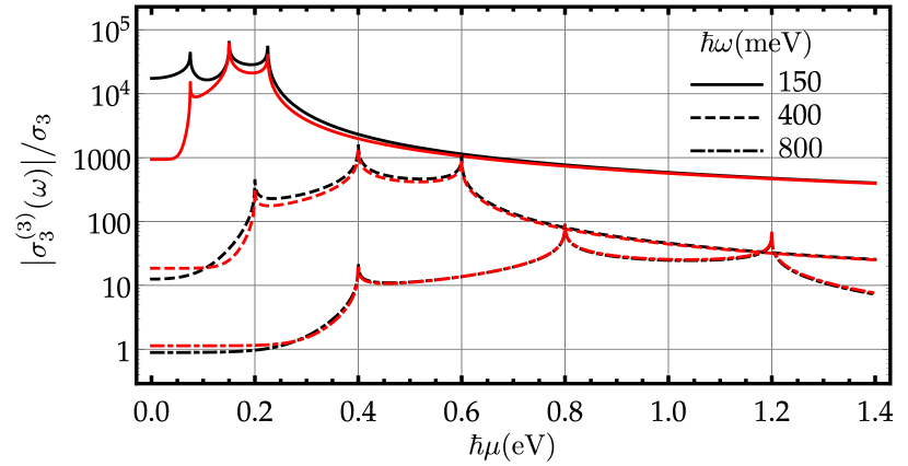
Figure 2: THG conductivity in gapped ($E_{g}=250$ meV, black) and gapless (red) graphene at photon energies $\hbar\omega=\{150,400,800\}$ meV.

The fifth harmonic conductivity in gapless graphene also lends itself to a closed form expression Note (1), with $n=5$ logarithmic divergences

$$\sigma_{5}^{(5)}(\omega) =\frac{9i\sigma_{5}}{655360\pi}\bigg{(}\frac{2v_{F}}{3a_{0}\omega}\bigg{)}^{8}\bigg{[}4925\ln\frac{2\mu-5\omega}{2\mu+5\omega}$$

$$-16384\ln\frac{2\mu-4\omega}{2\mu+4\omega}+19359\ln\frac{2\mu-3\omega}{2\mu+3\omega}$$

$$-9216\ln\frac{2\mu-2\omega}{2\mu+2\omega}+1266\ln\frac{2\mu-\omega}{2\mu+\omega}\bigg{]},$$ (10)

where the general expression valid for $\Delta\neq 0$ is given in Eq. (S3) Note (1). The fifth-order response of graphene is highly sensitive to the ratio between photon energy and doping level. This is illustrated in the contour plot in Fig. 3 of the amplitude of the fifth harmonic conductivity as function of these parameters. It shows that this response function can be tuned over several orders of magnitude by tuning either parameter, while highlighting the five resonances present in the fifth harmonic response. Moreover, we find that the nonlinear conductivities of graphene are regular in the limit of vanishing doping $\mu\to 0$

$$\lim_{\mu\to 0}\sigma_{n}^{(j)}/\sigma_{j}=q_{nj}\big{[}2v_{F}/(3a_{0}\omega)\big{]}^{2(j-1)}\,,$$ (11)

where the coefficients $q_{nj}$ are rational numbers. The complete list for all coefficients is found in Tab. S1 in supplemental material. For third and fifth harmonic generation, the coefficients read $q_{33}=3/512$ and $q_{55}=-45/65536$, respectively.

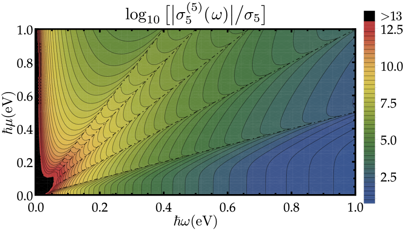
Figure 3: Contour plot of fifth harmonic conductivity in graphene. Dot-dashed lines show the resonant conditions $\mu=m\omega/2\,,m=\{1,2,3,4,5\}$ and the conductivity in the black region exceeds $10^{13}\sigma_{5}$.

The iterative approach can also readily be used to evaluate conductivities beyond harmonic generation such as the optical Kerr conductivity of graphene Note (1)

$$\sigma_{1}^{(3)}(\omega) =\frac{9i\sigma_{3}}{256\pi}\bigg{(}\frac{2v_{F}}{3a_{0}\omega}\bigg{)}^{4}\bigg{[}\frac{12\mu\omega}{4\mu^{2}-\omega^{2}}$$

$$-11\ln\frac{\omega-2\mu}{\omega+2\mu}+16\ln\frac{2\omega-2\mu}{2\omega+2\mu}\bigg{]}.$$ (12)

This expression is representative of high-order contributions to any Fourier order $\sigma_{n}^{(j>n)}$ Note (1). These expressions contain $(j+n)/2$ logarithmic divergences, rather than $j=n$ found in the $n^{\mathrm{th}}$ harmonic conductivities, and also contain an additional rational function with $(j+n-2)/2$ polynomial divergences that strongly enhance the nonlinear resonances, see Fig. S1 in supplemental material. In Fig. 4, we show the conductivities $\sigma_{1}^{(j)}$ contributing to the first harmonic current in doped graphene up to ninth order at $\mathcal{E}_{0}=2\,\mathrm{V/\mu m}$. Note that the field intensity considered in Fig. 4 matches the upper limit of the perturbative regime when considering THz radiation Hafez et al. (2018). Inspection of Fig. 4 defines the regime, where the perturbative approach breaks down, namely the frequency range, in which terms $\sigma_{1}^{(j)}\mathcal{E}_{0}^{j-1}$ cease to decrease as the order $j$ is increased. Hence, for the parameters in Fig. 4 the non-perturbative region can be estimated as $\hbar\omega\lesssim 60$ meV. Manifestations from higher than Kerr terms should be detectable as higher order terms introduce additional resonances that are highly sensitive to both the Fermi level and the magnitude of the external field.

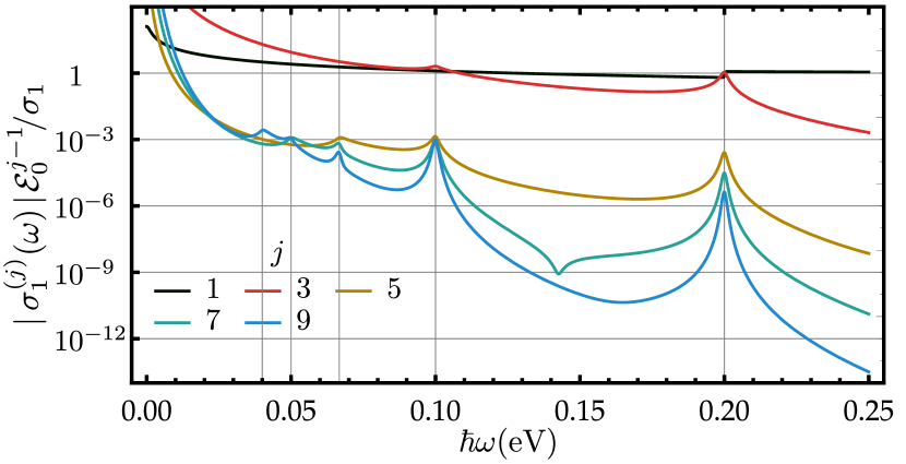
Figure 4: Linear and nonlinear contributions to the optical conductivity in doped graphene $\hbar\mu=100\,\mathrm{meV}$ at $\mathcal{E}_{0}=2\,\mathrm{V/\mu m}$. The black curve is the linear response and colored lines represent the nonlinearities. Vertical grid lines represent the $(n+j)/2$ resonances found in the nonlinear conductivities.

In Fig. 5, we plot the relative amplitude of the Fourier components of the radiated intensity $I_{n}(\omega)=\mu_{0}c|j_{n}(\omega)|^{2}/8$ with $j_{n}(\omega)=\sum_{j}\sigma_{n}^{(j)}(\omega)\mathcal{E}_{0}^{j}$ with respect to the incident intensity in vacuum $I_{0}=\varepsilon_{0}c_{0}\mathcal{E}_{0}^{2}/2$ Stauber et al. (2008); Hipolito and Pereira (2017) considering all contributions up to $j=15$. Note that the analytic expressions for the conductivities are limited to ninth order, hence all data plotted in Fig. 5 were integrated numerically using $\hbar\eta=10$ meV. Results shown in Figs. 2 to 5 demonstrate that the approach presented in this letter can be used to readily characterize harmonic response of graphene, including the effects from higher order terms, at arbitrary doping level and photon frequency, without requiring the complex numerical calculations found in time-dependent techniques.

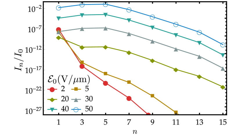
Figure 5: Intensity of HHG Fourier components in doped graphene ($\hbar\mu=250$ meV) normalized by $I_{0}=\varepsilon_{0}c_{0}\mathcal{E}_{0}^{2}/2$. The incident photon energy is $\hbar\omega=100$ meV and colors red to blue represent increasing field strengths.

In summary, we introduce and apply an iterative approach to the calculation of NLO response of systems described by the massive Dirac Hamiltonian. The iterative nature allows for analytical evaluation of high-order response functions, and we derive for the first time all nonlinear conductivities of (gapped) graphene up to ninth order. The NLO response of doped graphene reveals an intricate interplay between doping, photon energy and the intensity of the external electric field.