Consistent Skyrme parametrizations constrained by GW170817

Abstract

The high-density behavior of the stellar matter composed of nucleons and leptons under $\beta$ equilibrium and charge neutrality conditions is studied with the Skyrme parametrizations shown to be consistent (CSkP) with the nuclear matter, pure neutron matter, symmetry energy and its derivatives in a set of $11$ constraints [Dutra et al., Phys. Rev. C 85, 035201 (2012)]. The predictions of these parametrizations on the tidal deformabilities related to the GW170817 event are also examined. The CSkP that produce massive neutron stars give a range of $11.86~{}\mbox{km}\leqslant R_{1.4}\leqslant 12.55~{}\mbox{km}$ for the canonical star radius, in agreement with other theoretical predictions. It is shown that the CSkP are compatible with the region of masses and radii obtained from the analysis of recent data from LIGO and Virgo Collaboration (LVC). A correlation between dimensionless tidal deformability and radius of the canonical star is found, namely, $\Lambda_{1.4}\approx 3.16\times 10^{-6}R_{1.4}^{7.35}$, with results for the CSkP compatible with the recent range of $\Lambda_{1.4}=190_{-120}^{+390}$ from LVC. An analysis of the $\Lambda_{1}\times\Lambda_{2}$ graph shows that all the CSkP are compatible with the recent bounds obtained by LVC. Finally, the universal correlation between the moment of inertia and the deformability of a neutron star, named as the $I$-Love relation, is verified for the CSkP, that are also shown to be consistent with the prediction for the moment of inertia of the PSR J0737-3039 primary component pulsar.

I Introduction

Neutron stars are incredible natural laboratories for the study of nuclear matter at extreme conditions of isospin asymmetry and density ($\rho$) latt04 ; ozel06 . The properties of nuclear matter at such high densities are mostly governed by the equation(s) of state (EOS), which correlates pressure ($p$), energy density ($\epsilon$) and other thermodynamical quantities. From the terrestrial experiments, nuclear matter properties are mostly constrained up to saturation density, $\rho_{0}\approx 0.15$ fm${}^{-3}\approx 2.8\times 10^{14}$ g/cm³ tsan12 ; bald16 ; latt16 ; oert17 . The EOS correlating $p$, $\epsilon$ and $\rho$ is the sole ingredient to determine the relationship between the mass and radius of a neutron star by using the Tolman-Oppenheimer-Volkoff equations tov39 ; tov39a . It also plays a vital role in determining other star properties such as the moment of inertia and tidal deformability tanj10 ; phil18 . These last two quantities are shown to be correlated according to the so called $I$-Love relation phil18 ; science . The measurements of the neutron star spin, radius, and gravitational redshift provide weak constraints on the EOS as these measurements depend on the detailed modeling of the radiation mechanism and are subjected to a lot of systematic errors latt07 ; joce09 . However,the recent observation of the gravitational waves (GW) emission from the first binary neutron stars merger event, GW170817, provided new expectations to constrain the EOS in more efficient ways ligo17 ; ligo18 .

Since 2015, the observation of the GW emission from the binary compact objects, by LIGO aasi15 and Virgo acer15 collaborations, opened a platform to study the GW and related physics in more adequate ways. The GW170817 event, observed on 17 August 2017, has a special importance in nuclear physics since it consists of the emergence of GW from a binary system of neutron stars. It coincides with the detection of the $\gamma$-ray burst GRB170817 abbo17 ; gold17 and the components were verified as neutron stars by various electromagnetic spectrum observations abbo17a ; coul17 ; troj17 ; hagg17 ; hall17 . Hence, the GW170817 offers an opportunity to constrain the EOS from the tidal deformability data bhar17 ; tanj10 ; hind08 ; thib09 ; tayl09 , which establishes a relation between the internal structure of the neutron star and the emitted GW.

In the present context, we use the Skyrme model skyr61 ; vautherin ; bend03 ; ston07 in order to explore the possible constraints on the EOS by the observation of the GW170817 event. In the work of Ref. dutra12 , the authors have studied the nuclear matter characteristics of symmetric and asymmetric matter at saturation as well as at high densities by using $240$ parametrizations of the Skyrme energy density functional. Following this work, it was observed that $16$ parametrizations, namely, GSkI agrawal2006 , GSkII agrawal2006 , KDE0v1 agrawal2005 , LNS cao2006 , MSL0 chen2010 , NRAPR steiner2005 , Ska25s20 private2 , Ska35s20 private2 , SKRA rashdan2000 , Skxs20 brown2007 , SQMC650 guichon2006 , SQMC700 guichon2006 , SkT1 tondeur1984 ; stone2003 , SkT2 tondeur1984 ; stone2003 , SkT3 tondeur1984 ; stone2003 and SV-sym32 klupfel2009 , satisfy all the chosen $11$ constraints analyzed in Ref. dutra12 from symmetric nuclear matter, pure neutron matter, and a mixture of both related with the symmetry energy and its derivatives bianca . This set was named as Consistent Skyrme Parametrizations (CSkP), which is used in the present manuscript. These parametrizations offer a predictive power starting from sub-saturation density to very high density at very high isospin asymmetry, what has motivated us to analyze the stellar matter behavior for the CSkP, in particular, the tidal deformability related to the GW170817 event.

We point out that the constraints analyzed in Ref. dutra12 were chosen by collecting previous existing constraints in the literature at the time. In that sense, they are not unique and can be subject to improvements and/or updates. Actually, in subsequent works, relativistc mean-field models were analyzed by a set of updated constraints  rmf ; rmfdef in comparison with those used in Ref. dutra12 . However, we also remark here that the main purpose of the paper in Ref. dutra12 was to establish some general criteria and analyse the models according to them. The purpose of the present paper is not to justify the criteria chosen in Ref. dutra12 , but to use the models consistent with all those chosen constraints to verify whether (or not) they could also satisfy the new constraints imposed by the GW170817 event.

We try to correlate the tidal deformability of the canonical neutron star ($\Lambda_{1.4}$) and the corresponding radius ($R_{1.4}$) for the CSkP by addressing a transparent relation between $\Lambda_{1.4}$ and $R_{1.4}$ as a power law. Usually, the proportionality relation $\Lambda\propto R^{5}$, which is based on the definition $\Lambda=(2/3)k_{2}(R/M)^{5}$, with $M$ being the neutron star mass, is cited in the literature. It is worth noticing that this proportionality is not exact since the Love number $k_{2}$ depends on the radius $R$ through a complicated second order differential equation. In recent studies, various relations between the $\Lambda_{1.4}$ and $R_{1.4}$ are obtained with different models, like the Skyrme malik18 and relativistic mean-field fatt18 ones. Here, we study this correlation with CSkP. The predictions of the CSkP regarding the values for $\Lambda_{1.4}$ and the tidal deformabilities of the binary neutron star system, namely, $\Lambda_{1}$ and $\Lambda_{2}$ are also presented. The verification of the $I$-Love relation, and the predictions for the dimensionless moment of inertia of the PSR J0737-3039 primary component pulsar, obtained from the CSkP, are also performed.

This manuscript is organized as follows. In Sec. II, we briefly outline the theoretical formalism of the Skyrme model in nuclear and neutron star matter. In Sec. III, we discuss the predictions of CSkP concerning the recent constraints obtained from the GW170817 event and verify the $I$-Love relation. Special attention is given to the tidal deformability of the neutron stars binary system. We conclude the manuscript with a brief summary in Sec. IV.

II Theoretical Formalism

II.1 Infinite nuclear matter

In the following, we mention the EOS used in this work related to the Skyrme model at zero temperature. The energy density of infinite nuclear matter, defined in terms of the density and proton fraction, is written as dutra12

$$\epsilon(\rho,y_{p}) =\frac{3\hbar^{2}}{10M_{\rm nuc}}\left(\frac{3\pi^{2}}{2}\right)^{2/3}\rho^{5/3}H_{5/3}(y_{p})$$

$$+\frac{t_{0}}{8}\rho^{2}[2(x_{0}+2)-(2x_{0}+1)H_{2}(y_{p})]$$

$$+\frac{1}{48}\sum_{i=1}^{3}t_{3i}\rho^{\sigma_{i}+2}[2(x_{3i}+2)-(2x_{3i}+1)H_{2}(y_{p})]$$

$$+\frac{3}{40}\left(\frac{3\pi^{2}}{2}\right)^{2/3}\rho^{8/3}[aH_{5/3}(y_{p})+bH_{8/3}(y_{p})],$$ (1)

with

$$a = t_{1}(x_{1}+2)+t_{2}(x_{2}+2),$$ (2)

$$b = \frac{1}{2}\left[t_{2}(2x_{2}+1)-t_{1}(2x_{1}+1)\right],$$ (3)

and

$$H_{l}(y_{p}) = 2^{l-1}[y_{p}^{l}+(1-y_{p})^{l}],$$ (4)

where $y_{p}=\rho_{p}/\rho$ is the proton fraction, and $M_{\rm nuc}c^{2}=939$ MeV is the nucleon rest mass, assumed equal for protons and neutrons. A particular parametrization is defined by a specific set of the following free parameters: $x_{0}$, $x_{1}$, $x_{2}$, $x_{31}$, $x_{32}$, $x_{33}$, $t_{0}$, $t_{1}$, $t_{2}$, $t_{31}$, $t_{32}$, $t_{33}$, $\sigma_{1}$, $\sigma_{2}$, and $\sigma_{3}$.

From Eq. (1), one can construct the pressure of the model as

$$p(\rho,y_{p})=\rho^{2}\frac{\partial(\mathcal{E}/\rho)}{\partial\rho}=\frac{\hbar^{2}}{5M_{\rm nuc}}\left(\frac{3\pi^{2}}{2}\right)^{2/3}\rho^{5/3}H_{5/3}(y_{p})$$

$$+\frac{t_{0}}{8}\rho^{2}[2(x_{0}+2)-(2x_{0}+1)H_{2}(y_{p})]$$

$$+\frac{1}{48}\sum_{i=1}^{3}t_{3i}(\sigma_{i}+1)\rho^{\sigma_{i}+2}[2(x_{3i}+2)-(2x_{3i}+1)H_{2}(y_{p})]$$

$$+\frac{1}{8}\left(\frac{3\pi^{2}}{2}\right)^{2/3}\rho^{8/3}[aH_{5/3}(y_{p})+bH_{8/3}(y_{p})].$$ (5)

Notice that pressure and energy density are given in units of MeV/fm³ and can be converted into units of fm^-4 by using the following conversion factor: $1$ fm${}^{-4}=197.33$ MeV/fm³. The nucleon chemical potential is given by

$$\mu_{q}(\rho,y_{p})=\frac{\partial\epsilon}{\partial\rho_{q}}=\frac{\hbar^{2}}{2M_{\rm nuc}}\left(\frac{3\pi^{2}}{2}\right)^{2/3}\rho^{2/3}H_{5/3}(y_{p})$$

$$+\frac{1}{5}\left(\frac{3\pi^{2}}{2}\right)^{2/3}\rho^{5/3}[aH_{5/3}(y_{p})+bH_{8/3}(y_{p})]$$

$$+\frac{t_{0}}{4}\rho[2(x_{0}+2)-(2x_{0}+1)H_{2}(y_{p})]$$

$$+\frac{1}{48}\sum_{i=1}^{3}t_{3i}(\sigma_{i}+2)\rho^{\sigma_{i}+1}[2(x_{3i}+2)-(2x_{3i}+1)H_{2}(y_{p})]$$

$$\pm\frac{1}{2}\left[1\mp(2y_{p}-1)\right]\left\{\frac{3\hbar^{2}}{10M_{\rm nuc}}\left(\frac{3\pi^{2}}{2}\right)^{2/3}\rho^{2/3}H^{\prime}_{5/3}(y_{p})\right.$$

$$\left.-\frac{t_{0}}{8}\rho(2x_{0}+1)H^{\prime}_{2}(y_{p})-\frac{1}{48}\sum_{i=1}^{3}t_{3i}\rho^{\sigma_{i}+1}(2x_{3i}+1)H^{\prime}_{2}(y_{p})\right.$$

$$+\left.\frac{3}{40}\left(\frac{3\pi^{2}}{2}\right)^{2/3}\rho^{5/3}[aH^{\prime}_{5/3}(y_{p})+bH^{\prime}_{8/3}(y_{p})]\right\},$$ (6)

where $q=p,n$ stands for protons and neutrons, respectively. Here one also has that $H^{\prime}_{l}(y_{p})=dH_{l}/dy_{p}$.

II.2 Neutron star matter

For a correct treatment of the stellar matter, one needs to implement charge neutrality and $\beta$-equilibrium conditions under the weak processes, $n\rightarrow p+e^{-}+\bar{\nu}_{e}$, and its inverse process $p+e^{-}\rightarrow n+\nu_{e}$. For densities in which $\mu_{e}$ exceeds the muon mass, the reactions $e^{-}\rightarrow\mu^{-}+\nu_{e}+\bar{\nu}_{\mu}$, $p+\mu^{-}\rightarrow n+\nu_{\mu}$, and $n\rightarrow p+\mu^{-}+\bar{\nu}_{\mu}$ energetically favor the emergence of muons. Here, we consider that neutrinos are able to escape the star due to their extremely small cross-sections at zero temperature. By taking these assumptions into account, we can write the total energy density and pressure of the stellar system for the Skyrme model, respectively, as

$$\mathcal{E}(\rho,\rho_{e},y_{p}) =\epsilon(\rho,y_{p})+\frac{\mu_{e}^{4}(\rho_{e})}{4\pi^{2}\hbar^{3}c^{3}}+M_{\rm nuc}c^{2}\rho$$

$$+\frac{1}{\pi^{2}\hbar^{3}c^{3}}\int_{0}^{\sqrt{\mu_{\mu}^{2}(\rho_{e})-m^{2}_{\mu}c^{4}}}dk\,k^{2}(k^{2}+m_{\mu}^{2}c^{4})^{1/2},$$ (7)

and

$$P(\rho,\rho_{e},y_{p}) =p(\rho,y_{p})+\frac{\mu_{e}^{4}(\rho_{e})}{12\pi^{2}\hbar^{3}c^{3}}$$

$$+\frac{1}{3\pi^{2}\hbar^{3}c^{3}}\int_{0}^{\sqrt{\mu_{\mu}^{2}(\rho_{e})-m^{2}_{\mu}c^{4}}}\frac{dk\,k^{4}}{(k^{2}+m_{\mu}^{2}c^{4})^{1/2}},$$ (8)

where, $\epsilon(\rho,y_{p})$ and $p(\rho,y_{p})$ are given in the Eqs. (1) and (5), respectively. The chemical equilibrium and the charge neutrality conditions are

$$\mu_{n}(\rho,y_{p})-\mu_{p}(\rho,y_{p})=\mu_{e}(\rho_{e}),$$ (9)

and

$$\rho_{p}(\rho,y_{p})-\rho_{e}=\rho_{\mu}(\rho_{e}),$$ (10)

where $\mu_{p}$ and $\mu_{n}$ are found from Eq. (6), $\mu_{e}=\hbar c(3\pi^{2}\rho_{e})^{1/3}$, $\rho_{p}=y_{p}\rho$, $\rho_{\mu}=[(\mu_{\mu}^{2}-m_{\mu}^{2})^{3/2}]/(3\pi^{2}\hbar^{3}c^{3})$, and $\mu_{\mu}=\mu_{e}$, for $m_{\mu}c^{2}=105.7$ MeV and massless electrons (the ultrarelativistic limit is a suitable assumption here since the electron rest mass is around $0.5$ MeV). Regarding the muons, their energy density and pressure are given by the last terms of Eqs. (7) and (8), respectively, with the degeneracy factor equal to $2$. Thus, for each input density $\rho$, the quantities $\rho_{e}$ and $y_{p}$ are calculated by simultaneously solving conditions (9) and (10), along with the definitions of $\rho_{\mu}$ and $\mu_{\mu}$ (both functions of $\rho_{e}$) previously given in the text.

The properties of a spherically symmetric static neutron star can be studied by taking the energy density and pressure as input to the widely known TOV equations, which are given by tov39 ; tov39a ,

$$\dfrac{dP(r)}{dr} = -\dfrac{\left[{\mathcal{E}}(r)+P(r)\right]\left[m(r)+4\pi r^{3}P(r)\right]}{r^{2}\left[1-\dfrac{2m(r)}{r}\right]}$$

and

$$\dfrac{dm(r)}{dr} = 4\pi r^{2}{\mathcal{E}}(r),$$ (12)

where the solution is constrained to the following two conditions at the neutron star center: $P(0)=P_{c}$ (central pressure), and $m(0)=0$ (central mass). Furthermore, at the star surface one has $P(R)=0$ and $m(R)\equiv M$, with $R$ being the neutron star radius. These equations are given in gravitational units, in which $G=1=c$ glend . In this specific unit system, mass can be expressed in length units and density as inverse length square, as for example in km^-2. On the other hand, in natural units ($\hbar=c=1$), energy density and pressure can also be expressed in fm^-4, as stated immediately after Eq. (5). By mixing both, graviational and natural units, one finds $1$ fm${}^{-4}=2.6115\times 10^{-4}$ km^-2 glend that is used to express energy density and pressure in units of km^-2. In this case, mass and radius have the same unit, namely, km (with $1\,M_{\odot}=1.4766$ km glend ).

In order to solve the TOV equations in this work, we take $\mathcal{E}$ and $P$ given in Eqs. (7) and (8) as the EOS that describes the neutron star core. For the crust, we consider the different regions defined as the outer and the inner crust. We describe the outer crust by the EOS developed by Baym, Pethick and Sutherland (BPS) bps in a density region from $\rho=6.3\times 10^{-12}\,\mbox{fm}^{-3}$ to $\rho=2.5\times 10^{-4}\,\mbox{fm}^{-3}$. The exact range is not known, but the outer crust is estimated to exist at densities around $10^{4}$ g/cm³ to $4\times 10^{11}$ g/cm³, i.e, around $5\times 10^{-12}$ fm^-3 to $2\times 10^{-4}$ fm^-3, see Refs. bps ; poly2 , for instance. Our choice for this range is compatible with this estimation. A similar range was also used in Ref. malik19 . For the inner crust region, on the other hand, we impose a polytropic form for the total pressure as a function of the total energy density, namely, $P(\mathcal{E})=A+B\mathcal{E}^{4/3}$ poly2 ; poly1 ; gogny2 , from $\rho=2.5\times 10^{-4}\,\mbox{fm}^{-3}$ to $\rho=\rho_{t}$. Here, $\rho_{t}$ is related to the core-crust transition, in our case estimated from the thermodynamical method described in Refs. gogny1 ; cc2 ; gonzalez19 , for instance. Such a procedure establishes that the transition density is defined by the crossing of the EOS with the spinodal section, as one can see in Ref. debora06 . $A$ and $B$ are constants found by imposing the matching between the outer and the inner crust, and between the inner crust and the core. The EOS for the KDEv01 parametrization is shown in Fig. 1 and illustrates the piecewise structure we use in this work.

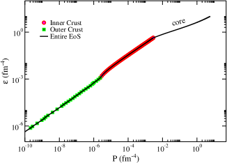
Figure 1: Neutron star matter EOS for the KDE0v1 parametrization.

The remaining CSkP follow the same pattern.

II.3 Tidal deformability and moment of inertia

In order to perform a detailed analysis concerning the prediction of the CSkP on the recent GW170817 event, a very important quantity has to be computed, namely, the tidal deformability. It is one of the observed quantities in the binary neutron stars system ligo17 ; ligo18 , which plays a major role in constraining hadronic EOS. The induced quadrupole moment $Q_{ij}$ in one neutron star of a binary system due to the static external tidal field $E_{ij}$ created by the companion star can be written as tanj10 ; hind08 ,

$$Q_{ij}=-\lambda{E}_{ij}.$$ (13)

Here, $\lambda$ is the tidal deformability parameter, which can be expressed in terms of dimensionless quadrupole tidal Love number $k_{2}$ as

$$\lambda=\frac{2}{3}{k_{2}}R^{5}.$$ (14)

The dimensionless tidal deformability $\Lambda$ (i.e., the dimensionless version of $\lambda$) is connected with the compactness parameter $C=M/R$ through

$$\Lambda=\frac{2k_{2}}{3C^{5}}.$$ (15)

The tidal Love number $k_{2}$ is obtained as

$$k_{2} =\frac{8C^{5}}{5}(1-2C)^{2}[2+2C(y_{R}-1)-y_{R}]$$

$$\times\Big{\{}2C[6-3y_{R}+3C(5y_{R}-8)]$$

$$+4C^{3}[13-11y_{R}+C(3y_{R}-2)+2C^{2}(1+y_{R})]$$

$$+3(1-2C)^{2}[2-y_{R}+2C(y_{R}-1)]{\rm ln}(1-2C)\Big{\}}^{-1},\,\,$$ (16)

with $y_{R}\equiv y(R)$, where $y(r)$ is found from the solution of

$$r\frac{dy}{dr}+y^{2}+yF(r)+r^{2}Q(r)=0,$$ (17)

with

$$F(r)=\frac{r-4\pi r^{3}[\mathcal{E}(r)-P(r)]}{r-2m(r)}$$ (18)

and

$$Q(r) =\frac{4\pi r\left[5\mathcal{E}(r)+9P(r)+\frac{\mathcal{E}(r)+P(r)}{\partial P(r)/\partial\mathcal{E}(r)}-\frac{6}{4\pi r^{2}}\right]}{r-2m(r)}$$

$$-4\left[\frac{m(r)+4\pi r^{3}P(r)}{r^{2}(1-2m(r)/r)}\right]^{2}.$$ (19)

In order to find $y(r)$, Eq. (17) has to be solved as part of a coupled system containing the TOV equations given in Eqs. (LABEL:tov1) and (12).

The dimensionless tidal deformabilities of a binary neutron stars system, namely, $\Lambda_{1}$ and $\Lambda_{2}$, can be combined to yield the weighted average as ligo17

$$\tilde{\Lambda}=\frac{16}{13}\frac{(m_{1}+12m_{2})m_{1}^{4}\Lambda_{1}+(m_{2}+12m_{1})m_{2}^{4}\Lambda_{2}}{(m_{1}+m_{2})^{5}},$$ (20)

where $m_{1}$ and $m_{2}$ are masses of the two companion stars.

Finally, in order to verify whether the $I$-Love relation also applies to the CSkP, we solve the Hartle’s slow rotation equation given in Refs. phil18 ; hartle ; yagi13 , namely,

$$0 = [r-2m(r)]\frac{d^{2}\omega}{dr^{2}}-16\pi r[\mathcal{E}(r)+P(r)]\omega(r)$$ (21)

$$+ 4\left\{\left(1-\frac{2m(r)}{r}\right)-\pi r^{2}[\mathcal{E}(r)+P(r)]\right\}\frac{d\omega}{dr},$$

coupled to the TOV equations. Since the binary system related to the GW170817 event rotates slowly, according to Ref. phil18 , the Hartle’s method can be safely used.

From the solution $\omega(r)$, one determines the moment of inertia through the relation $I=R^{3}(1-\omega_{R})/2$, with $\omega_{R}\equiv\omega(R)$. The dimensionless version of this quantity is defined as $\bar{I}\equiv I/M^{3}$. The linearized version of Eq. (21) is given by

$$r\frac{d\zeta}{dr}+\zeta\left(\zeta+3\right)-\frac{4\pi r^{2}[\mathcal{E}(r)+P(r)](\zeta+4)}{1-2m(r)/r}=0$$ (22)

with

$$\zeta\equiv\frac{1}{\omega}\frac{d\omega}{dr}.$$ (23)

In this case, the boundary conditions are $\zeta=0$ at the center, and $I=[\zeta/(3+\zeta)]R^{3}/2$ at the surface. This formulation is easier to be numerically integrated since it is a first-order differential equation.

III Results and Discussions

As all the CSkP come from a nonrelativistic mean field model, at zero temperature regime, the causal limit may be broken at the high density region, since the sound velocity ($v_{s}$) increases with density, or equivalently, with energy density. However, for the CSkP we verify that $v_{s}^{2}=\partial P/\partial\mathcal{E}$ exceeds $c^{2}=1$ only at very high energy density values, as we can see in Fig. 2.

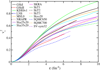
Figure 2: Squared sound velocity as a function of total energy density for the CSkP.

From this figure, one can verify that the CSkP obey the causal limit up to a range of $\mathcal{E}\lesssim 10$ fm^-4. By comparing these results with those obtained for relativistic mean-field (RMF) parametrizations in Fig. 2 of Ref. dutra16 , a clear difference in behavior is observed. The RMF parametrizations present a saturation for the sound velocity unlike the Skyrme ones, that always increase. Despite this increasing dependence, Fig. 2 shows that it is possible to describe neutron star matter with CSkP within a particular range of energy densities. The description of global properties of neutron stars by other different Skyrme parametrizations can be found, for instance, in Refs. phil18 ; malik18 ; sk1 ; sk2 ; sk3 ; sk4 ; sk5 ; sk6 . Notice that the curves that end below an energy density around 8 fm^-4 refer to models that stop converging at these lower densities. Had we plotted the sound velocity as a function of the baryonic density, the behavior would be similar. For all models, the baryonic density corresponding to the energy density equal to 2 (6) fm^-4 is of the order of 0.4 (1.0) fm^-3 and a ratio of 2.4 (6) times their saturation densities. Furthermore, other nonrelativistic models such as Gogny, Simple Effective Interaction (SEI), and momentum-dependent interaction (MDI), based on finite range interactions unlike the Skyrme model, are also used in neutron star calculations, see Refs. gogny2 ; gogny1 ; sei1 ; sei2 ; kras19 .

The mass-radius profiles predicted by the CSkP are shown in Fig. 3. In this figure, horizontal bands in magenta and green colors indicate respectively the observational data of pulsar masses of PSR J1614-2230 nature467-2010 and PSR J0348+0432 science340-2013 . We also show the empirical constraints for the mass-radius profile for the cold dense matter inside the neutron star. They were obtained from a Bayesian analysis of type-I x-ray burst observations by Nättilä, et al. in Ref. nat16 (outer orange and inner red bands), and from a mass-radius coming from six sources, namely, three from transient low-mass x-ray binaries and three from type-I x-ray bursts with photospheric radius expansion, by Steiner et al. in Ref. stein10 (outer white and inner black bands). In the same figure, it is also represented by the turquoise band the region of masses and radii obtained from the analysis of the GW170817 event regarding the binary neutron star system ligo18 .

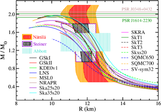
Figure 3: Neutron star mass-radius profiles for the CSkP. Horizontal bands indicate the masses of PSR J1614-2230 nature467-2010 and PSR J0348+0432 science340-2013 . Turquoise band: limits from the GW170817 event found in Ref. ligo18 .

These observations imply that the neutron star mass predicted by any theoretical model should reach the limit of $M\sim 2.0M_{\odot}$. From the results, we find that the maximum masses obtained by the GSkI, Ska35s20, MSL0, NRAPR, and KDE0v1 parametrizations are in agreement with at least one of these boundaries nature467-2010 ; science340-2013 . Very recently, another massive millisecond pulsar was confirmed, namely, MSP J0740+6620, with a mass of $2.14^{+0.20}_{-0.18}M_{\odot}$ within 95.4% credibility or $2.14^{+0.10}_{-0.09}M_{\odot}$ within 68.3% credibility nature_2019 . Indeed, four of the models mentioned above, namely, GSkI, Ska35s20, MSL0 and KDE0v1, also lie within the former mass limit of this pulsar ($2.14^{+0.20}_{-0.18}M_{\odot}$), as one can verify from the results presented in Table 1.

Table 1: Transitions values ($\rho_{t}$, $\epsilon_{t}$, and $p_{t}$) along with the stellar matter properties obtained from the CSkP: maximum neutron stars mass ($M_{\rm max}$) and its corresponding radius ($R_{\rm max}$), compactness ($C_{\rm max}$), and central energy density ($\mathcal{E}_{c}$) along with the radius ($R_{1.4}$) and compactness ($C_{1.4}$) of the canonical star.

Parameter	$\rho_{t}$	$\epsilon_{t}$	$p_{t}$	$M_{\rm max}$	$R_{\rm max}$	$C_{\rm max}$	$\mathcal{E}_{c}$	$R_{\rm 1.4}$	$C_{\rm 1.4}$
	(fm-3)	(fm-4)	(MeV/fm3)	($M_{\odot}$)	(${\rm km}$)	($M_{\odot}/{\rm km}$)	(${\rm fm}^{-4}$)	(${\rm km}$)	($M_{\odot}/{\rm km}$)
GSkI	0.081	0.390	0.492	1.974	10.229	0.193	8.095	12.419	0.113
GSkII	0.087	0.417	0.532	1.594	10.452	0.153	6.094	11.267	0.124
KDE0v1	0.089	0.429	0.570	1.970	9.863	0.200	8.573	11.858	0.118
LNS	0.087	0.417	0.612	1.728	9.436	0.183	9.848	11.278	0.124
MSL0	0.079	0.381	0.441	1.956	10.155	0.193	8.198	12.258	0.114
NRAPR	0.083	0.397	0.553	1.939	10.032	0.193	8.481	12.188	0.115
Ska25s20	0.083	0.399	0.577	1.859	9.981	0.186	8.711	12.112	0.116
Ska35s20	0.085	0.406	0.594	1.964	10.358	0.190	7.975	12.553	0.112
SkRA	0.083	0.398	0.529	1.774	9.643	0.184	9.332	11.599	0.121
SkT1	0.087	0.420	0.560	1.838	10.215	0.180	7.458	11.895	0.118
SkT2	0.087	0.419	0.560	1.837	10.210	0.180	7.467	11.892	0.118
SkT3	0.087	0.418	0.541	1.844	10.185	0.181	7.536	11.870	0.118
Skxs20	0.081	0.388	0.615	1.750	9.771	0.179	9.306	11.815	0.118
SQMC650	0.093	0.446	0.694	1.452	10.029	0.145	6.790	10.355	0.135
SQMC700	0.088	0.422	0.630	1.760	9.568	0.184	9.520	11.473	0.122
SV-sym32	0.085	0.410	0.589	1.696	10.490	0.162	6.760	11.819	0.118

Furthermore, the radii obtained from these parametrizations for the canonical star of $M=1.4M_{\odot}$ are also inside the bands calculated in Refs. nat16 ; stein10 . The remaining CSkP underestimate the observed data regarding the neutron star mass. Finally, concerning the GW170817 constraint, one can verify that all the CSkP are entirely compatible with this particular restriction. The exception is the SQMC650 parametrization, that satisfies the constraint only partially.

In Table 1 we also present some properties regarding the CSkP, namely, the transition point (transition density, energy density and pressure) found by the thermodynamical method gogny1 ; cc2 ; gonzalez19 , and neutron star matter quantities. For the latter, we show the maximum neutron star mass and corresponding radius, compactness and central energy density. We also tabulate the radius and compactness related to the canonical neutron star. It is worth mentioning that the central energy density of all CSkP are compatible with the causal limit, as one can verify from Fig. 2.

In the recent literature, a lot of effort has been put to constrain the radius of the canonical neutron star, see for instance, Refs. malik18 ; yeun18 ; elia18 ; zhan19 ; caro18 ; tews18 . In Ref. malik18 , Tuhin Malik et al. have discussed this constraint by using Skyrme and RMF models and their calculations suggest the range of $11.82~{}\mbox{km}\leqslant R_{1.4}\leqslant 13.72~{}\mbox{km}$. By using a set of more realistic models and the neutron skin values as a new constraint, F. J. Fattoyev et al. have shown the upper limit for $R_{1.4}$ as $13.76~{}\mbox{km}$ fatt18 . In Ref. yeun18 , Yeunhwan Lim et al. have used chiral effective field theory and constraints from nuclear experiments to establish the range of $10.36~{}\mbox{km}\leqslant R_{1.4}\leqslant 12.87~{}\mbox{km}$. Elias R. Most et al. have studied the constraint on $R_{1.4}$ with a large number of EOS with pure hadronic matter without any kind of phase transition elia18 . They found the value of $R_{1.4}$ inside the range of $12.00~{}\mbox{km}\leqslant R_{1.4}\leqslant 13.45~{}\mbox{km}$, with the most likely value of $R_{1.4}=12.39~{}\mbox{km}$. From the above discussion, we can estimate an specific range for $R_{1.4}$ encompassing the previous ones as $10.36~{}\mbox{km}\leqslant R_{1.4}\leqslant 13.76~{}\mbox{km}$. Our calculations for $R_{1.4}$ from the CSkP show a minimum value of 10.36 km (SQMC650 parametrization), while the maximum value is given by 12.55 km (Ska35s20 parameter set). Both maximum and minimum values present very good agreement with the composite range. As a consequence, the 5 CSkP predicting neutron star mass around two solar masses, namely, GSkI, KDE0v1, MSL0, NRAPR, and Ska35s20, also present $R_{1.4}$ compatible with the range mentioned above. The minimum value of this quantity is obtained by the KDE0v1 parametrization: $R_{1.4}=11.86$ km, while the maximum value is found by the Ska35s20 set, namely, $R_{1.4}=12.55$ km. This number is close to the most likely value of $R_{1.4}$ given in Ref. elia18 , namely, $R_{1.4}=12.39~{}\mbox{km}$.

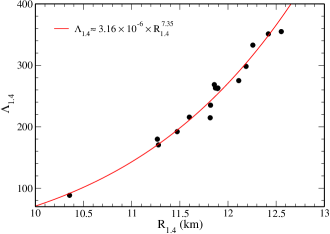
Figure 4: Canonical neutron star tidal deformability as a function of its radius for the CSkP. Solid line: fitting curve.

In searching for other possible correlations in the context of the neutron star binary system, one can notice from Eq. (15) that $\Lambda\propto R^{5}$ is not a good assumption, since the tidal Love number $k_{2}$ depends on the neutron star radius in a nontrivial way, as seen in Eq. (16). In this context, we try to find a correlation between the radius and tidal deformability for the CSkP for the canonical star, the one with $M=1.4M_{\odot}$. The obtained results for $\Lambda_{1.4}$ as a function of $R_{1.4}$ are shown in Fig. 4, with a similar qualitative behavior in comparison with the study performed in Ref. tsang , for instance. From the points shown in the figure, we could establish a fitting curve correlating $\Lambda_{1.4}$ as a function of $R_{1.4}$, namely, $\Lambda_{1.4}\approx 3.16\times 10^{-6}R_{1.4}^{7.35}$. This correlation presents different numbers in comparison with those found from predictions of EOS constructed by chiral effective field theory at low densities and the perturbative QCD at very high baryon densities using polytropes anna18 , several energy density functional within RMF models fatt18 , and both RMF and Skyrme Hartree-Fock energy density functionals malik18 . In these cited works, the authors found $\Lambda_{1.4}\approx 2.88\times 10^{-6}R_{1.4}^{7.5}$ anna18 , $\Lambda_{1.4}\approx 7.76\times 10^{-4}R_{1.4}^{5.28}$ fatt18 , and $\Lambda_{1.4}\approx 9.11\times 10^{-5}R_{1.4}^{6.13}$ malik18 . A recent analysis performed in Ref. rmfdef by using a set of consistent RMF parametrizations, pointed out to $\Lambda_{1.4}\approx 2.65\times 10^{-5}R_{1.4}^{6.58}$. These different fittings point towards the non-existence of an universal power-law of $\lambda$ or $\Lambda$ as a function of $R$, as one could naively think by looking at Eqs. (14) and (15).

For the sake of completeness, in Fig. 5 we plot the dimensionless tidal deformability $\Lambda$ of a static neutron star as a function of its mass for the CSkP. The tidal deformability decreases nonlinearly with the neutron star mass for all parametrizations. At $M=1.4M_{\odot}$, the resulting values of $\Lambda$ stand within a range of around $100-350$ for the CSkP, which are within the upper limit of $\Lambda_{1.4}\leqslant 800$ of LIGO + Virgo gravitational detection ligo17 , and also the recent updated range of $\Lambda_{1.4}=190_{-120}^{+390}$ ligo18 .

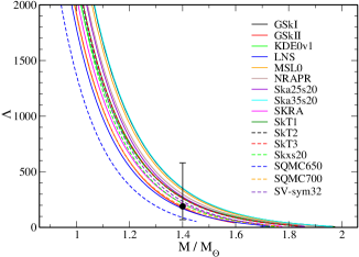
Figure 5: $\Lambda$ as a function of $M$ for the CSkP. Full circle: recent result of $\Lambda_{1.4}=190_{-120}^{+390}$ obtained by LIGO an Virgo Collaboration ligo18 related to the canonical star.

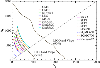
Figure 6: Tidal deformability parameters predicted by the CSkP for the case of high-mass ($\Lambda_{1}$) and low-mass ($\Lambda_{2}$) components of the observed GW170817 event. The 90% and 50% confidence lines were taken from recent findings of Ref. ligo18 .

In Fig. 6 we plot the tidal deformabilities $\Lambda_{1}$ and $\Lambda_{2}$ of the binary neutron stars system with component masses of $m_{1}$ and $m_{2}$ ($m_{1}>m_{2}$). The diagonal dotted line corresponds to the $\Lambda_{1}=\Lambda_{2}$ case in which $m_{1}=m_{2}$. The analysis takes into account the range for $m_{1}$ given by $1.365\leqslant m_{1}/M_{\odot}\leqslant 1.60$, as pointed out in Ref. ligo17 . The mass of the companion star, $m_{2}$, is calculated through the relationship between $m_{1}$, $m_{2}$ and the chirp mass given by

$$\mathcal{M}_{c}=\frac{(m_{1}m_{2})^{3/5}}{(m_{1}+m_{2})^{1/5}}.$$ (24)

In this equation, $\mathcal{M}_{c}$ is fixed at the observed value of $1.188M_{\odot}$ ligo17 . The upper and lower dash lines correspond to the 90% and 50% confidence limits respectively, which are obtained from the recent analysis of the GW170817 event ligo18 . This figure shows that all $16$ CSkP are completely inside the 90% credible region predicted by the GW170817 data ligo18 . Other kind of models, such as some relativistic ones rmfdef ; apj also present good agreement with this particular region predicted by the the LIGO and Virgo Collaboration.

We also calculate the ranges related to the mass weighted tidal deformability as defined in Eq. (20) by using $\mathcal{M}_{c}=1.188M_{\odot}$ and the aforementioned variations of $m_{1}$ and $m_{2}$. The results are presented in Table 2.

Table 2: Ranges for $\tilde{\Lambda}$ predicted by the CSkP.

Parameter	Range of $\tilde{\Lambda}$
GSkI	420 - 427
GSkII	224 - 238
KDE0v1	321 - 326
LNS	210 - 223
MSL0	398 - 406
NRAPR	358 - 366
Ska25s20	332 - 344
Ska35s20	424 - 431
SkRA	263 - 274
SkT1	317 - 325
SkT2	316 - 325
SkT3	318 - 325
Skxs20	264 - 281
SQMC650	119 - 120
SQMC700	235 - 247
SV-sym32	288 - 298

One can see that all the CSkP present $\tilde{\Lambda}$ in full agreement with the range determined in Ref. ligo17 , namely, $\tilde{\Lambda}\leqslant 800$, when the chirp mass given by $\mathcal{M}_{c}=1.188M_{\odot}$ ligo17 is used. Furthermore, if we use the value of $\mathcal{M}_{c}=1.186M_{\odot}$ ligo19 , the results presented in Table 2 change only slightly. For instance, for the GSkI parametrization the range changes to $424\leqslant\tilde{\Lambda}\leqslant 432$.

Regarding the calculation of deformabilities, it is worth mentioning that the inner crust-core phase transition may be slightly different if obtained from the thermodynamical, dynamical approximations or from the interface between the pasta and the homogeneous phases, as can be seen in Ref. PRC035804-2009 . Moreover, in Ref. poly2 it is claimed that the inner crust does not play an important role in the calculation of the deformability, what was corroborated in Ref. nosso_QMC , where the pasta phase was explicitly taken into account to describe the inner crust. Hence, the differences found by different models due to the use of another prescription (dynamical instead of thermodynamical method) would be consistent and would certainly lead to the same conclusions.

Finally, we show in Fig. 7 the dimensionless moment of inertia calculated from the CSkP. Since in our calculations Eq. (21), or Eqs. (22) and (23) are solved coupled to the TOV equations and also to Eq. (17), one can simultaneously extract information regarding $M$, $\Lambda$ and $I$ (or $\bar{I}$). In panel (a), in which we show $\bar{I}$ as a function of $\Lambda$, it is verified that all CSkP are indistinguishable. This universality is known as the $I$-Love relation. In Ref. phil18 , this feature was obtained for parametrizations coming from the relativistic mean-field model and the Skyrme one. For the latter, among the 24 Skyrme parametrizations employed in Ref. phil18 , only one is also included in the set we have employed in the present work, namely, the KDE0v1 parametrization. Here, we confirm the universal behavior of the $\bar{I}\times\Lambda$ curves for all the CSkP. The fitting curve generated in Ref. phil18 is also shown in Fig. 7a.

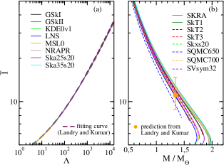
Figure 7: $\bar{I}$ as a function of (a) $\Lambda$, and (b) $M/M_{\odot}$. The same parametrizations are used in both panels. Dashed orange curve: fitting curve of Ref. phil18 . Orange circle: predictions from Ref. phil18 for the dimensionless moment of inertia of the PSR J0737-3039 primary component pulsar.

In Ref. phil18 , it was also obtained the range of $\bar{I}_{\star}\equiv\bar{I}(M_{\star})=11.10^{+3.64}_{-2.28}$ for the PSR J0737-3039 primary component pulsar with mass $M_{\star}=1.338M_{\odot}$. Such numbers were determined through the relation between $\Lambda_{\star}\equiv\Lambda(M_{\star})$ and $\Lambda_{1.4}$, known as the binary-Love relation. The combination between the $I$-Love and the binary-Love relations, along with the GW170817 constraint of $\Lambda_{1.4}=190^{+390}_{-120}$ coming from the LIGO and Virgo Collaboration, allowed the authors to establish the limits given by $\bar{I}_{\star}=11.10^{+3.64}_{-2.28}$. As one can see in Fig. 7b, the CSkP present $9.62\leqslant\bar{I}_{\star}\leqslant 13.01$, values which lie inside the predicted range.

IV Summary and Conclusions

In this paper we have revisited the Skyrme parametrizations that were shown to satisfy several nuclear matter constraints in Ref. dutra12 , named as the consistent Skyrme parametrizations (CSkP), and confronted them with astrophysical constraints and predictions on the GW170817 event studied by LIGO and Virgo Collaboration in recent papers ligo17 ; ligo18 . Concerning the applicability of these nonrelativistic models at the high density regime of the stellar matter, we have shown that causality is not broken at the energy density range of interest, as one can see from Fig. 2, and from the comparison with the central energy density obtained from the CSkP and presented in Table 1. Our calculations also pointed out to a radius range of $\mbox{10.36~{}km}\leqslant R_{1.4}\leqslant\mbox{12.55~{}km}$ according to the predictions of the CSkP. It was also shown that only the GSkI, KDE0v1, MSL0, NRAPR, and Ska35s20 parametrizations are able to produce neutron stars with mass around $2M_{\odot}$, value established form observational analysis of PSR J1614-2230 nature467-2010 and PSR J0348+0432 science340-2013 pulsars. They also establish the more stringent range of $11.86~{}\mbox{km}\leqslant R_{1.4}\leqslant 12.55~{}\mbox{km}$ for the canonical star radius. This range is similar to the one found in Ref. tsang19 , namely, $11~{}\mbox{km}\leqslant R_{1.4}\leqslant 12~{}\mbox{km}$, in which the authors analyzed 5 out of more than two hundred Skyrme parametrizations also investigated in the work. In their study, they also used a piecewise way to construct the EOS, namely, the BPS equation for the outer crust, the same form of the polytropic equation of state as in the present work ($P=A+B\mathcal{E}^{4/3}$), the Skyrme model for the core, and finally, another polytropic form ($P\sim\rho^{\gamma}$) for the density region above $3\rho_{0}$.

Concerning the predictions of the CSkP on the recent GW170817 event, it was shown that all CSkP, except the SQMC650 one, present a mass-radius profile in full agreement with the constraint region given in Ref. ligo18 . Furthermore, by investigating the results regarding the canonical star ($M=1.4M_{\odot}$), our results pointed out to a correlation given by $\Lambda_{1.4}\approx 3.16\times 10^{-6}R_{1.4}^{7.35}$ between the dimensionless tidal deformability and the radius. From this correlation, we found that the CSkP present values of $\Lambda_{1.4}$ completely inside the ranges of $\Lambda_{1.4}\leqslant 800$ ligo17 and even the recent one given by $\Lambda_{1.4}=190_{-120}^{+390}$ ligo18 , as one can see in Figs. 4 and 5. We have also calculated the dimensionless tidal deformabilities of the binary neutron stars system, $\Lambda_{1}$ and $\Lambda_{2}$ (see Fig. 6), and found that the CSkP are completely inside the region defined by 90% credible region in the $\Lambda_{1}\times\Lambda_{2}$ graph, predicted by the recent paper from LIGO and Virgo Collaboration ligo18 . In addition, we verified that the prediction presented in Ref. phil18 on the dimensionless moment of inertia for the PSR J0737-3039 pulsar, namely, $\bar{I}_{\star}=11.10^{+3.64}_{-2.28}$, is attained by the CSkP.

As a last comment, we mention that our study refers only to the predictions of the CSkP with their equations of state given in Eqs. (1)-(6), i. e., no hyperons and no hadron-quark phase transitions are considered. Specifically for the first treatment, the interactions between hyperons and nucleons and between hyperons themselves, which are unknown at present, can be modeled in different ways, see for instance, Refs. dutra16 ; sk5 . For the latter, there is not a unique model that effectively mimics QCD, which makes this study also model dependent from the quark matter considerations. A more detailed and complete study of how these treatments can affect the deformability calculations will be addressed in future works.

References

- (1) J. M. Lattimer and M. Prakash, Science 304, 536 (2004).
- (2) F. Ozel, Nature 441, 1115 (2006).
- (3) M. B. Tsang, J. R. Stone, F. Camera, P. Danielewicz, S. Gandolfi, K. Hebeler, C. J. Horowitz, Jenny Lee, W. G. Lynch, Z. Kohley, R. Lemmon, P. Möller, T. Murakami, S. Riordan, X. Roca-Maza, F. Sammarruca, A. W. Steiner, I. Vidaña, and S. J. Yennello, Phys. Rev. C. 86, 015803 (2012).
- (4) M. Baldo and G. F. Burgio, Prog. Part. Nucl. Phys 91, 203 (2016).
- (5) J. M. Lattimer and M. Prakash, Phys. Rep. 621, 127 (2016).
- (6) M. Oertel, M. Hempel, T. Klahn and S. Typel, Rev. Mod. Phys. 89, 015007 (2017).
- (7) R. C. Tolman, Phys. Rev. 55, 364 (1939).
- (8) J. R. Oppenheimer and G. M. Volkoff, Phys. Rev. 55, 374 (1939).
- (9) Tanja Hinderer, Benjamin D. Lackey, Ryan N. Lang and Jocelyn S. Read, Phys. Rev. D 81, 123016 (2010).
- (10) Philipe Landry and Bharat Kumar, Astrophys. J. Lett. 868 L22 (2018).
- (11) K. Yagi, and N. Yunes, Science 341, 365 (2013).
- (12) James M. Lattimer and Madappa Prakash, Phys. Rep. 442, 109 (2007).
- (13) Jocelyn S. Read, Benjamin D. Lackey, Benjamin J. Owen, and John L. Friedman, Phys. Rev. D 79, 124032 (2009).
- (14) B. P. Abbott et al. (The LIGO Scientific Collaboration and the Virgo Collaboration), Phys. Rev. Lett. 119, 161101, (2017).
- (15) B. P. Abbott et al. (The LIGO Scientific Collaboration and the Virgo Collaboration), Phys. Rev. Lett. 121, 161101 (2018).
- (16) J. Aasi et al. (LIGO Scientific Collaboration), Class. Quant. Grav. 32, 074001 (2015).
- (17) F. Acernese et al. (Virgo Collaboration), Class. Quant. Grav. 32, 024001 (2015).
- (18) B. P. Abbott et al., Astrophys. J. 848 L13 (2017).
- (19) A. Goldstein et al., Astrophys. J. 848 L14 (2017).
- (20) B. P. Abbott et al., Astrophys. J. 848 L12 (2017).
- (21) D. A. Coulter et al., Science 358, 1556 (2017).
- (22) E. Troja et al., Nature 551, 71 (2017).
- (23) D. Haggard et al., Astrophys. J. Lett. 848 L25 (2017).
- (24) G. Hallinan et al., Science 358, 1579 (2017).
- (25) Bharat Kumar, S. K. Biswal and S. K. Patra, Phys. Rev. C. 95, 015801 (2017).
- (26) T. Hinderer, Astrophys. J. 677, 1216 (2008).
- (27) Thibault Damour and Alessandro Nagar, Phys. Rev. D 80, 084035 (2009).
- (28) Taylor Binnington and Eric Poisson, Phys. Rev. D 80, 084018 (2009).
- (29) T. H. R. Skyrme, Proc. Roy. Sco. Lond. A 260, 127 (1961).
- (30) D. Vautherin and D. M. Brink, Phys. Rev. C 5, 626 (1972).
- (31) M. Bender, P. H. Heenen and P. G. Reinhard, Rev. Mod. Phys. 75, 121 (2003).
- (32) J. R. Stone and P. G. Reinhard Prog. Part. Nucl. Phys. 58, 587 (2007).
- (33) M. Dutra, O. Lourenço, J. S. Sá Martins, A. Delfino, J. R. Stone, and P. D. Stevenson, Phys. Rev. C 85, 035201 (2012).
- (34) B. K. Agrawal, S. K. Dhiman, and R. Kumar, Phys. Rev. C 73, 034319 (2006).
- (35) B. K. Agrawal, S. Shlomo, and V. K. Au, Phys. Rev. C 72, 014310 (2005).
- (36) L. G. Cao, U. Lombardo, C. W. Shen, and N. V. Giai, Phys. Rev. C 73, 014313 (2006).
- (37) L. W. Chen, C. M. Ko, B.-A. Li, and J. Xu, Phys. Rev. C 82, 024321 (2010).
- (38) A. W. Steiner, M. Prakash, J. M. Lattimer, P. J. Ellis, Phys. Rep. 411, 325 (2005).
- (39) B. A. Brown, private communication.
- (40) M. Rashdan, Mod. Phys. Lett. A 15, 1287 (2000).
- (41) B. A. Brown, G. Shen, G. C. Hillhouse, J. Meng, and A. Trzcińska, Phys. Rev. C 76, 034305 (2007).
- (42) P. A. M. Guichon, H. H. Matevosyan, N. Sandulescu, and A. W. Thomas, Nucl. Phys. A 772, 1 (2006).
- (43) F. Tondeur, M. Brack, M. Farine, and J. M. Pearson, Nucl. Phys. A 420, 297 (1984).
- (44) J. R. Stone, J. C. Miller, R. Koncewicz, P. D. Stevenson, and M. R. Strayer, Phys. Rev. C 68, 034324 (2003).
- (45) P. Klüpfel, P. -G. Reinhard, T. J. Bürvenich, and J. A. Maruhn, Phys. Rev. C 79, 034310 (2009).
- (46) B. M. Santos, M. Dutra, O. Lourenço, and A. Delfino, Phys. Rev. C 90, 035203 (2014).
- (47) M. Dutra, O. Lourenço, S. S. Avancini, B. V. Carlson, A. Delfino, D. P. Menezes, C. Providência, S. Typel, and J. R. Stone, Phys. Rev. C 90, 055203 (2014).
- (48) Odilon Lourenço, Mariana Dutra, César H. Lenzi, César V. Flores, and Débora P. Menezes, Phys. Rev. C 99, 045202 (2019).
- (49) Tuhin Malik, N. Alam, M. Fortin, C. Providência, B. K. Agrawal, T. K. Jha, Bharat Kumar, and S. K. Patra Phys. Rev. C. 98, 035804 (2018).
- (50) F. J. Fattoyev, J. Piekarewicz and C. J. Horowitz, Phys. Rev. Lett. 120, 172702 (2018).
- (51) N. K. Glendenning, Compact Stars, 2nd ed. (Springer, New York, 2000).
- (52) G. Baym, C. Pethick, and P. Sutherland, Astrophys. J. 170, 299 (1971).
- (53) J. Piekarewicz, and F. J. Fattoyev, Phys. Rev. C 99, 045802 (2019).
- (54) T. Malik, B. K. Agrawal, J. N. De, S. K. Samaddar, C. Providência, C. Mondal, and T. K. Jha, Phys. Rev. C 99, 052801(R) (2019)
- (55) J. Carriere, C. Horowitz, and J. Piekarewicz, Astrophys. J. 593, 463 (2003).
- (56) C. Gonzalez-Boquera, M. Centelles, X. Viñas, and L. M. Robledo, Phys. Lett. B 779, 195 (2018).
- (57) C. Gonzalez-Boquera, M. Centelles, X. Viñas, and A. Rios, Phys. Rev. C 96, 065806 (2017).
- (58) J. Xu, L.-W. Chen, B.-A. Li, and H.-R. Ma, Astrophys. J. 697, 1549 (2009).
- (59) C. Gonzalez-Boquera, M. Centelles, X. Viñas, T. R. Routray, arXiv:1904.06566 (2019).
- (60) S. S. Avancini, L. Brito, Ph. Chomaz, D. P. Menezes, and C. Providência, Phys. Rev. C 74, 024317 (2006).
- (61) J. B. Hartle, Astrophys. J. 150, 1005 (1967).
- (62) K. Yagi, and N. Yunes, Phys. Rev. D 88, 023009 (2013).
- (63) M. Dutra, O. Lourenço, and D. P. Menezes, Phys. Rev. C 93, 025806 (2016); 94, 049901(E) (2016).
- (64) Young-Min Kim, Yeunhwan Lim, Kyujin Kwak, Chang Ho Hyun, and Chang-Hwan Le, Phys. Rev. C 98, 065805 (2018).
- (65) N. Chamel, A. F. Fantina, J. M. Pearson, S. Goriely, Phys. Rev. C 84, 062802(R) (2011).
- (66) S. Goriely, N. Chamel, and J. M. Pearson, Phys. Rev. C 82, 035804 (2010).
- (67) A. F. Fantina, N. Chamel, J. M. Pearson, S. Goriely, Astron. Astrophys. 559, A128 (2013).
- (68) L. Mornas, Eur. Phys. J A 24, 293 (2005).
- (69) Jérôme Margueron, Rudiney Hoffmann Casali, and Francesca Gulminelli, Phys. Rev. C 97, 025805 (2018); 025806 (2018).
- (70) B. Behera, T. R. Routray and S. K. Tripathy, J. Phys. G: Nucl. Part. Phys. 36, 125105 (2009).
- (71) B. Behera, X. Vinas, M. Bhuyan, T. R. Routray, B. K. Sharma, S. K. Patra, J. Phys. G: Nucl. Part. Phys. 40, 095105 (2013).
- (72) P.G. Krastev and B.-A. Li, J. Phys. G 46, 074001 (2019).
- (73) P. B. Demorest, T. Pennucci, S. M. Ransom, M. S. E. Roberts, and J. W. T. Hessels, Nature 467, 1081 (2010).
- (74) J. Antoniadis, P. C. C. Freire, N. Wex et al., Science 340, 448 (2013).
- (75) J. Nättilä, A. W. Steiner, J. J. E. Kajava, V. F. Suleimanov, and J. Poutanen, Astron. Astrophys. 591, A25 (2016).
- (76) A. W. Steiner, J. M. Lattimer, and E. F. Brown, Astrophys. J. 722, 33 (2010).
- (77) H. T. Cromartie, et. al., Nature Astron. Lett. (2019); arXiv:1904.06759.
- (78) Yeunhwan Lim, and Jeremy W. Holt, Phys. Rev. Lett. 121, 062701 (2018).
- (79) Elias R. Most, Lukas R. Weih, Luciano Rezzolla, and Jürgen Schaffner-Bielich, Phys. Rev. Lett. 120, 261103 (2018).
- (80) Nai-Bo Zhang, and Bao-An Li, J. Phys. G: Nucl. Part. Phys 46, 014002 (2019).
- (81) Carolyn A. Raithel, Feryal Ozel, and Dimitrios Psaltis, Astrophys. J. Lett. 857 L23 (2018).
- (82) I. Tews, J. Margueron and S. Reddy, Phys. Rev. C 98, 045804 (2018).
- (83) M. B. Tsang, C. Y. Tsang, P. Danielewicz, W. G. Lynch, and F. J. Fattoyev, arXiv:1811.04888.
- (84) E. Annala, T. Gorda, A. Kurkela and A. Vuorinen, Phys. Rev. Lett. 120, 172703 (2018).
- (85) O. Lourenço, M. Dutra, C. H. Lenzi, M. Bhuyan, S. K. Biswal, and B. M. Santos, Astrophys. J. 882, 67 (2019).
- (86) B. P. Abbott et al. (The LIGO Scientific Collaboration and the Virgo Collaboration), Phys. Rev. X 9, 011001 (2019).
- (87) S. S. Avancini, L. Brito, J. R. Marinelli, D. P. Menezes, M. M. W. de Moraes, C. Providência, and A. M. Santos, Phys. Rev. C 79, 035804 (2009).
- (88) O. Lourenço, C. H. Lenzi, M. Dutra, T. Frederico, M. Bhuyan, R. Negreiros, C. V. Flores, G. Grams, and D. P. Menezes, arXiv:1905.07308.
- (89) C. Y. Tsang, M. B. Tsang, P. Danielewicz, F. J. Fattoyev, W. G. Lynch, Phys. Lett. B 796, 1 (2019).