AutoRegressive Planet Search: Methodology

Abstract

The detection of periodic signals from transiting exoplanets is often impeded by extraneous aperiodic photometric variability, either intrinsic to the star or arising from the measurement process. Frequently, these variations are autocorrelated wherein later flux values are correlated with previous ones. In this work, we present the methodology of the Autoregessive Planet Search (ARPS) project which uses Autoregressive Integrated Moving Average (ARIMA) and related statistical models that treat a wide variety of stochastic processes, as well as nonstationarity, to improve detection of new planetary transits. Providing a time series is evenly spaced or can be placed on an evenly spaced grid with missing values, these low-dimensional parametric models can prove very effective. We introduce a planet-search algorithm to detect periodic transits in the residuals after the application of ARIMA models. Our matched-filter algorithm, the Transit Comb Filter (TCF), is closely related to the traditional Box-fitting Least Squares and provides an analogous periodogram. Finally, if a previously identified or simulated sample of planets is available, selected scalar features from different stages of the analysis – the original light curves, ARIMA fits, TCF periodograms, and folded light curves – can be collectively used with a multivariate classifier to identify promising candidates while efficiently rejecting false alarms. We use Random Forests for this task, in conjunction with Receiver Operating Characteristic (ROC) curves, to define discovery criteria for new, high fidelity planetary candidates. The ARPS methodology can be applied to both evenly spaced satellite light curves and densely cadenced ground-based photometric surveys.

1 Introduction

Searching for transits in stellar light curves has been a very successful approach to discovering exoplanets, yielding several thousand candidates to date. NASA’s Kepler Mission has identified a significant fraction of known exoplanets with densely cadenced, high-precision photometry over nearly 4 years (Borucki et al. 2010). One of the main challenges facing Kepler and other spaced-based planet discovery surveys is the noise and variability of stars with amplitudes comparable to or exceeding the depth of planetary transits (Gilliland et al. 2011). Aperiodic ‘red noise’ is particularly prevalent and challenging to treat (Pont et al. 2006; Carter & Winn 2009; Cubillos et al. 2017). Ground-based surveys suffer a similar problem but with extraneous variability arising predominantly from instrumental and atmospheric conditions. Further discoveries will greatly benefit from statistical methods capable of recovering fainter planetary signals, such as Earth analogues, in systems with high variability.

The problem of identifying transiting planets from photometric time series can be viewed in three stages: (1) a time-domain regression, transform, or interpolation procedure to identify and remove stellar variability; (2) a frequency-domain procedure to construct periodograms in order to find orbital behaviors in the residual time series; and (3) a way to discriminate planetary transit candidates from statistical false alarms and astronomical false positives, such as a decision tree based on various signal statistics.

For the first stage, most researchers use nonparametric approaches including wavelet analysis (Jenkins 2002; Carter & Winn 2009), Fourier filtering (Carpano et al. 2003; Huang et al. 2013), local linear modeling (Roberts et al. 2013), Gaussian Processes regression (Gibson 2014; Aigrain et al. 2016; Luger et al. 2016), Independent Components Analysis (Waldmann et al. 2013), and Singular Spectrum Analysis (Boufleur et al. 2018). The Kepler Team provides PyKE, a detrending procedure based on iterative local polynomial fitting (Vinícius et al. 2017). Here, nonparametric refers to models where no functional relationship is globally applied to the time series, although semi-parametric regressions may be used locally (Ruppert et al. 2003; Takezawa 2005).

For the second stage, the most widely used tool is the Box-fitting Least Squares (BLS) algorithm of Kovács et al. (2002) that acts as a matched filter for box-shaped planetary transits. Other procedures for periodicity searches include periodograms from phase dispersion minimization (Plavchan et al. 2008), Fourier (Sanchis-Ojeda et al. 2014) and Lomb-Scargle (LS; e.g., Hartman et al. 2008) transforms. See Graham et al. (2013b) for a comparison of period-finding methods.

The third stage to distinguish candidate transits from other related periodic behaviors is typically based on the presence of strong peaks in the periodogram and a variety of additional quantitative and qualitative considerations falling under the rubric of ‘vetting’. Automated vetting of planetary transits can utilize procedures such as decision trees and Random Forests (McCauliff et al. 2015; Mislis et al. 2016; Armstrong et al. 2018); these are well-established techniques from modern machine learning methodology (Breiman 2001).

While stellar variability can arise from eclipses, pulsations, and other phenomena, it is most commonly due to magnetic activity including photospheric starspots, chromospheric plages, and reconnection flares (Schrijver & Zwaan 2000). A particular property of solar and stellar activity is autoregressive behavior, wherein future photometric values depend on current and past values. For example, solar flare occurrences are often modeled as ‘avalanche’ processes that produce a $1/f$-type behavior responsible for power law statistical distributions in solar activity properties (Lu & Hamilton 1991; Aschwanden et al. 2016). The frequency distribution of solar and stellar flares is a power law over 10 orders of magnitude in energy. We will see below that $1/f$-type ‘long memory’ processes can be treated by certain autoregressive models (Palma 2007).

The autocorrelated characteristics of stellar photometric ‘noise’ leads naturally to the idea that stochastic autoregressive statistical models could be applied to reduce their influence and help reveal faint periodic planetary transits. The simple case of an autoregressive moving average is labeled an ‘ARMA’ model. ARMA-type statistical models were popularized by Box & Jenkins (1970, the latest edition is Box et al. 2015) and are now very widely used in signal processing, voice recognition, and econometrics, among many other applications. These are parametric models where the coefficients quantify the dependency of current values on past ones assuming stationarity (where the behavior is unchanged throughout the time series). While simple ARMA models treat only ‘short-memory’ autocorrelated processes and white noise in stationary time series, more elaborate models allow for non-stationarity and ‘long-memory’ $1/f$-type processes.

As ARMA-type models are low-dimensional global parametric regression models—rather than nonparametric or high-dimensional semi-parametric models —powerful likelihood-based statistical regression procedures can be utilized. The common procedure is to compute maximum likelihood best-fit models, and then choose the most parsimonious one consistent with the data using penalized likelihood measures such as the Akaike Information Criterion (Hamilton 1994; Chatfield 2004). Quantitative automated measures can be used, leaving these procedures with no arbitrary free parameters or subjective choices. In contrast, nonparametric procedures are subject to choices: the smoothing kernel function and bandwidth in Gaussian Processes regression; the basis function, denoising threshold, and band selection in wavelet analysis; and so forth. Well-established statistical goodness-of-fit tests are available to test whether the best model does indeed fit the data well.

Here we develop a three-stage AutoRegressive Planet Search (ARPS) procedure in detail. We start with maximum likelihood fits of integrated (ARIMA) and fractionally integrated (ARFIMA) extensions to the ARMA model, reducing unwanted photometric variability. This is described in §2. Simple ARMA models have been discussed elsewhere for limited aspects of photometric planet searches (Carter & Winn 2009; Wang et al. 2016) and for filling gaps in irregular light curves (Fahlman & Ulrych 1982; Pascual-Granado et al. 2015). The richer ARIMA and ARFIMA families are largely absent from astronomical studies though have considerable potential (Feigelson et al. 2018).

However, the temporal nature of the transits are transformed by the modeling from a periodic box-like transit shape to a periodic double-spike-like shape. This required development of a customized matched filtering algorithm, called here the ‘Transit Comb Filter’ (TCF), to construct periodograms as presented in §3.

In the final stage, ‘features’ from the light curve, ARIMA-type fits, TCF periodograms, and other aspects of the analysis are fed into a machine learning classifier to recover known, and discover new, candidate planet transit systems (§4). The Random Forests extension of multivariate decision tree classification is an effective method for this stage. Receiver Operating Characteristic (ROC) curves help select thresholds for discrimination of promising planet candidates from false alarm and false positive signals.

ARPS methodology thus differs from common planet finding procedures in the following ways: we use principally ARIMA (instead of moving medians, wavelets, or Gaussian Processes regression) to model the star; the TCF periodogram (instead of BLS or LS periodogram) to extract the periodic signals from transits; and (similar to McCauliff et al. 2015) multivariate classification using Random Forests (instead of a univariate measure like periodogram power). Various methodological issues are discussed in §5 with conclusions in §6.

The present study describes the mathematics and analysis procedure underlying the ARPS project, giving examples from observed Kepler light curves. A first companion paper (Caceres et al. 2019) will apply the method to the full sample of $\sim 200,000$ stellar light curves from NASA’s Kepler mission. Using the final data release DR-25, these light curves span $\sim$70,000 evenly spaced time stamps with $\sim 15-20\%$ of the time stamps have missing data due to instrumental causes. A second companion paper (Stuhr et al. 2019) investigates through simulation the applicability of ARPS to irregularly spaced ground-based transit surveys. Further studies are in progress applying the methods to data from the space-based TESS mission and ground-based HATSouth survey.

Throughout this paper, we will return to the two Kepler stellar light curves shown in Figure 1 to illustrate the various stages of analysis on realistic astrophysical light curves. The first star has only low-level variability, hardly discernible above the white noise of the instrument. The second star has high amplitude variability far larger than the noise. The notation ‘IQR’ stands for interquartile range, a robust nonparametric measure of spread analogous to the standard deviation for Gaussian distributions.

2 Autoregressive Modeling

2.1 Overview

When a dynamic system varies over time, it is common that its current state depend on its past behavior, in which case the process is said to be autocorrelated. The evolution of such a system need not follow a deterministic path. As might seem natural, time series of many physical processes display stochastic autocorrelated properties. This is often the case with variations in stellar photometry, and thus the key motivation for our approach since a great variety of parametric models have been developed to model these aperiodic, stochastic, temporal behaviors. These models weight the influence of past measured values, not (only) current values as in more common regression situations.

The textbooks of Box et al. (2015), Chatfield (2004), and Shumway & Stoffer (2006), are useful general references and provide further details on the topics introduced throughout this section. Mathematically advanced treatments of ARIMA and ARFIMA models appear in volumes by Hamilton (1994), Palma (2007) and Beran et al. (2013). Additionally, Scargle (1981) and Koen & Lombard (1993) give valuable reviews of these topics oriented towards astronomers.

The utility and power of statistical models and theorems rests on the validity of the underlying assumptions for a given problem. Many statistical inferential procedures, such as ordinary least squares, assume independent and identically distributed (i.i.d.) random variables. But, where autocorrelation is present, independence is absent. Care must be taken with conclusions derived from analyzing dependent data. It has long been known that correlated errors have an impact on statistical modeling, and the effects have been extensively studied (see Anderson 1954, for a review of early work). For example, Cochrane & Orcutt (1949) showed that when the errors are serially correlated, the least-squares estimates are no longer guaranteed to have minimum-variance—though they may still remain unbiased. Furthermore, the usual estimates of variance (and thus standard errors) do not apply, and the use of t and F distributions for confidence calculations are no longer valid (Durbin & Watson 1950). Romano & Thombs (1996) also discuss problems that arise with inference of autocorrelation and ARMA coefficients when the underlying assumptions are not strictly satisfied.

We will avoid spending significant effort addressing these mathematical issues by approaching the models from a more phenomenological point of view. The goal here is to reduce the presence of autocorrelation in order to discover new candidate transiting planets, but there is no need or expectation to calculate the “true” ARMA coefficients underlying the physical phenomena, nor even make the assumption it is the intrinsically “correct” model.

The principal focus of this work are Autoregressive (Fractionally) Integrated Moving Average models, known as ARIMA and ARFIMA. In broad terms, AR(F)IMA models represent a regression of the data as a function of its past state. The AR and MA components reflect the dependence of current values on recently past values, fractional integration reflects long timescale dependencies such as $1/f^{\alpha}$ noise, while integer values reflect drifts in the mean. In the parlance of time series analysis, these three components treat short-memory processes, long-memory processes, and nonstationarity, respectively. These approaches have seen widespread, successful use in other fields ranging from engineering to econometrics. The iterative approach to analyze and apply these models was popularized by the seminal work of Box & Jenkins.

Following standard presentations in time series analysis, we assume that the data are acquired at evenly spaced intervals, although missing data at some time slots is permitted. Discrete measurements of the temporal process $X(t)$ produce a sequence of observations $x_{t}$ where $t=1,2,\ldots,n$. The Kepler long-cadence photometric data are acquired in evenly space 29.4 minute intervals, but many other astronomical datasets are unevenly spaced.

Though not as pervasive as in other fields, simple ARMA-type models are increasingly used in time domain astronomy, currently around 25 studies annually (Feigelson et al. 2018). The richer classes of ARIMA and ARFIMA models that treat non-stationarity and long-memory ‘red’ noise as well as short-memory processes only rarely appear in astronomical studies. ARFIMA is used by Stanislavsky et al. (2009) to characterized solar flaring in the X-ray band. For irregularly spaced data, the model can be reconfigured as a continuous-time process. Simple CAR and CARMA models are used for analysis of quasar light curves (Kelly et al. 2014), but broader CARFIMA models (Tak & Tsai 2017) have yet to be applied. Eyheramendy et al. (2018) develop an important generalization, nicknamed IAR for the Irregular AutoRegressive model, that treats non-Gaussian errors.

We note that autoregressive modeling is most effectively used after systematic variations due to instrumental or atmospheric conditions are reduced. Widely used algorithms for this problem include the Transit Filter Algorithm (Kovács et al. 2005), the SysRem algorithm (Tamuz et al. 2005), and Presearch-Data Conditioning (Stumpe et al. 2012). But ARIMA-type techniques can be used even when systematic effects are not fully removed. The mathematics makes no distinction between autocorrelated variations intrinsic to the star from those arising from the observational process.

2.2 Time Series Diagnostics

Figure 1: Example time series and corresponding (P)ACF for KIC 001724719 (Kepler-1569 with P=5.79 day transit period) and KIC 010024701 (KOI K02002.01 with P=14.4 day). We show here only a few percent of the full Kepler light curve that extends for $\sim 1500$ days. The ordinate shows the median-subtracted stellar flux in electrons per second after application of the Kepler Team Pre-Search Data Conditioning Pipeline module that removes most instrumental effects. IQR gives the Interquartile Range of PDC Flux for the full light curve. The autocorrelation function plots are truncated above 0.5.

The need for autoregressive modeling can be determined by evaluating the presence of correlated noise in the time series under study. The Autocorrelation Function (ACF) is a fundamental nonparametric measure of autocorrelation in stationary time series. It calculates the degree of correlation between a series and time-lagged values of itself over the entire time series. Like the Fourier and wavelet transforms, all information in a time series is maintained in the ACF if an unlimited number of coefficients are kept. The advantage of the ACF is that it concentrates short-memory autocorrelation into a few coefficients, even if it is distributed weakly throughout the time series. The Partial Autocorrelation Function (PACF) is a variant of the ACF that measures the lagged correlation while controlling for the effects contributed by intermediate lags.

The cross-correlation between two time series is defined by

$$\operatorname{corr}(x,y)=\frac{E[(x-\mu_{x})(y-\mu_{y})]}{\sigma_{x}\sigma_{y}}$$ (1)

where $x$ and $y$ are two time series with means $\mu_{i}$ and standard deviations $\sigma_{i}$, and $E$ is the expected value. The ACF at lag $k$ corresponds to the correlation between the random variables $x_{t}$ and $x_{t-k}$, and can thus be written as

$$\operatorname{ACF}(k)=\operatorname{corr}(x_{t},x_{t-k})=\frac{E[(x_{t}-\mu_{x})(x_{t-k}-\mu_{x})]}{\sigma_{x}^{2}}$$ (2)

Note that at lag 0 the ACF always equals 1 since the numerator simply corresponds to the constant variance of the series.

While the ACF gives a measure of the memory of the process, the PACF seeks to identify the direct individual contribution from the $k$-th lag, removing the effects of the other intermediate lags. The PACF for a stationary process is given by

$$\operatorname{PACF}(1) = \operatorname{corr}(x_{1},x_{0})=\operatorname{ACF}(1)$$ (3)

$$\operatorname{PACF}(k) = \operatorname{corr}(x_{t},x_{t-k}|x_{t-1},\dotsc,x_{t-(k-1)})\quad k\geq 2$$

where these coefficients are estimated by fitting autoregressive models of successively higher orders. Examples of ACFs and PACFs appear in Figures 1-3.

In addition to the ACF and PACF, hypothesis tests exist to evaluate whether a sequence of data has correlated noise. The Durbin-Watson test (Durbin & Watson 1950, 1951) measures serial (lag=1) autocorrelation, and the Ljung-Box test (Ljung & Box 1978) is a portmanteau test for all lags; they are commonly applied to the residuals of a regression model. Related tests include: the Anderson-Darling and Jarque-Bera tests for normality; the Breusch-Pagen and White tests for heteroscedasticity; and the Augmented Dickey-Fuller and Kwiatkowski-Phillips-Schmidt-Shin tests for stationarity. These are described in textbooks for econometrics (Enders 2014; Greene 2017; Hyndman & Athanasopoulos 2014). We also make use of the Breusch-Godfrey test (Breusch 1978; Godfrey 1978) which generalizes the Durbin-Watson test for lags $k>1$.

2.3 (Non)Stationarity and the Differencing Operator

Figure 2: Time series and corresponding (P)ACF after differencing operation is applied to the lighturves shown in Figure 1. Note the strong, but not complete, reduction in noise and autocorrelation compared to Figure 1.

A time series is stationary when its properties do not change over time, so that its global characteristics (such as mean, variance, and ACF) are identical irrespective of when it is observed. Specific local values will, of course, vary between different segments of time. More formally, strongly stationary processes have a joint probability distribution that is independent of time. ARMA models require wide-sense (or weak) stationarity, where the first two moments—the mean and autocovariance—remain approximately constant over time and the correlation structure depends only on the lag of the observations.

Stationarity is violated when a trend in the mean is present. But nonstationarity can also be present in stochastic processes when the system does not revert to the mean when subject to random shocks. The physicist’s ‘random walk’ is nonstationary in this sense; mathematically, the time series is said to have a unit root. Trends can be reduced by (local) regression techniques, and unit root nonstationarity can be reduced by applying the differencing operator (below). Strictly periodic variations, however, are a type of nonstationarity that is not effectively treated in this fashion and should be modeled using frequency domain techniques.

Aperiodic cyclic behaviors, often called quasi-periodicities, can still arise from a stationary stochastic process even when there is no physical origin for periodicity such as stellar rotation or planetary orbit. Indeed, ARMA-type processes often produce quasi-periodicities that change or dissipate on long timescales; see Vaughan et al. (2016) for an astronomical perspective. Long-memory $1/f^{\alpha}$ autocorrelated processes can be stationary or nonstationary depending on the value of $\alpha$. Time series where the mean values drift or non-recurring outbursts are also nonstationary. More generally, any deterministic function $X=f(t)$ can cause nonstationarity.

Astronomical time series are often nonstationary. A Mira variable star exhibits long-term nonstationary trends in brightness. A solar-type star can exhibit quasi-periodic variations due to rotationally modulated starspots. The X-ray emission from the accreting stellar black hole binary GRS 1915+105 is a famous example where the source shifts between more than a dozen different modes of variations (Belloni et al. 2000). Astronomers commonly trace these behaviors with a local regression procedure, such as a moving average or Gaussian Processes regression, or with wavelet analysis. But a very simple, and often effective, method for reducing many forms of nonstationarity is through differencing. For the backshift operator $B$ defined as

$$Bx_{t}=x_{t-1}$$ (4)

and the resulting differenced series is given by

$$x^{\prime}_{t}=x_{t}-Bx_{t}=x_{t}-x_{t-1}$$ (5)

This is a transform to address the presence of nonstationarity, much in the same manner as log transforms are used to deal with wide ranges and heteroskedasticity. One can also view the differencing operation as a high-pass filter which removes the long-scale variations while leaving short-term fluctuations. The operator takes the point-to-point difference of the original data (i.e. $x_{t}-x_{t-1}$), to create a new stationary time series. This new series of the changes in the data can then be modeled with the autoregressive methods further described in §2.4.4.

Formally, differencing a series is meant to only address certain types of nonstationarity, like a stochastic trend component. In practice a single application of the differencing operator to a nonstationary time series is often sufficient to render it (approximately) stationary irrespective of the exact nature of the nonstationarity. Differencing can increase noise levels if the original time series is Gaussian white noise, but usually decreases noise when autocorrelation is present.

Figure 2 shows the effects of differencing on the two Kepler light curves shown in Figure 1.

2.4 Modeling Autocorrelated Data

Figure 3: Residual time series and corresponding (P)ACF after autoregressive modeling is applied to the data shown in Figure 2. The residuals show no significant autocorrelation and are close to Gaussian white noise.

The ACF (§2.1) and differencing operators (§2.2) are $nonparametric$ transforms of stationary and nonstationary time series, respectively. The ARPS analysis is centered on $parametric$ modeling of autocorrelated time series, treating both stationary and nonstationary cases.

We consider the large class of ARMA-type models where ARMA is an acronym for ‘autoregressive moving average’. The class is very broad with important variants such as VARMA (‘vector’ ARMA for multivariate time series with lags), CARMA (‘continuous’ time ARMA for interpolating irregularly spaced observations), and SARMA (‘seasonal’ ARMA with a strictly periodic components). There are also models like ARCH and GARCH (‘generalized autoregressive conditional heteroskedasticity’) to treat data with non-constant, autocorrelated variance. The 2003 Nobel Prize in Economic Sciences was awarded to Robert Engle for development of the ARCH model that treats volatility where the noise values are also parametrized as an autoregressive process. In the ARPS analysis, we concentrate on two ARMA variants: Autoregressive Integrated Moving Average (ARIMA) models which can deal with nonstationarity and, and ARFIMA models which also treat long-memory processes by allowing fractional integration.

These models serve to phenomenologically characterize the behavior of an autocorrelated stochastic process, and in some contexts, predict its evolution. In many situations, apparently complicated and stochastic time series are actualizations of relatively simple models that depend on only a few parameters describing the autocorrelated behavior. Of key importance is that these methods are designed to model stochastic processes where the random component of the series has a direct effect on its evolution due to the correlated structure.

2.4.1 Autoregressive (AR) Process:

If the value of a variable at a given point in time is influenced by its past values, the model is said to be autoregressive; sequential observations in this scenario are not independent. To account for this effect, a stationary time series can be modeled as a linear combination of its lagged values plus an additional random noise term. A pure AR process can be seen as simple regression problem, with the current state represented as a linear combination of past values. An AR(p) process is modeled by

$$x_{t}=\phi_{1}x_{t-1}+\phi_{2}x_{t-2}+\ldots+\phi_{p}x_{t-p}+\epsilon_{t}$$ (6)

where $\epsilon_{t}$ is a normally (Gaussian) distributed random error with zero mean and unknown variance, $\epsilon_{t}=N(0,\sigma^{2})$, $p$ is the order of the process (i.e. the number of lags in the model), and $\phi_{i}$ are the corresponding coefficients for each lag up to order $p$. The values of $\phi_{i}$ can thus be calculated, for example, via least squares or maximum likelihood estimation. Additionally, the sum of the parameters are constrained to be less than one for stationary processes. An artificial case where all $\epsilon_{t}$ values are zero can mimic a strictly periodic time series.

AR processes have a close link to the ACF and PACF discussed in §2.2, with each AR model having a characteristic structure. For an example, an AR(1) process can be identified by a exponentially-decaying ACF, with a single spike at the first lag in its PACF. Higher order models exhibit similar decay in their ACF and have a sharp cutoff in their PACF at the lag corresponding to the maximum order of the process.

2.4.2 Moving-Average (MA) Process

When a variable is correlated with previous error terms in the series, the process can be considered a moving-average of random shocks that occurred in the recent past. The errors commonly designated ‘innovations’ in the econometrics and statistics literature. While AR models are influenced by previous values of the series, MA models trace the influence of previous random innovations that perturbed the system. Here the random noise term is intrinsically tied to the evolution of the series, and is not an independent and separate effect; each new random value adds information to the series. An MA(q) model is described by

$$x_{t}=\epsilon_{t}+\theta_{1}\epsilon_{t-1}+\theta_{2}\epsilon_{t-2}+\ldots+\theta_{q}\epsilon_{t-q}$$ (7)

where $\epsilon_{t}$ is the error term for the $t$-th time point, $\theta_{i}$ is the coefficient for each lagged error term up to order $q$.

Similarly to AR processes, MA models can also be identified through their (P)ACF, but with reversed behavior. A MA(1) process has a exponentially-decaying PACF, with a sharp ACF cutoff at the lag corresponding to the maximum order of the process. Fitting MA models is more complicated than fitting an AR model, since here the covariates are a value that is not directly observed—namely $\epsilon_{i}$, the error terms. The parameters are typically calculated through an iterative procedure.

2.4.3 Integrated Process

In the presence of nonstationarity, stationarity can often be approximated through the differencing operation discussed in §2.2. A series is created by taking the point-to-point difference in values, which may then be modeled as a stationary ARMA process. To recreate the original series and undoing the differencing, the series is “integrated” back. The order of an integrated process refers to the number of differences needed to achieve stationarity for a given series. Often, a single difference is sufficient to achieve approximate stationarity.

A pure integrated process (that is, without any ARMA components) can be described by

$$(1-B)^{d}x_{t}=\epsilon_{t}$$ (8)

where $d$ is the order of differencing and $B$ is the backshift operator defined by $Bx_{t}=x_{t-1}$. When $d$ is a positive integer, we referred to it as an integrated process; when $d$ is allowed to take non-integer values, the series is fractionally integrated. Equation (5) corresponds to the special case where $d=1$ in the more general description presented here. When a process is not stationary, significant correlation can be observed in the ACF up to very high lags.

As variable astrophysical processes like magnetic activity in stars or disk accretion in quasars are not restricted to following a deterministic functional form $X(t)=f(t)+\epsilon$ over extended times, we must be prepared to handle stochastic nonstationary behaviors such as random walks. A large class of such behaviors are difference stationary and can thus be readily treated within the ARIMA generalization of the ARMA model.

2.4.4 ARIMA and ARFIMA

The three components described can be incorporated into one equation to jointly model more complex processes. ARIMA models combine equations (6)-(8) into a single regression procedure where the $\theta$ and $\phi$ coefficients are simultaneously inferred for the entire time series, and $d$ is either determined by the user or estimated separately. The ARIMA model can be written as

$$(1-B)^{d}x_{t}=\sum_{i=1}^{p}\phi_{i}x_{t-i}+\sum_{j=1}^{q}\theta_{j}\epsilon_{t-j}+\epsilon_{t}$$ (9)

Generally, the best fit parameters for ARIMA-type models are determined using maximum likelihood estimation. The calculation is made for a range of orders $p$ and $q$, and the optimal model is chosen based on some quantitative measure, such as the Akaike Information Criterion (AIC).

A variant of interest in astrophysics is when $d$ is a fraction rather than an integer; the process is called ‘fractionally integrated’ ARMA, abbreviated ARFIMA or FARIMA (Palma 2007). When $0<d<0.5$, the result is a stationary long-memory autocorrelation with a power law behavior in both the autocorrelation function, $ACF(k)\propto k^{2d-1}$ for lag $k$, and in the Fourier spectral density, $f(\nu)\propto|\nu|^{-2d}$ for frequency $\nu$. The process is nonstationary for $d>0.5$. The ARFIMA parameter $d$ is arithmetically connected to $\alpha$ in the physicists’ $1/f^{\alpha}$ ‘red noise’ component where $\alpha=2d$, and is connected to the econometrician’s Hurst parameter, $H=d+0.5$.

A mathematically profound basis for the effectiveness of ARMA-type models is the Wold Decomposition Theorem, which guarantees that any time series can be decomposed into the deterministic part plus an infinite sum of the innovations (Wold 1938). An ARIMA$(p,d,q)$ model is a parsimonious approximation to this decomposition.

Figure 3 shows how ARIMA-type modeling can reduce autocorrelation and noise in a Kepler light curve that the differencing operator alone (Figure 2) did not remove. We have found that ARIMA and ARFIMA are highly effective in reducing non-planetary stellar variability for a large fraction of Kepler stars (Caceres et al. 2019). This is consistent with the widespread success of ARIMA models for modeling and forecasting a wide range of time series on other fields. ARIMA models are applied to model road accidents, stock prices, wind and weather fluctuations, solar irradiance, and innumerable other stochastic processes in human and physical systems. ARFIMA models are less commonly used, but have been applied to model inflation and other macroeconomics measures, erratic heart beats in cardiology, and a variety of forecasting situations.

3 Transit Comb Filter and Periodogram

3.1 Motivation

After investigating the effectiveness of ARIMA-type modeling to characterize and remove unwanted stellar variability, we now turn to the search for faint planetary transit signals in the model residuals. Transits have the crucial property of strict periodicity, so that spectral models that quantify intensity variations as a function of frequency (or equivalently, period) will concentrate the transit signal. Most transit detection techniques use periodograms produced by quasi-Fourier procedures such as the Lomb-Scargle (Scargle 1982) or matched filters such as the Box-fitting Least Squares (BLS) algorithm (Kovács et al. 2002).

The BLS approach fits a periodic series of box-shaped transits testing a number of different periods, phases, and transit durations. This approach can be equated to using a matched filter, where a signal is processed with a filter of the exact shape expected (although the box is only an approximation of a transit’s shape). For a signal in Gaussian noise, the matched filter is equivalent to the maximum likelihood estimator. Thus we follow suit by designing a new matched filter algorithm to optimize the search for the modified transit signal.

Figure 4: Schematic of box-shaped transits (left) and the effects of differencing (right). A similar effect can occur from autoregressive modeling even without differencing.

Figure 5: Schematic of the Transit Comb Filter.

While the BLS algorithm could be applied to autoregressive residuals, its performance will be degraded due to the differencing operation described in §2.3. While ARIMA models are quite effective at reducing the noise inherent in stellar light curves (§2.4.4), this gain has a cost. Differencing and autoregressive modeling affects the shape of the transit signal both in the case of a toy-model box transit (Figure 4) and for real Kepler stars (Figure 6). The periodic box-shaped dip in a stellar light curve due to a planetary transit is transformed by the differencing operator into a distinctive periodic double-spike pattern. The first spike is a decrease in flux due to the ingress of the planet, and the second spike is an increase in flux due to the egress of the planet. During the intervening duration of the transit, the flux is constant so the differenced time series returns to zero. Additionally, random noise will be superposed on these features.

In order to best search for this modified signal expected in the stellar light curve residuals after ARIMA modeling, we devise a filtering algorithm to match its shape that we call the Transit Comb Filter (TCF), due to its comb-like shape, and use it to create a new periodogram.

Figure 6: light curves of KIC 001724719 (left) and KIC 010024701 (right) folded at the planetary transit period at three stages of ARPS analysis: original light curve (top), after differencing (middle), and residuals from the ARIMA model (bottom).

3.2 Matched Filter and Parameter Estimation

The schematic in Figure 5 shows the parameters of the transit. As shown in the lower panels, the shape of the periodic signal is a periodic sequence of Dirac delta functions denoted $\Shah(t)$, known as a Shah function in electrical engineering and as a Dirac comb in mathematics, convolved with a down-up double spike. We call the resulting sequence a Transit Comb.

Consider the simplified approximation where the evenly-spaced time series observed by Kepler is a combination of a transit component and a white noise component,

$$x_{t}=s_{t}+\epsilon_{t}$$ (10)

where, $x_{t}$ is the data (in ARPS, these are the residuals after ARIMA modeling), $s_{t}$ is the planetary transit signal shown in Figure 5, and $\epsilon\sim N(0,\sigma^{2})$ is homoscedastic white noise with zero-mean and variance $\sigma^{2}$. We assume the residuals are approximately distributed as white noise, since after “whitening” the signal using the ARIMA models presented in §2, most of the autocorrelated behavior should have been removed.

Let the filter $f_{t}$ have a known shape parameterized by period $P$, phase $\phi$, and duration $d$. Factoring out the transit depth $A$, any realization of the signal $s_{t}$ corresponds to a scaled copy of $f$ and is given by

$$s_{t}=A\cdot f_{t}(P,\phi,d)$$ (11)

We can estimate the optimal parameters $(A^{*},P^{*},\phi^{*},d^{*})$ of $s_{t}$ by minimizing the squared residuals between $s_{t}$ and the observed data, $x_{t}$. Thus

$$A^{*},P^{*},\phi^{*},d^{*}=\operatorname*{argmin}_{A,P,\phi,d}\sum_{t}(x_{t}-s_{t})^{2}=\operatorname*{argmin}_{A,P,\phi,d}\sum_{t}(x_{t}-A\cdot f_{t}(P,\phi,d))^{2}.$$ (12)

Expanding the square and separating the summations (omitting the arguments of $f_{t}$ to simplify the notation) gives

$$A^{*},P^{*},\phi^{*},d^{*}=\operatorname*{argmin}_{A,P,\phi,d}\left[\sum_{t}(x_{t})^{2}+A^{2}\sum_{t}f^{2}_{t}-2A\sum x_{t}f_{t}\right]$$ (13)

The first term in (13) corresponds to the observed data and can be ignored in the minimization since it is constant with respect to the transit parameters. Reversing the sign to turn it into a maximization problem and simplifying gives

$$A^{*},P^{*},\phi^{*},d^{*}=\operatorname*{argmax}_{A,P,\phi,d}\left[2A\sum x_{t}f_{t}-A^{2}\sum_{t}f^{2}_{t}\right]$$ (14)

An analytic solution for $A^{*}$ as a function of the remaining parameters can be obtained from (14) by taking its derivative with respect to $A$ and setting it equal to zero, yielding

$$A^{*}(P,\phi,d)=\frac{\sum_{t}x_{t}f_{t}}{\sum_{t}f_{t}^{2}}.$$ (15)

The optimal parameter estimates are are then obtained by maximizing

$$P^{*},\phi^{*},d^{*}=\operatorname*{argmax}_{P,\phi,d}\frac{(\sum_{t}x_{t}f_{t})^{2}}{\sum_{t}f^{2}_{t}}.$$ (16)

We now define the shape of the filter in terms of measurable quantities. For the denominator of equation (16), we first recognize that the number of transits $k$ in a time series has $N$ data points is

$$k=\left\lfloor\frac{N-\phi}{P}\right\rfloor+1$$ (17)

where $\lfloor x\rfloor$ is the largest integer less than or equal to $x$. The filter $f_{t}$ has a value of 1 or $-1$ at the location of each “comb tooth” (parametrized by $P^{*}$, $\phi^{*}$, and $d^{*}$), and equals zero everywhere else. Therefore $f_{t}^{2}=|f_{t}|$ which has a value of 1 at each spike and zero elsewhere. Since there are $k$ transits with two spikes each, then $\sum|f_{t}|=2k$.

The numerator of equation (16) can also be simplified by noting that the product $x_{t}\cdot f_{t}$ equals $-x_{t}$ when $t$ corresponds to a downward spike (ingress), and $x_{t}$ when it corresponds to an upwards spike (egress). The ingress spike occurs at times $t$ that are multiples of the period plus a phase shift, and the egress spikes occurs at the same value plus an additional time shift due to the duration. Therefore the updated equation is

$$P^{*},\phi^{*},d^{*}=\operatorname*{argmax}_{P,\phi,d}\frac{\left(\sum_{i=1}^{k}x_{(i-1)P+\phi+d}-x_{(i-1)P+\phi}\right)^{2}}{2k}$$ (18)

This formulation greatly reduces the number of computations required, since it omits all other values of $t$ that evaluate to zero. The optimal values at which equation (18) is maximized then correspond to the best estimate for the transit parameters.

We now have the ingredients for constructing a periodogram based on this least-squares search for periodic double spikes by taking a sequence of periods and for each maximizing (18) to find $A^{*}$ and $\phi^{*}$. The pseudocode for the TCF implementation is shown in Figure 7. The optimal value of (18) gives a measure of the signal strength or “power” at the given period, and these values over all periods evaluated allows us to create a periodogram. The ‘best’ period $P^{*}$ can reasonably be chosen to give the maximum power in the periodogram, or the maximum signal-to-noise ratio (SNR) with respect to local noise in the periodogram.

The application to the ARIMA residuals of the two Kepler stars is shown in Figure 8. In each case, we see a clear ‘best’ period with factor-of-two harmonics as expected from a true periodicity. Here the same period has maximum power and maximum SNR in the periodogram, but this is not necessarily the case.

Algorithm 1: Transit Comb Filter pseudocode

Equally-spaced light curve, periods (in units of cadence)

Result: TCF periodogram, transit parameters at each period

     Start

         for each period do

              for each phase do

    // Dot product between Shah filter and light curve

    $sum_{phase}\leftarrow\displaystyle\sum^{N}_{i=1}{}_{i}x_{i}$ 

              end for

              for each duration do

    // Average between egress and ingress

    $depth_{phase}\leftarrow\displaystyle\frac{(sum_{phase+duration}-sum_{phase})}{2N}$ 

    $power_{phase}\leftarrow\displaystyle\frac{(sum_{phase+duration}-sum_{phase})^{2}}{2N}$ 

              end forRecord $power$, $depth$, $duration$, and $phase$ corresponding to the maximum

  value of $power_{phase}$, for current $period$ 

         end for

     End

End

Figure 7: Algorithm: Transit Comb Filter pseudocode

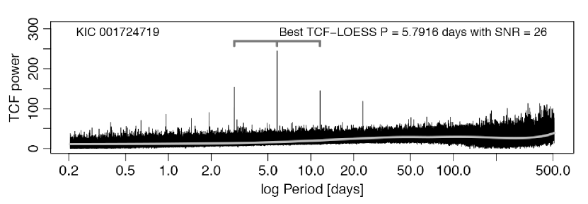
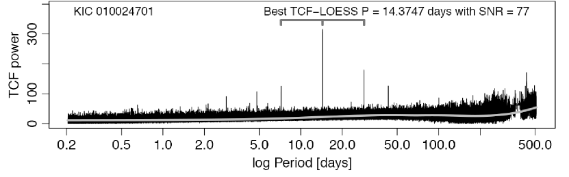
Figure 8: Transit Comb Filter periodograms for ARIMA residuals of the two Kepler stars showing matched filter power for $\sim$500,000 periods ranging from 0.2 to 500 days. The gray curve shows the LOESS smoothed estimator for the median of the TCF power. The periodogram peak is marked with 1/2-times and 2-times harmonics. The signal-to-noise ratio is calculated with respect to noise in a window around the peak.

Careful consideration is needed for the choice of periods to be examined. While it is common practice to sample periods for a periodogram in constant-frequency steps, Ofir (2014) notes that this approach may not be optimal for transit detection when using an algorithm like BLS due to unnecessary oversampling of short periods or damaging undersampling of long periods. We adopt Ofir’s recommendation to use $\Delta f\simeq q/S$ where $q$ is the duty cycle (i.e., transit duration in fractional phase) of the signal and $S$ is the full span of the time series in candences. Since the TCF focuses on the ingress/egress spikes, the duty cycle would be $q\simeq 1/P$ where $P$ is the period, giving a corresponding relation

$$\Delta f\simeq\frac{f}{S}.$$ (19)

We can arrive to a similar conclusion estimating the error of a transit’s ingress time when using an incorrect period. If one assumes that the transit’s ingress and the measurement occur instantly, and if the period is incorrect by $\Delta P$, then each transit is delayed by that amount leading to the n-th transit being off by $\Delta P\times n$. A signal with period $P$ observed over a span of time $S$ has at most $n=S/P$ transits so that $\Delta P\simeq P/S$. Inverting this gives the relation in equation (19). An equivalent formulation is to use periods

$$P_{k}=P_{0}\bigg{(}1+\frac{1}{S}\bigg{)}^{k}$$ (20)

where $P_{0}$ is a chosen minimum period and $k$ is a sequence of integers noting the number of points in the periodogram.

A few approximations are made for equations 19-20. Realistic transits do not align exactly with the instant of the first observation, so the $\sim 1$ cadence bin shift over the span of the time series means that later transits may shift into the next cadence bin. Furthermore, ingresses have a finite duration and the observation is integrated over a period of time, which can also lead to a one-cadence shift. To reduce these effects, the ”teeth” of the Transit Comb Filter can be given widths larger than a single cadence.

3.3 Estimating the significance of TCF periodogram peaks

As with other periodograms, evaluation of the False Alarm Rate of peaks in the TCF periodogram is difficult. Except for unrealistic ideal situations, analytic calculations of periodogram significance levels are unreliable for Lomb-Scargle periodograms of irregularly spaced data (Koen 1990; Vaughan et al. 2016; Vanderplas 2018), and even for Fourier periodograms of regularly spaced data (Percival & Walden 1993).

We have found in practice that the distribution of a TCF periodogram powers in the absence of a periodic signal is highly non-Gaussian and with variable mean. In Kepler periodograms, a nonlinear trend is seen with medians rising as period increases. We remove this trend with a smooth local regression fit to the medians of the TCF periodogram using the well-established LOESS algorithm (Cleveland 1981). A similar behavior is found in Box Least Squares periodograms of Kepler light curves as discussed by Ofir (2014) who also recommends nonparametric detrending of the periodogram. After trends are removed by subtracting the LOESS curve, we record the highest-power peaks in the periodogram and estimate a local signal-to-noise ratio (SNR) within a window of nearby period values. This is illustrated for the two Kepler stars in Figure 8.

However, we can assist with evaluating periodogram peak significance by estimating the marginal likelihood of the transit depth parameter $A$, and thereby estimate its signal-to-noise ratio. Section 3.2 noted that $A$ can be factored out of the filter and simply calculated as a function of the other parameters. This is possible because, given parameters $p$, $\phi$, and $d$, determining $A$ is a simple linear problem; the period, phase, and duration fully describe the location of each “box” and all that remains to calculate is its respective amplitude.

We therefore add an additional step of fitting an ARIMA-type model that includes a simple box-shaped model of the transit corresponding to the best TCF period. The incorporation of covariates in ARMA-type modeling is common in econometrics. Our situation is similar to the econometric problem of modeling retail sales with both stochastic autoregressive characteristics and a deterministic weekly cycle; here the period (7 days) and phase (weekday $vs.$ weekend) is known but the amplitude of the cyclical component is unknown. The statistical model is often called ARIMAX for ARIMA with ‘explanatory’ or ‘exogeneous’ variables, or ‘dynamic regression’ (Hyndman & Athanasopoulos 2014; Box et al. 2015).

This idea is formalized by defining an indicator function, $I(t)$, which equals 1 when in transit (as determined by the given $p$, $\phi$, and $d$) and 0 otherwise. These values are obtained from the ‘best’ period in the TCF periodogram. To regress the observed data on this indicator function, the corresponding coefficient of this linear regression corresponds to the depth of the box. That is

$$x(t)=\beta_{0}+\beta_{1}I(t)+\epsilon_{t}$$ (21)

where $\beta_{0}$ fits the global mean, $\beta_{1}$ is the coefficient of the indicator function, and $\epsilon\sim N(0,\sigma^{2})$ is the error term. The $\beta_{1}$ coefficient is the mean offset while in transit (that is, the transit depth).

This deterministic regression is combined with the stochastic ARMA model by dropping the assumption that the error term of equation (21) is white Gaussian noise, but instead is an autocorrelated ARIMA process. The hierarchical regression model with ARMA errors (temporarily ignoring the differencing operator to simplify the notation) then looks like

$$x(t) =\beta_{0}+\beta_{1}I(t)+\eta_{t}$$ (22)

$$\eta_{t} =\sum_{i=1}^{p}\phi_{i}\eta_{t-i}+\sum_{j=1}^{q}\theta_{i}\epsilon_{t-i}+\epsilon_{t}$$

where $\epsilon_{t}\sim N(0,\sigma^{2})$ is the white Gaussian noise term. We now compute the maximum likelihood values in the model (22), estimate the value and uncertainty of the $\beta_{1}$ parameter from the linear regression model, and compute the depth amplitude signal-to-noise ratio

$$SNR(A)\simeq\hat{\beta_{1}}/\widehat{\sigma_{\beta_{1}}}.$$ (23)

Note that signal-to-noise ratio shown in Figure 8 is different from that of equation (22); the former measures significance of the TCF power before a periodicity has been identified, while the latter measures the significance of the transit depth after a periodicity is assumed to be present.

While this ARIMAX approach may seem to be redundant to the earlier ARIMA approach, we find it can be very valuable in assisting the evaluation of the significance of a TCF periodogram peak. In our application to the Kepler 4-year dataset, the ARIMAX $SNR(A)$ from equation (23) proved to be the most important ‘feature’ in the machine learning classifier for identifying planetary candidates and discriminating them from False Positives like blended eclipsing binary stars.

3.4 Comparison of TCF and BLS periodicity search

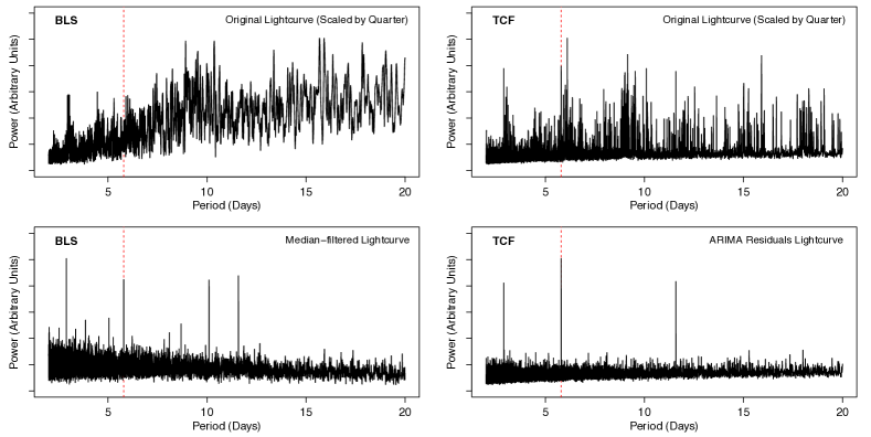
Figure 9: Comparison between BLS (left panels) and TCF (right panels) periodograms for KIC 001724719. The top panels show each algorithm applied directly to the original light curve. The bottom-left panel shows the BLS periodogram of a median-filtered light curve using a 12-hour window. The bottom-right panel shows the TCF periodogram applied to ARIMA residuals. The dashed red line shows the known planetary period.

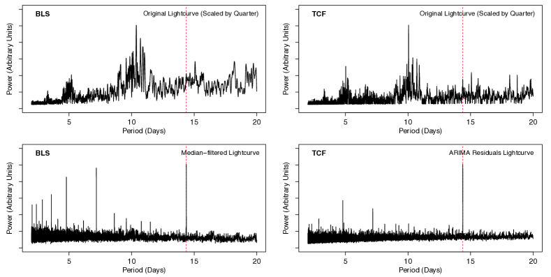
Figure 10: Same as Figure 9 for KIC 010024701.

Figure 8 showed how the TCF algorithm was capable of recovering the transit signal from ARIMA residuals for both of our example stars. To illustrate how this compares with other approaches, we now show a simple application of the BLS algorithm to both stars. These results are summarized in Figures 9 and 10. In each figure, the top panels show BLS and TCF applied to the original PDC light curve (with each quarter scaled to zero-median). The bottom panels show the BLS periodogram applied to a median-filtered light curve with a 12-hour window, and the TCF periodogram applied to the ARIMA residuals. We caution that this comparison of TCF and BLS performance is very incomplete. The mathematical treatments are different, the periodograms measure different quantities, and the sensitivities of the methods may differ when applied to time series with different cadences, stellar noise characteristics, planetary transit depths and durations.

Neither algorithm detects a significant transit signal in the original light curve; this emphasizes the importance of some type of filtering even when a light curve may not exhibit strong variations. After reducing stellar variability, the true planetary periods are clearly seen in both the BLS and TCF periodograms, but the BLS periodogram shows stronger harmonic structure. The harmonic structure can help to confirm the existence of a periodicity, but may also confuse identification of the true peak when the 1/2-times or 2-times harmonics have comparable power. The BLS periodograms also tend to have higher noise at shorter periods than than the corresponding TCF periodograms.

BLS performance will be affected by different filtering procedures such as median filter, Fourier filter, wavelet decomposition, Gaussian Processes or other local regression. There is no mathematical guidance regarding the choice of filter, although properties of the residuals can be compared to improve the choice for a given star. In most of these nonparametric procedures, a suitable bandwidth and/or kernel needs to be selected; the resulting BLS periodogram may be considerably affected by these choices. Most astronomical researchers choose the bandwidth heuristically, while statisticians would recommend bandwidths chosen by cross-validation to minimize the global sum of bias-squared and variance (Wasserman 2007). However, for the purposes of periodic transit detection, the optimal value of this parameter may depend on the exact properties of period, depth, and duration which are unknown for yet-undiscovered objects. The 12-hour boxcar window used for the BLS analysis in Figures 9 and 10 was selected by evaluating the periodogram using different smoothing windows. In practice, this may not be computationally viable when a large range of periods are being tested for many objects.

A serious concern is whether TCF will have reduced sensitivity to transits compared to BLS because the modified Shah function template is matched only to ingress and egress spikes, while the BLS fit includes photometry during the transit as well as the ingress/egress events. The strength of a transit depth in a light curve can be viewed as the product of the depth and $n_{t}$ where $n_{t}$ is the product of the number of transits observed during the observation span and the typical number of points per transit. For a box shape, $n_{t}$ scales with transit duration $d$, while the number of points per transit for TCF is always close to unity (where the exact values depend on the width of the ingress ‘teeth’ chosen for the calculation) independent of duration. We thus expect ARPS analysis to be most sensitive to short-duration transits where TCF inherits the advantages of ARIMA modeling while still retaining most of the transit signal.

The deterioration of TCF sensitivity is linked to period for the simple case of planets in circular orbits with zero inclination. The transit duration is then $d=R_{*}/v_{orb}$ where $v_{orb}=2\pi a/P$ where $R_{*}$ is the stellar radius and $a$ is the planet’s semi-major axis. As Kepler’s Law requires $P^{2}\propto a^{3}$, the transit duration is related to orbital period as $d\propto P^{1/3}$. Therefore, for an algorithm like BLS, the reduction in $n_{t}$ for planets with longer periods is partially offset by the longer duration caused by the slower planetary orbital velocity. Specifically, strength of the BLS periodogram peak will scale as $\sqrt{n_{t}}\propto\sqrt{d/P}\propto P^{-1/3}$. In contrast, the TCF periodogram peak is independent of duration and scales as $\sqrt{n_{t}}\propto\sqrt{1/P}\propto P^{-1/2}$. Comparing a host star with identical planets at orbital periods 1:10:100 days, the BLS periodogram peak weakens as 1.00 : 0.46 : 0.22, while the TCF periodogram peak weakens as 1.00 : 0.32 : 0.10.

We therefore expect TCF to exhibit its best sensitivity with respect to BLS at short periods like $P\simeq 1$ day with moderate deterioration (1 - 0.32 / 0.46 = 30%) at 10 days and stronger deterioration (1 - 0.10/0.22 = 55%) at 100 days. The sensitivity loss does not apply to planets with significant ellipticity and/or inclination where the transit duration can be short even for long period orbits. This calculation also does not evaluate the coefficient in front of these proportionalities; the TCF periodogram peak could be higher or lower signal-to-noise than BLS periodogram peak at any given period for a given planet. We do not know any reliable calculation of the relative sensitivities of the two methods for realistic light curves where complicated treatments (ARIMA modeling, nonparametric wavelet analysis, local regression, or other procedure) have been applied to reduce the aperiodic variability. The possible presence of non-Gaussianity and autocorrelation in the residuals, possible removal of unknown portions of the periodic transit in earlier modeling steps, and complicated alias structure in the periodograms together make it difficult to estimate the signal-to-noise for any periodogram in realistic cases. The cases shown in Figures 9-10 indicate that TCF can perform well in comparison to BLS for these Kepler light curves with periods around $5-15$ days. Its relative performance may be even better for shorter periods including UltraShort Period ($P\leq 1$ day) planets.

4 Classification

4.1 Learning Algorithms & Feature Selection

While a single periodogram can be investigated and assessed by eye, often we have many light curves that need to be evaluated, whether from surveys or simulated data. These large samples provide both a challenge and an opportunity. The large number of objects can make individual assessments prohibitively time consuming and raises the challenge of how to automatically select promising candidates for further exploration while reducing contamination from random statistical variations and from astronomical False Positives such as eclipsing binary light curves. The ability to evaluate the performance of the approach on a wide variety of objects can enable us to make improved statistical statements on the significance of a given discovery. We review the use of learning and classification algorithms to address this issue, and discuss how to define automatic selection criteria for detection. The exact procedure depends on the dataset under study, so our treatment here is schematic.

Quite often, a single attribute such as periodogram power is used to determine whether the signal in a given object is significant enough for scientific interest. Section 3.3 discussed two approaches: estimating the strength of a peak in the periodogram (either its spectral power or its signal-to-noise ratio relative to the local periodogram noise), and assessing the significance of the transit depth within a parametric ARIMAX-type model with both stochastic autoregressive and deterministic periodic components.

But other properties or ‘features’ of the data at different stages of ARPS processing can also assist in evaluate a possible transit. One approach for analyzing time series data is to create summary variables characterizing relevant parts of the data (Wang, Smith & Hyndman 2006). Guiding principles have been developed on the choice of features for multivariate classification (see an overview by Guyon & Elisseeff 2003). Armstrong et al. (2018) gives an example of feature engineering for transit planet detection. Feature selection for classification of ensembles of astronomical light curves outside of exoplanetary detection is discussed by Richards et al. (2011), Graham et al. (2013a), Rimoldini (2014), Benavente et al. (2017), Pashchenko et al. (2018), Cabral et al. (2018), and others. For the ARPS method, we take the approach of incorporating a variety of different measures summarizing both the original light curve as well as intermediate data products from the autoregressive model and the TCF periodogram.

Features that can be used to inform the classifier can include: properties of the star like the magnitude and radius of the star; properties of the original, differenced, and ARIMA residual light curves such as IQR and Durbin-Watson statistic (a scalar measure of the ACF amplitude at lag=1); properties of the TCF periodogram peak such as period, signal-to-noise, and presence of harmonics; and properties of the folded light curve such as shape statistics, depth amplitude and duration, and comparison of even-vs.-odd events.

Hard and soft classification are two common terms used to describe the output from a classification algorithm. The former applies when a specific class prediction is required, while the latter is used when probabilities for each star belonging in each category are calculated instead.

In order to apply supervised learning algorithms we require a “labeled” training set, where the expected output is known. This can take the form of data previously classified through other means, or simulations where the true values are known. For exoplanetary studies, simulations can take the form of injections of artificial transits into real stellar light curves (Christiansen et al. 2016).

4.2 Random Forest

The Random Forest classifier, an extension of classical decision tree classifiers involving sequential splits of the data based on critical values of different variables, is a powerful approach to the selection of new planetary candidates (Breiman 2001). The ’Autovetter’ of the Kepler Team is based on Random Forest decision trees (McCauliff et al. 2015, see also Mislis et al. 2016 and Armstrong et al. 2018). (In contrast, the Kepler Team ’Robovetter’ procedure classifies transits with a thresholded univariate metric based on the shapes of folded light curves, Thompson et al. 2015). Other multivariate machine learning approaches can be considered such as Support Vector Machines and neural networks including Deep Learning convolutional networks.

A Random Forest is an ensemble algorithm made up of a multitude of decision trees (Breiman 2001). Each tree generates many sequential, binary splits of the data based on a single variable in order to discriminate between the categories of the response variable. At each split (called a node), thresholds are tested for predictor variables and the threshold-variable combination which best optimizes a defined criterion is used for the split. Typical criteria for decision tree classification are to decrease Gini impurity or increase information gain.

Random Forests have important advantages over other classifiers for our problem. Since each variable is tested independently and only the relative rank of the values, not their magnitudes, are used for splitting, decision trees – and by extension Random Forests – are not affected by differing units and scales (e.g. logarithmic transformations) of the input variables. Unlike many other machine learning methods, no scale-dependent metric is used. Input variables of potential utility can be proliferated because the method is robust to uninformative variables (Cutler, Cutler & Stevens 2012). Dozens of features can be generated for the method to consider in its optimization of a classifier. Random Forests are computationally fast. Random Forests provide outputs that assist in understanding the basis of the classification: the relative importance of each variable is provided, and any single decision tree can by understood as a sequence of univariate decision rules. In contrast, the output of many other classifiers (such as neural networks) are difficult to interpret.

Decision trees procedures have weaknesses. They are often biased towards variables with greater number of categories, or towards continuous variables instead of categorical ones (Breiman et al. 1984; White & Lio 1994; Loh 2002; Strobl et al. 2007). Measures of variable importance can be biased in such cases (Genuer et al. 2010). Individual trees are often prone to overfitting, and may benefit from additional methods such as pruning (Quinlan 1987). While Random Forests can maintain its predictive power when given highly-correlated predictors (Strobl et al. 2007), it can be overwhelmed if many highly correlated variables lead to similar trees with similar splits (Cutler, Cutler & Stevens 2012). Best performance is achieved when the ensemble’s trees are not strongly correlated.

A ’forest’ is obtained by training an ensemble of trees, each based on a bootstrap resampling of the original data (i.e., a random sample, with replacement, of entries of the data and of the same size as the original data). At each split only a random subset of the predictor variables are used. This allows variables that are slightly less important to still contribute to the decision making, and can also help reduce the bias towards variables with greater number of differing values. Using an ensemble of trees helps overcome some of the weaknesses of individual decision trees, reducing the variance of the global classifier at the expense of additional computational effort and a less intuitive underlying model.

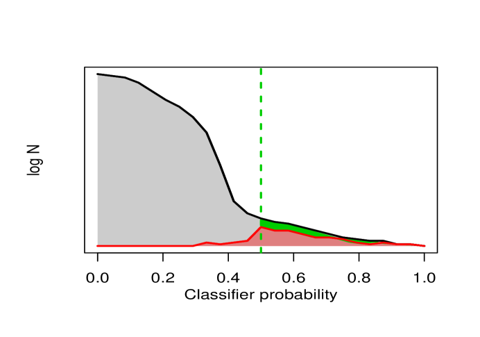
Figure 11: Schematic application of a Random Forest classifier to test data. Dashed green line: subjectively chosen threshold for selection of candidate planets. Red region: Stars with confirmed planets from training set. Green region: Stars with newly discovered candidate planets. Grey region: Unselected stars.

The trees of the forest are combined into a single probabilistic result using bootstrap aggregation, also known as bagging (Breiman 1996a, 2001). Typically, the majority vote of the trees in a Random Forest is used for hard classification, but the vote fractions represent soft classification and provide an estimate of the model’s certainty about its decision. Figure 11 shows a schematic of the class probability estimated by a classifier to discover new candidate planets. Known planetary candidates (red region) make up a small fraction of the full stellar population (grey region) and typically are given a higher score by the classifier. The remaining objects above a certain threshold which are not known candidates (green region) correspond to the discovery space of new candidates. The dashed green line corresponds to the cut-off set to maximize the recovery of known planets while minimizing false positive classifications.

The standard tunable parameters in a Random Forest are the total number of trees to grow and the number of features to test at each split (Cutler, Cutler & Stevens 2012). These two parameters allow generation of a Random Forest: the vote of many trees grown on bootstrap samples of the data (‘bagging’, Brieman 1996b), and random feature selection at each node (‘subspace method’, Ho 1998). It is possible to tweak other parameters, such as tree depth and minimum node splitting size, but this is not commonly done. In standard implementations of Random Forests, trees are fully grown and branches are not pruned to reduce model complexity (Quinlan 1987). In R’s randomForest, the default procedure is to split the data as many times as necessary until each terminal node contains only a single data point. While it may appear unintuitive to grow such complex trees and thus overfit the data, this allows reduction of variance in the ensemble’s prediction through bagging.

The probabilities estimated by this Random Forest model are uncalibrated. Although it has been argued that Random Forest predictions can approximate true posterior probability distributions (Fan et al. 2005), this is a more challenging problem than the simpler case of developing a good discriminator. Furthermore, undersampling the data to address class imbalance during training affects the estimated probability of a model. The modified probabilities do not affect the rank-order of the estimates; this maintains the discriminatory power of the classifier, but affect the probability calibration. Methods do exist to recalibrate the estimates (Dal Pozzolo et al. 2015) and, more generally, to apply classification models to test sets that have different class distributions than the original training set (Elkan 2001; Saerens et al. 2002).

4.3 Training Set Specification

Many textbook cases of classification have unambiguous labels for the desired classes (such as the numbers ‘1’, ‘2’ and ‘3’ in optical character recognition) and no difficulty constructing balanced training sets with similar number of objects in each class (such as ‘cat’ and ‘dog’ in photographs). Both of these issues are problematic in machine learning applications to exoplanet transit detection.

The first problem arises because the ensemble of stellar light curves without known planets is highly heterogeneous, ranging from quiet stars with no noticeable signals, to stars with quasi-periodic rotationally modulated starspots, eclipsing binaries, explosively flaring stars, and other variables. In addition, some light curves may be subject to instrumental and observational effects that mimic some aspects of planetary transits with no relation to the star itself. This wide range of light curve behaviors needs to be properly sampled in the ‘non-planet’ training set to reduce the chance of the algorithm mistaking them for planetary transits.

It is not obvious whether all types of ‘non-planet’ should be grouped into a single class for the Random Forest algorithm, or whether better discrimination will be possible by considering several classes of ‘non-planet’. Care must also be taken for which ‘non-planet’ objects are included since any new transit discoveries must obviously come from systems that previously had no known planets. If a light curve containing a yet-undiscovered planet is used during training with a negative label, then the algorithm could learn that the signal does not originate from a planet and thus fail to discover it. Research groups involved in space-based (McCauliff et al. 2015) and ground-based (Schanche et al. 2018) transit surveys invest great effort in discriminating light curves that are convincingly true exoplanetary surveys from those with some periodic signals that arise from other astronomical causes, such as blended eclipsing binaries. The judgment between ‘certified’ planet candidates and False Positives can be difficult to make.

The second problem is due to the unavoidable geometrical constraint that only a small fraction of planets will have orbital inclinations allowing transits to be detected. This can be compounded by survey sensitivity; for example, a ground-based survey subject to noisy observational conditions may be sensitive only to hot Jupiter transits which are very rare. The result is a highly imbalanced sample; there may be dozens, or even thousands, of stellar light curves without transits for each one with a transit. Furthermore, the small size of the ‘planet’ training set may poorly span the high-dimensional multivariate feature space, give rise to noisy and inaccurate classifiers.

It is possible to down-sample the large class or up-sample the small class to construct artificially balanced training sets for classifier training. The SMOTE algorithm, for example, is widely used for proliferating simulated objects in a small training set (Chawla et al. 2002), and random sampling is used for pruning objects in a large training set. However, it is difficult to overcome extreme class imbalances, as seen in exoplanetary surveys, with these methods.

The Random Forest algorithm has some advantageous properties to address these issues. First, bagging $-$ where many different models vote on their predictions $-$ has been shown to work well even for problems with considerable classification noise due to incorrect class labeled (Dietterich 2000). Random Forest should thus be less susceptible than some other classifiers not only to using stars with unknown disposition as negative labels, but also to mix ups between candidate and false positive status in stars labeled as true transits. Second, the construction of trees with randomized subsamples of the training sets essentially mimics the cross-validation approach to classification without requiring the removal of objects from the sparse ‘planet’ training set. The ‘out-of-bag’ (OOB) predictions of the Random Forest algorithm allow improved estimate of node probabilities and error rates in tree construction. Variants of the Random Forest algorithm can also treat class imbalance (Chen et al. 2004).

4.4 Receiver Operating Characteristic (ROC) Curves

Figure 12: Schematic view of the classification stage for identifying candidate transiting planets. ROC curves for a single parameter measuring the peak in the TCF periodogram (dashed curve), and for a classifier combining the predictive effects of multiple features of the light curve, periodogram and folded light curve (solid curve).

Many approaches, whether univariate or multivariate, perform “soft” classification through a real-valued output such as periodogram power or Random Forests probability. When seeking to predict a specific category (“hard” classification), for example to create a candidate exoplanet catalog or list for follow-up telescopic study, a cutoff threshold must be defined. For the case of discrimination between two classes using a single real-valued feature, ROC curves are a useful tool for both evaluating a classifier’s performance and selecting a threshold value (Hanley & McNeil 1982; Fawcett 2006; Krzanowski & Hand 2009). ROC curves (§4.4) allow us to compare the trade-off between the False Positive Rate (FPR) and the True Positive Rate (TPR) as a function of the cutoff value of some classificatory measure, such as the probability emerging from a Random Forest classifier or the SNR of the peak values in a periodogram. The TPR is the ratio of true positives recovered by the classifier to all events which are actually positive, and similarly, the FPR is the ratio of recovered false positive to all events are in truth negative.

One important use of ROC curves is to compare the classificatory effectiveness of different classifiers (e.g., using different methods, variables, or training sets). The scalar measure called Area Under the Curve (AUC) is often used in this capacity (Bradley 1997). The AUC can be interpreted as the probability that a randomly chosen positive case is ranked higher by the algorithm than a randomly chosen negative case.

For illustration purposes, Figure 12 shows an example ROC curve which could be used to compare two different classification procedures from a classifier of transit $vs.$ non-transit light curves. The ideal location is the top-left corner of the plot, where $TPR=1$ and $FPR=0$. Using known candidates, we can calibrate the metric of interest to a desired combination of TPR and FPR. Several scalar metrics that combine TPR, FPR and related quantities are used including: sensitivity, specificity, precision, false discovery rate, F1 score and Matthews correlation coefficient. This last quantity is designed to be less sensitive to imbalances in training set sample sizes.

5 Discussion

The AutoRegressive Planet Search (ARPS) statistical procedure has three main stages: ARIMA-type modeling of the light curve; TCF periodogram to find periodic variations in the model residuals; and Random Forest classification of stars based on features tuned to discriminating a training set of confirmed exoplanetary light curves from non-exoplanetary light curves. We discuss these procedures in the following three subsections; a fourth subsection discussing limitations and possible improvements to ARPS analysis.

5.1 ARIMA Light Curve Modeling

Autoregressive models are a rich and flexible family of time series models describing stochastic processes. ARMA models are designed to describe the behavior of stationary autocorrelated time series. They have been used by astronomers to model some time series, particular CARMA models of quasar variations (Kelly et al. 2014). But they are formally valid only for stationary processes with constant mean and variance. ARIMA models extend these to deal with many forms of nonstationarity. Since stars (e.g., rotationally modulated starspots) and accretion processes can be nonstationary, ARIMA should be preferred to ARMA for most astronomical time series studies. ARIMA models autocorrelation in the changes of the series (for the case of a single differencing operation, the ARMA process is calculated for point-to-point differences in the time series). ARFIMA models allow for fractional differencing in order to model long-memory autocorrelation. The model is multiscale in the sense that the AR and MA components treat small-scale variations while the I and FI components treat long-timescale variations. ARIMA-type models have shown to be very effective on a variety of applications and fields, and these successes motivated us to explore their application in astronomy where they have not seen widespread use (Feigelson et al. 2018).

In addition to their success in practical applications, autoregressive models also have a solid theoretical foundation motivating their use. The Wold Decomposition Theorem (Wold 1938) guarantees that any stationary, infinite-time, stochastic time series can be decomposed into a linear combination of the random innovations driving the system. There is a deep connection between AR and MA processes and thus ARMA is a parsimonious approximation to the decomposition presented by the Wold Theorem (Chatfield 2004; Shumway & Stoffer 2006). However, the theorem does not promise that a given time series can be accurately modeled by low-dimensional (vs. infinite dimensional) ARMA(p,q) models. This can only be demonstrated by application to specific datasets under study.

Representing the data in this way can be seen as analogous to a Fourier decomposition, which is much more commonly used in astronomy. As discussed by Scargle (1981), while frequency domain techniques are quite powerful when dealing with harmonic variations they are not as effective with random variations. Scargle further describes the applicability of time-domain analysis to astronomy and indicate scenarios where it may be superior to frequency domain techniques. Koen & Lombard (1993) and Feigelson et al. (2018) also detail the use of ARMA-type models for astronomical time series.

Even if a light curve looks seemingly white, or has low variability (quantified by IQR), it is still possible for it to have autocorrelated noise. The tools presented in §2.2 help evaluate whether autoregressive models may be useful for a particular dataset. When a time series is already white, the application of the differencing operator can produce a anti-correlation at a lag of 1 and increase the IQR slightly; this is indicative of ‘overdifferencing’ (Ruppert 2010). Overdifferencing can reduce the efficiency of the estimates, but it should not lead to serious inference errors. The dangers of overdifferencing are fewer than that of insufficient differencing (Plosser & Schwert 1977; Harvey 1981). The lag=1 structure added during overdifferencing is typically removed in the ARMA modeling that immediately follows. In ARPS, a forced single-order differencing operation is needed to obtain uniform double-spike patterns for planetary transits (§3). The subsequent ARMA modeling will remove most of any autocorrelation induced by overdifferencing.

Although these models describe stochastic processes, the parameter estimation follows a deterministic regression procedure based on maximum likelihood estimation. The residuals from the fit correspond to the best estimate of the random innovations affecting the system. The light curve fitted values from the model are always conditioned on the previous known data; that is, they correspond to the one-step in-sample forecast.

Another strength of ARMA models is that they are not limited by missing data and require no imputation of missing values. The maximum likelihood can be estimated exactly via Kalman filtering even in the presence of missing values (Gardner et al. 1980). This gives the flexibility to model irregularly spaced ground-based astronomical light curves where the cadence is not too sparse. The measurement can be binned into to fixed time grid with ‘Not Available’ entries during daylight or other gaps in the data stream. This approach for exoplanet transit discovery in light curves with irregular cadences is examined by Stuhr et al. (2019). Additionally, ARMA-type models can be very effective for imputation of missing data for stellar light curves with gaps (Moritz & Bartz-Beielstein 2017).

In our application to $\simeq$200,000 Kepler light curves (Caceres et al. 2019), we are impressed by how well ARIMA models perform on a wide variety of stellar variability using very few parameters. Indeed, the problem can arise that the fits to the stellar variability are too accurate; some of the planetary transit signal can be incorporated into the model and removed from the residuals that are subject to TCF analysis. Nonparametric modeling of stellar light curves can encounter the same problem of ‘overfitting’ the stellar variations. In such cases, the scientific motivation of discovering faint planetary signals may warrant examining residuals of less accurate models, such as an ARIMA rather than an ARFIMA model.

5.2 TCF Transit Search

After stellar variability has been significantly reduced from the time series with autoregressive modeling, we are left with the main task of finding planetary transits in the model residuals (§3). In accord with the analysis of Kovács et al. (2016), we treat the search for periodic transits as a stage of analysis distinct from stellar variability reduction, as there are disadvantages of combining these stages. We adopt the basic approach of Box-fitting Least-Squares by applying a matched filter to a simplified box-shaped transit. In the case of Gaussian noise, this is the optimal, maximum likelihood solution. We introduce the Transit Comb Filter (TCF) algorithm to account to treat the transformation of a box-shape into a double-spike, as shown in Figures 4-6. Both the BLS and TCF algorithms loop over possible periods, phases, and durations to select the combination that provides the smallest square error with respect to the data.

Equation (12) frames the optimal filter as the minimum square error solution, which then is restated as a maximization problem in equation (18). Working with an equally-spaced time series gives a discrete set of values to estimate the transit which when, combined with our specific filter shape, can be used to speed up computation relative to the standard BLS approach. This shown in the simplification of equation (16) to equation (18). Furthermore, we do not need to define an arbitrary number of bins in the folded light curve, although folding is necessarily discretized by the observational cadence.

The ultra-short period search performed by Sanchis-Ojeda et al. (2014) bears some conceptual similarities to the approach underlying our TCF algorithm. Using a simple fast-Fourier transform, they searched for ultra-short period planets using the fact that a signal composed of many, short-period spikes in the time domain has its information condensed into just a few higher-power spikes in frequency-space. This stems from the fact that the Fourier transform of a Shah () function is also a Shah function with scaling and period inversely proportional to the period of the original. Their approach focuses on finding the single highest peak in the spectrum, but one can imagine using a filter that corresponds to the exact expected shape just as it can be done in the time domain. The TCF algorithm then has a similar conceptual premise, with the difference that we are explicitly doing the convolution of the Shah function with the double spike in the time domain, and can do so efficiently due to the nature of our filter. This connection helps justify our sensitivity to ultra-short period planets, combined with higher sensitivity to longer periods compared to a simple Fast Fourier Transform at the expense of an increase in computational load.

5.3 Random Forest Candidate Selection

When a labeled training set with confirmed planets is available, classification algorithms can be used to improve candidate selection compared to a single scalar value such as periodogram power or SNR. Ideally, sensitivity to weak candidates is increased while simultaneously decreasing the number of false positives. This can be achieved by incorporating additional information of the star and from other stages of the analysis such as stellar size or magnitude, variability characteristics of the original and residual light curves, properties of the TCF periodogram and folded light curve, and estimated transit parameters. A multivariate decision tree then separates classes taking into account information from these features. Decision criteria need not be simplistic; for example, different periodogram power thresholds may be effective for different period ranges. An important operational question is whether outliers might be removed before a characteristic is measured or a criterion is applied.

In an idealized setting, an algorithm would ‘learn’ features directly from light curves or periodograms; this is the approach of Pearson et al. (2018) Shallue & Vanderburg (2018) and Zucker & Giryes (2018) who use convolutional neural networks for exoplanet detection that train directly from the original light curves. But we take the more common (and less computationally intensive) approach that requires the scientist to develop a catalog of scalar quantities that assist in classification; ‘feature engineering’ in machine learning parlance. While it can be challenging to select features that summarize important attributes in a light curve or periodogram, classifiers like Random Forests are effective at ignoring irrelevant or redundant variables in constructing a classificatory structure.

For the planetary transit detection problem, the choice of training sets is also not obvious. While one clearly wants sets of ‘confirmed planets’ and ‘confirmed non-planets’ without classification errors, it is not obvious how to deal with the various types of instrumental and astronomical false positives that confound the sample. The most difficult contaminating population is blended eclipsing binary systems whose light curves can be very similar to planetary transits. Known false positives could be incorporated into the ‘confirmed non-planets’ training set, or collected into a third training set. Furthermore, the transit classification problem is extremely ‘imbalanced’ where the number of non-planetary light curves can exceed the true planetary light curves by factors of dozens, hundreds, or thousands. As statistical classifiers perform best with balanced training sets, careful choices of sample sizes and stratification are needed in designing the training sets.

Our work is similar in some respects to other applications of machine learning methods to transiting exoplanet discovery. Random Forests have been trained to differentiate between planet candidates (signal consistent with transiting planet), astrophysical false positives (signals like eclipsing binaries or starspots which can resemble planets), and non-transiting phenomena (spurious signals due to the instrument or other source of noise) by McCauliff et al. (2015) and Catanzarite (2015). Other techniques, such as k-nearest neighbors, have also been used (Thompson et al. 2015).

Random Forests have the advantage of being metric-free so that ‘distances’ in multivariate space are not calculated. It is thus not influenced by varying scales and ranges of different features unlike many other types of learning algorithms. This is related to ‘affine invariance’, an effective approach to a variety of pattern recognition and simulation problems (Foreman-Mackey et al. 2013). Data on many different scales and wide range of values are common in astronomy, and this makes Random Forests particularly appealing for these applications. Care must be noted that certain biases do exist towards features with a larger number of unique values, such as between categorical predictors containing different number of classes or relative to continuous variables (Quinlan 1987).

An additional challenge for automatic classification is the proper validation of performance. Standard practice is to use some form of test set, distinct from the set used to train the algorithm, to validate the results. This is often in the form of a holdout set (e.g., 20% of the data is withheld from analysis) or cross-validation (where the data is split into multiple subsets and retrained, each time leaving a subset out of training to be used only for evaluation). Random Forests have the useful property that each tree is built on a bootstrapped sample (random draws with replacement) of the data, leaving different instances out of the training set in each tree of the forest. This method, particularly the ‘out-of-bag’ error estimate within Random Forests, provides a natural set to evaluate the model’s performance (Breiman 2001). However, biases are possible and cross-validation may provide a reasonable check on classification validation. Expert opinions differ on this matter.

Since ROC curves, the AUC and related scalar measures of classification success are estimated based on the relative scores between positive and negative instances, discrimination does not depend on the value being a properly calibrated probability (Fawcett 2006). This avoids the concern of whether the probabilities estimated by, for example, a Random Forest are “true” probabilities, and also enables use of uncalibrated features (like periodogram power and SNR with non-Gaussian distributions) for classification. The distinction also emphasizes why we do not default to a fixed cut-off like 0.5 or 0.9 as would be expected in the case of a true probability estimate. These tools are particularly useful when classifying highly imbalanced data. Both TPR and FPR are rates, each respectively scaled to the number of positive and negative cases in the sample, irrespective of their relative occurrences, and thus insensitive to any imbalance in the validation data.

However, it is not obvious what criterion should be used to choose the ‘best’ threshold from a ROC curve when training sets are highly imbalanced. Consider the inappropriate use of classification “accuracy”, defined as the ratio where the sums of true positives and true negatives is in the numerator, and the total population is in the denominator. When one class greatly outnumbers another, a classifier could learn to simply predict the dominant class for any future instance. While this would give a very high accuracy, it would mean no observation would ever be classified as belonging to the class with fewer members even though those may be the most interesting ones, as in the case of discovering new planets.

Multiple methods exist to adapt or tune a classifier’s performance on imbalanced data. Graphical tools, such as a precision-recall plot, can be helpful. Matthew’s correlation coefficient, an arithmetic combination of True Positive and False Positive counts related to the $\chi^{2}$ statistic for a $2\times 2$ contingency table, is particularly recommended when the populations of the classes are highly imbalanced (Boughorbel et al. 2017). Another approach is to define a loss function that avoids mistakes such as the accuracy example presented above. The cross-entropy loss (also known as the logarithmic loss used in logistic regression) highly penalizes incorrect classification made with a high degree of certainty and thus can help veer away from incorrectly classifying the smaller represented class.

5.4 Limitations & Possible Improvements to KARPS Methodology

The methodology presented in this work has a number of limitations. Some are intrinsic to the methodology, and others can be ameliorated in various ways.

Model misspecification

ARIMA models are low-dimensional, linear, parametric models. As such, they may not always correctly describe complex stellar behaviors. Residual analysis (including tests for normality, autocorrelation and stationarity) can help assess whether model misspecification is issue. In Caceres et al. (2019) where the full dataset of $\sim$200,000 Kepler stars is analyzed using ARPS methods, we find a significant minority of systems are not well-fit with ARIMA or ARFIMA models. It is possible that some types of variability, such as those caused by sudden high amplitude shocks, will not have simple autoregressive properties. In such cases, the ARPS approach to planet search may not be very effective.

Equally-spaced data

The mathematics of autoregessive modeling discussed in this paper has been developed for evenly-spaced data (Hamilton 1994), but most astronomical time series are irregularly spaced. Two approaches exist to extend ARMA-type methodology for irregularly sampled observations: resample the data into an equally-spaced grid since ARIMA models can treat missing data, or use extensions of the methodology to handle continuous processes (Jones 1985; Feigelson et al. 2018). The first approach is examined for the planetary transit problem by Stuhr et al. (2019). The second approach based on continuous-time ARMA (CARMA) models have been used to characterize quasar variability from ground-based photometric surveys (Kelly et al. 2014). A new CARFIMA software implementation is now available that provides a richer family of variability models than CARMA (Tak & Tsai 2017). The relative merits of these two approaches have not yet been evaluated.

Normal error distribution

These models assume the errors are homoscedastic and normally distributed. Extensions such as GARCH (Generalized Autoregressive Conditional Heteroscedasticity) exist to treat autoregressive heteroscedastic scatter (Hyndman & Athanasopoulos 2014; Enders 2014; Greene 2017). In our examination of $\simeq$200,000 Kepler stars, we found some light curves that exhibited volatility that benefitted from GARCH modeling, but this was not common.

No weighting by measurement error

All scatter is incorporated into a single model component, such as $\epsilon$ in equation (9), without distinguishing between measurement error and intrinsic stellar variability. Furthermore, as a stochastic process, it is implicit in the model that the random effects can influence its evolution. A hierarchical state space formalism for parametric time series modeling, including both stochastic and deterministic processes, could be adopted in order to explicitly separate measurement and intrinsic errors (Durbin & Koopman 2012; Casals et al. 2016).

Nonstationarity and de-trending

ARMA models require that the data be stationary (which implies reverting to a constant mean value over time). In practice, we use the differencing operator in ARIMA to achieve approximate stationarity. However, the formal mathematical use for differencing is to treat stochastic trends (such as a random walk), and deterministic trends should be modeled separately. When the star varies in a more complex manner than simple differencing can handle, one can preprocess the light curve by detrending using a semi-parametric density estimator such splines, LOESS, or a Gaussian Processes regression fit.

Periodicities

A particular form of nonstationarity, such as seen in Cepheid variables and eclipsing binaries, are strictly periodic variations. ARIMA does not model these behaviors well, as it is designed for stochastic behaviors. Frequency domain methods, such as Lomb-Scargle periodograms or Stellingwerf’s phase dispersion minimization, can help identify strictly periodic phenomena and allow it to be removed (pre-whitening) prior to ARIMA modeling. A periodic component with unknown or uncertain amplitude, but with known period and phase, can be treated as an exogenous variable in an extended ARIMA model, as with our evaluation of TCF periodogram peak significance in section 3.3. The ARMAX formulation allows simultaneous inference of periodic or trend parametric model parameters with stochastic autoregressive model parameters.

Filter shape

A box-shaped transit and the corresponding double-spike after ARIMA modeling, are simplified versions of a transit. A straightforward extension to the TCF algorithm can use weighted spikes when a transit’s ingress and egress is split among multiple cadences. A more advanced and astrophysically motivated transit model could be implemented to further improve sensitivity, such as the Mandel & Agol (2002) transit model with stellar limb darkening. Simultaneous inference of ARIMA and an astrophysical model may require a hierarchical state space model (Durbin & Koopman 2012). Finally, in ARFIMA modeling, due to the fractional differencing, the transit shape is distorted in a more complex way than shown in Figure 5, so the TCF designed here for periodic double-spike detection is no longer an optimal matched filter.

In addition to the mathematical restrictions above, several astronomically motivated concerns arise in ARPS applications. High-resolution imaging and spectroscopic followup are often needed to confirm that orbiting planets are truly present, even when a light curve satisfies the classification requirements demonstrating close resemblence to other exoplanetary systems.

Instrumental effects

Often the astronomer has access to ancillary data regarding telescope or detector performance, or regarding atmospheric conditions. These can be used to pre-process the light curves period to ARPS analysis (footnote 2). For example, for the Kepler dataset Caceres et al. (2019) use star fluxes calculated after a complicated Pre-Search Data Conditioning pipeline has been applied.

Stellar Characteristics

We do not explicitly account for astronomical aspects of each observed source, such as: distance; stellar type (e.g., dwarf, giant); stellar properties (temperature, size); and any related constraints on transit properties.

Blending

Spatial blending of background or foreground eclipsing binaries can contaminate measurements and lead to astronomical false positives (Torres et al. 2004), which are not examined in this work. However tests do exists for more detailed investigation of promising candidates (Torres et al. 2011).

Transit signal reduction

As mentioned in §5.1, the concern exists that the differencing operation and autoregressive modeling might overfit the stellar variability and eat away the planetary transit signal. This limitation applies to any method trying to remove the underlying noise, such as wavelet analysis or Gaussian Processes regression. In our explorations, signal loss is typically offset by the noise reduction, leaving a net positive gain in sensitivity. In the Kepler sample, we find that the more flexible ARFIMA model is so successful at reducing stellar variations compared to the less flexible ARIMA mode that is also reduces the transit signal in the TCF periodogram (Caceres et al. 2019).

Multiple planet system

We have not developed the ARPS procedure to treat two or more transiting planets; the secondary planets are ignored here. However, a procedure of prewhitening the light curve of the primary planet signal, and then recalculating the TCF periodogram to identify additional periodic signals, can readily be developed. This can be iterated until the TCF peaks are sufficiently weak that the Random Forest classifier considered it to be a non-planet.

6 Conclusions

We present here a statistical procedure for identifying planetary transits in stellar light curves, nicknamed Autoregressive Planet Search (ARPS). It is founded on parametric regression models such as ARIMA that flexibly model time series with complicated autocorrelated and trend behaviors at low dimensions. Best-fit ARIMA models are calculated by maximum likelihood estimation with no free parameters, followed by regression diagnostics to evaluate the success of the model. The goal is to reduce unwanted aperiodic stellar, instrumental or atmospheric variations to better reveal faint periodic planetary transit signals.

Planetary transits are then sought in the model residuals using periodogram based on a novel matched filter algorithm we call the Transit Comb Filter. The calculation, similar to the Box-Least Squares algorithm, is computationally efficient. The light curve of the model residuals folded at the period of the TCF periodogram peak is characterized, and the ARIMA model is calculated again with this periodicity as an exogenous variable.

At this stage, the scientist can examine the results—original light curve, TCF periodogram, folded light curve, and derived quantities—to subjectively identify likely exoplanetary transit signals. The difficulty is rejection of various types of false positives, particularly blended eclipsing binaries with periodic behaviors that can mimic planetary transits. If, however, some planets have already been confidently identified from the dataset under study, they can be used as a training set for a multivariate classifier. We use decision trees and Random Forests based on a collection of features drawn from the original light curve, TCF periodogram, and folded light curve. With visualizations and scalar criteria based on ROC curves, we find that this multivariate classification procedure is considerably more effective at detecting faint planetary transits and reducing false positives than a threshold based on a univariate TCF periodogram peak measure (Caceres et al. 2019).

Our objective is to introduce an approach to transit detection that is complementary to those in common use. ARIMA-type analysis of non-planetary stellar variations are modeled using low-dimensional parametric models, not non-parametric or semi-parametric approaches like wavelet decomposition or Gaussian Processes regression. We do not believe that any single method will out-perform the others in all cases. Rather, different methodologies can capture different behaviors of complex light curves. Autoregressive modeling has strengths such as unique maximum likelihood solutions, AIC-based approach to model complexity, and parameter confidence intervals. The sequence of ARIMA-type modeling with TCF periodograms and Random Forest classification is a particularly effective combination of methods for the specific goal of transiting planet detection.

The basic ARPS procedure is more clearly defined than some other common approaches. Once an ARMA-type family is chosen (e.g. ARIMA, ARFIMA, ARIMAX), a unique maximum likelihood model is obtain for a given order, ARIMA(p,d,q), and an optimal choice of order is obtained using the Akaike Information Criterion for model selection. There are no free parameters to be chosen in the autoregressive modeling stage of the ARPS analysis procedure, and no choice of methods such as Gaussian Processes regression or wavelets. Construction of the TCF periodogram is also fixed except for computational choices relating to the number of phases and teeth width considered. The classification stage is more open-ended with scientific judgment needed for feature selection, thresholds based on ROC curve, and subjective rejection of remaining false alarms and false positives that satisfy the classification criteria.

This paper lays the foundation of the ARPS method for several studies in progress:

1. We are applying ARPS to the space-based Kepler mission dataset with 4 years photometry of $\sim$200,000 stars (Caceres et al. 2019). The principal goal is to identify new candidate exoplanets that are similar to the DR 25 Golden sample of Twicken et al. (2016) which serves as a training set. The result is the identification of several dozen new candidate transit systems, particularly with very short orbital periods.

2. We are investigating the ARPS transit detection procedure for irregularly spaced time series produced by ground-based photometric surveys where the noise characteristics are dominated by atmospheric and instrumental effects, rather than by stellar variability (Stuhr et al. 2019). Although ARIMA modeling is designed for evenly spaced time series, we find reasonable sensitivity to planets providing the observing cadence is sufficiently dense. Application to the HAT-South photometric dataset is underway.

3. The potential role of ARIMA-type modeling for addressing issues in a broader range of time domain astronomy astronomy is reviewed by Feigelson et al. (2018). Potential applications include research on variable stars and accretion-dominated systems such as cataclysmic variables and quasars, in addition to exoplanet detection.

References

- Aigrain et al. (2016) Aigrain, S., Parviainen, H., & Pope, B. J. S. 2016, K2SC: flexible systematics correction and detrending of K2 light curves using Gaussian process regression, MNRAS, 459, 2408-2419
- Anderson (1954) Anderson, R. L. 1954, The problem of autocorrelation in regression analysis , J. Amer. Stat. Assn., 49, 113, 10.2307/2281039
- Armstrong et al. (2018) Armstrong, D. J., Günther, M. N., McCormac, J., et al. 2018, Automatic vetting of planet candidates from ground-based surveys: machine learning with NGTS, MNRAS, 478, 4225
- Aschwanden et al. (2016) Aschwanden, M. J., Crosby, N. B., Dimitropoulou, M., et al. 2016, 25 Years of Self-Organized Criticality: Solar and Astrophysics, Space Sci. Rev., 198, 47
- Belloni et al. (2000) Belloni, T., Klein-Wolt, M., Mendez, M., van der Klis, M., & van Paradijs, J. 2000, A model-independent analysis of the variability of GRS 1915+105, A&A, 355, 271
- Benavente et al. (2017) Benavente, P., Protopapas, P., & Pichara, K. 2017, Automatic survey-invariant classification of variable stars, ApJ, 845, 147
- Beran et al. (2013) Beran, J., Feng, Y., Ghosh, S., & Kulik, R. 2013, Long-Memory Processes: Probabilistic Properties and Statistical Methods, Springer
- Boufleur et al. (2018) Boufleur, R., Emilio, M., Janot-Pacheco, E., et al. 2018, A modified CoRoT detrend algorithm and the discovery of a new planetary companion, MNRAS, 473, 710-720
- Borucki et al. (2010) Borucki, W. J., Koch, D., Basri, G., et al. 2010, Kepler Planet-Detection Mission: Introduction and First Results, Science, 327, 977
- Boughorbel et al. (2017) Boughorbel, S., Jarray, F., & El-Anbari, M. 2017, Optimal classifier for imbalanced data using Matthews Correlation Coefficient metric, PLOS ONE, 12, e0177678, 10.1371/journal.pone.0177678
- Box & Jenkins (1970) Box, G. E. P., & Jenkins, G. M. 1970, Time series analysis: forecasting and control,(Holden-Day
- Box et al. (2015) Box, G. E. P., Jenkins, G. M., Reinsel, G. C., & Ljung, G. M. 2015, Time Series Analysis: Forecasting and Control, Wiley
- Bradley (1997) Bradley, A. P. 1997, The use of the area under the ROC curve in the evaluation of machine learning algorithms, Pattern Recognition, 30, 1145, 10.1016/S0031-3203(96)00142-2
- Breiman et al. (1984) Breiman, L., Friedman, J., Stone, C. J. & Olshen, R. A. 1984, Classification and Regression Trees, Taylor & Francis https://books.google.com/books?id=JwQx-WOmSyQC
- Breiman (1996a) Breiman, L. 1996, Bagging predictors, Machine Learning, 24, 123, 10.1007/BF00058655
- Brieman (1996b) Breiman, L. 1996, Out-of-bag estimation, University of California Berkeley, Technical Report, https://www.stat.berkeley.edu/~breiman/OOBestimation.pdf
- Breiman (2001) Breiman, L. 2001, Random Forests, Machine Learning, 45, 5, 10.1023/A:1010933404324
- Breusch (1978) Breusch, T. S. 1978, Testing for autocorrelation in dynamic linear models, Australian Economic Papers, 17, 334, 10.1111/j.1467-8454.1978.tb00635.x
- Cabral et al. (2018) Cabral, J. B., Sánchez, B., Ramos, F., et al. 2018, From FATS to feets: Further improvements to an astronomical feature extraction tool based on machine learning, Astronomy and Computing, 25, 213
- Caceres et al. (2019) Caceres, G. A., Feigelson, E. D., Babu, G. J., et al. 2019, submitted for publication
- Carpano et al. (2003) Carpano, S., Aigrain, S., & Favata, F. 2003, Detecting planetary transits in the presence of stellar variability. Optimal filtering and the use of colour information, A&A, 401, 743
- Carter & Winn (2009) Carter, J. A. & Winn, J. N., 2009, Parameter estimation from time-series data with correlated errors: A wavelet-based method and its application to transit light curves, ApJ, 704, 51,
- Casals et al. (2016) Casals, J., Garcia-Hiernaux, A., Jerez, M., et al. 2016, State-Space Methods for Time Series Analysis: Theory, Applications, and Software, Chapman & Hall/CRC
- Catanzarite (2015) Catanzarite, J. H. 2015, Autovetter Planet Candidate Catalog for Q1-Q17 Data Release 24, KSCI-19091-001, https://archive.stsci.edu/kepler/manuals/KSCI-19091-001.pdf
- Chatfield (2004) Chatfield, C. 2004, The analysis of time series: an introduction, 6th ed., CRC Press
- Chawla et al. (2002) Chawla, N. V., Bowyer, K. W., Hall, L. O., & Kegelmeyer, W. P. 2002, SMOTE: Synthetic Minority Over-Sampling Technique,, J. Artificial Intelligence Research, 16, 321, https://zbmath.org/0994.68128?
- Chen et al. (2004) Chen, C., Liaw, A. & Breiman 2004, Using random forest to learn imbalanced data, University of California Berkeley, Technical Report, https://statistics.berkeley.edu/sites/default/files/tech-reports/666.pdf
- Christiansen et al. (2016) Christiansen, J. L., Clarke, B. D., Burke, C. J., et al. 2016, Measuring Transit Signal Recovery in the Kepler Pipeline. III. Completeness of the Q1-Q17 DR24 Planet Candidate Catalogue with Important Caveats for Occurrence Rate Calculations, ApJ, 828, 99
- Cochrane & Orcutt (1949) Cochrane, D., & Orcutt, G. H. 1949, Application of least squares regression to relationships containing auto-correlated error terms, J. Amer. Stat. Assn., 44, 32
- Cubillos et al. (2017) Cubillos, P., Harrington, J., Loredo, T. J.. Lust, N. B., Blecic, J., Stemm, M., 2017, On correlated-noise analyses applied to exoplanet light curves, AJ, 153, #3, 10.3847/1538-3881/153/1/3
- Cutler, Cutler & Stevens (2012) Cutler, A., Cutler, D. R. & Stevens, J. R. 2012, Random Forests, in Ensemble Machine Learning: Methods and Applications (C. Zhang & Y. Ma, eds.), Springer, 10.1007/978-1-4419-9326-7_5
- Dal Pozzolo et al. (2015) Dal Pozzolo, A., Caelen, O., Johnson, R. A., & Bontempi, G. 2015, Calibrating probability with undersampling for unbalanced classification, in 2015 IEEE Symposium Series on Computational Intelligence, 159. 10.1109/SSCI.2015.33
- Dietterich (2000) Dietterich, T. G. 2000, An Experimental Comparison of Three Methods for Constructing Ensembles of Decision Trees: Bagging, Boosting, and Randomization, Machine Learning, 40, 139 10.1023/A:1007607513941
- Durbin & Koopman (2012) Durbin, J., & Koopman, S. J. 2012, Times Series Analysis by State Space Models, 2nd ed., Oxford University Press
- Durbin & Watson (1950) Durbin, J., & Watson, G. S. 1950, Testing for serial correlation in least squares regression, I, Biometrika, 37, 409
- Durbin & Watson (1951) Durbin, J. & Watson, G. S. 1951, Testing for serial correlation in least squares regression, II, Biometrika, 38, 159
- Elkan (2001) Elkan, C. 2001, The foundations of cost-sensitive learning. in Proc. 17th Intl. Joint. Conf Artificial intelligence (IJCAI’01), http://citeseerx.ist.psu.edu/viewdoc/summary?doi=10.1.1.29.514
- Enders (2014) Enders, W. 2014, Applied Econometric Time Series, 4th ed., Wiley
- Engle (2001) Engle, R., 2001, GARCH 101: The use of ARCH/GARCH models in applied econometrics, J. Economic Perspectives, 15, 157-168, https://www.aeaweb.org/articles?id=10.1257/jep.15.4.157
- Eyheramendy et al. (2018) Eyheramendy, S., Elorrieta, F., & Palma, W. 2018, An irregular discrete time series model to identify residuals with autocorrelation in astronomical light curves, MNRAS, 481, 4311
- Fahlman & Ulrych (1982) Fahlman, G. G., & Ulrych, T. J. 1982, Monthly Notices of the Royal Astronomical Society, 199, 53
- Fan et al. (2005) Fan, W., Greengrass, E., McCloskey, J., et al. 2005, Effective estimation of posterior probabilities: explaining the accuracy of randomized decision tree approaches, in Fifth IEEE International Conference on Data Mining (ICDM’05) (IEEE), 154 http://ieeexplore.ieee.org/document/1565674
- Fawcett (2006) Fawcett, T. 2006, An introduction to ROC analysis, Pattern Recognition Letters, 27, 861, 10.1016/J.PATREC.2005.10.010
- Feigelson et al. (2018) Feigelson, E., Babu, G. J., & Caceres, G. 2018, Autoregressive Times Series Methods for Time Domain Astronomy, Frontiers in Physics, 6, 80, 10.3389/fphy.2018.00080
- Foreman-Mackey et al. (2013) Foreman-Mackey, D., Hogg, D. W., Lang, D., & Goodman, J. 2013, emcee: The MCMC Hammer, PASP, 125, 306
- Gardner et al. (1980) Gardner, G., Harvey, A. C., & Phillips, G. D. A. 1980, Algorithm AS154, An algorithm for exact maximum likelihood estimation of autoregressive-moving average models by means of Kalman filtering, J. Royal Stat. Soc., Ser. C. 29, 311, 10.2307/2346910
- Genuer et al. (2010) Genuer, R., Poggi, J.-M., & Tuleau-Malot, C. 2010, Variable selection using random forests Pattern Recognition Letters, 31, 2225 10.1016/J.PATREC.2010.03.014
- Gibson (2014) Gibson, N. P. 2014, Reliable inference of exoplanet light-curve parameters using deterministic and stochastic systematics models, MNRAS, 445, 3401
- Gilliland et al. (2011) Gilliland, R. L., Chaplin, W. J., Dunham, E. W., et al. 2011, Kepler mission stellar and instrument noise properties, ApJS, 197, 6, 10.1088/0067-0049/197/1/6
- Godfrey (1978) Godfrey, L. G. 1978, Testing for higher order serial correlation in regression equations when the regressors include lagged dependent variables, Econometrica, 46, 1303
- Graham et al. (2013a) Graham, M. J., Djorgovski, S. G., Mahabal, A. A., Donalek, C., & Drake, A. J. 2013, Machine-assisted discovery of relationships in astronomy, MNRAS, 431, 2371
- Graham et al. (2013b) Graham, M. J., Drake, A. J., Djorgovski, S. G., et al. 2013, A comparison of period finding algorithms, MNRAS, 434, 3423
- Greene (2017) Greene, W. H. 2017, Econometric Analysis, 8th ed., Pearson
- Guyon & Elisseeff (2003) Guyon, I. & Eilsseeff, A. 2003, An introduction to variable and feature selection, J. Machine Learning Research, 3, 1157 http://jmlr.csail.mit.edu/papers/volume3/guyon03a/guyon03a.pdf
- Hamilton (1994) Hamilton, J. D. 1994, Time series analysis (Princeton University Press) https://press.princeton.edu/titles/5386.html
- Hanley & McNeil (1982) Hanley, J. A., & McNeil, B. J. 1982, The meaning and use of the area under a receiver operating characteristic (ROC) curve, Radiology, 143, 29, 10.1148/radiology.143.1.7063747
- Hartman et al. (2008) Hartman, J. D., Gaudi, B. S., Holman, M. J., et al. 2008, Deep MMT Transit Survey of the Open Cluster M37. II. Variable Stars, ApJ, 675, 1254, 10.1086/527460
- Harvey (1981) Harvey, A. C. 1981, Finite sample prediction and overdifferencing, J. Time Series Analysis, 2, 221
- Ho (1998) Ho, T. K. 1998, The random subspace method for constructing decision forests, IEEE Trans. Pattern Analysis & Machine Intelligence, 20, 832, 10.1109/34.709601
- Huang et al. (2013) Huang, X., Bakos, G. Á., & Hartman, J. D. 2013, 150 new transiting planet candidates from Kepler Q1-Q6 data, MNRAS, 429, 2001
- Hyndman & Athanasopoulos (2014) Hyndman, R. J., & Athanasopoulos, G. 2014, Forecasting: Principles and Practice, OTexts, https://www.otexts.org/fpp
- Jenkins (2002) Jenkins, J. M. 2002, The impact of solar-like variability on the detectability of transiting Terrestrial Planets, ApJ, 575, 493,
- Jones (1985) Jones, R. H. 1985, Time series analysis with unequally spaced data, Handbook of Statistics, 5, 157, CRC Press, 10.1016/S0169-7161(85)05007-6
- Kelly et al. (2014) Kelly, B. C., Becker, A. C., Sobolewska, M., Siemiginowska, A., & Uttley, P. 2014, Flexible and scalable methods for quantifying stochastic variability in the era of massive time-domain astronomical data sets, ApJ, 788, 33
- Koen (1990) Koen, C. 1990, Significance testing of periodogram ordinates, ApJ, 348, 700
- Koen & Lombard (1993) Koen, C., & Lombard, F. 1993, The analysis of indexed astronomical time series - Part one - Basic methods, MNRAS, 263, 287
- Kovács et al. (2002) Kovács, G., Zucker, S., & Mazeh, T. 2002, A box-fitting algorithm in the search for periodic transits, A&A, 391, 369
- Kovács et al. (2005) Kovács, G., Bakos, G., & Noyes, R. W. 2005, A trend filtering algorithm for wide-field variability surveys, MNRAS, 356, 557
- Kovács et al. (2016) Kovács, G., Hartman, J. D., & Bakos, G. Á. 2016, Periodic transit and variability search with simultaneous systematics filtering: Is it worth it?, A&A, 585, A57
- Krzanowski & Hand (2009) Krzanowski, W. J., & Hand, D. J. D. J. 2009, ROC curves for continuous data, CRC Press
- Ljung & Box (1978) Ljung, G. M., & Box, G. E. P. 1978, On a measure of lack of fit in time series models, Biometrika, 65, 297
- Loh (2002) Loh, W.-Y. 2002, Regression trees with unbiased variable selection and interaction detection, Statistica Sinica, 12, 361, http://www.stat.wisc.edu/%7Eloh/treeprogs/guide/guide02.pdf
- Lu & Hamilton (1991) Lu, E. T., & Hamilton, R. J. 1991, Avalanches and the distribution of solar flares, ApJ, 380, L89
- Luger et al. (2016) Luger, R., Agol, E., Kruse, E., Barnes, R., Becker, A., Foreman-Mackey, D., & Deming, D. 2016, EVEREST: Pixel Level Decorrelation of K2 Light Curves, AJ, 152, #100,
- Mandel & Agol (2002) Mandel, K., & Agol, E. 2002, Analytic light curves for planetary transit searches, ApJ, 580, L171
- McCauliff et al. (2015) McCauliff, S. D., Jenkins, J. M., Catanzarite, J., et al. 2015, Automatic classification of Kepler planetary transit candidates, ApJ, 806, 6
- Mislis et al. (2016) Mislis, D., Bachelet, E., Alsubai, K. A., Bramich, D. M., & Parley, N. 2016, SIDRA: a blind algorithm for signal detection in photometric surveys, MNRAS, 455, 626
- Moritz & Bartz-Beielstein (2017) Moritz, S., & Bartz-Beielstein, T. 2017, imputeTS: Time series missing value imputation in R , The R Journal, 9, 207, https://journal.r-project.org/archive/2017/RJ-2017-009
- Ofir et al. (2010) Ofir, A., Alonso, R., Bonomo, A. S., et al. 2010, The SARS algorithm: detrending CoRoT light curves with Sysrem using simultaneous external parameters, MNRAS, 404, L99
- Ofir (2014) Ofir, A. 2014, A&A, 561, A138
- Palma (2007) Palma, W. 2007, Long-Memory Time Series: Theory and Methods, Wiley
- Pashchenko et al. (2018) Pashchenko, I. N., Sokolovsky, K. V., & Gavras, P. 2018, Machine learning search for variable stars, MNRAS, 475, 2326
- Pascual-Granado et al. (2015) Pascual-Granado, J., Garrido, R., & Suárez, J. C. 2015, MIARMA: An information preserving method for filling gaps in time series: Application to CoRoT* light curves, A&A, 575, A78
- Pearson et al. (2018) Pearson, K. A., Palafox, L., & Griffith, C. A. 2018, Searching for exoplanets using Artificial Intelligence, MNRAS, 474, 478
- Percival & Walden (1993) Percival, D. B., & Walden, A. T. 1993, Spectral analysis for physical applications Cambridge University Press
- Plavchan et al. (2008) Plavchan, P., Jura, M., Kirkpatrick, J. D., et al. 2008, Near-infrared variability in the 2MASS calibration fields: A search for planetary transit candidates, ApJS, 175, 191
- Plosser & Schwert (1977) Plosser, C. I. & Schwert, G. W. 1977, Estimation of a non-invertible moving average process: The case of overdifferencing, Journal of Econometrics, 6, 199 https://www.sciencedirect.com/science/article/pii/030440767790015X
- Pont et al. (2006) Pont, F., Zucker, S., Queloz, D., 2006, The effect of red noise on planetary transit detection, MNRAS, 373, 231
- Quinlan (1987) Quinlan, J. 1987, Simplifying decision trees, Intl. J. Man-Machine Studies, 27, 221,
- Richards et al. (2011) Richards, J. W., Starr, D. L., Butler, N. R., et al. 2011, On machine-learned classification of variable stars with sparse and noisy time-series data, ApJ, 733, 10
- Rimoldini (2014) Rimoldini, L. 2014, Weighted statistical parameters for irregularly sampled time series, MNRAS, 437, 147
- Roberts et al. (2013) Roberts, S., McQuillan, A., Reece, S., & Aigrain, S. 2013, Astrophysically robust systematics removal using variational inference: application to the first month of Kepler data, MNRAS, 435, 3639
- Romano & Thombs (1996) Romano, J. P., & Thombs, L. A. 1996, Inference for autocorrelations under weak assumptions, —it J. Amer. Stat. Assn., 91, 590, doi10.1080/01621459.1996.10476928
- Ruppert et al. (2003) Ruppert, D., Wand, M. P. M. P., & Carroll, R. J. 2003, Semiparametric Regression Cambridge University Press
- Ruppert (2010) Ruppert, D. 2010, Statistics and Data Analysis for Financial Engineering, Springer https://books.google.com/books?id=i2bD50PbIikC
- Saerens et al. (2002) Saerens, M., Latinne, P., & Decaestecker, C. 2002, Adjusting the outputs of a classifier to new a priori probabilities: A simple procedure, Neural Computation, 14, 21 10.1162/089976602753284446
- Sanchis-Ojeda et al. (2014) Sanchis-Ojeda, R., Rappaport, S., Winn, J. N., et al. 2014, A study of the shortest-period planets found with Kepler, ApJ, 787, 47
- Scargle (1981) Scargle, J. D. 1981, Studies in astronomical time series analysis. I - Modeling random processes in the time domain, ApJS, 45, 1
- Scargle (1982) Scargle, J. D. 1982, Studies in astronomical time series analysis. II - Statistical aspects of spectral analysis of unevenly spaced data, ApJ, 263, 835
- Schanche et al. (2018) Schanche, N., Cameron, A. C., Håbrard, G., et al. 2018, Machine-learning approaches to exoplanet transit detection and candidate validation in wide-field ground-based surveys, MNRAS, in press
- Schrijver & Zwaan (2000) Schrijver, C. J., & Zwaan, C. 2000, Solar and Stellar Magnetic Activity, Cambridge University Press
- Shallue & Vanderburg (2018) Shallue, C. J., & Vanderburg, A. 2018, Identifying exoplanets with Deep Learning: A five-planet resonant chain around Kepler-80 and an eighth planet around Kepler-90, AJ, 155, 94
- Shumway & Stoffer (2006) Shumway, R. H., & Stoffer, D. S. 2006, Time series analysis and its applications : with {R} examples, Springer
- Stanislavsky et al. (2009) Stanislavsky, A. A., Burnecki, K., Magdziarz, M., Weron, A. 2009, FARIMA modeling of solar flare activity from empirical time series of soft X-ray solar emission, ApJ, 693, 1877
- Strobl et al. (2007) Strobl, C., Boulesteix, A.-L., Zeileis, A. & Hothorn, T. 2007, Bias in random forest variable importance measures: Illustrations, sources and a solution, BMC Bioinformatics, 8, 25, 10.1186/1471-2105-8-25
- Stuhr et al. (2019) Stuhr, A. M., Feigelson, E. D., Caceres, G. A. & Hartman, J. D. 2019, AutoRegressive Planet Search: Application to irregular time series, submitted for publication
- Stumpe et al. (2012) Stumpe, M. C., Smith, J. C. ,Van Cleve, J. E., et al., Kepler Presearch Data Conditioning I: Architecture and algorithms for error correction in Kepler light curves, PASP, 124, 985
- Tak & Tsai (2017) Tak, H. & Tsai, H. 2017, carima: Continuous-time fractionally integrated ARMA process for irregularly spaced long-memory time series data, R package version 1.0.0, https://cran.rproject.org/web/packages/carfima
- Takezawa (2005) Takezawa, K. 2005, Introduction to nonparametric regression, Wiley
- Tamuz et al. (2005) Tamuz, O., Mazeh, T., & Zucker, S. 2005, Correcting systematic effects in a large set of photometric light curves, MNRAS, 356, 1466
- Thompson et al. (2015) Thompson, S. E., Mullally, F., Coughlin, J., et al. 2015, A machine learning technique to identify transit shaped signals, ApJ, 812, 46
- Torres et al. (2004) Torres, G., Konacki, M., Sasselov, D. D., & Jha, S. 2004, Testing blend scenarios for extrasolar transiting planet candidates. I. OGLE-TR-33: A False Positive, ApJ, 614, 979
- Torres et al. (2011) Torres, G., Fressin, F., Batalha, N. M., et al. 2011, Modeling Kepler transit light curves as False Positives: Rejection of blend scenarios for Kepler-9, and validation of Kepler-9 d, a super-earth-size planet in a multiple system, ApJ, 727, 24
- Twicken et al. (2016) Twicken, J. D., Jenkins, J. M., Seader, S. E., et al. 2016, Detection of potential transit signals in 17 quarters of Kepler data: Results of the final Kepler mission transiting planet search (DR25), AJ, 152, 158
- Vanderplas (2018) Vanderplas, J. T. 2018, Understanding the Lomb-Scargle periodogram, ApJS, 236, #16
- Vaughan et al. (2016) Vaughan, S., Uttley, P., Markowitz, A. G., et al. 2016, False periodicities in quasar time-domain surveys, MNRAS, 461, 3145
- Vinícius et al. (2017) Vinícius, Z., Barentsen, G., Gully-Santiago, M., Cody, A. M., Hedges, C., Still, M. & Barclay, T. 2017, KeplerGO/Pyke, 10.5281/zenodo.835583
- Waldmann et al. (2013) Waldmann, I. P., Tinetti, G., Deroo, P., et al. 2013, Blind extraction of an exoplanetary spectrum through Independent Component Analysis, ApJ, 766, #7
- Wang, Smith & Hyndman (2006) Wang, X., Smith-Miles, K. & Hyndman, R. J. 2006, Characteristic-based clustering of time series data, Data Mining & Knowledge Discovery, 13, 335, 0.1007/s10618-005-0039-x
- Wang et al. (2016) Wang, D., Hogg, D. W., Foreman-Mackey, D., & Schölkopf, B. 2016, A causal, data-driven approach to modeling the Kepler data, PASP, 128, 094503
- Wasserman (2007) Wasserman, L., 2007, All of Nonparametric Statistics, Springer
- White & Lio (1994) White, A. P. & Liu, W. Z. 1994, Bias in information-based measures in decision tree induction, Machine Learning, 15, 321, 10.1007/BF00993349
- Wold (1938) Wold, H. 1938, A Study in Analysis of Stationary Time Series, Almqvist und Wiksell
- Zucker & Giryes (2018) Zucker, S. & Giryes, R., 2018, Shallow Transits - Deep Learning I: Feasibility study of Deep Learning to detect periodic transits of exoplanets, AJ, 155, #147