Estimating Buildings’ Parameters over Time Including Prior Knowledge

Abstract.

Modeling buildings’ heat dynamics is a complex process which depends on various factors including weather, building thermal capacity, insulation preservation, and residents’ behavior. Gray-box models offer an explanation of those dynamics, as expressed in a few parameters specific to built environments. These parameters can provide compelling insights into the characteristics of building artifacts and have various applications such as forecasting HVAC usage, indoor temperature control monitoring of built environments, and more. In this paper, we present a systematic study of Bayesian approaches to modeling buildings’ parameters, and hence their thermal characteristics. We build a Bayesian state-space model that can adapt and incorporate buildings’ thermal equations and postulate a generalized solution that can easily adapt prior knowledge regarding the parameters. We then show that a faster approximate approach using Variational Inference for parameter estimation can posit similar parameters’ quantification as that of a more time-consuming Markov Chain Monte Carlo (MCMC) approach. We perform extensive evaluations on two datasets to understand the generative process and attest that the Bayesian approach is more interpretable. We further study the effects of prior selection on the model parameters and transfer learning, where we learn parameters from one season and reuse them to fit the model in other seasons. We perform extensive evaluations on controlled and real data traces to enumerate buildings’ parameters within a 95% credible interval.

1. Introduction

Retrofitting an existing building often reduces its energy consumption and particularly the heating and cooling costs. To assess the effectiveness of the retrofit, auditors perform on-site tests to gauge the insulation and infiltration quality of a house. However, such tests are expensive and intrusive, and thus cannot be carried out continuously. The proliferation of smart thermostats such as NEST and Ecobee (Kleiminger et al., 2014), and their acceptance and deployment in home environments are opening up new research avenues. In the near term, we envision a self-adaptive and programmable thermostat, that can seamlessly receive environmental data from the indoor and outdoors, and residents’ activities, to model the inherent thermal characteristics of the building. Such a dynamic and adaptive smart thermostat will provide an early assessment of the insulation and leakage, and thus help promote energy sensitive actions and maintain comfort levels.

Physicists have studied methods for modeling buildings’ thermal conditions by way of several measurable parameters (Tarantola, 2005; Fabrizio and Monetti, 2015). In these models, the thermal dynamics of a building are represented by an RC-circuit, due to system equivalence, which allows us to derive a set of stochastic differential equations that describe the thermal patterns. The composite parameters resistance (R) and capacitance (C) of the circuit are analogous to the buildings’ insulation (and to some extent the infiltration), and the thermal mass, respectively. Building quality measurement uses standardized metrics such as R-value (or U-value) to measure insulation and $ACH_{50}$ to measure infiltration. The thermal mass of a house is the ability of a material to absorb and store heat energy. Optimization based techniques (Reddy et al., 2007; Gouda et al., 2002) are popularly used to estimate the parameters, where the objective is to reduce the error between observed and predicted values. However, most approaches do not simultaneously consider two key factors that are common in the real world:

• Stochasticity of the building parameters: The optimization-based methods are effective for fitting a model to data, but cannot provide a margin of error on the estimation. This is important as stochasticity arises due to several unaccounted factors, including human activity and home appliance usage, which cannot be directly quantified.

• Presence of prior knowledge: It is common knowledge that older buildings have poor insulation. Studies (EIA, 2017) show that the average house size has increased with time, and that larger homes typically have better insulation quality. By incorporation of prior knowledge such as “How old is a building?” or “How much square footage does it have?”, these intuitions about a building’s condition can potentially increase the accuracy of the estimated parameters.

To address these concerns, the Bayesian approach is a natural and simple way to incorporate prior knowledge in the building thermal modeling framework which also approximates the factors influencing the model dynamics. It allows for comparisons among multiple candidate models instead of performing binary hypothesis tests on a single model. The Bayesian posterior distribution plays the role of Occam’s razor, effectively penalizing an increase in model complexity, such as adding variables, while rewarding improvements in fit. However, the existing Bayesian approaches have a few notable limitations: (i) Bayesian inference of the parameters is primarily performed with Markov Chain Monte Carlo (MCMC) algorithms (Gordon et al., 1993; Geweke and Tanizaki, 2001) which take a long time to converge, and thus are not well suited for the case where model complexity and/or data size increase. (ii) A majority of previous works applied uninformed normal priors and do not evaluate the effect of prior selection on model performance. As such the full benefit of a Bayesian statistical approach is not utilized. (iii) Finally, most studies limit their scope to a single seasonal period, particularly in the winter when residents use the HVAC in heating mode, and do not study how the model parameters estimated in one season can be used to monitor the house longitudinally.

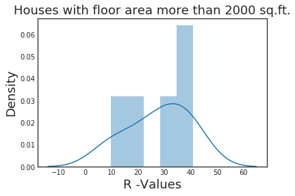
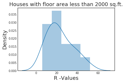
Figure 1. Distribution of R-values of houses

To investigate these shortcomings and their resolution, in this paper we present a systematic study of Bayesian approaches to the modeling of buildings’ thermal dynamics. We propose a generalized Bayesian State Space Model (BSSM) that can combine physics-based thermal models into a probabilistic framework. We further embed prior intuition and knowledge regarding buildings into the model based on subjective beliefs. For example, in Figure 1, the probability densities of the R-values of homes built before the year 2000 differ depending on their size, in this case whether their area is less than 2000 square feet. We show how to incorporate such knowledge by effective prior selection. However, such priors are not conjugate to the likelihood and solutions cannot be computed analytically. We thus perform inference based on algorithms that do not depend on conjugacy, such as Automatic Differentiation Variational Inference, and show that the buildings’ parameters can be estimated effectively with such an approximate approach. We analyze the effect of learning parameters from one season and use transfer learning to estimate the thermal dynamics in a different season when the HVAC is used in a different mode. We present two case studies on real data traces to show the effectiveness of the Bayesian approach, and the effects of prior selection and transfer learning across seasons.
Key Contributions: Our innovations and results provide evidence that the Bayesian approach to modeling a building’s thermal characteristics is valuable. The primary contributions of our work are as follows.

• Bayesian State Space Model: We propose a Bayesian state-space model for estimating buildings’ thermal parameters. Unlike previous methods (Bacher and Madsen, 2011; Juhl et al., 2017; Lazrak and Zeifman, 2017; Kristensen et al., 2004) which use point estimates, our Bayesian model is capable of incorporating beliefs using non-conjugate priors, and managing uncertainty in the parameters. We inferred the model parameters within a 95% credible interval with a Mean Field Variational Approximation, and show that the estimates are as accurate as that of a more time-consuming MCMC approach.

• Interpretable assessment of the generative model: We explored the generative characteristics of the model by Monte-Carlo simulation and forecasting, which helps understand the causal physical process that describes the thermal behavior of a house. We also tested the quality of the models by forecasting indoor temperature with the learned building parameters.

• Effects of transfer learning & prior selection: We proposed a transfer learning based approach by learning buildings’ parameters in summer, when HVAC is typically operational in cooling mode, and used it to aid fitting the data in seasons when HVAC is not used or operates in heating mode. We propose a systematic approach to prior selection to incorporate beliefs about the buildings’ characteristics in the model and conducted rigorous experiments to study their behavior.

The rest of the paper is structured as follows. In Section 2 we discuss related work on building parameter identification and Bayesian estimation. In Section 3 we propose the Bayesian State Space model for building parameter identification. In Section 4 we present two case studies and provide analysis of the model and finally conclude in Section 5.

2. Related Works

In this section, we review the previous works in three major related areas – parametric modeling of buildings’ thermal dynamics, techniques for parameter estimation, and a brief review of techniques for Bayesian inference.
Parametric modeling of buildings’ thermal dynamics helps to understand a building’s quality with few parameters. There are three approaches for modeling buildings’ thermal dynamics – White-box, Black-box and Gray-box modeling. White-box approach models all physical processes of a building (Hong et al., 2000; Kircher and Zhang, 2015) by formulating exact system dynamics. Such deterministic models are difficult to construct as the exact dynamics are often unavailable and due to the presence of noise in the data, arising from unaccounted factors. Black-box modeling approaches, such as regression, neural networks etc., are applied to model indoor temperature as a function of observed data, much like outdoor temperature (Nielsen et al., [n. d.]). However they do not describe the generative process and thus isn’t effective for interpretation. A gray-box model is a combination of prior physical knowledge and statistical approaches. The heat dynamics of the building was formulated using several equivalent models of varying complexity in (Bacher and Madsen, 2011), that estimated the insulation and the thermal mass of a building. An extension of such an approach included the effect of wind speed on infiltration is proposed in (Lazrak and Zeifman, 2017), and expansionary effect of air with temperature changes was modeled in (Siemann, 2013).
Parameter estimation for the gray-box model was performed in (Kristensen et al., 2004) by maximum likelihood estimation (MLE) and maximum a posteriori estimation (MAP). An extension of the approach (Ghosh et al., 2015), chose a simpler model to represent the dynamics and learned the residuals separately with Gaussian priors. Other works have focused on optimization based techniques (Reddy et al., 2007; Lazrak and Zeifman, 2017), where the objective is to minimize deviation between measurements and predictions from the model. Although, these approaches are simpler, they do not incorporate noise estimation in the equations. Alternatively, a Bayesian approach offers a natural way of dealing with parameter uncertainty in a state space model (Gordon et al., 1993; Geweke and Tanizaki, 2001). Bayesian methods have been widely used for the closely related problem of building energy modeling  (Li et al., 2016; Heo et al., 2012; Kim et al., 2013; Kristensen et al., 2017), but have been less well studied in the context of thermal modeling for buildings (Bacher and Madsen, 2011; Rouchier et al., 2018). A majority of previous works have applied the Metropolis-Hastings algorithm for Bayesian inference  (Rouchier et al., 2018; Heo et al., 2012; Kim et al., 2013; Li et al., 2016; Kristensen et al., 2017) which is ill-fitted for the specific problem as it takes a large number of steps to achieve convergence. The No U-Turn sampler (NUTS) showed better results (Chong et al., 2017) for parameter estimation in a related problem, building energy models, so we choose the latter.
Bayesian Inference, as performed in the previous works, used uninformed uniform priors and/or Normal priors for the model parameters (Bacher and Madsen, 2011; Rouchier et al., 2018). Such assumptions do not hold true as the parameters typically have non-Normal distributions. Non-normal priors do not have conjugacy with the likelihood, and analytical solutions of the posterior distribution are not possible. In such cases, algorithms that do not rely on conjugacy become important such as MCMC and Variational Inference. MCMC algorithms are capable of overcoming this problem but are time-consuming. Alternatively, Variational Inference (Beal et al., 2003; Luttinen, 2013) is an approximate inference that derives a lower bound for the marginal likelihood which can be optimized using stochastic gradient descent. In our experiments, we use the Mean Field Variational Inference and find that it provides similar parameter estimation to MCMC algorithms.

3. Proposed Approach

We follow the iterative modeling approach known as Box’s loop (Blei, 2014), shown in Fig. 2, for estimating buildings’ thermal parameters. The process starts with a collected and pre-processed dataset. We propose a Bayesian state space model to frame the problem and estimate parameters using MCMC and Variational Inference. Finally, we test for model convergence and measure the goodness of fit.

Figure 2. Box’s Loop

3.1. Bayesian Linear State Space Model

The generalized linear state space models consist of a sequence of $M$-dimensional observations ($y_{1}$, $y_{2}$, … $y_{N}$), assumed to be generated from latent $D$-dimensional states $X$ = ($x_{1}$, $x_{2}$, … $x_{N}$) and control variables $U$ = ($u_{1}$, $u_{2}$, … $u_{N}$). The data $Y$ is generated by the following state space equations:

(1) $$x_{n}=Ax_{n-1}+Bu_{n-1}+\mathcal{N}(0,Q)$$

(2) $$y_{n}=Cx_{n}+\mathcal{N}(0,R)\mbox{ ,}$$

where Eqn. 1 is the state evolution equation (analogous to HMM state transition) and Eqn. 2 is the observation or measurement equation (emission probability). The overall state transition probability is given as

$$P(X|A,B)=\mathcal{N}(x_{0}|m_{0},\Lambda_{0}^{-1})\times$$

(3) $$\prod_{i=1}^{N}\mathcal{N}(x_{n}|Ax_{n-1}+Bu_{n},diag(\tau_{1}^{-1}))\mbox{ ,}$$

where $x_{0}$ is an auxiliary initial state with mean $m_{0}$ and a precision matrix of $\Lambda_{0}$ (the matrix inverse of the covariance matrix). The emission probability is given by

(4) $$P(Y|C,X,\tau)=\prod_{n=1}^{N}\mathcal{N}(y_{n}|Cx_{n},diag(\tau^{-1}))\mbox{ .}$$

Here $Y$ is a normal distribution with mean CX and a covariance matrix with $diag(\tau^{-1})$. The covariance matrix R is a diagonal matrix as the noise is independent of the observed states $Y$. The graphical nature of the BSSM model is shown in Fig 3, which is analogous to an Input-Output HMM (Bengio and Frasconi, 1995).

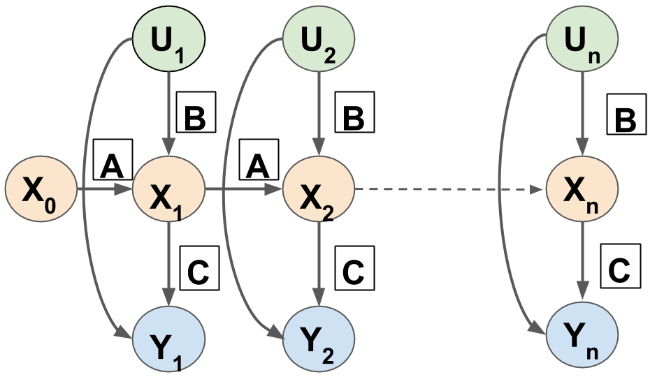
Figure 3. Bayesian State Space Model

3.2. Problem Formulation

We use an example to illustrate how to formulate a building’s thermal equations and incorporate them into the proposed state space model framework. Figure 4 shows an equivalent circuit that describes the thermal dynamics of a house.

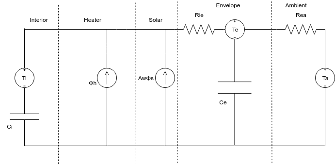
Figure 4. TiTe circuit model

In this example, called the $TiTe$ model, we assume that there are two latent state spaces $Ti$ and $Te$ that describes the indoor and envelope temperatures. The thermal dynamics is represented by a set of stochastic differential equations derived from the equivalent assumption. The equations of the process are given by:

(5) $$dT_{i} =\frac{1}{R_{ie}C_{i}}(T_{e}-T_{i})dt+\frac{1}{C_{i}}\Phi_{h}dt+\frac{A_{w}}{C_{i}}\Phi_{s}dt+\sigma_{i}d\omega_{i}$$

(6) $$dT_{e} =\frac{1}{R_{ie}C_{e}}(T_{i}-T_{e})dt+\frac{1}{R_{Bea}C_{e}}(T_{a}-T_{e})dt+\sigma_{e}d\omega_{e}$$

(7) $$Y_{k} =T_{i_{k}}+e_{k}\mbox{ ,}$$

where t is the time, $R_{ie}$ is the thermal resistance between the interior and the building envelope, $R_{ea}$ is the thermal resistance between the building envelope and the ambient air, $C_{i}$ is the heat capacity of the interior, $C_{e}$ is the heat capacity of the building envelope, $\Phi_{h}$ is the energy flux from the heating system, $A_{w}$ is the effective window area, $\Phi_{s}$ is the energy flux from solar radiation, $T_{a}$ is the ambient air temperature, $\{\omega_{i,t}\}$ and $\{\omega_{e,t}\}$ are standard Wiener processes with variances $\sigma_{i}$ and $\sigma_{e}$ respectively, where $t$ is the point in time of a measurement. $Y_{t}$ is the indoor temperature, $T_{i_{k}}$ is the measured interior and $e_{k}$ is the measurement error, which is assumed to be a Gaussian white noise process. Converting the differential equations (Eqns 5–7) as difference equations we get the transition and emission matrix form as:

$$\begin{bmatrix}Ti(t+1)\\ Te(t+1)\end{bmatrix} =\begin{bmatrix}1-\frac{1}{R_{ie}C_{i}}&\frac{1}{R_{ie}C_{i}}\\ \frac{1}{R_{ie}C_{e}}&1-\frac{1}{R_{ie}C_{e}}-\frac{1}{R_{ia}C_{e}}\end{bmatrix}\times\begin{bmatrix}Ti(t)\\ Te(t)\end{bmatrix}$$

(8) $$+\begin{bmatrix}0&\frac{1}{C_{i}}&\frac{A_{w}}{C_{i}}\\ \frac{1}{R_{ia}C_{e}}&0&0\end{bmatrix}\times\begin{bmatrix}Ta(t+1)\\ \Phi_{h}(t+1)\\ \Phi_{s}(t+1)\end{bmatrix}+\begin{bmatrix}\sigma_{i}&0\\ 0&\sigma_{e}\end{bmatrix}$$

(9) $$Y(t) =\begin{bmatrix}1&0\end{bmatrix}\times\begin{bmatrix}Ti(t)\\ Te(t)\end{bmatrix}+\sigma\mbox{ .}$$

Eqn 8 is the state transition of the dynamic system and is equivalent to the general form as presented in Eqn 1 that gives us the transition probability, i.e $P(x_{t+1}|x_{t})$ $\sim$ $\mathcal{N}(AX+BU,\Sigma_{w})$ (Eqn 3). Similarly, Eqn 9 is equivalent to the measurement equation provided by Eqn 2 that gives us the emission probability (Eqn 4). In Eqn 8, the first two matrices models the physical dynamics and the third matrix is the measure of stochasticity in the data. Similarly, in Eqn 9, the first matrix is the measurement equation and $\sigma$ is the error in measurement. In the base case, we assume an uninformative Gamma prior over the model parameters and the hyper-parameters of the gamma distribution are automatic relevance determination (ARD) parameters, which prune out components that are not significant enough. We provide broad priors to the gamma distribution by setting the shape and rate to a very small value (Beal et al., 2003). Thus parameters are given as $\mathbf{R}\sim\Gamma(\alpha=\delta,\beta=\delta)$, $\mathbf{C}\sim\Gamma(\alpha=\delta,\beta=\delta)$, $\mathbf{Aw}\sim\Gamma(\alpha=\delta,\beta=\delta)$, where $\delta$ is a very small value. We also impose a bound on the parameters, which can help by limiting the parameters to certain reasonable ranges. We formulate other instantiations of the physical models in the case studies presented in Section 4.1.2.

3.3. Bayesian Inference

Bayesian inference recovers the posterior distribution over parameters and latent variables of the model, which can hence be used to perform prediction. While exact solutions can be achieved for some basic models, computing the posterior distribution is generally an intractable problem, in which case approximate inference is needed.
Markov chain Monte Carlo (MCMC) algorithms are a widely applied method for approximate inference, which aims to estimate the posterior using a collection of samples drawn from an appropriate Markov chain. Hamiltonian Monte Carlo (HMC) (Neal et al., 2011) algorithms such as NUTS avoid the random walk behavior by taking a series of steps informed by first-order gradient information. These features allow it to converge to high-dimensional target distributions much more quickly than simpler methods such as random walk Metropolis Hastings (Yildirim, 2012). The No U-Turn Sampler (NUTS) (Hoffman and Gelman, 2014) uses a recursive algorithm to build a set of likely candidate points that span a range of the target distribution, stopping automatically when it starts to backtrack and retrace its steps, which prevents the revisiting of previously explored paths. In this work, we select the NUTS sampler for inference.
Another option is Variational Inference, which is a class of algorithms that are deterministic alternatives to MCMC. This reduces inference tasks to an optimization problem (Blei et al., 2017). In a probabilistic latent model setting, Y is the observed data, X is the latent variable space and $\theta$ the model parameters. An approximating distribution $q(X,\theta)$ over the latent variables and parameters, called the variational distribution, is constructed to approximate the posterior. The objective is to reduce the “gap” between the variational and the posterior distribution. This gap is given by the Kullback-Leibler divergence, which is the relative entropy between the two distributions, given as:

$$KL(q(X,\theta)||p(X,\theta|Y))=\mathbb{E}_{q}\Big{[}log\>\frac{q(X,\theta)}{p(X,\theta|Y)}\Big{]}$$

(10) $$=\mathbb{E}_{q}[log\>q(X,\theta)]-\mathbb{E}_{q}[log\>p(X,\theta,Y)]+log\>p(Y)\mbox{ .}$$

In Eqn 3.3, $log\>p(Y)$ is independent of the distribution $q(X,\theta)$, so minimizing Eqn 3.3 is equivalent to maximizing:

$$\mathbf{L}(q)=\mathbb{E}_{q}[log\>p(X,\theta,Y)]-\mathbb{E}_{q}[log\>q(X,\theta)]$$

(11) $$=\mathbb{E}_{q}[log\>p(X,\theta,Y)]+H(q)\mbox{ .}$$

Using Jensen’s inequality, $\mathbf{L}(q)$ can be shown to be a lower bound on $\log\>p(Y)$, and is hence known as the Evidence Lower Bound (ELBO). To make inference tractable, we make simplifying assumptions on $q$. The most commonly used assumption is the mean-field approximation, which assumes that the latent variables are independent of each other. Thus the variational distribution with $N$ latent variables is assumed factorized as $q(X,\theta)=q(\theta)\prod_{i=1}^{N}q(X_{i})$. Traditionally, a Variational Inference algorithm requires developing and implementing model specific optimization routines. Automatic Differentiation Variational Inference (ADVI) (Kucukelbir et al., 2017) proposes an automatic solution to posterior inference. ADVI first transforms the model into one with unconstrained real-valued latent variables. It then recasts the gradient of the variational objective function as an expectation over q. This involves the gradient of the log of the joint likelihood with respect to the latent variable $\bigtriangledown_{\theta}\;log\;p(x,\theta)$, which is computed using reverse-mode automatic differentiation (Maclaurin, 2016). This gradient term is applied to optimize the parameters using a stochastic gradient descent approach.
It is important to note the underlying assumptions of ADVI. It factors the posterior distribution such that all the state variables are statistically independent, following the mean-field approximation. For a highly correlated posterior, e.g. in state space models, where the intuition is that $x_{t+1}\sim N(x_{t},\theta)$ will be highly correlated with $x_{t}$, the mean-field assumption is rather unrealistic. The method can still work well in practice, however, as the (uncorrelated) $q$ is fit to the (correlated) $p$, thereby exploiting dependencies, even though they are not ultimately encoded in $q$. NUTS, on the other hand, is very good at exploring a correlated, high-dimensional distribution, but can suffer in both run-time and convergence speed versus ADVI. We empirically evaluate the effectiveness of these approximations by comparing the parameters inferred by both the methods.

3.4. Model Criticism

Model criticism requires tests for convergence and testing goodness of fit on held out data. Since the primary objective of the study is to obtain the estimated parameter values, we also inspect the credible interval of the parameters. If the region is too wide we infer that the uncertainty in estimation is high.
Convergence Diagnostics: We select the Gelman-Rubin diagnostic (Gelman et al., 2011), which checks for the lack of convergence by comparing the variance between multiple chains to the variance within each chain. Convergence is more straightforward to analyze for Variational Inference. The convergence criterion is simply to iterate until the ELBO no longer increases.
Goodness of fit is tested using posterior predictive checks, which are performed by simulating replicated data under the fitted model and then comparing these to the observed data to look for systematic discrepancies between real and simulated data (Gelman et al., 2013).
Credible Interval: The motivation behind using a Bayesian approach is to find the range of possible values for the building parameters. A standard measure of confidence in some (scalar) quantity $\theta$ is the “width” of its posterior distribution. This can be measured using a 100(1 - $\alpha$)% credible interval, where we select $\alpha$ as 0.05 to estimate parameters with a 95% probability,

(12) $$C_{\alpha}(D)=(l,u):P(l\leq\theta\leq u|Y)=1-\alpha\mbox{ ,}$$

where the interval for a parameter is bounded by (l,u) with a probability $1-\alpha$. The credible interval is a Bayesian alternative to a frequentist confidence interval. A frequentist keeps the parameters fixed and varies the confidence interval whereas a Bayesian approach is to keep the credible region fixed and vary the model parameters.

3.5. Application of the Models

3.5.1. Exploration

In terms of building modeling, we are primarily interested in learning the different R and C parameters. As we consider different multi-state lumped models, the cardinality of the sets R and C may vary but the overall values should remain the same. To find the composite resistance of the equivalent circuit, the resistance and capacitance are obtained by Kirchoff’s law. However, the simple addition or geometric sum required to compute the composite parameters cannot straightforwardly be done as Bayesian Inference provides random variables rather than scalar quantities. The distribution of the sum of two random variables can be obtained by the convolution of their density functions.

Algorithm 1 Indoor Temperature Forecast

1:procedure Forecast (Input: Distribution of the model parameters $\theta=\{\mathbf{R},\mathbf{C},\mathbf{A},\mathbf{X}_{T}\}$, time window of forecast $K$)

2:     Set start temperature state to $X_{T}$

3:     {$R_{i}$ , $C_{i}$, $A_{i}$} ¡- Draw N Sample(R, C, A)

4:     for i in 1 : N do

5:         $X^{(i)}_{T+1:T+K}$ $\leftarrow$ $BSSM(X_{T},R_{i},C_{i},A_{i})$

6:     end for

7:     Mean Prediction $\leftarrow$ $\mathbf{E}\{X^{(i)}_{T+1:T+K}\}$

8:     Credible Interval $\leftarrow$ {$Max(X^{(i)}_{T+1:T+K})$ , $Min(X^{(i)}_{T+1:T+K})$}

9:end procedure

3.5.2. Forecasting

We perform 24 hour ahead forecast, after learning the parameters of the model. We assume that a outdoor temperature forecast data is given to us and we assumed that the HVAC is operational in the last known mode. The forecasting and prediction of HVAC time is given in Algorithm 1. When the HVAC is set to a particular temperature and assuming that it is not changed within the horizon of the forecast, then the indoor temperature will be centered around the set-point in a range known as the thermostat hysteresis setting. In general, the range is $\pm$ $\delta$ lies within 0.5 – 1 ^∘F. We sample from the estimated parameters’ distributions to obtain the forecasting interval.

3.6. Implementation

We implemented the Bayesian State Space model using the PyMC3 probabilistic programming library in Python (Salvatier et al., 2016). PyMC3 is built on Theano (Theano Development Team, 2016) and has built-in implementations for MCMC algorithms and Variational Inference methods. We formulated the different components of the state space model and set the prior distributions for the model parameters. We deployed our methods on a system with 16 GB RAM system and I7 processor. The initial version of the codes is available in the BSSP Github repository.

Table 1. Results of Study I

Model	Method	Total R	Total C	Ria	Rie	Rih	Rea	Ci	Ce	Ch	Aw	Ae	NRMSE (%)	RMSE	Convergence Time (Steps)
Ti	EKF	5.29	24.797	5.29	-	-	-	2.06	-	-	7.89	-	0.4	0.06	2.68s ( Steps = 39)
	MCMC	5.29, 0.06	24.96, 0.36	5.29, 0.06	-	-	-	24.96, 0.36 -	-	-	7.95, 0.675	-	0.8	0.10	30 min (Chains = 4, Steps = 5000)
	ADVI	5.29, 0.67	24.75, 0.40	5.29, 0.067	-	-	-	24.73, 0.43	-	-	7.87, 0.675	-	0.4	0.05	2.26min (Steps = 180000)
TiTe	EKF	5.36	39.17	-	5.17	-	0.19	19.99	19.18	-	23.78	-	0.3	0.04	14.65s (100)
	MCMC	5.27, 0.17	89.95, 7.92	-	1.73, 0.056	-	3.54, 0.122	21.39, 0.30	68.56, 7.91	-	10.75, 0.64	-	0.3	0.04	1.5 hrs (4,5000)
	ADVI	5.29, 0.002	25.31, 0.86	-	1.98, 0.001	-	3.31, 0.002	24.49 , 0.502	0.82, 0.008	-	7.90, 0.86	-	0.3	0.04	2:38 min (Steps = 180000)
TiTeTh	EKF	-	-	-	-	-	-	-	-	-	-	-	-	-	No Convergence
	MCMC	-	-	-	159.13, 273.83	70.23, 159.81	23.08, 68.44	119.77, 206.30	121.85, 184.87	313.33, 342.47	15.52, 28.71	0.092, 0.60	-	-	No Convergence
	ADVI	2.8, 0.004	184.45, 13.58	-	2.176, 0.010	0.23, 0.003	0.63, 0.003	177.82, 83.22	2.05, 0.03	4.59, 0.097	52.76, 193.86	45.50, 181.90	-	-	4.23min (Steps = 180000)

4. Analysis

In this section we provide two case studies. In the first test case we compare the results with small dataset to contrast and compare the gray-box models’ solutions with the Kalman filter and Bayesian state space model. In the second case study, we present results and analyses on larger scale data from the Dataport Dataset (Pec, [n. d.]).

4.1. Case Study I: Exploratory Study on a Benchmark Dataset

4.1.1. Dataset

We compare the results with the benchmark dataset provided in (Bacher and Madsen, 2011) and the circuit assumptions of the house mentioned in the paper. The data is from a Flexhouse in Risø DTU in Denmark, and was collected during a series of experiments carried out in February to April 2009, where measurements consist of five minute values over a period of six days. The dataset consist of a single signal representing the indoor temperature ($y$ ^∘C). Observed ambient air temperature at the climate station ($Ta$ ^∘C). Total heat input from the electrical heaters in the building ($\Phi_{h}$ kW). The global irradiance was measured at the climate station ($\Phi_{s}$ kW/$m^{2}$).

4.1.2. Problem Formulation

First we constructed all the models suggested in (Bacher and Madsen, 2011). The CTSM (Kristensen and Madsen, 2003) package can be used to model Continuous Time Stochastic Processes which is realized using an Extended Kalman Filter (EKF). We define R, C, and A to be the set of resistances, capacitances and area of solar infiltration for individual models. The three models which we chose for inspection and their system dynamics as follows:

• Ti Model: Here the house as a whole is assumed to have one thermal resistance ($R_{ia}$) and capacitance ($C_{i}$).

  $$T_{i}(k+1) =(1-\frac{1}{R_{ia}C_{i}})\times T_{i}(k)+\frac{1}{R_{ia}C_{i}}\times T_{e}(k+1)$$

  (13) $$+\frac{1}{C_{i}}\times\Phi_{h}(k+1)+\frac{A_{w}}{C_{i}}\Phi_{s}(k+1)+\sigma_{i}$$

  (14) $$Y_{k} =T_{i}(k)+e_{k}$$

• TiTe Model: We provided a detailed description of formulation using the TiTe model in Section 3.2.

• TiTeTh Model: The three state model represents the interior subscripted by i, the exterior subscripted by e and the heater subscripted by h. The formulation for the three states are as follows:

  $$T_{i}(k+1) =(1-\frac{1}{R_{ie}C_{i}})\times T_{i}(k)+\frac{1}{R_{ie}C_{i}}\times T_{e}(k+1)$$

  (15) $$+\frac{A_{w}}{C_{i}}\times\Phi_{s}(k+1)+\sigma_{i}$$

  $$T_{e}(k+1) =(1-\frac{1}{R_{ie}C_{e}}-\frac{1}{R_{ea}C_{e}})\times T_{e}(k)+\frac{1}{R_{ea}C_{e}}\times T_{a}(k+1)$$

  (16) $$+\frac{1}{R_{ie}C_{e}}\times T_{i}(k+1)+\sigma_{e}$$

  $$T_{h}(k+1) =(1-\frac{1}{R_{ih}C_{h}})\times T_{h}(k)+\frac{1}{R_{ih}C_{h}}\times T_{i}(k+1)$$

  (17) $$+\frac{1}{C_{h}}\times\Phi_{h}(k+1)+\sigma_{h}$$

  (18) $$Y_{k} =T_{i}(k)+e_{k}$$

4.1.3. Results Discussion

We show the results of the first case study in Table 1. We provide the mean and variances ($\mu$, $\sigma$) of the estimated model parameters – R, C and Aw, within a 95% credible interval range as shown in Table 1. The total R and total C the composite thermal resistance and capacitance of the building. We compare the results of Bayesian Inference with the point estimates with an Extended Kalman Filter (EKF). The insights from the study are as follows:
Estimated model parameters: From the Table 1 we found that the mean of the credible interval for the estimated parameters for the Bayesian approaches is similar to that of the EKF point estimate. The EKF assumes the parameters to have uniform priors and thus performs MLE for estimation. An approximate ADVI provides a similar parameter estimation as that of an equivalent run of MCMC inference.
Comparison with the point estimates: A direct comparison of the model’s performances between the Bayesian methods and the EKF is difficult. We take the mean of the parameter estimated from Bayesian inference and then perform a one-step-ahead prediction and compare that with the EKF. The metrics used for comparison are the root mean squared (RMSE) and the normalized root mean squared errors (NRMSE) of the one-step-ahead prediction and we find that estimates from ADVI give us the best results (Table 1).
Time of execution to reach convergence: MLE estimates of the EKF is the fastest as it does not require computation of the full posterior distribution, however, it does not provide estimation error over model parameters. The MCMC algorithm is the most time consuming one, where we increase the number of steps and check for convergence using Gelman-Rubin diagnostic. We selected 4 chains and an initial burn in 5000 steps which is intended to give the Markov Chain time to reach its equilibrium distribution when there is a random initial starting point. Compared to MCMC, ADVI is much faster. For the $TiTeTh$ model, we obtain no convergence for the EKF or MCMC, i.e. the credible intervals are very wide. But ADVI provides reasonable intervals for some parameters. We listed the time of execution for the different approaches in Table 1.

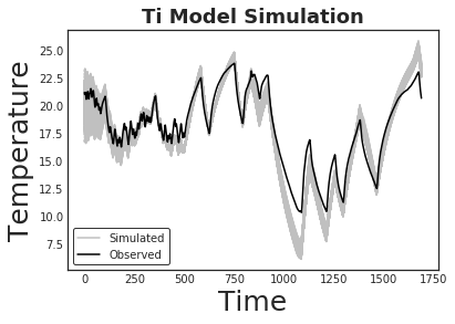
(a) Ti model

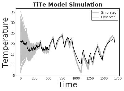
(b) TiTe model

Figure 5. Monte Carlo Simulation of Indoor Temperature

Monte-Carlo simulation: We perform a Monte-Carlo simulation to generate the possible indoor temperature scenarios when weather and HVAC usage is provided. In Figure 5 we show the results of the simulated prediction for the Ti and TiTe models, drawing samples from the inferred parameter distributions. We considered the starting state to be drawn from a $\mathbb{N}$(70, 5) distribution, i.e. our guess for the indoor temperature will be within the range of 60 - 80^∘F. The simulated prediction shows that the actual value of the indoor temperature is enclosed within the credible region. It, however, deviates in certain sections, which we hypothesize is because the thermal mass of a house can change with varying temperature. The RC constant (Boylestad et al., 2002) of the data changes with time as the thermal mass C of a house can vary, due expansion (or contraction) of air. A more generalized formulation of thermal dynamics will require exploring longitudinal studies that to correlate between the parameter and temperature changes with the heater and cooler usage for long duration.

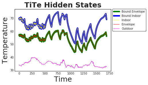
(a) Hidden States of TiTe model

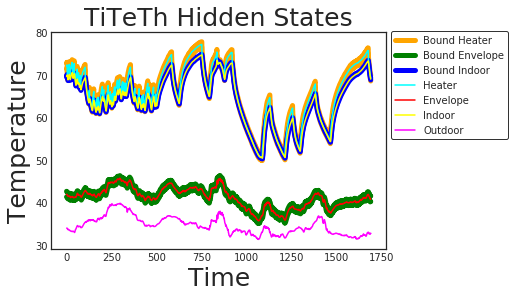
(b) Hidden States of TiTeTh model

Figure 6. Visualizing Hidden State Dynamics

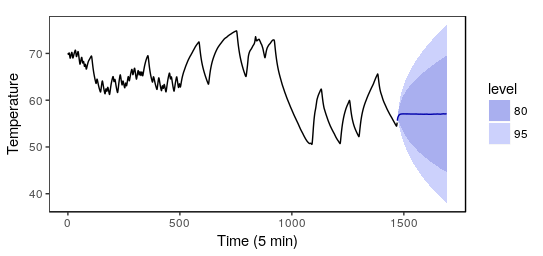
(a) ARIMAX

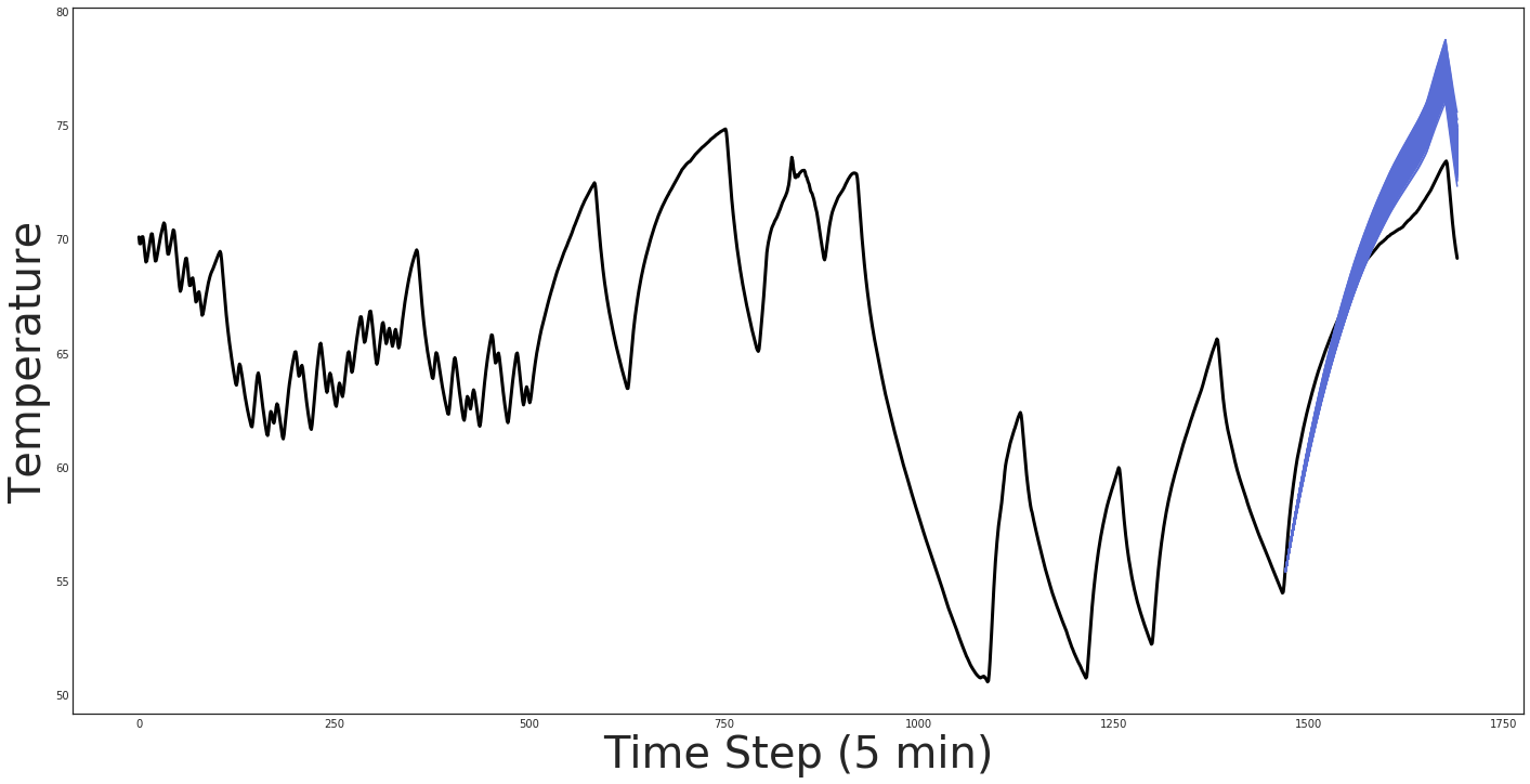
(b) Ti Model

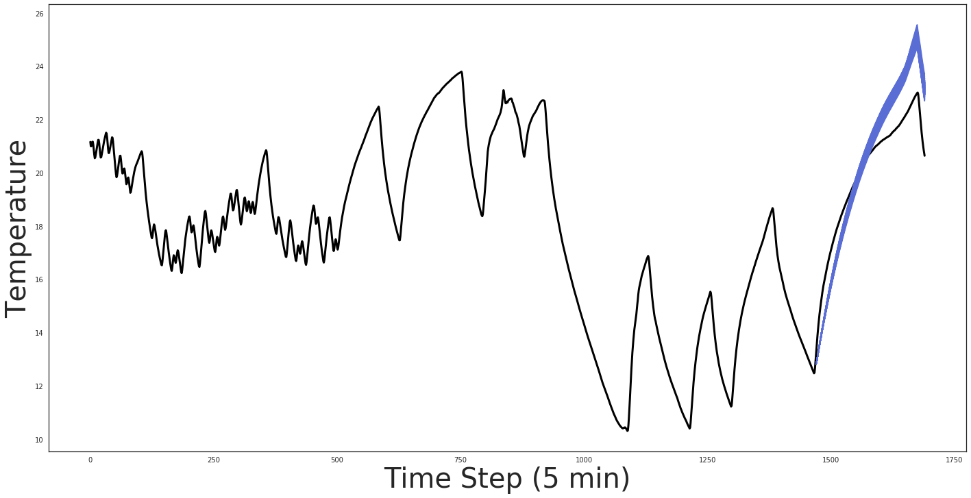
(c) TiTe Model

Figure 7. Comparison of Forecasting

Qualitative assessment of the hidden states: In Figure 6, we show the learned hidden states of the two-state $TiTe$ and three state $TiTeTh$ model. For the $TiTe$ model shown in Fig 6(a), show that the estimated hidden state for the envelope is sandwiched between the indoor temperature and the outdoor temperature and is more correlated with the indoor temperature. Whereas in the $TiTeTh$ model (Fig 6(b)) the envelope state is more correlated with the outdoor temperature. However, the heater’s temperature is the same as that of the indoor temperature, which implies it does not capture an independent factor of the hidden state space. The plots in Fig 6 show the error margin of the hidden states obtained from the highest posterior distribution.

Forecasting: We compared the forecasting results of the BSSM with an auto-regressive integrated moving average with exogenous variables (ARIMAX). We used the first 5 days for training the BSSM and learn the building parameters. We then used the learned parameters to obtain a day ahead forecast within 95% prediction interval, as presented in Algorithm 1. Our assumption is that the heater stays in the same state as the last known state and assumed that the solar radiation and temperature data are available. In Figures 7(a) – 7(c) we show the output of forecasting for the ARIMAX, $Ti$ and $TiTe$ models. For quantitative evaluation we chose the mean absolute percentage error (MAPE) to find the error in mean of the forecast and calculated the percent of data within 95% forecast interval as shown in Table 2. The mean forecast error is lower in case of the BSSM models as they better learn the dynamics of the process. However, as the model parameters have a narrow credible interval, the actual data lies outside the forecast interval in but provides a narrower band for which the actual value partially lies outside the credible interval. In contrast, the forecasting result of ARIMAX has less correlation, although the actual forecast is within the confidence interval.

Table 2. Results of Forecasting

Method	MAPE	% of data within 95%
		forecast interval
ARIMAX	0.19	100%
Ti Model	0.05	78%
TiTe Model	0.04	79%

4.2. Case Study II: Prior Selection & Transfer Learning

4.2.1. Dataset

The Dataport dataset is a publicly available dataset, created by Pecan Street Inc, which contains building-level electricity data from 1000+ households. We performed our experiments on three single-family homes from Texas (dataid = 484, 739, 1507) based on metadata availability and proper registration of indoor temperature and HVAC usage data. The metadata, which has information about 52 homes, provides a general understanding about the buildings and helps us create prior distributions over the R-values. Here, House 739 does not have heating data available and the metadata does not include a measure for House 1507’s R-value.

4.2.2. Experimental setup

In this case study we explore the effects of prior selection and transfer learning. The two processes are inherently tied together, since in the Bayesian approach, “today’s posterior becomes tomorrow’s prior.” Our approach here is to learn the parameters from the AC usage season, where data is more consistent, and transfer the learned parameters as priors to seasons when HVAC has typically no usage and/or operates in heating mode. We investigate the effect of three sets of priors:

• Informed Priors (Set 1): We selected informed gamma priors. This is useful when we have some notion about the parameters’ values such as an initial audit to estimate the R-value of a building. We select a strong prior on the R-value where the mean of the R-value is same as that of the estimate and the standard deviation is 1.

• Hyper Priors (Set 2): In this set, we don’t have a direct estimation regarding the buildings’ parameters but have a vague understanding about the expected value from the metadata. We encode such beliefs by setting a hyper-prior for the mean, that is sampled selected from a mixture of lognormal distributions. We empirically found that R-values are a mixture of lognormal distributions, conditioned on the year built and conditioned square foot, by performing a maximum likelihood estimate. The estimated parameters of the two lognormal distributions as shown in Fig 1, are ($\mu_{0}$, $\sigma_{0}$) = (3.02, 0.59) and ($\mu_{1}$, $\sigma_{1}$) = (3.43, 0.50), respectively.

• Uninformed Priors (Set 3): Finally, in Set 3, we chose uninformed flat gamma priors for the R-values, where, we have no knowledge of the buildings’ parameters. In all three cases we set a flat gamma prior on the C-values.

Table 3. Results of Case Study II

Homes	HVAC Mode	R-Value	Informed Priors		Hyper Priors		Uninformed Priors
			R	C	R	C	R	C
	No Usage		26, 0.02	85.92, 12	53.24, 14.99	81.6, 10.86	449.04, 431.90	80.82 , 10.71
484	AC	26	26, 0.02	85.03 , 12.5	52.12, 15.33	80.81, 11.08	453.73, 428.96	80.25, 10.99
	Heater		26, 0.02	132.44 , 12.79	75.87, 15.9	89.35, 11.7	343.63 , 276.16	81.48 , 11.73
	No Usage		6.1, 0.23	73.15, 18.84	61.82, 14.46	15.43, 1.945	62.1 , 14.33	15.33, 2.005
739	AC	6	6.1, 0.23	64.09, 20.7	58.88, 10.87	15.55, 1.79	59.47, 10.43	15.65, 1.84
	Heater		-	-	-	-	-	-
	No Usage		-	-	24.52, 0.215	103.4, 7.34	48.66, 20.91	107.42, 7.56
1507	AC	NA	-	-	23.58, 0.215	103.52, 7.89	47.65, 21.95	107.88, 7.55
	Heater		-	-	23.58, 0.23	104.65, 8.79	52.22, 26.62	108.84, 8.38

For all three cases, we set an upper bound on the R-values to be 70, which we found from the metadata. We assign an uninformed gamma prior on the C values. For all cases, we initially estimate for the AC usage scenario and use the mean and variance of the estimated parameters to set the prior for the other seasons. The sign of the heat flux, as provided in Eqn 8, is negative when AC is used and the HVAC is in cooling mode. We do not have an exact value for heater’s flux but we use the furnace which provides the binary “ON-OFF” signal of the heater and multiply an extra unknown parameter $\Phi_{h}$ to estimate the heat flux. Similarly to the previous section, we estimate all parameters within a 95% credible interval. We also varied the size of the dataset of sizes [200, 500, 1000, 2000, 5000].

4.2.3. Results

The prior selection directly influences the value of the parameters, parameter transfer and depends on the size of the dataset. A summary of the results is presented in Table 3 for 2000 data points, which provides us the most likely parameter estimates. We present the result in the form of mean and the error margins i.e. ($\mu$, $\pm\epsilon$). We find that the Informed Priors provide us with the most consistent estimates both across size of the datasets and when we perform transfer learning. As shown in Fig 8, the informed parameters remain consistent with the change in the size of the dataset with very little margin of error ($\pm$ 1). Parameter transfer also works best when informed priors are applied (Fig 8), but can provide us different estimates when being transferred from AC usage to Heater usage seasons. The hyper-priors reduce the margin of error when applied for smaller datasets. For example, in Fig 10, the R-values have large error margins when uninformed priors are chosen, which is significantly reduced when hyperpriors were used Fig 9.

4.2.4. Discussion

Information in the data overwhelms prior information not only when the size of the dataset is large, but also when the prior encodes relatively small information. For example in House 739 (Table 3), an approach using uninformed priors will try to get the best estimate that fits the data, but the parameters may not be accurate. For this case, a sharp prior centered around an initial estimate gives the best result. Uninformative priors are easily persuaded by data, while strongly informative ones may be more resistant. When the size of the dataset is small, hyperpriors effectively reduce the margin of error in parameter estimation Fig. 9.

4.3. General Recommendations

Based on our studies, we recommend constructing a Bayesian state space model customized for the problem at hand, carefully selecting the system dynamics and priors. We suggest using ADVI for parameter estimation as it provides similar estimates but is faster than MCMC. In realistic settings, it is better to perform an initial audit to determine the home’s insulation parameters and fix an informed prior on the parameter set. We suggest to use informative priors, if enough metadata is available to set them reliably. However, if the objective is to monitor a large set of homes, we recommend setting a hyper prior based on the beliefs from a sample of the dataset. If the heat flux is known from the HVAC, learning from one season and applying it to another can improve estimation.

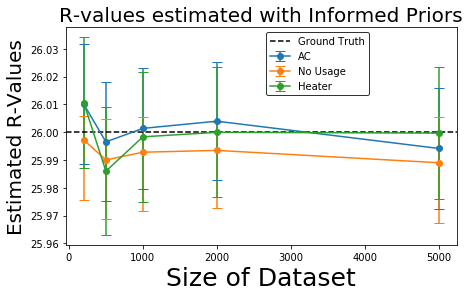
(a)

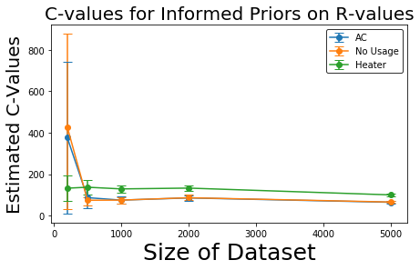
(b)

Figure 8. Informed Prior set on R-values

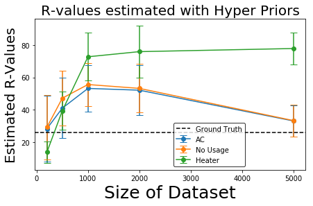
(a)

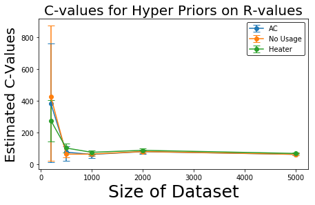
(b)

Figure 9. Hyper Prior set on R-values

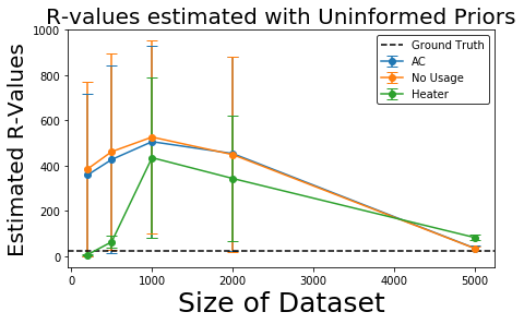
(a)

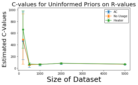
(b)

Figure 10. Uninformed set on R-values

These figures show the results of parameter estimation of R and C values for House 484 with varying data sizes and different prior selection.

5. Conclusion & Future Work

In this paper, we proposed and systematically studied Bayesian statistical approaches to buildings’ thermal parameter estimation. We developed a generalized state-space modeling framework that integrates building physics equations with a statistical model. The model estimates buildings’ structural parameters which influence the indoor temperature conditioned on HVAC usage and weather factors. We contrast model learning using MCMC and ADVI algorithms and show that Variational Inference is faster and provides a similar estimation to MCMC. A visual inspection of the hidden states was employed to assess the model dynamics, and we found that merely increasing model complexity does not capture any significant factors of the thermal characteristics. We further showed the model’s applications, such as simulating probable outcomes and forecasting the future. The effects of prior selection on the parameter estimation were studied in detail. We found that informed priors provide the best estimates, but when such information is not present prior beliefs can help to better learn the models. Also, we found that priors are key to transfer learning, and model parameters learned from one season can be used to model thermal dynamics under the condition that properly scaled exogenous data is available.
The focus of our future research is in two directions. We are presently instrumenting several homes with smart thermostats and temperature sensors. This study serves as a guide to large-scale analysis as we attempt to further incorporate air leakages and construct room level thermal behavior analysis. We plan to learn from the data that is being collected longitudinally and incorporate the learned models in NEST thermostats to monitor homes’ condition continuously. Secondly, we will focus on incorporating air-leakage into the framework and correlating with standardized metrics such as $ACH_{50}$. Common air-infiltration models (e.g. LBL model (Sherman, 1992)), have complex non-linear characteristics for which we will explore non-linear state space models.

References

- (1)
- Pec ([n. d.]) [n. d.]. Source: Pecan Street Inc. Dataport 2018. ([n. d.]).
- EIA (2017) 2017. Annual energy outlook 2017. US Energy Information Administration (2017).
- Bacher and Madsen (2011) Peder Bacher and Henrik Madsen. 2011. Identifying suitable models for the heat dynamics of buildings. Energy and Buildings 43, 7 (2011), 1511–1522.
- Beal et al. (2003) Matthew James Beal et al. 2003. Variational algorithms for approximate Bayesian inference. University of London London.
- Bengio and Frasconi (1995) Yoshua Bengio and Paolo Frasconi. 1995. An input output HMM architecture. In Advances in neural information processing systems. 427–434.
- Blei (2014) David M Blei. 2014. Build, compute, critique, repeat: Data analysis with latent variable models. Annual Review of Statistics and Its Application 1 (2014), 203–232.
- Blei et al. (2017) David M Blei, Alp Kucukelbir, and Jon D McAuliffe. 2017. Variational inference: A review for statisticians. J. Amer. Statist. Assoc. 112, 518 (2017), 859–877.
- Boylestad et al. (2002) Robert L Boylestad, Louis Nashelsky, and Lihua Li. 2002. Electronic devices and circuit theory. Vol. 11. Prentice Hall Englewood Cliffs, NJ.
- Chong et al. (2017) Adrian Chong, Khee Poh Lam, Matteo Pozzi, and Junjing Yang. 2017. Bayesian calibration of building energy models with large datasets. Energy and Buildings 154 (2017), 343–355.
- Fabrizio and Monetti (2015) Enrico Fabrizio and Valentina Monetti. 2015. Methodologies and advancements in the calibration of building energy models. Energies 8, 4 (2015), 2548–2574.
- Gelman et al. (2011) Andrew Gelman, Kenneth Shirley, et al. 2011. Inference from simulations and monitoring convergence. Handbook of markov chain monte carlo (2011), 163–174.
- Gelman et al. (2013) Andrew Gelman, Hal S Stern, John B Carlin, David B Dunson, Aki Vehtari, and Donald B Rubin. 2013. Bayesian data analysis. Chapman and Hall/CRC.
- Geweke and Tanizaki (2001) John Geweke and Hisashi Tanizaki. 2001. Bayesian estimation of state-space models using the Metropolis–Hastings algorithm within Gibbs sampling. Computational Statistics & Data Analysis 37, 2 (2001), 151–170.
- Ghosh et al. (2015) Siddhartha Ghosh, Steve Reece, Alex Rogers, Stephen Roberts, Areej Malibari, and Nicholas R Jennings. 2015. Modeling the thermal dynamics of buildings: A latent-force-model-based approach. ACM Transactions on Intelligent Systems and Technology (TIST) 6, 1 (2015), 7.
- Gordon et al. (1993) Neil J Gordon, David J Salmond, and Adrian FM Smith. 1993. Novel approach to nonlinear/non-Gaussian Bayesian state estimation. In IEEE Proceedings of Radar and Signal Processing, Vol. 140. IET, 107–113.
- Gouda et al. (2002) MM Gouda, Sean Danaher, and CP Underwood. 2002. Building thermal model reduction using nonlinear constrained optimization. Building and environment 37, 12 (2002), 1255–1265.
- Heo et al. (2012) Yeonsook Heo, Ruchi Choudhary, and GA Augenbroe. 2012. Calibration of building energy models for retrofit analysis under uncertainty. Energy and Buildings 47 (2012), 550–560.
- Hoffman and Gelman (2014) Matthew D Hoffman and Andrew Gelman. 2014. The No-U-turn sampler: adaptively setting path lengths in Hamiltonian Monte Carlo. Journal of Machine Learning Research 15, 1 (2014), 1593–1623.
- Hong et al. (2000) Tianzhen Hong, S.K Chou, and T.Y Bong. 2000. Building simulation: an overview of developments and information sources. Building and Environment 35, 4 (2000), 347 – 361.
- Juhl et al. (2017) Rune Juhl, Niels Rode Kristensen, Peder Bacher, Jan Kloppenborg, and Henrik Madsen. 2017. Grey-box modeling of the heat dynamics of a building with CTSM-R. (2017).
- Kim et al. (2013) Young-Jin Kim, Seong-Hwan Yoon, and Cheol-Soo Park. 2013. Stochastic comparison between simplified energy calculation and dynamic simulation. Energy and Buildings 64 (2013), 332–342.
- Kircher and Zhang (2015) Kevin J. Kircher and K. Max Zhang. 2015. On the lumped capacitance approximation accuracy in RC network building models. Energy and Buildings 108 (2015), 454 – 462.
- Kleiminger et al. (2014) Wilhelm Kleiminger, Friedemann Mattern, and Silvia Santini. 2014. Predicting household occupancy for smart heating control: A comparative performance analysis of state-of-the-art approaches. Energy and Buildings 85 (2014), 493 – 505. https://doi.org/10.1016/j.enbuild.2014.09.046
- Kristensen et al. (2017) Martin Heine Kristensen, Ruchi Choudhary, and Steffen Petersen. 2017. Bayesian calibration of building energy models: Comparison of predictive accuracy using metered utility data of different temporal resolution. Energy Procedia 122 (2017), 277–282.
- Kristensen and Madsen (2003) Niels Rode Kristensen and Henrik Madsen. 2003. Continuous time stochastic modelling. Mathematics Guide (2003), 1–32.
- Kristensen et al. (2004) Niels Rode Kristensen, Henrik Madsen, and Sten Bay Jørgensen. 2004. Parameter estimation in stochastic grey-box models. Automatica 40, 2 (2004), 225 – 237.
- Kucukelbir et al. (2017) Alp Kucukelbir, Dustin Tran, Rajesh Ranganath, Andrew Gelman, and David M Blei. 2017. Automatic differentiation variational inference. The Journal of Machine Learning Research 18, 1 (2017), 430–474.
- Lazrak and Zeifman (2017) Amine Lazrak and Michael Zeifman. 2017. Estimation of Physical Buildings Parameters Using Interval Thermostat Data. In Proceedings of the 4th ACM International Conference on Systems for Energy-Efficient Built Environments (BuildSys ’17). ACM, New York, NY, USA, Article 22, 4 pages.
- Li et al. (2016) Qi Li, Godfried Augenbroe, and Jason Brown. 2016. Assessment of linear emulators in lightweight Bayesian calibration of dynamic building energy models for parameter estimation and performance prediction. Energy and Buildings 124 (2016), 194 – 202.
- Luttinen (2013) Jaakko Luttinen. 2013. Fast variational Bayesian linear state-space model. In Joint European Conference on Machine Learning and Knowledge Discovery in Databases. Springer, 305–320.
- Maclaurin (2016) Dougal Maclaurin. 2016. Modeling, inference and optimization with composable differentiable procedures. Ph.D. Dissertation.
- Neal et al. (2011) Radford M Neal et al. 2011. MCMC using Hamiltonian dynamics. Handbook of Markov Chain Monte Carlo 2, 11 (2011).
- Nielsen et al. ([n. d.]) Henrik Aalborg Nielsen, Stig Bousgaard Mortensen, Peder Bacher, and Henrik Madsen. [n. d.]. Analysis of energy consumption in single family houses.
- Reddy et al. (2007) T. Agami Reddy, Itzhak Maor, and Chanin Panjapornpon. 2007. Calibrating Detailed Building Energy Simulation Programs with Measured Data–Part I: General Methodology (RP-1051). HVAC&Research 13, 2 (2007), 221–241.
- Rouchier et al. (2018) Simon Rouchier, Mickaël Rabouille, and Pierre Oberlé. 2018. Calibration of simplified building energy models for parameter estimation and forecasting: Stochastic versus deterministic modelling. Building and Environment 134 (2018), 181–190.
- Salvatier et al. (2016) John Salvatier, Thomas V Wiecki, and Christopher Fonnesbeck. 2016. Probabilistic programming in Python using PyMC3. PeerJ Computer Science 2 (2016), e55.
- Sherman (1992) Max H Sherman. 1992. Superposition in infiltration modeling. Indoor Air 2, 2 (1992), 101–114.
- Siemann (2013) Michael Siemann. 2013. Performance and applications of residential building energy grey-box models. University of Maryland, College Park.
- Tarantola (2005) Albert Tarantola. 2005. Inverse problem theory and methods for model parameter estimation. Vol. 89. siam.
- Theano Development Team (2016) Theano Development Team. 2016. Theano: A Python framework for fast computation of mathematical expressions. arXiv e-prints abs/1605.02688 (May 2016). http://arxiv.org/abs/1605.02688
- Yildirim (2012) Ilker Yildirim. 2012. Bayesian inference: Gibbs sampling. Technical Note, University of Rochester (2012).