Matrix Element Method at NLO for (anti-)$\mathbf{k_{t}}$-jet algorithms

Abstract

In this article, we present a method to calculate a posteriori event weights at next-to-leading-order (NLO) QCD accuracy for a given jet event defined by the (anti-)$k_{t}$ algorithm relying on the conventional $2\to 1$ recombination. This is an important extension compared to existing Monte-Carlo tools which generate jet events together with the corresponding weight but do not allow one to calculate the weight for a given event. The method can be used to generate unweighted events distributed according to the fixed-order NLO cross section. In addition, the method allows one to calculate NLO accurate weights for events recorded by experiments. The potential of this ability is illustrated by applying the Matrix Element Method (MEM) to single top-quark events generated with POWHEG in combination with Pythia. For the first time, a systematic study of parton shower effects within the MEM is provided. The method is completely general and can be applied to arbitrary LHC processes.

1 Introduction

The steadily improving precision achieved in collider experiments like ATLAS and CMS requires an equal precision in the theoretical predictions to make optimal use of the experimental results. In recent years tremendous progress has been made concerning the calculation of next-to- and next-to-next-to-leading-order QCD corrections, see for instance refs. [1, 2, 3, 4]. Meanwhile, next-to-leading-order corrections are considered a solved problem and are calculable for many processes using publicly available tools [5, 6, 7, 8, 10, 11, 9]. As far as next-to-next-to-leading-order corrections are concerned, the same level of maturity has not been achieved yet. However, many $2$-to-$2$ processes have been calculated recently [12, 13, 14, 15, 16, 17, 18, 19, 20, 21]. The forefront of current research is the application to multiscale problems as they occur, for example, in $2$-to-$3$ reactions [22, 23, 24, 25] or $2$-to-$2$ processes involving particles with many different masses [27, 28, 26]. For some quantities like, for example, the Higgs cross section, even higher-order corrections have been calculated recently [29, 30, 31, 32].

In collider experiments no smoking gun as a clear sign for physics beyond the Standard Model has been observed so far. This has led to an increasing interest in sophisticated analysis methods to compare theoretical and experimental results (see e.g. refs. [33, 34] and references therein). Multivariate methods allow one to utilise most of the information contained in the recorded events. Thus, they present promising tools to search for even smallest hints for New Physics. Among these methods, the so-called Matrix Element Method sticks out since it provides a very general and at the same time optimal approach to compare theory and experiment. Based on the principle of Maximum Likelihood, it allows for an unambiguous interpretation of the findings. Briefly worded, the joint likelihood for a sample of recorded events is calculated by interpreting the fully differential cross section evaluated for each event as a measure for the probability of having measured this particular event. However, until recently the use of the Matrix Element Method has been limited by the fact that only leading-order cross sections could be used to calculate weights for given events. Considering the progress in the calculation of higher-order corrections mentioned above, this has been a major drawback of the otherwise promising method.

Packages like aMC@NLO [8] and POWHEG [9] already allow the calculation of weights for events beyond NLO accuracy. However, the “direction” of these calculations is not compatible with the Matrix Element Method. In aMC@NLO and POWHEG, one starts with a partonic momentum configuration which is subsequently dressed with additional radiation. That approach thus generates events with known event weights but does not allow one to calculate the weight for a given event specified for example by certain measured hadronic variables. In contrast, the starting point for the Matrix Element Method is a particular set of recorded events with the corresponding weights to be calculated a posteriori. To this end the fully differential cross section is required as a function of the event variables. In perturbation theory, the experimentally resolved jets are modelled by mapping partonic momenta to jet momenta according to the same jet algorithm that is used by the experiment. The calculation of an event weight in perturbative QCD therefore requires the cross section to be differential in variables of the jet momenta modelling the recorded events. At leading order, partonic and jet momenta are uniquely identified, allowing for a straightforward evaluation of the event weight for partonic final states. However, when including higher-order corrections, the jet algorithm dictates nontrivial mappings from partonic momenta to jet momenta. Furthermore, this mapping depends on the phase space region. The identification of partonic momenta and jet momenta is thus no longer valid beyond the leading order. The calculation of weights for measured events in terms of cross sections which are differential in jet variables is thus nontrivial when higher-order corrections are taken into account.

In refs. [35, 36] different approaches to include NLO QCD corrections have been investigated. However, both articles focus on special aspects and make no attempt to present a general solution. Reference [35] concentrates on the effect of initial-state radiation, while LABEL:Campbell:2012cz excludes strongly interacting particles in the final state. In LABEL:Martini:2015fsa a general algorithm has been proposed relying on a modification of the recombination procedure used in jet algorithms. As a proof of concept, the method has been applied in LABEL:Martini:2017ydu to hadronic single top-quark production—a process where the Matrix Element Method has been used from early days on to disentangle the signal from an overwhelming background [39].

The evaluation of fully differential event weights incorporating NLO QCD corrections also allows the generation of unweighted events following the NLO differential cross sections. In fact, this possibility has been used already in LABEL:Martini:2015fsa and LABEL:Martini:2017ydu to simulate a toy experiment and to validate the approach. These events obviously depend on the jet algorithm used to cluster additional radiation. To distinguish them from partonic events which are ill defined beyond leading order, we call them jet events in the following. As outlined above, these jet events simulate—within the fixed-order NLO approximation—the events observed in a real experiment. It is well known that fixed-order predictions can be further improved by resumming certain logarithmically enhanced corrections through parton showers or analytic resummation. As mentioned before, packages like aMC@NLO and POWHEG also allow the generation of unweighted events including these effects. Although unweighted events following the fixed-order NLO predictions may be considered as only halfway on the way to unweighted events including parton-shower corrections, they are interesting in their own right, since they allow a detailed study of parton-shower effects. In addition, as has been pointed out in LABEL:Figy:2018imt, the possibility to produce unweighted jet events may also help to improve the numerical integration over the real corrections—a major bottleneck in the evaluation of NLO QCD cross sections.

At NLO QCD, real and virtual corrections are combined to calculate the NLO contribution to differential cross sections. Because of additional real radiation, the dimensionality of the phase space is different for real and virtual corrections. As a consequence, the definition of a “fully differential” event weight requires integrating out all unobserved radiation and adding this contribution to the virtual corrections for the specific event. While this approach is straightforward in theory, in practice, two complications arise:

1. The variables used to describe the event must not allow one to distinguish between real and virtual contributions, since this would prevent the one-to-one correspondence of the two contributions. For example, in case of standard jet algorithms, relying on the summation of $4$-momenta to define the momentum of a jet obtained through recombination, the full $4$-momenta cannot be used to describe the event; the jets obtained from recombination will in general acquire a jet mass, and the pointwise correspondence of real and virtual corrections is lost.

2. For a given event, all additional radiation phase space which after recombination contributes to the event needs to be identified and integrated in an efficient way. While the combinatorial part for the possibilities to cluster the additional radiation is easy to solve, the efficient numerical integration is nontrivial.

Because of these two complications, the standard approach is to avoid the definition of a fully differential event weight and combine finite phase space regions in terms of histogrammed results as approximations to differential distributions. However, drawbacks of this procedure are potential numerical instabilities encountered at bin boundaries and loss of information due to the binwise integration. For example, unless high-dimensional histograms are used, correlations between different event variables are lost.

The algorithm presented in refs. [37, 38] to calculate weights for jet events at NLO accuracy modifies the recombination procedure used to cluster two primary objects into a resulting jet. It is thus possible to keep the kinematics Born-like, leading to a straightforward identification of real and virtual contributions without any further restrictions on the variables chosen to describe the event. The second complication is solved by using in addition the factorisation of the phase space in terms of a phase space for the recombined jets and a part due to the additional radiation. Although the modification which clusters on-shell objects into on-shell jets is theoretically well motivated, this recombination procedure is not yet used in the experimental analysis since it would require a major effort in recalibration and retuning of existing Monte Carlo tools. To circumvent this problem, it has been shown in LABEL:Martini:2018imv for the example of single top-quark production how the modification of the jet algorithm can be avoided, provided the variables used to describe the event are carefully chosen. As mentioned above, the basic idea is that the variables should not allow one to reconstruct the invariant mass of the jets since outside soft and collinear regions this precludes a one-to-one correspondence of Born-like virtual corrections and contributions with additional real radiation—which is required to uniquely define an event weight incorporating NLO QCD corrections. In fact, as we will show in the next section, the method proposed in LABEL:Martini:2018imv is rather general and can be applied to arbitrary processes.

We note that similar ideas have been presented in LABEL:Baumeister:2016maz,Figy:2018imt,Giele:2015sva,Weinzierl:2001ny. In LABEL:Baumeister:2016maz, the problem is analysed from a mathematical point of view, and a formal solution is given. However, the method requires the numerical solution of a nonlinear system of equations together with the numerical computation of the Jacobian for the transformation. No proof of concept that this can be done in a numerically stable and efficient way is given in LABEL:Baumeister:2016maz. The method presented here is very similar to the approach developed in parallel in LABEL:Figy:2018imt. The major difference is that in LABEL:Figy:2018imt an additional prescription to balance the transverse momentum is used. In LABEL:Weinzierl:2001ny, the generation of unweighted events of “resolved” pseudopartons is described, which can be used to calculate infrared observables at NLO accuracy.

In fact, factorising the real phase space in terms of a Born-like phase space times the integration over the additional radiation is not a novel idea. In different contexts, it has been widely used to improve the efficiency of numerical phase space integrations [45, 10, 46].

The article is organised as follows. In the next section, we describe the method to calculate event weights including NLO QCD corrections. In section 3, the ability to predict event weights at NLO accuracy for jet events defined by conventional jet algorithms is employed in the Matrix Element Method. Exemplarily, events obtained from a state-of-the art NLO+parton-shower event generator are analysed with the Matrix Element Method (MEM) at NLO. The top-quark mass extraction from single top-quark events is used to investigate the impact of parton shower effects on MEM-based analyses at NLO accuracy for the first time. We emphasise that the extraction of the top-quark mass is only used to have a concrete example. This work is not intended to strongly advocate the use of single top-quark production to determine the top-quark mass. Nevertheless, the electroweak production of single top quarks does present a unique laboratory with the potential to study top-quark properties and compare them to results obtained from top-quark pair production (see, e.g., LABEL:Alekhin:2016jjz). A brief summary and the conclusions are given in the last section. Appendix A summarises the concrete formulas implemented for the example application. Appendix B contains a validation of the calculated event weights.

2 NLO event weights for jet events defined by a $\mathbf{2\to 1}$ recombination procedure

In this section, we describe the calculation of a fully differential event weight including NLO QCD corrections. Fully differential means in this context that the number of variables in which the cross section is differential is maximal: $r=3n-4$ variables for the production of $n$ jets in $e^{+}e^{-}$ annihilation and $r=3n-2$ variables for the hadronic production of $n$ jets. We limit the discussion to strongly interacting particles since the treatment of additional particles which do not interact strongly is straightforward. We assume that an event for the process under consideration is described by a set of $r$ variables $\{x_{1},\ldots,x_{r}\}$. It is convenient, although not necessary, to think of these variables as functions of the momenta of the $n$ jets: $x_{i}=x_{i}(J_{1},\ldots,J_{n})$ or $\vec{x}=\vec{x}(J_{1},\ldots,J_{n})$ in vector notation, where the $J_{i}$ are the $4$-momenta of the $n$ jets, which are calculated according to the chosen jet algorithm. Experiments usually record values for variables related to energy depositions and particle tracks in the detectors, which are attributed to jets. It is therefore also natural to think of an event as a collection of experimentally accessible variables $\{x_{1},\ldots,x_{r}\}$ used to describe the $4$-momenta of these resolved jets by imposing certain kinematics: $J_{1}(\vec{x}),\ldots,J_{n}(\vec{x})$. We stress that using jets automatically implies some “inclusiveness” even for fully differential observables: to guarantee IR safety, the observable must be insensitive to additional collinear and soft emission. In practice, this actually means that soft and collinear regions of the real corrections are integrated out. This can also be seen as some sort of averaging. Furthermore, it should be noted that in order to calculate NLO-accurate corrections to the distribution of any variable this variable must acquire nontrivial values already at the leading order. Any variable which becomes nontrivial only at the NLO level because of the presence of real corrections is only predicted with leading-order accuracy. For example, the transverse momentum of the $t\bar{t}$-system in top-quark pair production is only leading-order accurate when the cross section for top-quark pair production at next-to-leading order is used. To obtain NLO accuracy, top-quark pair production in association with an additional jet needs to be studied. Note that this feature is a general property of higher-order corrections. Restricting the variables to those present already at the leading-order level automatically avoids the aforementioned problems.

The fully differential hadronic cross section including NLO corrections is then given by

$${d^{r}\sigma^{{\textrm{NLO}}}\over dx_{1}\ldots dx_{r}} = \int dx_{a}dx_{b}\;d\Phi_{n}(x_{a}P_{a}+x_{b}P_{b},\{p_{1},\ldots,p_{n}\},\{m_{1},\ldots,m_{n}\})$$

$$\left[B+V\right](x_{a},x_{b};p_{1},\ldots,p_{n})\;\delta^{(r)}\left(\vec{x}-\vec{x}(J_{1}^{(n)}(p_{1},\ldots,p_{n}),\ldots,J_{n}^{(n)}(p_{1},\ldots,p_{n})\right)$$

$$+ \int dx_{a}dx_{b}\;d\Phi_{n+1}(x_{a}P_{a}+x_{b}P_{b},\{p_{1},\ldots,p_{n+1}\},\{m_{1},\ldots,m_{n+1}\})$$

$$R(x_{a},x_{b};p_{1},\ldots,p_{n+1})\;\delta^{(r)}\left(\vec{x}-\vec{x}(J_{1}^{(n+1)}(p_{1},\ldots,p_{n+1}),\ldots,J^{(n+1)}_{n}(p_{1},\ldots,p_{n+1})\right)\;,$$

where $[B+V]$ denotes the sum of the Born and virtual contributions and $R$ denotes the real corrections due to additional radiation. Real and virtual contributions are in general individually IR divergent. In what follows, a suitable prescription to handle these singularities is always implicitly understood. The case of $e^{+}e^{-}$-annihilation is straightforward once hadronic collisions are understood; therefore, we limit our discussion to the latter ones. To simplify the notation we have absorbed the parton distribution functions into the functions $[B+V]$ and $R$. The momenta of the incoming hadrons $a$ and $b$ are given by $P_{a}$ and $P_{b}$ and the parton-momentum fractions are denoted by $x_{a}$ and $x_{b}$. The functions $J_{i}^{n}$ and $J_{i}^{(n+1)}$ encode the construction of $n$ jet momenta from either $n$ or $n+1$ partonic momenta according to the jet algorithm defined by the resolution criterion and the recombination procedure. The phase space measure is given by

$$d\Phi_{n}(P,\{p_{1},\ldots,p_{n}\},\{m_{1},\ldots,m_{n}\})=(2\pi)^{4}\delta\left(P-\sum_{k=1}^{n}p_{k}\right)\prod_{k=1}^{n}{d^{4}p_{k}\over(2\pi)^{3}}\delta\left({p_{k}}^{2}-{m_{k}}^{2}\right)\;.$$ (2.2)

To allow an efficient numerical evaluation, the delta-functions in eq. (2) need to be integrated out analytically. In the Born and virtual corrections, this corresponds to the solution of a system of equations implied by the delta-functions, since all integrations are fixed through the delta-functions. Another way to phrase this is to rewrite the phase space $d\Phi_{n}$ in terms of the variables $\{x_{1},\ldots,x_{r}\}$,

$$d\Phi_{n}(x_{a}P_{a}+x_{b}P_{b},\{p_{1},\ldots,p_{n}\},\{m_{1},\ldots,m_{n}\})=\hat{\cal J}(\vec{x})\;dx_{1}\ldots dx_{r}\;,$$ (2.3)

with Jacobian $\hat{\cal J}(\vec{x})$, which allows for a trivial integration over the delta-functions. In case of the real corrections, a similar factorisation of the form

$$d\Phi_{n+1}(x_{a}P_{a}+x_{b}P_{b},\{p_{1},\ldots,p_{n+1}\},\{m_{1},\ldots,m_{n+1}\})\Big{|}_{{i\text{ unres.}}}=\tilde{{\cal J}}(\vec{x},p_{i})\;dx_{1}\ldots dx_{r}\;d\Phi_{i}$$ (2.4)

is required, where $d\Phi_{i}$ denotes the phase space associated with the “unresolved” radiation of parton $i$ and its respective Jacobian $\tilde{{\cal J}}(\vec{x},p_{i})$. In general, for arbitrary variables $\{x_{1},\ldots,x_{r}\}$, such a factorisation does not exist because the jets $J_{k}^{(n+1)}$ obtained from the recombination of two partons do not necessarily satisfy the same kinematical constraints as the ones used in the virtual corrections, e.g.,

$$(J_{k}^{(n+1)})^{2}\not=(J_{k}^{(n)})^{2}={p_{k}}^{2}={m_{k}}^{2},\qquad\sum\limits_{k}{\overrightarrow{J_{k}^{(n+1)}}}^{\perp}\not=\sum\limits_{k}{\overrightarrow{J_{k}^{(n)}}}^{\perp}=0.$$ (2.5)

Note that in the Born and virtual contributions no recombination takes place. In this article, we propose a solution while employing the commonly used recombination, where the $4$-momentum of a jet obtained from the clustering of two partons $i,j$ is given by the sum of the momenta $p_{i}$ and $p_{j}$ [48],

$$J_{(ij)}\equiv J^{(n+1)}_{(ij)}(p_{1},\ldots,p_{i},\ldots,p_{j},\ldots,p_{n+1})=p_{i}+p_{j}$$ (2.6)

with

$$(J_{(ij)})^{2}=(p_{i}+p_{j})^{2}\;.$$ (2.7)

The remaining $n-1$ jet momenta are identified with the partonic momenta. Because the jet masses $(J_{(ij)})^{2}$ are in general different from the ones occurring in the virtual corrections, the variables $\{x_{1},\ldots,x_{r}\}$ must not depend on the jet masses, since this would prevent the pointwise combination of real and virtual contributions. In fact, this requirement can also be understood as a consequence of infrared safety.

Due to the different parton multiplicities of the phase space integrations in eq. (2), it is convenient to split the cross section into the Born and virtual contribution (BV) and the real contribution (R). The real phase space can be further partitioned into regions ${\cal R}_{ij}$ where the parton pair $ij$ to be clustered is picked by the respective jet algorithm, regions ${\cal R}_{i}$ where one parton $i$ escapes detection, and regions ${\cal\tilde{R}}_{i}$ where all partons are resolved as jets but (the softest) jet $i$ is not considered in the event definition:

$${d^{r}\sigma^{{\textrm{NLO}}}\over dx_{1}\ldots dx_{r}}={d^{r}\sigma^{\text{BV}}\over dx_{1}\ldots dx_{r}}\hskip 3.87498pt+\hskip 3.87498pt\sum_{i}\sum_{\begin{subarray}{c}j\\ j\neq i\end{subarray}}{d^{r}\sigma^{\text{R}}_{{{\cal R}_{ij}}}\over dx_{1}\ldots dx_{r}}\hskip 3.87498pt+\hskip 3.87498pt\sum_{i}{d^{r}\sigma^{\text{R}}_{{{\cal R}_{i}}}\over dx_{1}\ldots dx_{r}}\hskip 3.87498pt+\hskip 3.87498pt\sum_{i}{d^{r}\sigma^{\text{R}}_{{\tilde{\cal R}_{i}}}\over dx_{1}\ldots dx_{r}}.$$ (2.8)

The sums run over all $i,j$, which can be clustered/omitted to still end up with the signal signature of the Born process. The last term is absent if additional jet activity is vetoed. The differential cross section can be interpreted as an event weight at NLO accuracy for the event defined by the variables $\{x_{1},\ldots,x_{r}\}$. The technical implementation of the phase space partitioning is explained in detail in refs. [37, 38, 41] and exemplified in Appendix A .

In the following, we give explicit parametrisations of the $n$- and $(n+1)$-parton phase space, allowing for the combination of virtual and real corrections. Since we have to show that it is possible to factorise $d\Phi_{n+1}$ into a Born-like phase space times some additional contribution due to extra radiation, we start with $d\Phi_{n}$. In the Born and virtual part, the $n$ parton momenta are identified with the momenta of the $n$ jets. A useful, although not unique, starting point is given by the following parametrisation (cf. eq. (2.3)),

$$dx_{a}dx_{b}\;d\Phi_{n}(x_{a}P_{a}+x_{b}P_{b},\{p_{1},\ldots,p_{n}\},\{m_{1},\ldots,m_{n}\})$$ (2.9)

$$= \;{(2\pi)^{(4-3n)}\over 2^{n-1}}{1\over s}\;{\cal J}(\vec{x})\;dx_{1}\ldots dx_{r}$$

$$\times\;\left[\prod_{k=1}^{n}d{J_{k}}^{2}\;\delta\left({J_{k}}^{2}-{m_{k}}^{2}\right){1\over J_{k}^{0}}\right]\;d^{2}J^{\perp}_{1}\;\delta^{(2)}\left(\vec{J}^{\perp}_{1}+\sum_{{k=2}}^{n}\vec{J}^{\perp}_{k}\right)$$

$$\times\;dx_{a}dx_{b}\;\delta\left(x_{a}-{1\over\sqrt{s}}\sum_{k=1}^{n}(J^{0}_{k}+J^{z}_{k})\right)\;\delta\left(x_{b}-{1\over\sqrt{s}}\sum_{k=1}^{n}(J^{0}_{k}-J^{z}_{k})\right)\;,$$

where $s=(P_{a}+P_{b})^{2}$ and ${\cal J}(\vec{x})$ is the Jacobian of the variable transformation

$$\left\{J_{1}^{z},\vec{J}_{2},\ldots,\vec{J}_{n}\right\}\mapsto\{x_{1},\ldots,x_{r}\}\quad\text{ with }\quad{\cal J}(\vec{x})=\left|\partial\left(J^{z}_{1},J^{x}_{2},J^{y}_{2},J^{z}_{2},\ldots,J^{x}_{n},J^{y}_{n},J^{z}_{n}\right)\over\partial(x_{1},\ldots,x_{r})\right|.$$ (2.10)

If the events are defined by the longitudinal component of one of the resolved jets and the $n-1$ $3$-momenta of the remaining ones, then this is just an identity transformation with ${\cal J}(\vec{x})=1$. In Appendix A, the explicit transformation and respective Jacobian is given for an event definition in terms of energies and angular variables for the case of single top-quark production.

The jet masses, the transverse momentum, and the variables $\{x_{1},\ldots,x_{r}\}$ are used as integration variables. On-shell conditions and momentum conservation fix the former, leaving the remaining variables $\{x_{1},\ldots,x_{r}\}$ to define a jet event. This factorisation thereby allows a straightforward integration of the delta-function

$$\delta^{(r)}\left(\vec{x}-\vec{x}(J^{(n)}_{1}\equiv J_{1},\ldots,J^{(n)}_{n}\equiv J_{n})\right)$$

in the Born and virtual contributions in eq. (2). With this parametrisation, the Born and virtual part of the differential cross section reads

$${d^{r}\sigma^{\text{BV}}\over d{x}_{1}\ldots d{x}_{r}}={\cal J}(\vec{x})\;{(2\pi)^{(4-3n)}\over 2^{n-1}}{1\over s}\;\left[\prod_{k=1}^{n}{1\over J_{k}^{0}}\right]\left[B+V\right]\left(x_{a},x_{b};p_{1}(\vec{x}),\ldots,p_{n}(\vec{x})\right)\;.$$ (2.11)

The parametrisation of the $n$ partonic momenta $\{p_{1},\ldots,p_{n}\}$ in terms of $\{x_{1},\ldots,x_{r}\}$ is fixed by the delta-functions in eq. (2.9) and the identification of $n$ partonic with $n$ jet momenta.

Let us now study the real contribution. We focus on those regions of the ($n+1$) parton phase space in which additional radiation is recombined into a jet or associated with the beam, resulting in an $n$-jet final state. The two cases need to be treated separately because the underlying phase space factorisation is inherently different. The remaining regions where the additional radiation is resolved as an additional jet do not impose any conceptual problems and can be obtained from a similar parametrisation of the real phase space as presented below.

First, we consider the situation in which the additional radiation is clustered with a final-state parton. We denote with ${\cal R}_{ij}$ a phase space region in which the two final-state partons $i$ and $j$ are combined according to eq. (2.6) to form a jet $(ij)$ with invariant mass squared,

$${M_{ij}}^{2}\equiv(J_{(ij)})^{2}={(p_{i}+p_{j})^{2}}.$$

Note that the momenta of the remaining jets are identified with the underlying partonic momenta as in the Born and virtual contributions.

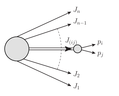
Figure 2.1: Factorisation of the real phase space for the $2\to 1$ clustering of partons $i,j$ into an off-shell Born and a two-particle phase space.

By utilising a factorisation of the real phase space corresponding to the clustering given in eq. (2.6), we obtain (cf. fig. 2.1)

$$d\Phi_{n+1}(P,\{p_{1},\ldots,p_{i},\ldots,p_{j},\ldots p_{n+1}\},\{m_{1},\ldots,m_{i},\ldots,m_{j},\ldots m_{n+1}\})$$ (2.12)

$$= d\Phi_{n}(P,\{J_{1},\ldots,\cancel{p_{i}},\;J_{(ij)},\ldots,\cancel{p_{j}},\ldots,J_{n}\},\{m_{1},\ldots,\cancel{m_{i}},\;M_{ij},\ldots,\cancel{m_{j}},\ldots,m_{n+1}\})$$

$$\times (2\pi)^{-1}d{M_{ij}}^{2}\;d\Phi_{2}(J_{(ij)},\{p_{i},p_{j}\},\{m_{i},m_{j}\})\;.$$

Using the parametrisation from the Born and virtual part for the $n$-particle phase space (with the off-shell momentum $J_{(ij)}$),

$${d\Phi_{n}(P,\{J_{1},\ldots,\cancel{p_{i}},\;J_{(ij)},\ldots,\cancel{p_{j}},\ldots,J_{n}\},\{m_{1},\ldots,\cancel{m_{i}},\;M_{ij},\ldots,\cancel{m_{j}},\ldots,m_{n+1}\})}$$

the same $(3n-2$) variables $\{x_{1},\ldots,x_{r}\}$ as in eq. (2.9) appear as independent variables. It is thus straightforward to integrate out the second delta-function

$$\delta^{(r)}\left(\vec{x}-\vec{x}(J^{(n+1)}_{1}\equiv J_{1},\ldots,J^{(n+1)}_{n}\equiv J_{n})\right)$$

in eq. (2) while the unresolved parton pair is to be integrated over the region ${\cal R}_{ij}$. The contribution of the real corrections to the differential cross section from the region ${\cal R}_{ij}$ reads

$${d^{r}\sigma^{\text{R}}_{{{\cal R}_{ij}}}\over d{x}_{1}\ldots d{x}_{r}} = {(2\pi)^{(3-3n)}\over 2^{n-1}}{1\over s}\;\int_{{{\cal R}_{ij}}}{d{M_{ij}}^{2}}\;{\cal J}(\vec{x})\;\left[\prod_{{k=1}}^{n}{1\over J^{0}_{k}}\right]\;d\Phi_{2}(J_{(ij)},\{p_{i},p_{j}\},\{m_{i},m_{j}\})$$ (2.13)

$$\times R\left(x_{a},x_{b};p_{1}(\vec{x},{M_{ij}},\phi_{i},\theta_{i}),\ldots,p_{n+1}(\vec{x},{M_{ij}},\phi_{i},\theta_{i})\right)\;.$$

The parametrisation of the $n+1$ partonic momenta $\{p_{1},\ldots,p_{n+1}\}$ in terms of $\{x_{1},\ldots,x_{r}\}$, ${M_{ij}}$ and the azimuthal and polar angle $\phi_{i}$ and $\theta_{i}$ of parton $i$ is fixed by the delta-functions in eq. (2.9) and the clustering of $n+1$ partonic momenta to $n$ jet momenta in the region ${\cal R}_{ij}$. The Jacobian ${\cal J}(\vec{x})$ occurring in eq. (2.13) is the same as in eq. (2.11).

Let us now investigate the contribution from regions ${\cal R}_{i}$ in which the parton $i$ is considered as part of the beam and needs to be integrated out. Since there is no recombination in this case, the momenta of the resolved jets are identified with the underlying partonic momenta.

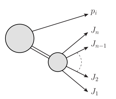
Figure 2.2: Real phase space for the unresolved parton $i$ as boosted Born and additional parton.

The real phase space $d\Phi_{n+1}$ can be factorised in terms of a boosted $n$-particle phase space and integrations over the degrees of freedom of the additional parton (cf. fig. 2.2). The momenta in the boosted $n$-particle phase space, corresponding to the $n$ resolved jets, can be parameterised by the same $(3n-2)$ variables as in eq. (2.9):

$$dx_{a}dx_{b}\;d\Phi_{n+1}(x_{a}P_{a}+x_{b}P_{b},\{p_{1},\ldots,p_{n+1}\},\{m_{1},\ldots,m_{n+1}\})$$

$$= {d^{4}p_{i}\over(2\pi)^{3}}\delta\left({p_{i}}^{2}-{m_{i}}^{2}\right)\;dx_{a}dx_{b}\;d\Phi_{n}(x_{a}P_{a}+x_{b}P_{b}-p_{i},\{J_{1},\ldots,J_{n}\},\{m_{1},\ldots,m_{n}\})$$

$$= {(2\pi)^{(4-3n)}\over 2^{n-1}}{1\over s}\;{\cal J}(\vec{x})\;dx_{1}\ldots dx_{r}\;{d^{3}p_{i}}$$

$$\times\;{(2\pi)^{-3}\over 2}\left[\prod_{k=1}^{n}d{J_{k}}^{2}\;\delta\left({J_{k}}^{2}-{m_{k}}^{2}\right)\;{1\over J_{k}^{0}}\right]\;{d{p_{i}}^{2}\over p_{i}^{0}}\;\delta\left({p_{i}}^{2}-{m_{i}}^{2}\right)\;d^{2}J^{\perp}_{1}\;\delta^{(2)}\left(-\vec{p}^{\perp}_{i}-\sum_{{k=1}}^{n}\vec{J}^{\perp}_{k}\right)$$

$$\times\;dx_{a}dx_{b}\;\delta\left(x_{a}-{p^{0}_{i}+p^{z}_{i}\over\sqrt{s}}-{1\over\sqrt{s}}\left(\sum_{k=1}^{n}(J^{0}_{k}+J^{z}_{k})\right)\right)\;\delta\left(x_{b}-{p^{0}_{i}-p^{z}_{i}\over\sqrt{s}}-{1\over\sqrt{s}}\left(\sum_{k=1}^{n}(J^{0}_{k}-J^{z}_{k})\right)\right)\;.$$

As in the previous case, the jet masses, the transverse momentum, and the $3$-momentum of the unresolved radiation appear as additional integration variables. On-shell conditions and momentum conservation again fix the former, while the $3$-momentum $\vec{p}_{i}$ and the variables $\{x_{1},\ldots,x_{r}\}$ are left as integration variables. It is thus straightforward to integrate out the second delta-function

$$\delta^{(r)}\left(\vec{x}-\vec{x}(J^{(n+1)}_{1}\equiv J_{1},\ldots,J^{(n+1)}_{n}\equiv J_{n})\right)$$

in eq. (2), leaving the unresolved radiation to be integrated over the region ${\cal R}_{i}$.

The contribution of the real corrections from the region ${\cal R}_{i}$ to the differential cross section is then given by

$${d^{r}\sigma^{\text{R}}_{{{\cal R}_{i}}}\over d{x}_{1}\ldots d{x}_{r}} = {(2\pi)^{(1-3n)}\over 2^{n}}{1\over s}\;\int_{{{\cal R}_{i}}}{d^{3}p_{i}\over p^{0}_{i}}\;{\cal J}(\vec{x})\;\left[\prod_{k=1}^{n}{1\over J_{k}^{0}}\right]\;R\left(x_{a},x_{b};p_{1}(\vec{x},\vec{p}_{i}),\ldots,p_{n+1}(\vec{x},\vec{p}_{i})\right)\;,$$

where the parametrisation of the $n+1$ partonic momenta $\{p_{1},\ldots,p_{n+1}\}$ in terms of $\{x_{1},\ldots,x_{r}\}$ and $\vec{p}_{i}$ is fixed by the delta-functions in eq. (2) and the identification of $n$ resolved parton momenta with $n$ jet momenta.

It is worth mentioning that with a slight modification of eq. (2) the contribution from the real corrections where the extra radiation $i$ is resolved as an additional jet with momentum $J_{i}$ but does not enter the event definition can be obtained: the integration over $\vec{J}_{i}$ has to be carried out over the region $\tilde{\cal R}_{i}$ of the real phase space where parton $i$ is resolved as an additional jet,

$${d^{r}\sigma^{\text{R}}_{\tilde{\cal R}_{i}}\over d{x}_{1}\ldots d{x}_{r}}=\int_{\tilde{\cal R}_{i}}{d^{3}J_{i}\over J^{0}_{i}}\;{\cal J}(\vec{x})\;\left[\prod_{k=1}^{n}{1\over J_{k}^{0}}\right]\;R\left(x_{a},x_{b};p_{1}(\vec{x},\vec{J}_{i}),\ldots,p_{n+1}(\vec{x},\vec{J}_{i})\right)\;.$$

Collecting the Born and virtual contributions (see eq. (2.11)) and the real corrections from the different regions ${\cal R}_{ij}$ (see eq. (2.13)), ${\cal R}_{i}$ (see eq. (2)), and $\tilde{\cal R}_{i}$ (see eq. (2)), we finally obtain the fully differential cross section including the NLO corrections (cf. eq. (2.8)). A validation of this approach for the example of single top-quark production is given in Appendix B.

3 Parton shower effects in fixed-order MEM analyses

In previous applications of the MEM at NLO to fully hadronic processes, the approach has been restricted by requiring a $3\to 2$ clustering in the jet algorithm [37, 38]. Therefore, only closure tests of the method, where the pseudodata have been generated with the modified clustering prescription, have been presented so far. The method presented in this paper and LABEL:Martini:2018imv extends the MEM at NLO to incorporate $2\to 1$ clusterings and therefore allows one to analyse realistic events.

We use the POWHEG-BOX [49, 50] to generate pseudodata. The events are subsequently showered using the Pythia8 parton-shower (PS) program [51]. During the parton-shower evolution, the top quark is kept stable, and corrections from hadronisation and underlying events have been neglected. Thus, the main difference between the pseudodata and the fixed-order NLO calculation used for the analysis is the inclusion of additional radiation in the events. This allows us for the first time to study the impact of parton-shower effects within the MEM at NLO accuracy.

For a concrete example, we study the top-quark mass determination from hadronic single top-quark production via the $t$-channel:

$$pp\rightarrow tj\;.$$ (3.1)

The event signature is given by a top-tagged jet $t$ in association with at least one light jet $j$. The sample is generated for the LHC at $\sqrt{s}=13$ TeV and a top-quark mass of $m_{t}=173.2$ GeV. The renormalisation and factorisation scales are set to $\mu_{R}=\mu_{F}=\mu_{0}=m_{t}$. Jets are defined using the $k_{t}$-algorithm [48] with a separation parameter of $R=0.4$. Unresolved partons are clustered by the $2\to 1$ recombination by summing their $4$-momenta. Resolved jets have to pass the following cuts on the transverse momentum and the pseudorapidity

$$p^{\perp}>p^{\perp}_{\text{min}}=30\text{ GeV},\qquad\quad|\eta|<\eta_{\text{max}}=3.5.$$

The detector is assumed to be blind outside these cuts. If there is more than one resolved light jet, the hardest one is used in the event definition. We assume that it is always possible to identify the jet containing the top quark. The resulting event sample for the fiducial phase space volume consists of $N=28031$ events.

The top-quark mass extraction proceeds as follows. For each showered POWHEG event $i$, the set of variables $({\eta_{t}}^{i},{E_{j}}^{i},{\eta_{j}}^{i},{\phi_{j}}^{i})$ is calculated from the top-tagged jet and the hardest light jet. The motivation for this choice of variables is two-fold. First of all, measuring angular variables is experimentally under better control than variables related to the energy of final-state objects. This is especially true for jets, since the jet-energy scale often represents a major uncertainty. By preferring the former over the latter, the deviations from trivial transfer functions should only be a moderate effect. Second, this set of variables is equivalent to the generic set given in eq. (2.10) with the respective variable transformation given in Appendix A. As long as the Jacobian is independent of the parameter to be estimated, the MEM and its results are invariant under any change of variables complying with the requirements of not fixing the jets’ masses and the overall transverse momentum given in section 2. However, it should be stressed that not all variables can be reached from the aforementioned ones by a variable transformation. This is not a restriction per se. It simply means that because of the intrinsic inclusiveness of the jets the contribution of the real corrections—the unresolved regions which need to be integrated out—depends on the chosen variables. For variables not reachable by a variable transformation, one can still use the procedure presented in this article. It would just mean that one has to start with a different set of variables.

For each event, the weight is calculated for a specific value of the top-quark mass (cf. eq. (2.8) and details in Appendix A). The corresponding likelihood function $\mathcal{L}(m_{t})$ is computed according to

$$\mathcal{L}(m_{t})=\prod_{i=1}^{N}\frac{1}{\sigma(m_{t})}\frac{d^{4}\sigma(m_{t})}{d{\eta_{t}}^{i}\;d{E_{j}}^{i}\;d{\eta_{j}}^{i}\;d{\phi_{j}}^{i}},$$ (3.2)

where only trivial transfer functions (i.e., delta-functions) have been used. For more details, we refer to LABEL:Martini:2018imv. Minimizing the negative log-likelihood function $(-\log\mathcal{L})$ with respect to the top-quark mass parameter yields the estimator for the top-quark mass $\widehat{m}_{t}$. We have checked that we correctly reproduce the input value if the pseudodata are generated using fixed-order predictions and parton-shower effects are neglected. Figure 3.1 shows the negative log-likelihood function for the POWHEG events as a function of the top-quark mass and for various scale choices at leading order (LO) and NLO in perturbation theory. The leading-order results are shown in blue for three different scales, the central scale $\mu_{0}$ (blue) and scale variations $\mu_{0}/2$ (light blue) as well as $2\mu_{0}$ (dark blue). The red curves are obtained by including the NLO QCD corrections in the definition of the likelihood functions and are also shown for three different scales: $\mu_{0}$ (red), $\mu_{0}/2$ (light red), and $2\mu_{0}$ (dark red). The vertical green line denotes the value for the top-quark mass used for the generation of the pseudodata. The minimum of the curves yields the estimator for the top-quark mass $\widehat{m}_{t}$ and the width of the parabola gives the statistical uncertainty $\Delta\widehat{m}_{t}$ on the estimator. The estimated top-quark mass using the Born approximation for the central scale is thus given by $\widehat{m}_{t}=(150.19\pm 1.38_{\text{stat}})$ GeV. Based on the results for the two other scale settings, the uncertainty due to neglected higher-order corrections is estimated to be of the order of $\pm 5$ GeV. We observe a significant difference between the results obtained from the MEM using LO matrix elements and the input value. In particular, the observed shift of about 22 GeV is not covered by the uncertainties. Using the MEM based on leading-order matrix elements thus requires a significant calibration to reproduce the input value.

Using, on the other hand, the full NLO QCD calculation for the determination of the event weights entering the likelihood function, the estimator for the top-quark mass gives $\widehat{m}^{\textrm{NLO}}_{t}=(163.75\pm 1.83_{\text{stat}})$ GeV. A significant reduction of the scale uncertainty is observed. The uncertainty goes down from the aforementioned $\pm 5$ GeV to $+1$ GeV and $-3$ GeV at NLO. Furthermore the shift compared to the input value is reduced to 10 GeV compared to 22 GeV at leading order.

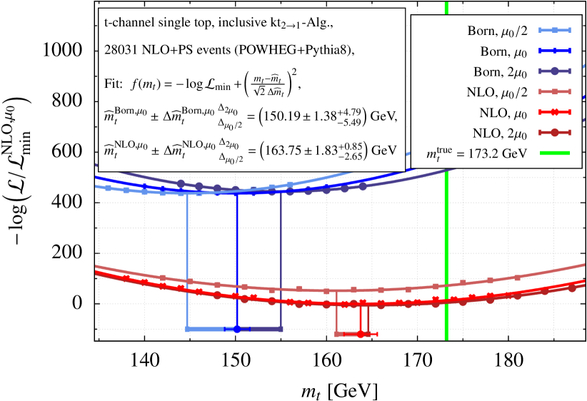
Figure 3.1: Top-quark mass extraction with the Matrix Element Method from $t$-channel single top-quark events at the LHC generated with POWHEG and Pythia8.

In fact, a shift in the extracted top-quark mass to lower mass values is expected due to parton-shower effects in the pseudodata which are not taken into account in the MEM: multiple parton emissions lead to a modification of the phase space density, which results in shape differences in differential distributions compared to fixed-order NLO computations. The MEM is very sensitive to small distortions of the differential distributions. As the parton-shower tends to soften the $p_{\perp}$ distribution, the MEM favours a smaller mass value.

Note that the analysis based on the likelihood function given in eq. (3.2) is only sensitive to the normalised multidifferential cross section. As argued in LABEL:Martini:2017ydu,Martini:2018imv, the information about the fiducial cross section can improve the parameter determination. To incorporate the information on the total number of events in the sample, the extended likelihood function, defined by

$$\mathcal{L}_{\text{ext}}(m_{t})={{\nu(m_{t})^{N}}\over{N!}}e^{-\nu(m_{t})}\mathcal{L}(m_{t})=\frac{L^{N}}{N!}e^{-\sigma(m_{t})L}\prod_{i=1}^{N}\frac{d^{4}\sigma(m_{t})}{d{\eta_{t}}^{i}\;d{E_{j}}^{i}\;d{\eta_{j}}^{i}\;d{\phi_{j}}^{i}},$$ (3.3)

is used. Here, $\nu(m_{t})=L\cdot\sigma(m_{t})$ is the predicted number of events, where $L$ denotes the integrated luminosity of the experiment. For the pseudodata used in the analysis, the integrated luminosity is given by $N=L\cdot\sigma^{\textrm{NLO+PS}}$, where $\sigma^{\textrm{NLO+PS}}$ is the fiducial cross section corresponding to the simulated data. Including the information on the number of recorded events should give a significant improvement: while the parton shower tends to soften the $p_{\perp}$ distribution leading to the aforementioned smaller mass values, the total number of events is only mildly affected through acceptance effects. Since a smaller mass value leads to larger cross sections and thus a larger number of events, including this information through the extended likelihood increases the sensitivity of the analysis. The results of the extended likelihood analysis are shown in Fig. 3.2.

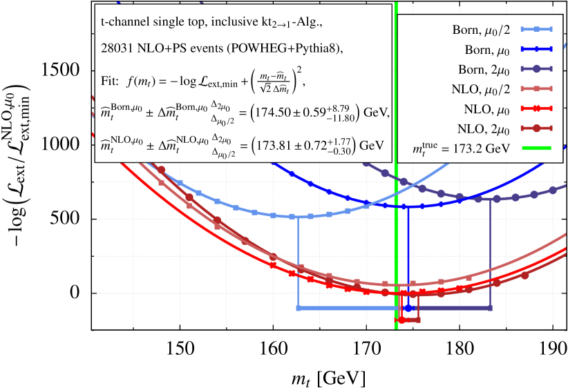
Figure 3.2: Top-quark mass extraction with the Extended Matrix Element Method from $t$-channel single top-quark events at the LHC generated with POWHEG and Pythia8.

The fit improves significantly compared to the previous analysis. At LO and NLO accuracy, the estimated mass value is now compatible with the input value. Including the information about the normalisation, the Born approximation yields a top-quark mass estimator of $\widehat{m}_{t}=174.50$ GeV with a statistical uncertainty of $\Delta\widehat{m}_{t}=\pm 0.59$ GeV. While the statistical uncertainty is reduced by more than a factor of $2$, the systematic uncertainty due to scale variations is enlarged by more than a factor of $2$, which amounts to roughly $\pm 10$ GeV. Repeating the extraction including the NLO QCD corrections in the extended likelihood function improves the analysis significantly with respect to the Born approximation. The top-quark mass estimator and its statistical uncertainty are given by $\widehat{m}^{\textrm{NLO}}_{t}=(173.81\pm 0.72_{\text{stat}})$ GeV, which is compatible with the input mass within one standard deviation. Also, in the case of the extended likelihood function at NLO accuracy, the statistical uncertainty is reduced by more than a factor of $2$. In contrast to the Born approximation, the systematic uncertainty, as obtained by scale variations, is also reduced at NLO and amounts to an uncertainty of $-0.3$ GeV and $+1.8$ GeV. Furthermore, in the extended likelihood approach, the NLO estimator is covered by the uncertainty of the leading-order estimator, which justifies the use of scale variations as an estimate for the missing higher-order corrections. As mentioned above, the parton shower does not have a significant impact on the number of accepted events in comparison to the fixed-order NLO calculation. However, the predicted number of events depends approximately linearly on the value of top-quark mass parameter [38, 52]. Therefore, the extended likelihood analysis is driven towards top-quark mass values, which correspond to a compatible prediction of the number of events with the pseudodata. It is worth noting that with roughly $30000$ events the uncertainty on the extracted top-quark mass is already dominated by systematic uncertainties. In the above analysis, no uncertainty for the luminosity is included. To estimate the impact of this additional uncertainty, we assume a relative uncertainty $\Delta L/L\approx 2\%$ [53]. Repeating the extended likelihood analysis while varying the value of $L$ by $\pm 2\%$ results in additional shifts in both the LO and the NLO estimators for the top-quark mass of about $\pm 2$ GeV. Although, the inclusive cross section provides important information within the MEM—pushing the extracted mass to the value used in the simulation—we stress that the inclusive cross section alone would lead to much larger uncertainties.

4 Conclusion

In this article, an algorithm to calculate fully differential event weights including NLO QCD corrections is presented. The weight is calculated for events containing jets and not partons. We emphasise that the weight is calculated a posteriori for a given jet event. This is a significant extension to existing approaches used in MC tools which allow the generation of jet events together with the corresponding weight but do not allow one to evaluate the weight for a given jet event. In contrast to previous work [37, 38], the conventional $2\to 1$ recombination is used—no change of the recombination procedure is required. The approach is thus directly applicable in the experimental analysis. The method relies on properly chosen variables to describe the jet event. As explained in detail in the article, the variables must not depend on the jet masses since this would spoil the pointwise one-to-one correspondence of real and virtual corrections. We give a concrete example for a consistent choice of variables together with the required formulas and show how the phase space is rewritten to allow the evaluation of the fully differential event weight. The approach is completely general and can be applied to other LHC processes.

The method has been used to study for the first time parton-shower effects in the MEM@NLO. We illustrated the impact of the parton shower exemplarily within the context of parameter determination. We studied the top-quark mass extraction with the Matrix Element Method with likelihood functions that include the fully NLO QCD corrected event weight. Pseudodata are generated using the POWHEG-BOX with subsequent showering using Pythia8 to incorporate parton-shower effects. We observe that a significant calibration would be required to reconstruct the input value from the value extracted by the MEM. This is not surprising since the parton shower leads to a significant distortion of the distributions preferring smaller mass values. Within the extended likelihood approach, however, perfect agreement with the input value for the top-quark mass of the pseudodata is found. In particular, we show that in this approach no calibration is required and observe a substantial reduction of the systematic uncertainties when NLO corrections are taken into account in the calculation of the likelihood. We expect that these findings are not specific to the example studied here but apply also to other processes.

Actually, the approach is not restricted to a specific process. The ability to predict event weights at NLO accuracy for jet events enables the application of the Matrix Element Method at NLO for events recorded by the experiments without a modification of the recombination procedure in conventional jet algorithms.

Finally, in refs. [54, 55, 56, 57], information from both the leading-order matrix element as well as the parton shower is taken into account when calculating the likelihood. It is conceivable that combining that approach with the method presented in this work will prove beneficial en route to an unbiased Matrix Element Method for collider experiments.

In this article, the transfer functions are modelled as delta-functions. Although the impact of transfer functions might be reduced because of the better jet modelling in NLO, it is clear that a fully realistic analysis should also include transfer functions as extracted in the experiments.

Appendix A Calculational details

In this Appendix, we provide necessary details for the implementation of the fully differential NLO weights used in this publication.

We start the discussion with the Born phase space. Due to momentum conservation and on-shell conditions, each event is fully described by four variables $x_{1},\ldots,x_{4}$. The pseudorapidity of the top-tagged jet and the energy, the pseudorapidity and the azimuthal angle of the (hardest) light jet are chosen. Each set of measured values $\vec{x}=(\eta_{t},E_{j},\eta_{j},\phi_{j})$ specifies the $4$-momenta of the resolved jets as functions of the squared jet masses ${J_{j}}^{2}$ and ${J_{t}}^{2}$,

$$J_{t} = \left(E_{t},\;-J^{\perp}\cos{\phi_{j}},\;-J^{\perp}\sin{\phi_{j}},\;J^{\perp}\sinh{\eta_{t}}\right),$$

$$J_{j} = \left(E_{j},\;J^{\perp}\cos{\phi_{j}},\;J^{\perp}\sin{\phi_{j}},\;J^{\perp}\sinh{\eta_{j}}\right)$$ (A.1)

with

$$J^{\perp}=J^{\perp}_{t}=J^{\perp}_{j}={\sqrt{{E_{j}}^{2}-{J_{j}}^{2}}\over\cosh{\eta_{j}}},\quad E_{t}=\sqrt{{J^{\perp}}^{2}\cosh^{2}{\eta_{t}}+{J_{t}}^{2}}$$

and the Jacobian

$${\cal J}(\eta_{t},E_{j},\eta_{j},\phi_{j})=\left|\partial(J^{z}_{t},J^{x}_{j},J^{y}_{j},J^{z}_{j})\over\partial(\eta_{t},E_{j},\eta_{j},\phi_{j})\right|={E_{j}\;{J^{\perp}_{t}}{J^{\perp}_{j}}\cosh{\eta_{t}}\over\cosh{\eta_{j}}}.$$ (A.2)

From eq. (2.11), the Born and virtual contribution of the NLO event weight follows as

$${d^{4}\sigma^{\text{BV}}\over d{\eta_{t}}\;d{E_{j}}\;d{\eta_{j}}\;d{\phi_{j}}}=(2\pi)^{-2}{{J^{\perp}}^{2}\cosh{\eta_{t}}\over 2\;s\;E_{t}\;\cosh{\eta_{j}}}\;\left[B+V\right](x_{a},x_{b};J_{t},J_{j})$$ (A.3)

with the jet momenta from eq. (A). According to eq. (2.9), the squared jet masses are given by ${J_{t}}^{2}={m_{t}}^{2}$ and ${J_{j}}^{2}=0$, and the momentum fractions follow as

$$x_{a} = {1\over\sqrt{s}}\left(E_{t}+E_{j}+J^{\perp}(\sinh\eta_{t}+\sinh\eta_{j})\right),$$

$$x_{b} = {1\over\sqrt{s}}\left(E_{t}+E_{j}-J^{\perp}(\sinh\eta_{t}+\sinh\eta_{j})\right).$$ (A.4)

In the real corrections, the top quark with momentum $p_{t}$ and a light parton with momentum $p_{l}$ are produced together with additional radiation with momentum $p_{r}$:

$$p_{a}+p_{b}\rightarrow p_{t}+p_{l}+p_{r}\;.$$ (A.5)

The phase space of the real corrections contributing to single top-quark production in association with a light jet can thus be split into the regions ${\cal R}_{tr}$, ${\cal R}_{lr}$, ${\cal R}_{r}$, and $\tilde{\cal R}_{r}$. For the clustering of the extra radiation with the top quark, eq. (2.13) yields

$${d^{4}\sigma^{\text{R}}_{{{\cal R}_{tr}}}\over d{\eta_{t}}\;d{E_{j}}\;d{\eta_{j}}\;d{\phi_{j}}} = (2\pi)^{-3}\frac{{J^{\perp}}^{2}\cosh{\eta_{t}}}{2s\;\cosh{\eta_{j}}}\;\int_{{{\cal R}_{tr}}}{d{J_{t}}^{2}\over E_{t}}\;d\Phi_{2}(J_{t},\{p_{t},p_{r}\},\{m_{t},0\})\;$$ (A.6)

$$\quad\times\left(R(x_{a},x_{b};p_{t},J_{j},p_{r})+R(x_{a},x_{b};p_{t},p_{r},J_{j})\right)$$

with the jet momenta parametrisation from eq. (A). Because of the on-shell conditions, the squared jet masses follow as ${J_{t}}^{2}={M_{tr}}^{2}=(p_{t}+p_{r})^{2}$ and ${J_{j}}^{2}=0$. The parton momentum fractions are again given by eq. (A). Note that eq. (A.6) already takes into account that either of the massless quarks can be clustered together with the top quark, while the other one constitutes the light jet.

In the case where the light jet is obtained from the clustering of the light quark and the additional radiation, eq. (2.13) yields

$${d^{4}\sigma^{\text{R}}_{{{\cal R}_{lr}}}\over d{\eta_{t}}\;d{E_{j}}\;d{\eta_{j}}\;d{\phi_{j}}} = (2\pi)^{-3}\frac{\cosh{\eta_{t}}}{2s\;\cosh{\eta_{j}}}\;\int_{{{\cal R}_{lr}}}{d{J_{j}}^{2}}\;{{J^{\perp}}^{2}\over E_{t}}\;d\Phi_{2}(J_{j},\{p_{l},p_{r}\},\{0,0\})\;R(x_{a},x_{b};J_{t},p_{l},p_{r})$$

with the jet momenta from eq. (A). The on-shell conditions result in ${J_{t}}^{2}={m_{t}}^{2}$ and ${J_{j}}^{2}={M_{lr}}^{2}=(p_{l}+p_{r})^{2}$, while the parton momentum fractions are again given by eq. (A).

In the regions of the phase space where the extra radiation is associated with the beam, the jet momenta have to be parametrised by the variables $(\eta_{t},E_{j},\eta_{j},\phi_{j})$ and the $3$-momentum of the extra radiation in order to ensure momentum conservation,

$$J_{t} = \left(E_{t},\;-J^{\perp}_{t}\cos{\phi_{t}},\;-J^{\perp}_{t}\sin{\phi_{t}},\;J^{\perp}_{t}\sinh{\eta_{t}}\right)\;,$$

$$J_{j} = \left(E_{j},\;J^{\perp}_{j}\cos{\phi_{j}},\;J^{\perp}_{j}\sin{\phi_{j}},\;J^{\perp}_{j}\sinh{\eta_{j}}\right)$$ (A.8)

with

$$J^{\perp}_{j}=\displaystyle{E_{j}\over\cosh{\eta_{j}}}\;,\quad J^{\perp}_{t}=\sqrt{\left(J^{\perp}_{j}\cos{\phi_{j}}+p^{x}_{r}\right)^{2}+\left(J^{\perp}_{j}\sin{\phi_{j}}+p^{y}_{r}\right)^{2}}\;,$$

$$\tan\phi_{t}=\displaystyle{J^{\perp}_{j}\sin{\phi_{j}}+p^{y}_{r}\over J^{\perp}_{j}\cos{\phi_{j}}+p^{x}_{r}}\;,\quad E_{t}=\sqrt{{J^{\perp}_{t}}^{2}\cosh^{2}{\eta_{t}}+m^{2}_{t}}\;.$$

Note that the jet momenta defined in eq. (A) fulfill the on-shell conditions in eq. (2) by construction: ${J_{t}}^{2}={m_{t}}^{2}$ and ${J_{j}}^{2}=0$. Using this parametrisation and eq. (2) together with eq. (A.2) yields

$${d^{4}\sigma^{\text{R}}_{{{\cal R}_{r}}}\over d{\eta_{t}}\;d{E_{j}}\;d{\eta_{j}}\;d{\phi_{j}}} = (2\pi)^{-5}{{J^{\perp}_{j}}\cosh{\eta_{t}}\over 4s\;\cosh{\eta_{j}}}\;\int_{{{\cal R}_{r}}}{d^{3}p_{r}}\;{{J^{\perp}_{t}}\over E_{t}\;|\vec{p}_{r}|}$$ (A.9)

$$\quad\times\left(R(x_{a},x_{b};J_{t},J_{j},p_{r})+R(x_{a},x_{b};J_{t},p_{r},J_{j})\right)$$

with the parton momentum fractions given by

$$x_{a} = {1\over\sqrt{s}}\left(E_{t}+E_{j}+|\vec{p}_{r}|+J^{\perp}_{t}\sinh\eta_{t}+J^{\perp}_{j}\sinh\eta_{j}+p^{z}_{r}\right)\;,$$

$$x_{b} = {1\over\sqrt{s}}\left(E_{t}+E_{j}+|\vec{p}_{r}|-J^{\perp}_{t}\sinh\eta_{t}-J^{\perp}_{j}\sinh\eta_{j}-p^{z}_{r}\right)\;.$$ (A.10)

Again, either of the massless quarks can escape detection, while the other one constitutes the light jet.

The region $\tilde{\cal R}_{r}$, corresponding to the extra radiation being resolved as an additional but softer light jet, contributes to the event weight as (cf. eq. (2))

$${d^{4}\sigma^{\text{R}}_{{\tilde{\cal R}_{r}}}\over d{\eta_{t}}\;d{E_{j}}\;d{\eta_{j}}\;d{\phi_{j}}} = (2\pi)^{-5}{{J^{\perp}_{j}}\cosh{\eta_{t}}\over 4s\;\cosh{\eta_{j}}}\;\int_{{\tilde{\cal R}_{r}}}{d^{3}J_{r}}\;{{J^{\perp}_{t}}\over E_{t}\;|\vec{J}_{r}|}\;\Theta\left(J^{\perp}_{j}-J^{\perp}_{r}\right)$$ (A.11)

$$\quad\times\left(R(x_{a},x_{b};J_{t},J_{j},J_{r})+R(x_{a},x_{b};J_{t},J_{r},J_{j})\right)$$

with the parametrisation of the jet momenta and parton momentum fractions given in eq. (A) and eq. (A) with $p_{r}\rightarrow J_{r}$. According to eq. (2.8), the weight including NLO corrections for a jet event $t,j$ defined by $\eta_{t}$, $E_{j}$, $\eta_{j}$, and $\phi_{j}$ is given by the sum of the Born and virtual contribution (see eq. (A.3)) and the real corrections from the regions ${\cal R}_{tr}$ (see eq. (A.6)), ${\cal R}_{lr}$ (see eq. (A)), ${\cal R}_{r}$ (see eq. (A.9)), and $\tilde{\cal R}_{r}$ (see eq. (A.11)). We stress that a $2\to 1$ recombination is used where the momentum of the resulting jet is defined as the $4$-momentum sum of the recombined partons.

Appendix B Validation

In this Appendix, we show a short validation of the presented method. To this end, we generated approximately $40000$ unweighted events at NLO accuracy to compute differential distributions, which are compared to an ordinary Monte-Carlo integration. The input parameters for the simulation are the same as described in section 3, which for brevity we do not repeat here.

The red dashed histograms in fig. B.1 show the $E_{j}$, $n_{j}$, and $\eta_{t}$ distributions obtained from the unweighted NLO event sample. These distributions are compared with the results of independent calculations using a parton level Monte-Carlo integration (blue solid histogram in fig. B.1). In the lower part of the plots, the respective pull distributions, p-values, and reduced $\chi^{2}$ of the comparison of the two histograms as described in LABEL:Gagunashvili:2007zz and implemented in refs. [59, 60, 61] are given. The results in fig. B.1 show that the unweighted events are indeed distributed according to the cross section calculated at NLO accuracy. Within the statistical uncertainties, the results from the parton-level Monte Carlo are in perfect agreement with the results obtained from the sample of unweighted events.

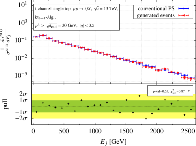
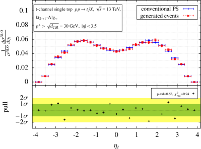
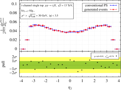
Figure B.1: Energy and pseudorapidity distributions for $t$-channel single top-quark production calculated at NLO accuracy using a conventional parton-level Monte Carlo with $2\to 1$ jet clustering (solid blue) compared to histograms filled with generated NLO events (dashed red). At the bottom of the plots, the pull distributions together with the p-value and the reduced $\chi^{2}$ of the histogram comparisons are shown.

References

- [1] P. Nason, Theoretical Progress in QCD, Nucl. Part. Phys. Proc. 273-275 (2016) 72–81.
- [2] F. Caola, NNLO corrections for LHC processes, in Proceedings, 50th Rencontres de Moriond, QCD and high energy interactions: La Thuile, Italy, March 21-28, ,ISBN 978-2-9546400-7-5. - [S.l.] : ARISF, 2015. - S. 259-262 [online].
- [3] G. Heinrich, QCD calculations for the LHC: status and prospects, in 5th Large Hadron Collider Physics Conference (LHCP 2017) Shanghai, China, May 15-20, 2017, 2017. [arXiv:1710.04998].
- [4] C. Duhr, QCD at NNLO and beyond, Nucl. Part. Phys. Proc. 273-275 (2016) 2128–2135.
- [5] S. Badger, B. Biedermann, P. Uwer, and V. Yundin, Numerical evaluation of virtual corrections to multi-jet production in massless QCD, Comput. Phys. Commun. 184 (2013) 1981–1998, [arXiv:1209.0100].
- [6] G. Bevilacqua, M. Czakon, M. V. Garzelli, A. van Hameren, A. Kardos, C. G. Papadopoulos, R. Pittau, and M. Worek, HELAC-NLO, Comput. Phys. Commun. 184 (2013) 986–997, [arXiv:1110.1499].
- [7] G. Cullen et al., GS-2.0: a tool for automated one-loop calculations within the Standard Model and beyond, Eur. Phys. J. C74 (2014), no. 8 3001, [arXiv:1404.7096].
- [8] J. Alwall, R. Frederix, S. Frixione, V. Hirschi, F. Maltoni, O. Mattelaer, H. S. Shao, T. Stelzer, P. Torrielli, and M. Zaro, The automated computation of tree-level and next-to-leading order differential cross sections, and their matching to parton shower simulations, JHEP 07 (2014) 079, [arXiv:1405.0301].
- [9] S. Frixione, P. Nason, and C. Oleari, Matching NLO QCD computations with Parton Shower simulations: the POWHEG method, JHEP 11 (2007) 070, [arXiv:0709.2092].
- [10] T. Gleisberg, S. Hoeche, F. Krauss, M. Schonherr, S. Schumann, F. Siegert, and J. Winter, Event generation with SHERPA 1.1, JHEP 02 (2009) 007, [arXiv:0811.4622].
- [11] J. M. Campbell and R. K. Ellis, MCFM for the Tevatron and the LHC, Nucl. Phys. Proc. Suppl. 205-206 (2010) 10–15, [arXiv:1007.3492].
- [12] M. Czakon, P. Fiedler, D. Heymes, and A. Mitov, NNLO QCD predictions for fully-differential top-quark pair production at the Tevatron, JHEP 05 (2016) 034, [arXiv:1601.05375].
- [13] R. Boughezal, F. Caola, K. Melnikov, F. Petriello, and M. Schulze, Higgs boson production in association with a jet at next-to-next-to-leading order in perturbative QCD, JHEP 06 (2013) 072, [arXiv:1302.6216].
- [14] R. Boughezal, J. M. Campbell, R. K. Ellis, W. Focke, C.and Giele, X. Liu, F. Petriello, and C. Williams, Color singlet production at NNLO in MCFM, Eur. Phys. J. C77 (2017), no. 1 7, [arXiv:1605.08011].
- [15] S. Catani, S. Devoto, M. Grazzini, S. Kallweit, J. Mazzitelli and H. Sargsyan, Top-quark pair hadroproduction at next-to-next-to-leading order in QCD, Phys. Rev. D 99, no. 5, 051501 (2019) [arXiv:1901.04005].
- [16] R. Bonciani, G. Degrassi, P. P. Giardino and R. Gröber, Analytical Method for Next-to-Leading-Order QCD Corrections to Double-Higgs Production, Phys. Rev. Lett. 121, no. 16, 162003 (2018) [arXiv:1806.11564].
- [17] X. Chen, T. Gehrmann, N. Glover, M. Höfer and A. Huss, Isolated photon and photon+jet production at NNLO QCD accuracy, [arXiv:1904.01044].
- [18] J. Cruz-Martinez, T. Gehrmann, E. W. N. Glover and A. Huss, Second-order QCD effects in Higgs boson production through vector boson fusion, Phys. Lett. B 781, 672 (2018) [arXiv:1802.02445].
- [19] J. Currie, A. Gehrmann-De Ridder, T. Gehrmann, E. W. N. Glover, A. Huss and J. Pires, Precise predictions for dijet production at the LHC, Phys. Rev. Lett. 119, no. 15, 152001 (2017) [arXiv:1705.10271].
- [20] A. Gehrmann-De Ridder, T. Gehrmann, E. W. N. Glover, A. Huss and T. A. Morgan, The NNLO QCD corrections to Z boson production at large transverse momentum, JHEP 1607, 133 (2016) [arXiv:1605.04295].
- [21] T. Gehrmann, M. Grazzini, S. Kallweit, P. Maierhöfer, A. von Manteuffel, S. Pozzorini, D. Rathlev and L. Tancredi, Production at Hadron Colliders in Next to Next to Leading Order QCD, Phys. Rev. Lett. 113, no. 21, 212001 (2014) [arXiv:1408.5243].
- [22] S. Abreu, J. Dormans, F. Febres Cordero, H. Ita, B. Page and V. Sotnikov, Analytic Form of the Planar Two-Loop Five-Parton Scattering Amplitudes in QCD, JHEP 1905, 084 (2019) [arXiv:1904.00945].
- [23] S. Badger, C. Brønnum-Hansen, H. B. Hartanto and T. Peraro, First look at two-loop five-gluon scattering in QCD, Phys. Rev. Lett. 120, no. 9, 092001 (2018) [arXiv:1712.02229].
- [24] H. B. Hartanto, S. Badger, C. Brønnum-Hansen and T. Peraro, A numerical evaluation of planar two-loop helicity amplitudes for a W-boson plus four partons, [arXiv:1906.11862].
- [25] S. Abreu, J. Dormans, F. Febres Cordero, H. Ita and B. Page, Analytic Form of Planar Two-Loop Five-Gluon Scattering Amplitudes in QCD, Phys. Rev. Lett. 122, no. 8, 082002 (2019) [arXiv:1812.04586].
- [26] M. Grazzini, G. Heinrich, S. Jones, S. Kallweit, M. Kerner, J. M. Lindert and J. Mazzitelli, Higgs boson pair production at NNLO with top quark mass effects, JHEP 1805, 059 (2018) [arXiv:1803.02463].
- [27] M. Brucherseifer, F. Caola and K. Melnikov, On the NNLO QCD corrections to single-top production at the LHC, Phys. Lett. B 736, 58 (2014) [arXiv:1404.7116].
- [28] F. Caola, G. Luisoni, K. Melnikov and R. Röntsch, NNLO QCD corrections to associated production and decay, Phys. Rev. D 97, no. 7, 074022 (2018) [arXiv:1712.06954].
- [29] C. Anastasiou, C. Duhr, F. Dulat, F. Herzog, and B. Mistlberger, Higgs Boson Gluon-Fusion Production in QCD at Three Loops, Phys. Rev. Lett. 114 (2015) 212001, [arXiv:1503.06056].
- [30] B. Mistlberger, Higgs boson production at hadron colliders at N3LO in QCD, JHEP 05 (2018) 028, [arXiv:1802.00833].
- [31] J. Currie, T. Gehrmann, E. W. N. Glover, A. Huss, J. Niehues, and A. Vogt, N3LO corrections to jet production in deep inelastic scattering using the Projection-to-Born method, JHEP 05 (2018) 209, [arXiv:1803.09973].
- [32] F. Herzog, B. Ruijl, T. Ueda, J. A. M. Vermaseren, and A. Vogt, On Higgs decays to hadrons and the R-ratio at N4LO, JHEP 08 (2017) 113, [arXiv:1707.01044].
- [33] J. Brehmer, K. Cranmer, I. Espejo, F. Kling, G. Louppe and J. Pavez, Effective LHC measurements with matrix elements and machine learning, [arXiv:1906.01578]
- [34] J. R. Andersen et al., Les Houches 2017: Physics at TeV Colliders Standard Model Working Group Report, arXiv:1803.07977 [hep-ph], [arXiv:1803.07977].
- [35] J. Alwall, A. Freitas, and O. Mattelaer, The Matrix Element Method and QCD Radiation, Phys. Rev. D83 (2011) 074010, [arXiv:1010.2263].
- [36] J. M. Campbell, W. T. Giele, and C. Williams, The Matrix Element Method at Next-to-Leading Order, JHEP 11 (2012) 043, [arXiv:1204.4424].
- [37] T. Martini and P. Uwer, Extending the Matrix Element Method beyond the Born approximation: Calculating event weights at next-to-leading order accuracy, JHEP 09 (2015) 083, [arXiv:1506.08798].
- [38] T. Martini and P. Uwer, The Matrix Element Method at next-to-leading order QCD for hadronic collisions: Single top-quark production at the LHC as an example application, [arXiv:1712.04527].
- [39] ATLAS Collaboration, G. Aad et al., Evidence for single top-quark production in the -channel in proton-proton collisions at 8 TeV with the ATLAS detector using the Matrix Element Method, Phys. Lett. B756 (2016) 228–246, [arXiv:1511.05980].
- [40] T. M. Figy and W. T. Giele, A Forward Branching Phase Space Generator for Hadron colliders, [arXiv:1806.09678].
- [41] T. Martini, The Matrix Element Method at next-to-leading order QCD using the example of single top-quark production at the LHC. PhD thesis, Humboldt U., Berlin, 2018-06-26. [arXiv:1807.06859].
- [42] R. Baumeister and S. Weinzierl, Matrix element method at next-to-leading order for arbitrary jet algorithms, Phys. Rev. D95 (2017), no. 3 036019, [arXiv:1612.07252].
- [43] W. T. Giele, Improved Partonic Event Generators at Lepton Colliders, [arXiv:1504.02137].
- [44] S. Weinzierl, A General algorithm to generate unweighted events for next-to-leading order calculations in electron positron annihilation, JHEP 08 (2001) 028, [hep-ph/0106146].
- [45] S. Weinzierl and D. A. Kosower, QCD corrections to four jet production and three jet structure in e+ e- annihilation, Phys. Rev. D60 (1999) 054028, [hep-ph/9901277].
- [46] Z. Nagy, Next-to-leading order calculation of three jet observables in hadron hadron collision, Phys. Rev. D68 (2003) 094002, [hep-ph/0307268].
- [47] S. Alekhin, S. Moch and S. Thier, Determination of the top-quark mass from hadro-production of single top-quarks, Phys. Lett. B763 (2016) 341, [arXiv:1608.05212].
- [48] M. Cacciari, G. P. Salam, and G. Soyez, FastJet User Manual, Eur. Phys. J. C72 (2012) 1896, [arXiv:1111.6097].
- [49] S. Alioli, P. Nason, C. Oleari and E. Re, NLO single-top production matched with shower in POWHEG: s- and t-channel contributions, JHEP 0909 (2009) 111 Erratum: [JHEP 1002 (2010) 011] [arXiv:0907.4076].
- [50] S. Alioli, P. Nason, C. Oleari and E. Re, A general framework for implementing NLO calculations in shower Monte Carlo programs: the POWHEG BOX, JHEP 06 (2010) 043 [arXiv:1002.2581].
- [51] T. Sjöstrand et al., An Introduction to PYTHIA 8.2, Comput. Phys. Commun. 191, 159 (2015) [arXiv:1410.3012].
- [52] P. Kant, O. M. Kind, T. Kintscher, T. Lohse, T. Martini, S. Mölbitz, P. Rieck and P. Uwer, HatHor for single top-quark production: Updated predictions and uncertainty estimates for single top-quark production in hadronic collisions, Comput. Phys. Commun. 191, 74 (2015) [arXiv:1406.4403].
- [53] ATLAS Collaboration, M. Aaboud et al., Luminosity determination in pp collisions at = 8 TeV using the ATLAS detector at the LHC, Eur. Phys. J. C76 (2016), no. 12 653, [arXiv:1608.03953].
- [54] D. E. Soper and M. Spannowsky, Finding physics signals with shower deconstruction, Phys.Rev. D84 (2011) 074002, [arXiv:1102.3480].
- [55] D. E. Soper and M. Spannowsky, Finding top quarks with shower deconstruction, Phys.Rev. D87 (2013) 054012, [arXiv:1211.3140].
- [56] D. E. Soper and M. Spannowsky, Finding physics signals with event deconstruction, Phys. Rev. D89 (2014), no. 9 094005, [arXiv:1402.1189].
- [57] S. Prestel and M. Spannowsky, HYTREES: Combining Matrix Elements and Parton Shower for Hypothesis Testing, Eur. J Phys. C 79, 546 (2019), [arXiv:1901.11035].
- [58] N. D. Gagunashvili, Pearson’s chi-square test modifications for comparison of unweighted and weighted histograms and two weighted histograms, PoS ACAT (2007) 060.
- [59] R. Brun and F. Rademakers, ROOT: An object oriented data analysis framework, Nucl. Instrum. Meth. A389 (1997) 81–86.
- [60] I. Antcheva et al., ROOT: A C++ framework for petabyte data storage, statistical analysis and visualization, Comput. Phys. Commun. 180 (2009) 2499–2512, [arXiv:1508.07749].
- [61] L. Moneta, I. Antcheva, and R. Brun, Recent developments of the ROOT mathematical and statistical software, J. Phys. Conf. Ser. 119 (2008) 042023.