Ultra-high differential mobility and velocity of Néel walls in spin valves with planar-transverse polarizers under low perpendicularly injected currents

Abstract

Transverse domain wall (TDW) dynamics in long and narrow spin valves with perpendicular current injection is theoretically investigated. We demonstrate that stable traveling-wave motion of TDWs with finite velocity survives for strong enough planar-transverse polarizers. For typical ferromagnetic materials (for example, Co) and achievable spin polarization ($P=0.6$), TDWs acquire a velocity of $10^{3}$ m/s under a current density below $10^{7}$ $\mathrm{A/cm^{2}}$. This efficiency is comparable with that of perpendicular polarizers. More importantly, in this case the wall has ultra-high “differential mobility” around the onset of stable wall excitation. Our results open new possibilities for developing magnetic nanodevices based on TDW propagation with low energy consumption. Also, analytics for parallel and perpendicular polarizers perfectly explains existing simulation findings. Finally, further boosting of TDWs by external uniform transverse magnetic fields is investigated and turns out to be efficient.

I I. Introduction

Tremendous progress in fabrication technology of non-volatile magnetic nanodevices has led to a great revolution in modern information industryLeeuw_RPP_1980 ; Bauer_RMP_2005 ; Klaui_JPCM_2008 . In these nanodevices, magnetic domains with different orientations build zeros and ones in binary world. Intermediate regions separating these domains are the domain walls (DWs) and their motion leads to the data transformationXiongG_2005_Science ; Parkin_2008_Science ; Koopmans_2012_nanotech ; Thomas_JAP_2012 ; Parkin_2015_nanotech ; jlu_NJP_2019 . Generally, DWs’ motion can be induced by magnetic fields, spin-polarized currents or temperature gradient, etc. Among them, the current-induced case is the easiest to implement in real experiments.

Historically, the earliest current-induced driving mechanism of DWs is the spin-transfer torque (STT). It was first calculated in a magnetic multilayer, in which two ferromagnetic (FM) layers are single-domained with “current perpendicular to the plane (CPP)” configurationSlonczewski_JMMM_1996 . The resultant STT is the so-called Slonczewski torque (SLT) and proportional to $\mathbf{m}\times(\mathbf{m}\times\mathbf{m}_{\mathrm{p}})$ in which $\mathbf{m}$ and $\mathbf{m}_{\mathrm{p}}$ are normalized magnetization vectors in the thin (free) and thick (pinned) layers. Meantime, another torque ($\propto\mathbf{m}\times\mathbf{m}_{\mathrm{p}}$) also exists and is usually referred as the field-like torque (FLT) since now $\mathbf{m}_{\mathrm{p}}$ acts like an effective field. Later in magnetic nanostrips with currents flowing in strip plane (CIP), adiabatic and nonadiabatic STTs are proposed and can be viewed as the continuous limits of SLT and FLT, respectivelyZhang_PRL_2004 ; Tatara_PhysRep_2008 . The adiabatic STT induces the initial DW movement but the final steady wall velocity is determined by the nonadiabatic STT. However, since the exchange interaction avoids abrupt variation of magnetization, CIP current densities of several $10^{8}\ \mathrm{A/cm^{2}}$ only induce DW velocity around $100$ m/s.

To increase current efficiency, long and narrow spin valves (LNSVs) or magnetic tunneling junctions (MTJs) with CPP configuration are proposed to be host systemsFert_JAP_2002 ; Fert_APL_2003 ; Lim_APL_2004 . In these multilayers, DWs in free layers are driven to move along the long axis by spin-polarized current filtered by pinned layers (polarizers). Early simulations on parallel and perpendicular polarizers only considered SLTs and asserted that the current efficiency can not be increased too muchRebei_Mryasov_PRB_2006 ; Kawabata_IEEE_2011 . In 2009, a significant breakthroughKhvalkovskiy_PRL_2009 was made by Khvalkovskiy et. al. in which numerical simulations with both SLT and FLT revealed that to achieve a DW velocity of 100 m/s, the CPP current density for parallel polarizers is lowered to $10^{7}\ \mathrm{A/cm^{2}}$, while for perpendicular polarizers, the CPP current density is further decreased to $10^{6}\ \mathrm{A/cm^{2}}$.

Later, two series of experimental works were carried out. First, in LNSVsBoone_PRL_2010_exp and half-ring MTJsGrollier_NatPhys_2011 ; Metaxas_SciRep_2013 ; Grollier_APL_2013 with CPP configuration, transport measurements confirm that DWs can propagate with velocities as high as 500-800 m/s at current density below $10^{7}\ \mathrm{A/cm^{2}}$. Second, in ZigZag LNSVs with CIP configuration high DW velocities (150-600 m/s) are obtained for current densities of $(2\sim 5)\times 10^{7}\ \mathrm{A/cm^{2}}$ by using photoemission electron microscopy combined with X-ray magnetic circular dichroismPizzini_APE_2009 ; Pizzini_PRB_2010 ; Pizzini_PRB_2011 ; Pizzini_JPCM_2012 . Vertical spin current coming with spin flux transformation from pinned layers to free layers via spacers (thus similar to CPP) is suggested to provide a potential explanation for this velocity boosting.

Except for these concentrated explorations on parallel and perpendicular polarizers, LNSVs with planar-transverse polarizers have not received enough attention in existing literatures. Within a mature Lagrangian frameworkHe_EPJB_2013 , in this work we show that stable traveling-wave motion of DWs with finite velocity exists for strong enough planar-transverse polarizers. The resulting current efficiency is comparable with that of perpendicular polarizers. Furthermore, ultra-high “differential mobility” emerges around the onset of stable wall excitation. Also, we provide analytics for parallel and perpendicular polarizers which perfectly explains existing simulations. At last, further boosting of DWs by uniform transverse magnetic fields (UTMFs) are studied with the help of one-dimensional asymptotic expansion method (1D-AEM)Goussev_PRB_2013 ; Goussev_Royal_2013 ; jlu_PRB_2016 ; jlu_SciRep_2017 ; jlu_Nanomaterials_2019 .

II II. Model and method

We consider a LNSV with CPP configuration (see Fig. 1), which is composed of three layers: a free FM layer with tunable magnetization texture, a nonmagnetic (NM) metallic spacer and a pinned FM layer with a fixed magnetization orientation (polarizer). The global Cartesian coordinate system is as follows: $\mathbf{e}_{z}$ is along the long axis of LNSV, $\mathbf{e}_{y}$ follows the electron flow direction (from pinned to free layer) and $\mathbf{e}_{x}=\mathbf{e}_{y}\times\mathbf{e}_{z}$. The polarizer is usually made of hard ferromagnetic materials. Its magnetization ($\mathbf{m}_{\mathrm{p}}$) has three typical choices: (a) $\mathbf{m}_{\mathrm{p}}=\mathbf{e}_{z}$ (parallel), (b) $\mathbf{m}_{\mathrm{p}}=\mathbf{e}_{y}$ (perpendicular) and (c) $\mathbf{m}_{\mathrm{p}}=\mathbf{e}_{x}$ (planar-transverse). Electrons flow from the polarizer to the free layer via the metallic spacer with density $J_{e}(>0)$. Thus the charge current is $J_{\mathrm{charge}}=-J_{e}\mathbf{e}_{y}$.

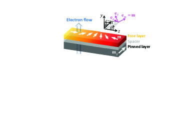
Figure 1: (Color online) Sketch of a LNSV with CPP configuration, which is a three-layer structure: a pinned FM layer ($\mathbf{m}_{\mathrm{p}}$, polarizer), a NM metallic spacer and a free FM layer ($\mathbf{m}$). A DW in the free layer is driven to move along the long axis of LNSV by perpendicularly injected currents. ($\mathbf{e}_{x},\mathbf{e}_{y},\mathbf{e}_{z}$) is the global Cartesian coordinate system, and ($\mathbf{e}_{\mathbf{m}},\mathbf{e}_{\theta},\mathbf{e}_{\phi}$) forms the local spherical coordinate system associated with $\mathbf{m}$.

The normalized magnetization $\mathbf{m}$ of the free layer can be fully described by its polar angle $\theta$ and azimuthal angle $\phi$. The associated local spherical coordinate system is denoted as ($\mathbf{e}_{\mathbf{m}},\mathbf{e}_{\theta},\mathbf{e}_{\phi}$). Then $\mathbf{m}_{\mathrm{p}}$ is decomposed into

$$\mathbf{m}_{\mathrm{p}}=p_{\mathbf{m}}\mathbf{e}_{\mathbf{m}}+p_{\theta}\mathbf{e}_{\theta}+p_{\phi}\mathbf{e}_{\phi},$$ (1)

with

$$\begin{split}p_{\mathbf{m}}&=\sin\theta_{\mathrm{p}}\cos(\phi-\phi_{\mathrm{p}})\sin\theta+\cos\theta_{\mathrm{p}}\cos\theta,\\ p_{\theta}&=\sin\theta_{\mathrm{p}}\cos(\phi-\phi_{\mathrm{p}})\cos\theta-\cos\theta_{\mathrm{p}}\sin\theta,\\ p_{\phi}&=-\sin\theta_{\mathrm{p}}\sin(\phi-\phi_{\mathrm{p}}),\end{split}$$ (2)

where $\theta_{\mathrm{p}}$ ($\phi_{\mathrm{p}}$) is the polar (azimuthal) angle of $\mathbf{m}_{\mathrm{p}}$.

The magnetic energy of the free layer includes the exchange, crystalline anisotropy, magnetostatic and FLT-induced effective potential. Following He’s workHe_EPJB_2013 , we have

$$\mathcal{E}[\mathbf{m}]=\mathcal{E}_{0}[\mathbf{m}]-\mu_{0}M_{s}^{2}\xi_{\mathrm{CPP}}\frac{J_{e}}{J_{\mathrm{p}}}\frac{b_{\mathrm{p}}}{c_{\mathrm{p}}}\ln(1+c_{\mathrm{p}}p_{\mathbf{m}}),$$ (3)

with

$$\mathcal{E}_{0}[\mathbf{m}]=J\left(\frac{\partial\mathbf{m}}{\partial z}\right)^{2}+\mu_{0}M_{s}^{2}\left(-\frac{1}{2}k_{\mathrm{E}}m_{z}^{2}+\frac{1}{2}k_{\mathrm{H}}m_{y}^{2}\right),$$ (4)

in which the magnetostatic energy has been described by local quadratic terms of $M_{x,y,z}$ by means of three average demagnetization factorsjlu_PRB_2016 . $J$ is the exchange stiffness, $\mu_{0}$ is the vacuum permeability, $\xi_{\mathrm{CPP}}$ describes the relative strength of FLT over SLT, $k_{\mathrm{E}}(k_{\mathrm{H}})$ is the total anisotropy coefficient along the easy (hard) axis of the free layer and $M_{s}$ is the saturation magnetization. In addition, $J_{\mathrm{p}}\equiv 2\mu_{0}edM_{s}^{2}/\hbar$ where $d$ is the thickness of free layer, $e(>0)$ is the absolute charge of electron and $P$ is the spin polarization of the current. At last, the two dimensionless parameters $b_{\mathrm{p}}=4P^{3/2}/[3(1+P)^{3}-16P^{3/2}]$ and $c_{\mathrm{p}}=(1+P)^{3}/[3(1+P)^{3}-16P^{3/2}]$ reproduce Slonczewski’s original spin polarization factor $g\equiv[-4+(1+P)^{3}(3+\mathbf{m}\cdot\mathbf{m}_{\mathrm{p}})/(4P^{3/2})]^{-1}$Slonczewski_JMMM_1996 by $g=b_{\mathrm{p}}/(1+c_{\mathrm{p}}p_{\mathbf{m}})$.

The magnetization dynamics in the free layer is described by the Lagrangian $L=\int\mathcal{L}\mathrm{d}^{3}\mathbf{r}$ with density

$$\mathcal{L}=\frac{\mu_{0}M_{s}}{\gamma_{0}}\dot{\phi}\cdot(1-\cos\theta)-\mathcal{E},$$ (5)

in which $\gamma_{0}=\mu_{0}\gamma$ with $\gamma$ being the gyromagnetic ratio and a dot means $\partial/\partial t$. To include the Gilbert damping and the SLT-induced anti-damping processes, an extra dissipation functional $F=\int\mathcal{F}\mathrm{d}^{3}\mathbf{r}$ is introduced with density

$$\frac{\mathcal{F}}{\mu_{0}M_{s}^{2}}=\frac{\alpha}{2}\frac{\dot{\theta}^{2}+\dot{\phi}^{2}\sin^{2}\theta}{\gamma_{0}M_{s}}-g\frac{J_{e}}{J_{\mathrm{p}}}(p_{\theta}\sin\theta\dot{\phi}-p_{\phi}\dot{\theta}).$$ (6)

The corresponding generalized Eular-Lagrangian equation

$$\frac{\mathrm{d}}{\mathrm{d}t}\left(\frac{\delta\mathcal{L}}{\delta\dot{X}}\right)-\frac{\delta\mathcal{L}}{\delta X}+\frac{\delta\mathcal{F}}{\delta\dot{X}}=0,$$ (7)

provides dynamical descriptions of TDWs, where $X$ represents related collective coordinates.

Early simulations confirmed that in FM nanostrips with small enough cross section, transverse DWs (TDWs) have the lowest energy among all meta-stable statesMcMichael_IEEE_1997 ; Thiaville_JMMM_2005 . In 2012, further simulations revealed that the stability range of TDW in free layers of LNSVs can be shifted towards larger cross section compared with monolayer strips, due to a magnetostatic screening effect between the free and pinned layersPizzini_APL_2012 . Therefore the configuration space of DWs in this work is the TDW with generalized Walker profileWalker_JAP_1974

$$\ln\tan\frac{\vartheta(z,t)}{2}=\eta\frac{z-q(t)}{\Delta(t)},\quad\phi(z,t)\equiv\varphi(t),$$ (8)

in which $\eta=+1$ or $-1$ represents head-to-head (HH) or tail-to-tail (TT) TDWs, respectively. Note that in many 1D collective-coordinate analysis, the tilting angle $\varphi(t)$ and wall center position $q(t)$ [or wall velocity $\dot{q}(t)$] are the two collective coordinates meanwhile assuming fixed wall width $\Delta(t)$Boone_PRL_2010_theo ; Tatara_JPDAP_2011 . However, the wall width does change considerably as the wall tilting angle varies if the material is magnetically biaxial. Even for uniaxial materials, the strip geometry will induce an effective hard axis in the normal direction perpendicular to strip plane. Based on these facts, we therefore view the wall width as the third collective coordinate.

In Eq. (7), by letting $X$ take $q(t)$, $\varphi(t)$, $\Delta(t)$ successively, and integrating over the long axis (i.e. $\int_{-\infty}^{+\infty}\mathrm{d}z$), we obtain the following dynamic equations

$$\frac{\dot{\varphi}+\alpha\eta\dot{q}/\Delta}{\gamma_{0}M_{s}} =b_{\mathrm{p}}\frac{J_{e}}{J_{\mathrm{p}}}\left[p_{\varphi}U(\varphi)-\frac{\xi_{\mathrm{CPP}}}{2c_{\mathrm{p}}}\ln\frac{1-c_{\mathrm{p}}\cos\theta_{\mathrm{p}}}{1+c_{\mathrm{p}}\cos\theta_{\mathrm{p}}}\right],$$ (9a)

$$\frac{\alpha\dot{\varphi}-\eta\dot{q}/\Delta}{\gamma_{0}M_{s}} =b_{\mathrm{p}}\frac{J_{e}}{J_{\mathrm{p}}}\left[\xi_{\mathrm{CPP}}p_{\varphi}U(\varphi)+\frac{1}{2c_{\mathrm{p}}}\ln\frac{1-c_{\mathrm{p}}\cos\theta_{\mathrm{p}}}{1+c_{\mathrm{p}}\cos\theta_{\mathrm{p}}}\right]$$

$$\qquad-k_{\mathrm{H}}\sin\varphi\cos\varphi,$$ (9b)

$$\frac{\pi^{2}\alpha}{6\gamma_{0}M_{s}}\frac{\dot{\Delta}}{\Delta} =b_{\mathrm{p}}\frac{J_{e}}{J_{\mathrm{p}}}\left[\xi_{\mathrm{CPP}}W(\varphi)-p_{\varphi}U(\varphi)\ln\frac{1-c_{\mathrm{p}}\cos\theta_{\mathrm{p}}}{1+c_{\mathrm{p}}\cos\theta_{\mathrm{p}}}\right]$$

$$\qquad+\left(\frac{l_{0}^{2}}{\Delta^{2}}-k_{\mathrm{E}}-k_{\mathrm{H}}\sin^{2}\varphi\right).$$ (9c)

with

$$\begin{split}U(\varphi)&\equiv\chi/\sqrt{1-c_{\mathrm{p}}^{2}\left[\sin^{2}\theta_{\mathrm{p}}\cos^{2}(\varphi-\phi_{\mathrm{p}})+\cos^{2}\theta_{\mathrm{p}}\right]},\\ W(\varphi)&\equiv\frac{1}{2c_{\mathrm{p}}}\left[\frac{\pi^{2}}{4}+\frac{1}{4}\ln^{2}\frac{1-c_{\mathrm{p}}\cos\theta_{\mathrm{p}}}{1+c_{\mathrm{p}}\cos\theta_{\mathrm{p}}}-\chi^{2}\right],\\ \chi&\equiv\arccos\frac{c_{\mathrm{p}}\sin\theta_{\mathrm{p}}\cos(\varphi-\phi_{\mathrm{p}})}{\sqrt{1-c_{\mathrm{p}}^{2}\cos^{2}\theta_{\mathrm{p}}}},\end{split}$$ (10)

and $l_{0}\equiv\sqrt{2J/(\mu_{0}M_{s}^{2})}$ being the exchange length of the free layer. Note that in the definition of function $W(\varphi)$ in Eq. (10), our calculation supports an additional “1/2” factor compared with He’s original work.

III III. DW dynamics under planar-transverse polarizers

For planar-transverse polarizers, $\theta_{\mathrm{p}}=\pi/2$ and $\phi_{\mathrm{p}}=0$. The dynamical equations evolve to

$$\frac{1+\alpha^{2}}{\gamma_{0}M_{s}\sin\varphi}\frac{\eta\dot{q}}{\Delta} =\left[k_{\mathrm{H}}\cos\varphi-(\alpha-\xi_{\mathrm{CPP}})b_{\mathrm{p}}\frac{J_{e}}{J_{\mathrm{p}}}\widetilde{U}(\varphi)\right],$$ (11a)

$$\frac{1+\alpha^{2}}{\gamma_{0}M_{s}\sin\varphi}\dot{\varphi} =-\left[(1+\alpha\xi_{\mathrm{CPP}})b_{\mathrm{p}}\frac{J_{e}}{J_{\mathrm{p}}}\widetilde{U}(\varphi)+\alpha k_{\mathrm{H}}\cos\varphi\right],$$ (11b)

$$\frac{\pi^{2}\alpha}{6\gamma_{0}M_{s}}\frac{\dot{\Delta}}{\Delta} =\left(\frac{l_{0}^{2}}{\Delta^{2}}-k_{\mathrm{E}}-k_{\mathrm{H}}\sin^{2}\varphi\right)+\xi_{\mathrm{CPP}}b_{\mathrm{p}}\frac{J_{e}}{J_{\mathrm{p}}}\widetilde{W}(\varphi),$$ (11c)

in which

$$\begin{split}\widetilde{U}(\varphi)&=\frac{\tilde{\chi}}{\sqrt{1-c_{\mathrm{p}}^{2}\cos^{2}\varphi}},\quad\widetilde{W}(\varphi)=\frac{1}{2c_{\mathrm{p}}}\left(\frac{\pi^{2}}{4}-\tilde{\chi}^{2}\right),\\ \tilde{\chi}&=\arccos(c_{\mathrm{p}}\cos\varphi).\end{split}$$ (12)

For steady traveling-wave mode, $\dot{\varphi}=0$ and $\dot{\Delta}=0$. This leads to two branches of solution:

$$\begin{split}\varphi_{0}&=n\pi,\quad v_{0}=0,\\ \Delta(\varphi_{0})&=l_{0}\left[k_{\mathrm{E}}-\xi_{\mathrm{CPP}}b_{\mathrm{p}}\frac{J_{e}}{J_{\mathrm{p}}}\widetilde{W}(\varphi_{0})\right]^{-1/2},\end{split}$$ (13)

and

$$\begin{split}\cos\varphi^{\prime}_{0}&=-\frac{1+\alpha\xi_{\mathrm{CPP}}}{\alpha k_{\mathrm{H}}}b_{\mathrm{p}}\frac{J_{e}}{J_{\mathrm{p}}}\widetilde{U}(\varphi^{\prime}_{0}),\\ v^{\prime}_{0}&=\frac{\eta\Delta(\varphi^{\prime}_{0})\gamma_{0}k_{\mathrm{H}}M_{s}}{1+\alpha\xi_{\mathrm{CPP}}}\sin\varphi^{\prime}_{0}\cos\varphi^{\prime}_{0},\\ \Delta(\varphi^{\prime}_{0})&=l_{0}\left[k_{\mathrm{E}}+k_{\mathrm{H}}\sin^{2}\varphi^{\prime}_{0}-\xi_{\mathrm{CPP}}b_{\mathrm{p}}\frac{J_{e}}{J_{\mathrm{p}}}\widetilde{W}(\varphi^{\prime}_{0})\right]^{-\frac{1}{2}}.\end{split}$$ (14)

For the first branch in Eq. (13), For the variation $\varphi=\varphi_{0}+\delta\varphi$, Eq. (11b) provides

$$\begin{split}\frac{\partial(\ln\delta\varphi)}{\partial t}&=-\frac{\gamma_{0}M_{s}}{1+\alpha^{2}}\bigg{\{}(-1)^{n}(1+\alpha\xi_{\mathrm{CPP}})b_{\mathrm{p}}\frac{J_{e}}{J_{\mathrm{p}}}\times\\ &\quad(1-c_{\mathrm{p}}^{2})^{-1/2}\arccos\left[(-1)^{n}c_{\mathrm{p}}\right]+\alpha k_{\mathrm{H}}\bigg{\}}.\end{split}$$ (15)

The stability of $\varphi_{0}-$solution requires the terms in curly braces to be positive. This leads to $J_{e}/J_{\mathrm{p}}>j_{\mathrm{d}}$ ($n$ is even) or $J_{e}/J_{\mathrm{p}}<j_{\mathrm{u}}$ ($n$ is odd), where

$$\begin{split}j_{\mathrm{u}}&\equiv\frac{\alpha k_{\mathrm{H}}}{1+\alpha\xi_{\mathrm{CPP}}}\cdot\frac{\sqrt{1-c_{\mathrm{p}}^{2}}}{b_{\mathrm{p}}\arccos(-c_{\mathrm{p}})},\\ j_{\mathrm{d}}&\equiv-\frac{\alpha k_{\mathrm{H}}}{1+\alpha\xi_{\mathrm{CPP}}}\cdot\frac{\sqrt{1-c_{\mathrm{p}}^{2}}}{b_{\mathrm{p}}\arccos(c_{\mathrm{p}})}.\end{split}$$ (16)

For the wall width of this branch, first its existence demands that when $n$ is even (odd), $J_{e}/J_{\mathrm{p}}<j_{\Delta\mathrm{u}}$ ($J_{e}/J_{\mathrm{p}}>j_{\Delta\mathrm{d}}$) with

$$\begin{split}j_{\Delta\mathrm{u}}&\equiv\frac{k_{\mathrm{E}}}{\xi_{\mathrm{CPP}}}\cdot\frac{2c_{\mathrm{p}}}{b_{\mathrm{p}}}\cdot\left(\frac{\pi^{2}}{4}-\arccos^{2}c_{\mathrm{p}}\right)^{-1},\\ j_{\Delta\mathrm{d}}&\equiv-\frac{k_{\mathrm{E}}}{\xi_{\mathrm{CPP}}}\cdot\frac{2c_{\mathrm{p}}}{b_{\mathrm{p}}}\cdot\left[\arccos^{2}(-c_{\mathrm{p}})-\frac{\pi^{2}}{4}\right]^{-1}.\end{split}$$ (17)

Since $\alpha\ll 1$ and $\xi_{\mathrm{CPP}}\ll 1$, $|j_{\Delta\mathrm{u(d)}}|\gg|j_{\mathrm{u(d)}}|$ and is usually out of experimental accessibility. Thus only $j_{\mathrm{u(d)}}$ is considered when dealing with stability issue. For the variation $\Delta=\Delta(\varphi_{0})+\delta\Delta$, Eq. (11c) provides

$$\frac{\pi^{2}\alpha}{6\gamma_{0}M_{s}}\frac{\partial(\ln\delta\Delta)}{\partial t}=-\frac{2l_{0}^{2}}{\Delta^{2}(\varphi_{0})},$$ (18)

implying a stable wall width of this solution branch (see violet solid lines in Fig. 2).

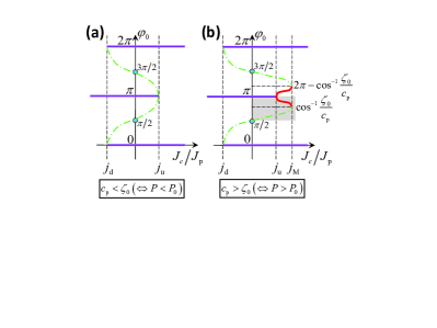
Figure 2: (Color online) Illustration of the solution branch in Eq. (14): (a) $c_{\mathrm{p}}<\zeta_{0}$, (b) $c_{\mathrm{p}}>\zeta_{0}$. In both cases, violet solid lines represent the stable solution branch in Eq. (13) with zero velocity, and green dash-dot curves represent the unstable part of solution branch in Eq. (14). In addition, red solid curves in (b) indicate the stable part of solution branch in Eq. (14). The shaded area in (b) will be calculated in details in Fig. 3.

Next we turn to the branch in Eq. (14). By rewriting the first equation as $J_{e}/J_{\mathrm{p}}=-\alpha k_{\mathrm{H}}\cos\varphi^{\prime}_{0}(1-c_{\mathrm{p}}^{2}\cos^{2}\varphi^{\prime}_{0})^{1/2}/[(1+\alpha\xi_{\mathrm{CPP}})b_{\mathrm{p}}\arccos(c_{\mathrm{p}}\cos\varphi^{\prime}_{0})]$ and analyzing its monotonicity, the permitted current density range of this branch can be obtained. Note that $J_{e}(\varphi^{\prime}_{0})=J_{e}(2\pi-\varphi^{\prime}_{0})$, we then focus on $\varphi^{\prime}_{0}\in[0,\pi]$ thus $\sin\varphi^{\prime}_{0}\geq 0$. After standard calculus, one has

$$\frac{\mathrm{d}}{\mathrm{d}\varphi^{\prime}_{0}}\left(\frac{J_{e}}{J_{\mathrm{p}}}\right)=\frac{\alpha k_{\mathrm{H}}\sin\varphi^{\prime}_{0}}{(1+\alpha\xi_{\mathrm{CPP}})b_{\mathrm{p}}}\cdot\frac{f(\zeta)}{\sqrt{1-\zeta^{2}}\cdot\arccos^{2}\zeta},$$ (19)

with

$$f(\zeta)=\left(1-2\zeta^{2}\right)\arccos\zeta+\zeta\sqrt{1-\zeta^{2}},\;\;\zeta\equiv c_{\mathrm{p}}\cos\varphi^{\prime}_{0}.$$ (20)

On the other hand, the counterpart of Eq. (15) for this solution branch is

$$\frac{\partial(\ln\delta\varphi^{\prime})}{\partial t}=\frac{\alpha\gamma_{0}M_{s}k_{\mathrm{H}}\sin^{2}\varphi^{\prime}_{0}}{(1+\alpha^{2})(1-\zeta^{2})\arccos\zeta}f(\zeta),$$ (21)

The monotonicity analysis on $f(\zeta)$ provides us a critical value $\zeta_{0}=-0.6256$ ($\Leftrightarrow P_{0}=0.3704$)He_EPJB_2013 . When $c_{\mathrm{p}}<\zeta_{0}$ ($\Leftrightarrow P<P_{0}$), $f(\zeta)>0$. This fact has two consequences: from Eq. (19), $J_{e}/J_{\mathrm{p}}$ is an increasing function on $\varphi^{\prime}_{0}\in[0,\pi]$ thus acquires its minimum ($j_{\mathrm{d}}$) at $\varphi^{\prime}_{0}=0$ and maximum ($j_{\mathrm{u}}$) at $\varphi^{\prime}_{0}=\pi$ (see Fig. 2(a)). However, Eq. (21) tells us that now this whole branch remains unstable thus is not physically preferred. When $c_{\mathrm{p}}>\zeta_{0}$ ($\Leftrightarrow P>P_{0}$), $f(\zeta)$ first increases when $\varphi^{\prime}_{0}$ runs from 0 to $\arccos(\zeta_{0}/c_{\mathrm{p}})$ and then decreases when $\varphi^{\prime}_{0}$ exceeds $\arccos(\zeta_{0}/c_{\mathrm{p}})$ to $\pi$. Correspondingly, $J_{e}/J_{\mathrm{p}}$ increases from $j_{\mathrm{d}}$ to $j_{\mathrm{M}}=0.2172\alpha k_{\mathrm{H}}/[(1+\alpha\xi_{\mathrm{CPP}})b_{\mathrm{p}}c_{\mathrm{p}}]$ and then decreases to $j_{\mathrm{u}}$, as illustrated in Fig. 2(b). Meantime, from Eq. (21) only when $\arccos(\zeta_{0}/c_{\mathrm{p}})<\varphi^{\prime}_{0}<2\pi-\arccos(\zeta_{0}/c_{\mathrm{p}})$ the solution branch in Eq. (14) is stable, which has been marked by red curves in Fig. 2(b).

Now we explain what happens physically when the CPP current density $J_{e}$ increases from 0 to large positive value. If the wall initially lies in easy $xz-$plane with $\varphi|_{t=0}=0$, i.e. the magnetization at wall center is parallel to the polarizer, then it always stays in this state with zero velocity no matter how large $J_{e}$ is. While if the wall initially lies with $\varphi|_{t=0}=\pi$, i.e. the magnetization at wall center is anti-parallel to the polarizer, it keeps on staying in this state until $J_{e}/J_{\mathrm{p}}$ increases to $j_{\mathrm{u}}$. When $J_{e}$ is further enhanced a little bit, something interesting happens. When the polarizer is not strong enough ($P<P_{0}$), the wall “jumps” to $\varphi=0$ state (through $\pi\rightarrow 0$ or $\pi\rightarrow 2\pi$ route depending on the nature of external disturbances) and then keeps still. On the contrary, if the polarizer is strong enough ($P_{0}<P\leq 1$), the wall will evolve into one of the two stable parts of the solution branch in Eq. (14). Likely, which one it runs into is determined by the nature of external disturbances. As $J_{e}/J_{\mathrm{p}}$ increases from $j_{\mathrm{u}}$ to $j_{\mathrm{M}}$, the wall acquires a finite velocity as shown by the second equation of Eq. (14). When $J_{e}/J_{\mathrm{p}}$ exceeds $j_{\mathrm{M}}$, the wall jumps to its nearest static branch under external disturbance and then keeps in this state.

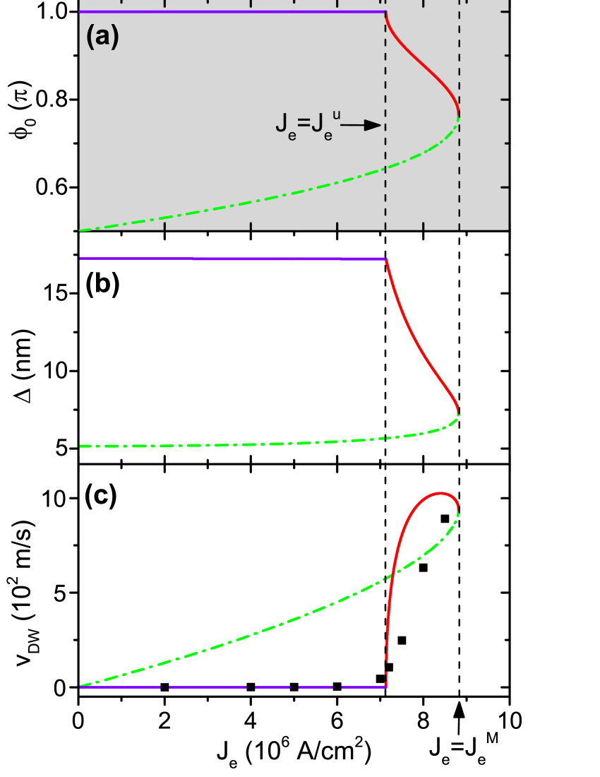
Figure 3: (Color online) Dependence of the tilting angle (a), width (b) and velocity (c) of a TDW with $\eta=-1$ on current density in a LNSV with CPP configuration and planar-transverse polarizer ($\mathbf{m}_{\mathrm{p}}=\mathbf{e}_{x}$). The subfigure (a) corresponds to the shaded area in Fig. 2(b). The free FM layer has the geometry of $50\times 3\times 8000$ $\mathrm{nm}^{3}$, with $M_{s}=1400$ kA/m, $J=30\times 10^{-12}$ J/m and $\alpha=0.007$. In addition, $P=0.6$ and $\xi_{\mathrm{CPP}}=0.1$ for spin-transfer process. The violet solid lines are the stable static branch in Eq. (13). The red solid (green dash-dot) curves comes from the stable (unstable) part of the finite-velocity branch in Eq. (14). Solid squares comes from OOMMF simulations.

Next we do some numerical estimations. The following magnetic parameters for Co are adopted (same as those in Ref. Khvalkovskiy_PRL_2009 ): $M_{s}=1400$ kA/m, $J=30\times 10^{-12}$ J/m, $\alpha=0.007$ and $\xi_{\mathrm{CPP}}=0.1$. Thus the exchange length $l_{0}=4.94$ nm. The geometry of free layer is $3\times 50\times 8000$ $\mathrm{nm}^{3}$, resulting in three average demagnetization factors: $D_{y}=0.917251$, $D_{x}=0.082269$ and $D_{z}=0.000480$. The crystalline anisotropy and edge roughness are both neglected, thus $k_{\mathrm{E}}=D_{x}-D_{z}=0.081789$ and $k_{\mathrm{H}}=D_{y}-D_{x}=0.834982$. Then $\Delta_{0}=l_{0}/\sqrt{k_{\mathrm{E}}}=17.3$ nm. As indicated, to obtain stable propagating walls the spin polarization $P$ should satisfy $P>P_{0}=0.3704$. Here we take $P=0.6$ as an example. Then $b_{\mathrm{p}}=0.3832$ and $b_{\mathrm{p}}=0.8442$, thus the extremal point is $\varphi_{0}^{\mathrm{M}}=\arccos(\zeta_{0}/c_{\mathrm{p}})=0.7657\pi$. The upper limit of the current density for the stable static branch in Eq. (13) is $J_{e}^{\mathrm{u}}=j_{\mathrm{u}}\cdot J_{\mathrm{p}}=7.13\times 10^{6}$ $\mathrm{A/cm^{2}}$. Meantime, the upper limit of the current density for the stable finite-velocity branch in Eq. (14) is $J_{e}^{\mathrm{M}}=j_{\mathrm{M}}\cdot J_{\mathrm{p}}=8.82\times 10^{6}$ $\mathrm{A/cm^{2}}$. These two values are both not high for real applications. Then the tilting angle, width and velocity of a TT ($\eta=-1$) TDW corresponding to the shaded area in Fig. 2(b) are calculated and plotted in Fig. 3. We focus on the red curves which are the stable part of the finite-velocity branch in Eq. (14). Interestingly, at $J_{e}\approx 8.40\times 10^{6}$ $\mathrm{A/cm^{2}}$ the wall can propagate along the LNSV at a velocity as high as 1025 m/s. Therefore planar-transverse polarizers have comparable current efficiency as perpendicular polarizersKhvalkovskiy_PRL_2009 . To our knowledge, this has never been reported before in existing studies.

Another attracting quantity is the high “differential mobility” ($\mathrm{d}v/\mathrm{d}J_{e}$) around $J_{e}=J_{e}^{\mathrm{u}}$ ($\varphi^{\prime}_{0}=\pi$), as shown by the red curve in Fig. 3(c). From Eq. (19), this infinity comes from the divergent behavior of $|\mathrm{d}\varphi^{\prime}_{0}/\mathrm{d}J_{e}|\propto 1/|\sin\varphi^{\prime}_{0}|\rightarrow+\infty$ at $J_{e}=J_{e}^{\mathrm{u}}$ ($\varphi^{\prime}_{0}=\pi$). Consequently, combining with Eq. (14), we have $|\mathrm{d}v^{\prime}_{0}/\mathrm{d}J_{e}|=|(\mathrm{d}v^{\prime}_{0}/\mathrm{d}\varphi^{\prime}_{0})\cdot(\mathrm{d}\varphi^{\prime}_{0}/\mathrm{d}J_{e})|\propto|\cos 2\varphi^{\prime}_{0}/\sin\varphi^{\prime}_{0}|\rightarrow+\infty$. This means that a slight increase of $J_{e}$ above $J_{e}^{\mathrm{u}}$ will lead to considerable increase of wall velocity.

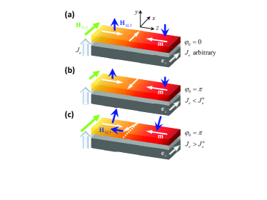
Figure 4: (Color online) Illustration of the physical mechanism responsible for the high differential mobility around $J_{e}^{\mathrm{u}}$. (a) $\phi_{0}=0$ and $J_{e}$ is arbitrary. (b) $\phi_{0}=\pi$ and $J_{e}<J_{e}^{\mathrm{u}}$. (c) $\phi_{0}=\pi$ and $J_{e}>J_{e}^{\mathrm{u}}$. In all sketches, $\eta=-1$. Green (blue) arrows represent $\mathbf{H}_{\mathrm{FLT}}$ ($\mathbf{H}_{\mathrm{SLT}}$).

To make sure this high differential mobility around $J_{e}=J_{e}^{\mathrm{u}}$ is a real effect rather than theoretical illusion, we perform numerical simulations using the OOMMF packageOOMMF with the “Xf_STT” class embedded which enables simulation on injection of multiple spin currents into a ferromagnet in OOMMF. The resulting velocities are depicted by solid squares in Fig. 3(c). The magnetic and geometric parameters are exactly the same with theoretical deductions. In particular, the crystalline anisotropy and edge roughness are both neglected and the demagnetization is turned on. As preparation, a static TDW with $\eta=-1$ and $\phi^{\prime}_{0}=\pi$ is generated at the wire center. Perpendicularly injected current density $-J_{e}\mathbf{e}_{y}$ manipulates the TDW dynamics. First, a current density pulse with strength $3.0\times 10^{7}$ $\mathrm{A/cm^{2}}$ and duration 2.5 ns is applied to slightly push the wall away from its potential valley ($\varphi^{\prime}_{0}=\pi$). Then typical current densities ($\leq 8.5\times 10^{6}$ $\mathrm{A/cm^{2}}$) are applied and the wall velocities in stable traveling-wave mode are recorded. Numerical data show that when $J_{e}<7.0\times 10^{6}$ $\mathrm{A/cm^{2}}$, the wall creeps forward for a distance and then stops. When $J_{e}\geq 7.0\times 10^{6}$ $\mathrm{A/cm^{2}}$, the wall acquires high velocity very quickly as $J_{e}$ increases. This critical current density is very close to the theoretical prediction $J_{e}^{\mathrm{u}}=7.13\times 10^{6}$ $\mathrm{A/cm^{2}}$. At $J_{e}=8.5\times 10^{6}$ $\mathrm{A/cm^{2}}$, the wall velocity is around 900 m/s which is comparable with the theoretical maximum (1025 m/s at $8.4\times 10^{6}$ $\mathrm{A/cm^{2}}$). The difference between theoretical curve and simulation data comes from the fact that around $J_{e}^{\mathrm{u}}$ the half wire with limited length (4 $\mathrm{\mu}$m) is not enough for the wall to converge to its stable solution (14).

In fact, this large differential mobility can be understood physically. By putting Eqs. (5) and (6) into the generalized Eular-Lagrangian equation (7) with $X=\theta(\phi)$, we obtain the familiar Landau-Lifshitz-Gilbert (LLG) equation

$$\begin{split}\frac{\partial\mathbf{m}}{\partial t}=&-\gamma_{0}\mathbf{m}\times\mathbf{H}^{0}_{\mathrm{eff}}+\alpha\mathbf{m}\times\frac{\partial\mathbf{m}}{\partial t}\\ &\quad-\gamma_{0}a_{J}\mathbf{m}\times(\mathbf{m}\times\mathbf{m}_{\mathrm{p}})-\gamma_{0}b_{J}\mathbf{m}\times\mathbf{m}_{\mathrm{p}},\end{split}$$ (22)

where $a_{J}=\hbar J_{e}g/(2\mu_{0}deM_{s})$, $b_{J}=\xi_{\mathrm{CPP}}a_{J}$, and $\mathbf{H}^{0}_{\mathrm{eff}}=-(\mu_{0}M_{s})^{-1}\delta\mathcal{E}_{0}/\delta\mathbf{m}$. We denote the two effective fields related to SLT and FLT as $\mathbf{H}_{\mathrm{SLT}}=a_{J}(\mathbf{m}\times\mathbf{m}_{\mathrm{p}})$ and $\mathbf{H}_{\mathrm{FLT}}=b_{J}\mathbf{m}_{\mathrm{p}}$, respectively. Note that Eq. (22) describes a gyrational magnetization dynamics accompanied by a damping-induced motion towards the effective field. For planar-transverse polarizers ($\mathbf{m}_{\mathrm{p}}=\mathbf{e}_{x}$), $\mathbf{H}_{\mathrm{FLT}}$ is always a uniform transverse field directed along $+\mathbf{e}_{x}$ thus can not induce TDW motion along $\mathbf{e}_{z}$. However, it breaks the two-fold symmetry in $x-$direction: TDWs lying in $\varphi_{0}=0$ plane are always stable while at some critical current density ($J_{e}^{\mathrm{u}}$) TDWs initially lying in $\varphi_{0}=\pi$ plane will climb out of this potential valley formed by finite hard anisotropy in $y-$direction.

When $J_{e}<J_{e}^{\mathrm{u}}$, TDWs are still lying in $\varphi_{0}=n\pi$ valleys. Thus $\mathbf{H}_{\mathrm{SLT}}$ is perpendicularly to $\varphi_{0}=n\pi$ planes and directed oppositely about the wall center [see Fig. 4(a) and 4(b)]. The gyration around $\mathbf{H}_{\mathrm{SLT}}$ leads to temporary wall displacement. At the same time, the damping process results in the tilting of magnetization towards $\mathbf{H}_{\mathrm{SLT}}$. Correspondingly, magnetic charges appear at the opposite sides of the free layer and thus generate a magnetostatic field that balances $\mathbf{H}_{\mathrm{SLT}}$. As a result, the wall stops and becomes static.

For TDWs initially lying in $\varphi_{0}=\pi$ valley and $J_{e}$ slightly exceeds $J_{e}^{\mathrm{u}}$, due to the symmetry about $\varphi_{0}=\pi$ plane, the magnetization at wall center departs from it randomly. By denoting the new stable azimuthal angle as $\varphi^{\prime}_{0}$ and from the famous “Stoner-Wohlfarth asteroid” theoremTannous_2008 , at critical point one has $H_{\mathrm{FLT}}\propto\cos\varphi^{\prime 3}_{0}$ which leads to $|\mathrm{d}\varphi^{\prime}_{0}/\mathrm{d}J_{e}|\propto|\mathrm{d}\varphi^{\prime}_{0}/\mathrm{d}H_{\mathrm{FLT}}|\propto 1/|\sin\varphi^{\prime}_{0}|\gg 1$. This explains the high differential mobility around $J_{e}^{\mathrm{u}}$. Now we take $0<\varphi^{\prime}_{0}<\pi$ as an example [see Fig. 4(c)], in wall region $\mathbf{H}_{\mathrm{SLT}}$ has $-\mathbf{e}_{z}$ component. For $\eta=-1$, this leads to a finite velocity along $+\mathbf{e}_{z}$ which explains the stable branch in Eq. (14). When current density is too large ($>J_{e}^{\mathrm{M}}$), the generalized Walker profile will collapse due to the anti-directed $\mathbf{H}_{\mathrm{SLT}}$ on the two sides of TDW and vortex/antivortex may emerge which is out of the scope of this work.

In summary, dynamical behaviors of TDWs under planar-transverse polarizers in LNSVs with CPP configuration are quite different from known results in two aspects. First, in all well-investigated current-driven stack setups, including FM monolayers (CIP), FM/heavy-metal bilayers (CIP) and LNSVs with parallel and perpendicular polarizers (CPP), TDWs have a finite mobility in the entire range of current density when dealing with a sufficiently smooth and even sample (absence of intrinsic pinning due to imperfectness). This means TDWs will acquire a steady motion with finite velocity under finite charge current density, no matter how small the latter is. However in LNSVs with strong enough planar-transverse polarizers, steady wall motion with finite velocity can only occur when driving current exceeds a finite threshold of density. Second, at the onset of wall excitation, the differential mobility is very high due to the sudden change in steady tilting angle of TDWs as current density exceeds its lower limit a little bit. This allows TDWs to acquire high velocities under small current densities. The resulting current efficiency is comparable with that of perpendicular polarizers. When the current density exceeds its upper limit, TDWs jump to their nearest static branch. These two exotic behaviors should open new possibilities for developing magnetic nanodevices based on TDW propagation with low energy consumption: (a) When polarizers of LNSVs are made of magnetic materials with in-plane rather than perpendicular magnetic anisotropy, high current efficiency is still achievable as long as they are made planar-transverse. (b) The high differential mobility around $J_{e}^{\mathrm{u}}$ makes these LNSVs candidates for high-sensitivity switches, etc.

IV IV. DW dynamics under parallel and perpendicular polarizers

The simulation work by Khvalkovskiy et. al. proposed the high current efficiency in LNSVs under parallel and perpendicular polarizers with “$\mathbf{m}\cdot\mathbf{m}_{\mathrm{p}}$-independent” STT coefficientsKhvalkovskiy_PRL_2009 . Except for numerics, they also provided a 1D analysis for parallel polarizers in which the wall velocity and tilting angle are two collective coordinates. However, for perpendicular polarizers the corresponding 1D analysis is absent. Meantime, their simulations revealed that under perpendicular (parallel) polarizers pure SLT (FLT) induces persistent wall displacement while pure FLT (SLT) does not. Therefore they conjectured that at low currents the large difference for the wall velocities between perpendicular and planar polarizers is related to the factor $\xi_{\mathrm{CPP}}$ between the torques. However, the exact ratio of mobilities for these two cases under low currents is not provided. In this section, we perform systematic Lagrangian analysis and provide answers to these issues.

IV.1 IV.A Modified Lagrangian and dynamical equations

For $\mathbf{m}\cdot\mathbf{m}_{\mathrm{p}}$-independent STT coefficients, the energy density functional turns to

$$\widetilde{\mathcal{E}}[\mathbf{m}]=\mathcal{E}_{0}[\mathbf{m}]-\mu_{0}M_{s}\tilde{b}_{J}p_{\mathbf{m}},$$ (23)

and the dissipation functional becomes

$$\frac{\widetilde{\mathcal{F}}}{\mu_{0}M_{s}^{2}}=\frac{\alpha}{2}\frac{\dot{\theta}^{2}+\dot{\phi}^{2}\sin^{2}\theta}{\gamma_{0}M_{s}}-\frac{\tilde{a}_{J}}{M_{s}}(p_{\theta}\sin\theta\dot{\phi}-p_{\phi}\dot{\theta}),$$ (24)

where $\tilde{a}_{J}=\hbar J_{e}P/(2\mu_{0}deM_{s})$ and $\tilde{b}_{J}=\xi_{\mathrm{CPP}}\tilde{a}_{J}$. Still, the generalized Walker profile is taken as the configuration space of walls. After putting the wall center position $q(t)$, tilting angle $\varphi(t)$ and width $\Delta(t)$ into Eq. (7) successively, and integrating over $z\in(-\infty,+\infty)$, a new set of dynamical equations are obtained

$$\alpha\eta\frac{\dot{q}}{\Delta}+\dot{\varphi} =\gamma_{0}\left(\frac{\pi}{2}\tilde{a}_{J}p_{\varphi}+\tilde{b}_{J}\cos\theta_{\mathrm{p}}\right),$$ (25a)

$$\eta\frac{\dot{q}}{\Delta}-\alpha\dot{\varphi} =\gamma_{0}M_{s}k_{\mathrm{H}}\sin\varphi\cos\varphi$$

$$\qquad+\gamma_{0}\left(\tilde{a}_{J}\cos\theta_{\mathrm{p}}-\frac{\pi}{2}\tilde{b}_{J}p_{\varphi}\right),$$ (25b)

$$\frac{\pi^{2}\alpha}{6}\frac{\dot{\Delta}}{\Delta} =\gamma_{0}M_{s}\left(\frac{l_{0}^{2}}{\Delta^{2}}-k_{\mathrm{E}}-k_{\mathrm{H}}\sin^{2}\varphi\right)$$

$$\qquad+\gamma_{0}\pi\tilde{b}_{J}\sin\theta_{\mathrm{p}}\cos(\varphi-\phi_{\mathrm{p}}).$$ (25c)

IV.2 IV.B Parallel polarizers

For systematicness, we first briefly revisit TDW dynamics under parallel polarizers. In this case, $\mathbf{m}_{\mathrm{p}}=\mathbf{e}_{z}$, thus $\theta_{\mathrm{p}}=0$ and then $p_{\varphi}=0$. The dynamical equations turn to

$$\frac{1+\alpha^{2}}{\gamma_{0}}\frac{\eta\dot{q}}{\Delta} =\frac{k_{\mathrm{H}}M_{s}}{2}\sin 2\varphi+(\tilde{a}_{J}+\alpha\tilde{b}_{J}),$$ (26a)

$$\frac{1+\alpha^{2}}{\gamma_{0}}\dot{\varphi} =-\frac{\alpha k_{\mathrm{H}}M_{s}}{2}\sin 2\varphi+(\tilde{b}_{J}-\alpha\tilde{a}_{J}),$$ (26b)

$$\frac{\pi^{2}\alpha}{6\gamma_{0}M_{s}}\frac{\dot{\Delta}}{\Delta} =\frac{l_{0}^{2}}{\Delta^{2}}-k_{\mathrm{E}}-k_{\mathrm{H}}\sin^{2}\varphi.$$ (26c)

The first two equations reproduce Eq. (4) in Khvalkovskiy’s work (see Ref. Khvalkovskiy_PRL_2009 ) and the third one provides the TDW width. For traveling-wave mode of TDW, $\dot{\varphi}=0$ and $\dot{\Delta}=0$. This leads to a FLT-determined steady wall velocity

$$\begin{split}v_{0}&=\frac{\eta\Delta(\varphi_{0})\gamma_{0}\xi_{\mathrm{CPP}}\tilde{a}_{J}}{\alpha},\\ \sin 2\varphi_{0}&=\frac{2(\xi_{\mathrm{CPP}}-\alpha)\tilde{a}_{J}}{\alpha M_{s}k_{\mathrm{H}}},\\ \Delta_{1}(\varphi_{0})&=l_{0}(k_{\mathrm{E}}+k_{\mathrm{H}}\sin^{2}\varphi_{0})^{-1/2}.\end{split}$$ (27)

For variation of $\varphi_{0}$, we have

$$\frac{\partial(\ln\delta\varphi_{0})}{\partial t}=-\frac{\alpha\gamma_{0}M_{s}k_{\mathrm{H}}\cos 2\varphi_{0}}{2(1+\alpha^{2})}.$$ (28)

When $\cos 2\varphi_{0}>0$, i.e. $|\varphi_{0}-n\pi|<\pi/4$, the $\varphi_{0}-$solution is stable. On the other hand, for variation of $\Delta_{1}$, one has

$$\frac{\pi^{2}\alpha}{6\gamma_{0}M_{s}}\frac{\partial(\delta\Delta)}{\partial t}=-\frac{2l_{0}^{2}}{\Delta_{1}^{2}(\varphi_{0})}\delta\Delta-\Delta_{1}(\varphi_{0})k_{\mathrm{H}}\sin 2\varphi_{0}\delta\varphi_{0}.$$ (29)

Thus the wall width should be stable as long as $\varphi_{0}$ is stable.

Next we compare our analytics with existing simulation data. The geometry and magnetic parameters of the free layer are the same as those in the end of Sec. II, except that the spin polarization is changed to $P=0.32$ (same as in Khvalkovskiy’s work). By requiring $|\sin 2\varphi_{0}|\leq 1$, the Walker limit (under which traveling-wave mode survives) is $J_{\mathrm{W}}=\alpha M_{s}k_{\mathrm{H}}/(2\kappa|\xi_{\mathrm{CPP}}-\alpha|)=2.20\times 10^{8}$ $\mathrm{A/cm^{2}}$. However this is just theoretical prediction based on the generalized Walker profile. Real simulations (see Fig. 1(b) of Ref. Khvalkovskiy_PRL_2009 ) revealed that TDWs disappear due to global-spin-transfer-induced domain excitation when $J_{e}>2.4\times 10^{7}$ $\mathrm{A/cm^{2}}$ which is an order of magnitude smaller $J_{\mathrm{W}}$. Thus in traveling-wave mode, at most $\sin^{2}\varphi_{0}\sim 10^{-2}$ and $\Delta_{1}(\varphi_{0})\sim\Delta_{0}=17.3$ nm. This leads to a constant wall mobility $\sim 1.09\times 10^{-5}$ $\mathrm{(m/s)/(A/cm^{2})}$, which perfectly explains the linear dependence of wall velocity on current density in Fig. 1(b) of Ref. Khvalkovskiy_PRL_2009 . In Fig. 5 of our work, analytical results from Eq. (27) are plotted by solid curves. Meantime, numerical data from Fig. 1(b) in Ref. Khvalkovskiy_PRL_2009 are indicated by solid squares. Obviously as long as TDWs exist ($J_{e}<2.4\times 10^{7}$ $\mathrm{A/cm^{2}}$), our theoretical results are in good agreement with numerical simulations.

Figure 5: Dependence of the tilting angle (a), width (b) and velocity (c) of a TDW on current density in a LNSV with CPP configuration and parallel polarizer ($\mathbf{m}_{\mathrm{p}}=\mathbf{e}_{z}$). The geometry and magnetic parameters of the free layer are the same as those in Fig. 3, except that the spin polarization is changed to $P=0.32$. The solid curves are from Eq. (27) and the solid squares in (c) are from Fig. 1(b) in Ref. Khvalkovskiy_PRL_2009 with exactly the same geometric and magnetic parameters.

IV.3 IV.C Perpendicular polarizers

Now $\mathbf{m}_{\mathrm{p}}=\mathbf{e}_{y}$, thus $\theta_{\mathrm{p}}=\pi/2$ and $\phi_{\mathrm{p}}=\pi/2$. Then $p_{\varphi}=\cos\varphi$ and Eq. (25) is simplified to

$$\frac{1+\alpha^{2}}{\gamma_{0}}\frac{\eta\dot{q}}{\Delta} =\left[k_{\mathrm{H}}M_{s}\sin\varphi+\frac{\pi}{2}(\alpha\tilde{a}_{J}-\tilde{b}_{J})\right]\cos\varphi,$$ (30a)

$$\frac{1+\alpha^{2}}{\gamma_{0}}\dot{\varphi} =\left[\frac{\pi}{2}(\tilde{a}_{J}+\alpha\tilde{b}_{J})-\alpha k_{\mathrm{H}}M_{s}\sin\varphi\right]\cos\varphi,$$ (30b)

$$\frac{\pi^{2}\alpha}{6\gamma_{0}M_{s}}\frac{\dot{\Delta}}{\Delta} =\left(\frac{l_{0}^{2}}{\Delta^{2}}-k_{\mathrm{E}}-k_{\mathrm{H}}\sin^{2}\varphi\right)+\frac{\pi\tilde{b}_{J}}{M_{s}}\sin\varphi.$$ (30c)

For steady traveling-wave mode, we need $\dot{\varphi}=0$ and $\dot{\Delta}=0$. This leads to two branches of solution:

$$\varphi_{0}=\left(n+\frac{1}{2}\right)\pi,\quad v_{0}=0,$$

$$\Delta_{2}(\varphi_{0})=l_{0}\left[k_{\mathrm{E}}+k_{\mathrm{H}}-(-1)^{n}\frac{\pi\tilde{b}_{J}}{M_{s}}\right]^{-1/2},$$ (31)

and

$$\begin{split}\sin\varphi^{\prime}_{0}&=\frac{\pi}{2}\frac{1+\alpha\xi_{\mathrm{CPP}}}{\alpha}\frac{\tilde{a}_{J}}{k_{\mathrm{H}}M_{s}},\\ v^{\prime}_{0}&=\frac{\pi}{2}\frac{\eta\Delta_{2}(\varphi^{\prime}_{0})\gamma_{0}\tilde{a}_{J}}{\alpha}\cos\varphi^{\prime}_{0},\\ \Delta_{2}(\varphi^{\prime}_{0})&=l_{0}\left(k_{\mathrm{E}}+k_{\mathrm{H}}\sin^{2}\varphi^{\prime}_{0}-\frac{\pi\tilde{b}_{J}}{M_{s}}\sin\varphi^{\prime}_{0}\right)^{-1/2}.\end{split}$$ (32)

Then we perform stability analysis to these two branches. For the one in Eq. (IV.3), after taking variation of $\varphi_{0}$ and substituting it into Eq. (30b), one has

$$\frac{\partial(\ln\delta\varphi_{0})}{\partial t}=-\frac{\alpha\gamma_{0}M_{s}k_{\mathrm{H}}}{1+\alpha^{2}}\left[\frac{\pi}{2}\left(\frac{1}{\alpha}+\xi_{\mathrm{CPP}}\right)\frac{(-1)^{n}\tilde{a}_{J}}{k_{\mathrm{H}}M_{s}}-1\right].$$ (33)

Then we define $J_{1}\equiv 4|\xi_{\mathrm{CPP}}-\alpha|\pi^{-1}(1+\alpha\xi_{\mathrm{CPP}})^{-1}J_{\mathrm{W}}$. When $J_{e}>J_{1}$ ($n$ is even) or $J_{e}<-J_{1}$ ($n$ is odd), $(-1)^{n}(\alpha^{-1}+\xi_{\mathrm{CPP}})\tilde{a}_{J}\pi/(2k_{\mathrm{H}}M_{s})-1>0$ always holds thus the $\varphi_{0}=(n+1/2)\pi$ solution in the first branch is stable. For the wall width of this branch, similar variational analysis provides the same result as in Eq. (18), implying that the static solution at $\varphi_{0}=(n+1/2)\pi$ always has a stable wall width.

Then we move to the other branch in Eq. (32). The solution $\varphi^{\prime}_{0}$ requires $|\sin\varphi^{\prime}_{0}|\leq 1$, which is equivalent to $|J_{e}|\leq J_{1}$. After varying $\varphi^{\prime}_{0}$ by $\delta\varphi^{\prime}$ and putting into Eq. (30b), we have

$$\frac{\partial(\ln\delta\varphi^{\prime})}{\partial t}=-\frac{\alpha\gamma_{0}M_{s}k_{\mathrm{H}}\cos^{2}\varphi^{\prime}_{0}}{1+\alpha^{2}},$$ (34)

implying that $\varphi^{\prime}_{0}-$solution is always stable. The corresponding TDW velocity can be explicitly written out as

$$v^{\prime}_{0}=\frac{\pi}{2}\frac{\eta\Delta_{2}(\varphi^{\prime}_{0})\gamma_{0}\tilde{a}_{J}}{\alpha}(-1)^{m}\sqrt{1-\left(\frac{\pi}{2}\frac{1+\alpha\xi_{\mathrm{CPP}}}{\alpha k_{\mathrm{H}}M_{s}}\tilde{a}_{J}\right)^{2}},$$ (35)

in which “$(-1)^{m}$” comes from the initial condition ($\varphi^{\prime}_{0}|_{t=0}=m\pi$ at $t=0$). For $|J_{e}|\ll J_{1}$, one has

$$v^{\prime}_{0}\approx\frac{\pi}{2}\frac{\eta\Delta_{0}\gamma_{0}\tilde{a}_{J}}{\alpha}(-1)^{m}.$$ (36)

Clearly it has a mobility larger than that of “parallel-polarizer” case [see Eq. (27)] by a factor of $\pi/(2\xi_{\mathrm{CPP}})\approx 15.7$, thus well explains the higher current efficiency of perpendicular polarizers. When $|J_{e}|\rightarrow J_{1}$, the $\varphi^{\prime}_{0}-$solution converges to $\varphi_{0}-$branch with zero wall velocity.

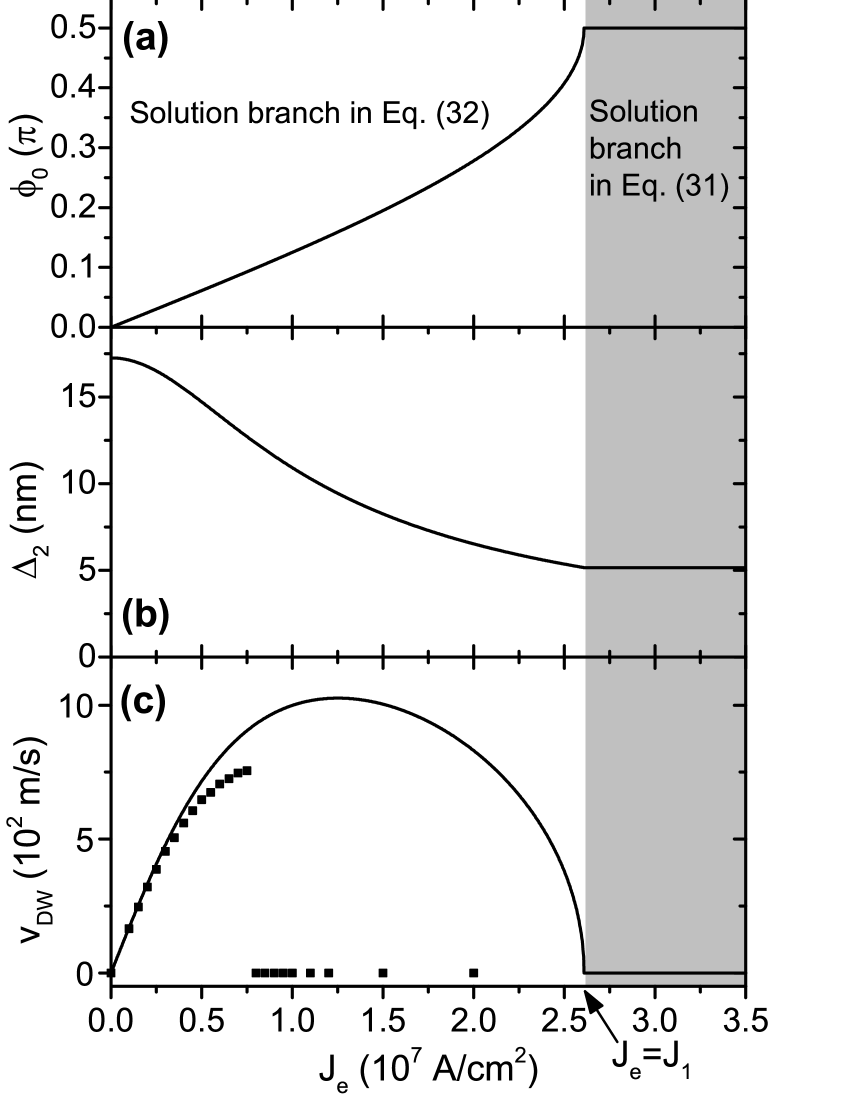
Figure 6: Dependence of the tilting angle (a), width (b) and velocity (c) of a TDW on current density in a LNSV with CPP configuration and perpendicular polarizer ($\mathbf{m}_{\mathrm{p}}=\mathbf{e}_{y}$). The geometry and magnetic parameters of the free layer are the same as those in Fig. 5. The solid curves in the white-background area are the solution branch in Eq. (32) and the solid lines in the shaded area are those from Eq. (IV.3). The solid squares in (c) are from Fig. 2(b) in Ref. Khvalkovskiy_PRL_2009 .

For the same magnetic parameters as in parallel polarizers, $J_{1}=0.1183J_{\mathrm{W}}=2.61\times 10^{7}$ $\mathrm{A/cm^{2}}$. For HH TDWs ($\eta=+1$) and standard initial condition ($\varphi_{0}|_{t=0}=\varphi^{\prime}_{0}|_{t=0}=0$), the solution branch in Eq. (IV.3) [Eq. (32)] is plotted in Fig. 6 by solid line (curve) in shaded (white-background) area. In addition, simulation data from Fig. 2(b) in Ref. Khvalkovskiy_PRL_2009 are depicted in our Fig. 6(c) by solid squares. Clearly when $J_{e}\leq 0.3\times 10^{7}$ $\mathrm{A/cm^{2}}$, our analytics coincides with simulation data very well. For larger current density, the wall configuration in simulations will be distorted from the standard Walker profile due to global spin transfers, thus leads to the inconsistency between analytics and simulations.

IV.4 IV.D Comparison with experimental data

As mentioned in Sec. I, to our knowledge there are two groups of experimental work. In the first group, currents with definite density inject perpendicularly into LNSVs or half-ring MTJs (genuine CPP configurations). While in the second group, in-plane current flows through ZigZag LNSVs and the “vertical spin current” is suggested to be the source of DW velocity boosting, however the corresponding spin current density is hard to estimate. Therefore we focus on the first group in which genuine CPP configuration with definite current density is under investigation. Furthermore, our analytics is obtained in a strip geometry (resulting in three averaged demagnetization factors, and hence $k_{\mathrm{E}}$ and $k_{\mathrm{H}}$), thus can not directly apply to half-ring geometry. In summary, the best case to make the comparison is the first case in the first group, which is the experimental work by Boone et. al. in 2010Boone_PRL_2010_exp on LNSVs with parallel polarizers.

In their work, the free layer is made of the nickel-rich nickel-iron alloy (NRNIA) with $M_{s}=430$ kA/m and the crystalline anisotropy is neglected. Its geometry ($3\times 90\times 5000$ $\mathrm{nm}^{3}$) provides three average demagnetization factors: $D_{y}=0.9473$, $D_{x}=0.05182$ and $D_{z}=0.00088$. Thus we have $k_{\mathrm{E}}=D_{x}-D_{z}=0.0509$ and $k_{\mathrm{H}}=D_{y}-D_{x}=0.8955$. The resulting coercive force is $k_{\mathrm{E}}M_{s}=275$ Oe, which is consistent with experimental measurements (NRNIA reversal at $+200$ and $-300$ Oe) in Fig. 2(b) of Ref. Boone_PRL_2010_exp . The exchange stiffness ($J$) has not been explicitly provided. However from the fixed wall width ($\lambda=53$ nm) they adopted in simulations, we have $J=\mu_{0}k_{\mathrm{E}}M_{s}^{2}\lambda^{2}/2=16.6\times 10^{-12}$ J/m. Furthermore, the conversion coefficient from current density to SLT strength is $\kappa=\tilde{a}_{J}/J_{e}=\hbar P/(2\mu_{0}deM_{s})=1.32\times 10^{-3}$ $\mathrm{(A/m)/(A/cm^{2})}$ for $P=0.65$. Now we estimate the wall mobility under small driving currents where the wall width can be viewed as constant ($\lambda=53$ nm). Note that they obtained a damping coefficient from a fitting to the rectified voltage with zero-FLT assumption. However as indicated by Khvalkovskiy et. al., FLT is crucial for TDW dynamics in LNSVs with parallel polarizers. Therefore we adopt the typical NRNIA value $\alpha=0.01$ rather than their fitting parameter. Moreover, we assume $\xi_{\mathrm{CPP}}=0.1$ which is the maximum permissible in Ref. Boone_PRL_2010_exp . From Eq. (27), the wall mobility is $|v_{0}/J_{e}|=\lambda\gamma_{0}\xi_{\mathrm{CPP}}\kappa/\alpha=1.55\times 10^{-4}$ $\mathrm{(m/s)/(A/cm^{2})}$. This agrees well with their experimental data for $J_{e}<2\times 10^{6}$ $\mathrm{A/cm^{2}}$ in their Fig. 4(b). On the other hand, the fitting result $\alpha=0.09$ leads to a wall mobility of $1.72\times 10^{-5}$ $\mathrm{(m/s)/(A/cm^{2})}$. This is an order of magnitude smaller than the experimental observations thus should be abandoned.

V V. Further boosting by UTMFs

In real magnetic nondevices composed of LNSVs, to further boost TDWs’ propagation, a UTMF

$$\mathbf{H}_{\mathrm{TMF}}=H_{\perp}(\cos\Phi_{\perp},\sin\Phi_{\perp},0)$$ (37)

can be applied, with $H_{\perp}$ and $\Phi_{\perp}$ being its strength and orientation, respectively. Meanwhile, the pinned layer is assumed to be unaffected which is a harmless simplification and will not affect our main conclusion. Nevertheless, rigorous profile and velocity of TDWs under an arbitrary UTMF are hard to obtain due to the mismatch between symmetries in different energy terms in transverse direction. Since we focus on the traveling-mode at low current density, the 1D-AEMGoussev_PRB_2013 ; Goussev_Royal_2013 ; jlu_PRB_2016 ; jlu_SciRep_2017 ; jlu_Nanomaterials_2019 on LLG equation shall provide useful information. Recalling the results in Sec. III, for TDWs moving under planar-transverse polarizers, 1D-AEM is not applicable since stable wall motion with finite velocity can only be excited for current density exceeding a finite threshold. Hence in this section, we present the results for parallel and perpendicular polarizers.

V.1 V.A Parallel polarizers

The 1D-AEM needs static profiles of TDWs as the basis to calculate the response of the system under external stimuli. Depending on UTMF strength, static TDWs take different profiles. Therefore we discuss the “small UTMF” and “finite UTMF” cases separately.

For small UTMFs, the CCP current density, UTMF, and inverse of time are rescaled simultaneously, that is $\tilde{a}_{J}=\epsilon\tilde{a}_{J}^{0}$, $\tilde{b}_{J}=\epsilon\tilde{b}_{J}^{0}$, $H_{\perp}=\epsilon h_{\perp}$ and $1/t=\epsilon(1/\tau)$, where $\epsilon$ is the rescaling infinitesimal. The real solution of the LLG equation is expanded as $\Omega(z,t)=\Omega_{0}(z,\tau)+\epsilon\Omega_{1}(z,\tau)+O(\epsilon^{2})$ with $\Omega=\theta,\phi$. Putting them back into the original LLG equation (22), the solution to the zeroth-order equation is the Walker ansatz. At the first order of $\epsilon$, with the help of zeroth-order solutions, the differential equation about $\theta_{1}$ reads,

$$\begin{split}F_{\mathrm{s}}&=\mathcal{L}\theta_{1},\quad\mathcal{L}\equiv\frac{2J}{\mu_{0}M_{s}}\left(-\frac{\mathrm{d}^{2}}{\mathrm{d}z^{2}}+\frac{\theta^{\prime\prime\prime}_{0}}{\theta^{\prime}_{0}}\right),\\ F_{\mathrm{s}}&\equiv\left[\frac{\eta\alpha(z_{0})_{\tau}}{\gamma_{0}\Delta_{0}}-\tilde{b}_{J}^{0}\right]\sin\theta_{0}+(-1)^{n}h_{\perp}\cos\theta_{0}\cos\Phi_{\perp},\end{split}$$ (38)

where $(z_{0})_{\tau}\equiv\mathrm{d}z_{0}/\mathrm{d}\tau$ and a prime means $\mathrm{d}/\mathrm{d}z$. The subscript “s” indicates the “small UTMF” case. Note that $\mathcal{L}$ is the same 1D self-adjoint Schrödinger operator as given in Refs. Goussev_PRB_2013 ; Goussev_Royal_2013 ; jlu_PRB_2016 ; jlu_SciRep_2017 ; jlu_Nanomaterials_2019 . Following the “Fredholm alternative”, by demanding $\theta^{\prime}_{0}$ (kernel of $\mathcal{L}$) to be orthogonal to the function $F_{\mathrm{s}}$ defined in Eq. (38), TDW velocity in traveling-wave mode under small UTMFs is

$$V_{\mathrm{s}}=\epsilon(z_{0})_{\tau}=\eta\gamma_{0}\Delta_{0}\tilde{b}_{J}/\alpha,$$ (39)

which reproduces the rigorous result in Eq. (27).

For finite UTMFs, we rescale the current density and the TDW velocity ($V_{\mathrm{f}}$) simultaneously, i.e. $\tilde{a}_{J}=\epsilon\tilde{a}_{J}^{0}$, $\tilde{b}_{J}=\epsilon\tilde{b}_{J}^{0}$ and $V_{\mathrm{f}}=\epsilon v$ in which the subscript “f” denotes the “finite UTMF” case. By introducing the traveling coordinate $\tilde{z}\equiv z-V_{\mathrm{f}}t=z-\epsilon vt$, $\theta(z,t)$ and $\phi(z,t)$ are expanded as $\Omega(z,t)=\Omega_{0}(\tilde{z})+\epsilon\Omega_{1}(\tilde{z})+O(\epsilon^{2})$ with $\Omega=\theta,\phi$. Substituting them into the LLG equation, an approximate polar angle profile $\theta_{0}$ (solution to the zeroth-order equations) of the wall is obtained

$$\ln\frac{\sin\theta_{0}-\sin\theta_{\infty}}{1+\cos(\theta_{0}+\theta_{\infty})}=\frac{\eta\tilde{z}}{\Delta(\phi_{\infty})/\cos\theta_{\infty}},\quad$$ (40)

with

$$\begin{split}\phi_{\infty}&=\tan^{-1}\left[k_{\mathrm{E}}\tan\Phi_{\perp}/(k_{\mathrm{E}}+k_{\mathrm{H}})\right],\\ \theta_{\infty}&=\sin^{-1}\frac{H_{\perp}}{M_{s}\sqrt{k_{\mathrm{E}}^{2}\cos^{2}\phi_{\infty}+(k_{\mathrm{E}}+k_{\mathrm{H}})^{2}\sin^{2}\phi_{\infty}}},\\ \Delta(\phi_{\infty})&=l_{0}\left(k_{\mathrm{E}}+k_{\mathrm{H}}\sin^{2}\phi_{\infty}\right)^{-1/2},\end{split}$$ (41)

in which $\theta_{\infty}$ ($\phi_{\infty}$) is the polar (azimuthal) angle of magnetization in domains. At the first order of $\epsilon$, after similar process as in field-driven casejlu_PRB_2016 , the equation about $\theta_{1}$ is

$$\mathcal{L}(\theta_{1})=F_{\mathrm{f}}\equiv v\gamma_{0}^{-1}(\alpha\theta^{\prime}_{0}-\sin\theta_{0}\phi^{\prime}_{0})-\tilde{b}_{J}^{0}\sin\theta_{0}.$$ (42)

where a “prime” means $\mathrm{d}/\mathrm{d}\tilde{z}$. Again, $\theta^{\prime}_{0}$ (kernel of $\mathcal{L}$) should be orthogonal to the function $F_{\mathrm{f}}$. After similar calculation, TDW velocity in traveling-wave mode under finite UTMF is,

$$\begin{split}V_{\mathrm{f}}&=u(\theta_{\infty})\frac{\eta\gamma_{0}\Delta(\phi_{\infty})\tilde{b}_{J}}{\alpha},\\ u(\theta_{\infty})&=\frac{2\cos\theta_{\infty}}{2\cos\theta_{\infty}-(\pi-2\theta_{\infty})\sin\theta_{\infty}}.\end{split}$$ (43)

This clearly shows that UTMFs can boost TDW propagation by a factor $u(\theta_{\infty})$, which has been well studied in Ref. jlu_PRB_2016 .

V.2 V.B Perpendicular polarizers

For small UTMFs, after similar rescaling, expansion and substitution operations, the differential equation about $\theta_{1}$ is,

$$\mathcal{L}\theta_{1}=\frac{\eta\alpha(z_{0})_{\tau}\sin\theta_{0}}{\gamma_{0}\Delta_{0}}+(-1)^{n}\left(h_{\perp}\cos\theta_{0}\cos\Phi_{\perp}-\tilde{a}_{J}^{0}\right).$$ (44)

The corresponding wall velocity is,

$$V_{\mathrm{s}}=\epsilon(z_{0})_{\tau}=(-1)^{n}\eta\pi\gamma_{0}\Delta_{0}\tilde{a}_{J}/(2\alpha),$$ (45)

which is the $\varphi^{\prime}_{0}\rightarrow n\pi$ limit of Eq. (32).

For finite UTMFs, the equation about $\theta_{1}$ is

$$\mathcal{L}\theta_{1}=\frac{v}{\gamma_{0}}(\alpha\theta^{\prime}_{0}-\sin\theta_{0}\phi^{\prime}_{0})-\tilde{a}_{J}^{0}\cos\phi_{0}+\tilde{b}_{J}^{0}\cos\theta_{0}\sin\phi_{0}.$$ (46)

The existence condition of $\theta_{1}-$solution provides

$$\begin{split}V_{\mathrm{f}}&\approx\omega(\theta_{\infty})\frac{\eta\gamma_{0}\Delta(\phi_{\infty})\tilde{a}_{J}}{\alpha}\cos\phi_{\infty},\\ \omega(\theta_{\infty})&=\frac{\pi-2\theta_{\infty}}{2\cos\theta_{\infty}-(\pi-2\theta_{\infty})\sin\theta_{\infty}}.\end{split}$$ (47)

Simple calculus shows that $\omega(\theta_{\infty})$ has similar divergent behavior as $u(\theta_{\infty})$ when $H_{\perp}\rightarrow H_{\perp}^{\mathrm{max}}$, thus considerably boost TDW motion. Interestingly, in LNSVs with perpendicular polarizers, TDW motion can be manipulated not only by UTMF strength (via “$\omega(\theta_{\infty})$”) but also its orientation (via “$\cos\phi_{\infty}$”). This comes from the fact that polarized electrons always act as an extra time-dependent effective field in hard axis. For TDWs with $\phi_{\infty}\neq n\pi$, magnetization in wall region rotates around the effective field hence results in a translational wall displacement along “$\eta\mathbf{e}_{z}$” direction. Meanwhile, projection of SLT to the hard axis $\mathbf{e}_{y}$ contributes to “$\cos\phi_{\infty}$”. These lead to the final “$\eta\cos\phi_{\infty}$” factor in Eq. (47).

VI VI. Summary

In this work, TDW dynamics in LNSVs with CPP configurations are systematically investigated within Lagrangian framework. When STT coefficients take the Slonczewski’s original form, our results show that stable traveling-wave motion of TDWs with finite velocity can survive for strong enough planar-transverse polarizers, with the current efficiency comparable with that of perpendicular ones. More importantly, TDWs have ultra-high differential mobility around the onset of stable wall excitation. These results should provide insights for developing magnetic nanodevices with low energy consumption. For $\mathbf{m}\cdot\mathbf{m}_{\mathrm{p}}$-independent STT coefficients, analytics for parallel and perpendicular polarizers perfectly explains existing simulations and experiments. At last, further boosting of TDWs by external UTMFs are investigated with help of 1D-AEM and turns out to be efficient.

VII Acknowledgement

M. L. is supported by the Project of Hebei Province Higher Educational Science and Technology Program (QN2019309). Z. A. is funded by the Hebei Province Department of Education (GCC2014025). J. L. acknowledges the support from National Natural Science Foundation of China (Grant No. 11374088).

References

- (1) F H De Leeuw, R Van Den Doel, and U Enz, Rep. Prog. Phys. 43, 689 (1980).
- (2) Y. Tserkovnyak, A. Brataas, G. E. W. Bauer, and B. I. Halperin, Rev. Mod. Phys. 77, 1375 (2005).
- (3) M. Kläui, J. Phys.: Condens. Matter 20, 313001 (2008).
- (4) D. A. Allwood, G. Xiong, C. C. Faulkner, D. Atkinson, D. Petit, and R. P. Cowburn, Science, 309, 1688 (2005).
- (5) M. Hayashi, L. Thomas, R. Moriya, C. Rettner, and S. S. P. Parkin, Science 320, 209 (2008).
- (6) J. H. Franken, H. J. M. Swagten, and B. Koopmans, Nat. Nanotechnol. 7, 499 (2012).
- (7) J. Münchenberger, G. Reiss, and A. Thomas, J. Appl. Phys. 111, 07D303 (2012).
- (8) S. S. P. Parkin and S.-H. Yang, Nat. Nanotechnol. 10, 195 (2015).
- (9) M. Li, J. Wang, and J. Lu, New J. Phys. 21, 053011 (2019).
- (10) J. Slonczewski, J. Magn. Magn. Mater. 159, L1 (1996).
- (11) Z. Li and S. Zhang, Phys. Rev. Lett. 92, 207203 (2004).
- (12) G. Tatara, H. Kohno, and J. Shibata, Phys. Rep. 468, 213 (2008).
- (13) J. Grollier, D. Lacour, V. Cros, A. Hamzic, A. Vaurès, and A. Fert, D. Adam and G. Faini, J. Appl. Phys. 92, 4825 (2002).
- (14) J. Grollier, P. Boulenc, V. Cros, A. Hamzić, A. Vaurès, A. Fert, and G. Faini, Appl. Phys. Lett. 83, 509 (2003).
- (15) C. K. Lim, T. Devolder, C. Chappert, J. Grollier, V. Cros, A. Vaurès, A. Fert, and G. Faini, Appl. Phys. Lett. 84, 2820 (2004).
- (16) A. Rebei and O. Mryasov, Phys. Rev. B 74, 014412 (2006).
- (17) K.Kawabata, M. Tanizawa, K.Ishikawa, Y. Inoue, M.Inuishi, and T.Nishimura, presented at the 2011 International Conference on Simulation of Semiconductor Processes and Devices, 2011 (unpublished).
- (18) A. V. Khvalkovskiy, K. A. Zvezdin, Ya. V. Gorbunov, V. Cros, J. Grollier, A. Fert, and A.K. Zvezdin, Phys. Rev. Lett. 102, 067206 (2009).
- (19) C. T. Boone, J. A. Katine, M. Carey, J. R. Childress, X. Cheng, and I. N. Krivorotov, Phys. Rev. Lett. 104, 097203 (2010).
- (20) A. Chanthbouala, R. Matsumoto, J. Grollier, V. Cros, A. Anane, A. Fert, A. V. Khvalkovskiy, K. A. Zvezdin, K. Nishimura, Y. Nagamine, H. Maehara, K. Tsunekawa, A. Fukushima, and S. Yuasa, Nat. Phys. 7, 626 (2011).
- (21) P. J. Metaxas, J. Sampaio, A. Chanthbouala, R. Matsumoto, A. Anane, A. Fert, K. A. Zvezdin, K. Yakushiji, H. Kubota, A. Fukushima, S. Yuasa, K. Nishimura, Y. Nagamine, H. Maehara, K. Tsunekawa, V. Cros, and J. Grollier, Sci. Rep. 3, 1829 (2013).
- (22) J. Sampaio, S. Lequeux, P. J. Metaxas, A. Chanthbouala, R. Matsumoto, K. Yakushiji, H. Kubota, A. Fukushima, S. Yuasa, K. Nishimura, Y. Nagamine, H. Maehara, K. Tsunekawa, V. Cros, and J. Grollier, Appl. Phys. Lett. 103, 242415 (2013).
- (23) S. Pizzini, V. Uhlíř, J. Vogel, N. Rougemaille, S. Laribi, V. Cros, E. Jiménez, J. Camarero, C. Tieg, and E. Bonet, Appl. Phys. Express 2, 023003 (2009).
- (24) V. Uhlíř, S. Pizzini, N. Rougemaille, J. Novotný, V. Cros, E. Jiménez, G. Faini, L. Heyne, F. Sirotti, C. Tieg, A. Bendounan, F. Maccherozzi, R. Belkhou, J. Grollier, A. Anane, and J. Vogel, Phys. Rev. B 81, 224418 (2010).
- (25) V. Uhlíř, S. Pizzini, N. Rougemaille, V. Cros, E. Jiménez, L. Ranno, O. Fruchart, M. Urbánek, G. Gaudin, J. Camarero, C. Tieg, F. Sirotti, E. Wagner, and J. Vogel, Phys. Rev. B 83, 020406(R) (2011).
- (26) V. Uhlíř, J. Vogel, N. Rougemaille, O. Fruchart, Z. Ishaque, V. Cros, J. Camarero, J. C. Cezar, F. Sirotti, and S. Pizzini, J. Phys.: Condens. Matter 24, 024213 (2012).
- (27) P.-B. He, Eur. Phys. J. B 86, 412 (2013).
- (28) A. Goussev, R. G. Lund, J. M. Robbins, V. Slastikov, and C. Sonnenberg, Phys. Rev. B 88, 024425 (2013).
- (29) A. Goussev, R. G. Lund, J. M. Robbins, V. Slastikov, and C. Sonnenberg, Proc. R. Soc. A 469, 20130308 (2013).
- (30) J. Lu, Phys. Rev. B 93, 224406 (2016).
- (31) M. Li, J. B. Wang, and J. Lu, Sci. Rep. 7, 43065 (2017).
- (32) M. Yu, M. Li, and J. Lu, Nanomaterials 9, 128 (2019).
- (33) R. D. McMichael and M. J. Donahue, IEEE Trans. Magn. 33, 4167 (1997).
- (34) Y. Nakatani, A. Thiaville, and J. Miltat, J. Magn. Magn. Mater. 290, 750 (2005).
- (35) N. Rougemaille, V. Uhlíř, O. Fruchart, S. Pizzini, J. Vogel, and J. C. Toussaint, Appl. Phys. Lett. 100, 172404 (2012).
- (36) N. L. Schryer and L. R. Walker, J. Appl. Phys. 45, 5406 (1974).
- (37) C. T. Boone and I. N. Krivorotov, Phys. Rev. Lett. 104, 167205 (2010).
- (38) J. Shibata, G. Tatara, and H. Kohno, Journal of Physics D: Applied Physics 44, 384004 (2011).
- (39) M. J. Donahue and D. G. Porter, OOMMF User’s Guide, Version 1.0, Interagency Report NISTIR 6376 (National Institute of Standards and Technology, Gaithersburg, MD, Sept 1999; http://math.nist.gov/oommf).
- (40) C. Tannous and J. Gieraltowski, Eur. J. Phys. 29, 475 (2008).