Black holes with Lambert W function horizons

Abstract

We consider Einstein gravity with a negative cosmological constant endowed with distinct matter sources. The different models analyzed here share the following two properties: (i) they admit static symmetric solutions with planar base manifold characterized by their mass and some additional Noetherian charges, and (ii) the contribution of these latter in the metric has a slower falloff to zero than the mass term, and this slowness is of logarithmic order. Under these hypothesis, it is shown that, for suitable bounds between the mass and the additional Noetherian charges, the solutions can represent black holes with two horizons whose locations are given in term of the real branches of the Lambert W functions. We present various examples of such black hole solutions with electric, dyonic or axionic charges with AdS and Lifshitz asymptotics. As an illustrative example, we construct a purely AdS magnetic black hole in five dimensions with a matter source given by three different Maxwell invariants.

1 Introduction

The AdS/CFT correspondence has been proved to be extremely useful for getting a better understanding of strongly coupled systems by studying classical gravity, and more specifically black holes. In particular, the gauge/gravity duality can be a powerful tool for analyzing finite temperature systems in presence of a background magnetic field. In such cases, from the dictionary of the correspondence, the black holes must be endowed with a magnetic charge corresponding to the external magnetic field of the CFT. In light of this constatation, it is clear that dyonic black holes are of great importance in order to study the charge transport at quantum critical point, particulary for strongly coupled CFTs in presence of an external magnetic field. For example, four-dimensional dyonic black holes have been proved to be relevant for a better comprehension of planar condensed matter phenomena such as the quantum Hall effect [1], the superconductivity-superfluidity [2] or the Nernst effect [3]. The study of dyonic black holes is not only interesting in four dimensions, but also in higher dimensions where their holographic applications have been discussed in the current literature. For example, it has been shown that large dyonic AdS black holes are dual to stationary solutions of a charged fluid in presence of an external magnetic field [4]. In this last reference, the AdS/CFT correspondence was used conversely and stationary solutions of the Navier-Stokes equations were constructed corresponding to an hypothetical five-dimensional AdS dyonic rotating black string with nonvanishing momentum along the string. We can also mention that magnetic/dyonic black holes present some interest from a purely gravity point of view. Indeed, there is a wide range of contexts in which magnetic/dyonic solutions are currently studied including in particular supergravity models [5, 6], Einstein-Yang-Mills theory [7] or nonlinear electrodynamics [8]. Nevertheless, in spite of partial results, the problem of finding magnetic solutions in higher dimension is an highly nontrivial problem. For example, it is easy to demonstrate that under suitable hypothesis, magnetic solutions in odd dimensions $D\geq 5$ for the Einstein-Maxwell or for the Lovelock-Maxwell theories do not exist [9, 10]. This observation is in contrast with the four-dimensional situation where static dyonic configuration can be easily constructed thanks to the electromagnetic duality which rotates the electric field into the magnetic field. In the same register, one may also suspect the lack of electromagnetic duality and of the conformal invariance in dimension $D>4$ to explain the difficulty for constructing the higher-dimensional extension of the Kerr-Newmann solution.

The purpose of the present paper is twofold. Firstly, we would like to present a simple dyonic extension of the five-dimensional Reissner-Nordstrom solution with planar horizon. The solution will be magnetically charged by considering an electromagnetic source composed by at least three different Maxwell gauge fields. Each of these $U(1)$ gauge fields will be sustained by one of the three different coordinates of the planar base manifold. Interestingly enough, the magnetic contribution in the metric has an asymptotically logarithmic falloff of the form $\frac{\ln r}{r^{2}}$. Nevertheless, in spite of this slowly behavior, the thermodynamics analysis yields finite quantities even for the magnetic charge. Since we are working in five dimensions, we extend as well this dyonic solution to the case of Einstein-Gauss-Bonnet gravity. We can also mention that the causal structure of the dyonic solution can not be done analytically. Nevertheless from different simulations, one can observe that the solution has a Reissner-Nordstrom like behavior. Indeed, depending on the election of the integration constants, the solution can be a black hole with inner and outer horizons or an extremal black hole or the solution can have a naked singularity located at the origin. On the other hand, we notice that the horizon structure of the purely magnetic solution can be treated analytically. More precisely, we will show that, as for the Reissner- Nordstrom solution, the absence of naked singularity can be guaranteed for a suitable bound relation between the mass and the magnetic charge. Moreover, in this case, the location of the inner and outer horizons are expressed analytically in term of the real branches of so-called Lambert W function. This latter is defined to be the multivalued inverse of the complex function $f(\omega)=\omega e^{\omega}$ which has an infinite countable number of branches but only two of them are real-valued, see Ref. [11] for a nice review. The Lambert W functions have a wide range of applications as for example in combinatoric with the tree functions that are used in the enumeration of trees [12] or for equations with delay that have applications for biological, chemical or physical phenomena, see e. g. [13] or in the AdS/CFT correspondence as in the expression of the large-spin expansion of the energy of the Gubser-Klebanov-Polyakov string theory [14]. Just to conclude this parenthesis about the Lambert W function, we also mention that this function can be used in the case of the Schwarzschild metric as going from the Eddington-Finkelstein coordinates to the standard Schwarzschild coordinates

The plan of the paper is organized as follows. In the next section, we present our toy model for dyonic solutions which consists on the five-dimensional Einstein-Gauss-Bonnet action with three different Abelian gauge fields. For this model, we derive a dyonic black hole configuration as well as its GR limit. A particular attention will be devoted to the purely magnetic GR solution for which a bound relation between the mass and the magnetic charge ensures the existence of an event horizon covering the naked singularity. In this case, the inner and outer horizons are expressed in term of the two real branches of the Lambert W functions. We will establish that this mass bound is essentially due to the fact that the magnetic charge has a slower falloff of logarithmic order to zero than the mass term in the metric function. Starting from this observation, we will present in Sec. $3$ various examples of black holes sharing this same feature with electric, axionic or magnetic charges and with AdS and Lifshitz asymptotics. In Sec. $4$, we extend the previous solutions to general dyonic configurations with axionic charges. Finally, the last section is devoted to our conclusion and an appendix is provided where some useful properties of the Lambert W functions are given.

2 Five-dimensional dyonic black hole solution

In Refs. [9, 10], it has been proved that, under suitable hypothesis, magnetic black hole solutions for Einstein-Maxwell action in odd dimensions $D\geq 5$ can not exit. As we will show below, a simple way of circumventing this obstruction is to consider more than one Maxwell gauge field. The fact of considering various Abelian fields in order to construct dyonic black holes in five dimensions have already been considered, see Refs. [15] and [16]. More precisely, we will establish that the Einstein gravity eventually supplemented by the Gauss-Bonnet term since we are working in $D=5$ can admit dyonic black hole solutions for an electromagnetic source given at least by three different Maxwell invariants. In order to achieve this task, we consider the following action

$$S[g,{\cal A}_{I}]=\int d^{5}x\,\sqrt{-g}\Big{[}\frac{R-2\Lambda}{2}+\frac{\alpha}{2}\left(R^{2}-4\,R_{\mu\nu}R^{\mu\nu}+R_{\alpha\beta\mu\nu}R^{\alpha\beta\mu\nu}\right)-\frac{1}{4}\sum_{I=1}^{3}{\cal{F}}_{(I)\mu\nu}{\cal{F}}_{(I)}^{\mu\nu}\Big{]},$$ (2.1)

where the ${\cal{F}}_{(I)\mu\nu}$’s are the three different Maxwell field strengths associated to the $U(1)$ gauge fields ${\cal A}_{I}$ for $I=\{1,2,3\}$ and $\alpha$ represents the Gauss-Bonnet coupling constant. The field equations obtained by varying this action read

$$G_{\mu\nu}+\Lambda g_{\mu\nu}+\alpha K^{\tiny{\mbox{GB}}}_{\mu\nu}=\sum_{I=1}^{3}\left({\cal{F}}_{(I)\mu\sigma}{\cal{F}}_{(I)\nu}^{\phantom{\sigma\sigma\,}\sigma}\right)-\frac{1}{4}{g}_{\mu\nu}\sum_{I=1}^{3}\left({\cal{F}}_{(I)\sigma\rho}{\cal{F}}_{(I)}^{\sigma\rho}\right),$$

$${\nabla}_{\mu}{\cal{F}}_{(I)}^{\mu\nu}=0,\qquad\mbox{for}\quad I=\{1,2,3\},$$ (2.2)

where the variation of the Gauss-Bonnet term is given by

$$K^{\tiny{\mbox{GB}}}_{\mu\nu}=2\big{(}RR_{\mu\nu}-2R_{\mu\rho}R^{\rho}_{\,\,\nu}-2R^{\rho\sigma}R_{\mu\rho\nu\sigma}+R_{\mu}^{\,\,\rho\sigma\gamma}R_{\nu\rho\sigma\gamma}\big{)}-\frac{1}{2}\,g_{\mu\nu}\big{(}R^{2}-4R_{\rho\sigma}R^{\rho\sigma}+R_{\rho\sigma\lambda\delta}R^{\rho\sigma\lambda\delta}\big{)}.$$

In one hand, it is known that the field equations (2) with one Maxwell invariant $I=1$ admits electrically charged black holes [17] generalizing the solution of Boulware-Deser [18]. On the other hand, it is simple to prove that the magnetic extension of the Boulware-Deser solution can not exist [9, 10]. Nevertheless, as shown below, the presence of two extra Maxwell invariants renders possible the magnetic extension of the Boulware-Deser solution but only in the case of flat horizon. In fact a dyonic solution with flat horizon of the field equations (2) is found to be

$$ds^{2}=-F(r)dt^{2}+\frac{dr^{2}}{F(r)}+r^{2}\sum_{i=1}^{3}dx_{i}^{2},$$

$$F(r)=\frac{r^{2}}{4\alpha}\left[1\mp\sqrt{1+\frac{4\alpha\Lambda}{3}+{\frac{16\alpha{\cal{M}}}{3|\Sigma_{3}|{r}^{4}}}-{\frac{4\alpha{\cal{Q}}_{e}^{2}}{|\Sigma_{3}|^{2}{r}^{6}}}+\frac{8\alpha{\cal{Q}}_{m}^{2}\ln(r)}{|\Sigma_{3}|^{2}r^{4}}}\right],$$ (2.3)

$${\cal A}_{1}=-\frac{{\cal{Q}}_{e}}{2|\Sigma_{3}|r^{2}}dt+\frac{{\cal{Q}}_{m}}{|\Sigma_{3}|}x_{2}\,dx_{3},\quad{\cal A}_{2}=-\frac{{\cal{Q}}_{e}}{2|\Sigma_{3}|r^{2}}dt+\frac{{\cal{Q}}_{m}}{|\Sigma_{3}|}x_{3}\,dx_{1},$$

$${\cal A}_{3}=-\frac{{\cal{Q}}_{e}}{2|\Sigma_{3}|r^{2}}dt+\frac{{\cal{Q}}_{m}}{|\Sigma_{3}|}x_{1}\,dx_{2},$$

where ${\cal M}$, ${\cal Q}_{e}$ and ${\cal Q}_{m}$ are three integration constants corresponding respectively to the mass, the electric and the magnetic charge and $|\Sigma_{3}|$ is the finite volume of the compact $3-$dimensional flat base manifold. Various comments can be made concerning this dyonic solution. Firstly, in the absence of the magnetic charge ${\cal Q}_{m}=0$, the solution reduces to the electrically extension of the Boulware-Deser solution [17] even if there are three different Maxwell invariants. This is because each of these three invariants contributes in the same footing for the full solution, and hence one could have switch off two of them from the very beginning. The GR limit $\alpha\to 0$ of the solution concerns only the upper branch of the solution and yields to the metric function given by

$$F_{\mbox{{\tiny GR}}}(r)=-\frac{r^{2}\Lambda}{6}-\frac{2{\cal M}}{3|\Sigma_{3}|r^{2}}+\frac{{\cal Q}_{e}^{2}}{2|\Sigma_{3}|^{2}r^{4}}-\frac{{\cal Q}_{m}^{2}\ln r}{|\Sigma_{3}|^{2}r^{2}},$$ (2.4)

while the Abelian gauge fields remain identical. Computing the Kretschmann invariant, one notices that the dyonic solution in the Einstein-Gauss-Bonnet theory or its GR limit has a singularity located at the origin.

The causal structure of the dyonic solution is quite involved and can not be treated analytically as in the case of the four-dimensional Reissner-Nordstrom dyonic solution. Nevertheless, it is quite simple to see that the GR solution (2.4) with $\Lambda<0$ and without magnetic charge, has a Reissner-Nordstrom like behavior in the sense that for ${\cal M}\geq{3^{\frac{5}{3}}|{\cal Q}_{e}|^{\frac{4}{3}}\left(-\Lambda\right)^{\frac{1}{3}}}\big{/}{4^{\frac{4}{3}}|\Sigma_{3}|^{\frac{1}{3}}}$, the solution describes a (extremal) black hole while the case ${\cal M}<{3^{\frac{5}{3}}|{\cal Q}_{e}|^{\frac{4}{3}}\left(-\Lambda\right)^{\frac{1}{3}}}\big{/}{4^{\frac{4}{3}}|\Sigma_{3}|^{\frac{1}{3}}}$ will yield a naked singularity. The dyonic GR solution has also a similar behavior which can be appreciated only by means of some simulations reported in the graphics below. In the next subsection, we will see that in the purely magnetic case, the causal structure of the solution can be analyzed analytically.

To conclude this section, we mention that the GR dyonic solution (2.4) satisfies the dominant energy conditions. Indeed, it is simple to see that the energy density $\mu$, the radial pressure $p_{r}$ and the tangential pressure $p_{t}$ given by

$$\mu=\frac{3}{2|\Sigma_{3}|^{2}r^{6}}\left[{\cal Q}_{m}^{2}r^{2}+{\cal Q}_{e}^{2}\right],\qquad p_{r}=-\mu,\qquad p_{t}=\frac{1}{2|\Sigma_{3}|^{2}r^{6}}\left[{\cal Q}_{m}^{2}r^{2}+3{\cal Q}_{e}^{2}\right],$$ (2.5)

verify the dominant energy conditions

$$\mu\geq 0,\qquad-\mu\leq p_{r}\leq\mu,\qquad-\mu\leq p_{t}\leq\mu.$$ (2.6)

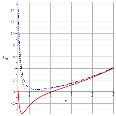
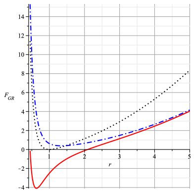
Figure 1: Plot of the metric function $F(r)$ in the GR-limit (2.4), where the left panel corresponds to the electric solution for $\Lambda=-1$ and ${\cal Q}_{e}/|\Sigma_{3}|=2/\sqrt{3}$, while the right panel is the dyonic situation with the same values of $\Lambda$ and ${\cal Q}_{e}/|\Sigma_{3}|$, together with ${\cal Q}_{m}/|\Sigma_{3}|=0.1$. For both cases, the naked singularity solution is represented by a blue dashed-dotted line, the extremal black holes with a black dashed line and the solution with inner and outer horizons by a red continuous line.

2.1 Purely magnetic GR solution

For $\alpha\to 0$ and ${\cal Q}_{e}=0$, the purely magnetic GR solution (2.4) becomes

$$ds^{2}=-F(r)dt^{2}+\frac{dr^{2}}{F(r)}+r^{2}\sum_{i=1}^{3}dx_{i}^{2},\qquad F(r)=-\frac{r^{2}\Lambda}{6}-\frac{2{\cal M}}{3|\Sigma_{3}|r^{2}}-\frac{{\cal Q}_{m}^{2}\ln r}{|\Sigma_{3}|^{2}r^{2}},$$

$${\cal A}_{1}=\frac{{\cal Q}_{m}}{|\Sigma_{3}|}x_{2}\,dx_{3},\quad{\cal A}_{2}=\frac{{\cal Q}_{m}}{|\Sigma_{3}|}x_{3}\,dx_{1},\quad\quad{\cal A}_{3}=\frac{{\cal Q}_{m}}{|\Sigma_{3}|}x_{1}\,dx_{2}.$$ (2.7)

In order to study the variations of the metric function $F$, it is useful to define

$$h(x)=6|\Sigma_{3}|^{2}r^{2}F(r)=-\Lambda|\Sigma_{3}|^{2}x-\frac{3}{2}{\cal Q}_{m}^{2}\ln x-4{\cal M}|\Sigma_{3}|,\qquad\mbox{with}\quad x=r^{4}.$$ (2.8)

For negative cosmological constant $\Lambda<0$, we have $\lim_{x\to\infty}h(x)=\lim_{x\to 0^{+}}h(x)=\infty$ and the function $h$ has a global minimum at $x=\frac{3{\cal Q}_{m}^{2}}{-2\Lambda|\Sigma_{3}|^{2}}$. The equation for the zeros of the function $h$ that will give as well the location of the horizons for the metric function $F$ through (2.8) is of the form (6.39). Hence, its corresponding discriminant as defined in Eq. (6.40) is given by

$$\Delta=\frac{2\Lambda|\Sigma_{3}|^{2}}{3{\cal Q}_{m}^{2}}e^{-\frac{8{\cal M}|\Sigma_{3}|}{3{\cal Q}_{m}^{2}}}.$$ (2.9)

Since we are considering the negative cosmological constant case $\Lambda<0$, the discriminant is negative, and as mentioned in the appendix, the equation $h(x)=0$ will have two real roots only if $\Delta\in]-\frac{1}{e},0[$. This condition in turn requires that the mass ${\cal M}$ must satisfy the following bound relation

$${\cal M}>\frac{3{\cal Q}_{m}^{2}}{8|\Sigma_{3}|}\left[1-\ln\left(\frac{3{\cal Q}_{m}^{2}}{-2\Lambda|\Sigma_{3}|^{2}}\right)\right]={\cal M}_{0}.$$ (2.10)

For ${\cal M}$ satisfying such bound, the metric function $F$ has an inner (Cauchy) horizon $r_{-}$ and an outer (event) horizon $r_{+}$ whose locations are expressed in term of the two real branches of the Lambert W functions, $W_{0}$ and $W_{-1}$ as

$$r_{-}=e^{-\frac{W_{0}(\Delta)}{4}-\frac{2{\cal M}|\Sigma_{3}|}{3{\cal Q}_{m}^{2}}},\qquad\qquad r_{+}=e^{-\frac{W_{-1}(\Delta)}{4}-\frac{2{\cal M}|\Sigma_{3}|}{3{\cal Q}_{m}^{2}}},$$ (2.11)

with $\Delta$ given by (2.9). In contrast with the four-dimensional magnetic Reissner-Nordstrom solution (or even the dyonic configuration), the bound (2.10) does not restrict the mass ${\cal M}$ to be positive. In fact, for ${\cal Q}_{m}^{2}\geq-2\Lambda|\Sigma_{3}|^{2}e/3$, the bound ${\cal M}_{0}\leq 0$, and hence the singularity at the origin can still be covered by an horizon even for a solution with a negative mass. On the other hand, for ${\cal M}$ saturating the bound (2.10), namely ${\cal M}={\cal M}_{0}$ or equivalently $\Delta=-\frac{1}{e}$, one ends up with an extremal black hole with $r_{+}=r_{-}$. Finally, for ${\cal M}<{\cal M}_{0}$, the solution will have a naked singularity. To be complete, we also mention that the energy density, the radial and tangential pressure of the purely magnetic GR solution are given by (2.5) with ${\cal Q}_{e}=0$, and hence the magnetic solution satisfies as well the dominant energy conditions (2.6).

3 Other examples of black holes with Lambert W function horizons

In the previous section, we have shown that purely magnetic black holes of five-dimensional Einstein gravity with $3$ different Abelian gauge fields exist provided a certain bound relation between the mass and the magnetic charge. In addition, the location of the horizons can be expressed thanks to the real branches of the Lambert W functions. In this section, we will present few examples enjoying these same features (bound for the mass and horizons expressed in term of the Lambert W functions) with different Noetherian charges (electric, dyonic, magnetic or axionic) and different asymptotics (AdS or Lifshitz). In order to achieve this task, it is clear from the previous analysis that the Noetherian charges in the metric must have a slower falloff of logarithmic order in comparison to the mass term. In what follows, we will present four different such solutions: an AdS dyonic black hole in five dimensions, an AdS electrically charged solution in odd dimension and two Lifshitz black holes with a magnetic and axionic charge in arbitrary dimension. These configurations are particular solutions of the following general $D-$dimensional action

$$S[g,\phi,A,{\cal A},\psi_{j}]=\int d^{D}x\sqrt{-g}\,{\cal L},$$ (3.12)

$${\cal L}=\frac{R-2\Lambda}{2}-\frac{1}{2}\partial_{\mu}\phi\partial^{\mu}\phi-\frac{1}{4}e^{\lambda\phi}\left(F_{\mu\nu}F^{\mu\nu}\right)^{q}-\frac{1}{4}\sum_{I=1}^{n}e^{\alpha_{I}\phi}{\cal{F}}_{(I)\mu\nu}{\cal{F}}_{(I)}^{\mu\nu}-\frac{1}{2}\sum_{j=1}^{D-2}e^{\beta_{j}\phi}\partial_{\mu}\psi_{j}\partial^{\mu}\psi_{j}.$$

In this action, we leave open the possibility of having a nonlinear Maxwell term $(F_{\mu\nu}F^{\mu\nu})^{q}$ where $F_{\mu\nu}=\partial_{\mu}A_{\nu}-\partial_{\nu}A_{\mu}$. Such nonlinearity has been shown to be fruitful to obtain charged solutions in different gravity contexts, see e. g. [19]. As in the previous example, in order to sustain a magnetic charge, we will also add some extra Abelian gauge fields ${\cal{F}}_{(I)\mu\nu}=\partial_{\mu}{\cal{A}}_{(I)\nu}-\partial_{\nu}{\cal{A}}_{(I)\mu}$ for $I=\{1,2,\cdots,n\}$. We justify the presence of axionic fields $\psi_{j}$ from the fact that we are looking for solutions with planar base manifold, and as shown in the fourth example or in the next section, the axionic fields perfectly accommodate an ansatz of the form $\psi_{j}=\lambda x_{j}$ where the $x_{j}$ are the planar coordinates of the base manifold (3.13). This particular ansatz for the axionic fields also provides a simple mechanism of momentum dissipation [20], and in this case the holographic DC conductivities (electrical, thermoelectric and thermal) can be expressed in terms of the black hole horizon data [21, 22]. For examples, the DC conductivities of dyonic black holes with axionic fields have been computed recently in Refs. [23]. Finally, we note that the model considered here (3.12) also allows a possible coupling of the electromagnetic fields $A$, ${\cal A}$ and the axionic fields $\psi_{j}$ to a dilaton field $\phi$.

The field equations associated to the action (3.12) read

$$G_{\mu\nu}+\Lambda g_{\mu\nu}=\Big{(}\partial_{\mu}\phi\partial_{\nu}\phi-\frac{1}{2}g_{\mu\nu}\partial_{\sigma}\phi\partial^{\sigma}\phi\Big{)}+q\,e^{\lambda\phi}\big{(}F_{\sigma\rho}F^{\sigma\rho}\big{)}^{q-1}F_{\mu\sigma}F_{\nu}^{\phantom{\,}\sigma}-\frac{g_{\mu\nu}}{4}e^{\lambda\phi}\left(F_{\sigma\rho}F^{\sigma\rho}\right)^{q}$$

$$+\sum_{I=1}^{n}e^{\alpha_{I}\phi}\left({\cal{F}}_{(I)\mu\sigma}{\cal{F}}_{(I)\nu}^{\phantom{\sigma\sigma}\sigma}-\frac{1}{4}{g}_{\mu\nu}{\cal{F}}_{(I)\sigma\rho}{\cal{F}}_{(I)}^{\sigma\rho}\right)+\sum_{j=1}^{D-2}e^{\beta_{j}\phi}\Big{(}\partial_{\mu}\psi_{j}\partial_{\nu}\psi_{j}-\frac{1}{2}g_{\mu\nu}\partial_{\sigma}\psi_{j}\partial^{\sigma}\psi_{j}\Big{)},$$

$$\nabla_{\mu}\left(e^{\lambda\phi}\big{(}F_{\sigma\rho}F^{\sigma\rho}\big{)}^{q-1}F^{\mu\nu}\right)=0,$$

$${\nabla}_{\mu}\left(e^{\alpha_{I}\phi}{\cal{F}}_{(I)}^{\mu\nu}\right)=0,$$

$$\nabla_{\mu}\left(e^{\beta_{j}\phi}\nabla^{\mu}\psi_{j}\right)=0,$$

$$\Box\phi-\frac{\lambda}{4}e^{\lambda\phi}\left(F_{(i)\sigma\rho}F_{(i)}^{\sigma\rho}\right)^{q}-\frac{1}{4}\sum_{I=1}^{n}\alpha_{I}e^{\alpha_{I}\phi}{\cal{F}}_{(I)\mu\nu}{\cal{F}}_{(I)}^{\mu\nu}-\frac{1}{2}\sum_{j=1}^{D-2}\beta_{j}e^{\beta_{j}\phi}\partial_{\mu}\psi_{j}\partial^{\mu}\psi_{j}=0,$$

and we look for a static ansatz with a planar base manifold of the form

$$ds^{2} = -N^{2}(r)F(r)dt^{2}+\frac{dr^{2}}{F(r)}+r^{2}\sum_{i=1}^{D-2}dx_{i}^{2}.$$ (3.13)

In what follows, we will derive four classes of solutions of the previous field equations, and their analysis will only be considered in the case of a negative cosmological constant $\Lambda<0$.

3.1 Electrically charged AdS black holes for nonlinear Maxwell theory in odd dimension

This case will correspond of setting $\phi={\cal{A}}_{I}=\psi_{j}=0$ in (3.12) and the Maxwell nonlinearity $q$ is of the form $q=\frac{D-1}{2}$. As shown in Ref. [24], there exists a purely electric solution with logarithmic falloff, and this solution, in order to be real, must be restricted to odd dimension $D=2k+1$ with $k\geq 1$. Hence the Maxwell nonlinearity is $q=k$ and the metric function and the electric potential are given by

$$F(r) = -\frac{r^{2}\Lambda}{k(2k-1)}-\frac{2{\cal{M}}}{(2k-1)|\Sigma_{2k-1}|r^{2k-2}}-(-2)^{k-1}\left[\frac{(-1)^{k}(2)^{1-k}{\cal{Q}}_{e}}{k|\Sigma_{2k-1}|}\right]^{\frac{2k}{2k-1}}\frac{\ln r}{r^{2k-2}},$$

$$N(r) = 1,\quad A_{0}=-\left[\frac{(-1)^{k}(2)^{1-k}{\cal{Q}}_{e}}{k|\Sigma_{2k-1}|}\right]^{\frac{1}{2k-1}}\ln r.$$ (3.14)

Here ${\cal{M}}$ is the mass, ${\cal{Q}}_{e}$ is the electric charge and $|\Sigma_{2k-1}|$ denotes the finite volume element of the compact $(2k-1)-$dimensional base manifold.

As for the previous magnetic solution, the equation determining the zeros of the metric function $F$ can be put in the form (6.39) by substituting $x=r^{2k}$ and in this case, the discriminant (6.40) is given by

$$\Delta=-\frac{|\Sigma_{2k-1}|\Lambda\,{{e}^{{\frac{2{\cal M}k}{B}}}}}{B},\qquad\mbox{with}\qquad B=\left(-2\right)^{k-2}\left(2\,k-1\right)\left[\frac{(-1)^{k}(2)^{1-k}{\cal{Q}}_{e}}{k|\Sigma_{2k-1}|}\right]^{\frac{2k}{2k-1}}|\Sigma_{2k-1}|.$$ (3.15)

We note that, because of the presence of the term $\left(-2\right)^{k-2}$, the sign of the discriminant will depend on the parity of the integer $k$. Indeed, for even $k$ or equivalently for odd dimensions $D=5\,\,\mbox{mod}\,\,4$, the discriminant is positive, and hence the solution is a black hole for any value of the mass ${\cal M}$, and there is a single horizon located at

$$r_{h}=e^{-\frac{W_{0}(\Delta)}{2k}-\frac{{\cal M}}{B}}.$$

Nevertheless, in this case, it is simple to see that the energy density is always negative, and consequently the energy conditions do not hold. On the other hand, for odd $k$ or equivalently for odd dimensions $D=3\,\,\mbox{mod}\,\,4$, the solution will be a black hole provided that the mass satisfies the following bound relation with the electric charge

$${\cal M}\geq{-\frac{B}{2k}\left[1-\ln\left(\frac{B}{\Lambda|\Sigma_{2k-1}|}\right)\right]}.$$ (3.16)

In this case, the inner and outer horizons are given by

$${r_{-}=e^{-\frac{W_{0}(\Delta)}{2k}-\frac{{\cal M}}{B}},\qquad r_{+}=e^{-\frac{W_{-1}(\Delta)}{2k}-\frac{{\cal M}}{B}}},$$ (3.17)

and the dominant energy conditions (2.6) are satisfied with

$$\mu=\frac{2^{k-2}(2k-1)}{r^{2k}}\left[\frac{(-1)^{k}(2)^{1-k}{\cal{Q}}_{e}}{k|\Sigma_{2k-1}|}\right]^{\frac{2k}{2k-1}},\qquad p_{r}=-\mu,\qquad p_{t}=\frac{2^{k-2}}{r^{2k}}\left[\frac{(-1)^{k}(2)^{1-k}{\cal{Q}}_{e}}{k|\Sigma_{2k-1}|}\right]^{\frac{2k}{2k-1}}.$$ (3.18)

3.2 Five-dimensional AdS dyonic black holes and particular stealth configuration

In five dimensions, the previous solution can be magnetically charged in such a way that the magnetic charge also appears in the metric function with a slower falloff of logarithmic order in comparison to the mass. The corresponding model that sustains such solution is given by the action (3.12) by setting $\phi=\psi_{j}=0$ and by considering $n=3$ extra gauge fields ${\cal A}_{I}$ as well as the nonlinear Maxwell term with the exponent $q=2$. In this case, the dyonic solution which can also be viewed as an electric extension of the solution (2.1) is given by the ansatz (3.13) with

$$F(r)=-\frac{\Lambda}{6}r^{2}-\frac{2{\cal M}}{3|\Sigma_{3}|r^{2}}-\frac{\ln r}{r^{2}}\left[\frac{{\cal Q}_{m}^{2}}{|\Sigma_{3}|^{2}}-\frac{2|{\cal Q}_{e}|^{\frac{4}{3}}}{\left(4|\Sigma_{3}|\right)^{\frac{4}{3}}}\right],\qquad N(r)=1,$$

$${\cal A}_{1}=\frac{{\cal Q}_{m}}{|\Sigma_{3}|}x_{2}\,dx_{3},\quad{\cal A}_{2}=\frac{{\cal Q}_{m}}{|\Sigma_{3}|}x_{3}\,dx_{1},\quad\quad{\cal A}_{3}=\frac{{\cal Q}_{m}}{|\Sigma_{3}|}x_{1}\,dx_{2},\qquad{A_{0}=-\frac{|{\cal Q}_{e}|^{\frac{1}{3}}}{\left(4|\Sigma_{3}|\right)^{\frac{1}{3}}}\ln r}.$$

Before proceeding as before, we would like to point out that the point defined by

$$|{\cal Q}_{e}|=\frac{2^{\frac{5}{4}}|{\cal Q}_{m}|^{\frac{3}{2}}}{|\Sigma_{3}|^{\frac{1}{2}}},$$ (3.19)

is very special in the sense that the metric function reduces to the Schwarzschild AdS metric with a flat horizon. This in turn implies that the field equations at the point (3.19) can be interpreted as a stealth configuration [25] defined on the Schwarzschild AdS background since both side (geometric and matter part) of the Einstein equations vanish separately, i. e.

$$G_{\mu\nu}+\Lambda g_{\mu\nu}= 0 =\sum_{I=1}^{3}\left({\cal{F}}_{(I)\mu\sigma}{\cal{F}}_{(I)\nu}^{\phantom{\sigma\sigma\,}\sigma}\right)-\frac{1}{4}{g}_{\mu\nu}\sum_{I=1}^{3}\left({\cal{F}}_{(I)\sigma\rho}{\cal{F}}_{(I)}^{\sigma\rho}\right)$$

$$+2F_{\mu\sigma}F_{\nu}^{\,\,\sigma}\left(F_{\alpha\beta}F^{\alpha\beta}\right)-\frac{1}{4}g_{\mu\nu}\left(F_{\alpha\beta}F^{\alpha\beta}\right)^{2}.$$

Note that such stealth configuration but for a dyonic four-dimensional Reissner-Nordstrom black hole was known in the case of an Abelian gauge field coupled to a particular Horndeski term [26] or for a generalized Proca field theory [27].

Outside the stealth point, the discriminant associated to the zeros of the metric function $F$ is given by

$$\Delta=\frac{2\Lambda}{3A}e^{-\frac{8{\cal M}}{3|\Sigma_{3}|A}},\qquad\mbox{with}\quad A=\frac{{\cal Q}_{m}^{2}}{|\Sigma_{3}|^{2}}-\frac{2|{\cal Q}_{e}|^{\frac{4}{3}}}{\left(4|\Sigma_{3}|\right)^{\frac{4}{3}}}.$$ (3.21)

Since, we are only considering the negative cosmological constant case, we conclude that:

1. For $A<0$, that is for

   $$|{\cal Q}_{e}|>\frac{2^{\frac{5}{4}}|{\cal Q}_{m}|^{\frac{3}{2}}}{|\Sigma_{3}|^{\frac{1}{2}}},$$

   the solution has a single horizon located at

   $$r_{h}=e^{-\frac{W_{0}(\Delta)}{4}-\frac{2{\cal M}}{3|\Sigma_{3}|A}},$$

   but the solution does not satisfy the dominant energy conditions neither the weak energy conditions since the energy density $\mu=\frac{3A}{2r^{4}}$ is always negative.

2. For $A>0$, that is for

   $$|{\cal Q}_{e}|<\frac{2^{\frac{5}{4}}|{\cal Q}_{m}|^{\frac{3}{2}}}{|\Sigma_{3}|^{\frac{1}{2}}},$$

   the solution represents a dyonic AdS black hole only if

   $${\cal M}\geq\frac{3|\Sigma_{3}|A}{8}\left[1-\ln\left(\frac{3A}{-2\Lambda}\right)\right],$$

   and in this case, the solution is shown to satisfy the dominant energy conditions (2.6).

3. Finally, for $A=0$ that is for

   $$|{\cal Q}_{e}|=\frac{2^{\frac{5}{4}}|{\cal Q}_{m}|^{\frac{3}{2}}}{|\Sigma_{3}|^{\frac{1}{2}}},$$

   the solution represents a black hole stealth dyonic configuration on the Schwarzschild AdS background where the horizon is located at

   $$r_{h}=\left(\frac{4{\cal M}}{-\Lambda|\Sigma_{3}|}\right)^{\frac{1}{4}}.$$

3.3 Purely magnetic Lifshitz black hole with dynamical exponent $z=D-4$

We now turn to derive examples with a different asymptotic behavior characterized by an anisotropy scale between the time and the space, the so-called Lifshitz asymptotic. This anisotropy is reflected by a dynamical exponent denoted usually by $z$ and defined such that the case $z=1$ corresponds to the AdS isotropic case. Note that Lifshitz black holes have been insensitively studied during the last decade, see for examples Refs. [28]

In order to obtain Lifshitz black holes, we consider the action (3.12) without axionic fields $\psi_{j}=0$ and with the standard Maxwell term $q=1$. Note that the presence of the Maxwell term is mandatory to ensure the Lifshitz asymptotic of the solution. In even (resp. odd) dimension, the solution will be sustained by $n=1$ (resp. $n=3$) extra gauge field(s) ${\cal A}_{I}$. In both case, a purely magnetic Lifshitz black hole with dynamical exponent $z=D-4$ is found through the ansatz (3.13) with

$$F(r)=r^{2}-\frac{2{\cal M}}{(D-2)|\Sigma_{D-2}|r^{2(D-4)}}-\frac{{\cal Q}_{m}^{2}}{|\Sigma_{D-2}|^{2}r^{2(D-4)}}\ln(r),\qquad N(r)=r^{D-5},$$

$$A_{0}=\sqrt{\frac{D-5}{2(D-3)}}{r}^{2(D-3)},\quad e^{\phi}=r^{\sqrt{{(D-2)(D-5)}}},$$ (3.22)

$${\cal{A}}_{(1)}=\frac{\sqrt{2}{\cal Q}_{m}}{2|\Sigma_{D-2}|}\sum_{i=1}^{\frac{D-2}{2}}\left(x_{2i-1}dx_{2i}-x_{2i}dx_{2i-1}\right),\mbox{ for even dimension},$$

$${\cal{A}}_{(I)}=\frac{{\cal Q}_{m}}{2|\Sigma_{D-2}|}\sum_{J,K=1}^{3}\epsilon_{IJK}x_{J}dx_{K}+{\frac{\sqrt{6}}{6}}\frac{{\cal Q}_{m}}{|\Sigma_{D-2}|}\sum_{i=2}^{\frac{D-3}{2}}\left(x_{2i}dx_{2i+1}-x_{2i+1}dx_{2i}\right),$$

for odd dimension with $I=\{1,2,3\}$. Here $|\Sigma_{D-2}|$ denotes the finite volume element of the compact $(D-2)-$dimensional base manifold and $\epsilon_{IJK}$ is defined as

$$\epsilon_{IJK}=\left\{\begin{array}[]{ll}1&\mbox{for any even permutation of $(1,2,3),$}\\ -1&\mbox{for any odd permutation of $(1,2,3),$}\\ 0&\mbox{otherwise.}\\ \end{array}\right.$$

In this case, the coupling constants of the problem must take the following form

$$\Lambda=-(D-3)(2D-7),\quad\lambda=-2\sqrt{\frac{D-2}{D-5}},\quad\alpha_{1}=\alpha_{2}=\alpha_{3}=-2\sqrt{\frac{D-5}{D-2}}.$$

Proceeding as in the two previous examples, one notes that the discriminant is always negative, and hence the existence of horizons is again ensured provided that the mass satisfies the following bound

$${\cal M}\geq\frac{(D-2){\cal Q}_{m}^{2}}{4(D-3)|\Sigma_{D-2}|}\left[1-\ln\left(\frac{{\cal Q}_{m}^{2}}{2(D-3)|\Sigma_{D-2}|^{2}}\right)\right].$$ (3.23)

For this lifshitz solution with dynamical exponent $z=D-4$, the energy density and the radial/tangential pressures are given by

$$\mu=(D-5)(D-3)+\frac{(D-2){\cal Q}_{m}^{2}}{2|\Sigma_{D-2}|^{2}r^{2(D-3)}}+\frac{(D-2)(D-5)}{2r^{2}}F(r),$$

$$p_{r}=\mu-\frac{1}{|\Sigma_{D-2}|^{2}r^{2(D-3)}}\left(2(D-3)(D-5)|\Sigma_{D-2}|^{2}r^{2(D-3)}+(D-2){\cal Q}_{m}^{2}\right),$$

$$p_{t}=-\mu-\frac{1}{|\Sigma_{D-2}|^{2}r^{2(D-3)}}\left(2(D-3)(D-5)|\Sigma_{D-2}|^{2}r^{2(D-3)}+2{\cal Q}_{m}^{2}\right),$$

and since

$$p_{r}+\mu=\frac{(D-2)(D-5)F(r)}{r^{2}},\qquad p_{t}-\mu=-\frac{(D-2)(D-5)F(r)}{r^{2}}-\frac{(D-4){\cal Q}_{m}^{2}}{|\Sigma_{D-2}|^{2}r^{2(D-3)}},$$

one can notice that the dominant energy conditions (2.6) are satisfied outside the event horizon, that is for $F(r)\geq 0$.

3.4 Axionic Lifshitz black hole with dynamical exponent $z=D-2$

We now consider the action (3.12) with a source only given by the axionic fields $\psi_{j}$ and with the standard Maxwell term $q=1$ in order to sustain the Lifshitz asymptotic. In this case, an axionic Lifshitz black hole solution with dynamical exponent $z=D-2$ is found to be

$$F(r)=r^{2}-\frac{2{\cal M}}{(D-2)|\Sigma_{D-2}|r^{2(D-3)}}-\frac{{\cal Q}_{a}^{2}}{|\Sigma_{D-2}|^{2}r^{2(D-3)}}\ln(r),\qquad N(r)=r^{D-3},$$

$$A_{0}=\sqrt{\frac{D-3}{2(D-2)}}{r}^{2(D-2)},\quad e^{\phi}=r^{\sqrt{{(D-2)(D-3)}}},$$ (3.24)

$$\psi_{j}(x_{j})=-\frac{{\cal Q}_{a}}{|\Sigma_{D-2}|}x_{j},\qquad\mbox{with }j=\{1,2,\cdots,D-2\},$$

where now ${\cal Q}_{a}$ denotes the axionic charge. The coupling constants must be chosen such as

$$\Lambda=-(D-2)(2D-5),\quad\lambda=-2\sqrt{\frac{D-2}{D-3}},\quad\beta_{j}=-2\sqrt{\frac{D-3}{D-2}},\qquad\mbox{with }j=\{1,2,\cdots,D-2\}.$$

As for the previous case, the discriminant is negative and the mass parameter must satisfy the following bound with respect to the axionic charge in order to avoid naked singularity

$${\cal M}\geq\frac{{\cal Q}_{a}^{2}}{4|\Sigma_{D-2}|}\left[1-\ln\left(\frac{{\cal Q}_{a}^{2}}{2(D-2)|\Sigma_{D-2}|^{2}}\right)\right].$$ (3.25)

As in the previous Lifshitz case, the dominant energy conditions (2.6) are satisfied outside the event horizon with

$$\mu=(D-2)(D-3)+\frac{(D-2){\cal Q}_{a}^{2}}{2|\Sigma_{D-2}|^{2}r^{2(D-2)}}+\frac{(D-2)(D-3)}{2r^{2}}F(r),$$

$$p_{r}=\mu-\frac{1}{|\Sigma_{D-2}|^{2}r^{2(D-2)}}\left(2(D-3)(D-2)|\Sigma_{D-2}|^{2}r^{2(D-2)}+(D-2){\cal Q}_{a}^{2}\right),$$

$$p_{t}=-\mu-\frac{1}{|\Sigma_{D-2}|^{2}r^{2(D-2)}}\left(2(D-3)(D-2)|\Sigma_{D-2}|^{2}r^{2(D-2)}+{\cal Q}_{a}^{2}\right),$$

$$p_{r}+\mu=\frac{(D-2)(D-3)F(r)}{r^{2}},\qquad p_{t}-\mu=-\frac{(D-2)(D-3)F(r)}{r^{2}}-\frac{(D-3){\cal Q}_{a}^{2}}{|\Sigma_{D-2}|^{2}r^{2(D-2)}}.$$

We now compute the DC conductivity $\sigma_{\tiny{\mbox{DC}}}$ of this solution which can be expressed in term of the black hole horizon data [21, 22] thanks to the presence of the axionic fields homogenously distributed along the coordinates of the planar base. In order to achieve this task, we will follow the prescriptions as given in these last references by first turning on the following relevant perturbations

$$\delta A_{0}=-Et+a_{x_{1}}(r),\qquad\delta g_{t{x_{1}}}=r^{2}h_{t{x_{1}}}(r),\qquad\delta g_{r{x_{1}}}=r^{2}h_{r{x_{1}}}(r),\quad\delta\psi_{1}=\chi_{1}(r),$$

where $E$ is a constant. The perturbed Maxwell current given by $J=\sqrt{-g}e^{\lambda\phi}F^{rx_{1}}$ is a conserved quantity along the radial coordinate. A straightforward computation along the same lines as those in [21, 22] yields a DC conductivity $\sigma_{\tiny{\mbox{DC}}}$ given by

$$\sigma_{\tiny{\mbox{DC}}}=\frac{\partial J}{\partial E}\Big{|}_{r_{h}}=r_{h}^{-D}+\frac{2(D-2)(D-3)|\Sigma_{D-2}|^{2}r_{h}^{D-4}}{{\cal Q}_{a}^{2}}.$$

As it should be expected in the absence of the axionic charge, the expression of the DC conductivity $\sigma_{\tiny{\mbox{DC}}}$ will blows up.

4 More general dyonic-axionic solutions in arbitrary dimension

The solutions derived previously can accommodate extra Noetherian charges but in this case the location of the horizons is more involved and can not be treated as before with the help of the Lambert W functions. Nevertheless, for completeness, we report in this section more general solutions, each of them having a dyonic and an axionic charge. In order to achieve this task, we consider a slightly different action than the one defined by Eq. (3.12). Indeed, we will add an extra Maxwell term without any nonlinearity $q=1$ since it is known that electrically charged Lifshitz black holes require the introduction of at least two Maxwell terms [29]. We then consider the following $D-$dimensional action

$$S[g_{\mu\nu},\phi,A_{(i)\mu},{\cal{A}}_{(I)\mu},\psi_{j}]=\int d^{D}x\,\sqrt{-g}\,{\cal L},$$

$${\cal L}=\frac{R-2\Lambda}{2}-\frac{1}{2}\partial_{\mu}\phi\partial^{\mu}\phi-\frac{1}{4}\,\sum_{i=1}^{2}e^{\lambda_{i}\phi}F_{(i)\mu\nu}F_{(i)}^{\mu\nu}-e^{\alpha\phi}\left(\frac{1}{4}\sum_{I=1}^{n}{\cal{F}}_{(I)\mu\nu}{\cal{F}}_{(I)}^{\mu\nu}+\frac{1}{2}\sum_{j=1}^{D-2}\partial_{\mu}\psi_{j}\partial^{\mu}\psi_{j}\right),$$

with $F_{(i)\mu\nu}=\partial_{\mu}A_{(i)\nu}-\partial_{\nu}A_{(i)\mu}$ for $i=\{1,2\}$ and $n$ extra gauge fields that will sustain the magnetic charge, ${\cal{F}}_{(I)\mu\nu}=\partial_{\mu}{\cal{A}}_{(I)\nu}-\partial_{\nu}{\cal{A}}_{(I)\mu}$ for $I=1,\cdots n$ with $n=1$ in even dimension and $n=3$ in odd dimension. The field equations read

$$G_{\mu\nu}+\Lambda g_{\mu\nu}=\Big{(}\nabla_{\mu}\phi\nabla_{\nu}\phi-\frac{1}{2}g_{\mu\nu}\nabla_{\sigma}\phi\nabla^{\sigma}\phi\Big{)}+\sum_{i=1}^{2}\Big{(}e^{\lambda_{i}\phi}F_{(i)\mu\sigma}F_{(i)\nu}^{\phantom{\sigma\sigma}\sigma}-\frac{1}{4}g_{\mu\nu}e^{\lambda_{i}\phi}F_{(i)\sigma\rho}F_{(i)}^{\sigma\rho}\Big{)}$$

$$e^{\alpha\phi}\sum_{j=1}^{D-2}\Big{(}\partial_{\mu}\psi_{j}\partial_{\nu}\psi_{j}-\frac{1}{2}g_{\mu\nu}\partial_{\sigma}\psi_{j}\partial^{\sigma}\psi_{j}\Big{)}-\frac{1}{4}{g}_{\mu\nu}e^{\alpha\phi}\sum_{I=1}^{n}{\cal{F}}_{(I)\sigma\rho}{\cal{F}}_{(I)}^{\sigma\rho}+e^{\alpha\phi}\sum_{I=1}^{n}{\cal{F}}_{(I)\mu\sigma}{\cal{F}}_{(I)\nu}^{\phantom{\sigma\sigma}\sigma},$$

$$\nabla_{\mu}\left(e^{\lambda_{i}\phi}F_{(i)}^{\mu\nu}\right)=0,$$

$${\nabla}_{\mu}\left(e^{\alpha\phi}{\cal{F}}_{(I)}^{\mu\nu}\right)=0,$$

$$\Box\psi_{j}=0,$$

$$\Box\phi-\sum_{i=1}^{2}\left(\frac{\lambda_{i}}{4}e^{\lambda_{i}\phi}F_{(i)\sigma\rho}F_{(i)}^{\sigma\rho}\right)-\alpha e^{\alpha\phi}\left(\frac{1}{4}\sum_{I=1}^{n}{\cal{F}}_{(I)\mu\nu}{\cal{F}}_{(I)}^{\mu\nu}+\frac{1}{2}\sum_{j=1}^{D-2}\partial_{\mu}\psi_{j}\partial^{\mu}\psi_{j}\right)=0,$$

A general Lifshitz dyonic-axionic solution with arbitrary dynamical exponent $z$ of the field equations is given by

$$F(r)=r^{2}-\frac{\lambda^{2}}{(D-2-z)r^{2z-2}}-{\frac{M}{{r}^{z+D-4}}}+{\frac{Q^{2}}{(D-2)(z+D-4){r}^{2(z+D-4)}}}-\frac{P^{2}}{(D-4-z)r^{2z}},$$ (4.27)

together with

$$N(r) = r^{z-1},\quad A_{(1)t}=\sqrt{\frac{z-1}{z+D-2}}{r}^{z+D-2}dt,\quad A_{(2)t}=-\frac{Q}{(z+D-4)r^{z+D-4}}dt,$$

$$\psi_{j}(x_{j}) = \lambda x_{j},\qquad e^{\phi}=r^{\sqrt{{(D-2)(z-1)}}},$$ (4.28)

$${\cal{A}}_{(1)} = \frac{\sqrt{2}P}{2}\sum_{i=1}^{\frac{D-2}{2}}\left(x_{2i-1}dx_{2i}-x_{2i}dx_{2i-1}\right),\mbox{ in even dimensions},$$

$${\cal{A}}_{(I)} = \frac{P}{2}\sum_{J,K=1}^{3}\epsilon_{IJK}x_{J}dx_{K}+{\frac{\sqrt{6}}{6}}P\sum_{i=2}^{\frac{D-3}{2}}\left(x_{2i}dx_{2i+1}-x_{2i+1}dx_{2i}\right),\mbox{ in odd dimensions}$$

provided that the coupling constants are tied as follows

$$\Lambda = -\frac{(z+D-2)(z+D-3)}{2},\quad\lambda_{1}=-2\sqrt{\left(\frac{D-2}{z-1}\right)},\quad\lambda_{2}=-\alpha=2\sqrt{\left(\frac{z-1}{D-2}\right)}.$$

Note that in the AdS limit $z=1$, the dilaton field $\phi$ disappears as well as the Maxwell potential $A_{(1)t}$ which is precisely responsible to sustain the Lifshitz asymptotic $z\not=1$. The thermodynamical variables of the solution can be computed using the Hamiltonian formalism [30] yielding

$${\cal{M}} = \frac{1}{2}(D-2)M|\Sigma_{D-2}|,$$

$${\cal{S}} = 2\pi r_{h}^{D-2}|\Sigma_{D-2}|,$$ (4.29)

with the electric, magnetic and axionic potentials and charges

$${\cal{Q}}_{e} = Q|\Sigma_{D-2}|,\qquad\Phi_{e}=\left(\frac{r_{h}^{4-D-z}}{z-4+D}\right)\,Q,$$

$${\cal{Q}}_{m} = |\Sigma_{D-2}|P,\qquad\Phi_{m}=-\left({\frac{D-2}{D-4-z}}\right)r_{h}^{D-4-z}\,P,$$ (4.30)

$${\cal{Q}}_{j} = -|\Sigma_{D-2}|\lambda,\qquad\hat{\Psi}_{j}(r_{h})={\frac{r_{h}^{D-2-z}\,\lambda}{D-2-z}},\mbox{ with }j=\{1,2,\cdots,D-2\}.$$

It is a simple exercise to check the consistency of the first law

$$d{\cal{M}}=Td{\cal{S}}+\Phi_{e}d{\cal{Q}}_{e}+\Phi_{m}d{\cal{Q}}_{m}+\sum_{j=1}^{D-2}\hat{\Psi}_{j}(r_{h})d{\cal{Q}}_{j},$$ (4.31)

where the temperature is given by

$$T=\frac{N(r)F^{\prime}(r)}{4\pi}\Big{|}_{r=r_{h}}=\frac{1}{4\pi}\left[(D-2+z)r_{h}^{z}-\frac{Q^{2}}{(D-2)r_{h}^{z+2D-6}}-\frac{P^{2}}{r_{h}^{z+2}}-\frac{\lambda^{2}}{r_{h}^{z}}\right].$$ (4.32)

It is clear that from the expression of the metric function, the cases $z=D-4$ and $z=D-2$ must be treated separately. In fact, for $z=D-4$, one yields a metric function involving a logarithmic magnetic contribution

$$F(r)=r^{2}-\frac{M}{r^{2(D-4)}}+\frac{Q^{2}}{2(D-2)(D-4)r^{4(D-4)}}-\frac{P^{2}}{r^{2(D-4)}}\ln(r)-\frac{\lambda^{2}}{2r^{2(D-5)}},$$ (4.33)

and the remaining fields are given by (4) with $z=D-4$. The thermodynamical quantities computed by means of the Euclidean method [30] read

$${\cal{M}} = \frac{1}{2}(D-2)M|\Sigma_{D-2}|,$$

$$T = \frac{1}{4\pi}\left[2(D-3)r_{h}^{D-4}-\frac{Q^{2}}{(D-2)r_{h}^{3D-10}}-\frac{P^{2}}{r_{h}^{D-2}}-\frac{\lambda^{2}}{r_{h}^{D-4}}\right],\quad{\cal{S}}=2\pi r_{h}^{D-2}|\Sigma_{D-2}|,$$

$${\cal{Q}}_{e} = Q|\Sigma_{D-2}|,\qquad\Phi_{e}=\frac{Q}{2(D-4)r_{h}^{2(D-4)}},$$ (4.34)

$${\cal{Q}}_{m} = |\Sigma_{D-2}|P,\qquad\Phi_{m}=-(D-2)\ln(r_{h})\,P,$$

$${\cal{Q}}_{j} = -|\Sigma_{D-2}|\lambda,\qquad\hat{\Psi}_{j}(r_{h})={\frac{r_{h}^{2}\,\lambda}{2}},\mbox{ con }j=\{1,2,\cdots,D-2\}.$$

Finally, the solution with $z=D-2$ is given by

$$F(r)=r^{2}-\frac{M}{r^{2(D-3)}}+\frac{Q^{2}}{2(D-2)(D-3)r^{4(D-3)}}+\frac{P^{2}}{2r^{2(D-4)}}-\frac{\lambda^{2}\ln(r)}{r^{2(D-3)}}.$$ (4.35)

with (4), and the thermodynamic parameters associated to the solution are

$${\cal{M}} = \frac{1}{2}(D-2)M|\Sigma_{D-2}|,$$

$$T = \frac{1}{4\pi}\left[2(D-2)r_{h}^{D-2}-\frac{Q^{2}}{(D-2)r_{h}^{3D-8}}-\frac{P^{2}}{r_{h}^{D}}-\frac{\lambda^{2}}{r_{h}^{D-2}}\right],\quad{\cal{S}}=2\pi r_{h}^{D-2}|\Sigma_{D-2}|,$$

$${\cal{Q}}_{e} = Q|\Sigma_{D-2}|,\qquad\Phi_{e}=\frac{Q}{2(D-3)r_{h}^{2(D-3)}},$$ (4.36)

$${\cal{Q}}_{m} = |\Sigma_{D-2}|P,\qquad\Phi_{m}=\frac{(D-2)\,P}{2r_{h}^{2}},$$

$${\cal{Q}}_{j} = -|\Sigma_{D-2}|\lambda,\qquad\hat{\Psi}_{j}(r_{h})=\lambda\ln(r_{h}),\mbox{ con }j=\{1,2,\cdots,D-2\}.$$

In both cases, that is for $z=D-4$ and $z=D-2$, it is easy to see that the first law (4.31) holds.

5 Conclusion

Here, we have presented a dyonic extension of the five-dimensional Boulware-Deser solution for the Einstein-Gauss-Bonnet theory. The emergence of a magnetic charge is shown to be possible for a flat horizon and by considering at least three different Maxwell invariants. The magnetic contribution in the metric function has a logarithmic falloff but still yields to finite physical quantities. As usual, one of the two branches has a well-defined GR-limit with a magnetic logarithmic falloff term. For suitable bounds between the mass and the magnetic charge, the purely magnetic GR solution can be shown to admit an inner and outer horizons. These latter are given in terms of the two real branches of the Lambert W functions. We have noticed that this bound’s mass was due to the fact that the magnetic charge in the metric has a slower falloff of logarithmic order than the mass. Exploiting this observation, we have derived other examples of solutions sharing these same properties for different models and different asymptotics. For example, we have obtained an electrically charged AdS black hole solution in odd dimension for a nonlinear Maxwell theory with a single horizon in dimensions $D=5\,\,\mbox{mod}\,4$ and with two horizons in $D=3\,\,\mbox{mod}\,4$. Interestingly enough, a dyonic configuration with logarithmic falloff of the electric and magnetic charges was also derived in five dimensions. Depending on the strength of the electric charge with respect to the magnetic charge, the solution can have one or two horizons, and in this latter case, the mass must satisfy a certain bound. Moreover, for a precise relation between the electric and the magnetic charges, the solution turns out to be a stealth dyonic configuration defined on the Schwarzschild AdS background. For the asymptotic AdS solutions, we have remarked that our black hole solutions presenting an inner and outer horizons always satisfy the dominant energy conditions (2.6) while these conditions even in their weak version do not hold for our solutions with a single horizon. This can be explained by the fact that the metric functions in our set-up were of the following form

$$F(r)=-\frac{2\Lambda r^{2}}{(D-1)(D-2)}-\frac{2{\cal M}}{(D-2)|\Sigma_{D-2}|r^{D-3}}-\frac{{\cal N}\ln r}{r^{D-3}},$$ (5.37)

where ${\cal N}$ represent the additional Noetherian charge with slower falloff of logarithmic order than the mass ${\cal M}$. The corresponding discriminant associated to the zeros of the metric function $F$ (6.40) is given by

$$\Delta=\frac{2\Lambda}{(D-2){\cal N}}\,\,e^{-\frac{2(D-1){\cal M}}{(D-2)|\Sigma_{D-2}|{\cal N}}}.$$

Now, since we are considering the AdS case, it is clear that for ${\cal N}<0$, the discriminant will be positive and, hence the solution will represent a black hole with a single horizon for any value of the mass ${\cal M}$. On the other hand, for ${\cal N}>0$, one has $\Delta<0$ and consequently the solution will be a black hole provided that the mass satisfies the following bound

$${\cal M}>\frac{(D-2)|\Sigma_{D-2}|{\cal N}}{2(D-1)}\left[1-\ln\left(\frac{(D-2){\cal N}}{-2\Lambda}\right)\right],$$

and in this case, the solution presents two horizons. On the other hand, the energy density, the radial and tangential pressures are given generically by

$$\mu=\frac{(D-2){\cal N}}{2\,r^{D-1}},\qquad p_{r}=-\mu,\qquad p_{t}=\frac{{\cal N}}{2\,r^{D-1}},$$

and hence it is evident that the dominant energy conditions (2.6) will only be satisfied for the solutions with ${\cal N}>0$. It seems to be physically acceptable that solutions without any restrictions on the mass do not satisfy the dominant or the weak or even the null energy conditions. On the other hand, our examples of black holes with a bound’s mass verify the dominant energy conditions. It will be interesting to explore more deeply this relation between the lack of restriction on the mass with the absence of energy conditions.

We also mention that a necessary condition to obtain AdS black holes with an Ansatz of the form

$$ds^{2}=-F(r)dt^{2}+\frac{dr^{2}}{F(r)}+r^{2}(dx_{1}^{2}+\cdots dx_{D-2}^{2}),$$

with a metric function given by (5.37) is that the energy momentum tensor of the matter source $T_{\mu\nu}$ satisfies $T_{t}^{t}+(D-2)T_{i}^{i}=0$ without summation for the planar indices $i$. Indeed, in this case, the consistency of the Einstein equations $T_{t}^{t}+(D-2)T_{i}^{i}+(D-1)\Lambda=0$ yields to a nonhomogeneous Euler’s differential equation of second-order

$$\frac{(D-2)F^{\prime\prime}}{2}+\frac{(D-2)(2D-5)F^{\prime}}{2r}+\frac{(D-2)(D-3)^{2}F}{2r^{2}}=-(D-1)\Lambda,$$

whose characteristic polynomial has a double root given by $r^{-D+3}$ and hence the general solution of this Euler’s equation is given by Eq. (5.37).

We have also presented two other examples with Lifshitz asymptotics with fixed values of the dynamical exponent with a magnetic charge and an axionic charge. The emergence of such asymptotic solutions is essentially due to the presence of dilatonic fields. Note that there also exist Lifshitz black holes with a logarithmic falloff in the case of higher-order gravity [31]. Finally, for completeness, we have extended the previous solutions to accommodate a dyonic as well an axionic charge in arbitrary dimension.

6 Appendix: The Lambert W functions

The Lambert W functions are a set of functions that represent the countably infinite number of solutions denoted by $W_{k}(z)$ of the equation

$$We^{W}=z,$$ (6.38)

for a given $z\in\mathds{C}$. There are only two real-valued branches of the Lambert W functions that are denoted, by convention, $W_{0}$ and $W_{-1}$ with $W_{0}:[-\frac{1}{e},\infty[\,\rightarrow\,[-1,\infty[$ and $W_{-1}:[-\frac{1}{e},0[\,\rightarrow\,]-\infty,-1[$ with the convention that $W_{0}(-\frac{1}{e})=W_{-1}(-\frac{1}{e})=-1$. The Lambert W functions appear for the resolution of the equations of the form

$$ax+b\ln(x)+c=0,\qquad a\not=0,\quad b\not=0.$$ (6.39)

Indeed, by defining $w=\ln(x)$, the equation (6.39) becomes $ae^{w}+bw+c=0$, which is equivalent after some basic algebraic manipulations to (6.38) with $W=-w-\frac{c}{b}$ and $z=\Delta$, where the discriminant is defined by

$$\Delta=\frac{a}{b}e^{-\frac{c}{b}}.$$ (6.40)

It is then clear that

1. If $\Delta\geq 0$ or $\Delta=-\frac{1}{e}$, the equation (6.39) admits a unique solution in $\mathds{R}$ given by

   $$x=e^{-W_{0}(\Delta)-\frac{c}{b}}.$$ (6.41)

2. If $\Delta\in]-\frac{1}{e},0[$, the equation (6.39) has two real solutions given by

   $$x_{1}=e^{-W_{0}(\Delta)-\frac{c}{b}},\qquad x_{2}=e^{-W_{-1}(\Delta)-\frac{c}{b}}.$$ (6.42)

3. Finally, if $\Delta<-\frac{1}{e}$, the equation (6.39) does not admit real roots.

Acknowledgments: MB is supported by grant Conicyt/ Programa Fondecyt de Iniciación en Investigación No. 11170037.

References

• [1] S. A. Hartnoll and P. Kovtun, Phys. Rev. D 76, 066001 (2007).
• [2] S. A. Hartnoll, C. P. Herzog and G. T. Horowitz, Phys. Rev. Lett.  101, 031601 (2008).
• [3] S. A. Hartnoll, P. K. Kovtun, M. Muller and S. Sachdev, Phys. Rev. B 76, 144502 (2007).
• [4] M. M. Caldarelli, O. J. C. Dias and D. Klemm, JHEP 0903, 025 (2009).
• [5] A. H. Chamseddine and W. A. Sabra, Phys. Lett. B 485, 301 (2000).
• [6] D. D. K. Chow and G. Compere, Phys. Rev. D 89, no. 6, 065003 (2014).
• [7] B. C. Nolan and E. Winstanley, Class. Quant. Grav.  29, 235024 (2012).
• [8] K. A. Bronnikov, Grav. Cosmol.  23, no. 4, 343 (2017).
• [9] M. Ortaggio, J. Podolsky and M. Zofka, Class. Quant. Grav.  25, 025006 (2008).
• [10] H. Maeda, M. Hassaine and C. Martinez, JHEP 1008, 123 (2010).
• [11] R.M. Corless, G.H. Gonnet, D.E.G. Hare, D.J. Jeffrey, and D.E. Knuth, Adv. Comput. Math. 5(4), 329–359, (1996).
• [12] Matthieu Josuat-Verges, Ramanujan Journal 38(1), 1–15 (2015).
• [13] Paulo B. Brito, M. Fatima Fabiao and Antonio G. St. Aubyn, Numerical Functional Analysis and Optimization, 32:11, 1116-1126 (2011).
• [14] E. Floratos, G. Georgiou and G. Linardopoulos, JHEP 1403, 018 (2014).
• [15] R. E. Arias and I. Salazar Landea, JHEP 1712, 087 (2017).
• [16] M. Bravo-Gaete and M. Hassaine, Phys. Rev. D 97, no. 2, 024020 (2018).
• [17] M. Cvetic, S. Nojiri and S. D. Odintsov, Nucl. Phys. B 628, 295 (2002).
• [18] D. G. Boulware and S. Deser, Phys. Rev. Lett.  55, 2656 (1985).
• [19] M. Hassaine and C. Martinez, Phys. Rev. D 75, 027502 (2007) ; M. Hassaine and C. Martinez, Class. Quant. Grav.  25, 195023 (2008) ; S. H. Hendi, S. Panahiyan and H. Mohammadpour, Eur. Phys. J. C 72, 2184 (2012) ; S. H. Hendi, Adv. High Energy Phys.  2014, 697863 (2014) ; H. A. Gonzalez, M. Hassaine and C. Martinez, Phys. Rev. D 80, 104008 (2009) ; A.  Rincon, E. Contreras, P. Bargueno, B. Koch and G. Panotopoulos, Eur. Phys. J. C 78, no. 8, 641 (2018) ; M. Ghanaatian, F. Naeimipour, A. Bazrafshan and M. Eftekharian, Phys. Rev. D 99, no. 2, 024006 (2019).
• [20] T. Andrade and B. Withers, JHEP 1405, 101 (2014).
• [21] A. Donos and J. P. Gauntlett, JHEP 1404, 040 (2014).
• [22] A. Donos and J. P. Gauntlett, JHEP 1411, 081 (2014).
• [23] A. Cisterna, C. Erices, X. M. Kuang and M. Rinaldi, Phys. Rev. D 97, no. 12, 124052 (2018) ; A. Cisterna, L. Guajardo and M. Hassaine, arXiv:1901.00514 [hep-th] ; A. Cisterna, M. Hassaine, J. Oliva and M. Rinaldi, Phys. Rev. D 96, no. 12, 124033 (2017).
• [24] H. Maeda, M. Hassaine and C. Martinez, Phys. Rev. D 79, 044012 (2009).
• [25] E. Ayon-Beato, C. Martinez and J. Zanelli, Gen. Rel. Grav.  38, 145 (2006).
• [26] E. Babichev, C. Charmousis and M. Hassaine, JCAP 1505, 031 (2015).
• [27] A. Cisterna, M. Hassaine, J. Oliva and M. Rinaldi, Phys. Rev. D 94, no. 10, 104039 (2016).
• [28] K. Balasubramanian and J. McGreevy, Phys. Rev. D 80, 104039 (2009); G. Bertoldi, B. A. Burrington and A. Peet, Phys. Rev. D 80, 126003 (2009); E. Ayon-Beato, A. Garbarz, G. Giribet and M. Hassaine, Phys. Rev. D 80, 104029 (2009); H. Lu, Y. Pang, C. N. Pope and J. F. Vazquez-Poritz, Phys. Rev. D 86, 044011 (2012); E. Babichev, C. Charmousis and M. Hassaine, JHEP 1705, 114 (2017).
• [29] J. Tarrio and S. Vandoren, JHEP 1109, 017 (2011).
• [30] G. W. Gibbons and S. W. Hawking, Phys. Rev. D 15, 2752 (1977).
• [31] E. Ayon-Beato, A. Garbarz, G. Giribet and M. Hassaine, JHEP 1004, 030 (2010).