The APR equation of state for simulations of supernovae, neutron stars and
binary mergers

Abstract

Differences in the equation of state (EOS) of dense matter translate into differences in astrophysical simulations and their multi-messenger signatures. Thus, extending the number of EOSs for astrophysical simulations allows us to probe the effect of different aspects of the EOS in astrophysical phenomena. In this work, we construct the EOS of hot and dense matter based on the Akmal, Pandharipande, and Ravenhall (APR) model and thereby extend the open-source SROEOS code which computes EOSs of hot dense matter for Skyrme-type parametrizations of the nuclear forces. Unlike Skrme-type models, in which parameters of the interaction are fit to reproduce the energy density of nuclear matter and/or properties of heavy nuclei, the EOS of APR is obtained from potentials resulting from fits to nucleon-nucleon scattering and properties of light nuclei. In addition, this EOS features a phase transition to a neutral pion condensate at supra-nuclear densities. We show that differences in the effective masses between EOSs have consequences for the properties of nuclei in the sub-nuclear inhomogeneous phase of matter. We also test the new EOS of APR in spherically symmetric core-collapse of massive stars with $15M_{\odot}$ and $40M_{\odot}$, respectively. We find that the phase transition in the EOS of APR speeds up the collapse of the star. However, this phase transition does not generate a second shock wave or another neutrino burst as reported for the hadron-to-quark phase transition. The reason for this difference is that the onset of the phase transition in the EOS of APR occurs at larger densities than for the quark-to-hadron transition employed earlier which results in a significantly smaller softening of the high density EOS.

Keywords: Supernova matter, potential models, thermal effects.

I Introduction

Extreme conditions of temperatures, densities, and isospin asymmetries (excess of neutrons over protons) are found in various places across the Universe. Matter may be compressed beyond several times nuclear saturation density, heated up to dozens or even hundreds of MeV, and driven to highly neutron rich conditions by nuclear reactions inside neutron stars (NSs), during compact object mergers as well as in core-collapse supernovae events, which lead to the formation of proto-NSs and black holes. A complete comprehension of these astrophysical environments and phenomena depends on our ability to understand the phases of matter and its equation of state (EOS) over a wide range of conditions. As some of these conditions are not accessible to laboratory experiments, knowledge must be deduced from a combination of theoretical and computational efforts and astronomical observations.

Recently, the extent to which we can probe into hot and dense matter has been extended significantly by the detection of gravitational (GW) waves in the NS merger event GW170817 B. P. Abbott et al. (2017a). The subsequent observation of the same event in the electromagnetic spectrum B. P. Abbott et al. (2017b) has shed much light on, e.g., synthesis of heavy elements through rapid capture of neutrons, and the origin of some gamma-ray bursts, cf. Refs. De et al. (2018); Most et al. (2018). From future events, such as galactic core-collapse supernovae Gossan et al. (2016), we expect that combined observations of gravitational waves (GWs), electromagnetic (EM) signals, and neutrinos will further enhance our understanding of the equation of state (EOS) of dense matter Richers et al. (2017); Morozova et al. (2018).

Despite ongoing progress, there are many uncertainties in the EOS of dense matter which prevents accurate prediction of outcomes for astrophysical phenomena. The foremost question is what is the final state of core-collapse supernovae, and of NS mergers and their GW, neutrino, and EM signals Hempel et al. (2012); Morozova et al. (2018)? Many different approaches are used to study the EOS of dense matter. A recent review of EOSs used in studies of supernovae and compact stars is presented by Oertel et al. in Ref. Oertel et al. (2017). EOSs are usually provided to the astrophysical community in a tabular form that covers a wide range of densities, temperatures, and proton fractions. To construct these EOS tables, one first choses the degrees of freedom in the various phases to be considered. For simplicity, we choose to work solely with nucleons, nuclei, electrons, positrons, and photons in this work. Extensions to include muons and anti-muons Bollig et al. (2017), hyperons Banik, Hempel, and Bandyopadhyay (2014), and efforts to include quarks Sagert et al. (2009); Heinimann, Hempel, and Thielemann (2016) also exist. We consider charge neutral matter in which the number density of electrons matches that of protons and positrons. Leptons and photons are approximated as ideal relativistic gases and, thus, their EOSs decouple from the nuclear part. This procedure is commonly adopted in computations of dense matter EOSs.

In the construction of EOS tables, both non-relativistic potential model Lattimer and Swesty (1991); Schneider, Roberts, and Ott (2017) and relativistic field-theoretical Shen et al. (1998, 1998); Shen, Horowitz, and Teige (2010a); Hempel and Schaffner-Bielich (2010); Hempel et al. (2012); Steiner, Hempel, and Fischer (2013); Banik, Hempel, and Bandyopadhyay (2014); Furusawa et al. (2011, 2013, 2017); tog (2017) approaches have been employed. Differences also exist in the determination of inter-particle interactions in both approaches. In some cases, free space nucleon-nucleon interactions have guided the in-medium interactions, whereas in some others parameters of the chosen model are calibrated to fit empirical bulk nuclear matter properties. Variations in the treatment of the sub-nuclear inhomogeneous phase, where light and heavy nuclei, pasta-like configurations, a gas of nucleons, electrons, and photons co-exist also exist. In the single nucleus approximation (SNA) Lattimer and Swesty (1991); Shen et al. (1998, 1998); Schneider, Roberts, and Ott (2017), a single representative nucleus describes the average thermodynamics of a nuclear ensemble. An ensemble of nuclei in nuclear statistical equilibrium (NSE) Shen, Horowitz, and Teige (2010b, a, 2011); Hempel and Schaffner-Bielich (2010); Hempel et al. (2012); Steiner, Hempel, and Fischer (2013); Furusawa et al. (2011, 2013, 2017, 2017); tog (2017); Lalit et al. (2018) is used at very low densities when inter-nuclear interactions can be deemed small. Fully coupled reaction networks that change from dozens to a few thousand nuclear species have also been used Lippuner and Roberts (2017); Mösta et al. (2018); Halevi and Mösta (2018). Generally, neutrinos and anti-neutrinos are not included in the EOS because simulations of supernovae and mergers of binary neutron stars treat neutrino transport separately from the EOS by incorporating all relevant neutrino scattering and absorption processes. The time dependence of their properties is automatically included in the neutrino transport scheme coupled with hydrodynamics. In proto-neutron star evolution, however, effects of neutrinos and antineutrinos are included in the EOS (as free Fermion gases) as neutrino transport is treated in the diffusion regime.

The widely used EOS of Lattimer and Swesty (LS) Lattimer and Swesty (1991) is based on the Lattimer, Lamb, Pethick, Ravenhall (LLPR) compressible liquid droplet model of nuclei Lattimer et al. (1985). Here, the mean-field interactions between nucleons are modeled using a Skyrme-type parametrization of the nuclear forces. The composition of heavy nuclei are determined in the SNA, whereas light nuclei are represented by alpha-particles treated in the excluded volume approach. The phase transition to the nuclear pasta phase considers various configurations that can exist due to competition between surface and coulomb effects. Although the SNA adequately describes the thermodynamics of the system Burrows and Lattimer (1984), a full ensemble of nuclei is required to properly account for neutrino-matter interactions that are sensitive to the mass, charge numbers and abundances of the various nuclei present in addition to the most probable one. Extensions to include multiple nuclei in the NSE approach can be found in Refs. Shen, Horowitz, and Teige (2010a); Schneider, Roberts, and Ott (2017); Furusawa et al. (2017); Grams et al. (2018). At the time of the publication of the LS EOS, the bulk incompressibility $K_{\rm sat}$ of nuclear matter was poorly constrained; thus, three different parametrizations of the EOS with $K_{\rm sat}=180,\,220$ and $375\,\mathrm{MeV}$ were made available. Subsequent studies have determined that $K_{\rm sat}\simeq 230\pm 20\,\mathrm{MeV}$ Khan, Margueron, and Vidaña (2012); Margueron, Hoffmann Casali, and Gulminelli (2018) prompting most astrophysical studies to use the EOS with $K_{\rm sat}=220\,\mathrm{MeV}$ (often referred to as LS220). However, recent studies have shown that the LS220 does not obey current nuclear physics constraints that correlate the symmetry energy at saturation density $J$ and its slope $L$ Tews et al. (2017).

Recently, Schneider et al. Schneider, Roberts, and Ott (2017) published an open-source code, SROEOS, which extends the LS approach in many ways. The improvements made included (1) extra terms in the Skyrme parametrization of the nuclear force used by LS so as to fit results of more microscopic calculations, (2) a self-consistent treatment to determine the mass and charge numbers of heavy nuclei, and (3) the ability to compute the nuclear surface tension at finite temperature for the chosen Skyrme parametrizations. Additionally, density-dependent nucleon masses which control thermal effects in important ways were also included in their code. Although effects of density-dependent effective masses were considered in the work of LS, it was not implemented in their open-source code.

The primary objective of this work is to construct an EOS for astrophysical simulations based on the potential model EOS of Akmal, Pandharipande, and Ravenhall (APR) Akmal, Pandharipande, and Ravenhall (1998). At $T=0$, the EOS of APR is fit to reproduce the variational calculations of Akmal and Pandharipande (AP) Akmal and Pandharipande (1997) for symmetric nuclear matter (SNM) and pure neutron matter (PNM). The nuclear interactions in these calculations are based on (1) the Argonne $v_{18}$ two-nucleon interaction Wiringa, Stoks, and Schiavilla (1995) fit to nucleon phase shift data, (2) the Urbana IX three-nucleon interaction that reproduces properties of light nuclei Carlson, Pandharipande, and Wiringa (1983); Pudliner et al. (1995), and (3) a relativistic boost interaction $\delta v$ Forest, Pandharipande, and Friar (1995); Akmal and Pandharipande (1997); Akmal, Pandharipande, and Ravenhall (1998). The EOS of APR reproduces the accepted values of empirical SNM properties such as the binding energy at the correct saturation density and incompressibility as well as the symmetry energy and its slope at the SNM saturation density. A characteristic feature of the EOSs of AP and APR is the phase transition to a neutral pion condensate at supra-nuclear densities. Although this induces softening at high densities, the EOS predicts cold beta-equilibrated NS masses and radii that are in agreement with current observations J. Antoniadis et al. (2013); Fonseca et al. (2016); Most et al. (2018); Nättilä et al. (2016); De et al. (2018).

Constantinou et al. Constantinou et al. (2014) have calculated the thermal properties of the bulk homogeneous phase of supernova matter based on the EOS of APR. However, properties of the sub-nuclear inhomogeneous phases based on the EOS of APR have not been investigated yet so that a full EOS based on the APR model is not yet available for use in astrophysical applications. In this work, we take advantage of the structure of the SROEOS code to include inhomogeneous phases of sub-nuclear density matter using the EOS of APR within the LS formalism.

The inhomogeneous phase has been incorporated into EOS models using techniques of differing complexity. The work of Negele and Vautherin Negele and Vautherin (1973) employed Hartree-Fock calculations for a single nucleus distributed in unit cells at zero-temperature. Bonche and Vautherin Bonche and Vautherin (1981), and, later Wolff Wolff (1983) extended this type of approach to finite temperatures. Alternately, a Thomas-Fermi calculation in which the nuclear wave functions are solved after appropriate approximations was undertaken in the works by Marcos, Barranco, and Buchler (1982); Ogasawara and Sato (1983); Bancel and Signore (1984); Shen et al. (1998) (note this list is representative not exhaustive). These approaches treat nuclei in a realistic manner but are computationally slow.

In this work, as was the case in Ref. Schneider, Roberts, and Ott (2017), we follow the Lattimer and Swesty prescription Lattimer and Swesty (1991) who developed a simplified version of the earlier work by Lattimer et al. Lattimer et al. (1985). In these approaches, nuclei are treated using the finite temperature compressible liquid-drop model which yields close agreement with results of more microscopic approaches. This approach is significantly faster than the previous approaches as it yields a system of equilibrium equations which is readily solved. It also utilizes the SNA in which the system is considered to consist of a single type of heavy nucleus plus alpha particles representing light nuclei. In principle different types of light nuclei should be considered (e.g., deuterons, tritons etc.) but these nuclei have significantly smaller binding energies than the alpha particle and thus, to leading order do not contribute to the thermodynamics of the system. Furthermore, it was shown in Ref. Burrows and Lattimer (1984) that the SNA gives an adequate representation of the thermodynamics of the system. However, in applications involving neutrino-nucleus, electron-nucleus scattering and capture processes, use of the full ensemble of nuclei is warranted. Several improvements to this first stage of our EOS calculation to be undertaken in later works will be noted in the concluding section.

This paper is organized as follows. In Sec II, we review the bulk matter EOS of APR and discuss its main differences compared to the Skyrme EOSs. This is followed by a description of how we determine the nuclear surface contributions using the EOS of APR. Results for the sub- and supra-nuclear phases of stellar matter are presented in Sec. III beginning with discussions of cold neutron star properties and nucleon effective masses. Thereafter, an in depth discussion of the finite temperature EOS of APR along with detailed comparisons to two Skyrme-type models is provided. Temperature dependent nuclear surface tension and the composition of the system at sub-nuclear densities in the EOS of APR are also detailed in this section. The EOS of APR is then used to simulate spherically symmetric collapse of massive stars in Sec. IV. Our conclusions are in Sec. V. Appendices A through J contain formulas that are helpful in constructing the full EOS. The open-source APR EOS code is available at https://bitbucket.org/andschn/sroeos/.

II Equation of State Models

The goal of this work is to present an equation of state (EOS) based on the potential model of Akmal, Pandharipande, and Ravenhall (APR) Akmal, Pandharipande, and Ravenhall (1998). The methodology used is similar to that used for the SRO EOS of Schneider et al. (SRO) Schneider, Roberts, and Ott (2017), which was based on the model of Lattimer and Swesty (LS) Lattimer and Swesty (1991). In these models, the nuclear EOS is decoupled from the EOS of leptons and photons, the later two forming background uniform gases. The nuclear part takes into account nucleons, protons and neutrons, and alpha particles. Nucleons are free to cluster and form massive nuclei if the conditions are favorable. The system is assumed to be charge neutral and in thermal equilibrium. Alpha particles are treated via an excluded volume (EV) approach so that their mass fraction vanishes at densities above $n\simeq 0.1\,\mathrm{fm}^{-3}$. Recently, Lalit et al. have extended the EV model to include other light clusters (²H, ³H, and ³He) and discussed the limitations of such models Lalit et al. (2018). These upgrades will be taken up in a future study.

If both density and temperature of the system are low enough, nucleon number density $n\lesssim 0.1\,\mathrm{fm}^{-3}$ and temperature $T\lesssim 1-16\,\mathrm{MeV}$, the nucleons can separate into a dense phase (heavy nuclei) and a dilute phase with nucleons and light nuclear clusters represented by alpha particles here. The total free energy of the system is the sum of free energies of its individual components:

$$F=F_{o}+F_{\alpha}+F_{h}+F_{e}+F_{\gamma}.$$ (1)

Above, $F_{o}$, $F_{\alpha}$, $F_{h}$, $F_{e}$ and $F_{\gamma}$ are, respectively, the free energy density of the nucleons outside heavy nuclei, alpha particles, heavy nuclei, leptons, and photons. Leptons and photons are treated as relativistic gases of appropriate degeneracy following the EOS of Timmes & Arnett Timmes and Arnett (1999). As in LS and SRO, we determine the composition of the system by minimizing its free energy for a given baryon density $n$, temperature $T$, and proton fraction $y$.

Heavy nuclei are treated in the single nucleus approximation (SNA) and their bulk interiors considered to have a uniform density. The treatment of nuclear surface is discussed in Sec. II.2 below. The free energy density $F_{i}$ of nucleons in the bulk (inside) of heavy nuclei is treated with the same model as nucleons in the dilute gas around heavy nuclei. Other contributions to the free energy density $F_{h}$ of heavy nuclei are the surface, $F_{S}$, Coulomb, $F_{C}$, and translational, $F_{T}$ terms, i.e.,

$$F_{h}=F_{i}+F_{S}+F_{C}+F_{T}.$$ (2)

A refined model has been developed by Gramms et al. to include multiple nuclear species and effects of nuclear shell structure and realistic nuclear mass tables Grams et al. (2018). Such improvements are not implemented in this work, but will be taken up in future studies as neutrino transport near the neutrino-sphere can be sensitive to nuclear composition Yoshida et al. (2008); Hempel and Schaffner-Bielich (2010); Balasi, Langanke, and Martínez-Pinedo (2015); Nakazato, Suzuki, and Togashi (2018).

A full description of the terms in Eqs. (1) and (2), and details of how to compute the thermodynamical properties of the nucleon system are given in the Appendices. In the remainder of this section, we describe differences between the APR and Skyrme models and the computation of the surface properties of heavy nuclei.

II.1 Bulk Matter

We consider a general Hamiltonian density for bulk nucleonic matter of the form

$$\mathcal{H}(n,y,T)=\sum_{t}\frac{\hbar^{2}}{2m_{t}^{\star}(n,y)}\tau_{t}(n,y,T)+\mathcal{U}(n,y)\,,$$ (3)

where $n=n_{n}+n_{p}$ is the baryon density, with $n_{n}$ ($n_{p}$) denoting the neutron (proton) density, $y=n_{n}/n$ the proton fraction, $T$ the temperature of the system, and $t$ the nucleon isospin ($t=n$ or $p$). In Eq. (3), the effective masses $m_{t}^{\star}$ and nuclear potential $\mathcal{U}$ depend solely on the nucleon densities. In Skyrme-type models, the effective mass and nuclear potential are parametrized to reproduce properties of bulk nuclear matter and/or finite nuclei Dutra et al. (2012); Margueron, Hoffmann Casali, and Gulminelli (2018). The APR model Hamiltonian density is a parametric fit to the microscopic model calculations of Akmal and Pandharipande (AP) Akmal and Pandharipande (1997). In the AP model, nucleon-nucleon interactions are modeled by the Argonne V18 potential Wiringa, Stoks, and Schiavilla (1995), the Urbana UIX three-body potential Carlson, Pandharipande, and Wiringa (1983); Pudliner et al. (1995), and a relativistic boost potential $\delta v$ Forest, Pandharipande, and Friar (1995); Akmal and Pandharipande (1997); Akmal, Pandharipande, and Ravenhall (1998). As we show below, the density dependence of both the effective masses $m_{t}$ and nuclear potential $\mathcal{U}$ are more complex for APR-type models than for the Skyrme-type ones. Note that neither APR nor Skyrme-type models have temperature dependent nucleon effective masses as in non relativistic EOSs based on finite-range forces and relativistic EOSs Hempel et al. (2012); Steiner, Hempel, and Fischer (2013); Furusawa et al. (2017).

From now on, except where explicitly needed, we omit the dependences of functions on $n$, $y$, and $T$. The effective masses $m_{t}^{\star}$ are defined through

$$\frac{\hbar^{2}}{2m_{t}^{\star}}=\frac{\hbar^{2}}{2m_{t}}+\mathcal{M}_{t}(n,y)\,,$$ (4)

where $m_{t}$ are the vacuum nucleon masses and $\mathcal{M}_{t}$ are functions of the nucleonic densities. Note that for any function $F\equiv F(n,y)=F(n_{n},n_{p})$. The nucleon number densities $n_{t}$ and kinetic energy densities $\tau_{t}$ are

$$n_{t} =\frac{1}{2\pi^{2}}\left(\frac{2m_{t}^{\star}T}{\hbar^{2}}\right)^{3/2}\mathcal{F}_{1/2}(\eta_{t})$$ (5)

$$\tau_{t} =\frac{1}{2\pi^{2}}\left(\frac{2m_{t}^{\star}T}{\hbar^{2}}\right)^{5/2}\mathcal{F}_{3/2}(\eta_{t})\,,$$ (6)

where the Fermi integrals are given by

$$\mathcal{F}_{k}(\eta)=\int\frac{u^{k}du}{1+\exp(u-\eta)}\,.$$ (7)

The degeneracy parameters $\eta_{t}$ are related to the chemical potentials $\mu_{t}$ through

$$\eta_{t}=\frac{\mu_{t}-\mathcal{V}_{t}}{T}\,,$$ (8)

where the interaction potentials $\mathcal{V}_{t}$ are obtained from the functional derivatives

$$\mathcal{V}_{t}\equiv\left.\frac{\delta\mathcal{H}}{\delta n_{t}}\right|_{n_{-t},\tau_{\pm t}}\,.$$ (9)

We note that the temperature dependence of the system is fully contained in the nucleon kinetic density terms $\tau_{t}$. Differences in the treatment of bulk matter for APR and Skyrme-type models appear only in the forms of the functions $\mathcal{U}$, Eq. (3) and $\mathcal{M}_{t}$, Eq. (4).

II.1.1 The EOS of APR

In the APR model, the interaction potential is parametrized by

$$\mathcal{U}(n,y)=g_{1}(n)\left[1-\delta^{2}(y)\right]+g_{2}(n)\delta^{2}(y),$$ (10)

where $g_{1}(n)$ and $g_{2}(n)$ are functions of the baryon density $n$ and the isospin asymmetry $\delta(y)=(1-2y)$. The model exhibits a transition from a low density phase (LDP), where the only hadrons present are nucleons, to a high density phase (HDP), where a neutral pion condensate appears. Owing to this transition, the potential energy density functions $g_{1}$ and $g_{2}$ have different forms below and above the transition density $n_{\rm tr}(y)$.

For the low density phase (LDP), i.e., for densities below those for which a neutral pion condensate forms,

$$\mathcal{U}\rightarrow\mathcal{U}_{L}=g_{1L}\left[1-\delta^{2}\right]+g_{2L}\delta^{2}\,,$$ (11)

where the functions $g_{iL}$ are parametrized by

$$-\frac{g_{1L}}{n^{2}} =\left[p_{1}+p_{2}n+p_{6}n^{2}+(p_{10}+p_{11}n)e^{-p_{9}^{2}n^{2}}\right]$$ (12a)

$$-\frac{g_{2L}}{n^{2}} =\left[\frac{p_{12}}{n}+p_{7}+p_{8}n+p_{13}e^{-p_{9}^{2}n^{2}}\right].$$ (12b)

In the high density phase (HDP) $\mathcal{U}\rightarrow\mathcal{U}_{H}$, where $g_{iH}$ are related to $g_{iL}$ by

$$\frac{g_{1L}-g_{1H}}{n^{2}} =\left[p_{17}(n-p_{19})+p_{21}(n-p_{19})^{2}\right]e^{p_{18}(n-p_{19})}$$ (13a)

$$\frac{g_{2L}-g_{2H}}{n^{2}} =\left[p_{15}(n-p_{20})+p_{14}(n-p_{20})^{2}\right]e^{p_{16}(n-p_{20})}.$$ (13b)

Besides the interaction potential density, the Hamiltonian density is a function of the effective masses $m^{\star}_{t}$ which depend on the functions $\mathcal{M}_{t}(n,y)$, with $t=n$ or $p$, [see Eq. ((4))]. In the APR model,

$$\mathcal{M}_{t}(n,y)=(p_{3}n+p_{5}n_{t})e^{-p_{4}n},$$ (14)

where neutron and proton densities are $n_{n}=n(1-y)$ and $n_{p}=ny$.

The parameters $p_{i}$ ($i=1,\ldots,21$) fully define the APR parametrization of the nuclear Hamiltonian density Akmal, Pandharipande, and Ravenhall (1998). These parameters are presented in Table 1.

Table 1: Parameters $p_{i}$ of the EOS of APR Akmal, Pandharipande, and Ravenhall (1998). Values for $i=1,\ldots,13$ are for the LDP, whereas $i=14,\ldots,21$ refers to the HDP.

$p_{i}$	Value	units	$p_{i}$	Value	Units
$p_{1}$	$337.2$	MeV fm3	$p_{14}$	$0.$	MeV fm6
$p_{2}$	$-382.0$	MeV fm6	$p_{15}$	$287.0$	MeV fm3
$p_{3}$	$89.8$	MeV fm5	$p_{16}$	$-1.54$	fm3
$p_{4}$	$0.457$	fm3	$p_{17}$	$175.0$	MeV fm3
$p_{5}$	$-59.0$	MeV fm5	$p_{18}$	$-1.45$	fm3
$p_{6}$	$-19.1$	MeV fm9	$p_{19}$	$0.32$	fm-3
$p_{7}$	$214.6$	MeV fm3	$p_{20}$	$0.195$	fm-3
$p_{8}$	$-384.0$	MeV fm6	$p_{21}$	$0.$	MeV fm6
$p_{9}$	$6.4$	fm3
$p_{10}$	$69.0$	MeV fm3
$p_{11}$	$-33.0$	MeV fm6
$p_{12}$	$0.35$	MeV
$p_{13}$	$0.$	MeV fm3

The potentials in the LDP and HDP are temperature independent. Thus, the transition from one phase to the other occurs when their energies are the same. As noted by Constantinou et al. Constantinou et al. (2014), the transition density is well approximated by

$$n_{\rm tr}(y)= 0.1956+0.3389y+0.2918y^{2}$$

$$-1.2614y^{3}+0.6307y^{4}.$$ (15)

A mixed-phase region is determined via a Maxwell construction following the details laid out in Sec. VI of Ref. Constantinou et al. (2014).

II.1.2 The Skyrme EOS

The Skyrme Hamiltonian density also has the generic form of Eq. (3). However, the functions $\mathcal{M}_{t}$ and $\mathcal{U}$ that define, respectively, the effective masses $m_{t}^{\star}$ and the interaction potential $\mathcal{V}_{t}$ have density and proton fraction dependences that are simpler than those of the APR Hamiltonian density. The effective mass takes the form

$$\mathcal{M}_{t}=\alpha_{1}n_{t}+\alpha_{2}n_{-t}\,,$$ (16)

where if $t=n$ then $-t=p$, and vice versa. The potential energy density $\mathcal{U}$ may be written in the form

$$\mathcal{U}(n,x)=\sum_{i=0}^{N}\left[a_{i}+4b_{i}y(1-y)\right]n^{\delta_{i}}.$$ (17)

In Eqs. (16) and (17), the parameters $\alpha_{1}$, $\alpha_{2}$, $a_{i}$, $b_{i}$, and $\delta_{i}$ are specific to each Skyrme model. These parameters are related to the often employed Skyrme parameters $x_{i}$, $t_{i}$, and $\sigma_{i}$ for $i=0,\ldots,3$ by Eqs. (14a-g) in SRO.

Dutra et al. analyzed 240 Skyrme parametrizations available in the literature and found that only 16 of those fully agreed with 11 well determined nuclear matter constraints and few that did not match only one of the constraints Dutra et al. (2012). Nevertheless, the equation of state obtained for most of these 16 parametrizations is unable to support neutron stars (NSs) as massive as the ones observed by Antoniadis et al., PSR J0348+0432 with $M=2.01\pm 0.04$ J. Antoniadis et al. (2013) or by Fonseca et al., PSR J1614-2230 with $M=1.93\pm 0.02$ Fonseca et al. (2016). Amongst those parametrizations that satisfy both the nuclear physics constraints and the lower limit of a neutron star’s maximum mass is the NRAPR parametrization. The coefficients of the NRAPR parametrization were computed by Steiner et al. to match as closely as possible the effective masses of the APR equation of state as well as the charge radii and binding energies of a few selected nuclei Steiner et al. (2005). However, it is impossible to completely reproduce the effective mass behavior of APR with a Skyrme-type parametrization due to the more complex behavior of the former; compare Eqs. (14) and (16).

Besides the EOS of APR and its non-relativistic version NRAPR developed by Steiner et al., we develop another Skyrme EOS to fit APR and term it as SkAPR. In SkAPR, unlike NRAPR which is fit to reproduce the effective masses and properties of finite nuclei computed with APR, we compute the parameters $\alpha_{1}$, $\alpha_{2}$, $a_{i}$, $b_{i}$, and $\delta_{i}$ ($i=0,\ldots,3$) to reproduce (1) the empirical parameters of the APR EOS up to second order, see Eq. (18) below, (2) the pressure of symmetric nuclear matter (SNM) and pure neutron matter (PNM) at $4n_{\rm sat}$, (3) the effective mass of neutrons at saturation density for SNM, $m_{n}^{\star}(n_{\rm sat},y=1/2)$, and (4) the splitting between neutron and proton effective masses at saturation density for PNM, $\Delta m^{\star}=m_{n}^{\star}(n_{\rm sat},0)-m_{p}^{\star}(n_{\rm sat},0)$.

II.1.3 Comparison of APR and Skyrme EOSs

To very good approximation, the energy density $\epsilon_{B}(n,y)$ of isospin asymmetric matter can be expanded around the nuclear saturation density, $n_{\rm sat}$, for symmetric nuclear matter, $y=1/2$, i.e.,

$$\epsilon_{B}(n,y)=\epsilon_{\rm is}(x)+\delta^{2}\epsilon_{\rm iv}(x)\,,$$ (18)

where $x=(n-n_{\rm sat})/(3n_{\rm sat})$ and $\delta=1-2y$ is the isospin asymmetry. The isoscalar (is) and isovector (iv) expansion terms are functions of the nuclear empirical parameters Margueron, Hoffmann Casali, and Gulminelli (2018); Piekarewicz and Centelles (2009)

$$\epsilon_{\rm is}(x) =\epsilon_{\rm sat}+\frac{1}{2!}K_{\rm sat}x^{2}+\frac{1}{3!}Q_{\rm sat}x^{3}+\ldots\,,$$ (19a)

$$\epsilon_{\rm iv}(x) =\epsilon_{\rm sym}+L_{\rm sym}x+\frac{1}{2!}K_{\rm sym}x^{2}$$

$$\quad+\frac{1}{3!}Q_{\rm sym}x^{3}+\ldots\,,$$ (19b)

shown here explicitly up to third order in $x$. Terms involving $\delta^{4}$ and higher give very small contributions. Comparisons between the values of observables for the EOSs of APR, NRAPR, and SkAPR are shown in Table 2. A description of the methods used to compute $\alpha_{1}$, $\alpha_{2}$, $a_{i}$, $b_{i}$, and $\delta_{i}$ ($i=0,\ldots,3$) will be discussed in a forthcoming manuscript by Schneider et al. Schneider et al. .

Table 2: Characteristic properties of the EOSs of APR Akmal, Pandharipande, and Ravenhall (1998), NRAPR Steiner et al. (2005), and SkAPR. For a description of the properties listed, see text. Values quoted as “Experimental” are averages over experimental and theoretical values drawn from many sources, and compiled by Margueron et al. Margueron, Hoffmann Casali, and Gulminelli (2018).

Property	APR	SkAPR	NRAPR	Experimental	Units
$n_{\rm sat}$	$0.160$	$0.160$	$0.161$	$0.155\,\pm\,0.005$	fm-3
$\epsilon_{\rm sat}$	$-16.00$	$-16.00$	$-15.85$	$-15.8\,\pm\,0.03$	MeV
$K_{\rm sat}$	$266.0$	$266.0$	$225.6$	$230\,\pm\,20$	MeV
$Q_{\rm sat}$	$-1054.1$	$-348.3$	$-362.5$	$300\,\pm\,400$	MeV
$\epsilon_{\rm sym}$	$32.59$	$32.59$	$32.78$	$32\,\pm\,2$	MeV
$L_{\rm sym}$	$58.47$	$58.47$	$59.63$	$60\,\pm\,15$	MeV
$K_{\rm sym}$	$-102.63$	$-102.63$	$-123.32$	$-100\,\pm\,100$	MeV
$Q_{\rm sym}$	$1216.8$	$420.02$	$311.6$	$0\,\pm\,400$	MeV
$P^{(4)}_{\rm SNM}$	$133.2$	$133.2$	$125.0$	$100\,\pm\,50$	MeV fm-3
$P^{(4)}_{\rm PNM}$	$167.43$	$167.43$	$127.8$	$160\,\pm\,80$	MeV fm-3
$m^{\star}$	$0.698$	$0.698$	$0.694$	$0.75\,\pm\,0.10$	$m_{n}$
$\Delta m^{\star}$	$0.211$	$0.211$	$0.214$	$0.10\,\pm\,0.10$	$m_{n}$

II.2 The Nuclear Surface

If the density and/or temperature of the system is low enough, nuclear matter separates into a dense phase of nucleons (heavy nuclei) surrounded by a dilute gas of nucleons and alpha particles (in general, light nuclear clusters) in thermal equilibrium. The free energy of heavy nuclei has contributions from the bulk nucleons that form it as well as from surface, Coulomb, and translational terms. The bulk term is treated with the Hamiltonian density in Eq. (3). Coulomb and translational terms are discussed in detail in Appendix G.

As in Refs. Schneider, Roberts, and Ott (2017); Lattimer and Swesty (1991); Lim (2012), the surface free energy density is taken to be

$$F_{S}=\frac{3s(u)}{r}\sigma(y_{i},T)\,.$$ (20)

Above $s(u)=u(1-u)$ is a shape function that depends on the volume $u$ occupied by the heavy nuclei with generalized radius $r$ within the Wigner-Seitz cell. More details are discussed in Sec. II B of SRO Schneider, Roberts, and Ott (2017), in Sec. 2.6 of LS Lattimer and Swesty (1991), and are reviewed in Appendices E and G. The surface tension $\sigma$ (energy per unit area) is a function of the proton fraction $y_{i}$ of the bulk phase and the temperature $T$ of the system, and is parametrized by Lattimer and Swesty (1991)

$$\sigma(y_{i},T)=\sigma_{s}h\left(y_{i},T\right)\frac{2\cdot 2^{\lambda}+q}{y_{i}^{-\lambda}+q+(1-y_{i})^{-\lambda}}\,,$$ (21)

where $\sigma_{s}\equiv\sigma(0.5,0)$. The function $h(y_{i},T)$ contains the temperature dependence of the surface tension:

$$h\left(y_{i},T\right)=\begin{dcases}[1-({T}/{T_{c}(y_{i})})^{2}]^{p}\,,&\mathrm{if\,}T\leq T_{c}(y_{i})\,;\\ 0\,,&\mathrm{otherwise}\quad.\end{dcases}$$ (22)

In Eqs. (21) and (22), $\lambda$, $q$, and $p$ are parameters to be determined, while $T_{c}(y_{i})$ is the critical temperature for which the dense and the dilute phases coexist. We fit $T_{c}(y_{i})$ using the same polynomial form used in SRO, i.e.,

$$T_{c}(y)=T_{c0}(a_{c}+b_{c}\delta(y)^{2}+c_{c}\delta(y)^{4}+d_{c}\delta(y)^{6})$$ (23)

where $T_{c0}\equiv T_{c}(y=0.5)$ is the critical temperature for symmetric nuclear matter and $\delta(y)=1-2y$ is the neutron excess.

The bulk nucleons inside heavy nuclei are assumed to have density $n_{i}$ and proton fraction $y_{i}$ while the dilute gas has density $n_{o}\leq n_{i}$ and proton fraction $y_{o}$. The parameters $\lambda$, $q$, and $p$, are obtained as in Sec. II B of SRO Schneider, Roberts, and Ott (2017), and shown in Appendix E for completeness. However, the Hamiltonian density for the EOS of APR has a different functional form than that of the Skyrme EOS and so does its gradient term. The gradient part of the Hamiltonian density is used to obtain the surface tension $\sigma(y_{i},T)$. For semi-infinite nucleonic matter

$$E_{S}(z)=\frac{1}{2}\bigg{[} q_{nn}\left(\boldsymbol{\nabla}n_{n}\right)^{2}+q_{np}\boldsymbol{\nabla}n_{n}\cdot\boldsymbol{\nabla}n_{p}$$

$$+q_{pn}\boldsymbol{\nabla}n_{p}\cdot\boldsymbol{\nabla}n_{n}+q_{pp}\left(\boldsymbol{\nabla}n_{p}\right)^{2}\bigg{]}\,,$$ (24)

For Skyrme-type parametrizations $q_{tt^{\prime}}$ are computed from the Skyrme parameters $x_{1}$, $x_{2}$, $t_{1}$, and $t_{2}$, see Eqs. (27a-b) in SRO, and satisfy the relations $q_{nn}=q_{pp}$ and $q_{np}=q_{pn}$. In the APR model, however, we obtain, following Pethick et al. Pethick, Ravenhall, and Lorenz (1995) and Steiner et al. Steiner et al. (2005),

$$q_{nn} =-\tfrac{1}{4}e^{-p_{4}n}\left[6p_{5}+p_{4}(p_{3}-2p_{5})(n_{n}+2n_{p})\right],$$ (25a)

$$q_{pp} =-\tfrac{1}{4}e^{-p_{4}n}\left[6p_{5}+p_{4}(p_{3}-2p_{5})(n_{p}+2n_{n})\right],$$ (25b)

$$q_{np} =q_{pn}=\tfrac{1}{8}e^{-p_{4}n}\left[4(p_{3}-4p_{5})-3p_{4}(p_{3}-2p_{5})n\right]\,.$$ (25c)

This implies that $q_{nn}=q_{pp}$ only for SNM, i.e., for $y=0.5$ . Apart from the form of coefficients $q_{tt^{\prime}}$, the method to compute the parameters $\lambda$, $q$ and $p$ of the surface tension $\sigma(y_{i},T)$ is the same for the APR and Skyrme-type EOSs. Details are discussed in that work and in Appendix E for completeness.

III Results for Sub- and Supra-Nuclear Phases

For the EOSs listed in Table 2, our calculations for astrophysical applications are performed using the single nucleus approximation (SNA). We consider two forms of the EOS of APR, namely, APR and APR_LDP. In the latter, we ignore the transition to the high density phase of the nuclear potential $\mathcal{U}$ and set $\mathcal{U}\rightarrow\mathcal{U}_{L}$ for all $n$, see Eqs. (10) and (11). In addition to these EOSs of APR, we use the SRO EOS code Schneider, Roberts, and Ott (2017) to compute two other EOS tables (for Skyrme-type models), namely, NRAPR Steiner et al. (2005) and SkAPR. In SkAPR, the parameters of the Skyrme interaction in Eqs. (16) and (17) are chosen to reproduce the nuclear empirical parameters up to second order, Eqs. (19), the nucleon effective mass at nuclear saturation density and its isospin splitting for pure neutron matter, as well as the pressure of symmetric nuclear matter (SNM) and pure neutron matter (PNM) at $4n_{\rm sat}$.

III.1 Equation of State at $T=0$

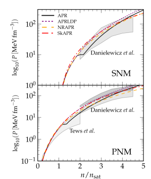
Figure 1: Pressure of SNM (top) and PNM (bottom) for the EOS’s of APR, APR_LDP, NRAPR, and SkAPR. The SNM and PNM results are compared to the pressure of nuclear matter deduced from analysis of heavy ion collision experiments by Danielewicz et al. Danielewicz, Lacey, and Lynch (2002). The PNM results are also compared to results from chiral effective field theory supplemented by piece-wise polynomials by Tews et al. Tews et al. (2018).

In Fig. 1, we show the pressures of SNM and PNM at zero temperature for each of the four EOSs: APR, APR_LDP, NRAPR, and SkAPR. The pressures as a function of density for all EOSs are mostly within the bands computed by Danielewicz et al. from analysis of collective flow in heavy ion collision experiments Danielewicz, Lacey, and Lynch (2002) and the chiral effective theory results of Tews et al. Tews et al. (2018). Note that results from microscopic calculations from the latter source are limited to about $2n_{sat}$, but are extended beyond using piece-wise polynomials that preserve causality. Quantitative differences between predictions of the different EOSs become apparent with progressively increasing density.

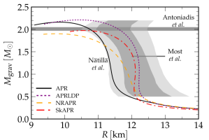
Figure 2: Mass radius relationships for the models of APR, APR_LDP, NRAPR, and SkAPR computed for charge neutral and temperature beta-equilibrated matter at zero temperature. Results are compared to the maximum NS mass observed by Antoniadis et al. J. Antoniadis et al. (2013), the mass radius relationship of Nättilä et al. Nättilä et al. (2016), and the radius of a $1.4M_{\odot}$ NS inferred by Most et al. Most et al. (2018).

Table 3: Properties of cold beta-equilibrated NSs with $M=1.4M_{\odot}$ and $M=M_{\rm max}$ for the four EOSs computed in this work, APR, APR_LDP, SkAPR, and NRAPR. The compactness $\beta=(GM_{\odot}/c^{2})(M/M_{\odot})/R$. Conversion factors used were $1\,\mathrm{MeV\,fm}^{-3}=6.242\times 10^{-34}\,\mathrm{erg\,g}^{-1}$ for the pressure and $1\,\mathrm{g\,cm}^{-3}=5.97\times 10^{-16}\,\mathrm{fm}^{-3}$ for the density.

Property	APR	APRLDP	SkAPR	NRAPR	Units
$R_{1.4}$	$11.31$	$12.18$	$12.04$	$11.58$	km
$\beta_{1.4}$	$0.18$	$0.17$	$0.17$	$0.18$
$n_{c,1.4}$	$3.46$	$2.85$	$2.98$	$3.58$	$n_{\rm sat}$
$P_{c,1.4}$	$96.2$	$67.9$	$72.1$	$94.2$	Mev fm-3
$y_{c,1.4}$	$0.089$	$0.110$	$0.094$	$0.079$
$R_{{\rm max}}$	$10.41$	$9.88$	$10.59$	$9.77$	km
$M_{{\rm max}}$	$2.162$	$2.212$	$1.974$	$1.903$	$M_{\odot}$
$\beta_{{\rm max}}$	$0.31$	$0.33$	$0.28$	$0.29$
$n_{c,{\rm max}}$	$6.63$	$7.11$	$6.79$	$7.98$	$n_{\rm sat}$
$P_{c,{\rm max}}$	$889$	$1059$	$514$	$780$	MeV fm-3
$y_{c,{\rm max}}$	$0.160$	$0.129$	$0.146$	$0.039$

The mass radius relationship of cold non-rotating neutron stars (NSs) for each EOS is shown in Fig. 2. These relations are obtained solving the TOV equations for charge neutral and beta-equilibrated matter at zero temperature Tolman (1939). For comparison the maximum NS mass observed to date, that of PSR J0348+0432 with $2.01\pm 0.04M_{\odot}$ J. Antoniadis et al. (2013) is also shown in this figure. A similar mass measurement, but for a different NS, PSR J1614-2230 with $M=1.93\pm 0.02$ Fonseca et al. (2016), boosts our confidence that NSs with at least $2M_{\odot}$ exist in nature and, thus, any realistic EOS should reproduce this limit. While APR and APR_LDP predict, respectively, maximum masses $M_{\rm max}=2.17M_{\odot}$ and $2.21M_{\odot}$, well above the $2.01\pm 0.04M_{\odot}$ limit, SkAPR barely reaches the lower limit of the observation, $M_{\rm max}=1.97M_{\odot}$, and NRAPR is two standard deviations below the lower limit, $M_{\rm max}=1.90M_{\odot}$. Properties of cold beta-equilibrated NSs are shown in Table 3. The compactness parameters $\beta=(GM_{\odot}/c^{2})(M/M_{\odot})/R$ are very nearly the same for both the $1.4M_{\odot}$ and maximum mass stars for all the EOSs listed in this table.

NS radii are less constrained than their maximum masses. From the NS merger observation GW170817 B. P. Abbott et al. (2017a, b), Most et al. predict that canonical NSs with mass $1.4M_{\odot}$ have radii in the range $12\,\mathrm{km}\leq R_{1.4}\leq 13.45\,\mathrm{km}$. In contrast, De et al. constrain radii to be in the $8.9\,\mathrm{km}<\bar{R}<13.2\,\mathrm{km}$ interval by analyzing of Love numbers from the observation of GW170817 De et al. (2018). Although we show the constraint of Most et al. in our plot for comparison between EOSs, more observations are needed to confirm their result. Note that only APR_LDP and SkAPR satisfy the constraint of Most et al. and predict, respectively, $R_{1.4}=12.2\,\mathrm{km}$ and $12.0\,\mathrm{km}$. The APR and NRAPR EOSs, on the other hand, predict radii that are too small for a canonical NS when compared to the results of Most et al., $R_{1.4}=11.2\,\mathrm{km}$ and $11.5\,\mathrm{km}$, respectively. However, all four EOSs are well within the bounds determined by De et al. De et al. (2018). Furthermore, except for the heaviest NSs in the SkAPR case, both APR_LDP and SkAPR mass-radius relationships are within $1\sigma$ range of “model A” of Nättilä et al. obtained from observations of x-ray bursts Nättilä et al. (2016) and also shown in our Fig. 2. APR (NRAPR) is within the $2\sigma$ range of the results of Nättilä et al., except for the NSs above $2.1M_{\odot}$ ($1.7M_{\odot}$).

It is worthwhile to note here that combining electromagnetic B. P. Abbott et al. (2017b) and gravitational wave information from the merger GW170817, Ref. Margalit and Metzger (2017) provides constraints on the radius $R_{\rm ns}$ and maximum gravitational mass $M_{\rm max}^{g}$ of a neutron star:

$$M_{\rm max}^{g} \lesssim 2.17M_{\odot}\,$$

$$R_{1.3} \gtrsim 3.1GM_{\rm max}^{g}\simeq 9.92~{}{\rm km}\,,$$ (26)

where $R_{1.3}$ is the radius of a 1.3$M_{\odot}$ neutron star and its numerical value above corresponds to $M_{\rm max}^{g}=2.17~{}M_{\odot}$.

III.2 Effective Masses

Nucleon effective masses for the APR and NRAPR EOSs are compared in Figs. 3 and 4. Results for SkAPR are not shown as they are very similar to those of NRAPR in that $m^{\star}$ and $\Delta m^{\star}$ are nearly the same for the two models, see Tab. 2. The effective mass contributes directly to the thermal component of the EOS, see Eq. (3). Thus, differences in effective masses contribute to differences in the thermodynamical properties of dense matter at non-zero temperatures. While differences in effective masses between APR and NRAPR below nuclear saturation density $n_{\rm sat}$ are negligible, they become significant with increasing as density. Specifically, the decrease of the effective masses for the APR model is somewhat slower than those of the NRAPR model. A similar behavior has also been observed by Constantinou et al. Constantinou et al. (2014) when comparing APR and Ska EOSs Köhler (1976); see their Fig. 1. Such differences can have consequences in astrophysical applications. As the stellar core compresses in core collapse supernovae simulations, we expect that for the same density the temperature will be larger the lower the effective mass is.

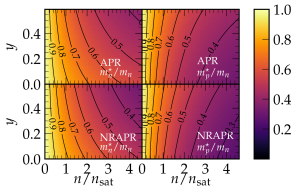
Figure 3: Neutron (left) and proton (right) effective masses $m_{t}$ normalized by the neutron vacuum mass $m_{n}$ as a function of density $n$ and proton fraction $y$ for the APR (top) and NRAPR (bottom) models.

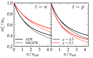
Figure 4: Neutron (left) and proton (right) effective masses for the APR (thick) and NRAPR (thin) EOSs for proton fractions $y=0.10$ (red) and $0.50$ (black).

III.3 Surface Properties of Nuclei at $T\neq 0$

Using the methods described in Appendix E, we compute surface properties of nuclei by minimizing the nuclear surface tension $\sigma^{\prime}(y_{i},T)$ between two slabs of semi-infinite matter: a dense slab with nucleon number density $n_{i}$ and proton fraction $y_{i}$, and a dilute one with density $n_{o}$ and proton fraction $y_{o}$. We determine the equilibrium configurations for a range of proton fractions $y_{i}$ in the densest phase and temperatures $T$ of the system. We then compute the parameters $\lambda$, $q$, and $p$ that define the fit $\sigma(y_{i},T)$ in Eqs. (21) and (22) by minimizing the difference between $\sigma$ and $\sigma^{\prime}$. The values of the surface tension fit parameters as well as the surface level density $A_{S}$, surface symmetry energy $S_{S}$, and the parameters of the critical temperature fit for phase coexistence $T_{c}(y)$, Eq. (140), are shown in Table 4. Note that since APR and APR_LDP only differ at densities larger than the ones of interest here their surface properties are exactly the same. For the SkAPR EOS we computed the values of the fit assuming that its $q_{tt^{\prime}}$ coefficients match those of APR for SNM at saturation density.

Table 4: Nuclear surface tension $\sigma(y_{i},T)$ fitting parameters, $\sigma_{s}$, $\lambda$, $q$, and $p$ in Eq. (21) for the EOSs of APR, NRAPR, and SkAPR. We also show the nuclear surface symmetry energy $S_{S}$, the surface level density $A_{S}$, and the parameters of the critical temperature fit $T_{c}(y)$ for phase coexistence for two semi-infinite slabs of nuclear matter.

Quantity	APR	SkAPR	NRAPR	Units
$\lambda$	$3.12$	$3.38$	$3.51$
$q$	$11.2$	$21.1$	$13.6$
$p$	$1.61$	$1.52$	$1.46$
$\sigma_{s}$	$1.20$	$1.31$	$1.14$	MeV fm-2
$A_{S}$	$0.978$	$1.30$	$1.31$	MeV fm-1
$S_{S}$	$76.8$	$79.1$	$93.0$	MeV
$T_{c0}$	$17.92$	$15.80$	$14.39$	MeV
$a_{c}$	$1.004$	$1.004$	$1.002$
$b_{c}$	$-1.025$	$-1.053$	$-1.152$
$c_{c}$	$0.697$	$0.771$	$0.470$
$d_{c}$	$-1.400$	$-1.456$	$-0.993$

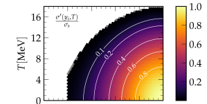
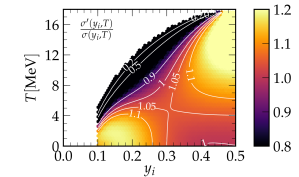
Figure 5: Surface properties $\sigma^{\prime}(y_{i},T)$ computed for the APR model (top), its best fit $\sigma(y_{i},T)$ using Eqs. (21) and (22) (center), and ratio between the computed and best fit $\sigma^{\prime}(y_{i},T)/\sigma(y_{i},T)$ (bottom). White regions are places where matter is unstable against phase coexistence.

In Fig. 5, we plot the surface tension $\sigma^{\prime}$ obtained for the EOS of APR and its best fit $\sigma$ following Eqs. (21) and (22), and the ratio between the computed properties and its best fit $\sigma^{\prime}/\sigma$. As expected, the surface tension $\sigma^{\prime}$ is largest for symmetric matter at zero temperature and decreases as matter becomes neutron rich and/or as its temperature is increased. For temperatures above the critical temperature $T_{c}=17.9\,\mathrm{MeV}$, the system is unstable against phase coexistence. For very neutron rich matter, the surface tension fit $\sigma$ goes to zero for $y_{i}=0.06$, indicating that there is no equilibrium between coexisting phases if the proton fraction of the densest phase drops below this value. However, our algorithm is unable to find solutions for $y\lesssim 0.10$ as the surface tension between the dense and dilute phases is too small and the surface extends over long distances.

The values for the surface tension $\sigma^{\prime}$ and its fit $\sigma$ agree well in most of the parameter space as seen in the top and center plots of Fig. 5. We note, however, that the ratios between $\sigma$ and $\sigma^{\prime}$ differ by 10 to 20% for symmetric matter at high temperatures and for neutron rich matter at temperatures below $\sim 3\,\mathrm{MeV}$. Furthermore, for regions of the $y_{i}$-$T$ phase space where $\sigma^{\prime}/\sigma_{s}$ is below 0.3, the fitting function $\sigma$ overestimates the surface tension $\sigma^{\prime}$ by as much as a factor of 5. Thus, a different fitting function may be needed in order to accurately probe this region. We defer this to future work.

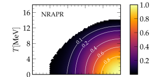
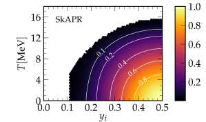
Figure 6: Plots of normalized surface tension $\sigma(y_{i},T)/\sigma_{s}$ for APR (top), NRAPR (center), and SkAPR (bottom) EOSs. White regions indicate areas of the parameter space where there is no coexistence of matter with two different densities and proton fractions.

In Fig. 6, we plot the surface tension fit $\sigma(y_{i},T)$ for the APR, NRAPR and SkAPR models. All three EOSs have the same qualitative behavior for $\sigma(y_{i},T)$. We notice that the APR model predicts coexistence of dense and dilute phases for symmetric nuclear matter for temperatures higher than the other two EOSs. The values of the critical temperatures for each EOS are presented in Tab. 4. As for the APR model, our algorithm to obtain $\sigma^{\prime}$ fails to obtain coexisting phases for proton fractions lower than $y_{i}=0.10$ for NRAPR and SkAPR. However, we do not expect this failure to significantly alter the parameters of the fit function $\sigma$.

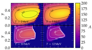
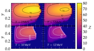
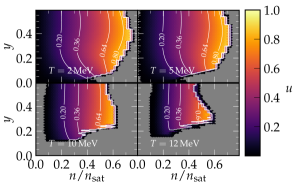
Figure 7: Nuclear mass number $A$, charge $Z$ and the volume fraction $u$ occupied by the dense phase for the APR model.

Once the surface properties have been determined, we focus our attention of the subnuclear density region $0.1\lesssim n/n_{\rm sat}\lesssim 0.8$ of parameter space with temperatures lower than $T_{c}(y)$, i.e., where the nuclear pasta is expected to occur. In Figs. 7, 8, and 9 we plot, respectively, the nuclear mass number $A$, its charge $Z$ as well as the volume fraction $u$ occupied by the dense phase in each Wigner-Seitz cell for the APR, NRAPR, and SkAPR models. Results shown are for four temperatures, $T=2,\,5,\,10,\,12\,\mathrm{MeV}$.

Within the formalism used, the volume fraction $u$ is directly related to the topological phase of nuclear matter. Following the procedure of Lattimer & Swesty Lattimer and Swesty (1991) and detailed in Fig. 4 of Lim & Holt Lim and Holt (2017), the occupied volume fraction of the dense phase describes (1) spherical nuclei for $u<0.20$, (2) cylindrical nuclei for $0.20\leq u<0.36$, (3) flat sheets for $0.36\leq u<0.64$, (4) cylindrical holes for $0.64\leq u<0.80$, and (5) spherical holes for $u\geq 0.80$. In the Figs. 7, 8, and 9, the gray area represents regions where nuclear matter is in a uniform phase.

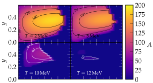
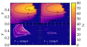
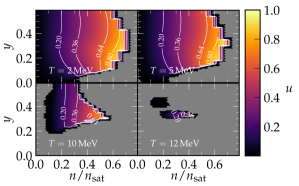
Figure 8: Same as Fig. 7, but for the NRAPR model.

We note that SkAPR and APR produce nuclei with larger mass numbers than NRAPR owing to their higher compression moduli, $K_{\rm sat}=266\,\mathrm{MeV}$ compared to $K_{\rm sat}=226\,\mathrm{MeV}$ of NRAPR. As expected from the surface tension plot, Fig. 6, the APR model predicts nuclei that perist up to higher temperatures than for the Skyrme EOSs. This is likely due to the density dependence of the $q_{tt^{\prime}}$ in the APR model, see Eqs. (25), which is absent in the Skyrme model.

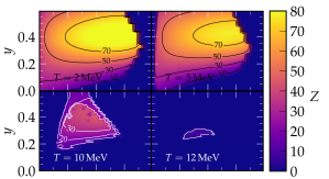
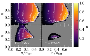
Figure 9: Same as Fig. 7, but for the SkAPR model.

As the temperature increases, uniform nuclear matter occupies larger and larger fraction of the $y-n$ parameter space. In all cases, spherical holes seem to disappear first followed by cylindrical holes. The last region to disappear for all EOSs (not shown for APR), is for proton fractions $0.2\lesssim y\lesssim 0.4$ at densities $0.2\lesssim n/n_{\rm sat}\lesssim 0.4$. This happens even though the surface tension is larger for SNM than for neutron rich matter. Similar results, albeit with small quantitative differences, are obtained in other works which use SNA near the transition to uniform nuclear matter Lattimer and Swesty (1991); Shen et al. (1998); Shen, Horowitz, and Teige (2011). Relaxing the assumptions made therein to compute the free energy near the transition region, so that SNM melts at a higher temperature than neutron rich matter, will be taken up in future work.

III.4 Composition of the System at $T\neq 0$

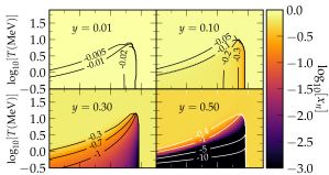
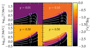
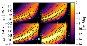
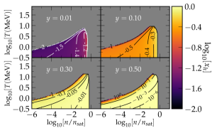
Figure 10: From top to bottom: number fraction of neutrons $x_{n}$, protons $x_{p}$, alpha particles $x_{\alpha}$, and heavy nuclei $x_{h}$ for proton fraction $y=0.01,\,0.10,\,0.30$ and $0.50$ for the APR EOS.

In Fig. 10, we display the composition of the system for the APR model. We plot neutron, proton, alpha particle, and heavy nuclei number fractions $x_{n}$, $x_{p}$, $x_{\alpha}$, and $x_{h}$, respectively. The qualitative behavior of the composition for the other EOSs is the same as for the APR EOS across all of parameter space. However, there are minor quantitative differences between the APR and the Skyrme EOSs, as for example, APR predicts that heavy nuclei melt at higher temperatures, especially at densities close to the nuclear saturation density.

We note that all expected qualitative behavior for the EOSs are fulfilled. For SNM at densities $n\lesssim 0.10\,\mathrm{fm}^{-3}$ and temperatures $T\lesssim 1\,\mathrm{MeV}$, most nucleons cluster into heavy nuclei, a few into alpha particles whereas a very small fraction is free due to temperature effects. As density increases and reaches $n\simeq 0.10\,\mathrm{fm}^{-3}$ nucleons occupy all the space available to them and matter becomes uniform. As temperature is increased, heavy nuclei progressively breakup into alpha particles until at even alpha particles start to breakup and the system is driven closer to a uniform free nucleon gas. If, instead, proton fraction is decreased, neutrons drift out of heavy nuclei, alpha particles breakup, and the system as a whole becomes neutron rich.

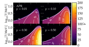
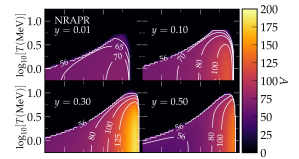
Figure 11: From top to bottom: sizes of nuclei for the APR (top), NRAPR (center), SkAPR (bottom) EOSs for proton fraction $y=0.01,\,0.10,\,0.30$ and $0.50$.

In Fig. 11 we plot the mass numbers of nuclei for the different EOSs in the temperature and density plane. As was shown in Figs. 7, 8, and 9, the SkAPR EOS predicts the most massive nuclei, while APR often predicts higher melting temperatures for heavy nuclei and that nuclei survive up to larger isospin asymmetries. The black area represents regions where nuclear matter is in a uniform phase.

III.5 High Density Phase Transition in APR

The EOSs of AP, and thus APR, predicts that at high densities there is a phase transition from pure nucleonic matter to a phase that includes nucleons and a neutral pion condensation. In the APR formalism, this phase transition is taken into account by including extra potential terms in the high density phase (HDP) compared to the low density phase (LDP), see Eqs. (12) and (13). The extra terms in the HDP soften the EOS at high densities and cause a discontinuity in the pressure and chemical potentials of the EOS of APR. In a self-consistent EOS for astrophysical simulations there must be no pressure discontinuities as well as no points where $dP/dn|_{T}<0$. To avoid such regions, we perform a Maxwell construction in the manner described in Sec. VI of Ref. Constantinou et al. (2014). This results in a mixed phase for densities near $n\sim n_{\rm tr}(y)$, see Eq. (5).

In Fig. 12, we compare the pressure per baryon $P/n$ of the APR EOS with its variant that only includes the stiffer LDP, APR_LDP. In regions of phase space near $n\simeq 1.3n_{\rm sat}$ for almost PNM, $y=0.01$, to $n\simeq 2n_{\rm sat}$ for SNM, $y=0.50$, the pressure per baryon remains constant as the baryon number density of the system increases at constant temperature. This is the region where our Maxwell construction finds a mixed phase of LDP and HDP, see also Fig. 32 of Constantinou et al. Constantinou et al. (2014) for how the mixed phase changes with proton fraction and temperature. Notice that no such region exists for the APR_LDP EOS and the pressure.

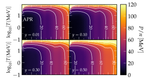
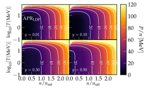
Figure 12: Pressure per baryon $P/n$ for APR EOS (top) and APRLDP (bottom) for proton fraction $y=0.01,\,0.10,\,0.30$ and $0.50$.

We show the chemical potential splitting $\hat{\mu}=\mu_{n}-\mu_{p}$ in Fig. 13. Comparing the EOSs of APR and APR_LDP, we observe that $\hat{\mu}$ exhibits a sharp drop of about $1$ to $2\,\mathrm{MeV}$ in the mixed phase region.

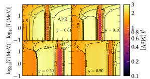
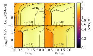
Figure 13: Chemical potential splitting $\hat{\mu}=\mu_{n}-\mu_{p}$ for APR EOS (top) and APRLDP (bottom) for proton fraction $y=0.01,\,0.10,\,0.30$ and $0.50$.

IV Core-collapse Supernovae

We have carried out a set of example core-collapse and post bounce core-collapse supernovae (CCSNe) simulations in spherical symmetry. We investigated how the new APR EOSs compare to the Skyrme EOSs in this important astrophysical scenario and discuss the influence of the EOS on core-collapse post bounce evolution and black hole formation. For these simulations, the EOS for the low density phase below $10^{-3}~{}{\rm fm}^{-3}$ used was that of 3,335 nuclei in NSE. The match between the NSE and the single nucleus approximation (SNA) EOSs was performed using the simple merge function described in Sec. VII of SRO Schneider, Roberts, and Ott (2017) with the parameters $n_{t}=10^{-3}\,\mathrm{fm}^{-3}$ and $n_{\delta}=0.33$.

The CCSNe simulations were performed employing the open-source spherically-symmetric (1D) general-relativistic hydrodynamics code GR1D O’Connor and Ott (2010, 2011, 2013); O’Connor (2015). Unlike in the SRO paper, we treat neutrino transport using the two-moment neutrino transport solver. This is achieved using the NuLib neutrino transport library which builds a database of energy dependent multi-species M1 neutrino transport properties O’Connor (2015). We consider three neutrino species: $\nu_{e}$, $\nu_{\bar{e}}$, and $\nu_{x}=\nu_{\mu}=\nu_{\bar{\mu}}=\nu_{\tau}=\nu_{\bar{\tau}}$. The energy grid for each neutrino type has 24 logarithmically spaced groups. The first group is centered at 1$\,\mathrm{MeV}$ and has a width of 2$\,\mathrm{MeV}$. The last group is centered at $\sim 269\,\mathrm{MeV}$ and has a width of $\sim 35\,\mathrm{MeV}$.

We simulated the core-collapse and post bounce evolution of two progenitors: (1) a 15$M_{\odot}$ progenitor of Woosley, Heger, and Weaver Woosley, Heger, and Weaver (2002) and (2) a 40$M_{\odot}$ progenitor of Woosley and Heger Woosley and Heger (2007). While the former is expected to explode as a SN, at least in multi dimensional simulations, and leave a neutron star remnant the latter is very massive and has a high-compactness which favors black hole (BH) formation O’Connor and Ott (2011). For both progenitors we used a computational grid with $1\,500$ grid cells, constant cell size of $100\,\mathrm{m}$ out to a radius of $20\,\mathrm{km}$, and then geometrically increasing cell size to an outer radius of $10\,000\,\mathrm{km}$.

Stellar evolution codes, such as the ones that generate the two progenitors in our simulations, use reaction networks and, thus, the pre-collapse relationship between thermodynamical variables can differ substantially from the ones in the EOSs used in CCSN simulations. To start our simulations in a way that is as consistent as possible with the hydrodynamical structure of the progenitor models, we map the stellar rest-mass density $\rho$, proton fraction $y$, and pressure $P$ to GR1D, and then find the temperature $T$, specific internal energy $\epsilon$, entropy $s$, etc., using our EOS tables. This approach for setting up the initial conditions results in differences between the original stellar profile and the GR1D initial conditions in all quantities except $\rho$, $y$, and $P$. This treatment differs from most CCSNe simulations which match $\rho$, $y$, and $T$ between pre-supernova progenitors and the core-collapse simulation.

IV.0.1 15$M_{\odot}$ Progenitor

We followed the collapse and post-bounce evolution of the $15M_{\odot}$ progenitor up to $1.0\,\mathrm{s}$ after bounce. Stars with such mass are expected to explode in nature and do so in some multi dimensional simulations Yakunin et al. (2010); Ott et al. (2018), albeit for different pre-supernova progenitor models Woosley and Weaver (1995); Woosley and Heger (2007). However, we do not observe explosions in our GR1D simulations, which is consistent with other 1D simulations for this progenitor O’Connor and Ott (2010).

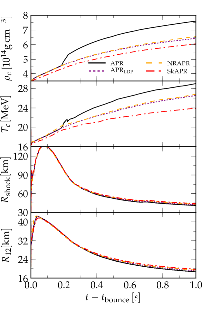
Figure 14: (Color online) From top to bottom: central density $\rho_{c}$, central temperature $T_{c}$, shock radius $R_{\rm{shock}}$, and PNS radius $R_{12}$ for the core-collapse of the $15\,M_{\odot}$ pre-supernova progenitor of Woosley, Heger, and Weaver Woosley, Heger, and Weaver (2002).

In Fig. 14, we plot the central density and temperature temperature as a function of time after bounce $t_{\rm bounce}=0.351\,\mathrm{s}$ as well as the shock radius and neutron star (NS) radius defined as the radius where the density is $\rho=10^{12}\,\mathrm{g\,cm}^{-3}$. We observe significant differences in the core density $\rho_{c}$ and its temperature $T_{c}$ between the APR EOS and its version APR_LDP without the high density transition. Also, results for the NRAPR EOS of Steiner et al. Steiner et al. (2005) agree better with those obtained using the APR_LDP EOS than those from the SkAPR EOS. This happens even though the properties of SkAPR near saturation density match more closely those of APR_LDP than NRAPR does, see Tab. 2, implying there is a trade-off between the different approaches to the EOS and exactly matching their observables.

We see a shift in both the density and temperature at the core of the PNS once the core density is above the region where the pion condensate appears according to the EOS model. However, the outer regions of the PNS and the shock front are only weakly affected by the phase transition. Although the PNS and shock radius contract faster due to the high density transition, this change is only of order a few %. Furthermore, for this model and the APR EOS, we do not see a second spike in the neutrino signal triggered by the phase transition, as reported by Sagert et al. for the case a hadron-to-quark matter phase transition Sagert et al. (2009), see Fig. 15.

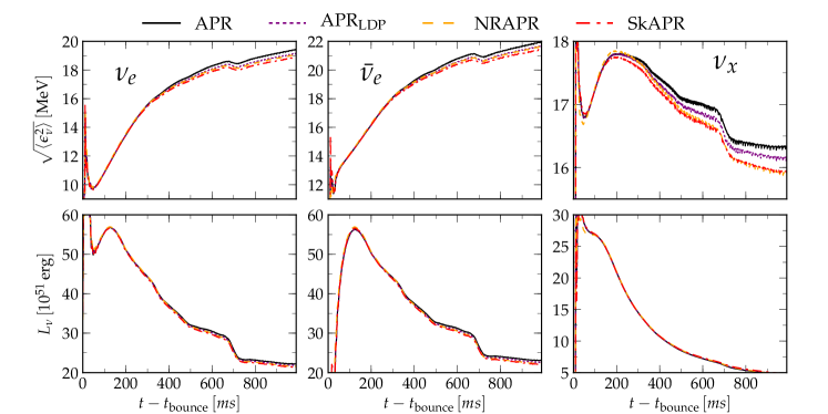
Figure 15: (Color online) Root mean square energy $\sqrt{\langle\epsilon^{2}_{\nu}\rangle}$ (top) and luminosity $L_{\nu}$ (bottom) for electron neutrinos $\nu_{e}$ (left), electron anti-neutrinos $\nu_{\bar{e}}$ (center), and one of heavy neutrinos $\nu_{x}$ (right) for the core-collapse of the $15\,M_{\odot}$ pre-supernova progenitor of Woosley, Heger, and Weaver Woosley, Heger, and Weaver (2002). The results for the heavy neutrinos $\nu_{x}$ have been divided by 4 as it includes four neutrino types. We have added $2\times 10^{52}\,\mathrm{erg}$ to the luminosity $L_{\nu_{x}}$ so that it fits with the same scale as the luminosity for the other two species.

The neutrino spectra, root mean square $\sqrt{\langle\epsilon^{2}_{\nu}\rangle}$ and luminosity $L_{\nu}$, for the different neutrino species are shown in Fig. 15. We note that at the time the core densities are large enough that there is a phase transition in the APR EOS, there is a short contraction in the PNS and shock radii. This contraction heats up slightly the neutrino-sphere and increases the energy and luminosity of neutrinos emitted. Nevertheless, this change is only of a few % and of the same order as changes seen between the two different Skyrme EOSs, NRAPR and SkAPR, for which observables such as the incompressibility $K_{\rm sat}$ changed by a large amount.

IV.0.2 40$M_{\odot}$ Progenitor

We now follow the core-collapse and post-bounce evolution of the $40M_{\odot}$ progenitor of Woosley and Heger Woosley and Heger (2007) until a black hole (BH) forms. This progenitor is one of the many studied by O’Connor and Ott O’Connor and Ott (2011) using a neutrino leakage scheme transport and four different EOSs, the three Lattimer and Swesty (LS) variants Lattimer and Swesty (1991) and the Shen EOS with the TM1 parametrization Shen et al. (1998). O’Connor and Ott observed that larger incompressibilities lead to a faster collapse to BH, although effects of the effective mass, which are important for the temperature dependence of the EOS Steiner, Hempel, and Fischer (2013); Constantinou et al. (2014); Schneider et al. , on the different BH formation time and its initial mass were not disentangled. The three LS EOSs, with incompressibility $K_{\rm sat}=180$, $220$, and $375\,\mathrm{MeV}$ all have effective masses set to the nucleon vacuum mass. The Shen TM1 EOS has $K_{\rm sat}=280\,\mathrm{MeV}$ and predicts an effective mass for symmetric nuclear matter at nuclear saturation density $m^{\star}=0.63m_{n}$. All else being equal for the zero temperature properties of nuclear matter, a lower effective mass will lead to higher thermal pressure and a slower collapse to BH Schneider et al. .

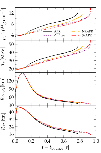
Figure 16: (Color online). Same as Fig. 14, but for the 40$M_{\odot}$ pre-supernova progenitor of Wooseley and Heger Woosley and Heger (2007).

In the four EOSs studied here, the effective masses all have very similar values at the saturation density, see Tab. 2. However, the effective masses for the Skyrme EOSs decrease faster at higher densities than for the APR EOSs, Fig. 3. Other main differences between these EOSs are the lower incompressibility $K_{\rm sat}$ for NRAPR and the high density transition in APR. Thus, we expect that using the APR EOS will lead to a faster collapse to BH than for the other EOSs, due to the sharp phase transition discussed in Sec. II. This is indeed the case as seen in Fig. 16. We also expect the NRAPR EOS to predict a faster collapse than SkAPR and APR_LDP due to its lower incompressibility $K_{\rm sat}$. This feature is also observed. However, it is difficult to predict which of SkAPR or APR_LDP will take the longest to collapse. This is due to a possible trade-off between the slightly higher (lower) pressures for the SkAPR EOS than for the APR_LDP EOS for $n\lesssim 2n_{\rm sat}$ ($n\gtrsim 2n_{\rm sat}$) and its lower nucleon effective masses at densities $n\gtrsim 2n_{\rm sat}$. In fact, what we observe is that near $500\,\mathrm{ms}$ after bounce SkAPR EOS predicts lower densities and temperatures at the core of the PNS than the APR_LDP EOS. At that time, the density at the core is approximately $2.5n_{\rm sat}$, a region where the effective mass for the SkAPR EOS has deviated from its APR_LDP counterpart. From then on the core temperature computed with the SkAPR is slightly higher than that for the APR_LDP EOS. However, in the same region the pressure obtained with the APR_LDP EOS is slightly higher. The competition between both effects leads to both EOSs predicting an almost identical collapse time to BH, Tab. 5. We also see, as observed by O’Connor and Ott, that there is a correlation between the time to collapse into a BH and its initial mass. This is due to the accretion rate being only dependent on the low density part of the EOS, which was set as the same for all four EOSs.

Table 5: Black hole formation times and their gravitational mass at the time of collapse. The time to bounce for all EOSs is $t_{\rm{bounce}}=0.472\,\mathrm{s}$.

EOS	$t_{\rm{BH}}-t_{\rm{bounce}}$	$t_{\rm{BH}}$	$M_{\rm{grav}}\,[M_{\odot}]$
APR	1.252	0.780	2.580
NRAPR	1.304	0.832	2.611
APRLDP	1.403	0.931	2.670
SkAPR	1.405	0.933	2.672

As for the $15\,M_{\odot}$ case, differences in the inner regions of the PNS do not lead to significant changes in either shock or the PNS radius, bottom panels of Fig. 17. However, both neutrino energies and luminosities, especially for heavy $\nu_{x}$ neutrinos, are enhanced for the EOSs that predict faster collapse to BH, Fig. 17. Another feature of the neutrino spectrum is the sharp decrease in the luminosity for all four EOSs and neutrino species near $400\,\mathrm{ms}$ after bounce. This is due to the rapid change in the accretion rate as the density discontinuity of the Si/Si-O shell of the star passes the stalled shock front, see Fig. 4 of O’Connor and Ott O’Connor and Ott (2011). For 3D simulations, Ott et al. have shown that the high neutrino luminosities and energies lead to a shock explosion even before the Si/Si-O shell crosses the shock radius Ott et al. (2018), although the hot PNS left behind is massive enough that it will subside into a BH once it cools down. Unlike for the lower mass progenitor studied here, the neutrino luminosities show significant differences at late times due to the phase transition present in the APR EOS. Thus, it is likely that in multi-dimensional simulations the phase transition in the APR EOS leads to faster shock revival and expansion. Such a future study is indicated by results of this work.

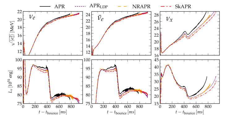
Figure 17: (Color online) Root mean square energy $\sqrt{\langle\epsilon^{2}_{\nu}\rangle}$ (top) and luminosity $L_{\nu}$ (bottom) for electron neutrinos $\nu_{e}$ (left), electron anti-neutrinos $\nu_{\bar{e}}$ (center), and one of heavy neutrinos $\nu_{x}$ (right) for the core-collapse of the $40\,M_{\odot}$ pre-supernova progenitor of Woosley and Heger Woosley and Heger (2007). The results for the heavy neutrinos $\nu_{x}$ have been divided by 4 as it includes four neutrino types. We have added $6\times 10^{52}\,\mathrm{erg}$ to the luminosity $L_{\nu_{x}}$ so that it fits with the same scale as the luminosity for the other two species.

V Summary and Conclusions

Our primary objective in this work has been to build an equation of state (EOS) for simulations of supernovae, neutron stars and binary mergers based on the Akmanl, Pandharipand and Ravenhall (APR) Hamiltonian density devised to reproduce the results of the microscopic potential model calculations of Akmal and Pandharipande (AP) for nucleonic matter with varying isospin asymmetry. Toward this end, we have developed a code that takes advantage of the structure of the SRO EOS code which was devised to compute EOSs for Skyrme parametrizations of the nuclear force Schneider, Roberts, and Ott (2017). Here, the SRO EOS code was adapted to compute EOSs using the more intricate APR potentials Akmal, Pandharipande, and Ravenhall (1998). The APR potential has some distinct differences compared to Skyrme-type potentials. Skyrme parameters are fit to reproduce properties of finite nuclei or empirical parameters of the expansion of energy density of nuclear matter around saturation density. In contrast, APR has been fit to reproduce results of variational calculations based on a microscopic potential model for both symmetric nuclear matter (SNM) and pure neutron matter (PNM). These variational calculations include two- and three-body interactions as well as relativistic boost corrections. Furthermore, APR contains a phase transition to a neutral pion condensate that softens the EOS at high densities while still predicting cold beta-equilibrated neutron star (NS) masses and radii in agreement with current observations J. Antoniadis et al. (2013); Fonseca et al. (2016); Most et al. (2018); Nättilä et al. (2016); De et al. (2018).

In addition to the APR EOS, we have developed three other EOSs: (1) APR_LDP, an APR variant which does not include a transition to a neutral pion condensate at high densities, (2) a finite temperature version of the non-relativistic APR model of Steiner et al., NRAPR Steiner et al. (2005); Schneider, Roberts, and Ott (2017), and (3) SkAPR Schneider et al. ; Margueron, Hoffmann Casali, and Gulminelli (2018), a Skyrme-type version of APR computed with the SRO code which was fit to reproduce some of the properties.

In our calculations of the EOS of APR, we pay special attention to the surface properties of nuclear matter and its inhomogeneous phases. The APR model allows for more complex behavior of the effective masses of nucleons when compared to Skyrme EOSs. In addition, it allows for asymmetries between neutron-neutron and proton-proton gradient terms in the surface component of the Hamiltonian which is generally not present in the commonly used Skyrme EOSs. This allows the APR EOS to predict non-uniform nuclear matter up to higher densities, temperatures, and lower proton fractions than the Skyrme-type EOSs allow.

Using the above four EOSs, we simulated spherically symmetric core-collapse of two massive stars, a $15M_{\odot}$ pre-supernova progenitor Woosley, Heger, and Weaver (2002) and a $40M_{\odot}$ pre-supernova progenitor Woosley and Heger (2007). We followed the evolution of the $15M_{\odot}$ progenitor for one second after core-bounce and the formation of a proton NS (PNS). Although there are some significant differences observed across EOSs for the inner configuration of the star, neither the outer regions of the collapsing star nor the neutrino spectra seem to be significantly affected by either the phase transition included in the APR EOS or by the Skyrme or APR description of the EOS. Besides the development of a new EOS, one of our main goals was to determine whether the phase transition that includes a high density neutral pion condensate alters the neutrino spectrum of a collapsing star and leads to a second peak in neutrino signal, as observed by Sagert et al. for the hadron-to-quark phase transition Sagert et al. (2009). Note that one of the progenitors in Ref. Sagert et al. (2009) is the same as the $15\,M_{\odot}$ pre-supernova progenitor used here. However, we do not observe a second burst in neutrino luminosity and root mean square energy in our simulation with the APR EOS. This difference between our result and that of Sagert et al. is attributed to the lack of a second shock wave traveling through the PNS that results from the transition from hadron-to-quark matter in Sagert et al.. The softening in the APR EOS due to the existence of a pion condensate is not as extreme as that of a transition from hadron-to-quark matter and, thus, no second shock wave forms and thus second peak in the neutrino signal is not observed. We recall that the phase transition in the APR EOS as treated in Constantinou et al. (2014) is almost independent of temperature. Therefore, it is likely that the addition of a temperature dependent phase transition facilitates the formation of a second shock wave due to the large temperatures achieved in the inner regions of the PNS and due to the low proton fractions and even higher temperatures that exist in the PNS mantle.

The $40M_{\odot}$ progenitor evolution was followed until black hole (BH) formation. In this case, the differences across EOSs affect the BH formation time and its initial mass. Particularly, the softening of the APR EOS due to its prediction of a neutral pion condensate at high densities facilitates the contraction of the PNS and, thus, speeds up the NS subsidence into a BH as well as lowers its initial mass and hardens the neutrino spectrum, especially for the heavier neutrinos. The other three EOSs predict similar evolutions and neutrino spectra until a BH forms, which happens earlier for NRAPR as it is the softest EOS at high densities. We expect differences between the EOSs to be amplified in multi-dimensional simulations.

Directions for future work suggested by the first stage of the development of the EOS of APR performed here include (1) incorporating extensions of the excluded volume approach that includes ${}^{2}\rm{H},^{3}{\rm H}$ and ${}^{3}{\rm He}$ in addition $\alpha$-particles as in Ref. Lalit et al. (2018), (2) exploring consequences for PNS evolution and (3) performing simulations of binary mergers of neutron stars. More than in the evolutions of core-collapse supernovae and proto-neutron stars, the evolution of the compact object following the merger is influenced by the dense matter EOS. This is because higher densities and temperatures are achieved in the post-merger remnant than in the case of a SN or a PNS. The possible outcomes for the compact object include a massive stable neutron star, a hyper massive neutron star that can collapse to a black hole owing to deleptonization through loss of trapped neutrinos and rigidization of rotation, or, a prompt black hole. Future generation gravity wave detectors can inform on the possible outcomes from post-merger signals. For the post-merger evolution, time evolving effects of rotation, magnetic fields and temperature also become crucially important.

Appendix A Equilibrium conditions

For the most part, we follow the scheme outlined by Lattimer and Swesty (LS) Lattimer and Swesty (1991) to determine the set of equations that determines equilibrium between nucleons, electrons, positrons and photons. Departures from the LS approach will be noted as the discussion proceeds. Depending on the density, temperature and net electron fraction, nucleons can cluster into alpha particles (proxy for light nuclei) and into heavy nuclei, both of which are treated using an excluded volume approach. The total free energy of the system is

$$F=F_{o}+F_{\alpha}+F_{h}+F_{e}+F_{\gamma}\,.$$ (27)

Terms on the right hand side above are the free energies of unbound nucleons outside of alpha particles and heavy nuclei, alpha particles, heavy nuclei, leptons, and photons, respectively. Leptons and photons are treated as non-interacting relativistic uniform gases. Their free energies and thermodynamic properties are standard, and computed using the Timmes and Arnett equation of state (EOS) Timmes and Arnett (1999). The system as a whole is in thermal equilibrium at a temperature $T$ and electrically neutral, i.e., the lepton density $n_{e^{-}}-n_{e^{+}}$ and the proton density $n_{p}=ny$ ($n$ is the total baryon density and $y$ is the proton fraction) are related by $n_{p}=n_{e^{+}}-n_{e^{-}}$.

Because leptons and photons are assumed to form a uniform background and are non-interacting, their free energies do not interfere with the overall state of nucleons inside and out of nuclei. Thus, for a given nucleon number density $n$, proton fraction $y$, and temperature $T$ we compute the properties of nucleons that minimizes the free energy of the system. Two types of system are possible: (1) uniform matter, which refers to a liquid of nucleons and alpha particles, and (2) non-uniform matter, which includes heavy nuclei. The system is assumed uniform unless its temperature is lower than the critical temperature $T\lesssim T_{c}$, and nucleon density lower than nuclear saturation density, $n<n_{\rm sat}\simeq 0.16\,\mathrm{fm}^{-3}$. In the latter cases, we solve for both uniform and non-uniform matter. If only one type of matter minimizes the free energy of the system, then that is set as its true solution. However, if both solutions are possible, then we set the true state of the system as the one with the lowest free energy. We update often the possibility of finding non-uniform matter based on previously found solutions.

In Appendices C to G, we discuss the different terms in Eq. (27). Appendix H contains a description how to compute the solution for uniform matter. Appendix I describes how the solution to non-uniform matter is obtained.

Appendix B Derivative notations

To simplify the notation used throughout the Appendices, we define the density derivatives of functions $F\equiv F(n_{n},n_{p},T)$ with respect to a nucleon density $n_{t}$ keeping $n_{-t}$ fixed as

$$\partial_{n_{t}}F=\left.\frac{\partial F(n_{n},n_{p},T)}{\partial n_{t}}\right|_{n_{-t},T}\,.$$ (28)

Note that if $t=n$, then $-t=p$ and vice versa. We often interchangeably use $F(n_{n},n_{p})=F(n,y)$ making the replacements $n_{n}=(1-y)n$ and $n_{p}=yn$ where the number density is $n=n_{n}+n_{p}$ and the proton fraction $y=n_{p}/n$. In similar fashion, second derivatives are denoted by

$$\partial_{n_{r}n_{t}}F=\left.\frac{\partial^{2}F(n_{n},n_{p})}{\partial n_{t}\partial n_{r}}\right|_{n_{-t},n_{-r}}\,.$$ (29)

If $F^{\prime}\equiv F^{\prime}(\eta_{n},\eta_{p},T)$, the derivatives with respect to the degeneracy parameters $\eta_{t}$ are denoted by

$$\partial_{\eta_{t}}F^{\prime}=\left.\frac{\partial F^{\prime}(\eta_{n},\eta_{p},T)}{\partial\eta_{t}}\right|_{\eta_{-t},T}\,.$$ (30)

Whenever we take a temperature derivative and choose to keep the degeneracy parameters constant instead of the nucleon densities, we add a prime to the $\partial$ sign, i.e.,

$$\partial^{\prime}_{T}F^{\prime}=\left.\frac{\partial F^{\prime}(\eta_{t},\eta_{p},T)}{\partial T}\right|_{\eta_{n},\eta_{p}}\,.$$ (31)

We also switch between derivatives where a set of variables such as $\xi=(n_{n},n_{p},T)$ or $\xi^{\prime}=(\eta_{n},\eta_{p},T)$ is used to derivatives with respect to the independent variables $\zeta=(n,y,T)$. In the latter case, the transformation between derivatives is

$$d_{T}F =\partial_{T}F+\sum_{r}(\partial_{n_{r}}F)(\partial_{T}n_{r})\,,$$ (32a)

$$d_{n}F =\sum_{r}(\partial_{n_{r}}F)(\partial_{n}n_{r})\,,$$ (32b)

$$d_{y}F =\sum_{r}(\partial_{n_{r}}F)(\partial_{y}n_{r})\,,$$ (32c)

for $F=F(\xi)$ and

$$d_{T}F^{\prime} =\partial^{\prime}_{T}F^{\prime}+\sum_{r}(\partial_{\eta_{r}}F)(\partial_{T}\eta_{r})\,,$$ (33a)

$$d_{n}F^{\prime} =\sum_{r}(\partial_{\eta_{r}}F)(\partial_{n}\eta_{r})\,,$$ (33b)

$$d_{y}F^{\prime} =\sum_{r}(\partial_{\eta_{r}}F)(\partial_{y}\eta_{r})\,.$$ (33c)

for $F^{\prime}=F^{\prime}(\xi^{\prime})$. Above

$$d_{T}F=\left.\frac{dF}{dT}\right|_{n,y}$$ (34)

and similarly for $F^{\prime}$ and permutations of $T$, $n$, and $y$. We further define the derivative

$$d^{\prime}_{T}F=\left.\frac{dF}{dT}\right|_{n,y,\zeta^{\prime}}\,,$$ (35)

where $\zeta^{\prime}$ is a set of internal variables of the system. This will be useful when changing from derivatives with respect to $\zeta^{\prime}$ to derivatives with respect to $\xi$.

Appendix C The APR model

In this Appendix, we collect various formulas and numerical notes employed in the development of the EOS of APR.

C.1 The free energy of nucleons

The free energy of a uniform system of nucleons is computed from the thermodynamical relation

$$F_{\rm bulk}=E_{\rm bulk}-TS_{\rm bulk}\,.$$ (36)

For a given density $n$, proton fraction $y$, and temperature $T$, the internal energy $E_{\rm bulk}$ is computed from Eq. (3), $U_{\rm bulk}\rightarrow\mathcal{H}(n,y,T)$. $E_{\rm bulk}$ depends on the kinetic energy densities $\tau_{t}$, effective masses $m_{t}^{\star}$, and the APR potential $\mathcal{U}(n,y)$. The entropy $S_{\rm bulk}$ has the form

$$S_{\rm bulk}=\sum_{t}\left[\frac{5}{3}\frac{\hbar^{2}\tau_{t}}{2m^{\star}_{t}T}-Tn_{t}\eta_{t}\right]\,.$$ (37)

Note that the entropy depends also on the degeneracy parameters of nucleons $\eta_{t}$ discussed in Eq. (8) in Sec. II.1. These expressions enable the determination of the free energies of unbound nucleons in uniform matter as well as those of bound and unbound nucleons in non-uniform matter.

In what follows, we use capital letters for quantities per volume and lower case letters for specific (per baryon or per mass) quantities. Thus, the specific free energy of the nucleon system $a$ is related to its internal free energy density by $f_{a}=F_{a}/n_{a}$. Here $a=i$ stands for nucleons bound inside heavy nuclei, and $a=o$ for unbound nucleons outside heavy nuclei. Similarly, the specific entropy is written as $s_{a}=S_{a}/n_{a}$ and the specific internal energy as $\epsilon_{a}=E_{a}/n_{a}$.

C.2 The nuclear potential

We now turn our attention the the nucleon-nucleon potential in the APR model given by

$$\mathcal{U}(n,y)=g_{1}(n)\left[1-\delta^{2}(y)\right]+g_{2}(n)\delta^{2}(y)\,,$$ (38)

which may also be written in the form

$$\mathcal{U}(n_{n},n_{p})=4\frac{g_{1}}{n^{2}}n_{t}n_{-t}+\frac{g_{2}}{n^{2}}\left(n_{t}-n_{-t}\right)^{2}\,.$$ (39)

Unless otherwise explicit, we omit the functional dependences after they have been shown once. In order to simplify expressions throughout, we define the auxiliary functions

$$\phi_{i,j}=p_{i}+p_{j}n,\quad\psi_{i}=n-p_{i},\quad\kappa_{i}=e^{-p_{i}^{2}n^{2}}\,.$$ (40)

Primes are used to denote total derivatives with respect to the total nucleon number density $n$; thus,

$$\kappa^{\prime}_{i}=-2p_{i}^{2}n\kappa_{i},\quad\kappa^{\prime\prime}_{i}=\kappa^{\prime}_{i}\left[\frac{1}{n}+\frac{\kappa^{\prime}_{i}}{\kappa_{i}}\right]\,.$$ (41)

For the low density phase (LDP), i.e., for densities below those for which a neutral pion condensate forms,

$$\mathcal{U}\rightarrow\mathcal{U}_{L}=g_{1L}\left[1-\delta^{2}\right]+g_{2L}\delta^{2}\,.$$ (42)

The functions $g_{iL}$ are given by

$$g_{1L} =-n^{2}\left[p_{1}+n\phi_{2,6}+\phi_{10,11}\kappa_{9}\right]$$ (43a)

$$g_{2L} =-n^{2}\left[\frac{p_{12}}{n}+\phi_{7,8}+p_{13}\kappa_{9}\right].$$ (43b)

In the high density phase (HDP), $\mathcal{U}\rightarrow\mathcal{U}_{H}$, and $g_{iH}$ are related to $g_{iL}$ by

$$g_{1H} =g_{1L}-n^{2}\Delta_{1}\,,\quad g_{2H}=g_{2L}-n^{2}\Delta_{2}\,,$$ (44)

where, for simplicity we write

$$\Delta_{1} =\left[p_{17}\psi_{19}+p_{21}\psi_{19}^{2}\right]e^{p_{18}\psi_{19}}$$ (45a)

$$\Delta_{2} =\left[p_{15}\psi_{20}+p_{14}\psi_{20}^{2}\right]e^{p_{16}\psi_{20}}\,.$$ (45b)

C.3 Density derivatives of the nuclear potential

From Eq. (38), the density derivatives of the potential are given by

$$n^{2}\partial_{n_{t}}\mathcal{U}= 4f_{1}n_{t}n_{-t}+f_{2}(n_{t}-n_{-t})^{2}$$

$$+4g_{1}n_{-t}+2g_{2}(n_{t}-n_{-t})\,,$$ (46)

where $\mathcal{U}$ can be either $\mathcal{U}_{L}$ or $\mathcal{U}_{H}$. If $\mathcal{U}\rightarrow\mathcal{U}_{L}$, then $f_{i}\rightarrow f_{iL}$, and so on. We define

$$f_{i}=\left[\frac{dg_{i}}{dn}-\frac{2g_{i}}{n}\right]\,$$ (47)

for $i=1L$, $2L$, $1H$, and $2H$. Thus, we obtain

$$f_{1L} =-n^{2}\left[\phi_{2,6}+p_{6}n+p_{11}\kappa_{9}+\phi_{10,11}\kappa^{\prime}_{9}\right]$$ (48a)

$$f_{2L} =-n^{2}\left[-\frac{p_{12}}{n^{2}}+p_{8}+p_{13}\kappa^{\prime}_{9}\right]\,$$ (48b)

for the low density phase, and

$$f_{1H}=f_{1L}-n^{2}\Delta^{\prime}_{1}\,,\quad f_{2H}=f_{2L}-n^{2}\Delta^{\prime}_{2}\,$$ (49)

for the high density phase, where

$$\Delta^{\prime}_{1} =\left[p_{17}+2p_{21}\psi_{19}\right]e^{p_{18}\psi_{19}}+p_{18}\Delta_{1}$$ (50a)

$$\Delta^{\prime}_{2} =\left[p_{15}+2p_{14}\psi_{20}\right]e^{p_{16}\psi_{20}}+p_{16}\Delta_{2}\,.$$ (50b)

The second order derivatives are expressed through

$$n^{2}\partial_{n_{r}n_{t}}\mathcal{U}= 4h_{1}n_{t}n_{-t}+h_{2}(n_{t}-n_{-t})^{2}$$

$$+4f_{1}n_{-t}+2f_{2}(n_{t}-n_{-t})$$

$$+4f_{1}n_{-r}+2f_{2}(n_{t}-n_{-t})\zeta_{rt}$$

$$+4g_{1}\delta_{-rt}+2g_{2}\zeta_{rt}\,,$$ (51)

where $\delta_{rt}=+1$ and $\zeta_{rt}=+1$ if $r=t$ while $\delta_{rt}=0$ and $\zeta_{rt}=-1$ if $r\neq t$ and we defined

$$h_{i}=\left[\frac{df_{i}}{dn}-\frac{2f_{i}}{n}\right]\,.$$ (52)

Above,

$$h_{1L} =-n^{2}\left[2p_{6}+2p_{11}\kappa^{\prime}_{9}+\phi_{10,11}\kappa^{\prime\prime}_{9}\right]$$ (53a)

$$h_{2L} =-n^{2}\left[2\frac{p_{12}}{n^{3}}+p_{13}\kappa^{\prime\prime}_{9}\right]\,.$$ (53b)

if we are treating the low density phase, whereas

$$h_{1H} =h_{1L}-n^{2}\Delta^{\prime\prime}_{1}\,,\quad h_{2H}=h_{2L}-n^{2}\Delta^{\prime\prime}_{2}\,.$$ (54)

with

$$\Delta^{\prime\prime}_{1} =2p_{21}e^{p_{18}\psi_{19}}+2p_{18}\Delta^{\prime}_{1}-p^{2}_{18}\Delta_{1}$$ (55a)

$$\Delta^{\prime\prime}_{2} =2p_{14}e^{p_{16}\psi_{20}}+2p_{16}\Delta^{\prime}_{2}-p^{2}_{16}\Delta_{2}\,,$$ (55b)

if we are in the high density region.

C.4 Nucleon effective masses and its derivatives

The effective masses $m_{t}^{\star}$ are defined through

$$\frac{\hbar^{2}}{2m_{t}^{\star}}=\frac{\hbar^{2}}{2m_{t}}+\mathcal{M}_{t}(n_{n},n_{p})\,,$$ (56)

where $m_{t}$ are the vacuum nucleon masses and $\mathcal{M}_{t}$ are functions of the nucleonic densities:

$$\mathcal{M}_{t}(n,y)=(p_{3}n+p_{5}n_{t})e^{-p_{4}n}\,.$$ (57)

Thus, the density derivatives of the effective masses are

$$\partial_{n_{r}}m_{t}^{\star}=-\frac{2{m_{t}^{\star}}^{2}}{\hbar^{2}}\partial_{n_{r}}\mathcal{M}_{t}\,,$$ (58)

where

$$\partial_{n_{r}}\mathcal{M}_{t}=(p_{3}+p_{5}\delta_{rt})e^{-p_{4}n}-p_{4}\mathcal{M}_{t}\,.$$ (59)

The corresponding second derivatives are

$$\partial_{n_{r}n_{s}}m_{t}^{\star}=\frac{2{m_{t}^{\star}}^{2}}{\hbar^{2}} \bigg{[}\frac{4m_{t}^{\star}}{\hbar^{2}}(\partial_{n_{s}}\mathcal{M}_{t})(\partial_{n_{r}}\mathcal{M}_{t})-\partial_{n_{r}n_{s}}\mathcal{M}_{t}\bigg{]}\,,$$ (60)

where

$$\partial_{n_{r}n_{s}}\mathcal{M}_{t}=-p_{4}\left[\partial_{n_{r}}\mathcal{M}_{t}+\partial_{n_{s}}\mathcal{M}_{t}+p_{4}\mathcal{M}_{t}\right].$$ (61)

C.5 Fermi integrals

We define the Fermi integrals as

$$\mathcal{F}_{k}(\eta)=\int\frac{u^{k}du}{1+\exp(u-\eta)}\,.$$ (62)

Their values for $k=-1/2$, $+1/2$ and $+3/2$ as well as the inverse for $k=+1/2$ are computed using the subroutines of Fukushima Fukushima (2015a, b). The derivatives of the Fermi integrals satisfy

$$\frac{\partial\mathcal{F}_{k}}{\partial\eta}=k\mathcal{F}_{k-1}\,.$$ (63)

A useful relation used often throughout is the ratio

$$\mathcal{G}(\eta)=2\frac{\mathcal{F}_{+1/2}(\eta)}{\mathcal{F}_{-1/2}(\eta)}\,.$$ (64)

We will make use of the shorthand notation $\mathcal{G}_{t}=\mathcal{G}(\eta_{t})$. Whenever $\eta<-200$ we set $\eta\rightarrow-200$ to avoid overflow and underflow in our double precision computations. In these cases, the asymptotic forms of the Fermi integrals

$$\lim_{\eta\rightarrow-\infty}\mathcal{F}_{-1/2}(\eta) \rightarrow\sqrt{\pi}e^{\eta}\,,$$ (65a)

$$\lim_{\eta\rightarrow-\infty}\mathcal{F}_{+1/2}(\eta) \rightarrow\tfrac{1}{2}\sqrt{\pi}e^{\eta}\,,$$ (65b)

$$\lim_{\eta\rightarrow-\infty}\mathcal{F}_{+3/2}(\eta) \rightarrow\tfrac{3}{4}\sqrt{\pi}e^{\eta}\,.$$ (65c)

can be used. Clearly, $\mathcal{G}(\eta\rightarrow-\infty)=1$.

C.6 Degeneracy parameters

The degeneracy parameters $\eta_{t}$ are computed by inverting Eq. (5) to obtain

$$\eta_{t}=\mathcal{F}^{-1}_{1/2}\left(\frac{2\pi^{2}n_{t}}{\upsilon_{t}^{3/2}}\right)\,,$$ (66)

where we have defined $\upsilon_{t}$ in Eq. (71). Because we work with variables where the nucleon densities $n_{t}$ and temperatures $T$ are readily available, it is straightforward to determine $\eta_{t}$. We use the subroutines of Fukushima to compute the above Fermi integrals and their inverses Fukushima (2015a, b). If the nucleon density is extremely low, floating point operations may become an issue and, thus, asymptotic limits must be used to compute the degeneracy parameters. Although such solutions do not occur in the regions of parameter space of interest, they do occur often when our algorithm is trying to determine the lowest energy state of the system. Therefore, for densities $\log_{10}[n_{t}(\mathrm{fm}^{-3})]<-100$ we set

$$\lim_{n_{t}\rightarrow 0}\eta_{t}=\ln\left(\frac{2}{\sqrt{\pi}}\frac{2\pi^{2}n_{t}}{v_{t}^{3/2}}\right)\,.$$ (67)

The density derivatives of $\eta_{t}$ are

$$\partial_{n_{r}}\eta_{t}=\frac{2\mathcal{Q}_{tr}}{\mathcal{F}_{-1/2}(\eta_{t})}$$ (68)

where we have defined

$$\mathcal{Q}_{tr}=\frac{\mathcal{F}_{1/2}(\eta_{t})}{n_{t}}\left(\delta_{tr}-\mathcal{R}_{tr}\right)\,$$ (69)

with

$$\mathcal{R}_{tr}=\frac{3}{2}\frac{n_{t}}{m_{t}^{\star}}\partial_{n_{r}}m_{t}^{\star}\,.$$ (70)

C.7 Kinetic energy density

To compute the kinetic energy density, we start by defining the auxiliary function

$$\upsilon_{t}=\left(\frac{2m_{t}^{\star}T}{\hbar^{2}}\right)\,,$$ (71)

which depends on both the nucleon densities $n_{t}$ and temperature $T$ of the system. Thus, the kinetic energy density becomes

$$\tau_{t}=\frac{1}{2\pi^{2}}\upsilon_{t}^{5/2}\mathcal{F}_{3/2}(\eta_{t})\,.$$ (72)

The density derivatives of $\tau_{t}$ are

$$\partial_{n_{r}}\tau_{t} =\frac{5}{2}\frac{\tau_{t}}{\upsilon_{t}}\partial_{n_{r}}\upsilon_{t}+\frac{3}{2}\frac{\upsilon_{t}^{5/2}}{2\pi^{2}}\mathcal{F}_{1/2}(\eta_{t})\partial_{n_{r}}\eta_{t}$$

$$=\frac{5}{2}\frac{\tau_{t}}{m_{t}^{\star}}\partial_{n_{r}}m_{t}^{\star}+\frac{3}{2}\frac{\upsilon_{t}^{5/2}}{2\pi^{2}}\mathcal{G}_{t}\mathcal{Q}_{tr}\,,$$ (73)

where derivatives of $\upsilon_{t}$ are computed from Eqs. (58) and (71) and $\partial_{n_{r}}\eta_{t}$ is defined in Eq. (68).

C.8 Chemical and interaction potentials

The chemical potentials are related to the degeneracy parameters through

$$\eta_{t}=\frac{\mu_{t}-\mathcal{V}_{t}}{T}\,,$$ (74)

where the interaction potential is

$$\mathcal{V}_{t}\equiv\left.\frac{\delta\mathcal{H}}{\delta n_{t}}\right|_{n_{-t},\tau_{\pm t}}\,.$$ (75)

Explicitly,

$$\mathcal{V}_{t}=\tau_{n}(\partial_{n_{t}}\mathcal{M}_{n})+\tau_{p}(\partial_{n_{t}}\mathcal{M}_{p})+\partial_{n_{t}}\mathcal{U}\,$$ (76)

which can be computed from Eqs. (59) and (C.3). The density derivatives are

$$\partial_{n_{r}}\mathcal{V}_{t}= \left(\partial_{n_{r}}\tau_{n}\right)\left(\partial_{n_{t}}\mathcal{M}_{n}\right)+\tau_{n}\left(\partial_{n_{r}n_{t}}\mathcal{M}_{n}\right)$$

$$+ \left(\partial_{n_{r}}\tau_{p}\right)\left(\partial_{n_{t}}\mathcal{M}_{p}\right)+\tau_{p}\left(\partial_{n_{r}n_{t}}\mathcal{M}_{p}\right)$$

$$+ \partial_{n_{r}n_{t}}\mathcal{U}\,$$ (77)

which are computed using the relations in Eqs. (C.7), (59), and (61).

Thus, we may write the chemical potential derivatives as

$$\partial_{n_{r}}\mu_{t}=T\partial_{n_{r}}\eta_{t}+\partial_{n_{r}}\mathcal{V}_{t}\,.$$ (78)

C.9 Derivatives with respect to $\eta$

As we will need some derivatives with respect to the degeneracy parameters, we calculate them here using the definition in Eq. (30). We start with the density derivatives which are obtained from

$$\begin{bmatrix}\partial_{n_{n}}\eta_{n}&\partial_{n_{p}}\eta_{n}\\ \partial_{n_{n}}\eta_{p}&\partial_{n_{p}}\eta_{p}\end{bmatrix}\begin{bmatrix}\partial_{\eta_{n}}n_{n}&\partial_{\eta_{p}}n_{n}\\ \partial_{\eta_{n}}n_{p}&\partial_{\eta_{p}}n_{p}\end{bmatrix}=\begin{bmatrix}1&0\\ 0&1\end{bmatrix}\,.$$ (79)

This matrix equation leads to

$$\partial_{\eta_{r}}n_{t}=\zeta_{tr}\frac{n_{r}Q_{-t-r}}{\mathcal{G}_{r}\mathcal{O}}\,,$$ (80)

where $\mathcal{Q}_{tr}$ was defined in Eq. (69), $\mathcal{G}_{t}$ in Eq. (64), $\zeta_{tr}$ below Eq. (C.3), and

$$\mathcal{O}=1-\mathcal{R}_{nn}-\mathcal{R}_{pp}-\mathcal{R}_{np}\mathcal{R}_{pn}+\mathcal{R}_{nn}\mathcal{R}_{pp}\,.$$ (81)

The $\eta_{t}$ derivatives of any quantity $\chi$ that is solely an explicit function of the nucleon densities $n_{n}$ and $n_{p}$ can then be computed from

$$\partial_{\eta_{t}}\chi=\sum_{r}\left(\partial_{n_{r}}\chi\right)\left(\partial_{\eta_{t}}n_{r}\right)\,.$$ (82)

Appendix D Bulk observables

Using the results of Appendix C, the free energy density $F_{\rm bulk}$ of bulk nuclear matter, i.e., of matter composed solely of nucleons, is

$$F_{\rm bulk}=E_{\rm bulk}-TS_{\rm bulk}\,.$$ (83)

Here the energy density is

$$E_{\rm bulk}=\sum_{t}\frac{\hbar^{2}\tau_{t}}{2m_{t}^{\star}}+\mathcal{U}\,,$$ (84)

while the specific entropy is

$$S_{\rm bulk}=\sum_{t}\left[\frac{5}{3}\frac{\tau_{t}}{\upsilon_{t}}-n_{t}\eta_{t}\right]\,.$$ (85)

The pressure of the system is given by

$$P_{\rm bulk}=\sum_{t}n_{t}\mu_{t}-F_{\rm bulk}\,.$$ (86)

D.1 Density derivatives

From Eq. (83),

$$\partial_{n_{r}}F_{\rm bulk}=\partial_{n_{r}}E_{\rm bulk}-T\partial_{n_{r}}S_{\rm bulk}\,,$$ (87)

where

$$\partial_{n_{r}}E_{\rm bulk}=\sum_{t}\frac{\hbar^{2}}{2m_{t}^{\star}}\left[\partial_{n_{r}}\tau_{t}-\frac{\tau_{t}}{m_{t}^{\star}}\partial_{n_{r}}m_{t}^{\star}\right]-\partial_{n_{r}}\mathcal{U}\,,$$ (88)

and

$$\partial_{n_{r}}S_{\rm bulk}=\sum_{t}\bigg{[} \frac{5}{3}\frac{\partial_{n_{r}}\tau_{t}}{\upsilon_{t}}-\frac{5}{3}\frac{\tau_{t}}{\upsilon_{t}}\frac{\partial_{n_{r}}m_{t}^{\star}}{m_{t}^{\star}}$$

$$-\delta_{rt}\eta_{t}-n_{t}\partial_{n_{r}}\eta_{t}\bigg{]}\,.$$ (89)

For the pressure derivatives, we have

$$\partial_{n_{r}}P_{\rm bulk}=\sum_{t}\left[n_{t}(\partial_{n_{r}}\mu_{t})+\delta_{rt}\mu_{t}\right]-\partial_{n_{r}}F_{\rm bulk}\,.$$ (90)

D.2 Temperature derivatives

Here, the temperature derivatives both at constant nucleon densities $n_{t}$ and constant degeneracies $\eta_{t}$ are given. The latter will be identified with a prime in the $\partial$ sign.

D.2.1 Constant $n_{n}$ and $n_{p}$

If the densities are kept constant,

$$\partial_{T}n_{t}=0\,.$$ (91)

Also,

$$\partial_{T}\eta_{t} =-\frac{3}{2}\frac{\mathcal{G}_{t}}{T}\,$$ (92a)

$$\partial_{T}\tau_{t} =\frac{5}{2}\frac{\tau_{t}}{T}-\frac{9}{2}\frac{m_{t}^{\star}}{\hbar^{2}}\mathcal{G}_{t}n_{t}\,$$ (92b)

$$\partial_{T}\mathcal{V}_{t} =\left(\partial_{T}\tau_{n}\right)\left(\partial_{n_{t}}\mathcal{M}_{n}\right)$$

$$\quad+\left(\partial_{T}\tau_{p}\right)\left(\partial_{n_{t}}\mathcal{M}_{p}\right)\,$$ (92c)

$$\partial_{T}\mu_{t} =\eta_{t}+T\partial_{T}\eta_{t}+\partial_{T}\mathcal{V}_{t}\,.$$ (92d)

From Eq. (92) and Eqs. (83) to (86), we obtain

$$\partial_{T}S_{\rm bulk} =\frac{1}{T}\sum_{t}\left[\frac{5}{2}\frac{\tau_{t}}{\upsilon_{t}}-\frac{9}{4}\mathcal{G}_{t}n_{t}\right]\,,$$ (93a)

$$\partial_{T}E_{\rm bulk} =T\partial_{T}S_{\rm bulk}\,,$$ (93b)

$$\partial_{T}F_{\rm bulk} =-S_{\rm bulk}\,,$$ (93c)

$$\partial_{T}P_{\rm bulk} =\sum_{t}n_{t}(\partial_{T}\mu_{t})-\partial_{T}F_{\rm bulk}\,.$$ (93d)

D.2.2 Constant $\eta_{n}$ and $\eta_{p}$

If the degeneracy parameters are kept constant instead of densities, the primed derivatives $\partial^{\prime}_{T}$ yield

$$\partial^{\prime}_{T}\eta_{t}=0\,.$$ (94)

This leads to the relations

$$\partial^{\prime}_{T}n_{t} =\frac{3}{2\mathcal{O}T}\left(n_{t}(1-\mathcal{R}_{-t-t})+n_{-t}\mathcal{R}_{t-t}\right)\,$$ (95a)

$$\partial^{\prime}_{T}\tau_{t} =\frac{5}{2}\frac{\tau_{t}}{T}\left(1+T\frac{\partial^{\prime}_{T}m_{t}^{\star}}{m_{t}^{\star}}\right)\,$$ (95b)

$$\partial^{\prime}_{T}\mathcal{V}_{t} =\sum_{r}\left[(\partial^{\prime}_{T}\tau_{r})(\partial_{n_{t}}\mathcal{M}_{r})+\tau_{r}\partial^{\prime}_{T}(\partial_{n_{t}}\mathcal{M}_{r})\right]$$

$$\qquad+\partial^{\prime}_{T}\left(\partial_{n_{t}}\mathcal{U}\right)$$ (95c)

$$\partial^{\prime}_{T}\mu_{t} =\eta_{t}+\partial^{\prime}_{T}\mathcal{V}_{t}\,.$$ (95d)

Above, the $\mathcal{R}_{rt}$ were defined in Eq. (70) and $\mathcal{O}$ in Eq. (81). For quantities not explicitly dependent on the temperature $T$, such as $m_{t}^{\star}$, $\mathcal{M}_{t}$, $\partial_{n_{t}}\mathcal{M}_{r}$, $\mathcal{U}$, and $\partial_{n_{t}}\mathcal{U}$ the $\partial^{\prime}_{T}$ derivatives of are computed from

$$\partial^{\prime}_{T}\chi=\left(\partial_{n_{n}}\chi\right)\left(\partial^{\prime}_{T}n_{n}\right)+\left(\partial_{n_{p}}\chi\right)\left(\partial^{\prime}_{T}n_{p}\right)\,.$$ (96)

For temperature dependent quantities,

$$\partial^{\prime}_{T}\chi=\partial_{T}\chi+\left(\partial_{n_{n}}\chi\right)\left(\partial^{\prime}_{T}n_{n}\right)+\left(\partial_{n_{p}}\chi\right)\left(\partial^{\prime}_{T}n_{p}\right)\,.$$ (97)

Finally,

$$\partial^{\prime}_{T}S_{\rm bulk} =\sum_{t}\left[T\frac{\partial^{\prime}_{T}\tau_{t}}{\upsilon_{t}}-\eta_{t}\partial^{\prime}_{T}n_{t}\right]\,,$$ (98a)

$$\partial^{\prime}_{T}E_{\rm bulk} =\sum_{t}\left[\frac{\tau_{t}}{\upsilon_{t}}+\frac{3}{5}T\frac{\partial^{\prime}_{T}\tau_{t}}{\upsilon_{t}}\right]+\partial^{\prime}_{T}\mathcal{U}\,,$$ (98b)

$$\partial^{\prime}_{T}F_{\rm bulk} =\partial^{\prime}_{T}E_{\rm bulk}-T\partial^{\prime}_{T}S_{\rm bulk}-S_{\rm bulk}\,,$$ (98c)

$$\partial^{\prime}_{T}P_{\rm bulk} =\sum_{t}\left[\mu_{t}(\partial^{\prime}_{T}n_{t})+n_{t}(\partial^{\prime}_{T}\mu_{t})\right]-\partial^{\prime}_{T}F_{\rm bulk}\,.$$ (98d)

Appendix E The nuclear surface

Here, we review the algorithm used in Sec. II B of SRO to determine the nuclear surface tension per unit area $\sigma(y_{i},T)$. For the purpose of this discussion, we assume two phases in equilibrium: the dense phase is assumed to have density $n_{i}$ and proton fraction $y_{i}$ whereas the dilute phase has density $n_{o}\leq n_{i}$ and proton fraction $y_{o}$. The procedure described below is used to determine the parameters $\lambda$, $q$, and $p$ in Eqs. (21), and (22) and the coefficients of the critical temperature $T_{c}(y_{i})$, Eq. (140), for which the dense and the dilute phases coexist.

We follow Lim (2012); Lattimer et al. (1985); Steiner et al. (2005) to study the two phase equilibrium of bulk nucleonic matter. For a given proton fraction $y$, there exists a critical temperature $T_{c}$ and a critical density $n_{c}$ for which both the dense and dilute phases have the same density $n_{i}=n_{o}$ and the same proton fraction $y_{i}=y_{o}$. The quantities $n_{c}$ and $T_{c}$ are obtained by simultaneously solving

$$\left.\frac{\partial P_{\rm bulk}}{\partial n}\right|_{T}=0\qquad\mathrm{and}\qquad\left.\frac{\partial^{2}P_{\rm bulk}}{\partial n^{2}}\right|_{T}=0\,,$$ (99)

for proton fractions $y\leq 0.50$ . Here, $P_{\rm bulk}$ is the bulk pressure given by Eq. (86). Once the critical temperature $T_{c}$ has been determined for a range of proton fractions $y$, the fit using Eq. (140) is performed.

After determining $T_{c}(y)$, we compute the properties of semi-infinite nucleonic matter for which the density varies along the $z$ axis and is constant in the remaining two. Ignoring Coulomb effects, we assume that in the limits $z\rightarrow\pm\infty$ matter saturates at densities $n_{i}$ and $n_{o}$ and proton fractions $y_{i}$ and $y_{o}$. These two phases are in equilibrium if their pressures as well as their neutron and proton chemical potentials are the same, i.e.,

$$P_{{\rm bulk},i}=P_{{\rm bulk},o}\,,\quad\mu_{ni}=\mu_{no}\,,\quad\mathrm{and}\quad\mu_{pi}=\mu_{po}\,.$$ (100)

Here, the pressures $P_{{\rm bulk},i}=P_{{\rm bulk}}(n_{i},y_{i})$ and $P_{{\rm bulk},o}=P_{{\rm bulk}}(n_{o},y_{o})$ are computed from Eq. (86) and the chemical potentials $\mu_{ta}$ from Eqs. (74) and (66).

Equations (100) are solved simultaneously with

$$y_{i}=\frac{n_{pi}}{n_{ni}+n_{pi}}$$ (101)

to obtain the neutron and proton densities $n_{ni}$, $n_{pi}$, $n_{no}$, and $n_{po}$ of the high and low density phases , respectively.

Once the neutron and proton densities of the two coexisting phases have been calculated, we determine the surface shape that minimizes $\sigma(y_{i},T)$. Since we assume the system to be homogeneous across two dimensions, the surface tension per unit area is given by Ravenhall, Pethick, and Wilson (1983); Steiner et al. (2005)

$$\sigma(y_{i},T)=\int_{-\infty}^{+\infty}\bigg{[} F_{\rm bulk}(z)+E_{S}(z)+P_{{\rm bulk},o}$$

$$-\mu_{no}n_{n}(z)-\mu_{po}n_{p}(z)\bigg{]}dz\,,$$ (102)

where, $P_{{\rm bulk},o}$, $\mu_{no}$, and $\mu_{po}$ or, alternatively, $P_{{\rm bulk},i}$, $\mu_{ni}$, and $\mu_{pi}$ are solutions to Eqs. (100). The quantity $F_{\rm bulk}(z)=F_{\rm bulk},(n(z),y(z),T)$ is the bulk free energy density across the $z$ axis, whereas $E_{S}(z)$ is the spatially-varying contribution to the energy density of the Hamiltonian in Eq. (II.2).

To minimize Eq. (E), we assume that the neutron and proton densities have a Woods-Saxon form, i.e.,

$$n_{t}(z)=n_{to}+\frac{n_{ti}-n_{to}}{1+\exp\left((z-z_{t})/a_{t}\right)}\,,$$ (103)

where $z_{n}$ and $a_{n}$ ($z_{p}$ and $a_{p}$) are the neutron (proton) half-density radius and its diffuseness Woods and Saxon (1954), respectively. This form has the desired limits $\lim_{z\rightarrow-\infty}n_{t}(z)=n_{ti}$ and $\lim_{z\rightarrow+\infty}n_{t}(z)=n_{to}$. Following Refs. Steiner et al. (2005); Lattimer et al. (1985); Ravenhall, Pethick, and Wilson (1983), we set the proton half-density radius $z_{p}$ at $z=0$ and minimize the surface tension per unit area with respect to the three other variables $z_{n}$, $a_{n}$, and $a_{p}$. This allows us to tabulate values of the surface tension per unit area $\sigma(y_{i},T)$ as a function of the proton fraction $y_{i}$ of the dense phase and the temperature $T$ of the semi-infinite system. This is used to determine the parameters $\lambda$ and $q$ in Eq. (21) and $p$ in Eq. (22) by performing a least squares fit.

It is worth mentioning that the surface free energy density should, in general, include a contribution from the neutron skin $\sigma\rightarrow\sigma+\mu_{n}\nu_{n}$, where $\nu_{n}$ is the neutron excess Ravenhall, Pethick, and Wilson (1983); Lim (2012). However, we follow LS, and neglect this term. In future work, this term should be included since its effects are important for very neutron rich matter Lim (2012).

Appendix F Alpha particles

In this section, quantities related to the alpha particles that appear in the uniform phase are collected. Alpha particles are treated as hard spheres with volume $v_{\alpha}$ and its number density is related to its chemical potential through

$$n_{\alpha}=8n_{Q}e^{\mu_{\alpha}/T}\,$$ (104)

where $n_{Q}=(m_{n}T/2\pi^{2}\hbar^{2})^{3/2}$ is the quantum concentration with $m_{n}$ denoting the neutron mass. For alpha particles in equilibrium with a nucleon gas with neutron and proton chemical potentials, $\mu_{no}$ and $\mu_{po}$, respectively, and pressure $P_{{\rm bulk},o}$, the alpha particle chemical potential satisfies

$$\mu_{\alpha}=2(\mu_{no}+\mu_{po})+B_{\alpha}-v_{\alpha}P_{{\rm bulk},o}\,,$$ (105)

where $B_{\alpha}=28$ MeV is the binding energy of alpha particles. Unbound nucleons are treated as in Appendix C.

F.1 Thermodynamical properties

Since alpha particles are treated in the excluded volume approach, their internal energy, entropy, free energy, and pressure are, respectively,

$$E_{\alpha} =\left(\frac{3}{2}T-B_{\alpha}\right)n_{\alpha}\,,\quad S_{\alpha}=\left(\frac{5}{2}-\frac{\mu_{\alpha}}{T}\right)n_{\alpha}\,,$$ (106a)

$$F_{\alpha} =\left(\mu_{\alpha}-B_{\alpha}-T\right)n_{\alpha}\,,\quad P_{\alpha}=n_{\alpha}T\,.$$ (106b)

F.2 Derivatives of alpha particle thermal variables

Derivatives of the alpha particle density with respect to the neutron and proton densities are given by

$$\partial_{n_{t}}n_{\alpha}=\frac{n_{\alpha}}{T}\partial_{n_{t}}\mu_{\alpha}\,,$$ (107)

with $t=no$ for neutrons and $t=po$ for protons. The chemical potential derivatives are given by

$$\partial_{n_{t}}\mu_{\alpha}=2(\partial_{n_{t}}\mu_{no}+\partial_{n_{t}}\mu_{po})-v_{\alpha}\partial_{n_{t}}P_{{\rm bulk},o}\,.$$ (108)

Nucleon chemical potential and pressure derivatives are obtained from Eqs. (78) and (90), respectively.

From Eqs. (107) and (108), density derivatives of the alpha particle thermodynamical quantities are

$$\partial_{n_{t}}S_{\alpha} =\frac{S_{\alpha}}{T}\partial_{n_{t}}\mu_{\alpha}\,,\quad\partial_{n_{t}}E_{\alpha}=\frac{E_{\alpha}}{T}\partial_{n_{t}}\mu_{\alpha}\,,$$ (109a)

$$\partial_{n_{t}}F_{\alpha} =\left[n_{\alpha}+\frac{F_{\alpha}}{T}\right]\partial_{n_{t}}\mu_{\alpha}\,,\quad\partial_{n_{t}}P_{\alpha}=n_{\alpha}\partial_{n_{t}}\mu_{\alpha}\,.$$ (109b)

Temperature derivatives at constant densities are

$$\partial_{T}n_{\alpha}=\frac{n_{\alpha}}{T}\left(\frac{3}{2}-\frac{\mu_{\alpha}}{T}+\partial_{T}\mu_{\alpha}\right)\,,$$ (110)

where

$$\partial_{T}\mu_{\alpha}=2(\partial_{T}\mu_{no}+\partial_{T}\mu_{po})-v_{\alpha}\partial_{T}P_{o}\,,$$ (111)

and, thus,

$$\partial_{T}S_{\alpha} =S_{\alpha}\frac{\partial_{T}n_{\alpha}}{n_{\alpha}}+\frac{\mu_{\alpha}}{T^{2}}n_{\alpha}\,,$$ (112a)

$$\partial_{T}E_{\alpha} =E_{\alpha}\frac{\partial_{T}n_{\alpha}}{n_{\alpha}}+\frac{3}{2}n_{\alpha}\,,$$ (112b)

$$\partial_{T}F_{\alpha} =F_{\alpha}\frac{\partial_{T}n_{\alpha}}{n_{\alpha}}+\left(\partial_{T}\mu_{\alpha}-1\right)n_{\alpha}\,,$$ (112c)

$$\partial_{T}P_{\alpha} =T\frac{\partial_{T}n_{\alpha}}{n_{\alpha}}\,.$$ (112d)

Derivatives with respect to $\eta_{t}$ are straightforwardly obtained by using Eqs. (82) while derivatives with respect to temperature $T$ keeping $\eta_{t}$ constant are computed using Eq. (97) and results in Eqs. (95a) and (107) through (109).

Appendix G Heavy nuclei

In the LS approach, the free energy $F_{h}$ of the representative heavy nucleus has contributions from four terms:

$$F_{h}=F_{i}+F_{TR}+F_{S}+F_{C}\,,$$ (113)

where the various terms are, respectively, the free energy $F_{i}$ of bulk nucleons inside nuclei, the translational free energy $F_{TR}$ due to nuclear motion inside the Wigner-Seitz cell, the surface free energy $F_{S}$, and the coulomb free energy $F_{C}$.

Nucleons inside heavy nuclei are treated as in Appendix C. We assume they have constant density $n_{i}=n_{ni}+n_{pi}$ and proton fraction $y_{i}=n_{pi}/n_{i}$, where $n_{ni}$ ($n_{pi}$) is the neutron (proton) density.

G.1 Surface and Coulomb contributions

The surface and coulomb free energies are given by Lattimer and Swesty (1991)

$$F_{S} =\frac{3s(u)\sigma}{r}\,,$$ (114a)

$$F_{C} =\frac{4\pi\alpha_{C}}{5}(n_{i}y_{i}r)^{2}c(u)\,,$$ (114b)

where $\alpha_{C}$ is the fine structure constant, and $s(u)$ and $c(u)$ are shape functions chosen to satisfy physical limits. The function $\sigma\equiv\sigma(y_{i},T)$ was defined in Eq. (21). The quantities $F_{S}$, $F_{C}$, and $F_{TR}$ all depend on the generalized radius $r$. However, in most of the parameter space $F_{TR}$ is small compared to $F_{S}$ and $F_{C}$. Furthermore, in regions where $F_{TR}$ is comparable to $F_{S}$ and $F_{C}$, i.e., near the transition from uniform to non-uniform matter at high temperatures, their contributions to the total free energy are unimportant when compared to contributions of nucleons, photons, and electrons. Thus, when minimizing the total nuclear free energy with respect to the generalized radius $r$, $F_{TR}$ may be ignored to obtain

$$\frac{\partial F_{N}}{\partial r}=0\quad\Leftrightarrow\quad F_{S}=2F_{C}\,.$$ (115)

This result is known as the nuclear virial theorem and is generally valid at $T=0$. In this model, it implies that

$$r=\frac{9\sigma}{2\beta}\left[\frac{s(u)}{c(u)}\right]^{1/3}\,.$$ (116)

where $\beta\equiv\beta(n_{i},y_{i},T)$ is given by

$$\beta=9\left[\frac{\pi\alpha_{C}}{15}\right]^{1/3}(n_{i}y_{i}\sigma)^{2/3}\,.$$ (117)

We may thus combine $F_{S}$ and $F_{C}$ into a single term

$$F_{SC}=F_{S}+F_{C}=\beta\mathcal{D}(u)\,.$$ (118)

As discussed in LS Lattimer and Swesty (1991) and SRO Schneider, Roberts, and Ott (2017), the shape functions have the forms

$$s(u) =uv\,,\quad c(u)=\mathcal{D}(u)^{3}/s(u)^{2}\,,$$ (119)

where, for simplicity, $v=(1-u)$ and $\mathcal{D}(u)$ is well approximated by Lattimer and Swesty (1991); Lim and Holt (2017)

$$\mathcal{D}(u)=uv\frac{vD(u)^{1/3}+uD(v)^{1/3}}{u^{2}+v^{2}+0.6u^{2}v^{2}}$$ (120)

where $D(u)=1-\tfrac{3}{2}u^{1/3}+\tfrac{1}{2}u$.

G.1.1 The shape function $\mathcal{D}$

Derivatives of the function $\mathcal{D}(u)$ introduced in Eq. (120) are

$$\partial_{u}\mathcal{D} =\mathcal{D}\left[\frac{1}{u}-\frac{1}{v}+\frac{P^{\prime}}{P}-\frac{Q^{\prime}}{Q}\right]\,,$$ (121a)

$$\partial_{uu}\mathcal{D} =\frac{\left(\partial_{u}\mathcal{D}\right)^{2}}{\mathcal{D}}+\mathcal{D}\bigg{[}-\frac{1}{u^{2}}+\frac{1}{v^{2}}$$

$$\quad+\frac{P^{\prime\prime}}{P}-\frac{P^{\prime 2}}{P^{2}}-\frac{Q^{\prime\prime}}{Q}+\frac{Q^{\prime 2}}{Q^{2}}\bigg{]}\,,$$ (121b)

where

$$P =vD(u)^{1/3}+uD(v)^{1/3}\,,$$ (122a)

$$Q =u^{2}+v^{2}+0.6u^{2}v^{2}\,,$$ (122b)

$$P^{\prime} =\frac{1}{3}\left[\frac{vD^{\prime}(u)}{D(u)^{2/3}}+\frac{uD^{\prime}(v)}{D(v)^{2/3}}\right]$$

$$\quad-D(u)^{1/3}+D(v)^{1/3}\,,$$ (122c)

$$Q^{\prime} =2\left(u-v+0.6uv(v-u)\right)\,,$$ (122d)

$$P^{\prime\prime} =\frac{2}{3}\left[-\frac{D^{\prime}(u)}{D(u)^{2/3}}+\frac{D^{\prime}(v)}{D(v)^{2/3}}\right]$$

$$\quad+\frac{1}{3}\left[\frac{vD^{\prime\prime}(u)}{D(u)^{2/3}}+\frac{uD^{\prime\prime}(v)}{D(v)^{2/3}}\right]$$

$$\quad-\frac{2}{9}\left[\frac{vD^{\prime}(u)^{2}}{D(u)^{5/3}}+\frac{uD^{\prime}(v)^{2}}{D(v)^{5/3}}\right]\,,$$ (122e)

$$Q^{\prime\prime} =4+1.2(u^{2}+v^{2})-4.8uv\,,$$ (122f)

and

$$D^{\prime}(u) =\frac{1}{2}(1-u^{-2/3})\,,\quad D^{\prime}(v)=-\frac{1}{2}(1-v^{-2/3})\,,$$ (123a)

$$D^{\prime\prime}(u) =\frac{1}{3}(u^{-5/3})\,,\quad D^{\prime\prime}(v)=\frac{1}{3}(u^{-5/3})\,.$$ (123b)

G.1.2 The surface tension $\sigma$

The surface and coulomb free energies depend on the surface tension $\sigma\equiv\sigma(y_{i},T)$ defined in Eq. (21). Its first order derivatives are

$$\partial_{y_{i}}\sigma =\sigma\left[\frac{\partial_{y_{i}}h}{h}-\frac{R^{\prime}}{R}\right]\,,\quad\partial_{T}\sigma=\sigma\left[\frac{\partial_{T}h}{h}\right]\,,$$ (124)

while the second order ones are

$$\partial_{y_{i}y_{i}}\sigma =\frac{(\partial_{y_{i}}\sigma)^{2}}{\sigma}+\sigma\bigg{[}\frac{\partial_{y_{i}y_{i}}h}{h}$$

$$\quad-\frac{(\partial_{y_{i}}h)^{2}}{h^{2}}-\frac{R^{\prime\prime}}{R}+\frac{R^{\prime 2}}{R^{2}}\bigg{]}\,,$$ (125a)

$$\partial_{Tz}\sigma =\frac{(\partial_{T}\sigma)(\partial_{z}\sigma)}{\sigma}+\sigma\left[\frac{\partial_{Tz}h}{h}-\frac{(\partial_{z}h)(\partial_{T}h)}{h^{2}}\right]\,,$$ (125b)

where $z=y_{i}$ or $T$. Derivatives of $h$ are computed in Appendix G.2.1 where we have used the notation

$$R =y_{i}^{-\lambda}+q+(1-y_{i})^{-\lambda}\,,$$ (126a)

$$R^{\prime} =-\lambda\left(y_{i}^{-\lambda-1}-(1-y_{i})^{-\lambda-1}\right)\,,$$ (126b)

$$R^{\prime\prime} =\lambda(\lambda+1)\left(y_{i}^{-\lambda-2}+(1-y_{i})^{-\lambda-2}\right)\,.$$ (126c)

G.1.3 The function $\beta$

In Eq. (117), the function $\beta=\beta_{0}(n_{i}y_{i}\sigma)^{2/3}$, where $\beta_{0}$ is a constant. Its first order derivatives are

$$\partial_{n_{i}}\beta =\frac{2}{3}\frac{\beta}{n_{i}}\,,\quad\partial_{y_{i}}\beta=\frac{2}{3}\beta\left[\frac{1}{y_{i}}+\frac{\partial_{y_{i}}\sigma}{\sigma}\right]\,,$$ (127a)

$$\partial_{T}\beta =\frac{2}{3}\beta\left[\frac{\partial_{T}\sigma}{\sigma}\right]\,,$$ (127b)

whereas the second order derivatives are

$$\partial_{n_{i}n_{i}}\beta =\frac{(\partial_{n_{i}}\beta)^{2}}{\beta}-\frac{\partial_{n_{i}}\beta}{n_{i}}\,,$$ (128a)

$$\partial_{y_{i}y_{i}}\beta =\frac{(\partial_{y_{i}}\beta)^{2}}{\beta}+\frac{2}{3}\beta\bigg{[}-\frac{1}{y_{i}^{2}}$$

$$\quad+\frac{\partial_{y_{i}y_{i}}\sigma}{\sigma}-\frac{(\partial_{y_{i}}\sigma)^{2}}{\sigma^{2}}\bigg{]}\,,$$ (128b)

$$\partial_{n_{i}z}\beta =\frac{(\partial_{n_{i}}\beta)(\partial_{z}\beta)}{\beta}\,,$$ (128c)

$$\partial_{Tz}\beta =\frac{(\partial_{T}\beta)(\partial_{z}\beta)}{\beta}+\frac{2}{3}\beta\left[\frac{\partial_{Tz}\sigma}{\sigma}-\frac{(\partial_{T}\sigma)(\partial_{z}\sigma)}{\sigma^{2}}\right]\,,$$ (128d)

where $z=y_{i}$ or $T$.

G.1.4 The radius $r$ of heavy nuclei

The nuclear radius defined in Eq. (116) can be written as

$$r=\frac{9\sigma}{2\beta}\frac{Q}{P}\,,$$ (129)

where $P$ and $Q$ are functions solely of the occupied volume fraction $u$ defined, together with their derivatives, in Eqs. (122). Thus, $r\equiv r(u,n_{i},y_{i},T)$ and its derivatives are

$$\partial_{u}r =r\left[\frac{Q^{\prime}}{Q}-\frac{P^{\prime}}{P}\right]\,,\quad\partial_{n_{i}}r=r\left[-\frac{\partial_{n_{i}}\beta}{\beta}\right]\,,$$ (130a)

$$\partial_{z}r =r\left[-\frac{\partial_{z}\beta}{\beta}+\frac{\partial_{z}\sigma}{\sigma}\right]\,.$$ (130b)

where $z=y_{i}$ or $T$, and

$$\partial_{uu}r =\frac{(\partial_{u}r)^{2}}{r}$$

$$\quad+r\left[\frac{Q^{\prime\prime}}{Q}-\frac{Q^{\prime 2}}{Q^{2}}-\frac{P^{\prime\prime}}{P}+\frac{P^{\prime 2}}{P^{2}}\right]\,,$$ (131a)

$$\partial_{uw}r =\frac{(\partial_{u}r)(\partial_{w}r)}{r}\,,$$ (131b)

$$\partial_{n_{i}w}r =\frac{(\partial_{n_{i}}r)(\partial_{w}r)}{r}+r\left[\frac{(\partial_{n_{i}}\beta)(\partial_{w}\beta)}{\beta^{2}}-\frac{\partial_{n_{i}w}\beta}{\beta}\right]\,,$$ (131c)

$$\partial_{zz^{\prime}}r =\frac{(\partial_{z}r)(\partial_{z^{\prime}}r)}{r}+r\bigg{[}\frac{(\partial_{z}\beta)(\partial_{z^{\prime}}\beta)}{\beta^{2}}$$

$$\quad-\frac{\partial_{zz^{\prime}}\beta}{\beta^{2}}+\frac{\partial_{zz^{\prime}}\sigma}{\sigma}-\frac{(\partial_{z}\sigma)(\partial_{z^{\prime}}\sigma)}{\sigma^{2}}\bigg{]}\,,$$ (131d)

where $w=n_{i}$, $y_{i}$, or $T$, and $z$ and $z^{\prime}$ are either $y_{i}$ or $T$.

G.1.5 The mass number $A$ of heavy nuclei

The mass number $\bar{A}$ of the representative heavy nucleus in the single nucleus approximation (SNA) is

$$\bar{A}=\frac{4\pi n_{i}r^{3}}{3}\,.$$ (132)

Thus, $\bar{A}\equiv\bar{A}(u,n_{i},y_{i},T)$ and its first order derivatives are

$$\partial_{w}\bar{A} =4\pi n_{i}r^{2}\partial_{w}r\,,$$ (133a)

$$\partial_{n_{i}}\bar{A} =4\pi n_{i}r^{2}\partial_{n_{i}}r+\frac{4\pi r^{3}}{3}\,.$$ (133b)

for $w=u$, $y_{i}$ or $T$. The second order derivatives are

$$\partial_{ww^{\prime}}\bar{A} =\partial_{w}\bar{A}\left[\frac{2\partial_{w^{\prime}}r}{r}+\frac{\partial_{ww^{\prime}}r}{\partial_{w}r}\right]\,,$$ (134a)

$$\partial_{n_{i}w}\bar{A} =\partial_{w}\bar{A}\left[\frac{\partial_{n_{i}w}r}{\partial_{w}r}+\frac{2\partial_{w}r}{r}+\frac{1}{n_{i}}\right]\,,$$ (134b)

$$\partial_{n_{i}n_{i}}\bar{A} =4\pi n_{i}r^{2}\bigg{[}\partial_{n_{i}n_{i}}r+\frac{2(\partial_{n_{i}}r)^{2}}{r}+\frac{2\partial_{n_{i}}r}{n_{i}}\bigg{]}\,,$$ (134c)

for $w$ and $w^{\prime}$ one of $u$, $y_{i}$ or $T$.

G.1.6 Surface and Coulomb free energies

The combined free energy of the surface and coulomb terms is $F_{SC}=\beta\mathcal{D}(u)$. The associated free energy derivatives are

$$\partial_{u}F_{SC} =\beta(\partial_{u}\mathcal{D})\,,\quad\partial_{w}F_{SC}=(\partial_{w}\beta)\mathcal{D}\,,$$ (135)

for $w=n_{i}$, $y_{i}$, or $T$. The second order derivatives are

$$\partial_{uu}F_{SC} =\beta(\partial_{uu}\mathcal{D})\,,\quad\partial_{uw}F_{SC}=(\partial_{w}\beta)(\partial_{u}\mathcal{D})\,,$$ (136a)

$$\partial_{ww^{\prime}}F_{SC} =(\partial_{ww^{\prime}}\beta)\mathcal{D}\,,$$ (136b)

for $w$ and $w^{\prime}$ one of $n_{i}$, $y_{i}$, or $T$.

G.2 Contribution from translational motion

The translational free energy is $F_{TR}=uvn_{i}f_{TR}$ where Lattimer and Swesty (1991)

$$f_{TR}=\frac{h}{\bar{A}}\left[\mu_{TR}-T\right]\,.$$ (137)

The function $h\equiv h(y_{i},T)$ was defined in Eq. (22) (see also Eq. (139)), and $\bar{A}$, the mass number of the representative heavy nucleus in SNA, was defined in Eq. (132) and

$$\mu_{TR}=T\ln\left(\frac{uvn_{i}}{n_{Q}\bar{A}^{5/2}}\right)\,,$$ (138)

where $n_{Q}=(m_{n}T/2\pi^{2}\hbar^{2})^{3/2}$. Recall that $v=(1-u)$.

G.2.1 The function $h$

We now compute derivatives of auxiliary functions needed later. We start with the function $h(y_{i},T)$ defined as

$$h\left(y_{i},T\right)=\begin{dcases}g^{p}\,,&\mathrm{if\,}T\leq T_{c}(y_{i})\,;\\ 0\,,&\mathrm{otherwise}\quad,\end{dcases}$$ (139)

where $g(y_{i},T)=[1-({T}/{T_{c}})^{2}]$, $p$ is a parameter to be determined, and $T_{c}\equiv T_{c}(y_{i})$ has the form

$$T_{c}(y_{i})=T_{c0}\left[a_{c}+b_{c}\delta^{2}+c_{c}\delta^{4}+d_{c}\delta^{6}\right]$$ (140)

with $\delta\equiv\delta(y_{i})=1-2y_{i}$.

To compute derivatives of the auxiliary function $h$, we first determine the derivatives of $T_{c}$:

$$\partial_{y_{i}}T_{c} =-4T_{c0}\left[b_{c}\delta+2c_{c}\delta^{3}+3d_{c}\delta^{5}\right]\,,$$ (141a)

$$\partial_{y_{i}y_{i}}T_{c} =8T_{c0}\left[b_{c}+6c_{c}\delta^{2}+15d_{c}\delta^{4}\right]\,.$$ (141b)

Next, we compute the derivatives of $g$:

$$\partial_{y_{i}}g =(\partial_{T_{c}}g)(\partial_{y_{i}}T_{c})\,,\quad\partial_{T}g=-\frac{2T}{T_{c}^{2}}\,,$$ (142a)

$$\partial_{TT}g =-\frac{2}{T_{c}^{2}}\,,\quad\partial_{y_{i}T}g=4\frac{T}{T_{c}^{3}}\partial_{y_{i}}T_{c}\,,$$ (142b)

$$\partial_{y_{i}y_{i}}g =(\partial_{T_{c}T_{c}}g)(\partial_{y_{i}}T_{c})^{2}+(\partial_{T_{c}}g)(\partial_{y_{i}y_{i}}T_{c})\,,$$ (142c)

where

$$\partial_{T_{c}}g =-2\frac{T^{2}}{T_{c}^{3}}\,,\quad\partial_{T_{c}T_{c}}g=6\frac{T^{2}}{T_{c}^{4}}\,.$$ (143)

The first order derivatives of $h$ then become

$$\partial_{T}h =g^{\prime}\partial_{T}g\,,\quad\partial_{y_{i}}h=g^{\prime}\partial_{y_{i}}g\,,$$ (144)

where $g^{\prime}=pg^{p-1}$. The second order derivatives are

$$\partial_{TT}h =g^{\prime}\partial_{TT}g+g^{\prime\prime}(\partial_{T}g)^{2}\,,$$ (145a)

$$\partial_{y_{i}T}h =g^{\prime}\partial_{Ty_{i}}g+g^{\prime\prime}(\partial_{T}g)(\partial_{y_{i}}g)\,,$$ (145b)

$$\partial_{y_{i}y_{i}}h =g^{\prime}\partial_{y_{i}y_{i}}g+g^{\prime\prime}(\partial_{y_{i}y_{i}}g)^{2}\,,$$ (145c)

where $g^{\prime\prime}=p(p-1)g^{p-2}$.

G.2.2 Translational chemical potential $\mu_{TR}$

The translational chemical potential $\mu_{TR}\equiv\mu_{TR}(u,n_{i},y_{i},T)$ defined in Eq. (138) has the first order derivatives

$$\partial_{w}\mu_{TR} =-\frac{5T}{2\bar{A}}\partial_{w}\bar{A}+\mu_{w}\,,$$ (146)

where $w$ is one of $u$, $n_{i}$, $y_{i}$, or $T$, and

$$\mu_{w}=\begin{dcases}T\left[\frac{1}{u}-\frac{1}{v}\right]\,,&\text{if $w=u$}\,;\\ \frac{T}{n_{i}}\,,&\text{if $w=n_{i}$}\,;\\ 0\,,&\text{if $w=y_{i}$}\,;\\ \frac{\mu_{TR}}{T}-\frac{3}{2}\,,&\text{if $w=T$}\,,\end{dcases}$$ (147)

with $v=1-u$.

The second order derivatives are

$$\partial_{ww^{\prime}}\mu_{TR} =\nu_{ww^{\prime}}-\frac{5T}{2\bar{A}}\left[\partial_{ww^{\prime}}\bar{A}-\frac{(\partial_{w}\bar{A})(\partial_{w^{\prime}}\bar{A})}{\bar{A}}\right]\,,$$ (148)

where $w$ and $w^{\prime}$ are one of $u$, $n_{i}$, $y_{i}$, or $T$ and

$$\nu_{ww^{\prime}}=\begin{dcases}\partial_{w^{\prime}}\mu_{w}\,,&\text{if $w^{\prime}\neq T$}\,;\\ \partial_{w^{\prime}}\mu_{w}-\frac{5}{2\bar{A}}\partial_{w}\bar{A}\,,&\text{if $w^{\prime}=T$}\,,\end{dcases}$$ (149)

which are readily computed from Eqs. (147).

G.2.3 Translational free energy

In explicit form, the translational free energy is

$$F_{TR}=\frac{uvn_{i}}{\bar{A}}h\left[\mu_{TR}-T\right]\,,$$ (150)

where $v=1-u$ and, $\bar{A}$ and $\mu_{TR}$ are given in Eqs. (132) and (138), respectively.

Its derivatives are

$$\partial_{w}F_{TR} =F_{TR}\left[\omega_{w}-\frac{\partial_{w}\bar{A}}{\bar{A}}+\frac{\partial_{w}(\mu_{TR}-T)}{\mu_{TR}-T}\right]\,,$$ (151)

for $w$ one of $u$, $n_{i}$, $y_{i}$, or $T$, and

$$\omega_{w}=\begin{dcases}\left[\frac{1}{u}-\frac{1}{v}\right]\,,&\text{if $w=u$}\,;\\ \frac{1}{n_{i}}\,,&\text{if $w=n_{i}$}\,;\\ \frac{\partial_{y_{i}}h}{h}\,,&\text{if $w=y_{i}$}\,;\\ \frac{\partial_{T}h}{h}\,,&\text{if $w=T$}\,,\end{dcases}$$ (152)

The second order derivatives are

$$\partial_{ww^{\prime}}F_{TR} =\frac{(\partial_{w}F_{TR})(\partial_{w^{\prime}}F_{TR})}{F_{TR}}+F_{TR}\Omega_{ww^{\prime}}\,,$$ (153)

with

$$\Omega_{ww^{\prime}} =\partial_{w^{\prime}}\omega_{w}-\frac{\partial_{ww^{\prime}}\bar{A}}{\bar{A}}+\frac{(\partial_{w}\bar{A})(\partial_{w^{\prime}}\bar{A})}{\bar{A}^{2}}$$

$$\qquad+\frac{\partial_{ww^{\prime}}(\mu_{TR}-T)}{\mu_{TR}-T}$$

$$\qquad-\frac{\partial_{w}(\mu_{TR}-T)\partial_{w^{\prime}}(\mu_{TR}-T)}{(\mu_{TR}-T)^{2}}$$ (154)

for $w$ and $w^{\prime}$ one of $u$, $n_{i}$, $y_{i}$, or $T$. The values of $\partial_{w^{\prime}}\omega_{w}$ are readily computed from Eqs. (152).

Appendix H Uniform matter

For uniform matter, the nuclear part of the free energy of the system is

$$F_{u}=F_{o}+F_{\alpha}\,,$$ (155)

where the free energy of unbound nucleons is

$$F_{o}=u_{\alpha}F_{{\rm bulk},o}\,,$$ (156)

Above, $F_{{\rm bulk},o}=F_{\rm bulk}(n_{o},y_{o},T)$, see Appendix C, where $n_{o}=n_{no}+n_{po}$ is the nucleon number density in the uniform phase while $n_{no}$ and $n_{po}$ are the neutron and proton number densities, respectively. The proton fraction of unbound nucleons is $y_{o}=n_{po}/n_{o}$. The index $o$ refers to nucleons outside of heavy nuclei. The term $u_{\alpha}=(1-n_{\alpha}v_{\alpha})$ represents the excluded volume fraction by alpha particles, which are treated as hard spheres with number density $n_{\alpha}$ and volume $v_{\alpha}$. As in LS, we set $v_{\alpha}=24\,\mathrm{fm}^{3}$.

The free energy of alpha particles is

$$F_{\alpha}=n_{\alpha}f_{\alpha}\,$$ (157)

where $f_{\alpha}=(\mu_{\alpha}-B_{\alpha}-T)$, with $\mu_{\alpha}$ and $B_{\alpha}$ the chemical potential and binding energy of alpha particles, respectively. The relationship between the chemical potential and number density of alpha particles has been defined in Eq. (104) in Appendix F.

The conservation equations for baryon number and charge are

$$n =4n_{\alpha}+u_{\alpha}n_{o}$$ (158a)

$$ny =2n_{\alpha}+u_{\alpha}n_{po}\,.$$ (158b)

Minimizing $F_{N}$ with respect to the alpha particle number density $n_{\alpha}$ yields the the chemical potential of alpha particles:

$$\partial_{n_{\alpha}}F_{u}=0\Leftrightarrow\mu_{\alpha}=2(\mu_{no}+\mu_{po})+B_{\alpha}-P_{{\rm bulk},o}v_{\alpha}\,.$$ (159)

As expected, the alpha particle chemical potential depends on the chemical potentials of the protons and neutrons, $\mu_{no}$ and $\mu_{po}$, respectively, which are given in Appendix C.8. The pressure $P_{{\rm bulk},o}$ due to nucleons outside of alpha particles is given in Eq. (86).

H.1 Solution of the uniform system

To solve the system of Eqs. (158) and (159), we choose $X_{p}=n_{po}/n$ if $y\leq 0.5$ and $X_{n}=n_{no}/n$ if $y>0.5$ as independent variables. As in LS, these choices are used to eliminate $n_{\alpha}$ from Eqs. (158) and yield

$$n_{no} =\frac{-X_{p}n(1-y)v_{\alpha}+2(1-2y+X_{p})}{2-nyv_{\alpha}}~{}n$$ (160a)

$$n_{po} =X_{p}n,$$ (160b)

for $$y\leq 0.5 y>0.5$$. In the case ,

$$n_{po} =\frac{-X_{n}nyv_{\alpha}-2(1-2y-X_{n})}{2-n(1-y)v_{\alpha}}~{}n$$ (160c)

$$n_{no} =X_{n}n\,.$$ (160d)

Once an initial guess for $X_{p}$ or $X_{n}$ is obtained, the nucleon densities $n_{no}$ and $n_{po}$ as well as their chemical potentials $\mu_{no}$ and $\mu_{po}$, and the nucleon pressure $P_{o}$ are readily computed. The chemical potential of alpha particles $\mu_{\alpha}$ is then determined from Eq. (159) and its density $n_{\alpha}$ from Eq. (104). These are then used to check if one of the equalities in Eq. (158) is satisfied. If not, an iterative procedure is employed to satisfy the conservation equations. We choose the equality in Eq. (158a) as it is more easily solved by the root finding routines nleqslv of Hasselman Hasselman (2016) in the $y\rightarrow 0$ limit.

We note that in the limiting cases where alpha particles disappear, $n_{\alpha}\rightarrow 0$, $y_{o}\rightarrow y$ which leads to $X_{p}\rightarrow y$ if $y\leq 0.5$ and $X_{n}\rightarrow(1-y)$ if $y>0.5$.

H.2 Change of variables

Once a solution for the uniform system has been determined, we use results of Appendix C and F to compute derivatives of the chosen set of internal variables, here $\xi^{\prime}=(\eta_{no},\eta_{po})$, with respect to the independent variables $\zeta=(n,y,T)$. To do this, we rely on the conservation equations Eqs. (158) rewritten as

$$\mathcal{A}_{1} =n-4n_{\alpha}-u_{\alpha}n_{o}=0$$ (161a)

$$\mathcal{A}_{2} =ny-2n_{\alpha}-u_{\alpha}n_{po}=0\,.$$ (161b)

where $u_{\alpha}=(1-n_{\alpha}v_{\alpha})$.

Explicitly, we solve the systems

$$\begin{bmatrix}\partial_{\eta_{n}}\mathcal{A}_{1}&\partial_{\eta_{p}}\mathcal{A}_{1}\\ \partial_{\eta_{n}}\mathcal{A}_{2}&\partial_{\eta_{p}}\mathcal{A}_{2}\end{bmatrix}\begin{bmatrix}d_{\zeta}\eta_{n}\\ d_{\zeta}\eta_{p}\end{bmatrix}=\begin{bmatrix}d^{\prime}_{\zeta}\mathcal{A}_{1}\\ d^{\prime}_{\zeta}\mathcal{A}_{2}\end{bmatrix}\,$$ (162)

to compute $d_{\zeta}\eta_{t}$, for $\zeta=(n,y,T)$. The derivative notations are the same as in Appendix B. This allows us to compute the derivatives of the thermodynamical properties as shown below. For completeness we write the full expression appearing in Eqs. (162) in Appendix J.

H.3 Thermodynamics of uniform matter

We write the free energy and entropy densities of uniform matter as

$$F_{u} =F_{\alpha}+u_{\alpha}F_{{\rm bulk},o}\,,$$ (163a)

$$S_{u} =S_{\alpha}+u_{\alpha}S_{{\rm bulk},o}\,,$$ (163b)

where $u_{\alpha}=(1-n_{\alpha}v_{\alpha})$ is the volume fraction excluded by the alpha particles.

We then compute derivatives with respect to the independent variables $\zeta=(n,y,T)$:

$$d_{\zeta}F_{u} =d_{\zeta}F_{\alpha}+u_{\alpha}(d_{\zeta}F_{{\rm bulk},o})-v_{\alpha}(d_{\zeta}n_{\alpha})F_{{\rm bulk},o}\,,$$ (164a)

$$d_{\zeta}S_{u} =d_{\zeta}S_{\alpha}+u_{\alpha}(d_{\zeta}S_{{\rm bulk},o})-v_{\alpha}(d_{\zeta}n_{\alpha})S_{{\rm bulk},o}\,.$$ (164b)

The derivatives of $\chi=(n_{\alpha},F_{\alpha},S_{\alpha},F_{{\rm bulk},o},S_{{\rm bulk},o})$, with respect to $\zeta$ are obtained from Eqs. (33), i.e.,

$$d_{n}\chi =\sum_{t}(\partial_{\eta_{t}}\chi)(d_{n}\eta_{t})\,,$$ (165a)

$$d_{y}\chi =\sum_{t}(\partial_{\eta_{t}}\chi)(d_{y}\eta_{t})\,,$$ (165b)

$$d_{T}\chi =\partial^{\prime}_{T}\chi+\sum_{t}(\partial_{\eta_{t}}\chi)(d_{T}\eta_{t})\,.$$ (165c)

Here, $d_{\xi}\eta_{t}$ are determined from the solutions of Eqs. (162). The $\partial_{\eta_{t}}\chi$ terms are computed from Eq. (82), using Eq. (80) as well as Eqs. (87), (D.1), (107), (109b), and (109a) for $F_{{\rm bulk},o}$, $S_{{\rm bulk},o}$, $n_{\alpha}$, $F_{\alpha}$, and $S_{\alpha}$, respectively.

The $\partial^{\prime}_{T}\chi$ terms are computed from Eqs. (98c), and (98a) for $\chi=F_{{\rm bulk},o}$ and $S_{{\rm bulk},o}$, respectively. For alpha particle related quantities, $\partial^{\prime}_{T}\chi$ is computed with help from Eq. (97), and Eqs. (110), (112c), (112a), respectively, for $\chi=n_{\alpha},\,F_{\alpha}$, and $S_{\alpha}$. The terms in $\partial^{\prime}_{T}n_{t}$ and $\partial_{n_{t}}\chi$ in Eq. (97) are determined using Eq. (95a) and Eqs. (107), (109b), and (109a) with $n_{t}\rightarrow n_{to}$.

The internal energy $E_{u}$ and its derivatives are directly obtained from the relation

$$E_{u}=F_{u}+TS_{u}\,,$$ (166)

which leads to

$$d_{n}E_{u} =d_{n}F_{u}+Td_{n}S_{u}\,,$$ (167a)

$$d_{y}E_{u} =d_{y}F_{u}+Td_{y}S_{u}\,,$$ (167b)

$$d_{T}E_{u} =d_{T}F_{u}+Td_{T}S_{u}+S_{u}\,.$$ (167c)

The pressure ensues from the relation

$$P_{u}=n(d_{n}F_{u})-F_{u}\,.$$ (168)

Pressure derivatives are computed using the thermodynamical relations Eqs. (B1) and (B2) of LS, i.e.,

$$d_{n}P_{u} =nd_{nn}F_{u}\,,$$ (169a)

$$d_{y}P_{u} =n\left(\mu_{no}-\mu_{po}+d_{ny}F_{u}\right)\,,$$ (169b)

$$d_{T}P_{u} =S_{u}+nd_{nT}F_{u}\,,$$ (169c)

where

$$d_{TT}F_{u} =-d_{T}S_{u}\,,$$ (170a)

$$d_{Tn}F_{u} =(1-y)d_{T}\mu_{no}+yd_{T}\mu_{po}\,,$$ (170b)

$$d_{Ty}F_{u} =-n(d_{T}\mu_{no}-d_{T}\mu_{po})\,,$$ (170c)

$$d_{yy}F_{u} =-n(d_{y}\mu_{no}-d_{y}\mu_{po})\,,$$ (170d)

$$d_{yn}F_{u} =-(\mu_{no}-\mu_{po})-n(d_{n}\mu_{no}-d_{n}\mu_{po})\,,$$ (170e)

$$d_{nn}F_{u} =(1-y)d_{n}\mu_{no}+yd_{n}\mu_{po}\,.$$ (170f)

The nucleon chemical potential derivatives are readily obtained from the previously derived results, see Eqs. (78), (80), (82), and (162), and from

$$d_{n}\mu_{to} =\sum_{t}(\partial_{\eta_{to}}\mu_{to})(d_{n}\eta_{to})\,,$$ (171a)

$$d_{y}\mu_{to} =\sum_{t}(\partial_{\eta_{to}}\mu_{to})(d_{n}\eta_{to})\,,$$ (171b)

$$d_{T}\mu_{to} =\partial^{\prime}_{T}\mu_{to}+\sum_{t}(\partial_{\eta_{to}}\mu_{to})(d_{n}\eta_{to})\,.$$ (171c)

Appendix I Non-uniform matter

In this case, the total free energy $F_{nu}$ of nucleons is

$$F_{nu}=F_{o}+F_{\alpha}+(F_{i}+F_{TR}+F_{SC})\,,$$ (172)

where the various terms are, respectively, the free energy of nucleons outside nuclei, of alpha particles, and of heavy nuclei. The free energy of heavy nuclei has contributions from nucleons inside heavy nuclei, $F_{i}$, as well as translational, $F_{TR}$, and the sum of surface and coulomb parts, $F_{SC}$. The terms in Eq. (172) are given by

$$F_{o} =vu_{\alpha}F_{{\rm bulk},o}\,,\quad F_{\alpha}=vn_{\alpha}f_{\alpha}\,,$$ (173a)

$$F_{i} =uF_{{\rm bulk},i}\,,\quad F_{TR}=uvn_{i}f_{TR}\,,$$ (173b)

$$F_{SC} =\beta\mathcal{D}(u)\,.$$ (173c)

In Eqs. (173), $u$ is the volume fraction occupied by heavy nuclei, $v=(1-u)$, $n_{\alpha}$ ($v_{\alpha}$) is the number density (volume) of alpha particles from Eq. (104). The terms $F_{{\rm bulk},o}=F_{\rm bulk}(n_{o},y_{o},T)$, $F_{{\rm bulk},i}=F_{\rm bulk}(n_{i},y_{i},T)$, and $f_{\alpha}$ are, respectively, the bulk free energy densities of nucleons outside and inside of heavy nuclei, discussed in Appendix D, and the free energy of alpha particles discussed in F. Similar to how we defined $n_{o}$ and $y_{o}$ for uniform matter before, $n_{i}=n_{pi}+n_{ni}$ ($y_{i}=n_{pi}/n_{i}$) refer to the density (proton fraction) of nucleons inside of heavy nuclei.

Solution of the non-uniform system

Here we describe the procedure for minimizing the total free energy $F_{nu}$ of nucleons with respect to appropriately chosen internal variables of the system. We choose the variables, $y_{i}$, $n_{i}$, $u$, $r$, $n_{no}$, $n_{po}$ and $n_{\alpha}$, which are constrained by the conservation equations of mass and charge

$$n =un_{i}+v[4n_{\alpha}+n_{o}u_{\alpha}]\,,$$ (174a)

$$ny =un_{i}y_{i}+v[2n_{\alpha}+n_{po}u_{\alpha}]\,.$$ (174b)

Two other constraints stem from minimizing $F_{nu}$ with respect to $r$ and $n_{\alpha}$ and lead to the Eqs. (116) and (159).

Thus, the system of equations to be solved is reduced to three equations obtained by computing the derivatives of $F_{nu}$ with respect to $n_{i}$, $y_{i}$, and $u$. The resulting equations can be rearranged to read as

$$A_{1} =P_{{\rm bulk},i}-B_{1}-P_{{\rm bulk},o}-P_{\alpha}=0\,,$$ (175a)

$$A_{2} =\mu_{ni}-B_{2}-\mu_{no}=0\,,$$ (175b)

$$A_{3} =\mu_{pi}-B_{3}-\mu_{po}=0\,.$$ (175c)

These equations establish the pressure and chemical equilibrium between nucleons inside heavy nuclei and in the uniform liquid of free nucleons and alpha particles surrounding heavy nuclei. Here, $P_{{\rm bulk},i}$, $P_{{\rm bulk},o}$, and $P_{\alpha}$ are the pressures of nucleons inside and outside heavy nuclei and of alpha particles, while $\mu_{ta}$ are the chemical potentials of neutrons, $t=n$, and protons, $t=p$, inside, $a=i$, and outside, $a=o$, heavy nuclei.

The terms $B_{i}$ in Eq. (175), which determine the equilibrium between heavy nuclei immersed in a uniform liquid of nucleons and alpha particles, are computed from the derivatives of $\hat{F}=F_{TR}+F_{SC}$. Explicitly,

$$B_{1} =\partial_{u}\hat{F}-\frac{n_{i}}{u}\partial_{n_{i}}\hat{F}\,,$$ (176a)

$$B_{2} =\frac{1}{u}\left[\frac{y_{i}}{n_{i}}\partial_{y_{i}}\hat{F}-\partial_{n_{i}}\hat{F}\right]\,,$$ (176b)

$$B_{3} =-\frac{1}{u}\left[\frac{1-y_{i}}{n_{i}}\partial_{y_{i}}\hat{F}+\partial_{n_{i}}\hat{F}\right]\,,$$ (176c)

where $\partial_{w}$ is a partial derivative with respect to the internal variable $w=u$, $n_{i}$, or $y_{i}$, keeping the other ones constant. Their forms were given in Eqs. (135) and (151).

As in SRO, we solve Eqs. (175) for the three independent variables $\vartheta=(\log_{10}n_{no},\log_{10}n_{po},\log_{10}u)$ using the root finding routines nleqslv of Hasselman Hasselman (2016). In solving Eqs. (175), we find that numerical computations of the Jacobian matrix is, in most cases, as accurate as direct computations of $\partial_{\vartheta}A_{j}$.

Regardless of whether the Jacobian is computed numerically or semi-analytically, quite often an initial guess of $\vartheta$ does not result in a solution being found unless the root finding algorithm is implemented with quadruple precision. However, this choice renders the code extremely slow and, is thus impractical. Furthermore, matters become more complicated near the phase transition from uniform to non-uniform matter where it is unclear if a solution exists. Thus, we sometimes resort to computing the free energy of nucleons for millions of sets $\vartheta$. These are sorted to form a set of increasing total free energy and up to a thousand may be used as initial guesses to solve Eqs. (175). Once a solution is found, we check for unphysical situations such as (1) negative number densities for any of the particles, (2) negative adiabatic index $\Gamma=d\ln P/d\ln n|_{s}$, (3) charge of the heavy nucleus is too small, usually $Z\leq 6$, (4) the nucleon number density inside heavy nuclei is lower than that in the uniform nucleon liquid, and (5) unrealistic volume fraction occupied heavy nuclei , $u<0$ or $u>1$, etc.

Once a solution in the nonuniform case is deemed physical, its free energy is compared to that of the uniform system. The solution that has the lowest free energy is then taken as the true solution of the system. As in the uniform system case, once a solution $\vartheta$ for the the non-uniform is found we use it and its derivatives to improve initial guesses when moving to a nearby point $\zeta=(n,y,T)$ in the parameter space.

I.1 Change of variables

Once a solution for the non-uniform system has been determined, we use results of Appendices C, F, and G to compute derivatives of the chosen set of internal variables, here $\xi=(u,n_{i},y_{i},\eta_{no},\eta_{po})$, with respect to the independent variables $\zeta=(n,y,T)$. To do this, we rely on Eqs.(174) and (175) rewritten as

$$\mathcal{B}_{1} =n-un_{i}-v\left[4n_{\alpha}-n_{o}u_{\alpha}\right]=0\,,$$ (177a)

$$\mathcal{B}_{2} =ny-un_{i}y_{i}-v\left[2n_{\alpha}-n_{po}u_{\alpha}\right]=0\,,$$ (177b)

$$\mathcal{B}_{3} =\mu_{pi}-B_{3}-\mu_{po}=0\,,$$ (177c)

$$\mathcal{B}_{4} =\mu_{ni}-B_{2}-\mu_{no}=0\,,$$ (177d)

$$\mathcal{B}_{5} =P_{i}-B_{1}-P_{o}-P_{\alpha}=0\,,$$ (177e)

Then, using the LU decomposition code available with the open-source LS code Lattimer and Swesty (1991), we solve the systems

$$(\partial_{\xi}\mathcal{B})(d_{\zeta}\xi)=d_{\zeta}\mathcal{B}$$ (178)

where

$$\partial_{\xi}\mathcal{B}=\begin{bmatrix}\partial_{u}\mathcal{B}_{1}&\partial_{n_{i}}\mathcal{B}_{1}&\partial_{y_{i}}\mathcal{B}_{1}&\partial_{\eta_{no}}\mathcal{B}_{1}&\partial_{\eta_{po}}\mathcal{B}_{1}\\ \partial_{u}\mathcal{B}_{2}&\partial_{n_{i}}\mathcal{B}_{2}&\partial_{y_{i}}\mathcal{B}_{2}&\partial_{\eta_{no}}\mathcal{B}_{2}&\partial_{\eta_{po}}\mathcal{B}_{2}\\ \partial_{u}\mathcal{B}_{3}&\partial_{n_{i}}\mathcal{B}_{3}&\partial_{y_{i}}\mathcal{B}_{3}&\partial_{\eta_{no}}\mathcal{B}_{3}&\partial_{\eta_{po}}\mathcal{B}_{3}\\ \partial_{u}\mathcal{B}_{4}&\partial_{n_{i}}\mathcal{B}_{4}&\partial_{y_{i}}\mathcal{B}_{4}&\partial_{\eta_{no}}\mathcal{B}_{4}&\partial_{\eta_{po}}\mathcal{B}_{4}\\ \partial_{u}\mathcal{B}_{5}&\partial_{n_{i}}\mathcal{B}_{5}&\partial_{y_{i}}\mathcal{B}_{5}&\partial_{\eta_{no}}\mathcal{B}_{5}&\partial_{\eta_{po}}\mathcal{B}_{5}\end{bmatrix}\,,$$ (179)

$$d_{\zeta}\xi=\begin{bmatrix}d_{\zeta}u\\ d_{\zeta}n_{i}\\ d_{\zeta}y_{i}\\ d_{\zeta}\eta_{no}\\ d_{\zeta}\eta_{po}\end{bmatrix}\quad\text{and}\quad d_{\zeta}\mathcal{B}=\begin{bmatrix}d^{\prime}_{\zeta}\mathcal{B}_{1}\\ d^{\prime}_{\zeta}\mathcal{B}_{2}\\ d^{\prime}_{\zeta}\mathcal{B}_{3}\\ d^{\prime}_{\zeta}\mathcal{B}_{4}\\ d^{\prime}_{\zeta}\mathcal{B}_{5}\end{bmatrix}\,,$$ (180)

for $\zeta=(n,y,T)$. The resulting expressions are given explicitly in Appendix J. The solutions to Eqs. (178) allow us to compute derivatives of the thermodynamical properties as shown below.

I.2 Thermodynamics of non-uniform matter

We write the free energy and entropy densities of non-uniform matter as

$$F_{nu} =F_{h}+vF_{u}\,,\quad S_{nu}=S_{h}+vS_{u}\,,$$ (181)

where $F_{u}$ and $S_{u}$ are as in Eqs. (163a) and (163b), respectively, and

$$F_{h} =uF_{{\rm bulk},i}+F_{TR}+F_{SC}\,,$$ (182a)

$$S_{h} =uS_{{\rm bulk},i}+S_{TR}+S_{SC}\,,$$ (182b)

with $F_{{\rm bulk},i}\equiv F_{\rm bulk}(n_{i},y_{i},T)$ defined in Eq. (83) and $S_{{\rm bulk},i}\equiv S_{\rm bulk}(n_{i},y_{i},T)$ in Eq. (85).

The derivatives of $F_{nu}$ and $S_{nu}$ with respect to the independent variables $\zeta=(n,y,T)$ are

$$d_{\zeta}F_{nu} =d_{\zeta}F_{h}+v(d_{\zeta}F_{u})-(d_{\zeta}u)F_{u}\,,$$ (183a)

$$d_{\zeta}S_{nu} =d_{\zeta}S_{h}+v(d_{\zeta}F_{u})-(d_{\zeta}u)F_{u}\,.$$ (183b)

The derivatives $d_{\zeta}F_{u}$ and $d_{\zeta}S_{u}$ were computed in Eqs. (164), while $d_{\zeta}u$ are obtained from solving the system of Eqs. (178). We are left with evaluating $d_{\zeta}F_{h}$ and $d_{\zeta}S_{h}$. These are readily computed from the results obtained in Appendices C and G:

$$d_{\zeta}F_{h} =(d_{\zeta}u)F_{{\rm bulk},i}+u(d_{\zeta}F_{{\rm bulk},i})$$

$$\qquad+d_{\zeta}F_{SC}+d_{\zeta}F_{TR}\,,$$ (184a)

$$d_{\zeta}S_{h} =(d_{\zeta}u)S_{{\rm bulk},i}+u(d_{\zeta}S_{{\rm bulk},i})$$

$$\qquad+d_{\zeta}S_{SC}+d_{\zeta}S_{TR}\,,$$ (184b)

where $\zeta=(n,y,T)$. The derivative terms in the right hand side of Eqs. (184) are given by

$$d_{T}F_{{\rm bulk},i} =\partial_{T}F_{{\rm bulk},i}+(\partial_{n_{i}}F_{{\rm bulk},i})(d_{T}n_{i})$$

$$\quad+(\partial_{y_{i}}F_{{\rm bulk},i})(d_{T}y_{i})\,,$$ (185a)

$$d_{n}F_{{\rm bulk},i} =(\partial_{n_{i}}F_{{\rm bulk},i})(d_{n}n_{i})$$

$$\quad+(\partial_{y_{i}}F_{{\rm bulk},i})(d_{n}y_{i})\,,$$ (185b)

$$d_{y}F_{{\rm bulk},i} =(\partial_{n_{i}}F_{{\rm bulk},i})(d_{y}n_{i})$$

$$\quad+(\partial_{y_{i}}F_{{\rm bulk},i})(d_{y}y_{i})\,,$$ (185c)

and similarly for $S_{{\rm bulk},i}$ by replacing $F\rightarrow S$. The derivatives $\partial_{T}F_{{\rm bulk},i}$ and $\partial_{T}S_{{\rm bulk},i}$ were computed in Eqs. (98c) and (98a), respectively, and $d_{\zeta}n_{i}$ and $d_{\zeta}y_{i}$ were obtained from solving Eqs. (178). The other derivatives are

$$\partial_{n_{i}}F_{{\rm bulk},i} =(1-y_{i})(\partial_{n_{ni}}F_{{\rm bulk},i})+y_{i}(\partial_{n_{pi}}F_{{\rm bulk},i})\,,$$ (186a)

$$\partial_{y_{i}}F_{{\rm bulk},i} =n_{i}\left(\partial_{n_{pi}}F_{{\rm bulk},i}-\partial_{n_{ni}}F_{{\rm bulk},i}\right)\,$$ (186b)

and similarly so for $S_{{\rm bulk},i}$ by replacing $F\rightarrow S$.

The other derivatives to be computed in Eqs. (184) involve the translational, surface and Coulomb contributions. The needed derivatives of the free energies are

$$d_{T}F_{H} =\partial_{T}F_{H}+(\partial_{n_{i}}F_{H})(d_{T}n_{i})$$

$$\quad+(\partial_{y_{i}}F_{H})(d_{T}y_{i})+(\partial_{u}F_{H})(d_{T}u)\,,$$ (187a)

$$d_{n}F_{H} =(\partial_{n_{i}}F_{H})(d_{T}n_{i})$$

$$\quad+(\partial_{y_{i}}F_{H})(d_{n}y_{i})+(\partial_{u}F_{H})(d_{n}u)\,,$$ (187b)

$$d_{y}F_{H} =(\partial_{n_{i}}F_{H})(d_{y}n_{i})$$

$$\quad+(\partial_{y_{i}}F_{H})(d_{y}y_{i})+(\partial_{u}F_{H})(d_{y}u)\,,$$ (187c)

where $F_{H}$ may be either $F_{SC}$ or $F_{TR}$. Again, the terms $d_{\zeta}u$, $d_{\zeta}n_{i}$, and $d_{\zeta}y_{i}$ are computed by solving Eqs. (178). The derivatives $\partial_{w}F_{SC}$, for $w=u$, $n_{i}$, $y_{i}$, and $T$, were computed in Eq. (135) and $\partial_{w}F_{TR}$ in Eqs. (151).

The entropy for translational and surface plus coulomb terms are computed from $S_{H}=-\partial_{T}F_{H}$ and, their derivatives in Eq. (187) are

$$\partial_{w}S_{H} =-\partial_{Tw}F_{H}\,,$$ (188)

where if $S_{H}$ ($F_{H}$) is either $S_{SC}$ ($F_{SC}$) or $S_{TR}$ ($F_{TR}$). The second order derivatives $\partial_{Tw}F_{H}$ were computed in Eqs. (136) and (153) for $F_{SC}$ and $F_{TR}$, respectively.

From the free energy and entropy, the internal energy $E_{nu}$ for non-uniform matter and its derivatives are

$$E_{nu}=F_{nu}+TS_{nu}\,,$$ (189)

and

$$d_{n}E_{nu} =d_{n}F_{nu}+Td_{n}S_{nu}\,,$$ (190a)

$$d_{y}E_{nu} =d_{y}F_{nu}+Td_{y}S_{nu}\,,$$ (190b)

$$d_{T}E_{nu} =d_{T}F_{nu}+Td_{T}S_{nu}+S_{nu}\,.$$ (190c)

The pressure follows from the relation

$$P_{u}=n(d_{n}F_{nu})-F_{nu}\,.$$ (191)

Derivatives of pressure are computed using thermodynamical relations found in Eqs. (B1) and (B2) of LS, i.e.,

$$d_{n}P_{nu} =nd_{nn}F_{nu}\,,$$ (192a)

$$d_{y}P_{nu} =n\left(\mu_{no}-\mu_{po}+d_{ny}F_{nu}\right)\,,$$ (192b)

$$d_{T}P_{nu} =S+nd_{nT}F_{nu}\,,$$ (192c)

where

$$d_{TT}F_{nu} =-d_{T}S_{nu}\,,$$ (193a)

$$d_{Tn}F_{nu} =(1-y)d_{T}\mu_{no}+yd_{T}\mu_{po}\,,$$ (193b)

$$d_{Ty}F_{nu} =-n(d_{T}\mu_{no}-d_{T}\mu_{po})\,,$$ (193c)

$$d_{yy}F_{nu} =-n(d_{y}\mu_{no}-d_{y}\mu_{po})\,,$$ (193d)

$$d_{yn}F_{nu} =-(\mu_{no}-\mu_{po})-n(d_{n}\mu_{no}-d_{n}\mu_{po})\,,$$ (193e)

$$d_{nn}F_{nu} =(1-y)d_{n}\mu_{no}+yd_{n}\mu_{po}\,.$$ (193f)

Derivatives of the chemical potential are readily obtained from the previously derived results in Eqs. (82) and (162) and from

$$d_{n}\mu_{to} =\sum_{t}(\partial_{\eta_{to}}\mu_{to})(d_{n}\eta_{to})\,,$$ (194a)

$$d_{y}\mu_{to} =\sum_{t}(\partial_{\eta_{to}}\mu_{to})(d_{n}\eta_{to})\,,$$ (194b)

$$d_{T}\mu_{to} =\partial^{\prime}_{T}\mu_{to}+\sum_{t}(\partial_{\eta_{to}}\mu_{to})(d_{n}\eta_{to})\,.$$ (194c)

Note that Eqs. (189) through (194a) are simply Eqs. (166) through (171a) with $u\rightarrow nu$.

Appendix J Transformations of variables

We now show explicitly the terms in equations solved to change from internal variables to independent variables. We start with the matrices for the uniform system shown in Eqs. (161) and (162). First, we compute the derivatives of $\mathcal{A}$ with respect to the independent variables, keeping the other independent variables as well as the internal variables fixed:

$$d^{\prime}_{n}\mathcal{A}_{1} =1\,,\quad d^{\prime}_{n}\mathcal{A}_{2}=y\,,$$ (195a)

$$d^{\prime}_{y}\mathcal{A}_{1} =0\,,\quad d^{\prime}_{y}\mathcal{A}_{2}=n\,,$$ (195b)

$$d^{\prime}_{T}\mathcal{A}_{1} =(v_{\alpha}n_{o}-4)\partial^{\prime}_{T}n_{\alpha}-u_{\alpha}\partial^{\prime}_{T}n_{o}\,,$$ (195c)

$$d^{\prime}_{T}\mathcal{A}_{2} =(v_{\alpha}n_{po}-2)\partial^{\prime}_{T}n_{\alpha}-u_{\alpha}\partial^{\prime}_{T}n_{po}\,,$$ (195d)

where $n_{o}=n_{no}+n_{po}$. The derivatives $\partial^{\prime}_{T}n_{to}$ and $\partial^{\prime}_{T}n_{\alpha}$ were computed in Eq. (95a) and in Eq. (97) with help from results of Appendix F, respectively. Derivatives with respect to the independent variables are

$$\partial_{\eta_{no}}\mathcal{A}_{1} =(v_{\alpha}n_{o}-4)\partial_{\eta_{no}}n_{\alpha}-u_{\alpha}\partial_{\eta_{no}}n_{o}\,,$$ (196a)

$$\partial_{\eta_{po}}\mathcal{A}_{1} =(v_{\alpha}n_{o}-4)\partial_{\eta_{po}}n_{\alpha}-u_{\alpha}\partial_{\eta_{po}}n_{o}\,,$$ (196b)

$$\partial_{\eta_{no}}\mathcal{A}_{2} =(v_{\alpha}n_{po}-2)\partial_{\eta_{no}}n_{\alpha}-u_{\alpha}\partial_{\eta_{no}}n_{po}\,,$$ (196c)

$$\partial_{\eta_{po}}\mathcal{A}_{2} =(v_{\alpha}n_{po}-2)\partial_{\eta_{po}}n_{\alpha}-u_{\alpha}\partial_{\eta_{po}}n_{po}\,.$$ (196d)

where the derivatives $\partial_{\eta_{to}}n_{ro}$ and $\partial_{\eta_{to}}n_{\alpha}$ were computed in Eq. (68) and in Eq. (82) with help from results of Appendix F, respectively.

In Appendix I.1, we showed the system of equations to be solved to compute the derivatives of the internal variables $u$, $n_{i}$, $y_{i}$, $\eta_{no}$, and $\eta_{po}$ with respect to the independent variables $n$, $y$, and $T$. Derivatives with respect to the density $n$ required are

$$d^{\prime}_{n}\mathcal{B}_{1} =1\,,\quad d^{\prime}_{n}\mathcal{B}_{2}=y\,,$$ (197a)

$$d^{\prime}_{n}\mathcal{B}_{3} =0\,,\quad d^{\prime}_{n}\mathcal{B}_{4}=0\,,\quad d^{\prime}_{n}\mathcal{B}_{5}=0\,,$$ (197b)

whereas those with respect to the proton fraction $y$ are

$$d^{\prime}_{y}\mathcal{B}_{1} =0\,,\quad d^{\prime}_{y}\mathcal{B}_{2}=n\,,$$ (198a)

$$d^{\prime}_{y}\mathcal{B}_{3} =0\,,\quad d^{\prime}_{y}\mathcal{B}_{4}=0\,,\quad d^{\prime}_{y}\mathcal{B}_{5}=0\,.$$ (198b)

Derivatives with respect to the temperature $T$ are

$$d^{\prime}_{T}\mathcal{B}_{1} =v\left[(v_{\alpha}n_{o}-4)\partial^{\prime}_{T}n_{\alpha}-u_{\alpha}\partial^{\prime}_{T}n_{o}\right]\,,$$ (199a)

$$d^{\prime}_{T}\mathcal{B}_{2} =v\left[(v_{\alpha}n_{po}-2)\partial^{\prime}_{T}n_{\alpha}-u_{\alpha}\partial^{\prime}_{T}n_{po}\right]\,,$$ (199b)

$$d^{\prime}_{T}\mathcal{B}_{3} =\partial_{T}\mu_{pi}-\partial_{T}B_{3}-\partial^{\prime}_{T}\mu_{po}\,,$$ (199c)

$$d^{\prime}_{T}\mathcal{B}_{4} =\partial_{T}\mu_{ni}-\partial_{T}B_{2}-\partial^{\prime}_{T}\mu_{no}\,,$$ (199d)

$$d^{\prime}_{T}\mathcal{B}_{5} =\partial_{T}P_{{\rm bulk},i}-\partial_{T}B_{1}-\partial^{\prime}_{T}P_{{\rm bulk},o}-\partial^{\prime}_{T}P_{\alpha}\,.$$ (199e)

Above, the temperature derivatives $\partial_{T}\chi$ for $\chi=P_{{\rm bulk},i}$ and $\mu_{ti}$ were computed in Eqs. (93d) and (92d), respectively. Primed derivatives $\partial^{\prime}_{T}\chi$ for $\chi=n_{to}$, $\mu_{to}$, and $P_{{\rm bulk},o}$ were computed in Eqs. (95a), (95d), and (98d). The $\partial^{\prime}_{T}P_{\alpha}$ and $\partial^{\prime}_{T}n_{\alpha}$ terms are computed using Eq. (97), results in Eqs. (95a) and Appendix F. The temperature derivatives of the $B_{i}$ terms are

$$\partial_{T}B_{1} =\partial_{uT}\hat{F}-\frac{n_{i}}{u}\partial_{n_{i}T}\hat{F}\,,$$ (200a)

$$\partial_{T}B_{2} =\frac{1}{u}\left[\frac{y_{i}}{n_{i}}\partial_{y_{i}T}\hat{F}-\partial_{n_{i}T}\hat{F}\right]\,,$$ (200b)

$$\partial_{T}B_{3} =-\frac{1}{u}\left[\frac{1-y_{i}}{n_{i}}\partial_{y_{i}T}\hat{F}+\partial_{n_{i}T}\hat{F}\right]\,.$$ (200c)

Now we record the derivatives of $\mathcal{B}$ with respect to the internal variables. We start with derivatives with respect to the volume fraction occupied by heavy nuclei $u$:

$$\partial_{u}\mathcal{B}_{1} =-n_{i}+(4n_{\alpha}+u_{\alpha}n_{o})\,,$$ (201a)

$$\partial_{u}\mathcal{B}_{2} =-n_{i}y_{i}+(2n_{\alpha}+u_{\alpha}n_{po})\,,$$ (201b)

$$\partial_{u}\mathcal{B}_{3} =-\partial_{u}B_{3}\,,\quad\partial_{u}\mathcal{B}_{4}=-\partial_{u}B_{2}\,,\quad\partial_{u}\mathcal{B}_{5}=-\partial_{u}B_{1}\,.$$ (201c)

Derivatives with respect to the number density inside heavy nuclei $n_{i}$ are

$$\partial_{n_{i}}\mathcal{B}_{1} =-u\,,\quad\partial_{n_{i}}\mathcal{B}_{2}=-uy_{i}\,,$$ (202a)

$$\partial_{n_{i}}\mathcal{B}_{3} =-\partial_{n_{i}}B_{3}+\partial_{n_{i}}\mu_{pi}\,,$$ (202b)

$$\partial_{n_{i}}\mathcal{B}_{4} =-\partial_{n_{i}}B_{2}+\partial_{n_{i}}\mu_{ni}\,,$$ (202c)

$$\partial_{n_{i}}\mathcal{B}_{5} =-\partial_{n_{i}}B_{1}+\partial_{n_{i}}P_{{\rm bulk},i}\,,$$ (202d)

and those with respect to the proton fraction inside heavy nuclei $y_{i}$ are

$$\partial_{y_{i}}\mathcal{B}_{1} =0\,,\quad\partial_{y_{i}}\mathcal{B}_{2}=-un_{i}\,,$$ (203a)

$$\partial_{y_{i}}\mathcal{B}_{3} =-\partial_{y_{i}}B_{3}+\partial_{y_{i}}\mu_{pi}\,,$$ (203b)

$$\partial_{y_{i}}\mathcal{B}_{4} =-\partial_{y_{i}}B_{2}+\partial_{y_{i}}\mu_{ni}\,,$$ (203c)

$$\partial_{y_{i}}\mathcal{B}_{5} =-\partial_{y_{i}}B_{1}+\partial_{y_{i}}P_{{\rm bulk},i}\,,$$ (203d)

Derivatives of the degeneracy parameter of unbound neutrons $\eta_{no}$ are

$$\partial_{\eta_{no}}\mathcal{B}_{1} =vu_{\alpha}\partial_{\eta_{no}}n_{o}-v(v_{\alpha}n_{o}-4)\partial_{\eta_{no}}n_{\alpha}\,,$$ (204a)

$$\partial_{\eta_{no}}\mathcal{B}_{2} =vu_{\alpha}\partial_{\eta_{no}}n_{po}-v(v_{\alpha}n_{po}-2)\partial_{\eta_{no}}n_{\alpha}\,,$$ (204b)

$$\partial_{\eta_{no}}\mathcal{B}_{3} =-\partial_{\eta_{no}}\mu_{po}\,,\quad\partial_{\eta_{no}}\mathcal{B}_{4}=-\partial_{\eta_{no}}\mu_{no}\,,$$ (204c)

$$\partial_{\eta_{no}}\mathcal{B}_{5} =-\partial_{\eta_{no}}P_{{\rm bulk},o}-\partial_{\eta_{no}}P_{\alpha}\,,$$ (204d)

and those with respect to the degeneracy parameter of unbound protons $\eta_{po}$ are

$$\partial_{\eta_{po}}\mathcal{B}_{1} =vu_{\alpha}\partial_{\eta_{po}}n_{o}-v(v_{\alpha}n_{o}-4)\partial_{\eta_{po}}n_{\alpha}\,,$$ (205a)

$$\partial_{\eta_{po}}\mathcal{B}_{2} =vu_{\alpha}\partial_{\eta_{po}}n_{po}-v(v_{\alpha}n_{po}-2)\partial_{\eta_{po}}n_{\alpha}\,,$$ (205b)

$$\partial_{\eta_{po}}\mathcal{B}_{3} =-\partial_{\eta_{po}}\mu_{po}\,,\quad\partial_{\eta_{po}}\mathcal{B}_{4}=-\partial_{\eta_{po}}\mu_{no}\,,$$ (205c)

$$\partial_{\eta_{po}}\mathcal{B}_{5} =-\partial_{\eta_{po}}P_{{\rm bulk},o}-\partial_{\eta_{po}}P_{\alpha}\,.$$ (205d)

Equations (201) make use of the results

$$\partial_{n_{i}}F =(1-y_{i})\left(\partial_{n_{ni}}F+\partial_{n_{pi}}F\right)\,,$$ (206)

$$\partial_{y_{i}}F =n_{i}\left(\partial_{n_{pi}}F-\partial_{n_{ni}}F\right)$$ (207)

for $F=P_{{\rm bulk},i}$ and $\mu_{ti}$. The derivatives with respect to $\eta_{to}$ are computed from

$$\partial_{\eta_{to}}F=(\partial_{\eta_{to}}n_{no})(\partial_{n_{no}}F)+(\partial_{\eta_{to}}n_{po})(\partial_{n_{po}}F)\,,$$ (208)

where $\partial_{n_{ro}}F$, for $F=n_{to}$, $\mu_{to}$, $P_{{\rm bulk},o}$, $n_{\alpha}$, $P_{\alpha}$, and were computed in Eqs. (68), (78), (90), (107), and (109b), respectively.

Next, we turn to derivatives of the functions $B$ defined in Eq. (176) with respect to the internal variables. We begin with derivatives with respect to $u$:

$$\partial_{u}B_{1} =\partial_{uu}\hat{F}-\frac{n_{i}}{u}\partial_{n_{i}u}\hat{F}+\frac{n_{i}}{u^{2}}\partial_{n_{i}}\hat{F}\,,$$ (209a)

$$\partial_{u}B_{2} =-\frac{B_{2}}{u}+\frac{1}{u}\left[\frac{y_{i}}{n_{i}}\partial_{y_{i}u}\hat{F}-\partial_{n_{i}u}\hat{F}\right]\,,$$ (209b)

$$\partial_{u}B_{3} =-\frac{B_{3}}{u}-\frac{1}{u}\left[\frac{1-y_{i}}{n_{i}}\partial_{y_{i}u}\hat{F}+\partial_{n_{i}u}\hat{F}\right]\,,$$ (209c)

Derivatives with respect to $n_{i}$ are

$$\partial_{n_{i}}B_{1} =\partial_{un_{i}}\hat{F}-\frac{n_{i}}{u}\partial_{n_{i}n_{i}}\hat{F}-\frac{1}{u}\partial_{n_{i}}\hat{F}\,,$$ (210a)

$$\partial_{n_{i}}B_{2} =\frac{y_{i}}{un_{i}}\partial_{y_{i}n_{i}}\hat{F}-\frac{y_{i}}{un_{i}^{2}}\partial_{y_{i}}\hat{F}-\frac{\partial_{n_{i}n_{i}}\hat{F}}{u}\,,$$ (210b)

$$\partial_{n_{i}}B_{3} =-\frac{1-y_{i}}{un_{i}}\left(\partial_{y_{i}n_{i}}\hat{F}-\frac{\partial_{y_{i}}\hat{F}}{n_{i}}\right)-\frac{\partial_{n_{i}n_{i}}\hat{F}}{u}\,,$$ (210c)

and with respect to $y_{i}$ are

$$\partial_{y_{i}}B_{1} =\partial_{uy_{i}}\hat{F}-\frac{n_{i}}{u}\partial_{n_{i}y_{i}}\hat{F}\,,$$ (211a)

$$\partial_{y_{i}}B_{2} =\frac{y_{i}}{un_{i}}\partial_{y_{i}y_{i}}\hat{F}+\frac{1}{un_{i}}\partial_{y_{i}}\hat{F}-\frac{\partial_{n_{i}y_{i}}\hat{F}}{u}\,,$$ (211b)

$$\partial_{y_{i}}B_{3} =-\frac{1-y_{i}}{un_{i}}\left(\partial_{y_{i}y_{i}}\hat{F}-\frac{\partial_{y_{i}}\hat{F}}{1-y_{i}}\right)-\frac{\partial_{n_{i}y_{i}}\hat{F}}{u}\,.$$ (211c)

Recall that $\hat{F}=F_{TR}+F_{SC}$ and that the second derivatives of $F_{SC}$ and $F_{TR}$ were computed in Eqs. (136) and (153), respectively.

For completeness, we write elements of the Jacobian of the system of equations being solved, i.e., Eqs. (175). As in LS, we write the system as

$$A_{k}=A_{ki}(x_{i},n_{i})-B_{k}(x_{i},n_{i},u)-A_{ko}(n_{no},n_{po})\,,$$ (212)

where $A_{ko}=(P_{{\rm bulk},o}+P_{\alpha},\mu_{no},\mu_{po})$, $A_{ki}=(P_{{\rm bulk},i},\mu_{ni},\mu_{pi})$ and $B_{i}$ are as in Eq. (176). Since we are solving for $\vartheta=\log_{10}\theta$ where $\theta=(n_{no},n_{po},u)$,

$$d_{\vartheta_{i}}A=\left.\frac{dA}{d\vartheta_{i}}\right|_{\vartheta_{j},\vartheta_{k}}=\left.\frac{dA}{d\theta_{i}}\right|_{\theta_{j},\theta_{k}}\ln(10)\theta_{i}$$ (213)

where $i$, $j$, and $k$ denote permutations of the elements of $\vartheta$ and $\theta$. Thus, the elements of the Jacobian matrix may be computed from the relations

$$d_{\theta}A_{ki} =\partial_{n_{i}}A_{ki}\partial_{\theta}n_{i}+\partial_{y_{i}}A_{ki}\partial_{\theta}y_{i}\,,$$ (214a)

$$d_{\theta}A_{ko} =\partial_{\theta}A_{ko}\,,$$ (214b)

$$d_{\theta}B_{k} =\partial_{\theta}B_{k}+\partial_{n_{i}}B_{k}\partial_{\theta}n_{i}+\partial_{y_{i}}B_{k}\partial_{\theta}y_{i}\,.$$ (214c)

The elements $\partial_{n_{i}}A_{ki}$ and $\partial_{y_{i}}A_{ki}$ were computed in Eqs. (206). Elements $\partial_{\theta}A_{ko}$ were computed in Eqs. (90) and (78). Note that, $\partial_{u}A_{ko}=0$. The terms $\partial_{\xi}B_{k}$, for $\xi=(u,n_{i},y_{i})$ were determined in Eqs. (209), (210), and (211), while $\partial_{n_{t}}B_{k}=0$. Finally, the derivatives $\partial_{\theta}\xi$ are determined from

$$\partial_{u}n_{i} =-\frac{n_{1}}{u}\,,\quad\partial_{u}y_{i}=-\frac{n_{2}-y_{i}n_{1}}{un_{i}}\,,$$ (215a)

$$\partial_{n_{to}}n_{i} =-\frac{v}{u}\left[u_{\alpha}+(4-n_{o}v_{\alpha})\partial_{n_{to}}n_{\alpha}\right]\,,$$ (215b)

$$\partial_{n_{to}}y_{i} =-\frac{y_{i}}{n_{i}}\partial_{n_{to}}n_{i}-\frac{v}{un_{i}}M_{t}\,,$$ (215c)

with $n_{1}=(n_{i}-u_{\alpha}n_{o}-4n_{\alpha})$, $n_{2}=(y_{i}n_{i}-u_{\alpha}n_{po}-2n_{\alpha})$, and $M_{t}=(2-n_{po}v_{\alpha})\partial_{n_{t}}n_{\alpha}+\delta_{tp}u_{\alpha}$. As before, we have used the notation $v=1-u$, $u_{\alpha}=(1-n_{\alpha}v_{\alpha})$. The derivatives $\partial_{n_{t}}n_{\alpha}$ are computed from Eq. (107).

References

- B. P. Abbott et al. (2017a) B. P. Abbott et al. (LIGO Scientific Collaboration and Virgo Collaboration), Phys. Rev. Lett. 119, 161101 (2017a).
- B. P. Abbott et al. (2017b) B. P. Abbott et al., The Astrophysical Journal Letters 848, L12 (2017b).
- De et al. (2018) S. De, D. Finstad, J. M. Lattimer, D. A. Brown, E. Berger, and C. M. Biwer, Phys. Rev. Lett. 121, 091102 (2018).
- Most et al. (2018) E. R. Most, L. R. Weih, L. Rezzolla, and J. Schaffner-Bielich, Phys. Rev. Lett. 120, 261103 (2018).
- Gossan et al. (2016) S. E. Gossan, P. Sutton, A. Stuver, M. Zanolin, K. Gill, and C. D. Ott, Phys. Rev. D 93, 042002 (2016).
- Richers et al. (2017) S. Richers, C. D. Ott, E. Abdikamalov, E. O’Connor, and C. Sullivan, Phys. Rev. D 95, 063019 (2017).
- Morozova et al. (2018) V. Morozova, D. Radice, A. Burrows, and D. Vartanyan, The Astrophysical Journal 861, 10 (2018).
- Hempel et al. (2012) M. Hempel, T. Fischer, J. Schaffner-Bielich, and M. Liebendörfer, The Astrophysical Journal 748, 70 (2012).
- Oertel et al. (2017) M. Oertel, M. Hempel, T. Klähn, and S. Typel, Rev. Mod. Phys. 89, 015007 (2017).
- Bollig et al. (2017) R. Bollig, H.-T. Janka, A. Lohs, G. Martínez-Pinedo, C. J. Horowitz, and T. Melson, Phys. Rev. Lett. 119, 242702 (2017).
- Banik, Hempel, and Bandyopadhyay (2014) S. Banik, M. Hempel, and D. Bandyopadhyay, The Astrophysical Journal Supplement Series 214, 22 (2014).
- Sagert et al. (2009) I. Sagert, T. Fischer, M. Hempel, G. Pagliara, J. Schaffner-Bielich, A. Mezzacappa, F.-K. Thielemann, and M. Liebendörfer, Phys. Rev. Lett. 102, 081101 (2009).
- Heinimann, Hempel, and Thielemann (2016) O. Heinimann, M. Hempel, and F.-K. Thielemann, Phys. Rev. D 94, 103008 (2016).
- Lattimer and Swesty (1991) J. M. Lattimer and F. D. Swesty, Nucl. Phys. A 535, 331 (1991).
- Schneider, Roberts, and Ott (2017) A. S. Schneider, L. F. Roberts, and C. D. Ott, Phys. Rev. C 96, 065802 (2017).
- Shen et al. (1998) H. Shen, H. Toki, K. Oyamatsu, and K. Sumiyoshi, Nucl. Phys. A 637, 435 (1998).
- Shen et al. (1998) H. Shen, H. Toki, K. Oyamatsu, and K. Sumiyoshi, Progress of Theoretical Physics 100, 1013 (1998).
- Shen, Horowitz, and Teige (2010a) G. Shen, C. J. Horowitz, and S. Teige, Phys. Rev. C 82, 045802 (2010a).
- Hempel and Schaffner-Bielich (2010) M. Hempel and J. Schaffner-Bielich, Nuclear Physics A 837, 210 (2010).
- Steiner, Hempel, and Fischer (2013) A. W. Steiner, M. Hempel, and T. Fischer, Astrophys. J. 774, 17 (2013).
- Furusawa et al. (2011) S. Furusawa, S. Yamada, K. Sumiyoshi, and H. Suzuki, Astrophys. J. 738, 178 (2011).
- Furusawa et al. (2013) S. Furusawa, K. Sumiyoshi, S. Yamada, and H. Suzuki, Astrophys. J. 772, 95 (2013).
- Furusawa et al. (2017) S. Furusawa, K. Sumiyoshi, S. Yamada, and H. Suzuki, Nucl. Phys. A 957, 188 (2017).
- tog (2017) Nuclear Physics A 961, 78 (2017).
- Shen, Horowitz, and Teige (2010b) G. Shen, C. J. Horowitz, and S. Teige, Phys. Rev. C 82, 015806 (2010b).
- Shen, Horowitz, and Teige (2011) G. Shen, C. J. Horowitz, and S. Teige, Phys. Rev. C 83, 035802 (2011).
- Furusawa et al. (2017) S. Furusawa, H. Togashi, H. Nagakura, K. Sumiyoshi, S. Yamada, H. Suzuki, and M. Takano, Journal of Physics G: Nuclear and Particle Physics 44, 094001 (2017).
- Lalit et al. (2018) S. Lalit, M. A. A. Mamun, C. Constantinou, and M. Prakash, (2018), arXiv:1809.08126 [astro-ph.HE] .
- Lippuner and Roberts (2017) J. Lippuner and L. F. Roberts, The Astrophysical Journal Supplement Series 233, 18 (2017).
- Mösta et al. (2018) P. Mösta, L. F. Roberts, G. Halevi, C. D. Ott, J. Lippuner, R. Haas, and E. Schnetter, The Astrophysical Journal 864, 171 (2018).
- Halevi and Mösta (2018) G. Halevi and P. Mösta, Monthly Notices of the Royal Astronomical Society 477, 2366 (2018).
- Lattimer et al. (1985) J. M. Lattimer, C. J. Pethick, D. G. Ravenhall, and D. Q. Lamb, Nucl. Phys. A 432, 646 (1985).
- Burrows and Lattimer (1984) A. Burrows and J. M. Lattimer, Astrophys. J. 285, 294 (1984).
- Grams et al. (2018) G. Grams, S. Giraud, A. F. Fantina, and F. Gulminelli, Phys. Rev. C 97, 035807 (2018).
- Khan, Margueron, and Vidaña (2012) E. Khan, J. Margueron, and I. Vidaña, Phys. Rev. Lett. 109, 092501 (2012).
- Margueron, Hoffmann Casali, and Gulminelli (2018) J. Margueron, R. Hoffmann Casali, and F. Gulminelli, Phys. Rev. C 97, 025805 (2018).
- Tews et al. (2017) I. Tews, J. M. Lattimer, A. Ohnishi, and E. E. Kolomeitsev, The Astrophysical Journal 848, 105 (2017).
- Akmal, Pandharipande, and Ravenhall (1998) A. Akmal, V. R. Pandharipande, and D. G. Ravenhall, Phys. Rev. C 58, 1804 (1998).
- Akmal and Pandharipande (1997) A. Akmal and V. R. Pandharipande, Phys. Rev. C 56, 2261 (1997).
- Wiringa, Stoks, and Schiavilla (1995) R. B. Wiringa, V. G. J. Stoks, and R. Schiavilla, Phys. Rev. C 51, 38 (1995).
- Carlson, Pandharipande, and Wiringa (1983) J. Carlson, V. Pandharipande, and R. Wiringa, Nuclear Physics A 401, 59 (1983).
- Pudliner et al. (1995) B. S. Pudliner, V. R. Pandharipande, J. Carlson, and R. B. Wiringa, Phys. Rev. Lett. 74, 4396 (1995).
- Forest, Pandharipande, and Friar (1995) J. L. Forest, V. R. Pandharipande, and J. L. Friar, Phys. Rev. C 52, 568 (1995).
- J. Antoniadis et al. (2013) J. Antoniadis et al., Science 340, 6131 (2013).
- Fonseca et al. (2016) E. Fonseca, T. T. Pennucci, J. A. Ellis, I. H. Stairs, D. J. Nice, S. M. Ransom, P. B. Demorest, Z. Arzoumanian, K. Crowter, T. Dolch, R. D. Ferdman, M. E. Gonzalez, G. Jones, M. L. Jones, M. T. Lam, L. Levin, M. A. McLaughlin, K. Stovall, J. K. Swiggum, and W. Zhu, Astrophys. J. 832, 167 (2016).
- Nättilä et al. (2016) J. Nättilä, A. W. Steiner, J. J. E. Kajava, V. F. Suleimanov, and J. Poutanen, Astron. Astrophys. 591, A25 (2016).
- Constantinou et al. (2014) C. Constantinou, B. Muccioli, M. Prakash, and J. M. Lattimer, Phys. Rev. C 89, 065802 (2014).
- Negele and Vautherin (1973) J. Negele and D. Vautherin, Nuclear Physics A 207, 298 (1973).
- Bonche and Vautherin (1981) P. Bonche and D. Vautherin, Nuclear Physics A 372, 496 (1981).
- Wolff (1983) R. G. Wolff, thesis (unpublished) (1983).
- Marcos, Barranco, and Buchler (1982) S. Marcos, M. Barranco, and J. Buchler, Nuclear Physics A 381, 507 (1982).
- Ogasawara and Sato (1983) R. Ogasawara and K. Sato, Progress of Theoretical Physics 70, 1569 (1983).
- Bancel and Signore (1984) D. Bancel and M. Signore, Problems of collapse and numerical relativity (Springer, 1984).
- Timmes and Arnett (1999) F. X. Timmes and D. Arnett, Astrophys. J. Suppl. Ser. 125, 277 (1999).
- Yoshida et al. (2008) T. Yoshida, T. Suzuki, S. Chiba, T. Kajino, H. Yokomakura, K. Kimura, A. Takamura, and D. H. Hartmann, The Astrophysical Journal 686, 448 (2008).
- Balasi, Langanke, and Martínez-Pinedo (2015) K. Balasi, K. Langanke, and G. Martínez-Pinedo, Progress in Particle and Nuclear Physics 85, 33 (2015).
- Nakazato, Suzuki, and Togashi (2018) K. Nakazato, H. Suzuki, and H. Togashi, Phys. Rev. C 97, 035804 (2018).
- Dutra et al. (2012) M. Dutra, O. Lourenço, J. S. Sá Martins, A. Delfino, J. R. Stone, and P. D. Stevenson, Phys. Rev. C 85, 035201 (2012).
- Steiner et al. (2005) A. W. Steiner, M. Prakash, J. M. Lattimer, and P. J. Ellis, Phys. Rep. 411, 325 (2005).
- Piekarewicz and Centelles (2009) J. Piekarewicz and M. Centelles, Phys. Rev. C 79, 054311 (2009).
- (61) A. S. Schneider, C. D. Ott, L. F. Roberts, and E. O’Connor, (to be published) .
- Lim (2012) Y. Lim, Theory of nuclear matter of neutron Stars and core collapsing supernovae, Ph.D. thesis, Stony Brook University (2012), http://hdl.handle.net/11401/71321.
- Pethick, Ravenhall, and Lorenz (1995) C. Pethick, D. Ravenhall, and C. Lorenz, Nuclear Physics A 584, 675 (1995).
- Danielewicz, Lacey, and Lynch (2002) P. Danielewicz, R. Lacey, and W. G. Lynch, Science 298, 1592 (2002).
- Tews et al. (2018) I. Tews, J. Carlson, S. Gandolfi, and S. Reddy, The Astrophysical Journal 860, 149 (2018).
- Tolman (1939) R. C. Tolman, Phys. Rev. 55, 364 (1939).
- Margalit and Metzger (2017) B. Margalit and B. D. Metzger, The Astrophysical Journal Letters 850, L19 (2017).
- Köhler (1976) H. Köhler, Nuclear Physics A 258, 301 (1976).
- Lim and Holt (2017) Y. Lim and J. W. Holt, Phys. Rev. C 95, 065805 (2017).
- O’Connor and Ott (2010) E. O’Connor and C. D. Ott, Class. Quantum Grav. 27, 114103 (2010).
- O’Connor and Ott (2011) E. O’Connor and C. D. Ott, Astrophys. J. 730, 70 (2011).
- O’Connor and Ott (2013) E. O’Connor and C. D. Ott, The Astrophysical Journal 762, 126 (2013).
- O’Connor (2015) E. O’Connor, Astrophys. J. Suppl. Ser. 219, 24 (2015).
- Woosley, Heger, and Weaver (2002) S. E. Woosley, A. Heger, and T. A. Weaver, Rev. Mod. Phys. 74, 1015 (2002).
- Woosley and Heger (2007) S. E. Woosley and A. Heger, Phys. Rep. 442, 269 (2007).
- Yakunin et al. (2010) K. N. Yakunin, P. Marronetti, A. Mezzacappa, S. W. Bruenn, C.-T. Lee, M. A. Chertkow, W. R. Hix, J. M. Blondin, E. J. Lentz, O. E. B. Messer, and S. Yoshida, Classical and Quantum Gravity 27, 194005 (2010).
- Ott et al. (2018) C. D. Ott, L. F. Roberts, A. da Silva Schneider, J. M. Fedrow, R. Haas, and E. Schnetter, The Astrophysical Journal Letters 855, L3 (2018).
- Woosley and Weaver (1995) S. E. Woosley and T. A. Weaver, Astrophys. J. Suppl. Ser. 101, 181 (1995).
- Fukushima (2015a) T. Fukushima, Appl. Math. Comput. 259, 698 (2015a).
- Fukushima (2015b) T. Fukushima, Appl. Math. Comput. 259, 708 (2015b).
- Ravenhall, Pethick, and Wilson (1983) D. G. Ravenhall, C. J. Pethick, and J. R. Wilson, Phys. Rev. Lett. 50, 2066 (1983).
- Woods and Saxon (1954) R. D. Woods and D. S. Saxon, Phys. Rev. 95, 577 (1954).
- Hasselman (2016) B. Hasselman, “Package ”nleqslv”,” (2016).