Identifying influential nodes based on fuzzy local dimension in complex networks

Abstract

How to identify influential nodes in complex networks is an important aspect in the study of complex network. In this paper, a novel fuzzy local dimension (FLD) is proposed to rank the influential nodes in complex networks, where a node with high fuzzy local dimension has high influential ability. This proposed method focuses on the influence of the distance from the center node on the local dimension of center node by fuzzy set, resulting in a change in influential ability. In order to show this proposed method’s effectiveness and accuracy, four real-world networks are applied in this paper. Meanwhile, Susceptible-Infected (SI) is used to simulate the spreading process by FLD and other centrality measures, and Kendall’s tau coefficient is used to describe the correlation between the influential nodes obtained by centrality and the results measured by SI model. Observing from the ranking lists and simulated results, this method is effective and accurate to rank the influential nodes.

1 Introduction

In recent researches, a great deal of systems in the real world exist in the form of networks, such as the relationship network in the social system[1, 2], protein network[3, 4], scientists collaboration network[5]. Because the complex network[6] can show the structural complexity and the original properties of the original system, it is developing rapidly and wildly used in many natural sciences over the years. The study of complex network can help to quantify the fuzzy world, predict the development of the system[7, 8], and study the prisoner’s dilemma experiments[9, 10, 11]. Complex networks have produced a large number of practical models and these have achieved a lot of practical results[12, 13, 14].

The relationship between two nodes like diseases spreading[15, 16] and information dissemination[17] in real-world networks has important significance[18]. If a node has greater influence in complex network, this node undertakes the heavier task in the exchange of information (the wider the scope of information diffusion from this node within the unit time), the greater the impact of removing this node in the network. Based on this, identifying influential nodes in complex network has been focus of the research of complex networks, which can control the spread of disease[19] and identify the most influential spearders[20]. A great deal of centrality measures of identifying the influential nodes have been proposed in the past years[21, 22]. The first person to identify the influential nodes is Shimbel[23] in 1953, and the method is that the node’s centrality is the number of shortest paths which go through the selected node. Then, many methods with high accuracy are proposed to identify the influential nodes like Betweeenness centrality (BC)[24, 25], Degree centrality (DC)[24], Closeness centrality (CC)[24], Eigenvector centrality (EC)[26], Local dimension (LD)[27] and so on. Degree centrality (DC) is a simple method which doesn’t pay attention to the global structure, so it’s lack of accuracy. Betweenness centrality (BC) and Closeness centrality (CC) focus on the global structure and are more accurate comparing DC, but the computational complexity limits its application to large scale real-world complex networks. Meanwhile, CC can’t be applied in the networks with disconnected nodes which means there is no shortest path between two nodes. Eigenvector centrality (EC) has greater limitations because it can’t be applied to asymmetric networks, and many positions can’t be chosen. Local dimension (LD) focus on the nodes whose shortest distance from the center node are less than the box-size equally. But in general, the node contribution is different from each other because of the different distance from the center node. So this method isn’t accurate. Many measures[28] like semi-local centrality (SLC)[29], LeaderRank (LR) [30, 31] and the role of neighborhood[32] have been proposed and the results show the efficient performance of these methods.

Fuzzy theory is proposed by L. A. Zadeh[33] in 1965, and fuzzy set can be more accurate description of information[34]. Because of it’s effective to describe the uncertain information, fuzzy sets has been applied in many subjects[35] like Ant Colony Optimization[36, 37], volatility forecasting[38, 39], decision making[40, 41], supplier selection [42], similarity measure[43], information granules[44, 45], designing type-2 fuzzy systems[46, 47], uncertainty measure[48, 49] and combination of D-S theory[50, 51]. The results show the effectiveness and accuracy of this method. The fuzzy sets has already been applied to calculate the fractal dimension by Pedryca[52], and Castillo et al. apply the fuzzy fractal dimension in many fields, such as time series prediction [53], measuring the complexity of the sound signal[54]. Recently, some extensions of fuzzy set are presented to model more complicated situations like D numbers[55, 56, 57]. Due to the uncertainty in complex networks, fuzzy fractal dimension of complex network is proposed by Zhang et al.[58], and it has been applied in analysing images[59], measuring financial data[60] and dealing with big data[61]. It can describe the covering ability of box more accurate and have less time consuming. Fractal dimension can depict the self-similarity and fractal properties of complex networks[62], so it has been applied in many fields[63, 64, 65]. The local dimension has different values with different center nodes and different radius, and it’s a great progress in dimension of complex networks. Because of the difference of the node’s local dimension, Pu et al.[27] applied it to identify the influential nodes, and the ranking list of influential nodes is similar to the previous centrality measures. In this method, the nodes in the box are considered equally to the local dimension which is not precise.

In this paper, a novel centrality measure of identifying influential nodes is proposed which is based on fuzzy local dimension (FLD). The fuzzy sets can detailed describe the relationship between two nodes based on the topological distance between this two nodes, which can describe the topological structure more accurate. The dimension of complex networks can reveal the topological structure and dynamics structure which both have important influence to rank the influential nodes. Based on these, fuzzy local dimension is proposed to identify the influential nodes, and this method is applicable to most complex networks and takes less time than some measures like BC. The larger the fuzzy local dimension of a node, the greater the impact of this node, the wider the scope of information diffusion from this node within the unit time. In order to evaluate the validity and reliability of this method, four real-world complex networks have been applied in this paper to compare this method with other centrality measures. Susceptible-Infected (SI)[66] model is used to simulate the spreading progress by different centrality measures, and Kendall’s tau coefficient is used to measure the correlation between the influential nodes ranking list obtained by centrality measures including fuzzy local dimension and the result measured by SI model. The results show this proposed method performs well.

The remainder of this paper is organized as follows. Some brief overview of complex network, fuzzy sets and centrality measures are given in Section 2. In Section 3, the method which is based on the fuzzy local dimension to identify the influential nodes is proposed. Susceptible-Infected (SI) and Kendall’s tau coefficient is used to evaluate the results obtained by FLD in Section 4. Some conclusions are given in Section 5.

2 Preliminaries

In complex networks $G(N,V)$, there are a collection of nodes $N{\rm{=(1,2,}}\cdots{\rm{,n)}}$ and a collection of edges $V{\rm{=(1,2,}}\cdots{\rm{,v)}}$.

2.1 The shortest path between any two nodes

The shortest path between any two nodes can influence the properties of the complex network. The adjacency matrix of complex network $G$ can be obtained by the relationship between nodes and edges, which can be represented by $X=({x_{ij}})$. The case when ${x_{ij}}=1$ represents there is a connection between node $i$ and node $j$, and ${x_{ij}}=0$ is the opposite case. The shortest distance[67] between node $i$ and node $j$ is expressed as ${{\rm{d}}_{ij}}$, and the maximum value of shortest distance from center node $i$ is expressed as $d_{i}^{\max}$. It should be noted that the short path finding issue plays a very important role in network optimization [68, 69].

2.2 Centrality measures

There are several node centrality measures that already exist, like degree centrality (DC), closeness centrality (CC), betweenness centrality (BC), eigenvector centrality (EC), local dimension (LD) which are defined as follows,

The DC[6] is the degree centrality of node $i$ which is expressed as ${C_{D}}(i)$. It equals to the number of edges connected with thia center node.

Because the degree centrality only considers the direct influence of node, without considering the influence of network structure to the information disseminating, the closeness centrality (CC) is proposed by Freeman which is expressed as ${C_{C}}(i)$. In general, information would disseminate in the shortest distance. If a node with the ability to forward the most of the information is lost, the network transmission efficiency would have a large impact. The more shortest distance going through node $i$, the more importance node $i$.

Definition 2.1.

((CC)[24]). The closeness centrality ${C_{C}}(i)$ is defined as follows,

$${C_{C}}(i)=\frac{1}{{\sum\limits_{j=1}^{N}{{d_{ij}}}}}$$ (1)

where node $i$ is the center node, $j$ is the other nodes in the whole network, $N$ is the total number of nodes in this network, ${{d_{ij}}}$ is shortest distance from node $i$ to node $j$.

Because the closeness centrality (CC) has high computational complexity which can’t deal with the large scale network well, betweenness centrality (BC) is proposed by Freeman which is expressed as ${C_{B}}(i)$. The smaller the sum of the shortest distance ${{\rm{d}}_{ij}}$ from center node $i$ to all other nodes in the network, the less time for information disseminating, and the more influential the node $i$.

Definition 2.2.

((BC)[25]). The betweenness centrality ${C_{B}}(i)$ is defined as follows,

$${C_{B}}(i)=\frac{{\sum\limits_{s\neq t\neq i}{{L_{st}}(i)}}}{{\sum\limits_{s\neq t}{{L_{st}}}}}$$ (2)

where ${{L_{st}}}$ is the number of shortest paths between node $s$ and node $t$ in the whole network, ${{L_{st}}(i)}$ is the number of shortest paths between node $s$ and node $t$ which go through node $i$.

Definition 2.3.

((EC)[26]). The EC is the eigenvector centrality of node $i$ which is expressed as ${C_{E}}(i)$. $A$ is an $n\times n$ similarity matrix, and the eigenvector centrality ${x_{i}}$ of node $i$ is the $i$th entry in the normalized eigenvector which belongs to the similarity matrix $A$.

$$Ax=\lambda x,{x_{i}}=u\sum\limits_{j=1}^{n}{{a_{ij}}{x_{j}},i=1,2,\cdots n}$$ (3)

where $\lambda$ is the largest eigenvalue of similarity matrix $A$, $n$ is the number of nodes, and the proportionality which is defined as follows,

$$u=\frac{1}{\lambda}$$

so ${x_{i}}$ is the sum of similarity scores of the nodes which are connected to this node.

The local dimension ${C_{LD}}(i)$[27] pays attention to the individuals rather than only on the global information, and it’s introduced detailed in the next section.

2.3 Local dimension of complex networks

To express the local properties of each node in the complex network, Silva et al. have proposed local dimension. This method can observe the different scaling properties with different topological distance r from the selected center node, and it has been proved that not only the small-world networks but also many real complex networks follows a power law distribution. It means that the radius $r$ (it can equal to $r$) and the total number of nodes ${B_{i}}(r)$ within the radius $r$ for each node $i$ have a power law relation as follows,

$${B_{i}}(r)\sim\mu{r^{{D_{i}}}}$$ (4)

where ${{D_{i}}}$ represents the local dimension of node $i$. It can be obtained by the slope of the double logarithmic scale fitting curves and Eq. (4) can be rewritten as follows,

$${D_{i}}=\frac{d}{{d\log r}}\log{B_{i}}(r)$$ (5)

where the radius $r$ is expanding from 1 to the maximum value of shortest distance $d_{i}^{\max}$ from center node $i$, so the radius is discontinuous. Because of the discrete nature [70, 71] in complex network, the derivative of Eq. (5) is still valid in this case and is expressed as follows,

$${D_{i}}=\frac{r}{{{B_{i}}(r)}}\frac{d}{{dr}}{B_{i}}(r)$$ (6)

$${D_{i}}\approx r\frac{{{n_{i}}(r)}}{{{B_{i}}(r)}}$$ (7)

where ${{n_{i}}(r)}$ is the number of nodes whose shortest distance ${{\rm{d}}_{ij}}$ from node $i$ is equal to radius $r$, ${B_{i}}(r)$ is the number of nodes whose shortest distance ${{\rm{d}}_{ij}}$ from node $i$ is less than or equal to radius $r$. The local dimension ${C_{LD}}(i)$ of node $i$ is the slope of the double logarithmic scale fitting curves ($\log{B_{i}}({r_{t}})$ vs ${\log{r_{t}}}$) by liner regression. The smaller the local dimension ${C_{LD}}(i)$, the more importance the node $i$.

Example 2.1.

A simple network can explain how local dimension can be obtained. The network is shown as Fig. 1, and the max value of shortest distance $d_{i}^{\max}$ from the selected center node can be obtained by its topological structure. The relationship between the number of nodes ${B_{i}}(r)$ within radius and the radius $r$ is shown in Fig. 2. The local dimension of the center node is the slope of the liner regression in the double logarithmic scale.

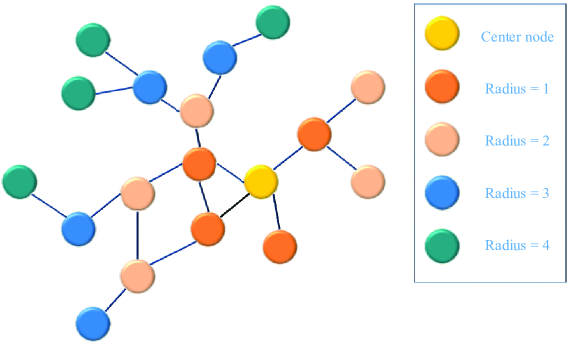
Fig. 1: The example network

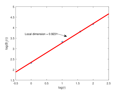
Fig. 2: The relationship in example network

2.4 Fuzzy sets

In the traditional case of things divided into two categories, when there is a class $C$ which is a subset of the universal set $X$, any case of an input variable ${\rm{x}}\in X$ whether belongs to the given subset $C$ or not. There is a characteristic function ${I_{C}}(x)\to\{0,1\}$ which is defined as follows,

$${I_{C}}(x)=\left\{{\begin{array}[]{*{20}{c}}{0,}&{x\in C}\\ {1,}&{x\notin C}\end{array}}\right.$$ (8)

where there is a premise ${\rm{x}}\in X$.

Facing real world situations, there is no clear boundary between two categories or the boundary may be overlapping. So it’s uncertain that the input variable $x$ belongs to the subset $C$ totally. To deal with this problem, this characteristic function must be improved to describe the intermediate value between 0 and 1. L. A. Zadeh[33] proposed the fuzzy sets to modify the characteristic function ${I_{C}}(x)$ to the membership function ${\mu_{C}}(x)$ which can describe the interval continuous function between 0 and 1.

3 Fuzzy local dimension of complex networks

3.1 Basic method

Based on the fuzzy sets and local dimension, a new centrality measure called fuzzy local dimension is proposed. Local dimension focus on the nodes equally whose shortest distance from the center node are less than the box-size. But in general, the node’s contribution is different from each other because of the different distance from the center node. It can be easily obtained that the smaller the distance, the greater the contribution to the center node. To improve this model, fuzzy sets are used to distribute between nodes contributing to the local dimension, and each node within the box-size has a weight through the fuzzy membership function. So the fuzzy local dimension (FLD) is proposed in this paper.

Definition 3.1.

(Fuzzy local dimension). Like the local dimension ${D_{i}}$, the fuzzy local dimension ${D_{fuzzy\_i}}$ is also focus on the local properties of each node, which has the same expression as the local dimension ${D_{i}}$ and is defined as follows,

$${D_{fuzzy\_i}}=\frac{d}{{d\log{r_{t}}}}\log{N_{i}}({r_{t}},\varepsilon)$$ (9)

because of the discrete nature [70, 71] in complex network, the derivative of Eq. (9) is still valid in this case and is expressed as follows,

$${D_{fuzzy\_i}}=\frac{{{r_{t}}}}{{{N_{i}}({r_{t}},\varepsilon)}}\frac{d}{{d{r_{t}}}}{N_{i}}({r_{t}},\varepsilon)$$ (10)

$${D_{fuzzy\_i}}\approx{r_{t}}\frac{{{n_{i}}({r_{t}})}}{{{N_{i}}({r_{t}},\varepsilon)}}$$ (11)

where ${r_{t}}$ is the radius from center node $i$ and it can expand from small to big in a set $\{{\rm{1}},{\rm{2}}\cdots d_{i}^{\max}\}$, ${{n_{i}}({r_{t}})}$ is the fuzzy number of nodes whose shortest distance equal to the box-size $\varepsilon$, ${N_{i}}({r_{t}},\varepsilon)$ is the fuzzy number of nodes whose shortest distance is less than the box-size $\varepsilon$ which is obtained by a fuzzy set, and it can be defined as follows,

$${N_{i}}({r_{t}},\varepsilon){\rm{=}}\frac{{\sum\limits_{j=1}^{N}{{A_{ij}}(\varepsilon)}}}{{{N_{i\_r}}}}$$ (12)

where $\varepsilon$ is the size of box, ${{N_{i\_r}}}$ is the real number of nodes when the shortest distance between node i and j is less than the box size $\varepsilon$, and ${A_{ij}}(\varepsilon)$ is a membership function when the distance from node $j$ to node $i$ is less than the box size $\varepsilon$ which is defined as follows,

$${A_{ij}}(\varepsilon)=\exp(-\frac{{{d_{ij}}^{2}}}{{{\varepsilon^{2}}}})$$ (13)

where ${d_{ij}}$ is the shortest distance between center node $i$ and node $j$. ${A_{ij}}(\varepsilon)$ follows a normal distribution, it can give the neighbour node which is relative to the center node $i$ a weight between 0 and 1 instead of a definite value of 0 or 1. It’s a function of distance and it can distinguish the different nodes whose distance is different from the center node. When the nodes have different distance with center node, these nodes would have different contributions to the center node. When the neighbour node is close to the center node, it would have a bigger weight which is close to 1, and a node’s weight would be a smaller value which is close to 0 when the neighbour node away from the center node. The large the membership function ${A_{ij}}(\varepsilon)$ for node $i$, the greater the contribution to the fuzzy number of nodes ${N_{i}}({r_{t}},\varepsilon)$, and node i would be more influential.

With the membership function ${A_{ij}}(\varepsilon)$, the node’s contribution is not equal to the center node any more. Each node has a individual weight which is relative to the shortest distance from the center node. The closer the node is to the center node, the greater the impact on the center node, the greater the fuzzy number of nodes ${N_{i}}({r_{t}},\varepsilon)$, the more influential the center node. This proposed method is more realistic and effective. When a node is very unimportant, this node’s fuzzy local dimension may be negative, and this property gives a critical basis for identifying the influential nodes.

3.2 Example explanation

In order to explain this proposed method more specific, a small real world complex network named as Kite network [72] is used to explain how this method works. This small network is a interpersonal relation network with ten nodes which is shown in Fig. 3. The Kite network describes the relationships between 10 different people, and it consists of two parts. People in left part (node 1, 2, 3, 4, 5, 6, and 7) are close to each other, and people in right part (node 8, 9, and 10) are not close.

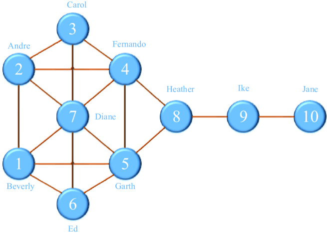
Fig. 3: The Kite network

Step 1: All the nodes in this network will be selected as the center node to calculate its fuzzy local dimension in turn. In this example, node 7 is chosen as the center node first.

Step 2 : The fuzzy number of nodes ${N_{i}}({r_{t}})$ with corresponding radius ${{\rm{r}}_{t}}$ can be obtained by Eq.(12), where the radius ${{\rm{r}}_{t}}$ would expand from 1 to the maximum value of shortest distance $d_{7}^{\max}$ from the center node 7. The fuzzy number of nodes ${N_{7}}({r_{t}})$ when the radius ${{\rm{r}}_{t}}$ equals to 1, 2, 3, and 4 can be respectively obtained as follows,

$$\begin{array}[]{l}{N_{7}}(1)=\frac{{\exp(-\frac{{d_{17}^{2}}}{{{2^{2}}}})+\exp(-\frac{{d_{27}^{2}}}{{{2^{2}}}})+\exp(-\frac{{d_{37}^{2}}}{{{2^{2}}}})+\exp(-\frac{{d_{47}^{2}}}{{{2^{2}}}})+\exp(-\frac{{d_{57}^{2}}}{{{2^{2}}}})+\exp(-\frac{{d_{67}^{2}}}{{{2^{2}}}})+\exp(-\frac{{d_{77}^{2}}}{{{2^{2}}}})}}{7}\\ {\kern 1.0pt}{\kern 1.0pt}{\kern 1.0pt}{\kern 1.0pt}{\kern 1.0pt}{\kern 1.0pt}{\kern 1.0pt}{\kern 1.0pt}{\kern 1.0pt}{\kern 1.0pt}{\kern 1.0pt}{\kern 1.0pt}{\kern 1.0pt}{\kern 1.0pt}{\kern 1.0pt}{\kern 1.0pt}{\kern 1.0pt}{\kern 1.0pt}{\kern 1.0pt}{\kern 1.0pt}{\kern 1.0pt}{\kern 1.0pt}{\kern 1.0pt}{\kern 1.0pt}{\kern 1.0pt}{\kern 1.0pt}{\kern 1.0pt}{\kern 1.0pt}{\kern 1.0pt}{\kern 1.0pt}=\frac{{\exp(-1)+\exp(-1)+\exp(-1)+\exp(-1)+\exp(-1)+\exp(-1)+\exp(0)}}{7}\\ {\kern 1.0pt}{\kern 1.0pt}{\kern 1.0pt}{\kern 1.0pt}{\kern 1.0pt}{\kern 1.0pt}{\kern 1.0pt}{\kern 1.0pt}{\kern 1.0pt}{\kern 1.0pt}{\kern 1.0pt}{\kern 1.0pt}{\kern 1.0pt}{\kern 1.0pt}{\kern 1.0pt}{\kern 1.0pt}{\kern 1.0pt}{\kern 1.0pt}{\kern 1.0pt}{\kern 1.0pt}{\kern 1.0pt}{\kern 1.0pt}{\kern 1.0pt}{\kern 1.0pt}{\kern 1.0pt}{\kern 1.0pt}{\kern 1.0pt}{\kern 1.0pt}{\kern 1.0pt}{\kern 1.0pt}=\frac{{6\times\exp(-1)+\exp(0)}}{7}\\ {\kern 1.0pt}{\kern 1.0pt}{\kern 1.0pt}{\kern 1.0pt}{\kern 1.0pt}{\kern 1.0pt}{\kern 1.0pt}{\kern 1.0pt}{\kern 1.0pt}{\kern 1.0pt}{\kern 1.0pt}{\kern 1.0pt}{\kern 1.0pt}{\kern 1.0pt}{\kern 1.0pt}{\kern 1.0pt}{\kern 1.0pt}{\kern 1.0pt}{\kern 1.0pt}{\kern 1.0pt}{\kern 1.0pt}{\kern 1.0pt}{\kern 1.0pt}{\kern 1.0pt}{\kern 1.0pt}{\kern 1.0pt}{\kern 1.0pt}{\kern 1.0pt}{\kern 1.0pt}{\kern 1.0pt}=0.4582\end{array}$$

$$\begin{array}[]{l}{N_{7}}(2)=\frac{{\exp(-\frac{{d_{17}^{2}}}{{{2^{2}}}})+\exp(-\frac{{d_{27}^{2}}}{{{2^{2}}}})+\exp(-\frac{{d_{37}^{2}}}{{{2^{2}}}})+\exp(-\frac{{d_{47}^{2}}}{{{2^{2}}}})+\exp(-\frac{{d_{57}^{2}}}{{{2^{2}}}})+\exp(-\frac{{d_{67}^{2}}}{{{2^{2}}}})+\exp(-\frac{{d_{77}^{2}}}{{{2^{2}}}})+\exp(-\frac{{d_{78}^{2}}}{{{2^{2}}}})}}{8}\\ {\kern 1.0pt}{\kern 1.0pt}{\kern 1.0pt}{\kern 1.0pt}{\kern 1.0pt}{\kern 1.0pt}{\kern 1.0pt}{\kern 1.0pt}{\kern 1.0pt}{\kern 1.0pt}{\kern 1.0pt}{\kern 1.0pt}{\kern 1.0pt}{\kern 1.0pt}{\kern 1.0pt}{\kern 1.0pt}{\kern 1.0pt}{\kern 1.0pt}{\kern 1.0pt}{\kern 1.0pt}{\kern 1.0pt}{\kern 1.0pt}{\kern 1.0pt}{\kern 1.0pt}{\kern 1.0pt}{\kern 1.0pt}{\kern 1.0pt}{\kern 1.0pt}{\kern 1.0pt}{\kern 1.0pt}=\frac{{\exp(-\frac{1}{4})+\exp(-\frac{1}{4})+\exp(-\frac{1}{4})+\exp(-\frac{1}{4})+\exp(-\frac{1}{4})+\exp(-\frac{1}{4})+\exp(0)+\exp(-1)}}{8}\\ {\kern 1.0pt}{\kern 1.0pt}{\kern 1.0pt}{\kern 1.0pt}{\kern 1.0pt}{\kern 1.0pt}{\kern 1.0pt}{\kern 1.0pt}{\kern 1.0pt}{\kern 1.0pt}{\kern 1.0pt}{\kern 1.0pt}{\kern 1.0pt}{\kern 1.0pt}{\kern 1.0pt}{\kern 1.0pt}{\kern 1.0pt}{\kern 1.0pt}{\kern 1.0pt}{\kern 1.0pt}{\kern 1.0pt}{\kern 1.0pt}{\kern 1.0pt}{\kern 1.0pt}{\kern 1.0pt}{\kern 1.0pt}{\kern 1.0pt}{\kern 1.0pt}{\kern 1.0pt}{\kern 1.0pt}=\frac{{6\times\exp(-\frac{1}{4})+\exp(0)+\exp(-1)}}{8}\\ {\kern 1.0pt}{\kern 1.0pt}{\kern 1.0pt}{\kern 1.0pt}{\kern 1.0pt}{\kern 1.0pt}{\kern 1.0pt}{\kern 1.0pt}{\kern 1.0pt}{\kern 1.0pt}{\kern 1.0pt}{\kern 1.0pt}{\kern 1.0pt}{\kern 1.0pt}{\kern 1.0pt}{\kern 1.0pt}{\kern 1.0pt}{\kern 1.0pt}{\kern 1.0pt}{\kern 1.0pt}{\kern 1.0pt}{\kern 1.0pt}{\kern 1.0pt}{\kern 1.0pt}{\kern 1.0pt}{\kern 1.0pt}{\kern 1.0pt}{\kern 1.0pt}{\kern 1.0pt}{\kern 1.0pt}=0.7551\end{array}$$

$$\begin{array}[]{l}{N_{7}}(3)=\frac{{6\times\exp(-\frac{1}{{{3^{2}}}})+1\times\exp(-\frac{{{2^{2}}}}{{{3^{2}}}})+1\times\exp(-\frac{{{3^{2}}}}{{{3^{2}}}})+1\times\exp(0)}}{9}\\ {\kern 1.0pt}{\kern 1.0pt}{\kern 1.0pt}{\kern 1.0pt}{\kern 1.0pt}{\kern 1.0pt}{\kern 1.0pt}{\kern 1.0pt}{\kern 1.0pt}{\kern 1.0pt}{\kern 1.0pt}{\kern 1.0pt}{\kern 1.0pt}{\kern 1.0pt}{\kern 1.0pt}{\kern 1.0pt}{\kern 1.0pt}{\kern 1.0pt}{\kern 1.0pt}{\kern 1.0pt}{\kern 1.0pt}{\kern 1.0pt}{\kern 1.0pt}{\kern 1.0pt}{\kern 1.0pt}{\kern 1.0pt}{\kern 1.0pt}{\kern 1.0pt}{\kern 1.0pt}{\kern 1.0pt}{\kern 1.0pt}=0.8198\end{array}$$

$$\begin{array}[]{l}{N_{7}}(4)=\frac{{6\times\exp(-\frac{1}{{{4^{2}}}})+1\times\exp(-\frac{{{2^{2}}}}{{{4^{2}}}})+1\times\exp(-\frac{{{3^{2}}}}{{{4^{2}}}})+1\times\exp(-\frac{{{4^{2}}}}{{{4^{2}}}})+1\times\exp(0)}}{{10}}\\ {\kern 1.0pt}{\kern 1.0pt}{\kern 1.0pt}{\kern 1.0pt}{\kern 1.0pt}{\kern 1.0pt}{\kern 1.0pt}{\kern 1.0pt}{\kern 1.0pt}{\kern 1.0pt}{\kern 1.0pt}{\kern 1.0pt}{\kern 1.0pt}{\kern 1.0pt}{\kern 1.0pt}{\kern 1.0pt}{\kern 1.0pt}{\kern 1.0pt}{\kern 1.0pt}{\kern 1.0pt}{\kern 1.0pt}{\kern 1.0pt}{\kern 1.0pt}{\kern 1.0pt}{\kern 1.0pt}{\kern 1.0pt}{\kern 1.0pt}{\kern 1.0pt}{\kern 1.0pt}{\kern 1.0pt}{\kern 1.0pt}=0.8353\end{array}$$

Step 3 : The relationship between fuzzy number of nodes ${N_{7}}({r_{t}})$ and the corresponding radius ${r_{t}}$ can be shown in Fig. 4. The slope of the double logarithmic scale fitting curves is the fuzzy local dimension ${D_{fuzzy\_7}}$ of node 7.

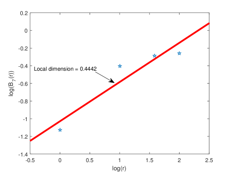
Fig. 4: The double logarithmic scale fitting curves of node 7 in Kite network

Step 4 : Repeat step 1 to step 3 for all remaining nodes, and the results are shown in Table 1.

Node ID	1	2	3	4	5
Fuzzy local dimension	0.3609	0.3609	0.3015	0.4554	0.4554
Node ID	6	7	8	9	10
Fuzzy local dimension	0.3015	0.4442	0.0760	0.0375	-0.1163

Table 1: The fuzzy local dimension of each node in Kite network

Finally, the nodes would be sorted by the value of fuzzy local dimension, and the ranking results with this proposed method and other centrality measures are shown in Table 2. Observing from Table 2 and Table 1, node 4(Fernando) and node 5(Garth) play the most important roles at the same time because they are equivalent to the the door of the parts of the network, and these two nodes’ fuzzy local dimension are also maximum. These two nodes connect two parts of the network. The left part of the network is more complex, so the nodes in this part are more important. Meanwhile, in the left part of Kite network, node 7(Diane) is the center of this part, so it is the most influential node in the left half of the network. The rest nodes in the left part of network including node 1(Beverly), node 2(Andre), node 3(Carol), node 6(Ed) play the same role and they are the edges of this part, the presence of these nodes makes the left part of the network more connected, so they have the same importance. Then, the right part is less important in this network, so these three nodes rank in the last three in the ranking list. But node 8(Heather) is nearest to node 4 and node 5 which are the connection nodes, node 9(Ike) is closer than node 10(Jane), so their importance ranking is 8, 9, 10. This order is the same as the ranking lists obtained by FLD, so the final ranking results from this proposed method (FLD) is more reasonable than others. A detail information in Table 1 is that the fuzzy local dimension of node 10 is negative, and the above conclusion shows node 10 is the least important node of Kite network. So this information shows that the fuzzy local dimension would be negative when one node is far less important than other nodes in the network.

Rank	BC	CC	DC	EC	LD	FLD
1	8	4	7	7	7	4
2	4	5	5	5	4	5
3	9	7	4	4	5	7
4	5	8	2	1	1	2
5	7	2	1	2	2	1
6	2	1	8	6	3	6
7	1	6	6	3	6	3
8	10	3	3	8	9	8
9	6	9	9	9	10	9
10	3	10	10	10	8	10

Table 2: Kite network ranking list with different centrality measures

4 Experimental study

In order to test the effectiveness and accuracy of this proposed method, four real-world complex networks have been applied for this proposed method and some existing methods such as DC, CC, BC, EC, LD. These real-world complex networks include USAir network which can be download from $(http://vlado.fmf.uni-lj.si/pub/networks/data/)$, email network which is from $(http://www.cs.bris.ac.uk/steve/peacockpaper)$, karate network which is from $(http://vlado.fmf.uni-lj.si/pub/networks/data/)$, and Groad network which is from Ref.[73]. These networks’ topological properties are shown in Table 3 respectively.

Network	nodes	edges	$\left\langle k\right\rangle$	${k_{\max}}$	$\left\langle d\right\rangle$	${d_{\max}}$	C
email	1133	10902	9.6222	71	3.6028	8	0.2202
USAir	332	2126	12.8072	139	2.9299	6	0.6252
karate	34	78	4.5882	17	2.3374	5	0.6175
Groad	1168	2486	2.1284	12	19.4024	62	0.0012

Table 3: Topological properties in these four real-world complex networks. Nodes and edges represent the number of nodes and edges in these complex networks respectively; $\left\langle k\right\rangle$ and ${k_{\max}}$ show the average and maximum value of degree; $\left\langle d\right\rangle$ and ${d_{\max}}$ express the average and maximum value of shortest distance; $C$ is the clustering coefficient of these networks.

4.1 Data

BC, DC, CC, EC, LD and this proposed method (FLD) are used for four real-world complex networks to show the performance of this proposed method. The top-10 ranking lists of four real-world complex networks is shown in Table 4 to Table 7. Observing from Table 4 for email network, the proposed method has the same nine node IDs with CC; there are seven same node IDs for the proposed method (FLD) and BC, DC. In Table 5 for USAir network, there are ten same node IDs for the proposed method and CC; FLD has the same nine node IDs with DC; there are six same node IDs for this proposed method and BC. In table 6 for karate network, the proposed method (FLD) has the same eight node IDs with BC; FLD has the same seven and six node IDs with DC and CC. In Table 7 for Groad network, there are nine same node IDs for FLD and CC; there are some differences between this proposed method and BC, DC, and this proposed method has four and two same node IDs with BC and DC respectively. In Table 6 and Table 7, there is a difference between FLD and EC. That’s because these two methods have their own emphasis on the ranking results. EC pays more attention to the whole structure of complex networks, but FLD focuses on the each individuality rather than the whole structure of complex networks. Even if their respective priorities are different, the first few nodes of the ranking result are the same, and the difference of the ranking results obtained by FLD and other centrality measures is relative small. These show that FLD can get a relatively correct influential ranking lists.

This proposed method is better than LD because there are more same nodes with other centrality measures like BC, DC, CC. In email network, FLD has two and four more same node IDs than LD with BC, CC respectively; this proposed method has one more node ID than LD with DC.In USAir network, this proposed method has four and two more same node IDs than LD with CC, BC respectively; this proposed method has equal same node ID with LD comparing with DC. In karate network, FLD has one more node ID than LD with BC, CC, DC. In Groad network, FLD has four more same node IDs than LD with CC, this proposed method has equal same node ID with LD comparing with BC, and there are one less node ID than LD with DC. From the above results, a conclusion can be easily obtained that this proposed method (FLD) is more similar than LD comparing the existed centrality measures.

Rank	BC	CC	DC	EC	LD	FLD
1	23	333	105	105	105	333
2	105	23	333	16	333	23
3	333	105	42	196	23	42
4	76	42	23	204	42	105
5	42	41	16	42	16	76
6	578	76	41	49	434	468
7	135	233	196	56	41	41
8	41	52	233	116	14	233
9	52	135	76	333	468	52
10	355	378	21	3	299	378

Table 4: Email network

Rank	BC	CC	DC	EC	LD	FLD
1	118	118	118	118	118	118
2	8	261	261	261	261	261
3	261	67	255	255	152	67
4	47	255	182	182	230	255
5	201	201	152	152	255	201
6	67	182	230	230	182	182
7	313	47	166	112	112	166
8	13	248	67	67	147	47
9	182	166	112	166	166	248
10	152	112	201	147	293	112

Table 5: USAir network

Rank	BC	CC	DC	EC	LD	FLD
1	1	1	34	34	34	1
2	3	3	1	1	1	34
3	34	34	33	3	33	33
4	33	32	3	33	24	3
5	32	33	2	2	3	2
6	6	14	32	9	2	32
7	2	9	4	14	30	24
8	28	20	24	4	6	28
9	24	2	14	32	7	31
10	9	4	9	31	28	30

Table 6: karate network

Rank	BC	CC	DC	EC	LD	FLD
1	219	698	693	219	219	698
2	543	219	403	217	369	450
3	758	450	300	267	217	565
4	693	565	758	198	565	219
5	886	331	410	207	693	763
6	698	763	373	331	267	267
7	735	267	217	565	295	663
8	403	729	556	236	207	331
9	565	663	331	295	758	295
10	763	347	219	231	331	729

Table 7: Groad network

4.2 Measuring effectiveness by SI model

The standard of susceptible-infected (SI) model is used to test the different centrality measures result and capture the nodes’ influential rank list. In SI model, these nodes are separate into two parts: (1)Susceptible, the number of susceptible nodes at time $t$ is represented by $S(t)$. If one node is susceptible to this disease, this node would be affected by the neighbor nodes to become infected in the next moment. (2)Infected, the number of infected nodes at time $t$ is represented by $I(t)$. If a node is infected, this node has the ability to affect the neighbor nodes. The initial infected nodes $I(0)$ are the test nodes which have been already gotten by previous centrality measures or random given nodes. It can be easily obtained that $S(t)+I(t)=N$, where $N$ the total number of nodes in complex networks. At each time $t$, every infected nodes have the spreading rate $\lambda$ which is defined as $\lambda={(\frac{1}{2})^{\beta}}$ to infect their neighbor susceptible nodes, where $\beta$ has different values in different complex networks. After infection, the node in $S$ state would change to $I$ state. In general, the more influential a node, the stronger its ability to spread, the more the number of nodes infected in a certain time, the more influential this node. The number of infected nodes also can be denoted as $F(t)$, which can be an indicator to measure the importance of the initial given infected nodes at time $t$. It can be easily obtained that $F(t)$ would increase with the development of time $t$, and $F(t)$ would be constant when all nodes have been infected, here it’s denoted as $F({t_{e}})$, where ${t_{e}}$ is the final time when there isn’t node to be infected. Obviously, the higher $F(t)$, the more influential the initial nodes, and $F({t_{e}})$ represents the maximum influence of initial nodes.

According to the property of SI model, a node which has stronger spreading ability is more important in the network. In order to compare the spreading ability of the top-10 nodes between this proposed method and local dimension which are shown in Table 4 to Table 7, SI model is used to simulate the spreading progress of the top-10 nodes and the results of average of 100 independent tests are shown in Fig. 5. After the same time $t$, if the number of infected node $F(t)$ obtained by FLD is greater than LD, it can be shown that the spreading ability of the top-10 nodes obtained by FLD is stronger than obtained by LD, and the opposite case is also true. In Fig. 5, the larger the number of infected node $F(t)$, the larger the vertical value is, the higher the curve is. In order to ensure the accuracy of the experiment and to prevent contingency, the simulation process with different top-10 infected nodes would be performed 100 times. So the curve represents the mean value of 100 experiments, and the error represents the possible interval at each time $t$.

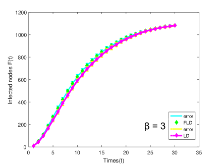
(a) *

Email network

(b)

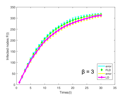
(c) *

USAir network

(d)

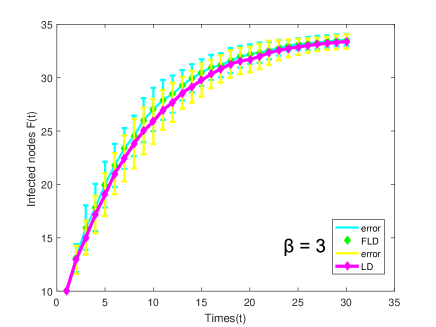
(e) *

Karate network

(f)

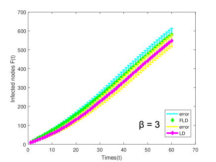
(g) *

Groad network

(h)

Fig. 5: The number of infected nodes with different initial infected nodes (Top-10 nodes in FLD and LD) for four real-world complex networks when $\beta{\rm{=}}3$.

For Email network shown in Fig. 5(a), the initial nodes in this proposed method have stronger spreading ability than LD, because the number of infected nodes $F(t)$ by FLD is larger than LD in the middle infecting progress. For USAir network shown in Fig .5(b), the number of infected nodes $F(t)$ by this proposed method is larger than LD in whole progress, so this proposed method performs better than LD. For Karate network and Groad network shown in Fig .5(c) and Fig .5(d), although the error of average of 100 independent tests is larger than Email network and USAir network, the number of infected nodes $F(t)$ by FLD is larger than LD obviously. So this proposed method outperforms LD. Through these results, an obvious conclusion can be obtained that the initial nodes obtained by this proposed method (FLD) have stronger spreading ability than LD, so FLD is more useful to identify the influential nodes in complex networks.

4.3 Measuring effectiveness by Kendall’s tau coefficient

To measure the correlation between the influential nodes obtained by centrality measures including fuzzy local dimension and the result measured by SI model, Kendall’s tau coefficient[74] which is applied in many fields[75] is used in this paper. The higher the Kendall’s tau coefficient, the more similar the two sequences, the more accurate this proposed method.

Two random variables W and V are assumed, and their $i$th combination is represented as $({W_{i}},{V_{i}})$. If both ${W_{i}}>{W_{j}}$ and ${V_{i}}>{V_{j}}$ or if both ${W_{i}}<{W_{j}}$ and ${V_{i}}<{V_{j}}$ occur at the same time, the $i$th combination $({W_{i}},{V_{i}})$ and $j$th combination $({W_{j}},{V_{j}})$ are considered concordant. If both ${W_{i}}>{W_{j}}$ and ${V_{i}}<{V_{j}}$ or if both ${W_{i}}<{W_{j}}$ and ${V_{i}}>{V_{j}}$ occur at the same time, it means that these two combinations are discordant. And if ${W_{i}}={W_{j}}$ or ${V_{i}}={V_{j}}$, these two combinations are neither concordant nor discordant.

Definition 4.1.

(Kendall’s tau coefficient)Then the Kendall’s tau coefficient $\tau$ is defined[76, 77] as follows,

$$\tau=\frac{{{n_{c}}-{n_{d}}}}{{0.5n(n-1)}}$$ (14)

where $n$ is total combinations in these sequences, ${{n_{c}}}$ and ${{n_{d}}}$ are the the number of concordant combinations and discordant combinations respectively. The higher the Kendall’s tau coefficient $\tau$, the more accurate the centrality measure which is used, and the smaller the $\tau$ is the opposite case. The case $\tau=1$ represents the ranking list by the centrality measures is same as the result obtained by SI model and the case $\tau=0$ is the opposite case.

Kendall’s tau coefficient $\tau$ can clearly show the similarity extent between two centrality measures, and it can use numerical results to intuitively show the correlation. When setting the spreading probability $\lambda$ increasing from 0.01 to 0.1, the Kendall’s tau coefficient $\tau$ would increase with the increasing of spreading probability and it is shown in Fig. 6. It’s clear shown when the correlation between the centrality measures and SI model is higher, the Kendall’s tau coefficient $\tau$ is larger. From Email network in Fig. 6(a), the Kendall’s tau coefficient $\tau$ does not change greatly with the increasing of spreading probability, but the Kendall’s tau coefficient $\tau$ by FLD is large than LD, so this proposed method outperforms LD. In USAir network and Karate network in Fig. 6(b) and (c), the Kendall’s tau coefficient $\tau$ by FLD is much larger than LD, so this proposed method performs better than LD. For Groad network in Fig. 6(d), the Kendall’s tau coefficient $\tau$ by FLD is larger than LD and the result shows that FLD outperforms LD. The comparison between Kendall’s tau coefficient $\tau$ obtained by FLD and LD shows that this FLD outperforms LD and this proposed method is more useful to identify the influential nodes than LD.

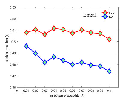
(a)

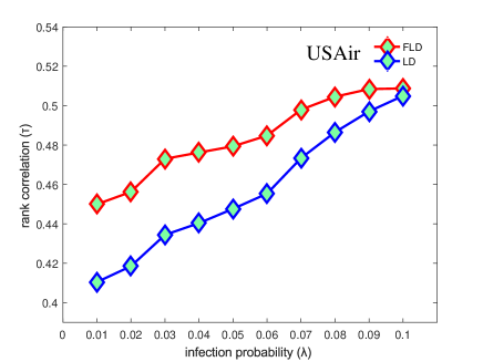
(b)

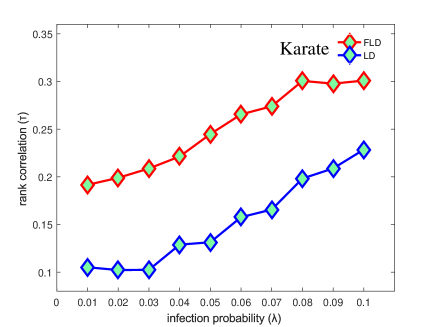
(c)

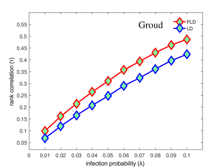
(d)

Fig. 6: The Kendall’s tau coefficient $\tau$ is obtained by FLD, LD and the ranking list from SI model on different networks. The result is the average of 100 independent experiments and the spreading probability $\lambda$ is increasing from 0.01 to 0.1

5 Conclusion

In this paper, a novel fuzzy local dimension is proposed to rank the influential nodes in complex networks. In this method, the nodes with different values of shortest distance from the center node have a different weight to the local dimension of center node by membership function, which is more realistic. The larger the fuzzy local dimension of this center node, the higher ranking the node in the list, the more influential this node. The positive and negative change of the fuzzy local dimension gives a clear demarcation of the ranking list of influential nodes. Compared with other centrality measures, this proposed method focus on each individuality rather than the whole structure of complex networks. Compared with LD, this proposed method takes the different distances from the center node into consideration, and each node within the box-size has a weight through the fuzzy membership function. The node which is closer to the center node would have a greater impact on the center node. Applied to four real-world complex networks, the results from the proposed method (FLD) are in good agreement with the previous centrality measures, and it performs better than LD. Susceptible-Infected (SI) model is used to simulate the spreading progress by different centrality measures, and Kendall’s tau coefficient is used to measure the correlation between the influential nodes obtained by centrality measures including fuzzy local dimension and the result measured by SI model. The results of these four real-world networks applied to these two models show the effectiveness and accuracy of this method.

Reference

References

- [1] P. Deville, C. M. Song, N. Eagle, V. D. Blondel, A. L. Barabasi, and D. S. Wang, “Scaling identity connects human mobility and social interactions,” Proceedings of the National Academy of Sciences of the United States of America, vol. 113, no. 26, pp. 7047–7052, 2016.
- [2] D. S. Wang and C. M. Song, “Impact of human mobility on social networks,” Journal of Communications and Networks, vol. 17, no. 2, pp. 100–109, 2015.
- [3] Z. Q. Zhao, Z. G. Yu, V. Anh, J. Y. Wu, and G. S. Han, “Protein folding kinetic order prediction from amino acid sequence based on horizontal visibility network,” Current Bioinformatics, vol. 11, no. 2, pp. 173–185, 2016.
- [4] K. Hahn, P. R. Massopust, and S. Prigarin, “A new method to measure complexity in binary or weighted networks and applications to functional connectivity in the human brain,” Bmc Bioinformatics, vol. 17, p. 18, 2016.
- [5] J. R. Clough and T. S. Evans, “What is the dimension of citation space?,” Physica a-Statistical Mechanics and Its Applications, vol. 448, pp. 235–247, 2016.
- [6] M. E. J. Newman, “The structure and function of complex networks,” Siam Review, vol. 45, no. 2, pp. 167–256, 2003.
- [7] J. X. Gao, B. Barzel, and A. L. Barabasi, “Universal resilience patterns in complex networks,” Nature, vol. 530, no. 7590, pp. 307–312, 2016.
- [8] C. Hong, J. Zhang, X.-B. Cao, and W.-B. Du, “Structural properties of the Chinese air transportation multilayer network,” CHAOS SOLITONS & FRACTALS, vol. 86, pp. 28–34, 2016.
- [9] X. Li, M. Jusup, Z. Wang, H. Li, L. Shi, B. Podobnik, H. E. Stanley, S. Havlin, and S. Boccaletti, “Punishment diminishes the benefits of network reciprocity in social dilemma experiments,” Proceedings of the National Academy of Sciences, pp. Published online, doi: 10.1073/pnas.1707505115, 2017.
- [10] Z. Wang, M. Jusup, R. W. Wang, L. Shi, Y. Iwasa, Y. Moreno, and J. Kurths, “Onymity promotes cooperation in social dilemma experiments,” Science Advances, vol. 3, no. 3, p. e1601444, 2017.
- [11] Y. Yu, G. Xiao, J. Zhou, Y. Wang, Z. Wang, J. Kurths, and H. J. Schellnhuber, “System crash as dynamics of complex networks,” Proceedings of the National Academy of Sciences, vol. 113, no. 42, pp. 11726–11731, 2016.
- [12] X. Zhang, L. Feng, Y. Berman, N. Hu, and H. E. Stanley, “Exacerbated vulnerability of coupled socio-economic risk in complex networks,” Epl, vol. 116, no. 1, p. 6, 2016.
- [13] X. Lu, H. Mo, and Y. Deng, “An evidential opinion dynamics model based on heterogeneous social influential power,” Chaos Solitons & Fractals, vol. 73, pp. 98–107, 2015.
- [14] E. Rosenberg, “Minimal partition coverings and generalized dimensions of a complex network,” Physics Letters A, 2017.
- [15] S. Pei and H. A. Makse, “Spreading dynamics in complex networks,” Journal of Statistical Mechanics-Theory and Experiment, 2013.
- [16] Z. Wang, C. T. Bauch, S. Bhattacharyya, A. d’Onofrio, P. Manfredi, M. Perc, N. Perra, M. Salathé, and D. Zhao, “Statistical physics of vaccination,” Physics Reports, vol. 664, pp. 1–113, 2016.
- [17] J. Jankowski, P. Brodka, P. Kazienko, B. K. Szymanski, R. Michalski, and T. Kajdanowicz, “Balancing speed and coverage by sequential seeding in complex networks,” Scientific Reports, vol. 7, 2017.
- [18] X. Lu, H. Wang, and Y. Deng, “Evaluating the robustness of temporal networks considering spatiality of connections,” Chaos Solitons & Fractals, vol. 78, pp. 176–184, 2015.
- [19] R. Yang, B.-H. Wang, J. Ren, W.-J. Bai, Z.-W. Shi, W.-X. Wang, and T. Zhou, “Epidemic spreading on heterogeneous networks with identical infectivity,” Physics Letters A, vol. 364, no. 3-4, pp. 189–193, 2007.
- [20] F. Morone, K. Roth, B. Min, H. E. Stanley, and H. A. Makse, “Model of brain activation predicts the neural collective influence map of the brain,” Proceedings of the National Academy of Sciences of the United States of America, vol. 114, no. 15, pp. 3849–3854, 2017.
- [21] S. Wang, Y. Du, and Y. Deng, “A new measure of identifying influential nodes: Efficiency centrality,” Communications in Nonlinear Science and Numerical Simulation, vol. 47, pp. 151–163, 2017.
- [22] L. Lu, D. Chen, X.-L. Ren, Q.-M. Zhang, Y.-C. Zhang, and T. Zhou, “Vital nodes identification in complex networks,” Physics Reports-Review Section of Physics Letters, vol. 650, pp. 1–63, 2016.
- [23] A. Shimbel, “Structural parameters of communication networks,” The bulletin of mathematical biophysics, vol. 15, no. 4, pp. 501–507, 1953.
- [24] L. C. Freeman, “Centrality in social networks conceptual clarification,” Social Networks, vol. 1, no. 3, pp. 215–239, 1979.
- [25] M. E. J. Newman, “A measure of betweenness centrality based on random walks,” Social Networks, vol. 27, no. 1, pp. 39–54, 2005.
- [26] P. Bonacich and P. Lloyd, “Eigenvector-like measures of centrality for asymmetric relations,” Social Networks, vol. 23, no. 3, pp. 191–201, 2001.
- [27] J. Pu, X. Chen, D. Wei, Q. Liu, and Y. Deng, “Identifying influential nodes based on local dimension,” Epl, vol. 107, no. 1, 2014.
- [28] B. Tian and Y. Deng, “A new evidential methodology of identifying influential nodes in complex networks,” Chaos Solitons & Fractals, vol. 103, pp. 101–110, 2017.
- [29] D. Chen, L. Lu, M.-S. Shang, Y.-C. Zhang, and T. Zhou, “Identifying influential nodes in complex networks,” Physica a-Statistical Mechanics and Its Applications, vol. 391, no. 4, pp. 1777–1787, 2012.
- [30] Q. Li, T. Zhou, L. Lu, and D. Chen, “Identifying influential spreaders by weighted leaderrank,” Physica a-Statistical Mechanics and Its Applications, vol. 404, pp. 47–55, 2014.
- [31] L. Lue, Y.-C. Zhang, C. H. Yeung, and T. Zhou, “Leaders in social networks, the delicious case,” Plos One, vol. 6, no. 6, 2011.
- [32] Y. Liu, M. Tang, T. Zhou, and Y. Do, “Identify influential spreaders in complex networks, the role of neighborhood,” Physica a-Statistical Mechanics and Its Applications, vol. 452, pp. 289–298, 2016.
- [33] L. Zadeh, “Fuzzy sets,” Information and Control, vol. 8, no. 3, pp. 338 – 353, 1965.
- [34] W. Pedrycz and X. Wang, “Designing fuzzy sets with the use of the parametric principle of justifiable granularity,” Ieee Transactions on Fuzzy Systems, vol. 24, no. 2, pp. 489–496, 2016.
- [35] W. Pedrycz, “From fuzzy data analysis and fuzzy regression to granular fuzzy data analysis,” Fuzzy Sets and Systems, vol. 274, pp. 12–17, 2015.
- [36] O. Castillo, E. Lizarraga, J. Soria, P. Melin, and F. Valdez, “New approach using ant colony optimization with ant set partition for fuzzy control design applied to the ball and beam system,” Information Sciences, vol. 294, pp. 203–215, 2015.
- [37] O. Castillo, H. Neyoy, J. Soria, P. Melin, and F. Valdez, “A new approach for dynamic fuzzy logic parameter tuning in ant colony optimization and its application in fuzzy control of a mobile robot,” Applied Soft Computing, vol. 28, pp. 150–159, 2015.
- [38] R. Zhang, B. Ashuri, and Y. Deng, “A novel method for forecasting time series based on fuzzy logic and visibility graph,” Advances in Data Analysis and Classification, pp. DOI: 10.1007/s11634–017–0300–3, 2017.
- [39] L. Maciel, R. Ballini, and F. Gomide, “Evolving possibilistic fuzzy modeling for realized volatility forecasting with jumps,” Ieee Transactions on Fuzzy Systems, vol. 25, no. 2, pp. 302–314, 2017.
- [40] W. Jiang, B. Wei, X. Liu, X. Li, and H. Zheng, “Intuitionistic Fuzzy Power Aggregation Operator Based on Entropy and Its Application in Decision Making,” International Journal of Intelligent Systems, pp. Published online, DOI: 10.1002/int.21939, 2017.
- [41] X. Deng and W. Jiang, “An evidential axiomatic design approach for decision making using the evaluation of belief structure satisfaction to uncertain target values,” International Journal of Intelligent Systems, pp. Article in press, doi:10.1002/int.21929, 2017.
- [42] T. Liu, Y. Deng, and F. Chan, “Evidential supplier selection based on DEMATEL and game theory,” International Journal of Fuzzy Systems, pp. DOI: 10.1007/s40815–017–0400–4, 2017.
- [43] L. Fei, H. Wang, L. Chen, and Y. Deng, “A new vector valued similarity measure for intuitionistic fuzzy sets based on OWA operators,” Iranian Journal of Fuzzy Systems, p. accepted, 2017.
- [44] W. Pedrycz, A. Jastrzebska, and W. Homenda, “Design of fuzzy cognitive maps for modeling time series,” Ieee Transactions on Fuzzy Systems, vol. 24, no. 1, pp. 120–130, 2016.
- [45] W. Pedrycz, “From fuzzy models to granular fuzzy models,” International Journal of Computational Intelligence Systems, vol. 9, pp. 35–42, 2016.
- [46] O. Castillo and P. Melin, “Optimization of type-2 fuzzy systems based on bio-inspired methods: A concise review,” Information Sciences, vol. 205, pp. 1–19, 2012.
- [47] O. Castillo, P. Melin, and W. Pedrycz, “Design of interval type-2 fuzzy models through optimal granularity allocation,” Applied Soft Computing, vol. 11, no. 8, pp. 5590–5601, 2011.
- [48] W. Jiang and S. Wang, “An uncertainty measure for interval-valued evidences,” International Journal of Computers Communications & Control, vol. 12, no. 5, pp. 631–644, 2017.
- [49] X. Deng, F. Xiao, and Y. Deng, “An improved distance-based total uncertainty measure in belief function theory,” Applied Intelligence, vol. 46, no. 4, pp. 898–915, 2017.
- [50] X. Zheng and Y. Deng, “Dependence assessment in human reliability analysis based on evidence credibility decay model and iowa operator,” Annals of Nuclear Energy, vol. 112, pp. 673–684, 2018.
- [51] H. Zheng, Y. Deng, and Y. Hu, “Fuzzy evidential influence diagram and its evaluation algorithm,” Knowledge-Based Systems, vol. 131, pp. 28–45, 2017.
- [52] W. Pedrycz and A. Bargiela, “Fuzzy fractal dimensions and fuzzy modeling,” Information Sciences, vol. 153, pp. 199–216, 2003.
- [53] O. Castillo and P. Melin, “Hybrid intelligent systems for time series prediction using neural networks, fuzzy logic, and fractal theory,” Ieee Transactions on Neural Networks, vol. 13, no. 6, pp. 1395–1408, 2002.
- [54] P. Melin and O. Castillo, “An intelligent hybrid approach for industrial quality control combining neural networks, fuzzy logic and fractal theory,” Information Sciences, vol. 177, no. 7, pp. 1543–1557, 2007.
- [55] X. Zhou, X. Deng, Y. Deng, and S. Mahadevan, “Dependence assessment in human reliability analysis based on d numbers and ahp,” Nuclear Engineering and Design, vol. 313, pp. 243–252, 2017.
- [56] Y. Deng, “Deng entropy,” Chaos, Solitons & Fractals, vol. 91, pp. 549–553, 2016.
- [57] H. Mo and Y. Deng, “A new aggregating operator in linguistic decision making based on d numbers,” International Journal of Uncertainty, Fuzziness and Knowledge-Based Systems, vol. 24, no. 6, pp. 831–846, 2016.
- [58] H. Zhang, Y. Hu, X. Lan, S. Mahadevan, and Y. Deng, “Fuzzy fractal dimension of complex networks,” Applied Soft Computing, vol. 25, pp. 514–518, 2014.
- [59] M. Ivanovici and N. Richard, “Fractal dimension of color fractal images,” Ieee Transactions on Image Processing, vol. 20, no. 1, pp. 227–235, 2011.
- [60] M. Bohdalova and M. Gregus, “Fractal analysis of forward exchange rates,” Acta Polytechnica Hungarica, vol. 7, no. 4, pp. 57–69, 2010.
- [61] H. Wang, Z. S. Xu, and W. Pedrycz, “An overview on the roles of fuzzy set techniques in big data processing: Trends, challenges and opportunities,” Knowledge-Based Systems, vol. 118, pp. 15–30, 2017.
- [62] C. M. Song, L. K. Gallos, S. Havlin, and H. A. Makse, “How to calculate the fractal dimension of a complex network: the box covering algorithm,” Journal of Statistical Mechanics-Theory and Experiment, p. 16, 2007.
- [63] H. Zhang, D. Wei, Y. Hu, X. Lan, and Y. Deng, “Modeling the self-similarity in complex networks based on coulomb s law,” Communications in Nonlinear Science and Numerical Simulation, vol. 35, pp. 97–104, 2016.
- [64] L. Lu, T. Zhou, Q. M. Zhang, and H. E. Stanley, “The h-index of a network node and its relation to degree and coreness,” Nature Communications, vol. 7, p. 7, 2016.
- [65] Q. Zhang, M. Li, and Y. Deng, “Measure the structure similarity of nodes in complex networks based on relative entropy,” Physica A: Statistical Mechanics and its Applications, vol. 491, pp. 749–763, 2018.
- [66] T. Zhou, J.-G. Liu, W.-J. Bai, G. Chen, and B.-H. Wang, “Behaviors of susceptible-infected epidemics on scale-free networks with identical infectivity,” Physical Review E, vol. 74, no. 5, 2006.
- [67] D. Wei, X. Chen, and Y. Deng, “Multifractality of weighted complex networks,” Chinese Journal of Physics, vol. 54, no. 3, pp. 416–423, 2016.
- [68] S. Xu, W. Jiang, X. Deng, and Y. Shou, “A modified physarum-inspired model for the user equilibrium traffic assignment problem,” Applied Mathematical Modelling, pp. Article in press, doi: 10.1016/j.apm.2017.07.032, 2017.
- [69] X. Zhang, A. Adamatzky, X.-S. Yang, H. Yang, S. Mahadevan, and Y. Deng, “A physarum-inspired approach to supply chain network design,” Science China Information Sciences, vol. 59, no. 5, p. 052203, 2016.
- [70] E. Ben-Naim, H. Frauenfelder, and Z. Toroczkai, Complex Networks. Springer Berlin Heidelberg, 2004.
- [71] F. N. Silva and L. D. F. Costa, “Local dimension of complex networks,” Computer Science, 2013.
- [72] D. Krackhardt, “Assessing the political landscape: Structure, cognition, and power in organizations,” Administrative Science Quarterly, vol. 35, no. 2, pp. 342–369, 1990.
- [73] M. Kaiser and C. C. Hilgetag, “Spatial growth of real-world networks,” Physical Review E, vol. 69, no. 3, p. 5, 2004.
- [74] P. H. Leslie, “The treatment of ties in ranking problems,” Biometrika, vol. 33, no. 3, pp. 239–251, 1945.
- [75] L. L , D. Chen, X. L. Ren, Q. M. Zhang, Y. C. Zhang, and T. Zhou, “Vital nodes identification in complex networks,” Physics Reports, vol. 650, 2016.
- [76] W. Hoeffding, “A non-parametric test of independence,” Annals of Mathematical Statistics, vol. 19, no. 4, pp. 546–557, 1948.
- [77] M. Hauskrecht, R. Pelikan, M. Valko, and J. Lyonsweiler, Feature Selection and Dimensionality Reduction in Genomics and Proteomics. Springer US, 2007.