Quantum-oscillation-modulated angular dependence of the positive longitudinal magnetoconductivity and planar Hall effect in Weyl semimetals

Abstract

We study the positive longitudinal magnetoconductivity (LMC) and planar Hall effect in Weyl semimetals, following a recent-developed theory by integrating the Landau quantization with Boltzmann equation. It is found that, in the weak magnetic field regime, the LMC and planar Hall conductivity (PHC) obey $\cos^{6}\theta$ and $\cos^{5}\theta\sin\theta$ dependence on the angle $\theta$ between the magnetic and electric fields. For higher magnetic fields, the LMC and PHC cross over to $\cos^{2}\theta$ and $\cos\theta\sin\theta$ dependence, respectively. Interestingly, the PHC could exhibit quantum oscillations with varying $\theta$, due to the periodic-in-$1/B$ oscillations of the chiral chemical potential. When the magnetic and electric fields are noncollinear, the LMC and PHC will deviate from the classical $B$-quadratic dependence, even in the weak magnetic field regime.

I introduction

Since the prediction of Weyl quasiparticles in pyrochlore iridates Wan et al. (2011); Balents (2011), the study of properties of Weyl semimetals (WSMs) in the field of condensed-matter physics, ranging from the unique electronic structures to fascinating topological transports, has attracted much attention on both theoretical and experimental sidesXu et al. (2011); Burkov and Balents (2011); Yang et al. (2011); Halász and Balents (2012); Kim et al. (2013); Hosur and Qi (2013). WSMs are gapless in the bulk, yet possess topologically protected boundary states on the surfaces nonorthogonal to the momentum difference between paired Weyl nodes, which exhibit different topological properties from three-dimensional topological insulators Bernevig and Zhang (2006). Weyl nodes, always coming in pairs in the momentum space, are double degenerate band touching points of the relativistic linear-dispersion excitations Wan et al. (2011); Zyuzin and Burkov (2012); Goswami and Tewari (2013). A pair of Weyl nodes, with chirality quantum number protected by the quantized Berry (or Chern) flux, play the parts of the source and sink of Berry curvature in the momentum space Volovik (2003); Nielsen and Ninomiya (1983). The projections of a pair of bulk Weyl nodes on the surface Brillouin zone are connected by an open Fermi arc of the surface states Wan et al. (2011); Hosur (2012); Okugawa and Murakami (2014); Haldane (2014); Potter et al. (2014); Imura and Takane (2011); Lu et al. (2015).

A Dirac point can split into a pair of Weyl nodes, in the presence of perturbations breaking either the time-reversal or spatial-inversion symmetry. The separation of the Weyl nodes can induce peculiar topological properties, which endow WSMs with multiple interesting physics, such as the positive longitudinal magnetoconductivity (LMC)  Yang et al. (2015); Shekhar et al. (2015); Xiong et al. (2015); Li et al. (2015); Wang et al. (2016); Lv et al. (2017); Huang et al. (2015); Li et al. (2016); Zhang et al. (2016); Zhao et al. (2015); Pan et al. (2017); Du et al. (2016)and giant planar Hall effect Burkov (2017); Nandy et al. (2017). These fascinating magnetotransport phenomena of WSMs are related to the chiral anomaly Nielsen and Ninomiya (1983), which refers to the violation of the separate number conservation laws of Weyl fermions of different chiralities. Nonorthogonal electric and magnetic fields can pump Weyl fermions between Weyl nodes of opposite chiralities, and create a population imbalance between them. The relaxation of the chirality population imbalance contributes an extra electric current to the system, and therefore results in a positive LMC (or negative magnetoresistance) and giant planar Hall conductivity (PHC). The anomalous LMC and PHC, as exotic macroscopic quantum phenomena, have been enjoying a surge of experimental Shekhar et al. (2015); Xiong et al. (2015); Li et al. (2015); Wang et al. (2016); Lv et al. (2017); Huang et al. (2015); Li et al. (2016); Zhang et al. (2016); Zhao et al. (2015); Pan et al. (2017); Du et al. (2016) and theoretical Kim et al. (2013); Aji (2012); Xiao et al. (2017); Son and Spivak (2013); Burkov (2014, 2015) research interest.

While the positive LMC, as a manifested effect of the chiral anomaly in WSMs, has been observed experimentally, its measured dependence on the angle $\theta$ between the electric and magnetic fields turns to be not quite in line with the theoretical predictionsXiong et al. (2015). Primitively, the theory based on the classical Boltzmann theory predicted a $\cos^{2}\theta$ dependence, due to the $B$-quadratic dependence of the chiral anomaly contribution to the conductivity Burkov (2014); Son and Spivak (2013); Burkov (2015); Burkov and Kim (2016); Nandy et al. (2017), where $B$ is magnitude of the magnetic field. The experimentally-observed angular dependence Xiong et al. (2015); Zhang et al. (2016), however, appears to be much stronger than the theoretically-predicted $\cos^{2}\theta$. Burkov connected the angular narrowing phenomenon with the PHC, and argued that the presence of both the LMC with a characteristic angular dependence and giant PHC could be served as a smoking gun signature of the chiral anomaly Burkov (2017). On the other hand, as discussed in Ref.Deng et al. (2019), with increasing the magnetic field, the $B$-quadratic-dependent positive LMC will cross over to be $B$-linearly scaled, which implies that the $\cos^{2}\theta$ dependence will be modified for stronger magnetic fields. Meanwhile, the chiral chemical potential exhibits a periodic-in-$1/B$ quantum oscillation behavior Deng et al. (2019), and therefore the angular dependence of the positive LMC would be very complicated, and their description may be beyond the usual classical theory. It is of importance to understand theoretically how the quantum oscillations of the chiral chemical potential influence the PHC, since it is helpful for us to understand the angular dependence of the magnetoconductivity, and it could also provide new perspectives to experimentally identify WSMs.

In this paper, we follow the theory developed in Ref.Deng et al. (2019) and investigate the effect of quantum oscillations of the chiral anomaly on the PHC and angular dependence of the positive LMC. We find that the LMC $\Delta\sigma_{zz}(B)$ and PHC $\Delta\sigma_{xz}(B)$, in the weak magnetic field regime, are scaled with $B^{2}\cos^{6}\theta$ and $B^{2}\cos^{5}\theta\sin\theta$, respectively, yielding stronger angular dependence than that obtained by Nandy $et$ $al$.Nandy et al. (2017). For higher magnetic fields, i.e., $B\gg E/\upsilon_{\mathrm{F}}$, the angular dependence of the LMC and PHC recover those given by Nandy $et$ $al$, with $\Delta\sigma_{zz}(B)\propto B^{2}\cos^{2}\theta$ and $\Delta\sigma_{xz}(B)\propto B^{2}\cos\theta\sin\theta$. If the Fermi level is slightly way from the Weyl nodes, a step change occurs in the LMC and PHC, as $\theta$ reaches a critical value. For higher Fermi energy, the PHC could oscillate with $\theta$, due to the periodic-in-$1/B$ oscillations in the chiral chemical potential. When the magnetic and electric fields are noncollinear, the LMC and PHC will deviate from the classical $B$-quadratic dependence even in the weak magnetic field regime.

The rest of this paper is organized as follows. In Sec. II, we introduce the model Hamiltonian and solve the spectrum for a WSM in the presence of crossed magnetic and electric fields. The properties of the DOSs and anomalous magnetotransport are analyzed in details in Sec. III and Sec. IV, respectively. The last section contains a summary.

II Hamiltonian and spectrum

Let us consider a WSM subjected to crossed electric and magnetic fields, which can be described by a low-energy effective Hamiltonian $H\mathcal{=}\sum_{\chi}\int d^{3}\mathbf{x}\Psi_{\chi}^{{\dagger}}h_{\chi}(\mathbf{x})\Psi_{\chi}$. The fermion field here is a two-component spinor $\Psi_{\chi}=\exp(i\chi\mathbf{k}_{c}\cdot\mathbf{x})\psi_{\chi}$, which consists of a slowly varying part $\psi_{\chi}=(c_{\chi\uparrow},c_{\chi\downarrow})$ and a rapidly oscillating plane wave with $\chi\mathbf{k}_{c}$ for the momentum locations of the Weyl nodes and $\chi=\pm$ for chiralities, respectively. The Hamiltonian density for each Weyl node is given by

$$h_{\chi}(\mathbf{x})=\hbar\upsilon_{\mathrm{F}}\bm{\sigma}^{\chi}\cdot\mathbf{\Pi}+e\mathcal{A}_{0},$$ (1)

where $\upsilon_{\mathrm{F}}$ denotes the Fermi velocity, $\bm{\sigma}^{\chi}=\chi(\sigma_{x},\sigma_{y},\sigma_{z})$ with $\sigma_{i=x,y,z}$ as the Pauli matrices for electron spin, and $\mathbf{\Pi}=-i\mathbf{\nabla}+e\mathbf{A/}\hbar$ stands for the gauge covariant wave-vector operator modulated by an electromagnetic gauge potential $\mathcal{A}=(\phi,\mathbf{A})$. The electric and magnetic fields are connected to $\mathcal{A}$ by the general relations $\mathbf{E}=-\mathbf{\nabla}\phi$ and $\mathbf{B}=\mathbf{\nabla}\times\mathbf{A}$. Specifically, we fix the electric field to the $z$-direction and confine the magnetic field in the $x$-$z$ plane, i.e., $\mathbf{E}=E\hat{e}_{z}$ and $\mathbf{B}=B(\sin\theta,0,\cos\theta)$, as illustrated in Fig. 1, where $\theta$ is the included angle between the electric and magnetic fields. We choose the Landau gauge $\mathbf{A}=B(x\cos\theta-z\sin\theta)\hat{e}_{y}$ and $\phi=-Ez$. According to the Landau gauge, we rotate the coordinate system, for convenience, about the $y$ axis, i.e., $y^{\prime}=y$ and

$$\left(\begin{array}[c]{c}x^{\prime}\\ z^{\prime}\end{array}\right)=\left(\begin{array}[c]{cc}\cos\theta&-\sin\theta\\ \sin\theta&\cos\theta\end{array}\right)\left(\begin{array}[c]{c}x\\ z\end{array}\right).$$ (2)

Correspondingly, we also perform a unitary transform on the spinor $\psi_{\chi}=e^{-i\frac{\theta}{2}\sigma_{y}}\overline{\psi}_{\chi}$. Then the Hamiltonian, in the rotated coordinate system, can be rewritten as $H\mathcal{=}\sum_{\chi}\int d^{3}\mathbf{x}^{\prime}\overline{\Psi}_{\chi}^{{\dagger}}\overline{h}_{\chi}(\mathbf{x}^{\prime})\overline{\Psi}_{\chi}$, with the Hamiltonian density given by

$$\overline{h}_{\chi}(\mathbf{x}^{\prime})=e^{i(\frac{\theta}{2}\sigma_{y}-\chi\mathbf{k}_{c}\cdot\mathbf{x}^{\prime})}h_{\chi}(\mathbf{x}^{\prime})e^{i(\chi\mathbf{k}_{c}\cdot\mathbf{x}^{\prime}-\frac{\theta}{2}\sigma_{y})}.$$ (3)

In fact, after the coordinate system rotation, the $z^{\prime}$-axis is parallel to the magnetic field. Therefore, the vector potential reduces to $\mathbf{A}^{\prime}=Bx^{\prime}\hat{e}_{y^{\prime}}$ and the scalar potential becomes $\phi(\mathbf{x}^{\prime})=-(E_{\|}z^{\prime}-E_{\bot}x^{\prime})$, where $E_{\|}=E\cos\theta$ and $E_{\bot}=E\sin\theta$.

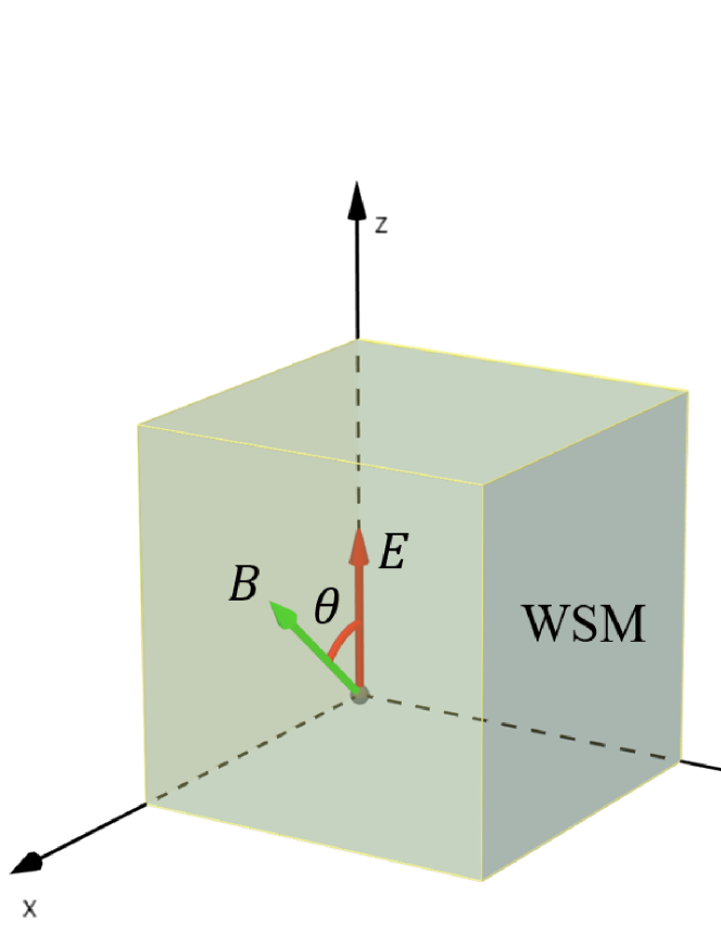
Figure 1: Schematic illustration of a WSM subjected to crossed electric and magnetic fields, in which the electric field is fixed to the $z$-direction and the magnetic field is confined in the $x$-$z$ plane, with $\theta$ as the included angle between the electric and magnetic fields.

To solve the energy spectrum, let us start from the Dirac equation,

$$i\hbar\frac{\partial}{\partial t}\overline{\varphi}^{\chi}(\mathbf{x}^{\prime},t)=\overline{h}_{\chi}(\mathbf{x}^{\prime})\overline{\varphi}^{\chi}(\mathbf{x}^{\prime},t)\ .$$ (4)

The eigenvalue problem of the crossed electric and magnetic fields in graphene has been solved analytically by Lukose $et$ $al$.Lukose et al. (2007), Peres $et$ $al$. Peres and Castro (2007) and Krstajić $et$ $al$.Krstajić and Vasilopoulos (2011). The key step is to find an appropriate Lorentz boost on the time-space coordinate system and a unitary transform on the wavefunction. To implement this procedure, we multiply the both sides of Eq. (4) by $\sigma_{z}$, and then arrive at the covariant time-dependent Dirac equation

$$i\hbar\widetilde{\gamma}^{\mu}(\partial_{\mu}+i\frac{e}{\hbar}\mathcal{A}_{\mu}^{\prime})\overline{\varphi}^{\chi}(x^{\mu})=0$$ (5)

with $x^{0}=\upsilon_{\mathrm{F}}t$ and $x^{1,2,3}=x^{\prime},y^{\prime},z^{\prime}$, where $\widetilde{\gamma}^{0}=\sigma_{z}$, $\widetilde{\gamma}^{1,2}=-i\chi\sigma_{y,x}$ and $\widetilde{\gamma}^{3}=\chi\sigma_{0}$. In order to avoid difficulty in imposing periodic boundary condition along the $z^{\prime}$ directionGreenwood (1958), we denote the parallel (along the magnetic field) component of the electric field by a time-dependent vector potential $\mathcal{A}_{z^{\prime}}=-E_{\|}t$ and then $\mathbf{E}=-\partial_{x^{\prime}}\phi(\mathbf{x}^{\prime})-\partial_{t}\mathcal{A}_{z^{\prime}}$. Therefore, the Dirac equation is translational invariant along the $y^{\prime}$ and $z^{\prime}$ directions. The wavefunction thus can take the form

$$\overline{\varphi}^{\chi}(x^{\mu})=\frac{1}{\sqrt{L_{y^{\prime}}L_{z^{\prime}}}}\sum_{\mathbf{k}}e^{i\mathbf{k}\cdot\mathbf{x}^{\prime}}\overline{\varphi}_{\mathbf{k}}^{\chi}(x^{\prime},t)$$ (6)

with $\mathbf{k}=(0,k_{y},k_{z})$ measured from the corresponding Weyl node and $\mathbf{x}^{\prime}=(x^{\prime},y^{\prime},z^{\prime})$. The parallel electric field enters to $k_{z}$ merely as a parameter by the substitution $k_{z}\rightarrow k_{z}+eE_{\|}t/\hbar$. To eliminate the vertical (perpendicular to the magnetic field) component of the electric field in Eq. (5), we apply a Lorentz boost in the direction parallel to the vector potential

$$\left(\begin{array}[c]{c}\widetilde{x}^{0}\\ \widetilde{x}^{2}\end{array}\right)=\left(\begin{array}[c]{cc}\cosh\vartheta&\sinh\vartheta\\ \sinh\vartheta&\cosh\vartheta\end{array}\right)\left(\begin{array}[c]{c}x^{0}\\ x^{2}\end{array}\right)$$ (7)

with $\vartheta=\tanh^{-1}\frac{E_{\bot}}{\upsilon_{\mathrm{F}}B}$, and then perform a unitary transform on the wavefunction $\overline{\varphi}_{\mathbf{k}}^{\chi}(x^{\prime},t)=e^{-\chi\frac{\vartheta}{2}\sigma_{y}}\widetilde{\varphi}_{\widetilde{\mathbf{k}}}^{\chi}(x^{\prime},\widetilde{t})$. After that we can rewrite Eq. (5) to be

$$(\widetilde{\gamma}^{0}\widetilde{\partial}_{0}+\widetilde{\gamma}^{3}\widetilde{\partial}_{3}+\widetilde{\gamma}^{+}\widetilde{a}_{\xi}+\widetilde{\gamma}^{-}\widetilde{a}_{\xi}^{{\dagger}})\widetilde{\varphi}_{\widetilde{\mathbf{k}}}^{\chi}(x^{\prime},\widetilde{t})=0,$$ (8)

where $\widetilde{\gamma}^{\pm}=(\widetilde{\gamma}^{1}\pm i\widetilde{\gamma}^{2})/(\sqrt{2}\widetilde{l}_{B})$ and $\widetilde{l}_{B}=\eta l_{B}$, with $\eta=(1-\tanh^{2}\vartheta)^{-1/4}$ and $l_{B}=\sqrt{\hbar/eB}$ the magnetic length. The ladder operators are defined as $\widetilde{a}_{\xi}^{{\dagger}}=(\widetilde{\xi}-\widetilde{\partial}_{\xi})/\sqrt{2}$ and $\widetilde{a}_{\xi}=(\widetilde{\xi}+\widetilde{\partial}_{\xi})/\sqrt{2}$, where $\widetilde{\xi}=(x^{\prime}-i\widetilde{l}_{B}^{2}\widetilde{\partial}_{y})/\widetilde{l}_{B}$.

In the boosted frame, we can derive the time component of the four-momentum as $\widetilde{\varepsilon}_{n}^{\chi}=\hbar\upsilon_{\mathrm{F}}\Omega_{n,k_{z}}^{\chi}$, where

$$\Omega_{n,k_{z}}^{\chi}=s_{n}\sqrt{\frac{2|n|}{\widetilde{l}_{B}^{2}}+k_{z}^{2}}-\chi k_{z}\delta_{n,0}$$ (9)

with $s_{n}\equiv\mathrm{sgn}(n)=\{1,0,-1\}$ for $n\{>,=,<\}0$. Subsequently, by the inverse Lorentz boost transformation, we can obtain for the spectrum in the laboratory coordinate system

$$\varepsilon_{n}^{\chi}(k_{y},k_{z})=\eta^{-2}\hbar\upsilon_{\mathrm{F}}\Omega_{n,k_{z}}^{\chi}-\hbar\upsilon_{\mathrm{F}}k_{y}\tanh\vartheta.$$ (10)

The eigenstates corresponding to the spectrum are given by

$$\overline{\varphi}_{\mathbf{k}n}^{\chi}(x^{\prime},t)\propto\frac{e^{-\chi\frac{\vartheta}{2}\sigma_{y}}}{\sqrt{2}}\left(\begin{array}[c]{c}\chi s_{n}\alpha_{n,+}^{\chi}(k_{z})\phi_{|n|-1}(\xi^{\prime})\\ i\alpha_{n,-}^{\chi}(k_{z})\phi_{|n|}(\xi^{\prime})\end{array}\right),$$ (11)

where $\phi_{n}(\xi)$ are the Landau-gauge orbital wavefunctions, $\xi^{\prime}=(x^{\prime}+x_{c}^{\prime})/\widetilde{l}_{B}$ and

$$\alpha_{n,\pm}^{\chi}(k_{z})=\sqrt{1\pm\chi k_{z}/\Omega_{n,k_{z}}^{\chi}}.$$ (12)

When the electric and magnetic fields are collinear, i.e., $\theta=0$, the Landau levels (LLs) are degenerate, with degeneracy equal to $1/2\pi l_{B}^{2}$ per unit cross-section. If the electric and magnetic fields are noncollinear, as shown by Eq. (10), the degeneracy of the LLs will be lifted and simultaneously, the cyclotron centers given by

$$x_{c}^{\prime}=l_{B}^{2}k_{y}+l_{B}^{2}\Omega_{n,k_{z}}^{\chi}\sinh\vartheta$$ (13)

are also renormalized. The spectrums projected to the $k_{y}=0$ plane are plotted in Figs. 2 (a)-(b), from which we can see that the LLs will expand to a sequence of Landau bands (LBs) for $\theta\neq 0$.

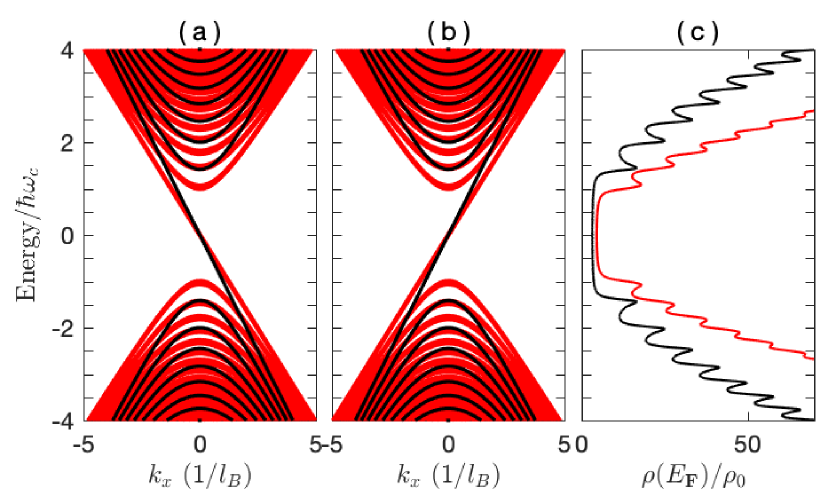
Figure 2: The LLs projected to the $k_{y}=0$ plane for (a) $\chi=+$ and (b) $\chi=-$ Weyl valleys. (c) The DOSs of the Weyl fermions as functions of the Fermi energy, in which the characteristic width of the LLs is chosen as $\Gamma=0.05\hbar\omega_{c}$. The dark (red) curves, for $\theta=0$ ($\pi/5$), represent the electric and magnetic fields are collinear (noncollinear).

The group velocity for the Weyl fermions equals to the slopes of the spectrum $\upsilon_{n,\alpha^{\prime}}^{\chi}=\partial\varepsilon_{n}^{\chi}(k_{y},k_{z})/\hbar\partial k_{\alpha}$. The velocity along the magnetic field

$$\upsilon_{n,z^{\prime}}^{\chi}=\eta^{-2}\upsilon_{\mathrm{F}}(s_{n}\frac{k_{z}}{\sqrt{\frac{2|n|}{\widetilde{l}_{B}^{2}}+k_{z}^{2}}}-\chi\delta_{n,0}),$$ (14)

scaled with $\eta^{-2}=\sqrt{1-\tanh^{2}\vartheta}$, will decrease with increasing $\vartheta$, which is also demonstrated in Fig. 2. As can be seen from Eq. (14) and Fig. 2, the chiral $n=0$ LL is massless, in which the velocity is $k_{z}$-independent, so that the Weyl fermions can not be accelerated by the electric field, while the fermions at the achiral $n\neq 0$ LLs, with nonzero effective mass, will be accelerated by the parallel electric field through $k_{z}+eE_{\|}t/\hbar$. Interestingly, when the magnetic and electric fields are noncollinear, the Weyl fermions, as indicated by the velocity

$$\upsilon_{y}=-\upsilon_{\mathrm{F}}\tanh\vartheta=-\frac{E}{B}\sin\theta,$$ (15)

will drift along the $y$-direction (perpendicular to the electric and magnetic fields). The drifting velocity, irrelevant to the LL and valley indices, is inversely (directly) proportional to the magnetic (vertical electric) field. This result can be understood from the perspective of classical mechanics. In the plane vertical to the magnetic field, there are two forces, i.e., the electric field and Lorentz forces, simultaneously acting on a moving Weyl fermion. As a result, along the direction perpendicular to the electric and magnetic fields, only those fermions with Lorentz force balanced by the electric field force, e.g., $eE_{\bot}=-e\upsilon_{y}B$, can pass through the sample, while others will be totally filtered out. Therefore, by tuning the directions and relative magnitudes of the electric and magnetic fields, one can select velocity [arbitrary directions and magnitudes ($\leqslant\upsilon_{\mathrm{F}}$)] for the Weyl fermions. This simple mechanism can be used to design velocity selector for the Weyl fermions.

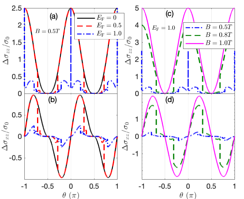
Figure 3: The LMC $\Delta\sigma_{zz}(B)$ (upper panel) and PHC $\Delta\sigma_{xz}(B)$ (lower panel) as functions of the included angle $\theta$ between the magnetic and electric fields for several values of (a, b) the normalized Fermi energy $E_{\mathrm{F}}/\epsilon_{0}$ and (c, d) the magnetic field $B$. Here and hereafter, for convenience, we choose $\sigma_{0}=\frac{2e^{2}}{h}\frac{e[B=1T]\upsilon_{\mathrm{F}}\tau_{\mathrm{inter}}}{h}$ and $\epsilon_{0}=\upsilon_{\mathrm{F}}\sqrt{\hbar e[B=1T]}$ to be units of the conductivity and energy, respectively. The magnetic field in (a, b) is fixed to be $B=0.5T$ and the Fermi energy in (c, d) is set as $E_{\mathrm{F}}=\epsilon_{0}$.

III density of states of WSMs subjected to the crossed magnetic and electric fields

The density of states (DOSs) of a single Weyl valley at the Fermi level can be obtained by the retarded Green’s function

$$\rho(E_{\mathrm{F}})=-\frac{1}{\pi}\operatorname{Im}\sum\limits_{n,k_{y}}\int\frac{dk_{z}}{2\pi}\frac{1}{E_{\mathrm{F}}+i\Gamma-\varepsilon_{n}^{\chi}(k_{y},k_{z})},$$ (16)

where $\Gamma$ characterizes the width of the LLs. The two Weyl valleys have the identical DOSs, whose numerical results are displayed in Fig. 2(c). For $\Gamma\rightarrow 0$, by defining

$$\lambda_{n}(\epsilon)=s_{n}^{2}\sqrt{\epsilon^{2}-2|n|(\eta^{-3}\hbar\omega_{c})^{2}}+\epsilon\delta_{n,0},$$ (17)

the DOSs can be derived to be

$$\rho(E_{\mathrm{F}})=\eta^{2}\rho_{0}\left[2\sum\limits_{n=0}^{n_{c}}\frac{|\lambda_{n}(E_{\mathrm{F},+})-\lambda_{n}(E_{\mathrm{F},-})|}{eE_{\bot}L_{x}}-1\right],$$ (18)

where $E_{\mathrm{F},\pm}=E_{\mathrm{F}}\pm eE_{\bot}L_{x^{\prime}}/2$ and $\rho_{0}=N_{\phi}/h\upsilon_{\mathrm{F}}$, with $N_{\phi}=BS/\phi_{0}$ being the degeneracy of the LLs. Here, $S=L_{x^{\prime}}L_{y^{\prime}}$ is the area of the cross section perpendicular to the magnetic field, and $\phi_{0}=h/e$ is the flux quantum. For a relative weak electric field, we can further simplify the DOSs to be $\rho(E_{\mathrm{F}})=\eta^{2}\rho_{0}\varTheta$, where

$$\varTheta=2\sum\limits_{n=0}^{n_{c}}\frac{1}{\sqrt{1-2|n|(\frac{\eta^{-3}\hbar\omega_{c}}{E_{\mathrm{F}}})^{2}}}-1$$ (19)

with $n_{c}=\mathrm{int}[\frac{1}{2}(\frac{\eta^{3}E_{\mathrm{F}}}{\hbar\omega_{c}})^{2}]$ as the index of the highest (lowest) LB crossed by the Fermi level for $E_{\mathrm{F}}>(<)0$. When the magnetic and electric fields are collinear, Eq. (18) recovers the result given in Ref. Deng et al. (2019), leading to quantum oscillations in the DOSs. Here, the van Hove singularities, determined by

$$E_{\mathrm{F}}=(1-\frac{E^{2}}{\upsilon_{\mathrm{F}}^{2}B^{2}}\sin^{2}\theta)^{3/4}\sqrt{2|n|}\hbar\omega_{c},$$ (20)

are tunable by the included angle and relative magnitudes of the magnetic and electric fields. As a consequence, the quantum oscillations are electrically controllable, as shown by Fig. 2(c).

IV Field and angular dependence of the LMC and PHC

In this section, following the standard Boltzmann approach, we discuss the transport properties of the WSM subjected to the crossed electric and magnetic fields. The steady-state Boltzmann equation for the $n$-th LB of valley $\chi$ is given by

$$\frac{\partial f_{n}^{\chi}}{\partial t}=\frac{\partial f_{n}^{\chi}}{\partial t}|_{d}+\frac{\partial f_{n}^{\chi}}{\partial t}|_{c}=0,$$ (21)

where $f_{n}^{\chi}$ is the nonequilibrium electron distribution function and

$$\frac{\partial f_{n}^{\chi}}{\partial t}|_{d}=\frac{\partial\mathbf{k}}{\partial t}\cdot(\mathbf{\nabla}_{k}\varepsilon_{n}^{\chi})\frac{\partial f_{n}^{\chi}}{\partial\varepsilon_{n}^{\chi}}$$ (22)

is the drifting of the distribution function induced by the external electric field. In the relaxation time approximation, the change of the distribution function due to electron scattering by impurities can be expressed as

$$\frac{\partial f_{n}^{\chi}}{\partial t}|_{c}=\frac{f_{n}^{\chi}-f_{\chi}}{\tau_{\mathrm{intra}}}+\frac{f_{n}^{\chi}-f_{g}}{\tau_{\mathrm{inter}}}$$ (23)

with $\tau_{\mathrm{intra}}$ and $\tau_{\mathrm{inter}}$ being relaxation times due to electron intravalley and intervalley scattering by impurities, respectively. $f_{\chi}$ and $f_{g}=(f_{\chi}+f_{-\chi})/2$ represent the local and global equilibrium electron distribution functions for the system. Therefore, Eq. (21) can be rewritten as

$$e\mathbf{E}\cdot\mathbf{\upsilon}_{n}^{\chi}(\mathbf{k})\frac{\partial f_{n}^{\chi}}{\partial\varepsilon_{n}^{\chi}}=-\frac{f_{n}^{\chi}-f_{\chi}}{\tau_{\mathrm{intra}}}-\frac{f_{n}^{\chi}-f_{g}}{\tau_{\mathrm{inter}}}.$$ (24)

Within the framework of the linear response, the electron distribution function takes the general form

$$f_{n}^{\chi}(\mathbf{k})=f_{0}(\varepsilon_{n}^{\chi})+[-\partial_{\varepsilon_{n}^{\chi}}f_{0}(\varepsilon_{n}^{\chi})]g_{n}^{\chi}(\mathbf{k}),$$ (25)

where $f_{0}(\epsilon)=1/[1+e^{\beta(\epsilon-E_{\mathrm{F}})}]$ stands for the electron equilibrium distribution function, and $g_{n}^{\chi}(\mathbf{k})$ describes the deviation of $f_{n}^{\chi}(\mathbf{k})$ from $f_{0}(\varepsilon_{n}^{\chi})$ due to the applied external fields. Substitution of Eq. (25) into Eq. (24) leads to

$$e\mathbf{E}\cdot\mathbf{\upsilon}_{n}^{\chi}(\mathbf{k})=-\frac{g_{n}^{\chi}(\mathbf{k})-\overline{g}_{\chi}}{\tau_{\mathrm{intra}}}-\frac{g_{n}^{\chi}(\mathbf{k})-\overline{g}}{\tau_{\mathrm{inter}}}$$ (26)

with $\overline{g}_{\chi}=\langle g_{n}^{\chi}(\mathbf{k})\rangle_{\chi}$ and $\overline{g}=(\overline{g}_{\chi}+\overline{g}_{-\chi})/2$. The average $\langle\cdots\rangle_{\chi}$ here is defined as

$$\langle\cdots\rangle_{\chi}=\frac{\sum_{n,k_{y}}\int[-\partial_{\varepsilon_{n}^{\chi}}f_{0}(\varepsilon_{n}^{\chi})](\cdots)dk_{z}}{\sum_{n,k_{y}}\int[-\partial_{\varepsilon_{n}^{\chi}}f_{0}(\varepsilon_{n}^{\chi})]dk_{z}},$$ (27)

in which the summation runs over all electron states at the Fermi level in the $\chi$ valley.

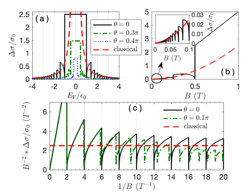
Figure 4: Amplitude of the LMC and PHC $\Delta\sigma(B)$ versus (a) the normalized Fermi level $E_{\mathrm{F}}/\epsilon_{0}$, (b) the magnetic field $B$ (weak magnetic field parameter region) and (c) the reciprocal of the magnetic field $1/B$ (strong magnetic field parameter region). The parameters are the same as Fig. 3.

In the absence of the intervalley scattering, the system can not reach the global equilibrium. As a result, for a given chirality, even at full momentum relaxation of the electron distribution, there exists a finite electric current proportional to the chirality imbalance, which predicts an unphysical diverging electrical conductivity. However, in a real system, the conductivity can never be infinite. This implies that the intervalley scattering must exist to relax the system to global equilibrium between the valleys. The emergence of the LMC requires that the intravalley scattering must be stronger than the intervalley scattering, i.e., $\tau_{\mathrm{intra}}/\tau_{\mathrm{inter}}\ll 1$. In this situation, the system would be relaxed to the local equilibrium first by the intravalley scattering and to the global equilibrium later by the intervalley scattering. This process would produce a finite chemical potential difference between the two Weyl valleys, half of which is usually called as the chiral chemical potential. In the opposite limit, $\tau_{\mathrm{intra}}/\tau_{\mathrm{inter}}\gg 1$, which may occur in Dirac semimetals, where the energy bands are doubly degenerate, no chiral chemical potential exists, since the system would be relaxed to the global equilibrium, directly.

In the following, we would consider $\tau_{\mathrm{intra}}/\tau_{\mathrm{inter}}\ll 1$, such that we can safely approximate $g_{n}^{\chi}(\mathbf{k})=\overline{g}_{\chi}$ in the second term of Eq. (26), and obtain for

$$eE_{\|}\upsilon_{n,z^{\prime}}^{\chi}(\mathbf{k})=-\frac{g_{n}^{\chi}(\mathbf{k})-\overline{g}_{\chi}}{\tau_{\mathrm{intra}}}-\frac{\overline{g}_{\chi}-\overline{g}_{-\chi}}{2\tau_{\mathrm{inter}}},$$ (28)

where $\overline{g}_{\chi}=\chi\Delta\mu$. Here, due to the cyclotron motion, the Weyl fermions, in the plane perpendicular to the magnetic field, are localized by the strong magnetic field. Accordingly, we can solve for

$$g_{n}^{\chi}(\mathbf{k})=-eE_{\|}\upsilon_{n,z^{\prime}}^{\chi}(\mathbf{k})\tau_{\mathrm{intra}}+\chi(1-\frac{\tau_{\mathrm{intra}}}{\tau_{\mathrm{inter}}})\Delta\mu.$$ (29)

By averaging the both sides of Eq. (29), we can determine $\Delta\mu$ self-consistently to be

$$\Delta\mu=-\chi eE_{\|}\langle\upsilon_{n,z^{\prime}}^{\chi}(\mathbf{k})\rangle_{\chi}\tau_{\mathrm{inter}}=\frac{eE_{\|}}{2\pi l_{B}^{2}}\frac{\tau_{\mathrm{inter}}}{\mathcal{F}},$$ (30)

where

$$\mathcal{F}=\frac{2\pi\hbar}{S}\int_{-\infty}^{\infty}[-\partial_{\epsilon}f_{0}(\epsilon)]\rho(\epsilon)d\epsilon.$$ (31)

The electrical current density can be calculated by

$$j_{\alpha}=\frac{e}{2\pi S}{\displaystyle\sum\limits_{\chi,n,k_{y}}}\int\upsilon_{n,\alpha}^{\chi}(\mathbf{k})g_{n}^{\chi}(\mathbf{k})\partial_{\varepsilon_{n}^{\chi}}f_{0}(\varepsilon_{n}^{\chi})dk_{z}$$ (32)

and the conductivity tensor is defined as $\sigma_{\alpha z}=j_{\alpha}/E$. By substituting Eq. (29) into Eq. (32), we derive the conductivity along the electric field to be

$$\sigma_{zz}(B)=[\sigma_{D}+\Delta\sigma(B)]\cos^{2}\theta,$$ (33)

where the amplitude is given by

$$\Delta\sigma(B)=\frac{2e^{2}}{h}\frac{(eB)^{2}}{h^{2}}\frac{\tau_{\mathrm{inter}}-\tau_{\mathrm{intra}}}{\mathcal{F}}$$ (34)

and $\sigma_{D}=\frac{2e^{2}\upsilon_{\mathrm{F}}\tau_{\mathrm{intra}}}{h}\mathcal{F}_{1}$, with

$$\mathcal{F}_{1}=\frac{1}{2\pi\widetilde{l}_{B}^{2}}\int_{-\infty}^{\infty}[-\partial_{\epsilon}f_{0}(\epsilon)]\Lambda(\epsilon)d\epsilon$$ (35)

and

$$\Lambda(\epsilon)=2{\displaystyle\sum\limits_{n=0}^{n_{c}}}\sqrt{1-2n(\frac{\eta^{-3}\hbar\omega_{c}}{\epsilon})^{2}}-1.$$ (36)

The PHC can be obtained as

$$\sigma_{xz}(B)=[\sigma_{D}+\Delta\sigma(B)]\cos\theta\sin\theta.$$ (37)

It is noted that Eqs. (33) and (37) are applicable to the case of strong magnetic field. For weak magnetic fields, the electrons are weakly localized by the magnetic field, such that there could exist electric current in the plane perpendicular to the magnetic field. However, it does not affect our discussions on the LMC and planar Hall effect, since the electric current in the plane perpendicular to the magnetic field mainly contributes to the Drude conductivity $\sigma_{D}$, and, as discussed below, $\sigma_{D}$ is almost independent on the magnetic field.

Before analyzing the numerical results, we can infer some properties of the LMC and PHC. At low temperatures, by the approximation $-\partial_{\epsilon}f_{0}(\epsilon)=\delta(\epsilon-E_{\mathrm{F}})$, we can reduce $\Delta\mu$ to be

$$\Delta\mu=\eta^{-2}eE_{\|}l_{e}\frac{1}{\varTheta}$$ (38)

with $l_{e/a}=\upsilon_{\mathrm{F}}\tau_{\mathrm{inter}/\mathrm{intra}}$. Subsequently, we can arrive at

$$\sigma_{D}=\eta^{-2}\frac{2e^{2}}{h}\frac{eBl_{a}}{h}\Lambda(E_{\mathrm{F}})$$ (39)

and

$$\Delta\sigma(B)=\eta^{-2}\frac{2e^{2}}{h}\frac{eB(l_{e}-l_{a})}{h}\varTheta^{-1}.$$ (40)

In the weak magnetic field regime i.e., $|E_{\mathrm{F}}|\gg\hbar\omega_{c}$, by taking the replacement $\sum\limits_{n=0}^{n_{c}}\rightarrow\int_{0}^{n_{c}}dn$ in Eq. (19), we derive $\varTheta\simeq 2(\eta^{3}E_{\mathrm{F}}/\hbar\omega_{c})^{2}$ and $\Lambda(E_{\mathrm{F}})\simeq\eta^{6}\frac{\pi hn_{e}}{eBk_{\mathrm{F}}}$, with $n_{e}=k_{\mathrm{F}}^{3}/3\pi^{2}$ being the carrier density. Therefore, $\sigma_{D}=\eta^{4}\frac{e^{2}n_{e}}{\hbar k_{\mathrm{F}}}\upsilon_{\mathrm{F}}\tau_{\mathrm{intra}}$ is just the zero-field Drude conductivity and $\Delta\sigma(B)=\eta^{-6}\Delta\sigma_{0}(B)$ with

$$\Delta\sigma_{0}(B)=\frac{e^{2}}{4\pi^{2}\hbar}\frac{(eB)^{2}\upsilon_{\mathrm{F}}^{2}}{E_{\mathrm{F}}^{2}}\upsilon_{\mathrm{F}}\tau_{\mathrm{inter}}$$ (41)

being the LMC for $\theta=0$, where we have neglected the term tied to $\tau_{\mathrm{intra}}$ in $\Delta\sigma_{0}(B)$ for $\tau_{\mathrm{intra}}\ll\tau_{\mathrm{inter}}$. Therefore, the LMC and PHC reduce to the classical form

$$\Delta\sigma_{zz}(B) =(1-\tanh^{2}\vartheta)^{2}\Delta\sigma_{0}(B)\cos^{2}\theta,$$ (42)

$$\Delta\sigma_{xz}(B) =(1-\tanh^{2}\vartheta)^{2}\Delta\sigma_{0}(B)\cos\theta\sin\theta.$$ (43)

As can be seen, the amplitude of the LMC has $B^{2}$ dependence for any value of $\theta$ except for $\theta=\pi/2$, and the $B$-quadratic dependence holds for the PHC when $\theta\neq 0,\pi/2$. Similar formula were shown by Nandy $et$ $al$.Nandy et al. (2017), which predicted a $\cos^{2}\theta$ angular dependence of the LMC and a $\cos\theta\sin\theta$ angular dependence of the PHC. However, the experimentally-observed angular dependence of the LMC appeared to be much stronger than the theoretically-predicted $\cos^{2}\theta$, which is not quite consistent with the expectations drawn from the previous theoryXiong et al. (2015); Zhang et al. (2016). As different from the formula derived by Nandy $et$ $al$., our results, in addition to the $\cos^{2}\theta$ and $\cos\theta\sin\theta$ factors, contain another angle-dependent factor $(1-\tanh^{2}\vartheta)^{2}$. In the weak magnetic limit, e.g., $B\rightarrow E/\upsilon_{\mathrm{F}}$, by the approximation $1-\tanh^{2}\vartheta\simeq\cos^{2}\theta$, our results predict stronger angular dependence for the LMC and PHC, with $\Delta\sigma_{zz}(B)\propto B^{2}\cos^{6}\theta$ and $\Delta\sigma_{xz}(B)\propto B^{2}\cos^{5}\theta\sin\theta$. For higher magnetic fields, i.e., $B\gg E/\upsilon_{\mathrm{F}}$ ($\tanh\vartheta\rightarrow 0$), the angular dependence returns to that given by Nandy $et$ $al$., i.e., the $\cos^{6}\theta$ ($\cos^{5}\theta\sin\theta$) angular dependence of the LMC (PHC) will cross over to the $\cos^{2}\theta$ ($\cos\theta\sin\theta$) dependence.

The above inferences are confirmed by the numerical results shown in Fig. 3, where we plot the calculated $\Delta\sigma_{zz}(B)$ and $\Delta\sigma_{xz}(B)$ as functions of $\theta$ for several values of the normalized Fermi energy $E_{\mathrm{F}}/\epsilon_{0}$ and the magnetic field $B$. As demonstrated in the classical formula, i.e., Eqs. (41)-(43), the amplitude of the LMC and PHC, in addition to the $B$-quadratic dependence, are scaled with $1/E_{\mathrm{F}}^{2}$, which show an unphysical diverging character if $E_{\mathrm{F}}=0$, as presented by the red dash line in Fig. 4(a). In the ultra-quantum limit, however, the LMC and PHC remain finite for $E_{\mathrm{F}}=0$, as can be seen from the dark-solid curves in Figs. 3(a), (c) and Fig. 4(a). In fact, the case of $E_{\mathrm{F}}=0$ is equivalent to the strong magnetic field regime, in which only the $n=0$ LL is crossed by the Fermi level. In this limiting case, Eq. (40) can be simplified to

$$\Delta\sigma(B)\simeq\eta^{-2}\frac{2e^{2}}{h}\frac{eB\upsilon_{\mathrm{F}}\tau_{\mathrm{inter}}}{h},$$ (44)

which predicts an $E_{\mathrm{F}}$-independence and $B$-linear dependence of the LMC and PHC, as also shown by Fig. 4(b). The $B$-linear dependence of the positive LMC has been observed recently, based on Weyl orbits in Cd₃As₂Zhang et al. (2018). For a finite but relative small $E_{\mathrm{F}}$, e.g., $E_{\mathrm{F}}\sim 0.5\epsilon_{0}$, a step change occurs in the LMC and planar Hall conductivity when $\theta$ reaches a critical value, as indicated by the red-dash curves in Figs. 3(a) and (c). To explain the sudden change of $\Delta\sigma_{zz}(B)$ and $\Delta\sigma_{xz}(B)$, we plot $\Delta\sigma(B)$, the amplitude of the LMC and PHC, as functions of the normalized Fermi level $E_{\mathrm{F}}/\epsilon_{0}$ in Fig. 4(a). As it shows, $\Delta\sigma(B)$ oscillates strongly with $E_{\mathrm{F}}$, due to the van Hove singularities in the DOSs. As shown by Eq. (40), the DOSs enter $\Delta\sigma(B)$ as a denominator. As a consequence, when the Fermi level encounters a van Hove singularity where the DOSs increase dramatically, $\Delta\sigma(B)$ will be suppressed heavily. For fixed $E_{\mathrm{F}}$ and $B$, with $\theta$ increasing from $0$, the van Hove singularities, as depicted in Fig. 4(a), would shift towards the zero energy point, and then sweep over the Fermi level, leading to the sudden drops in Figs. 3(a) and (c). When $E_{\mathrm{F}}$ is in the vicinity of the van Hove singularities, the LMC, as $\theta$ shifts away from $0$, decays rapidly with a decaying rate far faster than $\cos^{2}\theta$, as seen from the blue-dash-dot curve in Fig. 3(a). For larger $E_{\mathrm{F}}$, with $\theta$ or $B$ varying, more van Hove singularities pass through the Fermi level, which results in the oscillation behavior of $\Delta\sigma(B)$ in Fig. 4(b), as also can be seen from the blue-dash-dot curves in Fig. 3. As shown by Figs. 3(c) and (d), the classical angular dependence of the LMC and planar Hall conductivity can be recovered by increasing the magnetic field.

With further increasing the magnetic field, the number of the LBs intersected by the Fermi level will decrease, and as a result, the magnetic-field dependence of the LMC and PHC would, gradually, deviate from the $B$-quadratic dependence, as demonstrated in Fig. 4(b). Though the LMC oscillates strongly with $B$, its classical $B$-quadratic dependence for weak magnetic field limit can be reflected by the envelope of $\Delta\sigma(B)$, as shown in the inset of Fig. 4(b). In the strong magnetic field regime $\hbar\omega_{c}>|E_{\mathrm{F}}/\sqrt{2}|$, where the Fermi level only crosses the $n=0$ LL, the $B$-quadratic dependence of $\Delta\sigma(B)$ will finally cross over to the $B$-linear dependence, as shown by Fig. 4(b).

When the magnetic and electric fields are collinear, $\Delta\sigma(B)$ exhibits a periodic-in-$1/B$ oscillation, with the period given byDeng et al. (2019)

$$\Delta(\frac{1}{B})=2e\hbar(\frac{\upsilon_{\mathrm{F}}{}}{E_{\mathrm{F}}})^{2}.$$ (45)

The periodic-in-$1/B$ oscillation is depicted by the dark solid curve of Fig. 4(c). The periodic-in-$1/B$ oscillation is attributable to the van Hove singularities, i.e., Eq. (45) is solved via Eq. (20) by setting $\theta=0$. When the magnetic and electric fields are noncollinear, the classical $B$-quadratic dependence of the LMC and PHC will be modified even in the weak magnetic regime, as shown by the cyan dash-dot curve of Fig. 4(c).

V summary

In summary, based on the theory developed recently, we have studied the properties of the magnetotransport in WSMs. It is found that the LMC and PHC are, respectively, scaled with $B^{2}\cos^{6}\theta$ and $B^{2}\cos^{5}\theta\sin\theta$ for weak magnetic field regime. For higher magnetic fields, the angular dependence of the LMC and PHC cross over to $\cos^{2}\theta$ and $\cos\theta\sin\theta$ dependence. In the strong magnetic field regime, when the Fermi level is slightly way from the Weyl nodes, a step change would occur in the LMC and PHC, as $\theta$ reaches a critical value. With $\theta$ increasing from $0$, the $B$-quadratic dependence of the LMC and PHC will be modified even in the weak magnetic regime.

VI acknowledgements

This work was supported by the National Natural Science Foundation of China under Grants No. 11474106 (R.-Q.W), No. 11674160 (L.S.), No. 11804130 (W.L.), No. 11804101 (W.Y.D.), the Key Program for Guangdong NSF of China under Grant No. 2017B030311003 (R.-Q.W) and GDUPS(2017).

References

- Wan et al. (2011) X. Wan, A. M. Turner, A. Vishwanath, and S. Y. Savrasov, Phys. Rev. B 83, 205101 (2011).
- Balents (2011) L. Balents, Physics 4, 36 (2011).
- Xu et al. (2011) G. Xu, H. Weng, Z. Wang, X. Dai, and Z. Fang, Phys. Rev. Lett. 107, 186806 (2011).
- Burkov and Balents (2011) A. A. Burkov and L. Balents, Phys. Rev. Lett. 107, 127205 (2011).
- Yang et al. (2011) K.-Y. Yang, Y.-M. Lu, and Y. Ran, Phys. Rev. B 84, 075129 (2011).
- Halász and Balents (2012) G. B. Halász and L. Balents, Phys. Rev. B 85, 035103 (2012).
- Kim et al. (2013) H.-J. Kim, K.-S. Kim, J.-F. Wang, M. Sasaki, N. Satoh, A. Ohnishi, M. Kitaura, M. Yang, and L. Li, Phys. Rev. Lett. 111, 246603 (2013).
- Hosur and Qi (2013) P. Hosur and X. Qi, Comptes Rendus Physique 14, 857 (2013).
- Bernevig and Zhang (2006) B. A. Bernevig and S.-C. Zhang, Phys. Rev. Lett. 96, 106802 (2006).
- Zyuzin and Burkov (2012) A. A. Zyuzin and A. A. Burkov, Phys. Rev. B 86, 115133 (2012).
- Goswami and Tewari (2013) P. Goswami and S. Tewari, Phys. Rev. B 88, 245107 (2013).
- Volovik (2003) G. E. Volovik, The universe in a helium droplet, vol. 117 (Oxford University Press on Demand, 2003).
- Nielsen and Ninomiya (1983) H. Nielsen and M. Ninomiya, Phys. Lett. B 130, 389 (1983).
- Hosur (2012) P. Hosur, Phys. Rev. B 86, 195102 (2012).
- Okugawa and Murakami (2014) R. Okugawa and S. Murakami, Phys. Rev. B 89, 235315 (2014).
- Haldane (2014) F. D. M. Haldane, arXiv:1401.0529 (2014).
- Potter et al. (2014) A. C. Potter, I. Kimchi, and A. Vishwanath, Nat. Commun. 5, 5161 (2014).
- Imura and Takane (2011) K.-I. Imura and Y. Takane, Phys. Rev. B 84, 245415 (2011).
- Lu et al. (2015) B. Lu, K. Yada, M. Sato, and Y. Tanaka, Phys. Rev. Lett. 114, 096804 (2015).
- Yang et al. (2015) L. X. Yang, Z. K. Liu, Y. Sun, H. Peng, H. F. Yang, T. Zhang, B. Zhou, Y. Zhang, Y. F. Guo, M. Rahn, et al., Nat. Phys. 11, 728 (2015).
- Shekhar et al. (2015) C. Shekhar, A. K. Nayak, Y. Sun, M. Schmidt, M. Nicklas, I. Leermakers, U. Zeitler, Y. Skourski, J. Wosnitza, Z. Liu, et al., Nat. Phys. 11, 645 (2015).
- Xiong et al. (2015) J. Xiong, S. K. Kushwaha, T. Liang, J. W. Krizan, M. Hirschberger, W. Wang, R. J. Cava, and N. P. Ong, Science 350, 413 (2015).
- Li et al. (2015) C.-Z. Li, L.-X. Wang, H. Liu, J. Wang, Z.-M. Liao, and D.-P. Yu, Nat. Commun. 6, 10137 (2015).
- Wang et al. (2016) Y. Wang, E. Liu, H. Liu, Y. Pan, L. Zhang, J. Zeng, Y. Fu, M. Wang, K. Xu, Z. Huang, et al., Nat. Commun. 7, 13142 (2016).
- Lv et al. (2017) Y.-Y. Lv, X. Li, B.-B. Zhang, W. Y. Deng, S.-H. Yao, Y. B. Chen, J. Zhou, S.-T. Zhang, M.-H. Lu, L. Zhang, et al., Phys. Rev. Lett. 118, 096603 (2017).
- Huang et al. (2015) X. Huang, L. Zhao, Y. Long, P. Wang, D. Chen, Z. Yang, H. Liang, M. Xue, H. Weng, Z. Fang, et al., Phys. Rev. X 5, 031023 (2015).
- Li et al. (2016) H. Li, H. He, H.-Z. Lu, H. Zhang, H. Liu, R. Ma, Z. Fan, S.-Q. Shen, and J. Wang, Nat. Commun. 7, 10301 (2016).
- Zhang et al. (2016) C.-L. Zhang, S.-Y. Xu, I. Belopolski, Z. Yuan, Z. Lin, B. Tong, G. Bian, N. Alidoust, C.-C. Lee, S.-M. Huang, et al., Nat. Commun. 7, 10735 (2016).
- Zhao et al. (2015) Y. Zhao, H. Liu, J. Yan, W. An, J. Liu, X. Zhang, H. Wang, Y. Liu, H. Jiang, Q. Li, et al., Phys. Rev. B 92, 041104(R) (2015).
- Pan et al. (2017) X.-C. Pan, Y. Pan, J. Jiang, H. Zuo, H. Liu, X. Chen, Z. Wei, S. Zhang, Z. Wang, X. Wan, et al., Frontiers of Physics 12, 127203 (2017).
- Du et al. (2016) J. Du, H. Wang, Q. Mao, R. Khan, B. Xu, Y. Zhou, Y. Zhang, J. Yang, B. Chen, C. Feng, et al., Sci. China-Phys. Mech. Astron. 59, 657406 (2016).
- Burkov (2017) A. A. Burkov, Phys. Rev. B 96, 041110 (2017).
- Nandy et al. (2017) S. Nandy, G. Sharma, A. Taraphder, and S. Tewari, Phys. Rev. Lett. 119, 176804 (2017).
- Aji (2012) V. Aji, Phys. Rev. B 85, 241101 (2012).
- Xiao et al. (2017) X. Xiao, K. T. Law, and P. A. Lee, Phys. Rev. B 96, 165101 (2017).
- Son and Spivak (2013) D. T. Son and B. Z. Spivak, Phys. Rev. B 88, 104412 (2013).
- Burkov (2014) A. A. Burkov, Phys. Rev. Lett. 113, 247203 (2014).
- Burkov (2015) A. A. Burkov, Phys. Rev. B 91, 245157 (2015).
- Burkov and Kim (2016) A. A. Burkov and Y. B. Kim, Phys. Rev. Lett. 117, 136602 (2016).
- Deng et al. (2019) M.-X. Deng, G. Y. Qi, R. Ma, R. Shen, R.-Q. Wang, L. Sheng, and D. Y. Xing, Phys. Rev. Lett. 122, 036601 (2019).
- Lukose et al. (2007) V. Lukose, R. Shankar, and G. Baskaran, Phys. Rev. Lett. 98, 116802 (2007).
- Peres and Castro (2007) N. M. R. Peres and E. V. Castro, J. Phys. C 19, 406231 (2007).
- Krstajić and Vasilopoulos (2011) P. M. Krstajić and P. Vasilopoulos, Phys. Rev. B 83, 075427 (2011).
- Greenwood (1958) D. A. Greenwood, Proc. Phys. Soc. 71, 585 (1958).
- Zhang et al. (2018) C. Zhang, Y. Zhang, X. Yuan, S. Lu, J. Zhang, A. Narayan, Y. Liu, H. Zhang, Z. Ni, R. Liu, et al., Nature (2018).