Intuitive joint priors for variance parameters

Abstract

Variance parameters in additive models are typically assigned independent priors that do not account for model structure. We present a new framework for prior selection based on a hierarchical decomposition of the total variance along a tree structure to the individual model components. For each split in the tree, an analyst may be ignorant or have a sound intuition on how to attribute variance to the branches. In the former case a Dirichlet prior is appropriate to use, while in the latter case a penalised complexity (PC) prior provides robust shrinkage. A bottom-up combination of the conditional priors results in a proper joint prior. We suggest default values for the hyperparameters and offer intuitive statements for eliciting the hyperparameters based on expert knowledge. The prior framework is applicable for R packages for Bayesian inference such as INLA and RStan.

Three simulation studies show that, in terms of the application-specific measures of interest, PC priors improve inference over Dirichlet priors when used to penalise different levels of complexity in splits. However, when expressing ignorance in a split, Dirichlet priors perform equally well and are preferred for their simplicity. We find that assigning current state-of-the-art default priors for each variance parameter individually is less transparent and does not perform better than using the proposed joint priors. We demonstrate practical use of the new framework by analysing spatial heterogeneity in neonatal mortality in Kenya in 2010–2014 based on complex survey data.

1 Introduction

Bayesian hierachical models (BHMs) are ubiquitous in science due to their flexibility and interpretablity (Gelman and Hill, 2007; Gelman et al., 2013; Banerjee et al., 2014). In this paper, we consider BHMs where the latent level consists of an additive combination of model components that are classified as fixed effects and random effects. This subclass covers a range of common model classes such as generalised linear mixed models (GLMMs) and generalised additive mixed models (GAMMs) (Fahrmeir and Lang, 2001). In additive models, the total latent variance of the sum of the random effects decomposes into the sum of the variance contributed by each random effect, and each random effect has a variance parameter that controls its a priori contribution. We present a general framework for constructing joint priors for these variance parameters for BHMs, and suggest robust shrinkage priors for the reduced class of latent Gaussian models (LGMs) where the model components are Gaussian conditional on the model parameters (Rue et al., 2009, 2017; Bakka et al., 2018; Krainski et al., 2018).

There is no concensus on priors for variance parameters in BHMs (Lambert et al., 2005; Gelman, 2006; Gelman et al., 2017a). The default prior in the R package INLA (Lindgren and Rue, 2015) is an inverse-gamma distribution $\text{InvGamma}(1,5\cdot 10^{-5})$ (Blangiardo and Cameletti, 2015), and the R package RStan (Carpenter et al., 2017; Stan Development Team, 2018b) has implicit priors that are uniform on the range of legal values for the parameters (Stan Development Team, 2018c). WinBUGS, OpenBUGS and JAGS used $\text{InvGamma}(0.001,0.001)$ distributions in their examples (Spiegelhalter et al., 1996; Plummer, 2017), and the Stata manual employs $\text{InvGamma}(0.01,0.01)$ priors (StataCorp, 2017). Conjugacy provides $\text{InvGamma}(\epsilon,\epsilon)$ distributions with computational advantages, but their use may result in severe problems (Gelman, 2006) and they are generally inappropriate for variances of random effects (Lunn et al., 2009). Gelman (2006) proposed heavier tails through $\text{Half-Cauchy}(25)$ distributions on the standard deviations, and others have investigated bounded uniform densities on the variances or the logarithms of the variances (Lambert et al., 2005) and bounded uniform priors on the standard deviations (Martinez-Beneito, 2013). Recently, Simpson et al. (2017) proposed a principle-based, robust prior termed penalised complexity (PC) prior that offers shrinkage towards zero variance. In the case of LGMs, the PC prior is an exponential distribution on the standard deviation.

However, general-purpose priors may not be suitable for a given application (Gelman et al., 2017b) and independent priors for each random effect cannot exploit the structure of the model (Simpson et al., 2017, Section 7). For example, in disease mapping, prior elicitation is more meaningful for the total variance of the random effects than their separate variances (Wakefield, 2006), and, for animal models in genetic settings, the proportion of variability in a phenotypic trait being accounted for by genes is important (Holand et al., 2013). Further, the intraclass correlation (ICC) (McGraw and Wong, 1996) in a random intercept model is linked to a generalised version of the coefficient of determination (Gelman and Hill, 2007), also known as $R^{2}$, which expresses the proportion of the total variance explained by the model components. However, putting a prior on $R^{2}$ requires a joint prior on the two variance parameters in the random intercept model. Additionally, in the context of regression, Som et al. (2014) discuss block g-priors where regression coefficients are partitioned and shrinkage is applied to the $R^{2}$ of each partition.

Consider a simple multilevel model with responses $y_{i,j,k}|\eta_{i,j,k}\sim\text{Poisson}(\exp(\eta_{i,j,k}))$, where $\eta_{i,j,k}=a_{i}+b_{i,j}+c_{i,j,k}$ for experiment $k$ on individual $j$ in group $i$. We will term the group effect, individual effect and measurement effect for A, B, and C, respectively, and write the latent model as A+B+C for short hand. The total latent variance $t$ of A+B+C decomposes as $t=\sigma_{\mathrm{A}}^{2}+\sigma_{\mathrm{B}}^{2}+\sigma_{\mathrm{C}}^{2}$, where $\sigma_{\mathrm{A}}^{2}$, $\sigma_{\mathrm{B}}^{2}$ and $\sigma_{\mathrm{C}}^{2}$ are the variances of A, B and C, respectively. This standard parametrization facilitates independent priors on the variances and can be used to achieve the desired a priori marginal properties for the random effects. However, it is difficult to encode a priori knowledge on joint properties such as the size of $t$ or preference for A over B or A+B over C in a transparent and intuitive way.

An obvious alternative is to parametrize the variance parameters as $t$ and the proportion of $t$ assigned to each random effect $(\omega_{\mathrm{A}},\omega_{\mathrm{B}},\omega_{\mathrm{C}})$, where $0\leq\omega_{\mathrm{A}},\omega_{\mathrm{B}},\omega_{\mathrm{C}}\leq 1$ and $\omega_{\mathrm{A}}+\omega_{\mathrm{B}}+\omega_{\mathrm{C}}=1$. This is illustrated in Figure 1(a) by splitting A+B+C into the models A, B and C. This parametrization is suitable for expressing ignorance about how the variance should be attributed to the random effects. A simple way to assign the joint prior is to set $(\omega_{\mathrm{A}},\omega_{\mathrm{B}},\omega_{\mathrm{C}})\sim\text{Dir}(a,a,a)$, $a>0$, where Dir denotes the Dirichlet distribution (Balakrishnan and Nevzorov, 2003). This prior has no preference for one of the random effects over the other and is invariant to the ordering of the random effects, and we can select $a>0$ to make the prior suitably vague. Together with the conditional prior $\pi(t|\omega_{\mathrm{A}},\omega_{\mathrm{B}},\omega_{\mathrm{C}})$, this implicitly defines a proper joint prior for $(\sigma_{\mathrm{A}}^{2},\sigma_{\mathrm{B}}^{2},\sigma_{\mathrm{C}}^{2})$ that is invariant to permutations in the order of the random effects, but can incorporate prior knowledge on $t$. This has a similar flavor as the Dirichlet-Laplace prior by Bhattacharya et al. (2015), which is a global-local shrinkage prior (Polson and Scott, 2010) that induces sparsity in regression. However, in this paper we will focus on random effects and not fixed effects.

(a) Unstructured

(b) Structured

(c) Structured shrinkage

Figure 1: Hierarchical model decomposition. Gray boxes indicate preferred branches.

The simple split strategy is not always suitable and Riebler et al. (2016) demonstrated that for the BYM (Besag, York and Mollié) model, which is a sum of a Besag random effect and an unstructured random effect, a PC prior that penalises the added complexity of the structured effect relative to the unstructured effect improves inference. For A+B+C, fewer levels of hierarchy may be preferred so that B is preferred to A and C is preferred over A+B. This knowledge about relative complexity of the random effects can be incorporated by splitting A+B+C hierarchically as shown in Figure 1(b). Here we first split A+B+C into A+B and C through $\omega_{1}=(\sigma_{\mathrm{A}}^{2}+\sigma_{\mathrm{B}}^{2})/t$, and then split A+B into A and B through $\omega_{2}=\sigma_{\mathrm{A}}^{2}/(\sigma_{\mathrm{A}}^{2}+\sigma_{\mathrm{B}}^{2})$, where $0\leq\omega_{1},\omega_{2}\leq 1$. The joint prior for $(\sigma_{\mathrm{A}}^{2},\sigma_{\mathrm{B}}^{2},\sigma_{\mathrm{C}}^{2})$ is then constructed by first selecting $\pi(\omega_{2})$, then $\pi(\omega_{1}|\omega_{2})$, and finally $\pi(t|\omega_{1},\omega_{2})$. Priors inducing shrinkage towards $\omega_{2}=0$ and $\omega_{1}=0$ can be chosen in the lower and upper split, respectively. The shrinkage can be illustrated graphically as shown in Figure 1(c). For LGMs, PC priors offer a robust choice, but the framework is general and other priors can be selected by the analyst. For example, if shrinkage is only required at the top level, a Dirichlet prior for $(\omega_{2},1-\omega_{2})$ could be combined with a shrinkage prior for $\omega_{1}|\omega_{2}$.

The ideas generalize to more random effects through the selection of a hierarchical decomposition of the model in the form of a tree, and the selection of a conditional distribution for the attribution of the total variance to the branches for each split. The joint prior is calculated in a bottom-up approach using these conditional distributions. We suggest default values for the hyperparameters of the Dirichlet distribution based on the marginal prior distributions for the proportions of variance assigned to each branch of the split. This ensures that the default setting for the prior is well-behaved as the number of branches in a split increases. Default values for the PC priors can be selected based on moderate shrinkage of the proportion of variance. Additionally, we discuss how to include expert knowledge through interpretable statements on the total variance and the distribution of variance in the tree. The joint prior can contain a mix of expert knowledge and default values that provide a weakly informative prior (Gelman et al., 2008; Simpson et al., 2017). This means the prior framework with joint priors is appropriate for default priors for software packages such as INLA and RStan.

The properties of the proposed priors are compared to the properties of default priors from software and vague priors from literature. This is a fair comparison since even though the new priors account for model structure, they do not incorporate strong expert knowledge and are suggested to be used in a default way in Bayesian software. The comparison is performed through three simulation studies: a simple random intercept model with Gaussian responses, a latin square experiment with Gaussian responses, and a spatial model with Binomial responses. To ease the presentation of the comparisons and not overload the reader with results, we choose a set of targets for each simulation study and compare the posteriors resulting from the different prior choices with respect to the targets. Additional results are provided in the Supplementary Materials. Furthermore, we provide example code in the Supplementary Materials for producing results for different priors for the latin square model in Section 5.2. The code is described in Section S4.3 in the Supplementary Materials.

We start by introducing the general framework in Section 2, then we introduce LGMs and suitable priors for developing a new class of priors for LGMs in Section 3. The new class of priors for LGMs is introduced in Section 4 and is applied to simulation studies with Gaussian responses in Section 5. In Section 6 we present one simulation study with Binomial response and explain how the approach can be used in practice. The paper ends with a discussion in Section 7.

2 Tree-based hierarchical variance decomposition

In this section we cover basic notation, and formally introduce additive models, hierarchical variance decomposition, and the new framework for joint priors for variances.

2.1 Additive models

Let $\bm{y}=(y_{1},\ldots,y_{n})$ be a vector of $n>0$ observations. We model the expected values $\mathrm{E}(y_{i})=g^{-1}(\eta_{i})$, $i=1,\ldots,n$, through a vector of linear predictors $\bm{\eta}=(\eta_{1},\ldots,\eta_{n})$ and a link function $g:\mathbb{R}\rightarrow\mathbb{R}$. We consider models where the likelihood has parameters $\bm{\theta}_{\mathrm{L}}$ and factors as $\pi(\bm{y}|\bm{\eta},\bm{\theta}_{\mathrm{L}})=\prod_{i=1}^{n}\pi(y_{i}|\eta_{i},\bm{\theta}_{\mathrm{L}})$. This covers models such as GLMMs and GAMMs. We term $\bm{\eta}$ and its description as the latent part of the model.

We assume that the linear predictor is described as

$$\eta_{i}=\beta_{0}+\bm{x}_{i}^{\mathrm{T}}\bm{\beta}+\sum_{j=1}^{N}u_{j,k_{j}[i]},\quad i=1,\ldots,n,$$ (2.1)

where $\beta_{0}$ is the intercept, $\bm{x}_{i}$ is the vector of covariates associated with observation $i$, $\bm{\beta}$ is a vector of coefficients, and $\bm{u}_{j}=(u_{1},\ldots,u_{m_{j}})$ is a random vector and $k_{j}[i]$ is the associated element of $\bm{u}_{j}$ for observation $i$ for $j=1,\ldots,N$. The two first terms will be called fixed effects and the last $N$ terms will be called random effects. To focus on the joint prior for variance parameters, we will assume that each random effect $\bm{u}_{j}$ has a single model parameter, which is a variance $\sigma_{j}^{2}$. In general, the random effects may have other parameters such as correlation parameters and we discuss how to handle this in Section 7.

We denote the vector of model parameters by $\bm{\theta}_{\mathrm{M}}=(\sigma_{1}^{2},\ldots,\sigma_{N}^{2})$. The BHM is completed by specifying the latent model through $\pi(\bm{u}_{j}|\sigma_{j}^{2})$ for $j=1,\ldots,N$, and the prior $\pi(\beta_{0},\bm{\beta},\bm{\theta}_{\mathrm{L}},\bm{\theta}_{\mathrm{M}})$. We follow common practice so that the prior satisfies $\pi(\beta_{0},\bm{\beta},\bm{\theta}_{\mathrm{L}},\bm{\theta}_{\mathrm{M}})=\pi(\beta_{0})\pi(\bm{\beta})\pi(\bm{\theta}_{\mathrm{L}})\pi(\bm{\theta}_{\mathrm{M}})$. The major improvement over common practice is that we will develop a framework for selecting intuitive joint priors for the variance parameters that does not require that $\pi(\bm{\theta}_{\mathrm{M}})=\prod_{j=1}^{N}\pi(\sigma_{j}^{2})$.

2.2 Hierarchical variance decomposition

The additivity in Equation (2.1) causes the total latent variance $\text{Var}[\eta_{i}|\beta_{0},\bm{\beta},\bm{\theta}_{\mathrm{M}}]$ of linear predictor $i$ to decompose as the variance contributed by each random effect $\text{Var}[u_{k_{j}[i]}|\beta_{0},\bm{\beta},\sigma_{j}^{2}]$, $j=1,\ldots,N$, for $i=1,\ldots,n$. If random effect j is homogeneous, the variance parameter of random effect $j$ will be a marginal variance in the sense that $\text{Var}[u_{k_{j}[i]}|\beta_{0},\bm{\beta},\sigma_{j}^{2}]=\sigma_{j}^{2}$ for $i=1,\ldots,n$. If all random effects are homogeneous, the total latent variance of the linear predictors is homogeneous, $t=\text{Var}[\eta_{1}|\beta_{0},\bm{\beta},\bm{\theta}_{\mathrm{M}}]=\cdots=\text{Var}[\eta_{n}|\beta_{0},\bm{\beta},\bm{\theta}_{\mathrm{M}}]=\sigma_{1}^{2}+\ldots+\sigma_{N}^{2}$. If random effect $j$ is heterogenous so that $\text{Var}[u_{k_{j}[i]}|\beta_{0},\bm{\beta},\sigma_{j}^{2}]$ varies for different values of $i$, the variance parameter $\sigma_{j}^{2}$ is selected to be comparable to a marginal variance; see the discussion in Section 3.1. We term the parameter $t=\sigma_{1}^{2}+\ldots+\sigma_{N}^{2}$ the total latent variance.

We describe the attribution of $t$ to the individual random effects through a tree $\mathcal{T}$. The construction of $\mathcal{T}$ starts with a root node $T_{0}=\{1,\ldots,N\}$ that contains all the random effects, and in the first step we introduce $K_{1}>1$ child nodes $T_{1},\ldots,T_{K_{1}}$ that partition $T_{0}$ into $T_{0}=T_{1}\cup\cdots\cup T_{K_{1}}$. We continue this recursively for each child node until all leaf nodes are singletons. This results in a tree $\mathcal{T}$ with $S$ splits where there are $K_{s}$ child nodes for split $s=1,\ldots,S$. We have $S\leq N-1$, where $S=1$ is achieved by directly splitting the root node to singletons as in Figure 1(a) and the maximum value is achieved by only using dual splits such as in Figure 1(b).

For each split $s$, the parent node $P_{s}$ is split into $K_{s}$ child nodes $C_{1},\ldots,C_{K_{s}}$ and we will define a vector of parameters $\bm{\omega}_{s}=(\omega_{s,1},\ldots,\omega_{s,K_{s}})$, $s=1,\ldots,S$. The child nodes describe a partitioning of the random effects in the parent node, and we let $\bm{\omega}_{s}$ describe the proportion of the total variance in the parent node, $\sum_{j\in P_{s}}\sigma_{j}^{2}$, that is assigned to each child node through

$$\bm{\omega}_{s}=\frac{1}{\sum_{j\in P_{s}}\sigma_{j}^{2}}\left(\sum_{j\in C_{1}}\sigma_{j}^{2},\ldots,\sum_{j\in C_{K_{s}}}\sigma_{j}^{2}\right),\quad s=1,\ldots,S.$$

We denote the $K-1$ simplex by $\Delta^{K}=\{(x_{1},\ldots,x_{K})|\sum_{k=1}^{K}x_{k}=1,x_{k}\geq 0\,\,\,\forall k\}$ so that the restrictions are $\bm{\omega}_{s}\in\Delta^{K_{s}}$ for $s=1,\dots,S$. This means that the parameters $\omega_{s,K_{s}}$ are superfluous for $s=1,\ldots,S$, but we keep them for ease of notation and interpretability.

For any split $s=1,\ldots,S$, we term a child node and its decendants as a branch of the split. The description of the model structure through a tree structure defines a re-parametrization of $(\sigma_{1}^{2},\ldots,\sigma_{N}^{2})$ to $(t,\bm{\omega}_{1},\ldots,\bm{\omega}_{S})$, where $S$ is the number of splits in the tree. The examples discussed in the introduction can be rephrased in this terminology, and demostrate that there is no unique selection of the tree.

Example 1 (Tree structure).

Consider three random effects A, B and C with marginal variances $(\sigma_{\mathrm{A}}^{2},\sigma_{\mathrm{B}}^{2},\sigma_{\mathrm{C}}^{2})$. Let the root node be $T_{0}=\{\mathrm{A},\mathrm{B},\mathrm{C}\}$.

Figure 1(a), describes the case that the root node is partitioned into three children $T_{1}=\{\mathrm{A}\}$, $T_{2}=\{\mathrm{B}\}$ and $T_{3}=\{\mathrm{C}\}$. This leads to a reparametrization $(t,\bm{\omega})$, where $t=\sigma_{\mathrm{A}}^{2}+\sigma_{\mathrm{B}}^{2}+\sigma_{\mathrm{C}}^{2}$ and $\bm{\omega}=(\sigma_{\mathrm{A}}^{2},\sigma_{\mathrm{B}}^{2},\sigma_{\mathrm{C}}^{2})/t$.

Figure 1(b) shows the case that $T_{0}$ is first partitioned into $T_{1}=\{\mathrm{A},\mathrm{B}\}$ and $T_{2}=\{\mathrm{C}\}$, and then $T_{1}$ is partitioned into $T_{3}=\{\mathrm{A}\}$ and $T_{4}=\{\mathrm{B}\}$. This results in a reparamerization $(t,\bm{\omega}_{1},\bm{\omega}_{2})$, where $t=\sigma_{\mathrm{A}}^{2}+\sigma_{\mathrm{B}}^{2}+\sigma_{\mathrm{C}}^{2}$, $\bm{\omega}_{1}=(\sigma_{\mathrm{A}}^{2}+\sigma_{\mathrm{B}}^{2},\sigma_{\mathrm{C}}^{2})/t$ and $\bm{\omega}_{2}=(\sigma_{\mathrm{A}}^{2},\sigma_{\mathrm{B}}^{2})/(\sigma_{\mathrm{A}}^{2}+\sigma_{\mathrm{B}}^{2})$.  $\triangle$

2.3 Hierachical decomposition priors

The tree-based hierarchical variance decomposition facilitates the construction of joint priors that include prior belief about the relative sizes of groups of random effects. The tree structure must be selected so that the desired comparisons can be made. Trees such as shown in Figure 1(a) are useful for expressing ignorance about the attribution of variance to the random effects, whereas trees such as shown in Figure 1(b) are useful for imposing shrinkage to one of the branches in each dual split. Generally, a tree may consist of a mixture of splits where the analyst wants to be informative and splits where the analyst wants to express ignorance.

We propose to construct a joint prior for the marginal variance parameters in a bottom-up approach where the prior for a given split only depends on descendant nodes of the parent node.

Assumption 1 (Bottom-up approach).

For a tree structure with $S$ splits, $\pi(\{\bm{\omega}_{s}\}_{s=1}^{S})=\prod_{s=1}^{S}\pi(\bm{\omega}_{s}|\{\bm{\omega}_{j}\}_{j\in D(s)}),$ where $D(s)$ is the set of decscendant splits for split $s=1,\ldots,S$.

This means that the joint prior for the decomposition uses a directed acyclic graph so that parameters that belong to subsplits in different branches of a split are marginally independent. We combine the prior for the decomposition of the variance with a conditional prior on the total variance of the random effects to form what we will call hierarchical decomposition (HD) priors.

Definition 1 (Hierarchical decomposition (HD) priors).

Consider a BHM with an additive latent structure with $N$ random effects with marginal variance parameters $\sigma_{1}^{2},\ldots,\sigma_{N}^{2}$. Assume that the model structure is described by a tree that recursively partitions the set of random effects into singletons. Then a hierarchical decomposition (HD) prior is given by

$$\pi(\sigma_{1}^{2},\ldots,\sigma_{N}^{2})=\pi(t|\{\bm{\omega}_{s}\}_{s=1}^{S})\prod_{s=1}^{S}\pi(\bm{\omega}_{s}|\{\bm{\omega}_{j}\}_{j\in D(s)}),$$

where $t=\sigma_{1}^{2}+\ldots+\sigma_{N}^{2}$, $S$ is the number of splits, and $D(s)$ denotes the set of descendant splits for the parent node in split $s$ and $\bm{\omega}_{s}$ describes the proportions of the total variance of a parent node assigned to its branches for $s=1,\ldots,S$.

3 Latent Gaussian models and priors for the splits

This section introduces LGMs and the priors we will use for the splits to build the intuitive class of joint priors for the variance parameters for LGMs.

3.1 Latent Gaussian models

LGMs constitute a subclass of BHMs with additive latent structure where the model components are Gaussian conditional on the model parameters. We write the additive model in Equation (2.1) in vector form, $\bm{\eta}=\bm{1}\beta_{0}+\mathbf{X}\bm{\beta}+\sum_{j=1}^{N}\mathbf{A}_{j}\bm{u}_{j},$ where $\bm{1}=(1,\ldots,1)$ is a column vector of length $n$, $\mathbf{X}$ is the $n\times p$ design matrix that contains the covariates for each observation as rows, and $\mathbf{A}_{j}$ are sparse $n\times m_{j}$ matrices that select the appropriate elements of the random effects for $j=1,\ldots,N$. The latent Gaussian structure is achieved by $\beta_{0}\sim\mathcal{N}(0,\sigma_{\mathrm{I}}^{2})$, $\bm{\beta}\sim\mathcal{N}_{p}(\bm{0},\sigma_{\mathrm{F}}^{2}\mathbf{I}_{p})$, and $\bm{u}_{j}|\sigma_{j}^{2}\sim\mathcal{N}_{m_{j}}(\bm{0},\sigma_{j}^{2}\Sigma_{j})$ for $j=1,\ldots,N$. It is common to give $\sigma_{\mathrm{I}}^{2}$ and $\sigma_{\mathrm{F}}^{2}$ suitably vague values, and we will assume that $\sigma_{\mathrm{I}}^{2}$ and $\sigma_{\mathrm{F}}^{2}$ are fixed and focus on the variance parameters $\sigma_{1}^{2},\ldots,\sigma_{N}^{2}$.

For non-intrinsic Gaussian random effects, such as independent and identically distributed (i.i.d.) random effects, stationary autoregressive processes and Matérn Gaussian random fields, the covariance matrix $\Sigma$ of the random effect $\bm{u}$ is chosen to be a correlation matrix and the variance parameter $\sigma^{2}$ is the marginal variance. However, this does not work for intrinsic Gaussian Markov random fields (GMRFs) (Rue and Held, 2005) such as the Besag model (Besag et al., 1991), the first-order random walk and the second-order random walk (Rue and Held, 2005, Chapter 3). In this case there is no well-defined concept of a marginal variance since they are defined through singular precision matrices that cannot be inverted to find a covariance matrix. We follow Sørbye and Rue (2014) and choose the variance parameter $\sigma^{2}$ to be a representative value for the marginal variance.

3.2 Introducing shrinkage towards branches

Penalising complexity

The fundamental basis for introducing robust shrinkage in our proposed class of priors are the PC priors introduced in Simpson et al. (2017), which uses a set of principles to derive model-component-specific prior distributions. The main idea is to regard a single model component as a flexible extension of a so-called base model. In the simplest case of an unstructured random effect, the base model would be to remove the effect entirely from the linear predictor by letting the variance parameter go to zero. The idea is to follow Occam’s razor and favour a simpler, more sparse or more intuitive model as long as the data does not indicate otherwise. The PC priors have been used successfully in a variety of contexts such as BYM models (Riebler et al., 2016), correlation parameters (Guo et al., 2017), autoregressive processes (Sørbye and Rue, 2018) and Matérn Gaussian random fields (Fuglstad et al., 2019).

Simpson et al. (2017) proposed to compute the complexity of the alternative model relative to the base model using the Kullback-Leibler divergence (KLD) defined as

$$\text{KLD}(\pi(\bm{u}|\xi)\mid\mid\pi(\bm{u}|\xi=0))=\int\pi(\bm{u}|\xi)\log\left(\frac{\pi(\bm{u}|\xi)}{\pi(\bm{u}|\xi=0)}\right)\mathrm{d}\bm{u},$$ (3.1)

where $\xi$ is the flexibility parameter, and $\xi=0$ at the base model. The KLD is consequently transformed to an interpretable distance measure between two densities $f_{1}$ and $f_{2}$: $d(f_{1}\mid\mid f_{2})=\sqrt{2\text{KLD}(f_{1}\mid\mid f_{2})}$. In contrast to defining a prior for $\xi$ directly, a prior is defined for $d$. See Simpson et al. (2017) for detailed motivation.

We follow Simpson et al. (2017) and select an exponential distribution, where information provided by the user is used to determine the rate $\lambda$. Usually this information is provided by a probability statement about the tail probability of the prior,

$$P(X(\xi)>U)=\alpha.$$

Here, $X(\xi)$ is an interpretable transformation of the parameter of the flexible extension, $U$ can be thought of as a sensible upper bound, and $\alpha$ is a small probability. A user can express their knowledge by constraining tail probabilities of $X(\xi)$ as above. Selecting $U$ near a large plausible value for $X(\xi)$ and $\alpha$ small encodes weak information about $\xi$ (Simpson et al., 2017). This means that it is a priori unlikely that the value of $X(\xi)$ exceeds $U$. Finally, the prior can be transformed to the corresponding prior for the flexibility parameter $\xi$. An attractive feature of this principle-based construction is that the resulting priors are proper and have a natural link to Jeffreys’ priors.

Shrinking a marginal variance parameter

In the case of a single Gaussian random effect with marginal variance $\sigma^{2}$, the PC prior with base model $\sigma^{2}=0$ is an exponential prior on $\sigma$. The rate parameter $\lambda$ can be set, for example, by an a priori statement $\mathrm{P}(\sigma>U)=0.05$ so that the 95th percentile of the prior for $\sigma$ is $U>0$. Then the prior is an exponential prior with rate parameter $\lambda=-\log(\alpha)/U$ which we denote as $\sigma\sim\text{PC}_{\mathrm{SD}}(U,\alpha)$; see Simpson et al. (2017) for details and derivation.

Shrinking a weight parameter

Consider the situation that the linear predictor only contains two random effects $A$ and $B$ with variances $\sigma_{\mathrm{A}}^{2}$ and $\sigma_{\mathrm{B}}^{2}$, respectively. The proportion of $t=\sigma_{\mathrm{A}}^{2}+\sigma_{\mathrm{B}}^{2}$ assigned to each random effect is described by $\bm{\omega}=(1-\omega,\omega)=(\sigma_{\mathrm{A}}^{2},\sigma_{\mathrm{B}}^{2})/(\sigma_{\mathrm{A}}^{2}+\sigma_{\mathrm{B}}^{2})$. If one a priori prefers the attribution $\bm{\omega}=\bm{\omega}^{0}=(1-\omega_{0},\omega_{0})$, shrinkage can be induced in the joint prior for the variance parameters using a PC prior where $\bm{\omega}=\bm{\omega}^{0}$ is the base model. Here we apply the KLD from Equation (3.1) to express distance from the base model $\bm{\omega}^{0}$ to the alternative model $\bm{\omega}$, and penalise deviations from the base model according to the difference in model complexity.

Theorem 1 (PC prior for dual split).

Let $\bm{u}_{1}$ and $\bm{u}_{2}$ be random effects of an LGM that enter the linear predictor through $\mathbf{A}_{1}\bm{u}_{1}\sim\mathcal{N}_{n}(\bm{0},\sigma_{1}^{2}\tilde{\Sigma}_{1})$ and $\mathbf{A}_{2}\bm{u}_{2}\sim\mathcal{N}_{n}(\bm{0},\sigma_{2}^{2}\tilde{\Sigma}_{2})$. Assume that $\tilde{\Sigma}_{1}+\tilde{\Sigma}_{2}$ is non-singular. Let $\omega=\sigma_{2}^{2}/(\sigma_{1}^{2}+\sigma_{2}^{2})$ and $\Sigma(w)=(1-\omega)\tilde{\Sigma}_{1}+\omega\tilde{\Sigma}_{2}$. Then the distance from the base model $\Sigma(\omega_{0})$ to the alternative model $\Sigma(\omega)$ is given by $d(\omega)=\sqrt{\mathrm{tr}(\Sigma(\omega_{0})^{-1}\Sigma(\omega))-n-\log|\Sigma(\omega_{0})^{-1}\Sigma(\omega)|}$ for $0\leq\omega_{0}\leq 1$.

The PC prior for $\omega$ with base model $\omega_{0}=0$ is

$$\pi(\omega)=\begin{cases}\frac{\lambda\left|d^{\prime}\left(\omega\right)\right|}{1-\exp(-\lambda d(1))}\exp\left(-\lambda d\left(\omega\right)\right),&\text{$0<w<1$, $\tilde{\Sigma}_{1}$ non-singular},\\ \frac{\lambda}{2\sqrt{\omega}(1-\exp(-\lambda))}\exp(-\lambda\sqrt{\omega}),&\text{$0<\omega<1$, $\tilde{\Sigma}_{1}$ singular},\end{cases}$$

where $\lambda>0$ is the hyperparameter. We suggest to set $\lambda$ so that the median is $\omega_{\mathrm{m}}=0.25$.

For base model $0<\omega_{0}<1$, the PC prior whose median is equal to $\omega_{0}$ is

$$\pi(\omega)=\begin{cases}\frac{\lambda\left|d^{\prime}\left(\omega\right)\right|}{2[1-\exp(-\lambda d(0))]}\exp\left(-\lambda d\left(\omega\right)\right),&0<\omega<\omega_{0},\\ \frac{\lambda\left|d^{\prime}\left(\omega\right)\right|}{2[1-\exp(-\lambda d(1))]}\exp\left(-\lambda d\left(\omega\right)\right),&\omega_{0}<\omega<1,\par\end{cases}$$

where $\lambda>0$ is a hyperparameter. We suggest to set $\lambda$ so that

$$\mathrm{P}(\mathrm{logit}(1/4)+\mathrm{logit}(\omega_{0})<\mathrm{logit}(\omega)<\mathrm{logit}(\omega_{0})+\mathrm{logit}(3/4))=1/2.$$

Base model equal to $\omega_{0}=1$ follows directly by reversing the roles of $\bm{u}_{1}$ and $\bm{u}_{2}$.

Proof.

See Section 1 in the Supplementary Materials. ∎

The default values in each case are specified as to place most of the prior mass in a small interval on the $\omega$ scale around $\omega_{0}$, but to also ensure large deviations from $\omega_{0}$ are a priori plausible; in this sense they are weakly informative (Gelman, 2006; Gelman et al., 2008). Sections 5.1 and 5.2 show that the results from the inference are stable to changes in these hyperparameters; which in turn shows that these $\lambda$’s provide weak information. If the analyst has expert knowledge this should be used instead of the default values. Large $\omega$ might be 0.75 for test-retest reliability in a psychology study (Cicchetti, 1994) but 0.4 for the genetic heritability of a trait (Shen et al., 2016).

3.3 Expressing a priori ignorance about a split

Exchangeability

In some cases the analyst does not want to express an a priori preference for any of the branches in a split in the tree. This can be achieved indirectly through a series of dual splits. For example, by replacing the split in Figure 1(a) by the series of dual splits as shown in Figure 1(b) where the left-hand side has a base model of $2/3$ in the first split and the left-hand side has a base model of $1/2$ for the second split. In total this is specifying a base model of $1/3$ of the total variance to each random effect, but the resulting prior is not invariant to permutations of A, B and C in Figure 1(b). See Section S2 of the Supplementary Materials for details. When the goal is to express ignorance about the decomposition of the variance, one can use a base model of equal attribution of the total variance to each random effect and choose an exchangeable prior for $(\sigma_{\mathrm{A}}^{2},\sigma_{\mathrm{B}}^{2},\sigma_{\mathrm{B}}^{2})$. This can be done, for example, through a Dirichlet prior.

Dirichlet prior

The Dirichlet prior of order $K\geq 2$ with parameters $a_{1},\ldots,a_{K}>0$ is given by

$$\pi(\bm{\omega})=\frac{1}{B(a_{1},\ldots,a_{K})}\prod_{k=1}^{K}\omega_{k}^{a_{k}-1},\quad\bm{\omega}=(\omega_{1},\ldots,\omega_{K})\in\Delta^{K},$$

where $B$ is the multivariate beta function, and $\Delta^{K}$ is the $K-1$ simplex. Since there is no preference for any random effect, we consider the symmetric Dirichlet distribution where $a_{1}=\ldots=a_{K}=a>0$, where $a$ is the hyperparameter that must be selected by the analyst. For $a=1$ the prior is uniform, for $a<1$ the prior has peaks at the vertrices of $\Delta^{K}$, and for $a>1$ the mode is $\bm{\omega}=(1,\ldots,1)/K$. The prior is invariant to permutations of the elements of $\bm{\omega}$ for any value of $a>0$ and it is computationally cheap for arbitrary dimensions $K$.

The hyperparameter $a$ can be selected by considering the marginal properties of $\pi(\bm{\omega})$. The marginal prior $\pi(\omega_{1})\propto\omega_{1}^{a-1}(1-\omega_{1})^{(K-1)a-1}$, $0<\omega_{1}<1$, is a Beta distribution whose quantiles are dependent both on the values of $a$ and $K$. We select $a$ by requiring $\text{P}(\text{logit}(1/4)<\text{logit}(\omega_{1})-\text{logit}(\omega_{0})<\text{logit}(3/4))=1/2$. By symmetry the same marginal properties are satisfied for $\omega_{i}$, $i=2,\ldots,K$.

4 Hierarchical decomposition priors for LGMs

In this section we introduce the new class of intuitive joint priors for the variance parameters in LGMs.

4.1 Accounting for model structure

In the general formulation of HD priors in Definition 1, the prior is composed of conditional priors that for each split depends on all descendant splits. This is impractical because computing PC priors would require new KLDs to be computed every time the prior is evaluated. We take a pragmatic approach where we decide on a set of base models, which expresses our best prior guess, and condition on these.

Assumption 2 (Simplified conditioning).

For a given tree with $S$ splits and base models $\{\bm{\omega}_{1}^{0},\ldots,\bm{\omega}_{S}^{0}\}$, we replace $\pi(\bm{\omega}_{s}|\{\bm{\omega}_{j}\}_{j\in\mathrm{D}(s)})$ with $\pi(\bm{\omega}_{s}|\{\bm{\omega}_{j}=\bm{\omega}_{j}^{0}\}_{j\in\mathrm{D}(s)}),$ $s=1,\ldots,S$.

Under this assumption a new class of HD priors for LGMs are constructed by combining intuition about shrinkage and ignorance through independent priors for the splits.

Prior class 1 (HD priors for LGMs).

Assume the LGM contains $N$ random effects with variances $\sigma_{1}^{2},\ldots,\sigma_{N}^{2}$ and that the hierarchical decomposition of the variance is described through a tree with $S$ splits. Under base models $\{\bm{\omega}_{1}^{0},\ldots,\bm{\omega}_{S}^{0}\}$, the prior is

$$\pi(\sigma_{1}^{2},\ldots,\sigma_{N}^{2})=\pi(t|\{\bm{\omega}_{s}\}_{s=1}^{S})\prod_{s=1}^{S}\pi(\bm{\omega}_{s}|\{\bm{\omega}_{j}=\bm{\omega}_{j}^{0}\}_{j\in\mathrm{D}(s)}),$$

where the total latent variance is $t=\sigma_{1}^{2}+\ldots+\sigma_{N}^{2}$, and $\bm{\omega}_{i}\in\Delta^{l_{s}}$, where $l_{s}$ is the number of branches in split $s$, $s=1,\ldots,S$.

For each of the $S$ splits, the analyst can express ignorance through a Dirichlet prior or sequence of PC priors as described in Section 3.3, or express preference to the selected base models as described in Section 3.2. The selection of $\pi(t|\{\bm{\omega}_{s}\}_{s=1}^{S})$ must be done in the context of the likelihood as described in Section 4.2.

This prior is computationally inexpensive since the overall prior probability density factorises into independent conditional distributions that consist of PC priors, which can be precomputed, and Dirichlet priors, which are cheap to compute.

We demonstrate the use of HD priors through one example where the analyst wants to express ignorance and one example where the analyst wants to penalise complexity.

Example 2 (Non-nested random effects).

Consider responses $y_{1},\ldots,y_{n}$, described by the Gaussian linear model $y_{i}|\eta_{i}\sim\mathcal{N}(\eta_{i},\sigma_{\mathrm{R}}^{2})$ with

$$\eta_{i}=\mu+h_{1}(\text{Age}_{i})+h_{2}(\text{Weight}_{i})+h_{3}(\text{Income}_{i}),\quad i=1,2,\ldots,n,$$

where $\mu$ is the intercept, $h_{1}$, $h_{2}$ and $h_{3}$ are smooth effects of the covariates expressed as second-order random walks (Rue and Held, 2005), and $\sigma_{\mathrm{R}}^{2}$ is the residual variance. Assume that one has no a priori preference for the three smooth effects, and decide to encode the decomposition of the total latent variance as shown Figure 1(a), where A, B and C represents the three smooth of covariates effects. Let $\bm{\omega}_{1}$ denote the proportions of variance assigned to model components and let $t$ denote the total latent variance. We construct an HD prior by assigning a Dirichlet prior to $\bm{\omega}_{1}$, and handle $t|\bm{\omega}_{1}$ as discussed in Section 4.2.  $\triangle$

Example 3 (Shrinkage in multilevel models).

The latent part of the multilevel model in Section 1 can be written in vector form as $\bm{\eta}=\mathbf{A}_{\mathrm{A}}\bm{u}_{\mathrm{A}}+\mathbf{A}_{\mathrm{B}}\bm{u}_{\mathrm{B}}+\mathbf{A}_{\mathrm{C}}\bm{u}_{\mathrm{C}}$, where $\mathbf{A}_{\mathrm{A}}$, $\mathbf{A}_{\mathrm{B}}$ and $\mathbf{A}_{\mathrm{C}}$ are sparse matrices selecting the appropriate group, individual and measurement effects, respectively. Assume we use an LGM, then $\bm{u}_{1}\sim\mathcal{N}_{G}(\bm{0},\sigma_{\mathrm{A}}^{2}\mathbf{I}_{G})$, $\bm{u}_{2}\sim\mathcal{N}_{GP}(\bm{0},\sigma_{\mathrm{B}}^{2}\mathbf{I}_{GP})$ and $\bm{u}_{3}\sim\mathcal{N}_{GPK}(\bm{0},\sigma_{\mathrm{C}}^{2}\mathbf{I}_{GPK})$, where $G$ is the number of groups, $P$ is the number of individuals per group, and $K$ is the number of measurements per individual.

If we prefer shrinkage towards fewer levels in the multilevel model as shown in Figure 1(c), we decompose the total latent variance $t=\sigma_{\mathrm{A}}^{2}+\sigma_{\mathrm{B}}^{2}+\sigma_{\mathrm{C}}^{2}$ through two splits. For the split at the root node, we decompose $t$ according to the proportions $\bm{\omega}_{1}=(\sigma_{\mathrm{A}}^{2}+\sigma_{\mathrm{B}}^{2},\sigma_{\mathrm{C}}^{2})/t$. Then in the second split we decompose $\sigma_{\mathrm{A}}^{2}+\sigma_{\mathrm{B}}^{2}$ according to the proportions $\bm{\omega}_{2}=(\sigma_{\mathrm{A}}^{2},\sigma_{\mathrm{B}}^{2})/(\sigma_{\mathrm{A}}^{2}+\sigma_{\mathrm{B}}^{2})$.

We use an HD prior where we apply base models $\bm{\omega}_{1}^{0}=(0,1)$, which prefers C over A+B, and $\bm{\omega}_{2}^{0}=(0,1)$, which prefers B over A. Due to the desire for shrinkage we apply PC priors and use Theorem 1 with base model $\bm{\omega}_{2}^{0}$ to compute $\pi(\bm{\omega}_{2})$. We define $\tilde{\bm{u}}_{1}=\mathbf{A}_{\mathrm{A}}\bm{u}_{\mathrm{A}}+\mathbf{A}_{\mathrm{B}}\bm{u}_{\mathrm{B}}$ and $\tilde{\bm{u}}_{2}=\mathbf{A}_{\mathrm{C}}\bm{u}_{\mathrm{C}}$. Then if we condition on $\bm{\omega}_{2}$, the top split in Figure 1(c) compares $\tilde{\bm{u}}_{1}|\bm{\omega}_{2}\sim\mathcal{N}_{n}(\bm{0},(\sigma_{\mathrm{A}}^{2}+\sigma_{\mathrm{B}}^{2})(\omega_{2,1}\mathbf{A}_{\mathrm{A}}\mathbf{A}_{\mathrm{A}}^{\mathrm{T}}+\omega_{2,2}\mathbf{A}_{\mathrm{B}}\mathbf{A}_{\mathrm{B}}^{\mathrm{T}}))$ and $\tilde{\bm{u}}_{2}\sim\mathcal{N}_{n}(\bm{0},\sigma_{3}^{2}\mathbf{A}_{3}\mathbf{A}_{3}^{\mathrm{T}})$, and the conditional prior $\pi(\bm{\omega}_{1}|\bm{\omega}_{2}=\bm{\omega}_{2}^{0})$ can be computed using Theorem 1 with base model $\bm{\omega}_{1}^{0}$ conditional on $\bm{\omega}_{2}=\bm{\omega}_{2}^{0}$. The joint prior is then $\pi(\bm{\omega}_{1},\bm{\omega}_{2})=\pi(\bm{\omega}_{1}|\bm{\omega}_{2}=\bm{\omega}_{2}^{0})\pi(\bm{\omega}_{2})$, and an appropriate prior is chosen for $\pi(t|\bm{\omega}_{1},\bm{\omega}_{2})$ as described in Section 4.2.  $\triangle$

4.2 Accounting for the likelihood

Meaningful priors for the total latent variance $t$ depend on the likelihood and prior beliefs about the responses in the specific application (Gelman et al., 2017b). We provide tools for expressing scale-invariance for the variances of the random effects and the measurement error when the responses are Gaussian, or shrinkage for the total latent variance of the random effects.

Under a Gaussian likelihood, the selection of the unit of measurement by the analyst affects the sizes of the variances. However, when the residual variance $\sigma_{\mathrm{R}}^{2}$ is expected to be well-identified, we can define the prior on $t$ relative to $\sigma_{\mathrm{R}}^{2}$ and shrink $t$ by preferring to describe the total variance $V=t+\sigma_{\mathrm{R}}^{2}$ in the model by $\sigma_{\mathrm{R}}^{2}$. This can be complemented by a scale-independent Jeffreys’ prior on $V$ to achieve a scale-invariant joint prior for the variance parameters.

Prior class 2 (HD priors with Gaussian likelihoods).

Assume an HD prior from Prior class 1 is desired for an LGM with Gaussian responses with residual variance $\sigma_{\mathrm{R}}^{2}$. First select the prior on the decomposition of the total latent variance $t$. Then augment the tree by an extra node on the top with variance $V=t+\sigma_{\mathrm{R}}^{2}$. The new top node has one branch with residual variance and the other branch is the subtree describing the latent model. Let $\bm{\omega}_{\mathrm{R}}=(1-\sigma_{\mathrm{R}}^{2}/V,\sigma_{\mathrm{R}}^{2}/V)$ and assume shrinkage through a PC prior $\pi(\bm{\omega}_{\mathrm{R}}|\{\bm{\omega}_{s}=\bm{\omega}_{s}^{0}\}_{s=1}^{S})$ with base model $\bm{\omega}_{\mathrm{R}}^{0}=(0,1)$.

If $V$ is assigned a scale-invariant prior, the full joint prior is

$$\pi(V,\bm{\omega}_{\mathrm{R}},\{\bm{\omega}_{s}\}_{s=1}^{S})\propto\pi(\bm{\omega}_{\mathrm{R}}|\{\bm{\omega}_{s}=\bm{\omega}_{s}^{0}\}_{s=1}^{S})\pi(\{\bm{\omega}_{s}\}_{s=1}^{S})/V,\quad V>0,\bm{\omega}_{\mathrm{R}}\in\Delta^{2},$$

and $\bm{\omega}_{s}\in\Delta^{l_{s}}$, where $l_{s}$ is the number of branches in split $s$, for $s=1,\ldots,S$.

Proof.

The scale-invariant prior is $\pi(V|\bm{\omega}_{\mathrm{R}},\{\bm{\omega}_{s}\}_{s=1}^{S})\propto 1/V$, and $\pi(\bm{\omega}_{\mathrm{R}},\{\bm{\omega}_{s}\}_{s=1}^{S})=\pi(\bm{\omega}_{\mathrm{R}}|\{\bm{\omega}_{s}\}_{s=1}^{S})\pi(\{\bm{\omega}_{s}\}_{s=1}^{S})$ ∎

If the likelihood is binomial with a logit link function, a scale for the random effects is induced through their effects on the odds-ratio. Similarily, for a Poisson likelihood with a log link function, there is a scale for the random effects through their effects on the relative risk. In these cases, scale-invariance is not meaningful and we can induce shrinkage on the total variance of the random effects by using the PC prior for variance from Simpson et al. (2017).

Prior class 3 (HD priors with shrinkage on latent variance).

Assume an HD prior from Prior class 1 is desired for an LGM where shrinkage on the total latent variance is appropriate. First select the prior on the decomposition of the total latent variance $t$. Then $t$ can be shrunk towards $0$ by a PC prior $\pi(t|\{\bm{\omega}_{s}\}_{s=1}^{S})$ with base model $t_{0}=0$. This results in

$$\pi(t,\{\bm{\omega}_{s}\}_{s=1}^{S})=\frac{\lambda}{2\sqrt{t}}\exp(-\lambda\sqrt{t})\pi(\{\bm{\omega}_{s}\}_{s=1}^{S}),$$

$t>0$, and $\bm{\omega}_{i}\in\Delta^{l_{s}}$, where $l_{s}$ is the number of branches in split $s$, for $s=1,\ldots,S$, and $\lambda>0$ is a hyperparameter.

Proof.

The conditional PC prior for $t$ with base model $t_{0}=0$ is given by $\pi(t|\{\bm{\omega}_{s}\}_{s=1}^{S})=\lambda\exp(-\lambda\sqrt{t})/(2\sqrt{t})$, $t>0$ (Simpson et al., 2017). ∎

We illustrate how the hyperparameter can be selected by considering the prior on the total latent variance in the case of a Binomial likelihood.

Example 4 (Shrinking latent variance).

Let $\text{logit}(p)=\mu+x$, where $x\sim\mathcal{N}(0,t)$, for a $t>0$, and $\mu$ is considered fixed. The latent variance $t$ is difficult to interpret directly due to the non-linear link function, but we can interpret it through the effect on the odds-ratio, $p/(1-p)=\exp(\mu)\exp(x).$ The hyperparameter $\lambda$ in Prior class 3 can, for example, be set so that the relative change in the odds-ratio, $\exp(x)$, is between $1/2$ and $2$ with probability $90\%$, $\mathrm{P}(1/2<\exp(x)<2)$ = 0.90.  $\triangle$

5 Case studies: Gaussian responses

In this section we investigate the performance of HD priors compared to a set of commonly used standard priors for two simulation studies with Gaussian responses.

5.1 Random intercept model

The random intercept model is given by $y_{i,j}=\alpha_{i}+\varepsilon_{i,j}$ for $j=1,\dots,n_{i}$, $i=1,\dots,n_{\mathrm{g}}$, where $n_{i}$ is the size of group $i$, and $n_{\mathrm{g}}$ is the number of groups. The random intercepts are i.i.d. Gaussian with variance $\sigma_{\alpha}^{2}$ and the residual effects are i.i.d. Gaussian with variance $\sigma_{\mathrm{R}}^{2}$. The total latent variance is $t=\sigma_{\alpha}^{2}$ and the total variance is $V=\sigma_{\mathrm{R}}^{2}+\sigma_{\alpha}^{2}$. We introduce the proportion of the total variance explained by the latent model $\omega=\sigma_{\alpha}^{2}/V$, and decompose $V$ as $\sigma_{\alpha}^{2}=\omega V$ and $\sigma_{\mathrm{R}}^{2}=(1-\omega)V$. We desire shrinkage towards the base model $\omega^{0}=0$ and use an HD prior based on the tree structure in Figure 2(a), where the prior on $\omega$ is calculated using Theorem 1 and we use the scale-invariant prior from Prior class 2. The specification of the hyperparameter of the HD prior is done through the median $\omega_{\mathrm{m}}$ of $\pi(\omega)$. The resulting prior for $\omega$ is shown in Figure 2(b) for $\omega_{\mathrm{m}}=0.25$ and the corresponding prior for the distance $d(\omega)$ discussed in Section 3.2 is shown in 2(c). Further details can be found in Section S3.1 of the Supplementary Materials.

(a) Model structure

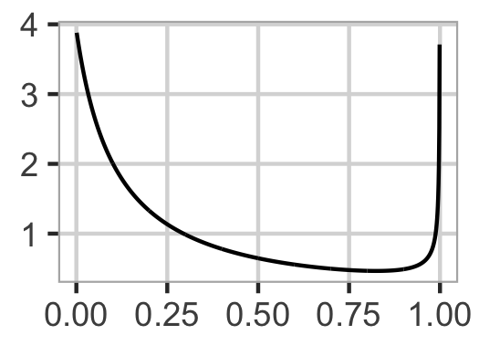
(b) $\pi(\omega)$

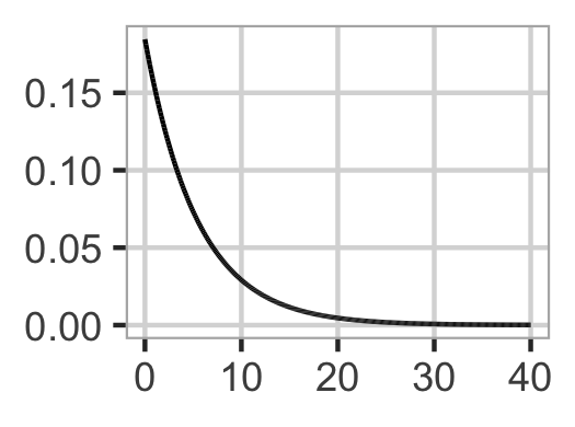
(c) $\pi(d(\omega))$

Figure 2: Model structure and prior for $\omega$ in the random intercept model with 10 individuals in each group and prior median $\omega_{\mathrm{m}}=0.25$. The prior is independent of the number of groups. 2(a)) Tree structure, 2(b)) prior for $\omega$, and 2(c)) prior for distance $d(\omega)$.

The intraclass correlation (ICC) for the random intercept model is given by $\sigma_{\alpha}^{2}/(\sigma_{{\mathrm{R}}}^{2}+\sigma_{\alpha}^{2})$, which equals the weight parameter $\omega$. Thus the shrinkage of the ICC is completely controlled in the construction of the prior and expert knowledge about the ICC can be incorporated directly. Further, $\omega$ can be linked to a generalised version of the coefficient of determination, $R^{2}$, suggested by Gelman and Hill (2007); see Section S3.2 in the Supplementary Materials for details.

We use the R-package RStan (Stan Development Team, 2018b) to perform the inference for the simulation study. We use HD priors from Prior class 2 with shrinkage from PC priors on $\omega$ with hyperparameters $\omega_{\mathrm{m}}=0.25$ (P-HD-25), $\omega_{\mathrm{m}}=0.5$ (P-HD-50) and $\omega_{\mathrm{m}}=0.75$ (P-HD-75), and an HD prior from Prior class 2 where the PC prior is replaced by a Dirichlet prior on $(\omega,1-\omega)$ (P-HD-D) with default hyperparameter. Additional priors are Jeffreys’ prior on the residual variance combined with different priors on the random intercepts variance or standard deviation: the default INLA prior $\text{InvGamma}(1,5\times 10^{-5})$ (P-INLA), $\text{Half-Cauchy}(25)$ (P-HC), and $\text{PC}_{\mathrm{SD}}(3,0.05)$ (P-PC). This gives seven joint priors. Each scenario in the simulation study consists of $500$ datasets which are simulated from the random intercept model for $n_{\mathrm{g}}\in\{5,10,50\}$, and $10$, $50$, or varying number of individuals in each group. We select true values $\omega\in\{0.1,0.25,0.5,0.75,0.9\}$ and select true total variance $V=1$ in every scenario.

We evaluate the performance of the different priors with respect to posterior inference for total variance $V$ and ICC $\omega$. We use the bias of $\log(V)$ and $\text{logit}(\omega)$, calculated using the estimated median minus the true value, and the 80% empirical coverage, found by counting the number of times the true value is contained in the 80% equal-tailed credible interval. We use the same settings for the call to the stan function for all priors and scenarios in the simulation study. RStan reports a divergent transition for each iteration of the MCMC sampler that runs into numerical instabilities (Carpenter et al., 2017). In Figure S3.1 in the Supplementary Materials we report the proportion of datasets that resulted in at most 0.1% divergent transitions for each prior and scenario. This is used as a measure of stability of the inference scheme for each prior, and the dataset and prior combinations causing unstable inference are removed from the study.

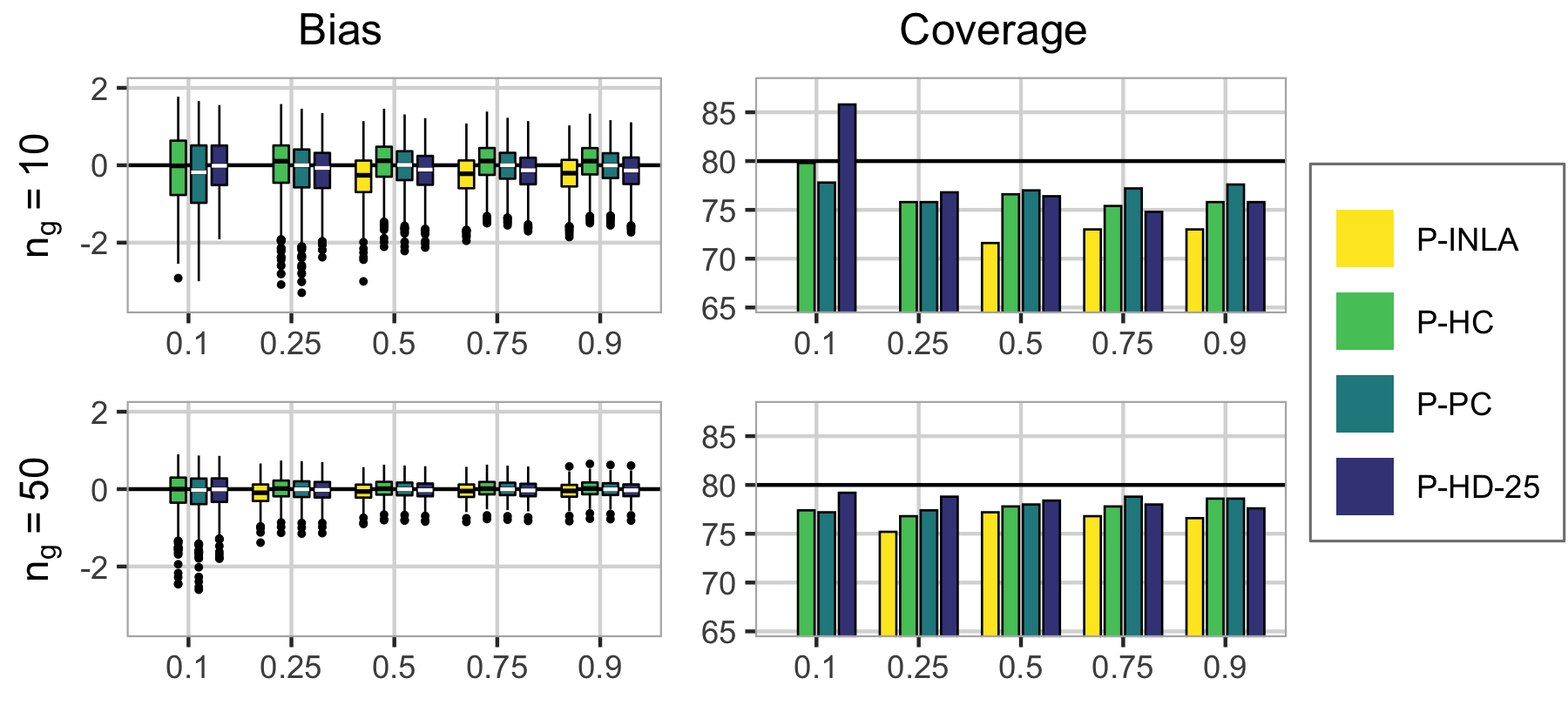
Figure 3: Results for $\text{logit}(\omega)$ for the random intercept simulation study. True value of $\omega$ shown on the $x$-axis, the number of groups is shown on left-hand side, and the group size is 10. Results for P-INLA are only shown when it leads to stable inference.

The results in Figure 3 are for $n_{g}\in\{10,50\}$ and group size $10$, and show that P-HD-25 performs at least as good in terms of bias and coverage of $\text{logit}(\omega)$ as P-INLA, P-HC and P-PC. The magnitude of the bias decreases and the coverage approaches 80% for all four priors when the number of groups increases, which is expected as the amount of information about the parameters in the datasets increases. Figures S3.3–S3.7 in the Supplementary Materials show that the HD priors perform at least as good in terms of bias and coverage for $\text{logit}(\omega)$ as P-INLA, P-HC and P-PC also for the other combinations of the number of groups and group sizes, and that the same conclusions as for $\text{logit}(\omega)$ also holds for $\log(V)$.

Furthermore, Figures S3.3–S3.7 show that the behaviour of the four HD priors is stable with respect to the choice of $\omega_{\mathrm{m}}$ when group size is 10, and that P-HD-D performs worse than P-HD-25, P-HD-50 and P-HD-75 for all values of the true weight except 0.5. For 10 groups with two observations per group, the risk of overfitting is high because low information about the parameters may lead to overestimating the weight parameter and estimating spurious signals in the group effect. In this setting, P-HD-25 leads to overfitting for true weight equal to $0.1$, but underfitting for true weight equal to $0.25$, $0.5$, $0.75$ and $0.9$. P-HD-50, P-HD-75 and P-HD-D result in overfitting for true weight equal to $0.1$ and $0.25$, but underfitting for true weight equal to $0.5$, $0.75$ and $0.9$. See Section S3.4 in the Supplementary Materials for additional details.

Figure S3.1 shows that P-INLA is the only prior that is heavily affected by divergent transitions during the inference for scenarios with 10 or 50 groups. Part of the problem with P-INLA is that it results in a bi-modal posterior for $\sigma_{\alpha}^{2}$; see Figure S3.2. The new HD priors are preferred for the random intercept model due to their intuitive definition, where the structure of the shrinkage is directly available in Figure 2(a), and interpretability of the parametrization which aids prior elicitation.

5.2 Latin square experiment

Consider an experiment where a latin square design (Hinkelmann and Kempthorne, 1994) is used to control for two nuisance sources of noise. For example, a field split into rows and columns where different levels of strength of a new fertilizer is applied to each plot. We assume there are nine possible levels of the treatment so that a $9\times 9$ grid of plots is necessary for a full latin square design. We focus on random effects and exclude fixed effects from the model, and assume that the responses can be modelled by

$$y_{i,j}=\alpha_{i}+\beta_{j}+\gamma_{k[i,j]}+\varepsilon_{i,j},\quad i,j=1,\ldots,9,$$ (5.1)

where $\bm{\alpha}=(\alpha_{1},\ldots,\alpha_{9})\sim\mathcal{N}(\bm{0},\sigma_{\mathrm{r}}^{2}\mathbf{I}_{9})$ is an i.i.d. effect of row, $\bm{\beta}=(\beta_{1},\ldots,\beta_{9})\sim\mathcal{N}_{9}(\bm{0},\sigma_{\mathrm{c}}^{2}\mathbf{I}_{9})$ is an i.i.d. effect of column, $\bm{\gamma}=(\gamma_{1},\ldots,\gamma_{9})$ is the effect of the treatment, $k[i,j]$ denotes the treatment assigned to row $i$ and column $j$, and $\bm{\varepsilon}=(\varepsilon_{1,1},\ldots,\varepsilon_{9,9})\sim\mathcal{N}_{81}(\bm{0},\sigma_{\mathrm{R}}^{2}\mathbf{I}_{81})$ is the residual noise.

We believe that the effect of the treatment is ordered, and that the treatment effect consists of a smooth signal of interest $\bm{\gamma}^{(1)}=(\gamma_{1}^{(1)},\ldots,\gamma_{9}^{(1)})$ and random noise $\bm{\gamma}^{(2)}=(\gamma_{1}^{(2)},\ldots,\gamma_{9}^{(2)})$ we have to control for. The signal is given a second-order random walk model described by $\mathcal{N}_{9}(\bm{0},\sigma_{\mathrm{RW2}}^{2}\mathbf{Q}_{\mathrm{RW2}}^{-1})$, where $\sigma_{\mathrm{RW2}}^{2}$ is the variance and $\mathbf{Q}_{\mathrm{RW2}}^{-1}$ is a slight abuse of notation to describe the intrinsic second-order random walk defined by the precision matrix $\mathbf{Q}_{\mathrm{RW2}}$, and the noise is $\bm{\gamma}^{(2)}\sim\mathcal{N}_{9}(\bm{0},\sigma_{\mathrm{t}}^{2}\mathbf{I}_{9})$. We use the constraints $\sum_{i=1}^{9}\gamma_{i}^{(1)}=0$ and $\sum_{i=1}^{9}i\gamma_{i}^{(1)}=0$ to remove the implicit intercept and linear effect, respectively.

We set the true standard deviations equal, $\sigma_{\mathrm{r}}=\sigma_{\mathrm{c}}=\sigma_{\mathrm{t}}=\sigma_{\mathrm{R}}=0.1$, and let the true effect of treatment be given by $x_{i}=C\left((i-5)^{2}-20/3\right)$, $i=1,\ldots,9$. We entertain three scenarios: $C=0$ for no effect of treatment (S1), $C=0.05$ for medium effect of treatment (S2) and $C=0.2$ for strong effect of treatment (S3). More details on the true treatment effect is included in Section S4.1 in the Supplementary materials, see especially Figure S4.2. We simulate $500$ datasets for each scenario and analyse them with four choices of priors.

The three default priors used are Jeffreys’ prior for $\sigma_{\mathrm{R}}^{2}$ combined with $\text{InvGamma}(1,5\times 10^{-5})$ for $\sigma_{\mathrm{r}}^{2}$, $\sigma_{\mathrm{c}}^{2}$, $\sigma_{\mathrm{t}}^{2}$ and $\sigma_{\mathrm{RW2}}^{2}$ (P-INLA), or $\text{Half-Cauchy}(25)$ (P-HC) or $\text{PC}_{\mathrm{SD}}(3,0.05)$ (P-PC) for $\sigma_{\mathrm{r}}$, $\sigma_{\mathrm{c}}$, $\sigma_{\mathrm{t}}$ and $\sigma_{\mathrm{RW2}}$. We select an HD prior from Prior class 2 using the model structure in Figure 4(a), where the triple split has a Dirichlet prior and the two other splits have PC priors (P-HD-D3). We also decompose the triple split into the two dual splits as shown in Figure 4(b), and use a PC prior on all four splits according to the shrinkage structure in the figure (P-HD-25). In all cases we use default values for the hyperparameters. See Section S2 in the Supplementary Materials for more details on changing a triple split to two dual splits. Figures S4.3, S4.4, S4.10 and S4.11 in the Supplementary Materials show that the implementation of the triple split has little influence on the targets of the analysis.

(a) Original structure

(b) Dual-split structure

Figure 4: Model structure for the latin square simulation study. Gray nodes indicate base models. $(1/3,1/3,1/3)$, $(1/3,2/3)$, and $(1/2,1/2)$ indicates that the base model for the split is a combination of the branches. 4(a)) Original, and 4(b)) alternative structure.

Figure 5: Results from the latin square experiment simulation study.

The targets of the analysis are the posterior distribution of the structured treatment effect $\bm{\gamma}^{(1)}$ and the model fit. The former will be assessed by the continuous rank probability score (CRPS) (Gneiting and Raftery, 2007) and the latter by the leave-one-out log predictive score (LOO-LPS) $-\frac{1}{81}\sum_{i=1}^{81}\log\pi(y_{i}|\bm{y}_{-i})$. The CRPS is a proper scoring rule and given by $\frac{1}{9}\sum_{i=1}^{9}\int_{-\infty}^{\infty}\left(F_{i}(x)-\mathbb{I}(x\geq x_{i})\right)^{2}\mathrm{d}x,$ where $F_{i}$ is the cumulative distribution function for the posterior of $\gamma_{i}^{(1)}$, $x_{i}$ is the true effect of treatment $i$, and $\mathbb{I}$ is the Heaviside function, and is estimated using the procedure of Jordan et al. (2017). We report the proportion of datasets leading to no more than 0.1% divergent transitions for each prior and scenario, and use this as a measure on stability of the inference. These numbers can be seen in Figure S4.5 in the Supplementary Materials, and show that all priors lead to similar stability. The datasets leading to more than 0.1% divergent transitions for one or more priors are removed from the study.

The main results from the simulation study are displayed in Figure 5. Low LOO-LPS indicates good model fit and low CRPS indicates good predictive power for the treatment effect. P-INLA gives a poorer model fit than the other priors, and with respect to predictive power, the HD priors P-HD-D3 and P-HD-25 perform best for S2 and S3. The high predictive power of P-INLA for S1 is due to the fact that P-INLA has a peak at low variance and produces a posterior for the treatment effect with mean closer to zero and lower variance. Overall, the HD prior performs well across all scenarios. The results are stable to changes in the construction of the HD prior and the choice of hyperparameters; see Section S4.2 in the Supplementary Materials for details. The HD priors are preferable to the other priors because of their intuitive parametrization and the interpretability of the a priori assumptions placed on the joint prior of the variance parameters. Further, P-HD-D3 is preferred to P-HD-25 since they perform similar and P-HD-D3 is more intuitive.

6 Case studies: Binomial responses

In this section we study neonatal mortality counts arising from complex surveys through a simulation study, and show how to practically apply the HD priors.

6.1 Background

Neonatal mortality is an important indicator of health and well-being in a country and is included in Goal 3.2 of the Sustainable Development Goals (SDGs) (General Assembly of the United Nations, 2015), and mapping child mortality is an important area of current research (Golding et al., 2017; Wakefield et al., 2018; Li et al., 2019). We define neonatal mortality as the rate of deaths within the first month of life per live birth. An important source of data for neonatal mortality is the nationally-representative household surveys performed by Demographic and Health Surveys (DHS). The survey performed by DHS in 2014 in Kenya targets its 47 counties, which is the relevant administrative level for health policies (Kenya National Bureau of Statistics et al., 2015). The target of the simulation study in Section 6.2 and the analysis in Section 6.3 is the spatial heterogeneity in neonatal mortality in Kenya in the time period 2010 to the time of the survey.

From the survey we can extract the number of live births, $b_{i,j,k}$, and the number of neonatal deaths, $y_{i,j,k}$, in household $k$ in cluster $j$ in county $i$. We also have an indicator $x_{i,j}$ specifying whether the cluster is rural ($0$) or urban ($1$) and each household has an inclusion probability $\pi_{i,j,k}$ of being included in the survey sample. See the Section S5.1 in the Supplementary Materials for more background.

6.2 Simulation study

In this section we use the $n=290$ constituencies shown in Figure 6(a). We assume that $m_{i}=6$ clusters are visited in constituency $i$, $i=1,\ldots,n$, and consider births $b_{i,j}$ and neonatal deaths $y_{i,j}$ in cluster $j$ in constituency $i$. We assume that there are $b_{i,j}=25$ live births in each cluster and the outcomes are simulated according to the model $y_{i,j}|p_{i,j}\sim\text{Binomial}(b_{i,j},p_{i,j})$ for

$$\text{logit}(p_{i,j})=\eta_{i,j}=\mu+u_{i}+v_{i}+\nu_{i,j},\quad j=1,\ldots,m_{i},\ i=1,\ldots,n,$$

where $\mu$ is a joint intercept, $\bm{u}=(u_{1},\ldots,u_{n})$ has a Besag distribution with variance $\sigma_{\mathrm{B}}^{2}$ and a sum-to-zero constraint, $\bm{v}=(v_{1},\ldots,v_{n})\sim\mathcal{N}_{n}(\bm{0},\sigma_{\mathrm{IID}}^{2}\mathbf{I}_{n})$, and $\bm{\nu}=(\nu_{1,1},\ldots,\nu_{n,m_{n}})\sim\mathcal{N}_{M}(\bm{0},\sigma_{\mathrm{C}}^{2}\mathbf{I}_{M})$ with $M=m_{1}+\ldots+m_{n}=6\cdot 290=1740$.

We use the structure for the prior shown in Figure 6(b) to make an HD prior from Prior class 3 with PC priors on all splits according to the base models indicated in the figure (P-HD-25) and an HD prior from Prior class 3 where a Dirichlet prior distributes variance to the three model components (P-HD-D). In all cases, the splits have default hyperparameter values and we select the hyperparameter in the PC prior on total variance, $t=\sigma_{\mathrm{B}}^{2}+\sigma_{\mathrm{IID}}^{2}+\sigma_{\mathrm{C}}^{2}$, so that $\text{P}(t>3)=0.05$. Further, we use $\text{InvGamma}(1,5\times 10^{-5})$ for $\sigma_{\mathrm{B}}^{2}$, $\sigma_{\mathrm{IID}}^{2}$ and $\sigma_{\mathrm{C}}^{2}$ (P-INLA), $\text{Half-Cauchy}(25)$ for $\sigma_{\mathrm{B}}$, $\sigma_{\mathrm{IID}}$ and $\sigma_{\mathrm{C}}$ (P-HC), and the joint prior proposed in Riebler et al. (2016) (P-PC), where $\sigma_{\mathrm{B}}^{2}$ and $\sigma_{\mathrm{IID}}^{2}$ has a PC prior of the type introduced in this paper with $\mathrm{P}(\sigma_{\mathrm{B}}^{2}/(\sigma_{\mathrm{B}}^{2}+\sigma_{\mathrm{IID}}^{2})<0.5)=2/3$ and $\sigma_{\mathrm{C}}^{2}$ is given an independent PC prior $\sigma_{\mathrm{C}}\sim\text{PC}_{\mathrm{SD}}(3,0.05)$.

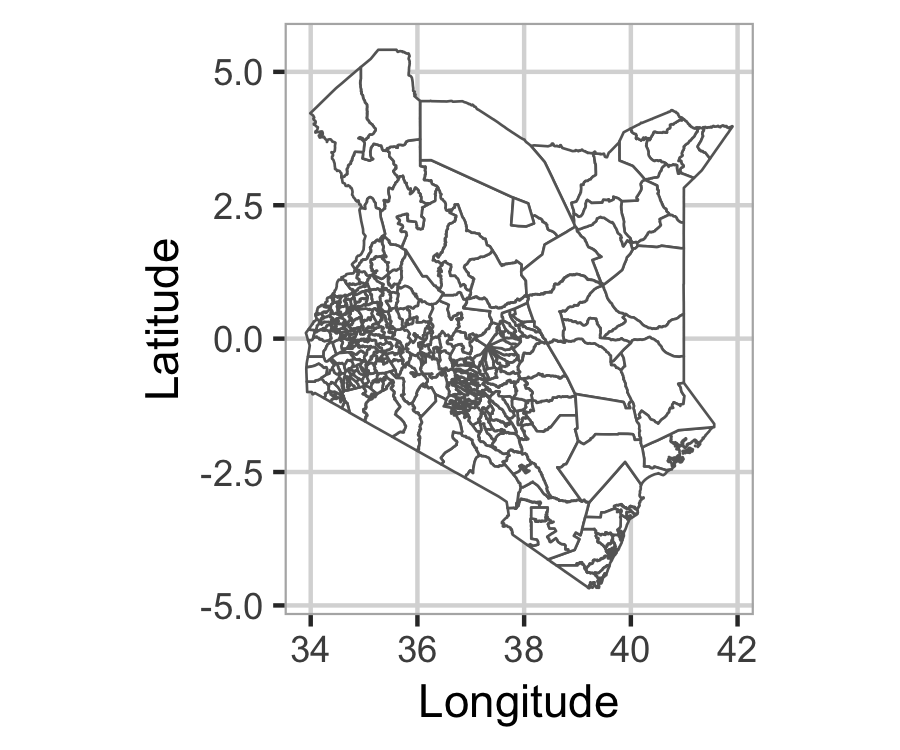
(a) The 290 constituencies of Kenya.

(b) Model structure. Gray nodes indicate base models.

Figure 6: Map and model structure for the Kenya neonatal simulation study.

Based on the final report from the survey (Kenya National Bureau of Statistics et al., 2015) the estimated national level of neonatal mortality is $0.022$ for 2010–2014, and we set $\mu=\text{logit}(0.022)$. Further, we choose $\sigma_{\mathrm{C}}^{2}=0.1$ and create five scenarios by combining this with $\sigma_{\mathrm{IID}}^{2}=\sigma_{\mathrm{B}}^{2}=0$ (S1), $\sigma_{\mathrm{IID}}^{2}=0.4$ and $\sigma_{\mathrm{B}}^{2}=0$ (S2), $\sigma_{\mathrm{IID}}^{2}=\sigma_{\mathrm{B}}^{2}=0.2$ (S3), $\sigma_{\mathrm{IID}}^{2}=0.04$ and $\sigma_{\mathrm{B}}^{2}=0.36$ (S4), and $\sigma_{\mathrm{IID}}^{2}=0$ and $\sigma_{\mathrm{B}}^{2}=0.4$ (S5). We simulate 500 datasets for each scenario. The main targets of the simulation study are the structured part of the spatial heterogeneity through the posterior of $\bm{u}$, the degree of structure in the spatial heterogeneity through $\omega^{(2)}=\sigma_{\mathrm{B}}^{2}(\sigma_{\mathrm{B}}^{2}+\sigma_{\mathrm{IID}}^{2})^{-1}$, and how well the underlying neonatal mortality is estimated through the posterior of the intercept $\mu$. The performance is assessed through the CRPS (see Section 5.2) of $\bm{u}$, the bias of the posterior median of $\omega^{(2)}$, and the bias of the posterior median and the coverage of the 80% equal-tailed credible interval for $\mu$. We use the proportion of datasets leading to at most 0.1% divergent transitions as a measure of stability in the inference, these numbers can be seen in Figure S5.1 in the Supplementary Materials, and show that P-INLA leads to more unstable inference than the others.

Figure 7 shows the main results from the simulation study. We drop datasets that cause more than 0.1% divergent transitions for at least one of the priors from each scenario. All priors have a tendency to overestimate the intercept, with P-INLA doing worse than the others, P-INLA gives close to exact estimates when the true value of $\omega^{(2)}$ is $0$ (in S2) and $1$ (in S5), but performs worse than the other priors for S3 and S4. Figure S5.2 in the Supplementary Materials shows that P-HD-25 performs better than P-HD-D except in S3 where the Dirichlet prior is closest to the truth, and that $\omega^{(1)}$ tends to be underestimated under all the priors. P-HD-25 is preferred because overall it performs at least as good as the other priors P-HC and P-PC, and P-HD-25 is an intuitive and well-behaved prior that takes the hierarchical structure of the model into account.

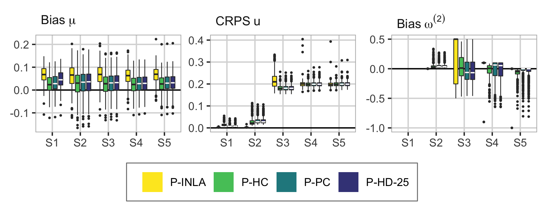
Figure 7: Main results from the Kenya neonatal mortality simulation study. Left to right: bias of the intercept $\mu$, CRPS of $\bm{u}$ and bias of $\omega^{(2)}$. Scenario shown on the x-axes.

6.3 Neonatal mortality in Kenya

This section follows the notation introduced in Section 6.1. The survey consists of 13183 households with one or more live births, distributed over 1593 clusters that are distributed over $n=47$ counties. In total there are 376 deaths among 17664 children. Figure 8(c) shows the counties and the weighted neonatal mortality by the inverse inclusion probabilities, and it is unclear if there is a structured spatial pattern. The neonatal mortality is assumed to follow a survival model with constant hazard through the first month of life, and we use a latent Gaussian model with a binomial likelihood, $y_{i,j,k}|b_{i,j,k},p_{i,j,k}\sim\text{Binomial}(b_{i,j,k},p_{i,j,k}),$ a logit link function, and a linear latent Gaussian model

$$\eta_{i,j,k}=\text{logit}(p_{i,j,k})=\mu+x_{i,j}\beta+u_{i}+v_{i}+\nu_{i,j}+\varepsilon_{i,j,k},$$ (6.1)

where $\mu$ is an overall intercept, $\beta$ is the effect of urban, $\bm{u}$ is a Besag model with variance $\sigma_{11}^{2}$, $\bm{v}$ is a Gaussian i.i.d. effect of county with variance $\sigma_{12}^{2}$, $\bm{\nu}$ is a Gaussian i.i.d. effect of cluster with variance $\sigma_{2}^{2}$, and $\bm{\varepsilon}$ is a Gaussian i.i.d. effect of household with variance $\sigma_{3}^{2}$. In this model, $\bm{u}$ and $\bm{v}$ provide structured and unstructured, respectively, between-county variation, $\bm{\nu}$ provides between-cluster variation, and $\bm{\varepsilon}$ provides within-cluster variation. The Besag effect has a sum-to-zero constraint to make the overall intercept identifiable. The random effects of cluster and household are necessary to account for the dependence induced between sampled households due to the clustering in the sampling design. We assume that there is no difference between the effect of urbanicity between different counties.

The model has four variance parameters that must be assigned a joint prior. The first step is to choose the tree structure. For simplicity’s sake, the alternatives to the full model (6.1) we would entertain are first $\eta_{i,j,k}=\mu+x_{i,j}\beta+v_{i}$, then we would add $u_{i}$, so $\nu_{i,j}$, and at last $\varepsilon_{i,j,k}$. We prefer coarser unstructured effects over finer unstructured effects since we would like to explain the data at a coarser level if possible, and we prefer the unstructured spatial effect over the structured spatial effect since we want to reduce the risk of estimating spurious spatial signals. This gives the nested tree structure in Figure 8(a) where the household effect, cluster effect and Besag effect are sequentially split off from the total latent variance. We construct an HD prior based on the tree structure with PC priors with default hyperparameter values for the splits, and induce shrinkage on the total latent variance as in Prior class 3 with a PC prior where $\mathrm{P}(\text{Total variance}>11.296)=0.05$. This corresponds to a priori equal-tailed 90% credible interval of $(0.1,10)$ for the effect of the random effects on the odds-ratio, $\exp(u_{i}+v_{i}+\nu_{i,j}+\varepsilon_{i,j,k})$. This allows for high variation in the data and is used because the data is observed at the household level. The splits in Figure 8(a) are given PC priors with default hyperparameters and bases models as indicated in the figure.

(a) Model structure.

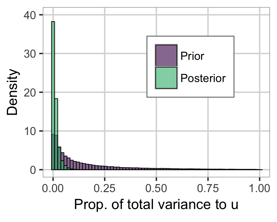
(b) Variance of $\bm{u}$ relative to total variance.

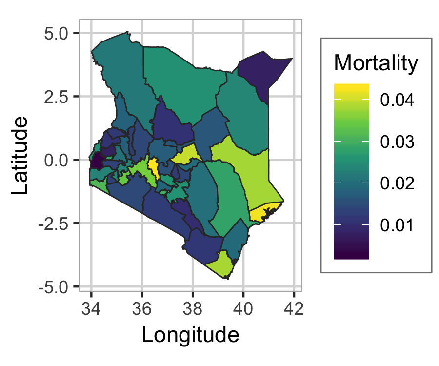
(c) Weighted average of neonatal mortality.

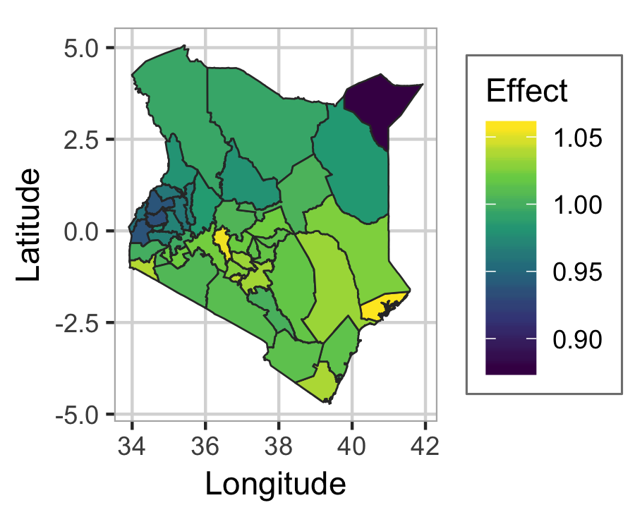
(d) Posterior median of $e^{\bm{u}}$.

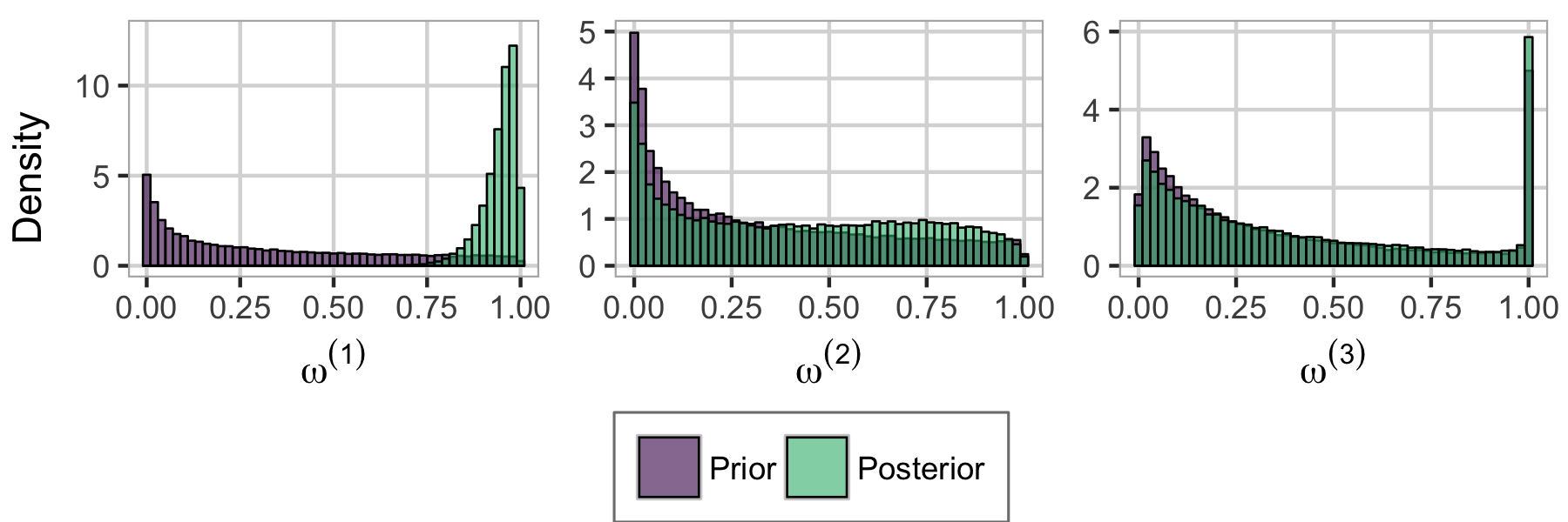
(e) The priors and posteriors for the proportion of household variance to total variance of the random effects $\omega^{(1)}$, the proportion of cluster variance to cluster- and household-level variance $\omega^{(2)}$, and the proportion of structured spatial variance to total between-county variance $\omega^{(3)}$.

Figure 8: Description of model structure, map of observed mortality, and results for neonatal mortality in Kenya.

The model is parameterized by total standard deviation $\sigma_{\mathrm{T}}$, and proportion of household variance to total variance of the random effects $\omega^{(1)}$, proportion of cluster variance to the sum of cluster and county variance $\omega^{(2)}$, and the proportion of structured spatial variance to county variance $\omega^{(3)}$. The priors and posteriors of the proportions $\omega^{(1)}$, $\omega^{(2)}$ and $\omega^{(3)}$ are shown in Figure 8(e). The total standard deviation has a posterior median of $1.47$, and the prior and posterior can be seen in Figure S5.3 in the Supplementary Materials. The results show that the data only weakly informs about the proportion of structured to unstructured spatial effects, which indicates that the data provide no strong evidence in favor of or against a structured spatial effect. Also the posterior of $\omega^{(2)}$ is similar to the prior, but there is a strong signal in the posterior of $\omega^{(1)}$ that there is non-negligible household-level dependence. A plausible explanation for the weak signals in $\omega^{(2)}$ and $\omega^{(3)}$ is that there is substantial noise coming from high variance in the household-level random effect and weak information from the Binomial likelihood due to few successes and few numbers of trials.

As shown in Figure 8(b) the proportion of the total latent variance attributed to the structured spatial effect is low and the posterior median is 0.56%. The estimated spatial effect in Figure 8(d) only explains a small part of the variation seen in the observed data in Figure 8(c). One should be careful to draw conclusions about spatial variation based on Figure 8(d) because the data is only weakly informative about the split between the structured and the unstructured spatial random effects $\omega^{(3)}$, and there is only weak evidence for the spatial effect being different from 0 as shown in Figure S5.5 in the Supplementary Materials. The fact that the comparisons of priors and posteriors for $\omega^{(2)}$ and $\omega^{(3)}$ directly informs about the weak signal in the data is an advantage of the parametrization through proportions of variance, and a strong argument for setting priors on $\omega^{(2)}$ and $\omega^{(3)}$ rather than independent priors on the variance of each effect since the resulting posteriors for $\omega^{(2)}$ and $\omega^{(3)}$ are strongly dependent on the resulting implicit priors for $\omega^{(2)}$ and $\omega^{(3)}$.

One could argue for other splits in the tree in Figure 8(a) such as preferring finer level effects to coarser level effects because one does not want to estimate spurious cluster-level or county-level effects, but the key point of this application is that it is easy to set up the prior based on a priori assumptions and the assumptions are available to other scientists at a glance. With the traditional approach of independent priors, the resulting prior on the total variance of the random effects and the distribution of this total variance to the different random effects is obfuscated. Furthermore, if expert knowledge indicates that stronger relative shrinkage of the variances than the default setting is needed, the medians of the conditional priors for $\omega^{(1)}$, $\omega^{(2)}$ and $\omega^{(3)}$ can be reduced.

7 Discussion

Independent priors for the variance parameters in a BHM result in an implicit prior on the total variance of the random effects, $t$, and the attribution of $t$ to the random effects. Additive models are typically built in a modular fashion, but these implict priors are not consistent with respect to adding or removing random effects. In the case of Gaussian responses, both the prior for $t$ and the prior for $t$ relative to the size of the residual variance change. The proposed HD priors overcomes these shortcomings, and respect the defined model structure and are consistent for $t$ and the attribution of $t$ to the different random effects for different selections of random effects.

The HD priors admit a visual representation through trees that allow transparent communication of the assumptions made in constructing the priors and facilitate discussion around the assumptions. The tree clearly specifices where shrinkage has been applied, and in some cases lead to more intuitive parametrization that is more suitable for elicitation of priors. For the random intercept model, the tree-based hierarchical variance decomposition leads to a parameterisation in terms of $t$ and the ICC. A prior on these parameters is more interpretable than separate priors on the group variance and individual variance, which obfuscates the joint effect of the priors. The increased interpretability of joint priors compared to independent priors addresses concerns raised about transparency for point processes where prior sensitivity is a major concern (Sørbye et al., 2018).

The mix of robust PC priors for shrinkage and simple Dirichlet priors for expressing ignorance, allows principled priors that respect the relative complexity of the random effects when shrinkage is necessary, and intuitive exchangeability when no random effects are preferred or no model structure is apparent. The simulation studies show that this approach performs better than a completely unstructured approach with a Dirichlet prior attributing $t$ to the different random effects, but that Dirichlet priors perform well for subgroups of the random effects where there is no nested structure or difference in complexity.

HD priors with default settings for the hyperparameters performs well, but there are corner cases like no treatment effect in the latin square experiment and no structured spatial effect for the binomial data, which are best handled by the default INLA prior. However, this prior has a peak in the prior distribution for low variances and generally performs surprisingly bad. The HD priors perform comparable to component-wise PC priors and separate half-cauchy priors for the marginal variances. The main benefit of the HD priors over other default priors is their combination of intuitive graphical representation with robust inference that behaves well across a range of different scenarios.

The calculation of PC priors is more complex in the context of correlation parameters, but multivariate PC priors have been developed for more complex random effects such as autoregressive processes (Sørbye and Rue, 2017) and spatial Matérn models (Fuglstad et al., 2019). These can be integrated into the HD prior framework by first defining priors on the correlation parameters, and then constructing the joint prior for the variance parameters with the correlation parameters fixed to reasonable values. This follows the pragmatic mindset of Assumption 2 of producing priors that are computationally feasible, intuitive and practically useful.

A key focus for future work is to exploit sparsity in the precision matrices of the random effects. This is important when shrinkage is desired through PC priors because many models such as random walks, Besag models, and Gaussian random fields (Lindgren et al., 2011) have dense covariance matrices, but can be expressed through sparse precision matrices. Assume that the total variance is split between random effects with sparse precision matrices $\mathbf{Q}_{1}$ and $\mathbf{Q}_{2}$, where $\mathbf{Q}_{1}$ corresponds to the base model. Let $0<\omega<1$, then the KLD used in Theorem 1 consists of the trace of $\mathbf{Q}_{1}[(1-\omega)\mathbf{Q}_{1}^{-1}+\omega\mathbf{Q}_{2}^{-1}]$, which can be computed quickly through the techniques in Rue and Held (2010, Section 12.1.7.10), and the determinant $\det[\mathbf{Q}_{1}[(1-\omega)\mathbf{Q}_{1}^{-1}+\omega\mathbf{Q}_{2}^{-1}]=\det[(1-\omega)\mathbf{Q}_{2}+\omega\mathbf{Q}_{1}](\det[\mathbf{Q}_{2}])^{-1}$, which can be computed quickly through Cholesky factorizations.

We aim to further broaden the advantages of the HD priors in the future by constructing a joint prior for the variance parameters and the fixed effects. However, this will require re-thinking of the concept of total latent variance as it is the values of the coefficients of the fixed effects and not their variance that determines the amount of variance they explain. Instead of starting with the concept of marginal variances, it is natural to begin with the classical concept of explained variance and use ideas from block-wise g-priors (Som et al., 2014) to distribute variance inside a group of covariates. In a multilevel model this would connect the attribution of explained variance to different levels to generalised coefficients of determinations. Additionally, towards non-parametric regression by including a combination of a linear effect of a covariate and a smooth effect of a covariate, and explicitly putting a prior on the degree of non-linearity (Simpson et al., 2017, Section 7). However, there are still open questions and this addition is outside the scope of this paper.

The choice of tree structure for HD priors should be guided by the application at hand, for example, by considering the relative complexity of the random effects. When expert knowledge is available, the default values for the hyperparameters should be replaced by values elicited based on expert knowledge. We believe that the advantages of the HD priors over independent priors mean that they should be used as the default option in software for Bayesian analysis. However, it is necessary to make the selection and computation of HD prior for a specific problem easier for analysts. We plan to address this by providing a separate R package, which is compatible with INLA, that provides a graphical user interface for selecting the tree structure and selecting priors for the splits, and has the option to pre-compute priors for use in RStan. This will allow analysts to experiment with different a priori assumptions and produce graphical figures that summarize their assumptions and can be communicated to fellow scientists. This will encourage transparancy and clarity in a priori assumptions in the scientific community.

Appendix A: Supplementary materials

S1 Proofs

S1.1 Theorem 3.1

Theorem 1 (Prior for the case $N=2$).

Let $\bm{u}_{1}$ and $\bm{u}_{2}$ be random effects of an LGM that enter the linear predictor through $\mathbf{A}_{1}\bm{u}_{1}\sim\mathcal{N}_{n}(\bm{0},\sigma_{1}^{2}\tilde{\Sigma}_{1})$ and $\mathbf{A}_{2}\bm{u}_{2}\sim\mathcal{N}_{n}(\bm{0},\sigma_{2}^{2}\tilde{\Sigma}_{2})$. Assume that $\tilde{\Sigma}_{1}+\tilde{\Sigma}_{2}$ is non-singular. Let $\omega=\sigma_{2}^{2}/(\sigma_{1}^{2}+\sigma_{2}^{2})$ and $\Sigma(w)=(1-\omega)\tilde{\Sigma}_{1}+\omega\tilde{\Sigma}_{2}$. Then the distance from the base model $\Sigma(\omega_{0})$ to the alternative model $\Sigma(\omega)$ is given by $d(\omega)=\sqrt{\mathrm{tr}(\Sigma(\omega_{0})^{-1}\Sigma(\omega))-n-\log|\Sigma(\omega_{0})^{-1}\Sigma(\omega)|}$ for $0\leq\omega_{0}\leq 1$.

The PC prior for $\omega$ with base model $\omega_{0}=0$ is

$$\pi(\omega)=\begin{cases}\frac{\lambda\left|d^{\prime}\left(\omega\right)\right|}{1-\exp(-\lambda d(1))}\exp\left(-\lambda d\left(\omega\right)\right),&\text{$0<w<1$, $\tilde{\Sigma}_{1}$ non-singular},\\ \frac{\lambda}{2\sqrt{\omega}(1-\exp(-\lambda))}\exp(-\lambda\sqrt{\omega}),&\text{$0<\omega<1$, $\tilde{\Sigma}_{1}$ singular},\end{cases}$$

where $\lambda>0$ is the hyperparameter. We suggest to set $\lambda$ so that the median is $\omega_{\mathrm{m}}=0.25$.

For base model $0<\omega_{0}<1$, the PC prior whose median is equal to $\omega_{0}$ is

$$\pi(\omega)=\begin{cases}\frac{\lambda\left|d^{\prime}\left(\omega\right)\right|}{2[1-\exp(-\lambda d(0))]}\exp\left(-\lambda d\left(\omega\right)\right),&0<\omega<\omega_{0},\\ \frac{\lambda\left|d^{\prime}\left(\omega\right)\right|}{2[1-\exp(-\lambda d(1))]}\exp\left(-\lambda d\left(\omega\right)\right),&\omega_{0}<\omega<1,\par\end{cases}$$

where $\lambda>0$ is a hyperparameter. We suggest to set $\lambda$ so that

$$\mathrm{P}(\mathrm{logit}(1/4)+\mathrm{logit}(\omega_{0})<\mathrm{logit}(\omega)<\mathrm{logit}(\omega_{0})+\mathrm{logit}(3/4))=1/2.$$

Base model equal to $\omega_{0}=1$ follows directly by reversing the roles of $\bm{u}_{1}$ and $\bm{u}_{2}$.

Proof:
First, note that since $\tilde{\Sigma}_{1}$ and $\tilde{\Sigma}_{2}$ are positive semi-definite and $\tilde{\Sigma}_{1}+\tilde{\Sigma}_{2}$ is non-singular, $\Sigma(\omega)=(1-\omega)\tilde{\Sigma}_{1}+\omega\tilde{\Sigma}_{2}$ is positive definite for $0<\omega<1$. This follows from the fact that $\tilde{\Sigma}_{1}+\tilde{\Sigma}_{2}$ is non-singular means that $\bm{v}^{\mathrm{T}}(\tilde{\Sigma}_{1}+\tilde{\Sigma}_{2})\bm{v}\neq 0$ for $\bm{v}\in\mathbb{R}^{n}$ and $\bm{v}\neq\bm{0}$, where $n$ is the dimension of $\tilde{\Sigma}_{1}$, which implies that either $\bm{v}^{\mathrm{T}}\tilde{\Sigma}_{1}\bm{v}>0$ or $\bm{v}^{\mathrm{T}}\tilde{\Sigma}_{2}\bm{v}>0$ for each $\bm{v}\neq\bm{0}$ so that $\bm{v}^{\mathrm{T}}[(1-\omega)\tilde{\Sigma}_{1}+\omega\tilde{\Sigma}_{2}]\bm{v}>0$ for $\bm{v}\in\mathbb{R}^{n}$ and $\bm{v}\neq\bm{0}$.

The proof of the theorem is split into three cases.

Case 1: $\omega_{0}=0$ and $\tilde{\Sigma}_{1}$ is non-singular

The Kullback-Leibler divergence (KLD) from $\mathcal{N}_{n}(\bm{0},\Sigma(\omega))$ to $\mathcal{N}_{n}(\bm{0},\tilde{\Sigma}_{1})$ is given by $\text{KLD}(\omega)=0.5(\text{tr}(\tilde{\Sigma}_{1}^{-1}\Sigma(\omega))-n-\log(|\tilde{\Sigma}_{1}^{-1}\Sigma(\omega)|))$, where tr denotes the trace of the matrix, and $\mathrm{KLD}(\omega)$ is finite for $0\leq\omega<1$ since the KLD between two non-singular multivariate Gaussian distributions is finite. Thus a distance can be defined through

$$d(\omega)=\sqrt{\text{tr}(\tilde{\Sigma}_{1}^{-1}\Sigma(\omega))-n-\log(|\tilde{\Sigma}_{1}^{-1}\Sigma(\omega)|)},\quad 0\leq\omega<1,$$ (S1.1)

and we follow Simpson et al. (2017) and use an exponential distribution on the distance so that $\pi(d)=\lambda\exp(-\lambda d)(1-\exp(-\lambda d(1)))^{-1}$, $0<d<d(1)$, where $\lambda>0$, and the possibly truncated density is normalized by $(1-\exp(-\lambda d(1)))$. A change of variables gives

$$\pi(\omega)=\frac{\lambda|d^{\prime}(\omega)|}{1-\exp(-\lambda d(1))}\exp(-\lambda d(\omega)),\quad 0<\omega<1.$$ (S1.2)

∎

Case 2: $\omega_{0}=0$ and $\tilde{\Sigma}_{1}$ is singular

If $\tilde{\Sigma}_{1}$ is singular and $\Sigma(\omega)$, $0<\omega<1$, is non-singular, the distance $d(\omega)$ given in Equation (S1.1) is infinite for all $0<\omega<1$ and the direct approach for constructing the prior is not possible. We change the notation to $d(\omega;\omega_{0})$ to make the dependence on the base model explicit. For any base model $\omega_{0}>0$, $d(\omega;\omega_{0})$ is finite for $\omega_{0}\leq\omega<1$, and the prior can be constructed as for Case 1. The distance $d(\omega;\omega_{0})$ is scaled by $\lambda$ in Equation (S1.2) and we seek an expression $\lambda(\omega_{0})$ so that $\lambda(\omega_{0})d(\omega;\omega_{0})$ remains finite for all $\omega_{0}\leq\omega<1$ when $\omega_{0}\rightarrow 0^{+}$.

Since $\tilde{\Sigma}_{1}+\tilde{\Sigma}_{2}$ is positive definite, there exist an $n\times n$ matrix $\mathbf{P}$ so that

$$\mathbf{P}(\tilde{\Sigma}_{1}+\tilde{\Sigma}_{2})\mathbf{P}^{\mathrm{T}}=\mathbf{I}.$$

This corresponds to a linear transformation of the Gaussian distributions that results in covariance matrices $\mathbf{S}_{1}=\mathbf{P}\tilde{\Sigma}_{1}\mathbf{P}^{\mathrm{T}}$ and $\mathbf{S}_{2}=\mathbf{P}\tilde{\Sigma}_{2}\mathbf{P}^{\mathrm{T}}$. The KLD is invariant to a linear transformation of the variables and the distance in Equation (S1.1) can be calculated by

$$d(\omega;\omega_{0})^{2}=\text{tr}(\mathbf{S}(\omega_{0})^{-1}\mathbf{S}(\omega))-n-\log(|\mathbf{S}(\omega_{0})^{-1}\mathbf{S}(\omega)|),$$

where

$$\mathbf{S}(\omega)=(1-\omega)\mathbf{S}_{1}+\omega\mathbf{S}_{2}=\omega(\mathbf{S}_{1}+\mathbf{S}_{2})+(1-2\omega)\mathbf{S}_{2}=\omega\mathbf{I}+(1-2\omega)\mathbf{S}_{1},$$

since $\mathbf{S}_{1}+\mathbf{S}_{2}=\mathbf{I}$.

$\mathbf{S}_{1}$ is symmetric and can be diagonalized so that $\mathbf{S}_{1}=\sum_{i=1}^{n}\lambda_{i}\bm{v}_{i}\bm{v}_{i}^{\mathrm{T}}$. This gives

$$\mathbf{S}(\omega)=\sum_{i=1}^{n}[(1-2\omega)\lambda_{i}+\omega]\bm{v}_{i}\bm{v}_{i}^{\mathrm{T}}$$

so that

$$\mathbf{S}(\omega_{0})^{-1}\mathbf{S}(\omega)=\sum_{i=1}^{n}\frac{[(1-2\omega)\lambda_{i}+\omega]}{[(1-2\omega_{0})\lambda_{i}+\omega_{0}]}\bm{v}_{i}\bm{v}_{i}^{\mathrm{T}}.$$

Thus the distance is given by

$$d(\omega;\omega_{0})^{2}=\sum_{i=1}^{n}\frac{[(1-2\omega)\lambda_{i}+\omega]}{[(1-2\omega_{0})\lambda_{i}+\omega_{0}]}-n-\sum_{i=1}^{n}\log\left(\frac{[(1-2\omega)\lambda_{i}+\omega]}{[(1-2\omega_{0})\lambda_{i}+\omega_{0}]}\right).$$

Let $l$ be the rank deficency of $\tilde{\Sigma}_{1}$ and assume that the eigenvalues of $\mathbf{S}_{1}$ are sorted from largest to smallest, then $\lambda_{i}>0$ for $i=1,\ldots,n-l$ and $\lambda_{i}=0$ for $i=n-l+1,\ldots,n$, and the distance can be written as

$$d(\omega;\omega_{0})^{2}=l\left(\frac{w}{\omega_{0}}-\log\left(\frac{\omega}{\omega_{0}}\right)\right) +\sum_{i=1}^{n-l}\frac{[(1-2\omega)\lambda_{i}+\omega]}{[(1-2\omega_{0})\lambda_{i}+\omega_{0}]}$$

$$-n-\sum_{i=1}^{n-l}\log\left(\frac{[(1-2\omega)\lambda_{i}+\omega]}{[(1-2\omega_{0})\lambda_{i}+\omega_{0}]}\right).$$

The first term blows up as $\omega_{0}$ tends to zero, whereas the latter terms converges to a finite value. We introduce the scaled distance

$$\tilde{d}(\omega;\omega_{0})^{2}=\omega_{0}d(\omega;\omega_{0})^{2}=l\left(\omega-\omega_{0}\log\left(\frac{\omega}{\omega_{0}}\right)\right)+\omega_{0}C(\omega_{0}),$$

where $C(\omega_{0})=\mathcal{O}(1)$ as $\omega_{0}\rightarrow 0^{+}$, and define $\tilde{d}(\omega;0)=\lim_{\omega_{0}\rightarrow 0^{+}}\sqrt{\omega_{0}}d(\omega;\omega_{0})=\sqrt{lw}.$

Thus by letting $\lambda(\omega_{0})=\sqrt{\omega_{0}/l}\tilde{\lambda}$, we find the density

$$\pi(\omega)=\frac{\tilde{\lambda}}{2\sqrt{\omega}(1-\exp(-\tilde{\lambda}))}\exp(-\tilde{\lambda}\sqrt{\omega}),\quad 0<\omega<1,$$ (S1.3)

as $\omega_{0}\rightarrow 0^{+}$.

∎

Case 3: $0<\omega_{0}<1$

This case proceeds like Case 1 for $0\leq\omega<\omega_{0}$ and for $\omega_{0}<\omega<1$. On each side of $\omega_{0}$ we get a similar expression as in Equation (S1.2). If we want to place the median at $\omega_{0}$ we must place $1/2$ probability on each side of $\omega_{0}$ by introducing factors of $1/2$ in the expressions. The density becomes

$$\pi(\omega)=\begin{cases}\frac{\lambda\left|d^{\prime}\left(\omega\right)\right|}{2(1-\exp(-\lambda d(0)))}\exp\left(-\lambda d\left(\omega\right)\right),&0<\omega<\omega_{0},\\ \frac{\lambda\left|d^{\prime}\left(\omega\right)\right|}{2(1-\exp(-\lambda d(1)))}\exp\left(-\lambda d\left(\omega\right)\right),&\omega_{0}<\omega<1,\par\end{cases}$$

where $(1-\exp(-\lambda d(0)))$ makes sure the density in $0<\omega<\omega_{0}$ integrates to $1/2$ and $(1-\exp(-\lambda d(1)))$ makes sure the density in $\omega_{0}<\omega<1$ integrates to $1/2$. ∎

S2 Multivariate PC priors for ignorance

The PC prior framework can be applied directly to dual splits since distance can be defined as a function of a single parameter. However, the PC prior framework does not translate to a general approach for distances that are functions of multiple parameters without further assumptions (Simpson et al., 2017, Section 6). Consider a split with $K>2$ branches, and denote the proportion of variances assigned to each branch as $\bm{\omega}=(\omega_{1},\ldots,\omega_{K})$. Assume that the base model for the split is equal apportion of variance into the branches. Then the following procedure can be applied to replace the split with a sequence of dual splits.

Assumption 3 (Turn a multi-split into dual splits).

Consider a split in the tree structure that has $K>2$ branches and assume that the variance in each branch is $\tilde{\sigma}_{i}^{2}$, for $i=1,\ldots,K$. We sequentially split out random effect 1, 2, and so on, through $K-1$ dual splits. The proportion of variance assigned to random effect $i$ of the total variance $\sum_{j=i}^{K}\tilde{\sigma}_{j}^{2}$ is $\omega^{(i)}=\tilde{\sigma}_{i}^{2}/\sum_{j=i}^{K}\tilde{\sigma}_{j}^{2}$ for $i=1,\ldots,K-1$. The base models are $\omega_{0}^{(i)}=1/(K+1-i)$, and ensures that conditioning on the base models results in a proportion of $1/K$ of the total variance to each child node.

The priors for each dual split can be precomputed before inference. The prior depends on the ordering of the $K-1$ dual splits, but when the hyperparameters are set according to the suggested values for dual splits in the main article, we do not expect the ordering of the child nodes within each multisplit to greatly affect inference because the conditional priors are weakly informative in the sense that they put most mass around the base models, but also ensure that large deviations from the base model are plausible. The base models are chosen so that the variance is split equally between the child nodes.

S3 Gaussian responses: Random intercept model

In this section we include additional background, theory and results for the random intercept model simulation study from Section 5.1 in the main article.

S3.1 Additional background

The random intercept model is given by

$$y_{i,j}=\alpha_{i}+\varepsilon_{i,j},\quad j=1,\dots,n_{i},\,i=1,\dots,n_{\mathrm{g}},\,N=\sum_{i=1}^{n_{\mathrm{g}}}n_{i},$$ (S3.1)

where $y_{i,j}$ is the $j$-th observation in group $i$, $\bm{\alpha}=(\alpha_{1}\dots,\alpha_{n_{\mathrm{g}}})^{\mathrm{T}}\sim\mathcal{N}_{n_{\mathrm{g}}}(\bm{0},\sigma_{\alpha}^{2}\mathbf{I}_{n_{\mathrm{g}}})$ is a vector with the random intercepts (group effect), and $\bm{\varepsilon}=(\varepsilon_{1,1},\varepsilon_{1,2},\dots,\varepsilon_{n_{g},n_{n_{\mathrm{g}}}})^{\mathrm{T}}\sim\mathcal{N}_{N}(\bm{0},\sigma_{\mathrm{R}}^{2}\mathbf{I}_{N})$ is the residual noise (individual effect). We denote the $N$-dimensional vector of observations $\bm{y}=(y_{1,1},y_{1,2},\dots,y_{n_{\mathrm{g}},n_{n_{\mathrm{g}}}})^{\mathrm{T}}$ and let $\mathbf{A}$ be a block matrix of size $N\times n_{\mathrm{g}}$ connecting the correct entries of $\bm{\alpha}$ to each observation in $\bm{y}$. Reparameterizing the model with total variance $V=\sigma_{\mathrm{R}}^{2}+\sigma_{\alpha}^{2}$ and $\omega=\sigma_{\alpha}^{2}/V$, the model can be written in vector form as

$$\bm{y}=\sqrt{V}\left(\sqrt{\omega}\mathbf{A}\bm{\alpha}+\sqrt{1-\omega}\bm{\varepsilon}\right),\ (\bm{\alpha},\bm{\varepsilon})\sim\mathcal{N}_{n_{\mathrm{g}}+N}(\bm{0},\mathbf{I}_{n_{\mathrm{g}}+N}).$$ (S3.2)

We use the R package RStan (Stan Development Team, 2018b) to perform the inference for all the three simulation studies in the paper. More specifically, we use the function stan from this package, where we use the following settings for the random intercept model simulation study: burn-in of length 25 000, total sample length of 125 000 (i.e., 100 000 samples after burn-in), one chain, we thin the chain to every fifth sample, initialize all parameters to zero, and we set the value adapt_delta to 0.95. adapt_delta is the average proposal acceptance probability Stan aims for during the adaption (burn-in) period, and a larger value will give a smaller step size (Stan Development Team, 2018a). For all other inputs we use the default values. We ran the simulation study on a computing cluster, where the full study runs in between a day and a week, depending on the available memory on the cluster.

RStan reports a divergent transition for each iteration of the MCMC sampler that runs into numerical instabilities (Carpenter et al., 2017). The divergent transitions are typically caused by an inappropriately large step size in the sampler or a poorly parameterized model, and may indicate that the results are biased since the sampler had trouble exploring the posterior (Stan Development Team, 2018a). It is difficult to completely avoid divergent transitions across all datasets, but to avoid reporting biased results, we removed dataset and prior combinations that resulted in 0.1% or more divergent transitions during the inference for $n_{\mathrm{g}}=10$ or $50$. For $n_{\mathrm{g}}=5$ we remove the dataset from the study if at least one prior results in too many divergent transitions. We report the proportion of datasets that resulted in at most 0.1% divergent transitions for each prior and scenario and use this as a measure of stability of the inference scheme for each prior.

S3.2 Connection to $R^{2}$

The coefficient of determination, commonly known as $R^{2}$, is a measure on how much of the data variance is explained by a given linear regression model (Gelman and Hill, 2007). In frequentistic statistics, the $R^{2}$ is used to assess model fit by comparing the variance in the residuals to the variance in the data. Gelman and Hill (2007) generalise the $R^{2}$ to also make sense for multilevel models, such as the random intercept model. In this approach the $R^{2}$ is computed at each level of the model, which means we can assess the model fit at each level. In the case of the random intercept model, we have two levels in the model. The classical $R^{2}$ can be written as

$$R^{2}=1-\frac{\sum_{i=1}^{N}(y_{i}-\hat{y}_{i})^{2}}{\sum_{i=1}^{N}(y_{i}-\bar{y})^{2}}$$ (S3.3)

where $y_{i}$, $i=1,\dots,N$, are observations, $\bar{y}=N^{-1}\sum_{i=1}^{N}y_{i}$, and $\hat{y}_{i}$ are the fitted values. Originally, the $R^{2}$ compares the model fit of any given linear regression model with covariates to a regression model with only an intercept. Gelman and Hill (2007) define the generalised $R^{2}$ at each level $k$ in the model to be a comparison of the errors $\varepsilon_{i}^{(k)}$ at level $k$ and the total linear predictor $\eta_{i}^{(k)}$ at the same level of the model. The total linear predictor $\eta_{i}^{(k)}$ is the covariates and predictors at level $k$ in addition to the errors at the level, which means that $\eta_{i}^{(k)}\geq\varepsilon_{i}^{(k)}$ for all $k$. We write the generalised $R^{2}$ as

$$R_{\text{gen}}^{2,(k)}=1-\frac{\text{E}\left(\frac{1}{n_{k}}\sum_{i}\left(\varepsilon_{i}^{(k)}-\bar{\varepsilon}_{i}^{(k)}\right)^{2}\right)}{\text{E}\left(\frac{1}{n_{k}}\sum_{i}\left(\eta_{i}^{(k)}-\bar{\eta}_{i}^{(k)}\right)^{2}\right)}$$ (S3.4)

where $n_{k}$ is the number of observations/groups at level $k$. The random intercept model has two levels, so $k\in\{1,2\}$. In the main article we have standardised the data and omitted the intercept from the random intercept model we use, and we have no covariates. This means that $\varepsilon_{i}^{(1)}=\varepsilon_{i}$, $\eta_{i}^{(1)}=y_{i}$, $\varepsilon_{i}^{(2)}=\alpha_{i}$ and $\eta_{i}^{(2)}=\alpha_{i}$, and we have that

$$\text{E}\left(\frac{1}{n_{\mathrm{g}}}\sum_{i}(\alpha_{i}-\bar{\alpha}_{i})^{2}\right) \stackrel{{\scriptstyle n_{\mathrm{g}}\to\infty}}{{=}}\text{E}\left(\text{Var}\left(\bm{\alpha}\right)\right)=\sigma_{\alpha}^{2},$$ (S3.5)

$$\text{E}\left(\frac{1}{N}\sum_{i}(\varepsilon_{i}-\bar{\varepsilon}_{i})^{2}\right) \stackrel{{\scriptstyle N\to\infty}}{{=}}\text{E}\left(\text{Var}\left(\bm{\varepsilon}\right)\right)=\sigma_{\mathrm{R}}^{2},$$ (S3.6)

$$\text{E}\left(\frac{1}{N}\sum_{i}(y_{i}-\bar{y}_{i})^{2}\right) \stackrel{{\scriptstyle N\to\infty}}{{=}}\text{E}\left(\text{Var}\left(\bm{y}\right)\right)=\sigma_{\alpha}^{2}+\sigma_{\mathrm{R}}^{2}.$$ (S3.7)

The generalised $R^{2}$ at the group level ($k=2$) for our model is zero (in the limit $n_{\mathrm{g}}\to\infty$), which makes sense as there is nothing more in the linear predictor than the errors at the lowest level when we have no covariates in the model. For the data level, the generalised $R^{2}$ is given by $1-\sigma_{\mathrm{R}}^{2}/(\sigma_{\alpha}^{2}+\sigma_{\mathrm{R}}^{2})=\sigma_{\alpha}^{2}/(\sigma_{\alpha}^{2}+\sigma_{\mathrm{R}}^{2})$, which is the weight $\omega$ in the parametrization presented in this paper. Thus this weight is the asymptotic $R_{\text{gen}}^{2,(1)}$, which is also equal to the intra-class correlation.

S3.3 Results

We present all the results from the random intercept model simulation study. The priors used in the study are the HD prior with median $\omega_{\mathrm{m}}=0.25$ (P-HD-25), $\omega_{\mathrm{m}}=0.5$ (P-HD-50) and $\omega_{\mathrm{m}}=0.75$ (P-HD-75), the HD prior with a symmetric Dirichlet prior on the weight (P-HD-D), and the three commonly used priors P-INLA (Jeffreys’ prior on residual variance and $\text{InvGamma}(1,5\times 10^{-5})$ on group variance), P-HC (Jeffreys’ prior on residual variance and $\text{Half-Cauchy}(25)$ on group variance) and P-PC (Jeffreys’ prior on residual variance and $\text{PC}_{\mathrm{SD}}(3,0.05)$ on group variance). The different scenarios we have used are the true weight $\omega\in\{0.1,0.25,0.5,0.75,0.9\}$, $n_{\mathrm{g}}\in\{5,10,50\}$, $n_{i}=10\ \forall i$, and $n_{i}=50\ \forall i$, and 10 groups with varying group size where the group size is sampled from a $\text{Poisson}(10)$-distribution, and samples equal to 0 or 1 is set to 10 so no group is of size smaller than 2. As performance measures we use the bias (estimated median minus true value) and 80% coverage (found by counting the number of times the true value lies in the 80% credible interval) of $\log(V)$ and $\text{logit}(\omega)$, and the number of datasets that leads to more than 0.1% divergent transitions during the inference as a measure of stability. All the box-plots show the median, the first and third quartile, 1.5 times the inter-quartile range (distance between first and third quartile), and outliers, if any.

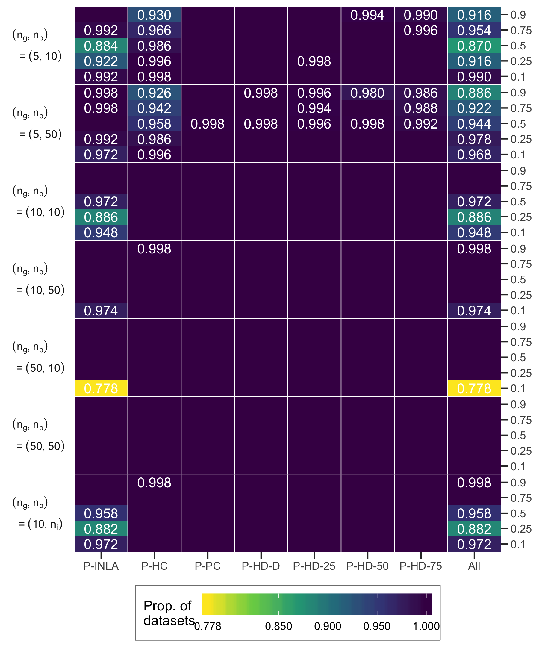
Figure S3.1: The proportion of datasets for each scenario and prior leading to at most 0.1% divergent transitions during the inference in the random intercept model simulation study. We say that the stability is 1.0 if all datasets for a given prior and scenario lead to no more than 0.1% divergent transitions. No number means that the stability is 1.0. The rightmost column, denoted “All”, shows how many datasets must be removed from the study so all priors lead to at most 0.1% divergent transitions for the remaining datasets.

From Figure S3.1 we see that P-INLA is less stable than the other priors, except for datasets with five groups where also P-HC leads to inference with too many divergent transitions. If a dataset leads to more than 0.1% divergent transitions for a given prior, we remove the dataset from the study for this prior. For the scenarios with $n_{\mathrm{g}}=5$, P-INLA and P-HC are more affected by divergent transitions than the other priors. In this case we remove the dataset from the study for all priors. This means that the results for P-INLA is based on fewer simulations than the other priors for $n_{\mathrm{g}}=10$ or $50$.

Figure S3.2: The posterior distribution of the logarithm of the group variance $\sigma_{\alpha}^{2}$ when using Jeffreys’ prior on the residual variance and $\text{InvGamma}(1,5\times 10^{-5})$ on the group variance (P-INLA). The prior on the group variance is included in the plot. We have $n_{\mathrm{g}}=10$ and $n_{i}=10\ \forall i$.

Figure S3.2 shows the posterior distribution of the logarithm of the group variance ($\log(\sigma_{\alpha}^{2})$) when the priors of $\sigma_{\mathrm{R}}^{2}$ and $\sigma_{\alpha}^{2}$ are Jeffreys’ and $\text{InvGamma}(1,5\times 10^{-5})$ (i.e. the INLA default prior), respectively. This is the true posterior, calculated using numerical integration, with a dataset where the maximum likelihood (ML) estimates of the group and residual variances are exactly equal to $\omega$ and $1-\omega$, respectively. We vary the value of $\omega$, and have 10 groups with 10 persons in each. When the true $\omega=0.1$, and most of the variance in the model is residual variance, the posterior is highly influenced by the prior and we have close to no mass at the ML estimate (which is 0.1). When $\omega=0.25$, the posterior is bimodal, and when $\omega=0.5$ almost all the mass is at the ML estimate. This explains the bad results from P-INLA for datasets with true $\omega\leq 0.5$.

Figures S3.3-S3.7 show all the bias and coverage results from the random intercept model simulation study. Note that the coverage of $\omega$ is only shown for values larger than 65%. The order of the priors is the same in the legend and for each scenario in all plots, so P-INLA is the leftmost, so comes P-HC and so on. For a given number of groups and group size, the magnitude of the bias for $\log(V)$ increases and for $\text{logit}(\omega)$ decreases when the true value of $\omega$ increases. This is expected as a larger value of $\omega$ means that the group variance is larger relative to the residual variance and the dataset provides more information about the $\omega$ than would be the case when group variance is small relative to residual variance. On the other hand, a larger $\omega$ means the group variance dominates the total variance $V$ more and there is less information about the group effect, which only has 5, 10 or 50 replicates, than the residual effect, which has 10 or 50 replicates for each group. This means less information about the $V$.

In the following we list the main results from each figure. It is clear from Figure S3.3 that the choice of $\omega_{\mathrm{m}}$ does not have a large impact on the results. For an HD prior with a Dirichlet prior on the weight $\omega$ (P-HD-D), the results are similar for the scenario with equal group and residual variance (true $\omega=0.5$), and worse for the other scenarios. This is true for all dataset sizes. Figure S3.4 shows that also for varying group sizes the HD prior with a PC prior on $\omega$ behaves as well as or better than the other priors in terms of bias and coverage, and again the value of $\omega_{\mathrm{m}}$ does not influence the results noticeably. Figure S3.5 shows that larger groups improves the results in terms of low bias and accurate coverage, especially for P-INLA, but not as much as larger number of groups improves the results. In Figures S3.6 and S3.7 we include results for fewer groups, $n_{\mathrm{g}}=5$, and 10 and 50 persons in each group, respectively. It is difficult to estimate the group variance with a low number of groups, and the results show that P-INLA is performing badly in terms of both bias and coverage for $V$ and $\omega$. For a given scenario with the HD prior, the bias and the coverage both increases for increasing values of $\omega_{\mathrm{m}}$. P-HC leads to the least stable inference for $n_{\mathrm{g}}=5$, and the other five priors give about equally stable inference. Note that for a given scenario we have removed the same datasets from the results for all priors, and the results may be slightly biased because of this.

S3.4 Simulation study for small group sizes

We explore the properties of the HD prior when applied to problems with small datasets with only few observations in each group. Here the amount of information about the parameters is low and the risk of overfitting is high. We define overfitting as overestimating the value of $\omega$, and thus estimating spurious signals in the group effect; and define underfitting as underestimating the value of $\omega$. Specifically, we use a small simulation study with two observations per group, and group size $n_{\mathrm{g}}\in\{10,50,100\}$. We include an additional prior denoted P-HD-10 not included in the main article, which is the HD prior with PC prior on weight with median $\omega_{\mathrm{m}}=0.1$. P-HD-10 is added to explore the option of higher shrinkage in small data settings. The remaining HD priors are introduced in the main article.

From Figure S3.8 one can see that the inference for total variance $V$ is stable in terms of bias and coverage. This indicates that the Jefferey’s prior on $V$ works well also in low information settings. From Figure S3.9, one can see that the inference for the weight $\omega$ depends on the chosen prior. Using the recommended P-HD-25, we are slightly overfitting for the scenario where the true weight is $0.1$, and we are slightly underfitting in the other scenarios. Using stronger shrinkage through P-HD-10 avoids overfitting for true weight equal to $0.1$, but results in a stronger bias for higher values of the true weight, and the resulting coverage varies from 100% to 0% in the scenarios. P-HD-50, P-HD-75 and P-HD-D result in overfitting also for true weight equal to $0.25$ for $n_{g}=10$. The results indicate that the recommended prior P-HD-25 is also appropriate for small group sizes. None of the priors displayed lead to inference with more than 0.1% divergent transitions.

Figure S3.3: The true value of $\omega$ is on the x-axis in all graphs, the two upper rows contain the posterior diagnostics for the log total variance, and the two lower rows for logit weight. Bias in the left column, coverage in the right. The number of groups is indicated at the beginning of each row, either 10 or 50, and the group size $n_{i}=10\ \forall i$. The order of the priors is the same in the legend and for each scenario. The coverage for P-INLA is sometimes below the 65% and not shown in the figure.

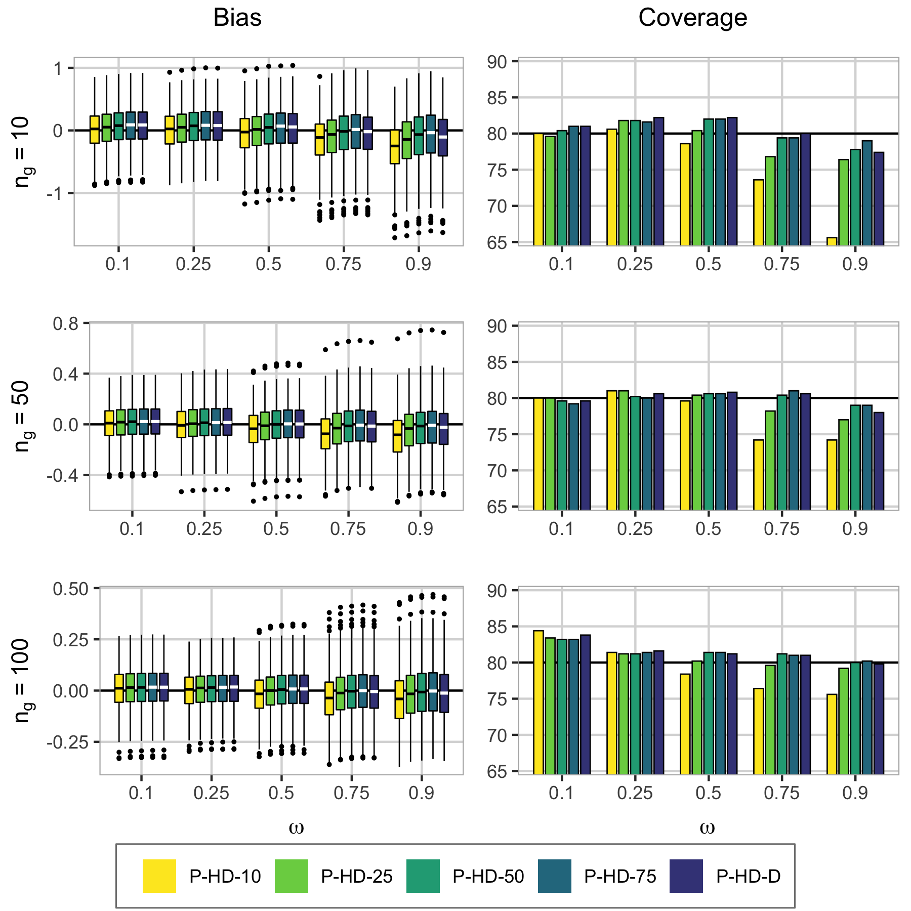
Figure S3.4: The true value of $\omega$ is on the x-axis in all graphs, the upper row contains the posterior diagnostics for the log total variance, and the lower row for logit weight. Bias in the left column, coverage in the right. The number of groups is 10 and the group size $n_{i}$ varies. The order of the priors is the same in the legend and for each scenario. The coverage for P-INLA is sometimes below the 65% and not shown in the figure.

Figure S3.5: The true value of $\omega$ is on the x-axis in all graphs, the two upper rows contain the posterior diagnostics for the log total variance, and the two lower rows for logit weight. Bias in the left column, coverage in the right. The number of groups is indicated at the beginning of each row, either 10 or 50, and the group size $n_{i}=50\ \forall i$. The order of the priors is the same in the legend and for each scenario. The coverage for P-INLA is sometimes below the 65% and not shown in the figure.

Figure S3.6: The true value of $\omega$ is on the x-axis in all graphs, the upper row contains the posterior diagnostics for the log total variance, and the lower row for logit weight. Bias in the left column, coverage in the right. The number of groups $n_{\mathrm{g}}=5$, and the group size $n_{i}=10\ \forall i$. The order of the priors is the same in the legend and for each scenario. The coverage for P-INLA is sometimes below the 65% and not shown in the figure.

Figure S3.7: The true value of $\omega$ is on the x-axis in all graphs, the upper row contains the posterior diagnostics for the log total variance, and the lower row for logit weight. Bias in the left column, coverage in the right. The number of groups $n_{\mathrm{g}}=5$, and the group size $n_{i}=50\ \forall i$. The order of the priors is the same in the legend and for each scenario. The coverage for P-INLA is sometimes below the 65% and not shown in the figure.

Figure S3.8: Results for $\log(V)$. The true value of $\omega$ is on the x-axis in all graphs, bias is shown in the left column, coverage in the right. The number of groups is indicated at the beginning of each row, and there are two persons in each group. The order of the priors is the same in the legend and for each scenario.

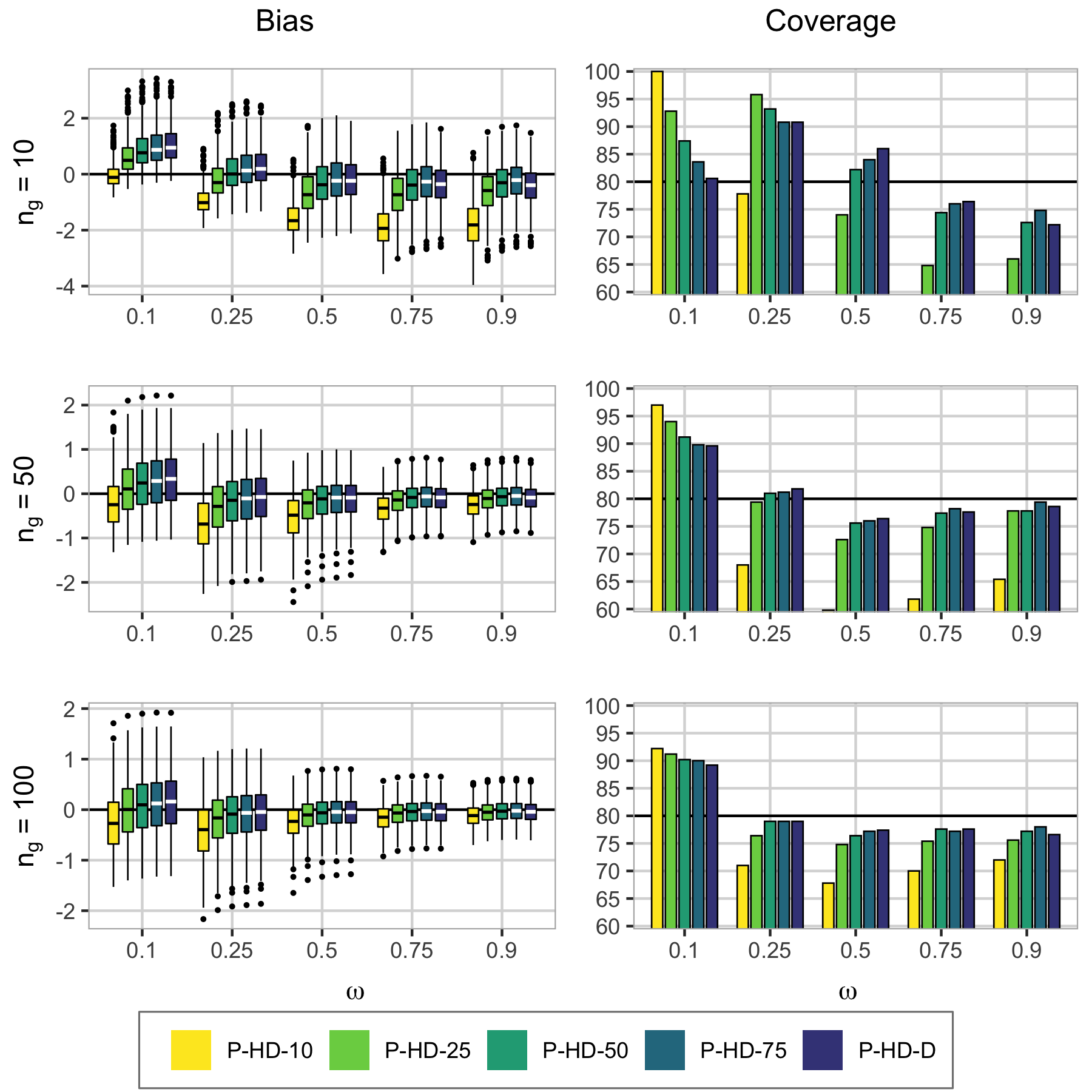
Figure S3.9: Results for $\text{logit}(\omega)$. The true value of $\omega$ is on the x-axis in all graphs, bias is shown in the left column, coverage in the right. The number of groups is indicated at the beginning of each row, and there are two persons in each group. The order of the priors is the same in the legend and for each scenario. The coverage for P-HD-10 is sometimes below the 65% and not shown in the figure.

S4 Gaussian responses: Latin square

We include additional background and all results from the latin square simulation study from Section 5.2 in the main article.

S4.1 Additional background

The reasoning behind the tree structure for the prior in the latin square simulation study displayed in Figure 1(a) is as follows: At the first level (top level) the prior shrinks the latent part of the model, at the second level the total latent variance is distributed with equal preference to the row effect, the column effect and the treatment effect, and at the third level the treatment effect is shrunk towards the unstructured effect. We select an HD prior using the model structure in Figure 1(a). We also implement the triple split as explained in Section S2. The original order chosen in the main article is denoted Order1 (1(b)), and the permuted orders Order2 (1(c)) and Order3 (1(d)). The total variance of the latent model is split into $\omega^{(1)}$, $\omega^{(2)}$ and $\omega^{(3)}$, which are the proportions of the latent variance going to the row effect, column effect and the treatment effect, respectively. Figure S4.3 shows the difference in marginal priors for $\omega^{(1)}$, $\omega^{(2)}$ and $\omega^{(3)}$ for Order1 and Order2, on weight scale and on logit weight scale. Figure S4.4 shows the difference in the same marginal priors for Order1 and a Dirichlet prior on the triple split, where the latter is the default choice in the HD prior framework.

(a) Multi-split structure

(b) Dual-split structure, original order (Order1)

(c) Dual-split structure, permuted order (Order2)

(d) Dual-split structure, permuted order (Order3)

Figure S4.1: Two of the possible orderings for turning the triple split into a dual split. 1(a)) The multi-split structure of the HD prior, 1(b)) the original order used in simulation study in paper (Order1), 1(c)) one permuted order (Order2), and 1(d)) the other permuted order (Order2)

The true treatment effect $\bm{x}=(x_{1},\ldots,x_{9})$ we use in the latin square simulation study is given by $x_{i}=C\left((i-5)^{2}-20/3\right)$, $i=1,\ldots,9$ where $C=0$ for scenario S1, $C=0.05$ for scenario S2, and $C=0.2$ for scenario S3. These corresponds to signal to noise ratios (SNRs) of $0\%$, $48\%$ and $94\%$ for S1, S2 and S3, respectively, as computed by $\text{SNR}=S_{xx}/(S_{xx}+\sigma_{\mathrm{t}}^{2})$, where $S_{xx}=\sum_{i=1}^{9}(x_{i}-\bar{x})^{2}$. Figure S4.2 shows the true treatment effect for the three scenarios.

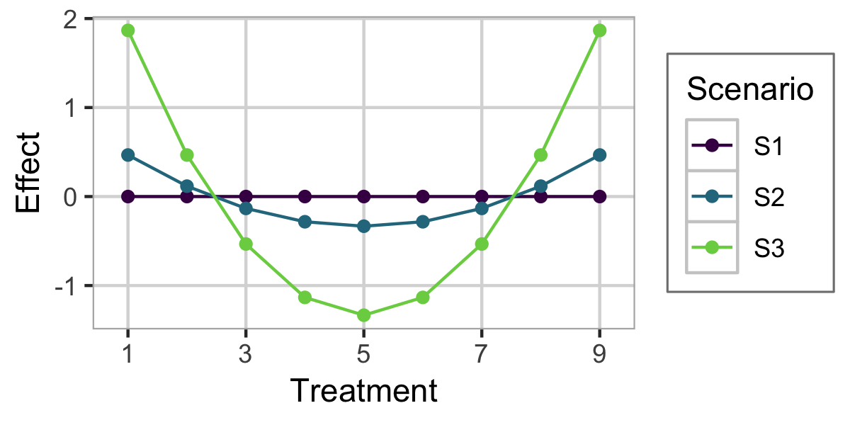
Figure S4.2: The true treatment effect for the simulated datasets in the latin square simulation study.

In the latin square experiment we use the following settings in the R-function stan: a burn-in of length 25 000, a total sample number (including burn-in) of 125 000, one chain which we thin to every fifth sample, we initialize all parameters to zero, and use adapt_delta equal to 0.95. We use default values for the rest of the settings. For the leave-one-out log predictive score (LOO-LPS), we use 1000 simulations for warm-up and 2000 samples in total, which yields a low estimated variance of the LOO-LPS. The simulation study ran on a computer cluster and takes no more than a couple of days, depending on the activity on the cluster.

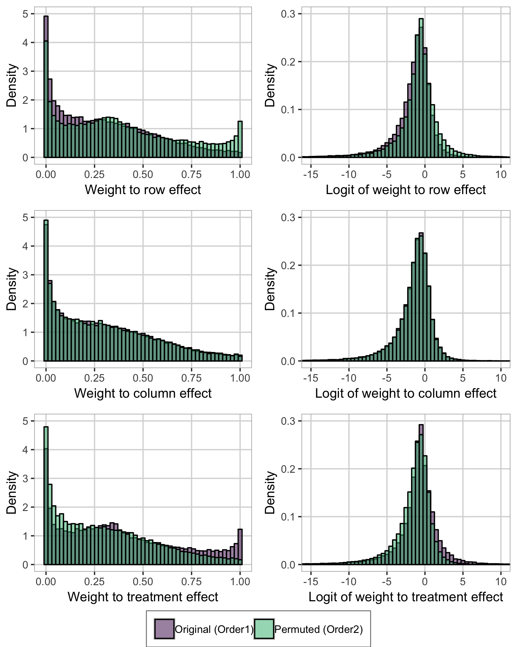
Figure S4.3: Comparison of priors on distribution of total latent variance to row effect, column effect and treatement effect for the original order Order1 and the permuted order Order2. The distributions of the weights to the left, and of the logit weights on the right.

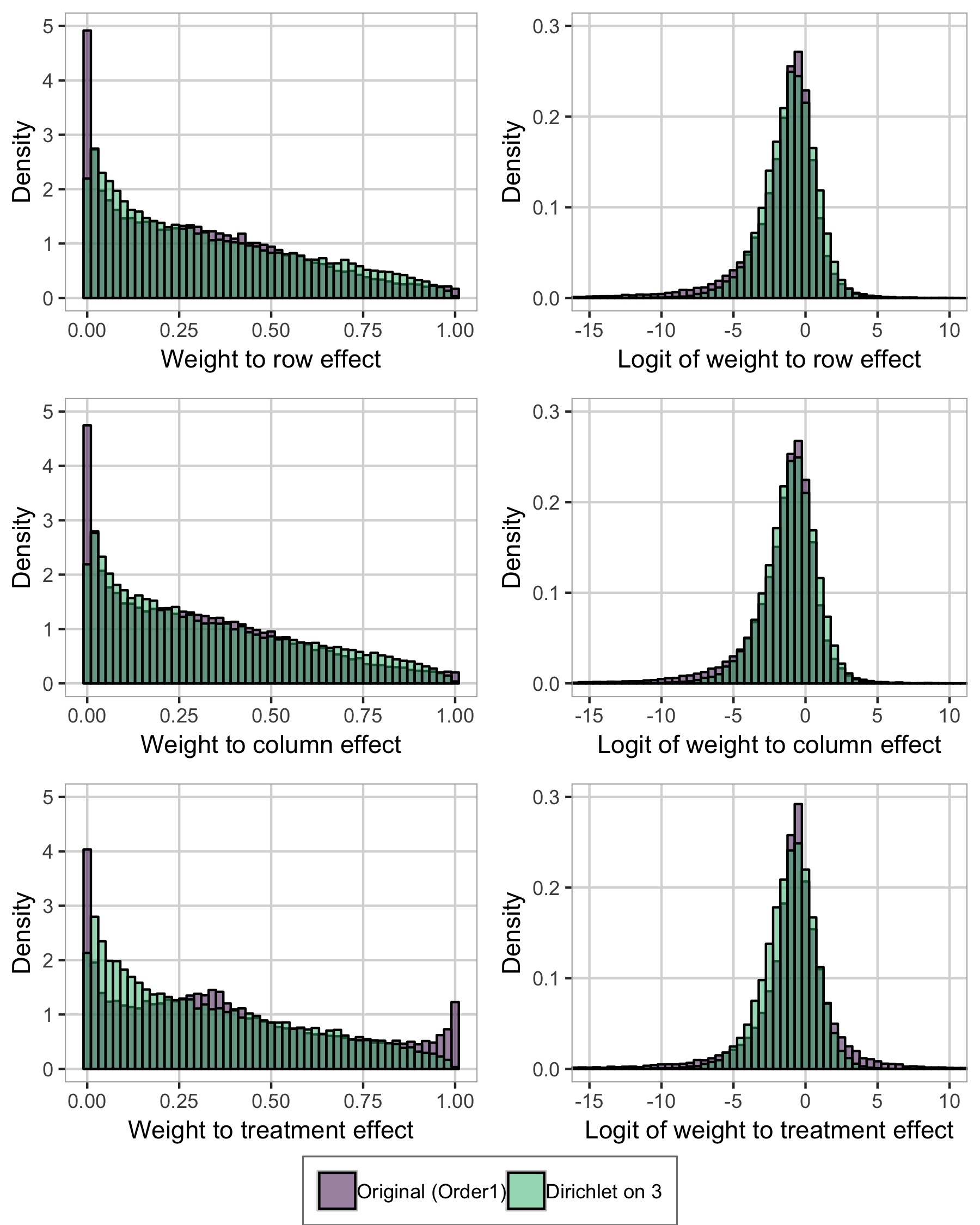
Figure S4.4: Comparison of priors on distribution of total latent variance to row effect, column effect and treatement effect for the original order Order1 and a Dirichlet prior on the triple split. The distributions of the weights to the left, and of the logit weights on the right.

S4.2 Results

We have investigated the properties of the HD prior when the principles of the framework are tweaked. What we investigate is varying values of the median $\omega_{\mathrm{m}}$ of the prior on the weight indicating the proportion of treatment variance going to the structured effect, varying distributions on the distance in the original PC prior framework, varying the value of $\lambda$ for the multi-split, varying the type and ordering of the multi-split (see Figure S4.1), and we also study a joint prior where we use a Dirichlet prior on all effects except the residuals, and on all five effects. We compare the HD prior to the following default priors, where all have Jeffreys’ prior on the residual variance and the following priors on the remaining variances or standard deviations: $\text{InvGamma}(1,5\times 10^{-5})$ (P-INLA), $\text{Half-Cauchy}(25)$ (P-HC), and $\text{PC}_{\mathrm{SD}}(3,0.05)$ (P-PC).

For each scenario, we have removed the datasets that lead to more than 0.1% divergent transitions for at least one of the priors, so all the results for a given scenario are based on the same datasets for all priors. We use the proportion of datasets leading to at most 0.1% divergent transitions during the inference as a measure of stability, for each prior and scenario. Figure S4.5 displays these proportions for the latin square simulation study, and we see that it is not a big difference between P-INLA, P-HC, P-PC, and P-HD-25. However, when we lower the value of the shape parameter in the distribution we use on the distance (tweaking the third principle of the PC prior), the number of divergent transitions occurring during the inference increases, which indicates a more difficult posterior to draw samples from. When we change the values of $\omega_{\mathrm{m}}$, $\lambda$, or the way we implement the triple split (see Figure S4.1) the stability of the inference does not suffer.

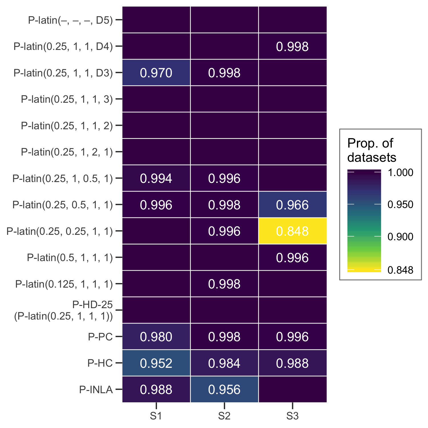
Figure S4.5: The proportion of datasets for each scenario and prior leading to at most 0.1% divergent transitions during the inference in the latin square experiment simulation study. We say that the stability is 1.0 if all datasets for a given prior and scenario lead to no more than 0.1% divergent transitions. No number means that the stability is 1.0. The bottom four priors are the main focus of the study, the top three are the Dirichlet priors, while the middle eight are the HD prior with varying values of $\omega_{\mathrm{m}}$, amount of shrinkage, varying values of $\lambda$, and varying ordering of the implementation of the triple split. The notation for the HD prior is P-latin($\omega_{\mathrm{m}}$, shape parameter, $\lambda$, order number/type).

Figures S4.6-S4.11 show all results from the latin square simulation study. The box-plots include the median, the first and third quartile, 1.5 times the inter-quartile range (distance between first and third quartile), and outliers, if any. The six graphs all show the continuous rank probability score (CRPS) of the structured treatment effect $\bm{\gamma}^{(1)}$ and the leave-one-out log predictive score (LOO-LPS). In each plot, we have removed the datasets leading to too many (i.e., more than 0.1%) divergent transitions in the inference for at least one of the three priors displayed. The order of the priors is the same in the legend and for each scenario in all plots, so P-INLA is the leftmost, so comes P-HC and so on.

Figure S4.6 shows the results that are also displayed in the main paper: P-INLA gives a lower LOO-LPS, i.e. a poorer model fit, than the other priors. The CRPS is lowest for the HD prior with either triple split implementation for scenarios S2 and S3. Figure S4.7 shows results for varying values of the median $\omega_{\mathrm{m}}$ for the prior for selecting between $\bm{\gamma}^{(1)}$ and $\bm{\gamma}^{(2)}$ has little effect on the results, and we see that a lower value of the median is slightly better when the true treatment effect is weak, and a higher value is slightly better when the true treatment effect is strong. The difference is however small. Figure S4.8 shows the results when we change the distribution we use on the distance between $\bm{\gamma}^{(1)}$ and $\bm{\gamma}^{(2)}$. Changing the exponential prior on the distance between $\bm{\gamma}^{(1)}$ and $\bm{\gamma}^{(2)}$ to a gamma prior with shape parameter $0.5$ or $0.25$, which has a stronger peak at 0, improves results for S1 (see Figure S4.8), but induces more instability in the inference (Figure S4.5). The results are also stable to changes in the hyperparameter for the two dual-splits (Figure S4.9) and changes in the way that the triple-split is implemented; either decomposed into dual-splits in different ways (Figure S4.10) or using a Dirichlet distribution (Figure S4.11).

We have compared the HD prior with a Dirichlet prior on the triple split (P-HD-D3) to HD priors with a Dirichlet prior on a quadruple split between $\bm{\alpha}$, $\bm{\beta}$, $\bm{\gamma}^{(1)}$ and $\bm{\gamma}^{(2)}$ (P-HD-D4) and between all five effects (P-HD-D5). The two latter perform worse than P-HD-D3 when the treatment effect has no structured contribution, scenario S1, in terms of CRPS (Figure S4.11). Using P-HD-D4 and P-HD-D5 we lose the shrinkage properties between the unstructured and structured treatment effect, so we expect them to perform worse for S1. For S2 and S3 they perform slightly better. The LOO-LPS is not affected noticeably by the implementation of the triple split.

Figure S4.6: Results from the latin square simulation study.

Figure S4.7: Results from the latin square simulation study when varying the position of the median $\omega_{\mathrm{m}}$ in the PC prior on the distance between $\bm{\gamma}^{(1)}$ and $\bm{\gamma}^{(2)}$. $\omega_{\mathrm{m}}=0.25$ gives P-HD-25.

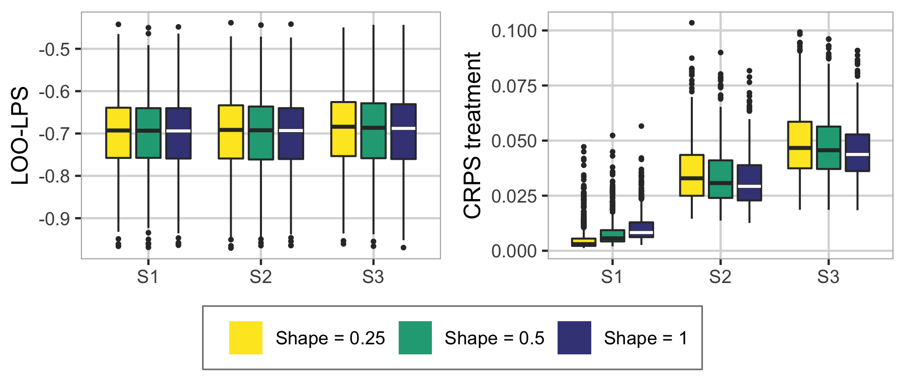
Figure S4.8: Results from the latin square simulation study when varying the shape parameter in the distribution on the distance in the PC prior for the split between unstructured and structured treatment effect. Shape parameter 1 gives the exponential distribution, which gives P-HD-25.

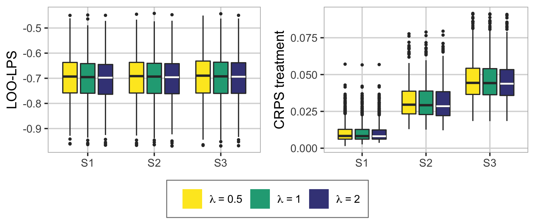
Figure S4.9: Results from the latin square simulation study when varying the value of $\lambda$ in the PC prior for the multi split. $\lambda=1$ gives P-HD-25.

Figure S4.10: Results from the latin square simulation study when varying order of the implementation of the triple split in the PC prior. Order1 gives P-HD-25.

Figure S4.11: Results from the latin square simulation study for the Dirichlet prior. P-HD-D3 has a Dirichlet prior on the split between the row, column and treatment effects, P-HD-D4 has a Dirichlet prior between all effects except the residuals, and P-HD-D5 has a Dirichlet prior on all five random effects (including the residuals). The other weights has PC priors as in P-HD-25.

S4.3 Example

We provide a script for R that can be used to simulate data and fit the latin square model. The script is available as part of the Supplementary Materials. This script can be used to look at differences between the priors and the resulting posteriors.

The following priors from the simulation study can be chosen:

1. INLA default (P-INLA)

2. Half-Cauchy (P-HC)

3. Component-wise PC priors (P-PC)

4. HD prior with PC priors on all splits (for example, P-HD-25). Here you can choose to change

   • the median $\omega_{\mathrm{m}}$ for the proportion of treatment variance going to the structured effect [0.25 is default],

   • the shape parameter for the gamma distribution on the distance between the unstructured and structured treatment effect [1 is default],

   • A scaling factor for the value of $\lambda$ used in the multi-splits [1 is default],

   • the ordering of the triple split [1 is default, 2 and 3 are the other orderings].

5. HD prior with a combination of PC and Dirichlet priors (for example, P-HD-D3). Here you can choose to change

   • the number of effects involved in the Dirichlet prior in the HD prior [3 is default, 4 and 5 are the other options].

After the prior has been chosen, the scenario can be selected: scenario S1 (no treatment effect), S2 (medium treatment effect) or S3 (strong treatment effect). See Section S4.1 for details. A dataset of the same size as the ones in the simulation study is simulated, and the dataset can be reproduced using a seed value.

Rstan is used for the inference, and you can choose between the following number of samples: "low" (250 (warmup) + 1000, only for testing, this will not give enough samples), "medium" (2500 (warmup) + 10000) or "high" (25000 (warmup) + 100000, this is used in the simulation study in the paper).

The sampler can be run without the likelihood to sample from the prior. A plot of the prior on total weight (the amount of the total variance) for each of the five effects in the model is available. The prior on total variance and the separate variances for the effects are not shown as they do not have proper priors under the scale-invariant HD priors or Jeffreys’ prior on the residual variance.

For the posterior, the following scores and plots are provided:

• The number of divergent transitions that occurred during the inference (see e.g. Section S3.1).

• The posterior total weights for the five model effects and the posterior total variance.

• The posterior standard deviations for the five model effects.

• The posterior mean of the structured treatment effect, with standard deviations, compared to the true effect.

• The average CRPS of the structured treatment effect, see Section 5.2 in the main article for details.

• The LOO-LPS (see Section 5.2 in the main article for details), with corresponding variance of the estimate, and the number of the 81 inferences with more than 1% divergent transitions.

S5 Binomial responses

We include additional background and results from the Kenyan neonatal mortality simulation study and real application presented in Section 6 in the main article.

S5.1 Additional background

The DHS survey from 2014 is stratified by county and urban/rural and has two levels of clustering. Since the counties Nairobi and Mombasa are fully urban, there are in total 92 strata. The households were selected within each stratum through a two-stage clustered sampling design. Kenya was divided into 96251 enumeration areas (EAs) based on the 2009 national census, and the first stage of the sampling design consists of sampling clusters from the list of EAs in the stratum and the second stage consists of sampling households within the selected clusters. Within the selected households all women aged 15–49 who spent the last night in the household are interviewed.

In Section 6.2 in the main paper, we simulate from a model consisting of spatially structured and unstructured random effects and an i.i.d. effect of cluster. Further, preliminary investigations showed that the design with 47 counties provides little information about how the variance should be distributed between the structured and the unstructured spatial effect. Therefore, we use the 290 constituencies of Kenya with 6 clusters per constituency to replicate the size of the survey, but provide a spatial design where the data is more informative about the relative sizes of the unstructured and structured spatial effects. In Section 6.3 in the main paper we analyse the original data on the county-level and include a random effect of household. The key focus of the application is to display how to use and select the new prior, and how the interpretability and transparency of the prior is helpful for assessing and criticising the results.

S5.2 Simulation study

We use the following input values to the function stan for the simulation study with neonatal mortality in Kenya: 25 000 samples for burn-in, in total 75 000 samples, one chain thinned to every fifth sample, all parameters initialized to zero, adapt_delta equal to 0.95, and default settings for all other input values. The simulation study ran on a computer cluster and takes less than a week, depending on the activity on the cluster.

We include additional results from the Kenya neonatal mortality simulation study. Figure S5.1 shows the proportion of datasets leading to no more than 0.1% divergent transitions during the inference. P-INLA is the only prior which leads to a large number of datasets giving divergent transitions, and mainly in scenario S3, the other three priors give stable inference for all scenarios. Figure S5.2 shows the bias and coverage of $\mu$, the the bias of $\omega^{(1)}$ and $\omega^{(2)}$ and the CRPS of $\bm{u}$, for the five priors we have used in the simulation study. It is only for scenario S3, when the Dirichlet prior is closest to the truth, that P-HD-D is performing better than P-HD-25, in the other scenarios it is doing worse.

Figure S5.2 shows that P-INLA gives way too low coverage for $\mu$, while the other priors leads to a better and similar coverage. For scenarios S2-S5 the true value of the weight is 0.2, P-INLA is for most datasets estimating $\omega^{(1)}$ to be 0, giving a bias of -0.2. The other four priors are all slightly underestimating the weight in S2-S5. P-HD-D is as good as (only scenario S3) or worse than P-HD-25. In scenario S1, the true weight is equal to 1 while the base model is 0, and all priors are underestimating the weight. P-INLA is doing worst with a bias around -0.75 for most datasets, while P-HD-25 is doing a bit better with a bias of around -0.5, and P-HC and P-PC are also underestimating the weight. This may be an indication that we get the prior back, and that the likelihood does not contribute much in the inference.

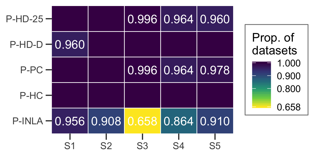
Figure S5.1: The proportion of datasets for each scenario and prior leading to at most 0.1% divergent transitions during the inference in the neonatal mortality in Kenya simulation study. We say that the stability is 1.0 if all datasets for a given prior and scenario lead to no more than 0.1% divergent transitions. No number means that the stability is 1.0.

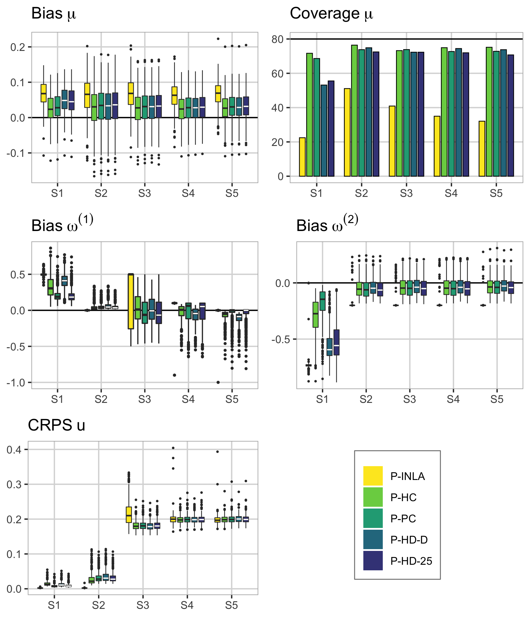
Figure S5.2: Upper left: bias of the intercept $\mu$, upper right: the coverage of $\mu$, mid left: the bias of $\omega^{(1)}$, mid right: the bias of $\omega^{(2)}$, and lower left: CRPS of $\bm{u}$. Scenario is indicated at the x-axes. The order of the priors is the same in the legend and for each scenario, so P-INLA is the leftmost, then comes P-HC and so on. The biases are calculated using the estimated median minus the true value, and the coverage is found by counting the number of times the true value lies in the 80% credible interval.

S5.3 Application

The prior and posterior of the total standard deviation from the Kenya neonatal mortality dataset analysis can be seen in Figure S5.3.

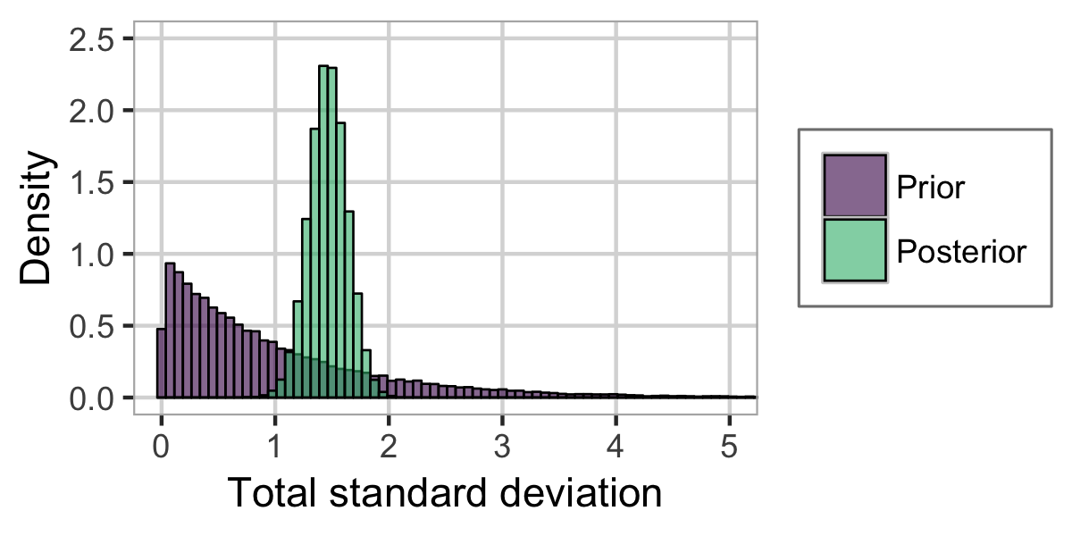
Figure S5.3: The prior and posterior of the total standard deviation $\sigma_{\mathrm{T}}$ from the analysis of the neonatal mortality in Kenya dataset.

The prior and posterior distributions of the total weight of the unstructured random effects $v$ (unstructured county effect), $\nu$ (unstructured cluster effect) and $\varepsilon$ (unstructured household effect) can be seen in Figure S5.4. The total weight is $\omega^{(1)}$ for $\varepsilon$, $\omega^{(2)}(1-\omega^{(1)})$ for $\nu$, and $(1-\omega^{(3)})(1-\omega^{(2)})(1-\omega^{(1)})$ for $v$. The medians of these three are $0.955$, $0.014$ and $0.011$, respectively. It is clear that the household effect $\varepsilon$ explains most of the variance, the cluster effect $\nu$ explains some, and the unstructured county effect $v$ explains the least of the three.

Figure S5.4: The priors and posteriors of the proportion of the total latent variance assigned to the household effect, the cluster effect, and the unstructured spatial effect.

Figure S5.5 shows how far a value of $0$ is from the posterior median of $\bm{u}$ expressed by the posterior tail probability of getting 0 or further away from the median. We see that for many counties the posterior median of $u$ is close to 0 as expressed by the value 0.5 in the figure, and 0 is at the most barely outside the interquartile range as expressed by a value of 0.25.

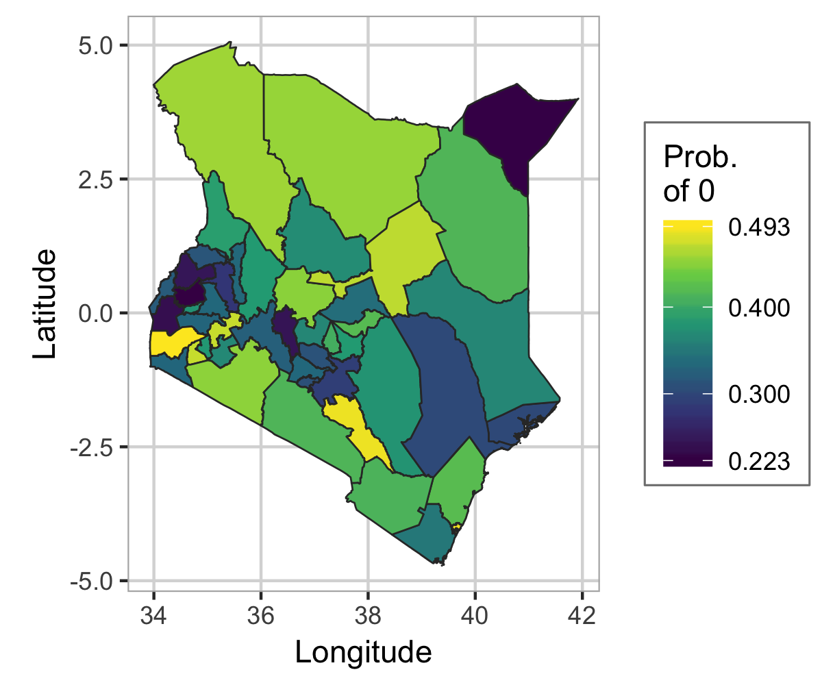
Figure S5.5: The significance of the spatial effect $\bm{u}$ visualized through the tail probabilities $\text{Prob}(u_{i}>0)$ for the counties where the median of $\bm{u}$ is smaller than 0, and $\text{Prob}(u_{i}<0)$ for the counties where the median of $\bm{u}$ is larger than 0.

References

-
Bakka et al. (2018)
Bakka, H., H. Rue, G.-A. Fuglstad, A. Riebler, D. Bolin, J. Illian,
E. Krainski, D. Simpson, and F. Lindgren
2018. Spatial modeling with r-inla: A review. Wiley Interdisciplinary Reviews: Computational Statistics, 10(6):e1443. -
Balakrishnan and
Nevzorov (2003)
Balakrishnan, N. and V. B. Nevzorov
2003. A primer on statistical distributions. Hoboken, NJ: John Wiley & Sons. -
Banerjee et al. (2014)
Banerjee, S., B. P. Carlin, and A. E. Gelfand
2014. Hierarchical Modeling and Analysis for Spatial Data. Boca Raton, FL: Chapman and Hall/CRC. -
Besag et al. (1991)
Besag, J., J. York, and A. Mollié
1991. Bayesian image restoration, with two applications in spatial statistics. Annals of the Institute of Statistical Mathematics, 43(1):1–20. -
Bhattacharya
et al. (2015)
Bhattacharya, A., D. Pati, N. S. Pillai, and D. B.
Dunson
2015. Dirichlet–laplace priors for optimal shrinkage. Journal of the American Statistical Association, 110(512):1479–1490. -
Blangiardo and Cameletti (2015)
Blangiardo, M. and M. Cameletti
2015. Spatial and spatio-temporal Bayesian models with R-INLA. West Sussex, United Kingdom: John Wiley & Sons. -
Carpenter et al. (2017)
Carpenter, B., A. Gelman, M. D. Hoffman, D. Lee, B. Goodrich, M. Betancourt,
M. Brubaker, J. Guo, P. Li, and A. Riddell
2017. Stan: A probabilistic programming language. Journal of Statistical Software, 76(1). -
Cicchetti (1994)
Cicchetti, D. V.
1994. Guidelines, criteria, and rules of thumb for evaluating normed and standardized assessment instruments in psychology. Psychological assessment, 6(4):284. -
Fahrmeir and Lang (2001)
Fahrmeir, L. and S. Lang
2001. Bayesian inference for generalized additive mixed models based on markov random field priors. Journal of the Royal Statistical Society: Series C, 50(2):201–220. -
Fuglstad et al. (2019)
Fuglstad, G.-A., D. Simpson, F. Lindgren, and
H. Rue
2019. Constructing priors that penalize the complexity of gaussian random fields. Journal of the American Statistical Association, 114(525):445–452. -
Gelman (2006)
Gelman, A.
2006. Prior distributions for variance parameters in hierarchical models. Bayesian Analysis, 1(3):515–534. -
Gelman et al. (2013)
Gelman, A., J. B. Carlin, H. S. Stern, D. B. Dunson, A. Vehtari, and D. B.
Rubin
2013. Bayesian Data Analysis. Boca Raton, FL: Chapman and Hall/CRC. -
Gelman and Hill (2007)
Gelman, A. and J. Hill
2007. Data Analysis Using Regression and Multilevel/Hierarchical Models, volume 1. New York, New York: Cambridge University Press. -
Gelman et al. (2008)
Gelman, A., A. Jakulin, M. G. Pittau, Y.-S. Su,
et al.
2008. A weakly informative default prior distribution for logistic and other regression models. The Annals of Applied Statistics, 2(4):1360–1383. -
Gelman et al. (2017a)
Gelman, A., D. Simpson, and M. Betancourt
2017a. The prior can often only be understood in the context of the likelihood. Entropy, 19(10):555. -
Gelman et al. (2017b)
Gelman, A., D. Simpson, and M. Betancourt
2017b. The prior can often only be understood in the context of the likelihood. Entropy, 19(10):555. -
General Assembly of the United
Nations (2015)
General Assembly of the United Nations
2015. Resolution adopted by the General Assembly on 25 September 2015. A/RES/70/1. -
Gneiting and Raftery (2007)
Gneiting, T. and A. E. Raftery
2007. Strictly proper scoring rules, prediction, and estimation. Journal of the American Statistical Association, 102(477):359–378. -
Golding et al. (2017)
Golding, N., R. Burstein, J. Longbottom, A. J. Browne, N. Fullman,
A. Osgood-Zimmerman, L. Earl, S. Bhatt, E. Cameron, D. C. Casey,
et al.
2017. Mapping under-5 and neonatal mortality in africa, 2000–15: a baseline analysis for the sustainable development goals. The Lancet, 390(10108):2171–2182. -
Guo et al. (2017)
Guo, J., A. Riebler, and H. Rue
2017. Bayesian bivariate meta-analysis of diagnostic test studies with interpretable priors. Statistics in Medicine, 36(19):3039–3058. -
Hinkelmann and Kempthorne (1994)
Hinkelmann, K. and O. Kempthorne
1994. Design and Analysis of Experiments, Volume 1: Introduction to Experimental Design. John Wiley & Sons. -
Holand et al. (2013)
Holand, A. M., I. Steinsland, S. Martino, and
H. Jensen
2013. Animal models and integrated nested Laplace approximations. G3: Genes, Genomes, Genetics, Pp. g3–113. -
Jordan et al. (2017)
Jordan, A., F. Krüger, and S. Lerch
2017. Evaluating probabilistic forecasts with the r package scoringrules. arXiv preprint arXiv:1709.04743. -
Kenya National Bureau of Statistics
et al. (2015)
Kenya National Bureau of Statistics, Ministry of Health/Kenya, National
AIDS Control Council/Kenya, Kenya Medical Research Institute, and
National Council for Population and
Development/Kenya
2015. Kenya Demographic and Health Survey 2014. Rockville, MD, USA: [publisher unknown]. -
Krainski et al. (2018)
Krainski, E. T., V. Gómez-Rubio, H. Bakka, A. Lenzi, D. Castro-Camilio,
D. Simpson, F. Lindgren, and H. Rue
2018. Advanced Spatial Modeling with Stochastic Partial Differential Equations using R and INLA. Boca Raton, FL: CRC press. Github version www.r-inla.org/spde-book. -
Lambert et al. (2005)
Lambert, P. C., A. J. Sutton, P. R. Burton, K. R. Abrams, and D. R.
Jones
2005. How vague is vague? a simulation study of the impact of the use of vague prior distributions in MCMC using WinBUGS. Statistics in Medicine, 24(15):2401–2428. -
Li et al. (2019)
Li, Z., Y. Hsiao, J. Godwin, B. D. Martin, J. Wakefield, S. J. Clark,
et al.
2019. Changes in the spatial distribution of the under-five mortality rate: Small-area analysis of 122 dhs surveys in 262 subregions of 35 countries in africa. PloS one, 14(1):e0210645. -
Lindgren and Rue (2015)
Lindgren, F. and H. Rue
2015. Bayesian spatial modelling with r-inla. Journal of Statistical Software, 63(19):1–25. -
Lindgren et al. (2011)
Lindgren, F., H. Rue, and J. Lindström
2011. An explicit link between gaussian fields and gaussian markov random fields: the stochastic partial differential equation approach. Journal of the Royal Statistical Society: Series B (Statistical Methodology), 73(4):423–498. -
Lunn et al. (2009)
Lunn, D., D. Spiegelhalter, A. Thomas, and
N. Best
2009. The bugs project: Evolution, critique and future directions. Statistics in Medicine, 28(25):3049–3067. -
Martinez-Beneito (2013)
Martinez-Beneito, M. A.
2013. A general modelling framework for multivariate disease mapping. Biometrika, 100(3):539–553. -
McGraw and Wong (1996)
McGraw, K. O. and S. P. Wong
1996. Forming inferences about some intraclass correlation coefficients. Psychological methods, 1(1):30. -
Plummer (2017)
Plummer, M.
2017. JAGS version 4.3. 0 user manual [Computer software manual]. Retrieved from sourceforge. net/projects/mcmc-jags/files/Manuals/4.x. -
Polson and Scott (2010)
Polson, N. G. and J. G. Scott
2010. Shrink globally, act locally: Sparse bayesian regularization and prediction. Bayesian statistics, 9:501–538. -
Riebler et al. (2016)
Riebler, A., S. H. Sørbye, D. Simpson, and
H. Rue
2016. An intuitive Bayesian spatial model for disease mapping that accounts for scaling. Statistical Methods in Medical Research, 25(4):1145–1165. -
Rue and Held (2005)
Rue, H. and L. Held
2005. Gaussian Markov random fields: theory and applications. Boca Raton, Florida: CRC press. -
Rue and Held (2010)
Rue, H. and L. Held
2010. Discrete spatial variation. In Handbook of Spatial Statistics, A. E. Gelfand, P. Diggle, P. Guttorp, and M. Fuentes, eds., Handbooks of Modern Statistical Methods, chapter 12, Pp. 171–200. Boca Raton, FL: CRC Press. -
Rue et al. (2009)
Rue, H., S. Martino, and N. Chopin
2009. Approximate Bayesian inference for latent Gaussian models by using integrated nested Laplace approximations. Journal of the Royal Statistical Society: Series B, 71(2):319–392. -
Rue et al. (2017)
Rue, H., A. Riebler, S. H. Sørbye, J. B. Illian, D. P. Simpson, and F. K.
Lindgren
2017. Bayesian computing with inla: A review. Annual Review of Statistics and Its Application, 4(1):395–421. -
Shen et al. (2016)
Shen, K.-K., V. Doré, S. Rose, J. Fripp, K. L. McMahon, G. I. de Zubicaray,
N. G. Martin, P. M. Thompson, M. J. Wright, and
O. Salvado
2016. Heritability and genetic correlation between the cerebral cortex and associated white matter connections. Human brain mapping, 37(6):2331–2347. -