Low-redshift lowest-metallicity star-forming galaxies in the SDSS DR14

We present a sample of low-redshift ($z$ $<$ 0.133) candidates for extremely low-metallicity star-forming galaxies with oxygen abundances 12 + logO/H $<$ 7.4 selected from the Data Release 14 (DR14) of the Sloan Digital Sky Survey (SDSS). Three methods are used to derive their oxygen abundances. Among these methods two are based on strong [O ii]$\lambda$3727$\AA$, [O iii]$\lambda$4959$\AA$, and [O iii]$\lambda$5007$\AA$ emission lines, which we call strong-line and semi-empirical methods. These were applied for all galaxies. We have developed one of these methods, the strong-line method, in this paper. This method is specifically focused on the accurate determination of metallicity in extremely low-metallicity galaxies and may not be used at higher metallicities with 12 + logO/H $\ga$ 7.5. The third, the direct $T_{\rm e}$ method, was applied for galaxies with detected [O iii] $\lambda$4363 emission lines. All three methods give consistent abundances and can be used in combination or separately for selection of lowest-metallicity candidates. However, the strong-line method is preferable for spectra with a poorly detected or undetected [O iii]$\lambda$4363 emission line. In total, our list of selected candidates for extremely low-metallicity galaxies includes 66 objects.

1 Introduction

Nearby dwarf star-forming galaxies (SFG) with extremely low metallicities are often considered as local counterparts of high-redshift galaxies. Their proximity allows us to study them in much greater detail than the high-redshift galaxies and to establish useful constraints on the physical conditions of their low-metallicity interstellar medium (ISM), the origin of chemical elements, and to develop models of stellar evolution. These studies can be used to analyse the physical properties of the primeval galaxies at redshifts $z$ $\sim$ 5 - 10, which are thought to be dwarf systems responsible for the reionization of the Universe (Ouchi et al. 2009; Wise & Chen 2009; Bouwens et al. 2015; Robertson et al. 2013, 2015; Khaire et al. 2016).

However, the number of known nearby lowest-metallicity SFGs with oxygen abundances 12 + logO/H $\la$ 7.35 is very low. Among them are SFGs with 12 + logO/H $\sim$ 7.00. These are J0811$+$4730 with 12 + logO/H = 6.98$\pm$0.02 (Izotov et al. 2018a), A198691 with 12 + logO/H = 7.02$\pm$0.03 (Hirschauer et al. 2016) and SBS 0335$-$052W with 12 + logO/H ranging from 6.86 to 7.22 in different star-forming regions (Izotov et al. 2009). Recently, Annibali et al. (2019) reported the range 6.96 – 7.14 in different H ii regions of DDO 68. Additionally, Pustilnik et. al. (2016) and Kniazev et al. (2018) derived 12 + logO/H $\la$ 7.35 in nearly a dozen of galaxies in the Lynx-Cancer and Eridanus voids.

Large spectroscopic surveys, such as the Sloan Digital Sky Survey (SDSS) containing millions of galaxy spectra in its database, open an opportunity to considerably increase the sample of the extremely low-metallicity SFGs with 12 + logO/H $\la$ 7.35 (e.g. Izotov et al. 2012; Guseva et al. 2017). In particular, the SFG with a record low luminosity-weighted metallicity, J0811$+$4730, was found in the SDSS.

The empirical diagnostic [O iii] $\lambda$5007/H$\beta$ - [N ii] $\lambda$6584/H$\alpha$ diagram (Baldwin et al. 1981) can successfully be used to preselect the candidates to extremely low-metallicity SFGs. On this diagram, they occupy the region with both very low [O iii] $\lambda$5007/H$\beta$ $\leq$ 3 and very low [N ii] $\lambda$6584/H$\alpha$ $\leq$ 0.1, far from the main sequence of low-redshift SFGs (Izotov et al. 2012). Similarly, the empirical R₂₃ – O₃₂ diagram can be used, where R₂₃=([O ii]$\lambda$3727+[O iii]$\lambda$4959+[O iii]$\lambda$5007/H$\beta$ and O₃₂=[O iii]$\lambda$5007/[O ii]$\lambda$3727 (Izotov et al. 2018a).

A variety of methods have been developed and can be used for the abundance determination. The most reliable method is the direct method, but it requires the detection, with good accuracy, of the [O iii]$\lambda$4363 emission line for the electron temperature determination. For SFGs with weak or undetected [O iii]$\lambda$4363 emission lines only strong-line methods can be used. These methods are based on combinations of strong emission-line intensities of various elements, such as O, N, S, and Ar. However, the problem with strong-line methods is that the intensities of emission lines depend not only on the metallicity but also on some other quantities, such as the ionization parameter. Many of these methods were constructed for application to galaxies in a wide range of metallicities, typically at oxygen abundances 12 + logO/H $\ga$ 7.4, and often on expence of the accuracy in the abundance determination at lowest metallicities (e.g. Pilyugin & Thuan 2005; Pilyugin & Grebel 2016; Nagao et al. 2006; Yin et al. 2007). This paper focuses on simple empirical strong-line methods for extremely low-metallicity objects based on oxygen lines. Emphasizing systems with abundances much lower than solar, we aim to increase the accuracy of abundance determinations in SFGs with undetected or weak [O iii]$\lambda$4363 emission. The construction of this method is also motivated by the fact that recently a number of new extremely low-metallicity SFGs have been discovered for which the oxygen abundances were derived using high-quality spectra (Izotov et al. 2018a, and references therein) allowing for more reliable calibration with the direct method at lowest metallicities. The new method is applied in the present paper to search for extremely low-metallicity candidates in the SDSS Data Release 14.

The data base used for the selection of the lowest-metallicity SFGs is described in Section 2. Methods of the oxygen abundance determination are discussed in Section 3. The results of the abundance determination and the list of the SFGs with 12+logO/H $<$ 7.4 are presented in Section 4. The application of diagnostic diagrams for the selection of extremely low-metallicity SFGs is considered in Section 5. Our main conclusions are summarised in Section 6.

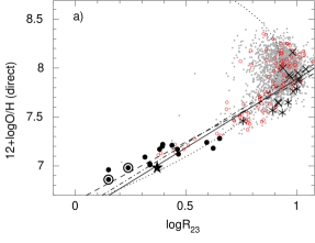
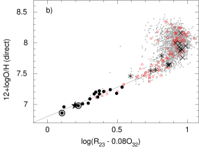
Figure 1: a) (logR₂₃) - (12 + logO/H), and b) log(R₂₃ – 0.08O₃₂) - (12 + logO/H) relations. In both these relations 12 + logO/H is derived by the direct method, R₂₃ = ([O iii]$\lambda$4959+$\lambda$5007+[O ii]$\lambda$3727)/H$\beta$ and O₃₂ = [O iii]$\lambda$5007/[O ii]$\lambda$3727. The galaxy J0811$+$4730 with the lowest luminosity-weighted oxygen abundance (Izotov et al. 2018a) is shown by a filled star, while two knots in SBS 0335$-$052W with similar or lower oxygen abundances (Izotov et al. 2009) are represented by encircled filled circles. Other lowest-metallicity SFGs from Izotov et al. (2018a), the galaxy Little Cub (Hsyu et al. 2017) and the H ii region DDO 68 #7 (Annibali et al. 2019) are shown by filled circles. SFGs with the highest O₃₂ ratios in the range $\sim$ 20 – 40 (Izotov et al. 2017) are shown by asterisks. Samples of SFGs used for the He abundance determination (Izotov et al. 2014a, and references therein) and Lyman continuum leakers (Izotov et al. 2018b, and references therein) are shown by open circles and crosses, respectively. Grey dots represent SDSS SFGs at $z$ $>$ 0.02 from DR9 and earlier releases and at any redshift from DR10 and later releases, with the [O iii] $\lambda$4363Å emission line measured with an accuracy better than 25%. The dashed, dotted, solid, and dash-dotted lines in a) are the empirical relations by Skillman (1989), Nagao et al. (2006), Yin et al. (2007) and Pilyugin (2000), respectively. The solid line in b) is the linear most likelihood fit to the SDSS data with log(R₂₃ – 0.08O₃₂) $\leq$ 0.8 (this paper).

2 Data

We have searched for extremely low-metallicity galaxies from a sample of $\sim$ 30000 SFGs selected from the spectroscopic database of the SDSS DR14 (Abolfathi et al. 2018). This is a continuation of studies which used earlier SDSS Data Releases and were published by Izotov et al. (2012) and Guseva et al. (2015, 2017). Details of SDSS sample selection can be found in Izotov et al. (2014a). This sample includes SFGs with equivalent widths EW(H$\beta$) $\ga$ 10 $\AA$ of the H$\beta$ emission line in their spectra indicating an active star formation and the presence of hot massive stars. The [O iii] $\lambda$4363 $\AA$ emission line is present in spectra of $\sim$ 18700 out of $\sim$ 30000 SFGs. In $\sim$ 2000 SDSS spectra this line is measured with an accuracy better than 25% allowing for the reliable determination of element abundances, most often of oxygen, neon and nitrogen.

The line fluxes and their errors in each spectrum were measured using the iraf splot routine and then corrected for extinction. The internal extinction was derived from the Balmer hydrogen emission line fluxes after correction for the Milky Way extinction. The line fluxes were corrected for both reddening (Cardelli et al. 1989) and underlying hydrogen stellar absorption by the application of an iterative procedure (Izotov et al. 1994) and were used for the element abundance determination. The same SDSS spectra were used for the determination of some integrated characteristics such as H$\beta$ luminosities, $L$(H$\beta$), star formation rates SFR, and stellar masses $M_{\star}$, adopting a luminosity distance derived with a cosmological calculator (NED, Wright 2006), based on the cosmological parameters $H_{0}$=67.1 km s^-1Mpc^-1, $\Omega_{\Lambda}$=0.682, and $\Omega_{m}$=0.318 (Planck Collaboration 2014).

3 Methods of oxygen abundance determinations

One of the commonly used methods of the oxygen abundance determination in low-metallicity SFGs is the direct method based on the determination of the electron temperature $T_{\rm e}$(O iii) from the [O iii] $\lambda$4363/($\lambda$4959 + $\lambda$5007) emission-line ratio and on the relation between $T_{\rm e}$(O ii) and $T_{\rm e}$(O iii) obtained by, for example, Izotov et al. (2006a) from the photoionized H ii region models. The knowledge of the temperatures and the presence of [O ii] and [O iii] emission lines in the SDSS spectra allowed us to determine the abundances of these two most abundant oxygen ions in the H ii regions and thus the total oxygen abundances for a large sample of SFGs. However, the [O iii]$\lambda$4363 $\AA$ emission line is weak in most SDSS spectra of low-metallicity SFGs and is detected with low signal-to-noise ratio introducing large uncertainties in the determination of the electron temperature and oxygen abundance.

Therefore, for these galaxies, other methods based on strong emission lines are needed to more reliably derive their metallicities. In this paper we have developed a purely empirical strong-line method based on the SDSS DR14 sample aiming to apply it for selection of the extremely low-metallicity SFG candidates. This method uses the spectroscopic properties of well-studied lowest-metallicity galaxies and is calibrated with the direct method. For the strong-line method the most natural is to use the emission-line fluxes of oxygen, the most abundant heavy element. The common approach in the past was to use the relation between the metallicity and the sum of the fluxes of strong oxygen lines in the optical range, R₂₃ = ([O ii]$\lambda$3727 + [O iii]$\lambda$4959 + [O iii]$\lambda$5007)/H$\beta$.

The problem with this method is that the relation between the metallicity and R₂₃ consists of low- (12 + logO/H $\la$ 8.0) and high-metallicity (12 + logO/H $\ga$ 8.0) branches and thus the same value of R₂₃ corresponds to two metallicities (e.g. Pagel et al. 1980; Edmunds & Pagel 1984; McGaugh 1991). Therefore, other constraints separating low- and high-metallicity branches are needed to resolve this ambiguity. One of the possible solutions is to use the relation between the metallicities and [N ii]$\lambda$6584/H$\alpha$ emission line flux ratios which monotonically increase with metallicity and thus this relation is not degenerate (e.g. van Zee et al. 1998; Pettini & Pagel 2004). However, the use of this relation for the determination of the oxygen abundances is limited because the [N ii]$\lambda$6584 emission line is very weak or undetected in low-metallicity galaxies with high-excitation H ii regions. We have used this line (or the upper limit of its flux) to separate low- and high-metallicity branches. Adopting [N ii]$\lambda$6584/H$\beta$ $\la$ 0.2 would then select objects located on the low-metallicity branch of the logR₂₃ – 12 + logO/H relation.

To construct the logR₂₃ – 12 + logO/H diagram we select $\sim$ 2000 SDSS DR14 SFGs in which the [O iii] $\lambda$4363 emission line is detected with an accuracy better than 25% (see Sect. 2) allowing for a reliable oxygen abundance determination (grey dots in Fig. 1a). Additionally, all these galaxies show in their spectra [O ii] $\lambda$3727 $\AA$, [O iii] $\lambda$4959 $\AA$, $\lambda$5007 $\AA$ and have [O iii] $\lambda$4959/H$\beta$ $\geq$ 0.2. These data are supplemented by various samples of SFGs with reliably detected [O iii] $\lambda$4363 $\AA$ emission lines in their spectra: a sample of extremely low-metallicity SFGs with 12 + logO/H $\leq$ 7.35 (filled symbols in Fig. 1a; Hsyu et al. 2017; Annibali et al. 2019; Izotov et al. 2018a, and references therein), a sample of SFGs with highest O₃₂ = [O iii]$\lambda$5007/[O ii]$\lambda$3727 ratios of $\sim$ 20 – 40 (asterisks in Fig. 1a; Izotov et al. 2017, and references therein), a sample of Lyman continuum leaking galaxies with O₃₂ ratios in the range $\sim$ 5 – 28 (crosses in Fig. 1a; Izotov et al. 2018b, and references therein), and a sample of SFGs used for the primordial He abundance determination (open circles in Fig. 1a; Izotov et al. 2014b, and references therein). We note that two encircled filled circles indicate the location of star-forming regions 3 and 4 in SBS 0335$-$052W (Izotov et al. 2009) with undetected [O iii] $\lambda$4363 $\AA$ line. They are shown because of their extremely low oxygen abundances, which are among the lowest known and considerably lower than the luminosity-weighted oxygen abundance 7.12 of SBS 0335$-$052W (Izotov & Thuan 2007). The electron temperatures and the oxygen abundances in these objects are derived by Izotov & Thuan (2007) using the semi-empirical method. However, we have not used them in our subsequent fitting of relations for the abundance determination. It is also worth to mention SFG J0811$+$4730 because of showing the lowest luminosity-weighted oxygen abundance 12 + logO/H = 6.98$\pm$0.02 known so far (filled star in Fig. 1a; Izotov et al. 2018a).

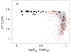
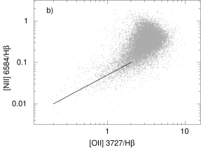
Figure 2: a) log(R₂₃ – 0.08O₃₂) - $T_{\rm e}$(O ii) relation for SFGs. b) Relation between the extinction-corrected [O ii]$\lambda$3727/H$\beta$ and [N ii]$\lambda$6584/H$\beta$ flux ratios. The solid line corresponds to [O ii]$\lambda$3727 = 20$\times$[N ii]$\lambda$6584. Symbols in both panels are as in Fig. 1.

It is important that the data include the objects with the highest O₃₂ which are indicators of a very high ionization parameter $U$ that is the measure of the number of ionizing photons per one ion in the H ii region. The use of these galaxies allows us to eliminate the dependence of the calibration relation on $U$.

For the sake of comparison, we show in Fig. 1a some simple calibration relations produced in the past. Three of them, those by Skillman (1989), Pilyugin (2000) and Yin et al. (2007), are linear. We note that these relations reproduce the oxygen abundances reasonably well (within $\sim$ 0.2 dex) of the extremely low-metallicity SFGs with log R₂₃ $<$ 0.5 shown by filled symbols. On the other hand, SFGs with highest O₃₂ at logR₂₃ $>$ 0.5 (asterisks and three SFGs shown by filled circles) considerably deviate from both the SDSS SFGs and linear relations.

We note the relatively high scatter of filled symbols in the diagram which we attribute to the ionization parameter varying in a large range. To minimize the scatter caused by various ionization parameters we show in Fig. 1b the relation log(R₂₃–0.08O₃₂) – 12 + logO/H. The distributions of SFGs in Fig. 1b show a much lower scatter than in Fig. 1a. The data in Fig. 1b can be reproduced by the linear relation

$$12+\log\frac{\rm O}{\rm H}=0.950\log({\rm R}_{23}-0.08{\rm O}_{32})+6.805,$$ (1)

shown by a solid line.

Figure 3: a) Distribution of differences between oxygen abundances 12 + logO/H derived by the semi-empirical and the direct methods for the sample from Table 2 excluding galaxies with non-detected [O iii] $\lambda$4363$\AA$ emission lines. b) As in a) but for differences between 12 + logO/H derived by our new strong-line and the direct methods. c) As in a) but for differences between 12 + logO/H derived by the strong-line and the semi-empirical methods for all SFGs from Table 2. d) As in c) but for differences between 12 + logO/H derived by the strong-line method and the strong-line method by Yin et al. (2007). e) As in c) but for differences between 12 + logO/H derived by the strong-line method and the P-method (eq. 23 in Pilyugin & Thuan 2005). f) As in c) but for differences between 12 + logO/H derived by the strong-line method and the P-method (Eq. 24 in Pilyugin & Thuan 2005). In all panels, galaxies with observed and non-observed [O ii]$\lambda$3727 emission line are shown by filled and open circles, respectively. Solid horizontal lines indicate average abundance differences and dotted horizontal lines indicate $\pm$1$\sigma$ dispersions of the sample around the average values.

4 Selection of candidates to the extremely low-metallicity SFGs in SDSS DR14

We applied Eq. 1 for selection of candidates to the extremely low-metallicity SFGs with 12 + logO/H $<$ 7.4. It is seen in Fig. 1b that these low metallicities correspond to (R₂₃ – 0.08O₃₂) $\la$ 4. We also adopted an upper limit of [N ii]$\lambda$6584/H$\beta$ $\leq$ 0.2 to exclude the contamination of the sample from objects on the upper branch of the logR₂₃ – 12 + logO/H relation, and put a low limit [O iii]$\lambda$4959/H$\beta$ $\ga$ 0.2 to exclude the galaxies which were not tested in Sect. 3 with the direct method because of the very weak [O iii]$\lambda$4363 $\AA$ emission line.

The [O ii] $\lambda$3727 $\AA$, [O iii] $\lambda$4959 $\AA$, $\lambda$5007 $\AA$ emission line intensities are needed to derive 12 + logO/H by the strong-line method discussed in Sect. 3. However, most of SDSS lowest-metallicity galaxies are at low redshifts. Therefore, the [O ii] $\lambda$3727 $\AA$ emission line is outside the wavelength range of $\sim$ 3800 – 9200 $\AA$ in spectra of galaxies with $z$ $\la$ 0.02 selected in DR9 and earlier releases, precluding the determination of metallicity while spectra of DR10 and later releases are obtained in a larger wavelength range of $\sim$ 3600 – 10300 $\AA$ including the rest-frame wavelength of [O ii] $\lambda$3727 $\AA$ emission line. To avoid this difficulty with spectra of DR9 and earlier releases some prescriptions are needed to estimate the intensity of the [O ii] $\lambda$3727 $\AA$ emission line from intensities of other lines. In particular, Izotov et al. (2012) and Guseva et al. (2015, 2017) used for that [O ii] $\lambda$7320 $\AA$, $\lambda$7330 $\AA$ emission lines. However, these lines are relatively weak or undetected introducing large uncertainties. Additionally, for galaxies at redshifts $z$ $\sim$ 0.02 – 0.03, their observed wavelengths are close to the wavelength $\sim$ 7500 $\AA$ of strong telluric absorption. Keeping in mind these caveats, we decide to use the [O ii] $\lambda$7320 $\AA$, $\lambda$7330 $\AA$ emission lines if detected for the determination of the [O ii] $\lambda$3727 $\AA$ emission line flux from the relation (Aller 1984; Izotov et al. 2006a)

$$\log I({\rm[O\leavevmode\nobreak\ II]}\lambda 3727)=0.961+\frac{8110}{T_{\rm e}({\rm O\leavevmode\nobreak\ II})}+\log I({\rm[O\leavevmode\nobreak\ II]}\lambda 7325),$$ (2)

where $I$([O ii] $\lambda$7325) = $I$([O ii] $\lambda$7320) + $I$([O ii] $\lambda$7330) and $T_{\rm e}$(O ii) is the electron temperature in the O⁺ zone of the H ii region from where [O ii] emission lines originate. Thus the electron temperature $T_{\rm e}$(O ii) is needed to derive $I$([O ii] $\lambda$3727) using Eq. 2.

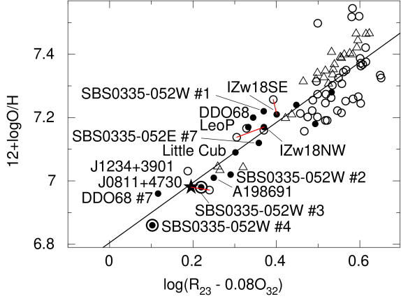
Figure 4: Log(R₂₃ – 0.08O₃₂) - (12 + logO/H) relation for SFGs with 12 + logO/H $\leq$ 7.4 from Table 2. The SFGs from the SDSS with 12 +logO/H derived by our newly introduced direct method and by the semi-empirical method are shown by open circles and open triangles, respectively. Other symbols and the solid line are the same as in Fig. 1b. Solid lines connect different observations of the same object. Some extremely low-metallicity SFGs from the literature are labelled.

Figure 5: SDSS spectra of the two lowest-metallicity galaxies represented in Table 2. Insets in both panels show expanded segments of the spectra for a better view of the [O iii] $\lambda$4363 $\AA$ emission lines.

There is no need to use Eq. 2 if [O ii] $\lambda$3727 $\AA$ is observed. If it is not observed but [O iii] $\lambda$4363 $\AA$ is detected, then both $T_{\rm e}$(O iii) and $T_{\rm e}$(O ii) can be derived. The most complicated case for SDSS spectra of low-metallicity galaxies is when both [O ii] $\lambda$3727 $\AA$ and [O iii] $\lambda$4363 $\AA$ emission lines are not detected. Then some estimates of the electron temperature $T_{\rm e}$(O ii) are needed to use the Eq. 2. To do that we consider the relation between $T_{\rm e}$(O ii) and log(R₂₃ – 0.08O₃₂) for the galaxies with spectra where the [O ii] $\lambda$3727 $\AA$ line is present and the [O iii] $\lambda$4363 $\AA$ line is detected with a relative error better than 25%. This allowed us to derive both $T_{\rm e}$(O ii) with good accuracy and R₂₃ – 0.08O₃₂. The relation is shown in Fig. 2a. It is seen that $T_{\rm e}$(O ii) at high R₂₃ – 0.08O₃₂ varies in a wide range, but it is nearly constant with the value of $\sim$ 15500 K at lower R₂₃ – 0.08O₃₂. This constancy is due to the fact that $T_{\rm e}$(O iii) at low R₂₃ – 0.08O₃₂ asymptotically approaches the value $\sim$ 22000 K. It is also worth to note that cloudy photoionization models of hottest H ii regions predict $T_{\rm e}$(O iii) and $T_{\rm e}$(O ii) of $\sim$ 22000 K – 24000 K and $\sim$ 15500 K, respectively (Ferland et al. 1998, 2013). We adopt the value $T_{\rm e}$(O ii) = 15500 K for the determination of $I$([O ii] $\lambda$3727) in the lowest-metallicity galaxy candidates for which the condition R₂₃ – 0.08O₃₂ $<$ 5 is satisfied corresponding to 12 + logO/H $\la$ 7.5.

We used the extinction-corrected [N ii]$\lambda$6584 emission line to estimate the [O ii]$\lambda$3727 emission-line flux for objects with undetected [O ii]$\lambda$7325 emission in their spectra. To find the relation between [N ii]$\lambda$6584 and [O ii]$\lambda$3727 fluxes we show in Fig. 2b the diagram [N ii]$\lambda$6584/H$\beta$ – [O ii]$\lambda$3727/H$\beta$ for SDSS DR14 SFG spectra with detected [N ii]$\lambda$6584 and [O ii]$\lambda$3727 lines. We see that

$$[{\rm OII}]\lambda 3727=20\times[{\rm NII}]\lambda 6584$$ (3)

at low [N ii]$\lambda$6584/H$\beta$ $\leq$ 0.1. The determination of the [O ii]$\lambda$3727 flux for higher [N ii]$\lambda$6584/H$\beta$ is subject to much larger uncertainties and the use of Eq. 3 would in general result in overestimation of the [O ii]$\lambda$3727 flux and correspondingly in overestimation of the oxygen abundance. We applied this relation for selection of extremely low-metallicity candidates keeping in mind that the oxygen abundance in selected SFGs with [N ii]$\lambda$6584/H$\beta$ = 0.1 – 0.2 might be overestimated. Nevertheless, additional spectroscopic observations of selected galaxies including the [O ii] $\lambda$3727 $\AA$ emission line are needed to verify and improve our indirect determination of its flux.

Three methods are used to derive the oxygen abundances. First is the direct method using prescriptions by Izotov et al. (2006a). A two-zone photoionised H ii region model was adopted: a high-ionisation zone with temperature $T_{\rm e}$(O iii), where [O iii] lines originate, and a low-ionisation zone with temperature $T_{\rm e}$(O ii), where the [O ii] lines originate. For $T_{\rm e}$(O ii), the relation between the electron temperatures $T_{\rm e}$(O iii) and $T_{\rm e}$(O ii) from Izotov et al. (2006a) is used. Ionic and total oxygen abundances are derived using expressions for oxygen ionic abundances by Izotov et al. (2006a).

The second, semi-empirical method proposed by Izotov & Thuan (2007) is based on the determination of the electron temperature from the strong oxygen emission lines in the galaxies with undetected [O iii] $\lambda$4363 $\AA$ emission line, while ionic and total oxygen abundances are derived in the way used by the direct method.

Finally, the third method is the strong-line method (Eq. 1) developed in this paper. This simplest method is purely empirical and does not require determination of physical conditions in the H ii region, at variance with the two other methods.

We selected 66 extremely low-metallicity SFGs in the entire SDSS spectroscopic data base for which at least one of the three values of 12 + logO/H derived by each of three methods is less than 7.4. The list of these SFGs is shown in Table 1 and oxygen abundances derived by all three methods to check their mutual consistency are presented in Table 2. The Tables also include coordinates, redshifts, line intensities, equivalent widths of the H$\beta$ emission line, and integrated characteristics, such as SDSS absolute magnitudes $M_{g}$ in the $g$-band and stellar masses $M_{\star}$ derived from the fitting of SDSS spectra. The selected galaxies are located mainly at very low redshifts, have faint absolute magnitudes and low stellar masses, characterising them as dwarf star-forming galaxies. The [O iii] $\lambda$4363 $\AA$ emission line is detected in most selected galaxies allowing the 12 + logO/H determination by the direct method.

A notable feature is that all three methods give consistent results with a dispersion less than 0.1 dex in most cases (Table 2). In Fig. 3 we compare oxygen abundances derived by our strong-line method with those derived by the direct, semi-empirical, and some other strong-line methods in the literature. The agreement between 12+logO/H derived with the direct method that derived with our newly developed strong-line metnod is somewhat better than that derived with the semi-empirical method. This is more clearly seen in Figs. 3a and 3b, in which we show only galaxies with detected [O iii] $\lambda$4363 $\AA$ emission line. On average, the oxygen abundances derived by the strong-line and semi-empirical methods are respectively by $\sim$ 0.04 dex and $\sim$ 0.08 dex higher than those derived by the direct method. In Fig. 3c we compare oxygen abundances derived by the strong-line and the semi-empirical methods which on average are consistent within $\sim$ 0.05 dex. The strong-line method developed in this paper and semi-empirical method are likely more preferable compared to the direct method for galaxies with weak [O iii] $\lambda$4363 $\AA$ emission, detected with poor signal-to-noise ratio.

In Fig. 3d – 3f we compare our strong-line method with some previously proposed strong-line methods from the literature. Yin et al. (2007) presented a simple relation between 12 + logO/H and R₂₃ which on average gives oxygen abundances consistent with our strong-line method (Fig. 3d). However, at lowest 12 + logO/H $\la$ 7.1, the relation by Yin et al. (2007) predicts oxygen abundances by as much as $\sim$ 0.2 higher than those obtained with our strong-line method. Pilyugin & Thuan (2005) develop their strong-line method by introducing the parameter P = [O iii]$\lambda$5007/([O ii]$\lambda$3727 + [O iii]$\lambda$5007) which takes into account the dependence on the ionization parameter. They present two relations for their method which we compare in Figs. 3e and 3f with our strong-line method. Two features of this comparison are worth to note: 1) a larger dispersion of objects compared to that in Fig. 3c and 2) a systematic offset of average values of $\Delta$(12 + logO/H) from the zero value indicating that the two modifications of the P-method give systematically higher 12 + logO/H, by $\sim$ 0.02 (Fig. 3e) and by $\sim$ 0.10 (Fig. 3f). Finally, we note that there is no difference between the galaxies with observed and non-observed [O ii] $\lambda$3727 emission line in all panels of Fig. 3 (filled and open circles, respectively) implying reliability of calculated intensities of this line. From the above comparison we conclude that our simple strong-line method is likely the most reliable for the oxygen abundance determination of extremely low-metallicity galaxies.

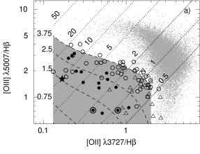
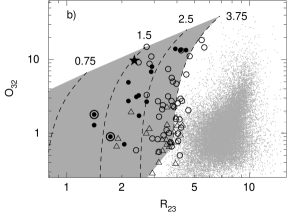
Figure 6: a) Diagnostic diagram [O iii] $\lambda$5007/H$\beta$ - [O ii] $\lambda$3727/H$\beta$. Open circles and open triangles are the extremely low-metallicity SFG candidates selected in this paper with oxygen abundances derived by the direct and semi-empirical methods, respectively. Other symbols are the same as in Fig. 1. The shaded region indicates the location of the extremely low-metallicity SFGs with 12 + logO/H in the range 6.62 – 7.39. Dotted and dashed lines are the lines of constant O₃₂ and of constant R₂₃ – 0.08O₃₂ (or constant 12 + log O/H), respectively, labelled with their values. The values R₂₃ – 0.08O₃₂ = 0.75, 1.5, 2.5, and 3.75 correspond to oxygen abundances 12 + log O/H = 6.69, 6.97, 7.18, and 7.35, respectively. b) The diagram O₃₂ – R₂₃. Symbols, lines, labels and shaded region follow the definitions provided for a).

The lowest-metallicity segment of the log(R₂₃–0.08$\times$O₃₂) – 12 + logO/H relation with 66 selected extremely low-metallicity SDSS SFGs (open circles and open triangles) and some well-studied galaxies from the literature (filled symbols) is shown in Fig. 4. Some well-known, extremely low-metallicity SFGs are labelled in the figure. The oxygen abundances for all galaxies shown in the Figure are derived by 1) the direct method if the [O iii] $\lambda$4363 $\AA$ emission line is detected (open circles) or by the 2) semi-empirical method otherwise (open triangles) while the relation for the strong-line method determined by Eq. 1 is shown by the solid line. Thirty six SDSS galaxies shown in Table 2 were previously recovered by our team (e.g. Guseva et al. 2015, 2017; Izotov & Thuan 2007; Izotov et al. 2012, 2018a). Three objects, I Zw 18SE, I Zw 18NW, and J0811$+$4730, are presented in both the SDSS and comparison samples and connected by solid red lines.

It is seen in Fig. 4 that selected SDSS galaxies (open circles and open triangles) are evenly distributed around the solid line implying that our newly proposed strong-line method (Eq. 1) reasonably well reproduces galaxy metallicities. A considerable number of SFGs have 12 + logO/H lower than in the prototypical galaxy I Zw 18. Two of these galaxies, J0811$+$4730 (see also Sect. 3) and J1234$+$3901 are very close to or below the luminosity-weighted value 12 + logO/H = 7.0, representing the lowest-metallicity galaxies known so far. In fact, using Large Binocular Telescope observations that have high signal-to-noise ratio Izotov et al. (2018a) have confirmed that J0811$+$4730 has the lowest luminosity-weighted metallicity among all low-redshift SFGs with $z$ $\la$ 0.1 (Izotov et al. 2018a). We note that metallicities in regions 3 and 4 of the galaxy SBS 0335$-$052W are even lower (Izotov et al. 2009). However, the [O iii] $\lambda$4363 $\AA$ emission line is not detected in spectra of these regions and their oxygen abundances are derived by the semi-empirical method. Furthermore, two other brighter regions 2 and 1 of SBS 0335$-$052W have higher oxygen abundances (Fig. 4) indicating an abundance gradient in this galaxy. This gradient results in a higher luminosity-weighted oxygen abundance of 7.12 averaged over the entire galaxy SBS 0335$-$052W. Annibali et al. (2019) reported the very low oxygen abundance 12 + logO/H = 6.96$\pm$0.09 in the H ii region #7 of DDO 68 derived by the direct method. However, the oxygen abundance in this region is derived with low accuracy and needs to be confirmed with higher precision. Furthermore, oxygen abundances in other H ii regions of DDO 68 are considerably higher than in the region #7 (Pustilnik et al. 2005; Izotov & Thuan 2007, 2009). We note that spectra of all these regions are not present in the SDSS data base.

One of the lowest-metallicity SFGs among selected SDSS galaxies is J1234$+$3901. A single high-excitation H ii region is observed in this galaxy with an oxygen abundance of 6.98 and 7.03 derived by the strong and direct methods, respectively. The SDSS spectra of this galaxy and another lowest-metallicity galaxy J0811$+$4730 from Table 2 are shown in Fig. 5. The [O iii] $\lambda$4363 $\AA$ emission line is clearly detected in both spectra allowing the oxygen abundance determination by the direct method. The galaxy J1234$+$3901 at the redshift of 0.1330 is one of the most distant and luminous galaxies in Table 2. Additional observations with higher signal-to-noise ratio are needed to confirm the extremely low metallicity of this galaxy.

5 Diagnostic diagrams

Izotov et al. (2012, 2018a) and Guseva et al. (2017) proposed to use the Baldwin, Phillips and Terlevich (BPT) (Baldwin et al. 1981) diagnostic diagram [O iii]$\lambda$5007/H$\beta$ vs. [N ii]$\lambda$6584/H$\alpha$ for the selection of the extremely low-metallicity SFGs. They have shown that these galaxies are located in the lower-left corner of the diagram far from the main sequence of SFGs in the region defined by relations [O iii]$\lambda$5007/H$\beta$ $<$ 4 and [N ii]$\lambda$6584/H$\alpha$ $<$ 0.03 corresponding to [N ii]$\lambda$6584/H$\beta$ $<$ 0.1. However, the use of this diagram is limited because of the weakness of the [N ii] $\lambda$6584 $\AA$ emission line. In many galaxies this line is not detected. Alternatively, the diagram [O iii]$\lambda$5007/H$\beta$ vs. [O ii]$\lambda$3727/H$\beta$ can be used as the [O ii] $\lambda$3727 $\AA$ emission line in galaxies with low metallicities is approximately 20 times brighter than the [N ii] $\lambda$6584 $\AA$ emission line.

We note that the [O ii]$\lambda$3727/H$\beta$ ratio is sensitive to dust extinction. However, in low-metallicity galaxies the internal extinction is low. It is derived from the Balmer hydrogen decrement after correction of emission line intensities for the Milky Way extinction. Both extinctions are applied to obtain extinction-corrected line intensities in the [O iii]$\lambda$5007/H$\beta$ – [O ii]$\lambda$3727/H$\beta$ diagram. We show this diagram in Fig. 6a. The shaded region indicates the location of lowest-metallicity galaxies with 12 + logO/H $\leq$ 7.35. Dashed lines indicate the lines of equal R₂₃ – 0.08O₃₂ corresponding to equal metallicities according to Eq. 1. The SFGs selected in this paper and shown in Table 2 are represented in the Figure by open circles and open triangles and are located in the shaded region. The range of [O ii] $\lambda$3727/H$\beta$ $<$ 2 is somewhat larger than $\la$ 1 tested by galaxies with 12 + logO/H derived by the direct method (filled symbols in Fig. 6a). Therefore, metallicities in galaxies with [O ii] $\lambda$3727/H$\beta$ = 1 – 2 need to be confirmed with the direct method.

Additionally, for selection of extremely low-metallicity galaxies, the O₃₂ – R₂₃ diagram can be used, as proposed by Izotov et al. (2018a). This diagram for selected SDSS galaxies (open circles and open triangles) and galaxies from the comparison sample (filled symbols) is shown in Fig. 6b. Similar to the diagram in Fig. 6a these galaxies are located far from the main-sequence SFGs (grey dots). We note a wide range of O₃₂ with the highest values reaching values up to $\sim$ 15. However, most of the extremely low-metallicity SFGs have O₃₂ $<$3. The shaded region corresponds to that in Fig. 6a. It indicates the location of extremely low-metallicity SFGs with 12 + logO/H $\leq$ 7.35.

6 Conclusions

We present results of a search for the extremely low-metallicity star-forming galaxies (SFGs) from the Data Release 14 of the Sloan Digital Sky Survey (SDSS DR14). Our main results are as follows.

1. A new, simple, purely empirical strong-line method based on the [O ii] $\lambda$3727 $\AA$ and [O iii] $\lambda$4959 $\AA$, $\lambda$5007 $\AA$ emission lines is developed for the oxygen abundance determination at low metallicities and to search for such extremely low-metallicity galaxies. This method is a modification of the well-known R₂₃ method and takes into account the dependence of oxygen emission-line fluxes not only on the metallicity but also on the ionization parameter in the H ii region. We adopt that the O₃₂ = [O iii]$\lambda$5007/[O ii]$\lambda$3727 emission-line ratio serves as a measure of the ionization parameter. This method was calibrated using observations with high signal-to-noise ratios (S/N) of a large sample of SDSS galaxies with detected [O iii] $\lambda$4363 $\AA$ emission applying the direct method in combination with other samples of SFGs with reliably derived oxygen abundances via the direct method.

2. Several selection criteria were applied to build a sample of the extremely low-metallicity SFGs. First, the SDSS galaxies were preselected using a criterion [N ii]$\lambda$6584/H$\beta$ $\leq$0.2. This allows us to exclude high-metallicity objects located on the upper branch of the R₂₃ – 12 + logO/H diagram. Then, all SFGs with [O iii]$\lambda$4959/H$\beta$ $\leq$ 0.2 were excluded because the [O iii] $\lambda$4363 $\AA$ emission line was not detected in these SFGs and thus their abundances derived by the strong method were not tested by the direct method. Finally, the remaining SFGs satisfying condition R₂₃ – 0.08O₃₂ $\la$ 4, corresponding to 12 + logO/H $<$ 7.4, were included in the final list of candidates to the lowest-metallicity SFGs.

3. We selected 66 emission-line galaxies with 12 + logO/H $\leq$ 7.35 in the entire SDSS DR14 using a new strong-line method. Some selected galaxies have 12 + logO/H as low as 7.0 and therefore belong to the lowest-metallicity SFGs known so far. Results of the metallicity determination by the new strong-line method are compared with those derived by a semi-empirical method (Izotov & Thuan 2007), by a direct method, and by some strong-line methods from the literature. We find a good agreement between 12 + logO/H derived by all three first methods with deviations less than 0.1 dex, on average. The agreement with some methods selected from the literature is not as good. However, the SDSS spectra of many selected SFGs have relatively low S/N. Furthermore, in 61 percent of SFGs the [O ii] $\lambda$3727 $\AA$ emission line is outside the wavelength range of SDSS spectra because of their low redshifts $z$ $\la$ 0.02. Therefore, its fluxes were estimated from the fluxes of weak [O ii] $\lambda$7320 $\AA$, 7330 $\AA$ or [N ii] $\lambda$6584 $\AA$ emission lines. We conclude that new observations with higher S/N and including [O ii] $\lambda$3727 $\AA$ emission line are needed to confirm the low metallicity of these selected galaxies.

4. We propose the use of two diagnostic diagrams, [O iii]$\lambda$5007/H$\beta$ – [O ii]$\lambda$3727/H$\beta$ and O₃₂ – (R₂₃ – 0.08O₃₂) for the selection of the extremely low-metallicity SFGs.

Appendix A Selected extremely low-metallicity galaxies

Table 1: List of the extremely low-metallicity SDSS galaxies from the DR14

Name	Coordinates (J2000.0)		$z$a	$g$b	Name	Coordinates (J2000.0)		$z$a	$g$b
	RA	Dec				RA	Dec
J0006$+$2413	00:06:48.96	$+$24:13:06.94	0.03418	21.66	J1034$+$1546	10:34:05.40	$+$15:46:50.14	0.00410	17.64
J0015$+$0104	00:15:20.68	$+$01:04:36.99	0.00686	19.91	J1036$+$2036	10:36:39.47	$+$20:36:15.80	0.05487	21.60
J0029$-$0025	00:29:49.50	$-$00:25:39.89	0.01412	20.23	J1053$+$4713	10:53:21.33	$+$47:13:20.85	0.06796	21.84
J0042$+$3247	00:42:33.37	$+$32:47:21.01	0.14264	22.13	J1109$+$2007	11:09:09.53	$+$20:07:29.75	0.00376	17.23
J0106$+$2345	01:06:09.17	$+$23:45:33.66	0.05206	21.93	J1119$+$0935	11:19:28.09	$+$09:35:44.28	0.00360	16.43
J0107$+$0103	01:07:46.56	$+$01:03:52.06	0.00220	19.93	J1121$+$3744	11:21:46.68	$+$37:44:21.18	0.00644	17.85
J0113$+$0052	01:13:40.44	$+$00:52:39.15	0.00381	21.18	J1139$+$1917	11:39:31.78	$+$19:17:24.92	0.01145	17.69
J0122$+$0048	01:22:41.61	$+$00:48:42.00	0.05731	21.62	J1153$+$3419	11:53:28.19	$+$34:19:21.89	0.00746	18.01
J0137$+$2032	01:37:40.98	$+$20:32:46.50	0.03480	22.25	J1157$+$1713	11:57:44.11	$+$17:13:29.19	0.01267	17.81
J0143$+$1958	01:43:15.15	$+$19:58:06.10	0.00170	21.76	J1157$+$5638	11:57:54.18	$+$56:38:16.71	0.00150	16.89
J0153$+$0104	01:53:11.96	$+$01:04:40.10	0.06332	21.52	J1206$+$5007	12:06:08.53	$+$50:07:21.17	0.05137	21.76
J0207$-$0821	02:07:24.77	$-$08:21:43.60	0.01267	20.22	J1208$+$3727	12:08:09.75	$+$37:27:24.65	0.00356	17.82
J0222$-$0935	02:22:38.55	$-$09:35:35.20	0.11477	21.61	J1220$+$4915	12:20:51.61	$+$49:15:55.48	0.01226	20.88
J0223$-$0918	02:23:02.68	$-$09:18:22.40	0.05032	20.99	J1223$+$0727	12:23:58.20	$+$07:27:01.73	0.00412	17.90
J0247$-$0404	02:47:12.80	$-$04:04:31.36	0.03495	22.07	J1226$+$0952	12:26:55.72	$+$09:52:56.27	0.00330	16.93
J0314$-$0108	03:14:26.11	$-$01:08:46.55	0.02741	17.70	J1228$-$0125	12:28:45.54	$-$01:25:26.90	0.07281	22.09
J0808$+$3244	08:08:56.34	$+$32:44:19.20	0.14640	20.60	J1234$+$3901	12:34:15.70	$+$39:01:16.41	0.13297	21.92
J0811$+$4730	08:11:52.12	$+$47:30:26.24	0.04452	21.32	J1235$+$2755	12:35:52.35	$+$27:55:54.22	0.00261	15.92
J0834$+$5905	08:34:37.19	$+$59:05:35.99	0.00480	19.86	J1244$+$3212	12:44:11.17	$+$32:12:21.69	0.00220	17.97
J0859$+$3923	08:59:46.93	$+$39:23:05.64	0.00200	17.06	J1250$+$1728	12:50:31.28	$+$17:28:15.95	0.00290	16.37
J0906$+$2528	09:06:00.92	$+$25:28:11.33	0.00923	17.41	J1257$+$3341	12:57:40.55	$+$33:41:39.24	0.00300	17.43
J0911$+$3135	09:11:59.42	$+$31:35:35.93	0.00250	17.71	J1258$+$1413	12:58:40.20	$+$14:13:00.79	0.00070	16.20
J0921$+$4038	09:21:36.55	$+$40:38:53.84	0.07136	22.04	J1308$+$2002	13:08:28.41	$+$20:02:01.93	0.00495	17.54
J0934$+$5514A	09:34:02.03	$+$55:14:27.86	0.00249	16.44	J1314$+$2438	13:14:59.16	$+$24:38:39.15	0.01265	18.10
J0934$+$5514B	09:34:02.39	$+$55:14:23.20	0.00270	17.58	J1315$+$1745	13:15:56.30	$+$17:45:38.03	0.00320	15.95
J0944$+$0936	09:44:44.59	$+$09:36:49.18	0.00180	20.36	J1414$-$0208	14:14:54.13	$-$02:08:22.94	0.00512	18.00
J0945$+$3835	09:45:19.55	$+$38:35:52.90	0.07245	21.79	J1424$+$5200	14:24:19.49	$+$52:00:38.40	0.04946	22.64
J0949$+$3426	09:49:35.09	$+$34:26:16.36	0.00500	22.24	J1433$+$1544	14:33:21.29	$+$15:44:21.60	0.02027	21.48
J0950$+$3127	09:50:19.49	$+$31:27:22.24	0.00180	17.77	J1444$+$4237	14:44:12.80	$+$42:37:44.01	0.00211	21.39
J0955$+$6442	09:55:31.45	$+$64:42:50.06	0.00320	17.92	J1522$+$4201	15:22:55.55	$+$42:01:58.30	0.00194	17.48
J0956$+$2849	09:56:46.05	$+$28:49:43.78	0.00160	14.64	J1640$+$2845	16:40:21.43	$+$28:45:55.92	0.00329	17.00
J0959$+$4626	09:59:05.76	$+$46:26:50.49	0.00200	17.79	J1703$+$2126	17:03:11.59	$+$21:26:21.20	0.10171	20.21
J1000$+$3032	10:00:36.54	$+$30:32:09.78	0.00170	17.77	J2104$-$0035	21:04:55.31	$-$00:35:22.24	0.00465	18.13

^aRedshift.

^bSDSS $g$-band magnitude.

Table 2: Emission-line intensities and oxygen abundances of the extremely low-metallicity SDSS galaxies from the DR14

	Line intensitiesa							12+logO/Hb
Name	[O ii]c	[O iii]	[O iii]	[O ii]	[N ii]	$F$(H$\beta$)d	EW(H$\beta$)e	d	se	s	$M_{g}$f	log $M_{\star}$g
	3727	4959	4363	7325	6584
J0006$+$2413	0.439	0.826	0.121	…	…	3.9	39.5	7.25	7.31	7.30	$-$15.0	7.6
J0015$+$0104h	(0.898)	0.252	…	…	0.045	5.0	177.1	…	7.03	7.06	$-$15.4	4.2
J0029$-$0025	(0.959)	0.726	0.146	…	0.048	1.8	35.1	7.25	7.37	7.34	$-$14.4	6.3
J0042$+$3247h	0.804	0.733	0.100	…	…	2.4	68.0	7.22	7.34	7.32	$-$17.2	8.0
J0106$+$2345	0.223	0.652	0.063	…	…	0.4	277.0	7.17	7.11	7.12	$-$15.2	6.4
J0107$+$0103	(1.682)	0.455	…	0.056	0.144	18.5	20.6	…	7.35	7.31	$-$10.3	5.8
J0113$+$0052h	(0.680)	0.617	0.091	…	0.034	6.6	46.3	7.16	7.22	7.25	$-$12.3	5.9
J0122$+$0048h	0.548	0.856	0.100	…	…	7.2	156.0	7.22	7.36	7.33	$-$16.1	6.8
J0137$+$2032	1.293	0.559	…	…	…	0.4	26.7	…	7.34	7.31	$-$15.2	6.7
J0143$+$1958h	1.597	0.433	…	…	…	1.4	20.8	…	7.33	7.29	$-$7.8	4.4
J0153$+$0104h	0.214	1.311	0.134	…	…	8.3	229.1	7.39	7.58	7.38	$-$16.2	6.2
J0207$-$0821h	0.883	0.661	…	…	0.105	3.7	29.3	…	7.31	7.30	$-$14.2	6.9
J0222$-$0935h	0.915	0.781	0.103	…	0.099	1.9	59.5	7.26	7.39	7.36	$-$17.2	7.9
J0223$-$0918h	1.248	0.677	…	…	…	0.6	23.1	…	7.40	7.36	$-$16.0	7.5
J0247$-$0404	0.628	0.404	…	…	…	3.7	85.0	…	7.04	7.11	$-$14.1	7.0
J0314$-$0108	0.494	0.826	0.084	0.021	0.113	26.2	31.3	7.26	7.33	7.31	$-$18.9	7.3
J0808$+$3244	1.819	0.340	0.036	…	0.102	8.6	50.4	7.31	7.32	7.28	$-$18.9	8.9
J0811$+$4730h	0.187	0.570	0.088	…	…	15.5	282.0	6.97	7.02	7.03	$-$17.3	5.8
J0834$+$5905h	(0.986)	0.552	0.059	…	0.049	8.6	22.3	7.22	7.26	7.27	$-$15.6	6.7
J0859$+$3923h	(1.989)	0.438	0.086	0.065	0.091	5.9	28.3	7.35	7.41	7.34	$-$12.8	5.4
J0906$+$2528h	(1.864)	0.582	…	…	0.093	7.0	14.4	…	7.46	7.39	$-$16.2	6.7
J0911$+$3135h	(1.544)	0.519	0.058	…	0.077	8.4	16.2	7.32	7.37	7.33	$-$12.9	5.6
J0921$+$4038	0.276	1.342	0.181	…	…	7.4	300.5	7.32	7.61	7.42	$-$15.9	6.6
J0934$+$5514Ah	(0.185)	0.678	0.072	0.016	0.006	194.9	57.6	7.14	7.12	7.09	$-$14.1	6.2
J0934$+$5514Bh	(0.505)	0.557	0.045	0.014	0.014	374.6	147.7	7.26	7.12	7.18	$-$13.1	5.1
J0944$+$0936	(1.844)	0.463	0.050	0.060	0.160	7.6	18.7	7.34	7.39	7.34	$-$10.5	5.3
J0945$+$3835h	1.238	0.845	0.124	…	…	3.5	93.9	7.33	7.50	7.42	$-$16.8	6.9
J0949$+$3426	(1.280)	0.667	0.039	0.042	0.118	12.8	33.4	7.55	7.40	7.36	$-$16.2	6.0
J0950$+$3127h	(2.485)	0.416	0.071	…	0.124	2.8	12.4	7.42	7.49	7.39	$-$12.7	5.3
J0955$+$6442h	(1.339)	0.263	0.047	…	0.067	6.5	62.9	7.16	7.17	7.16	$-$12.9	5.1
J0956$+$2849h	(2.124)	0.203	…	0.070	0.071	7.6	17.8	…	7.31	7.25	$-$14.6	4.9
J0959$+$4626h	(1.486)	0.413	0.050	…	0.074	9.5	54.1	7.26	7.29	7.27	$-$12.2	5.2
J1000$+$3032h	(1.939)	0.422	…	…	0.097	3.3	16.4	…	7.39	7.33	$-$12.5	5.5
J1034$+$1546h	(1.979)	0.521	0.057	…	0.099	9.6	19.8	7.37	7.45	7.38	$-$13.9	6.0
J1036$+$2036h	0.917	0.719	0.076	…	…	2.8	83.3	7.31	7.35	7.33	$-$15.6	7.0
J1053$+$4713	0.481	1.005	0.130	…	…	5.2	92.2	7.24	7.44	7.38	$-$16.9	7.3
J1109$+$2007h	(0.685)	0.723	0.093	0.023	0.056	15.8	61.5	7.19	7.30	7.30	$-$14.1	6.1
J1119$+$0935h	(0.870)	0.613	0.058	0.029	0.069	23.2	29.8	7.27	7.27	7.28	$-$14.0	5.9
J1121$+$3744h	(1.825)	0.336	…	…	0.091	2.0	12.9	…	7.32	7.28	$-$15.2	6.4
J1139$+$1917	(1.821)	0.459	…	…	0.091	7.1	39.3	…	7.39	7.33	$-$17.1	7.3
J1153$+$3419	(1.876)	0.459	…	0.062	0.183	4.4	9.0	…	7.40	7.34	$-$15.4	6.9
J1157$+$1713	(0.994)	0.219	…	…	0.050	2.1	9.9	…	7.05	7.05	$-$17.1	7.2
J1157$+$5638	(0.297)	1.099	0.076	0.010	0.030	52.2	85.1	7.52	7.47	7.36	$-$13.3	5.2
J1206$+$5007i	0.439	0.826	0.121	…	…	7.4	218.5	7.19	7.31	7.30	$-$15.5	6.0
J1206$+$5007i	0.328	0.813	0.085	…	…	7.5	195.4	7.20	7.28	7.26	$-$15.3	6.7
J1208$+$3727h	(1.889)	0.362	…	0.062	0.083	5.3	18.7	…	7.35	7.30	$-$14.6	6.2
J1220$+$4915h	0.225	0.997	0.128	…	…	13.9	169.2	7.20	7.38	7.28	$-$13.0	5.6
J1223$+$0727	(1.347)	0.695	0.065	…	0.067	8.7	26.3	7.36	7.43	7.38	$-$13.9	5.8
J1226$+$0952	(1.374)	0.390	0.062	0.045	0.102	6.5	35.3	7.21	7.25	7.24	$-$14.2	5.4
J1228$-$0125h	1.616	0.558	…	…	0.043	1.8	107.0	…	7.40	7.35	$-$16.4	6.9
J1234$+$3901	0.131	0.650	0.069	…	…	12.4	242.0	7.03	7.07	6.98	$-$17.6	7.4
J1235$+$2755h	(1.493)	0.631	…	0.049	0.118	12.2	31.3	…	7.42	7.37	$-$7.9	5.6
J1244$+$3212h	(0.796)	0.638	0.038	0.026	0.086	23.9	7.2	7.50	7.27	7.28	$-$15.7	6.3
J1250$+$1728	(2.647)	0.194	…	…	0.132	3.7	15.2	…	7.41	7.31	$-$14.6	5.8
J1257$+$3341h	(1.741)	0.576	0.039	0.057	0.040	29.9	108.8	7.52	7.44	7.37	$-$13.8	5.4
J1258$+$1413h	(1.500)	0.469	0.068	0.049	0.073	19.0	16.3	7.27	7.33	7.30	$-$12.5	5.8

Table 2: continued. Emission-line intensities and oxygen abundances of the extremely low-metallicity SDSS galaxies from the DR14

	Line intensitiesa							12+logO/Hb
Name	[O ii]c	[O iii]	[O iii]	[O ii]	[N ii]	$F$(H$\beta$)d	EW(H$\beta$)e	d	se	s	$M_{g}$f	log $M_{\star}$g
	3727	4959	4363	7325	6584
J1308$+$2002h	(1.592)	0.676	…	…	0.080	3.6	7.3	…	7.47	7.40	$-$15.5	6.3
J1314$+$2438	(2.074)	0.277	…	…	0.104	1.9	6.2	…	7.34	7.28	$-$16.6	6.9
J1315$+$1745	(1.624)	0.647	0.070	0.053	0.145	23.3	14.8	7.38	7.46	7.39	$-$15.6	6.4
J1414$-$0208h	(1.417)	0.523	0.051	0.047	0.025	11.4	54.9	7.30	7.34	7.31	$-$14.2	6.1
J1424$+$5200	1.117	0.427	…	…	0.065	0.2	12.5	…	7.21	7.22	$-$15.9	7.1
J1433$+$1544	0.914	0.838	0.078	0.040	0.066	2.0	34.4	7.37	7.45	7.39	$-$13.5	7.1
J1444$+$4237h	(0.850)	0.833	0.100	0.028	0.049	17.9	30.2	7.27	7.41	7.37	$-$14.4	5.4
J1522$+$4201	(2.598)	0.333	…	…	0.130	4.0	18.5	…	7.47	7.37	$-$12.3	5.5
J1640$+$2845	(1.998)	0.500	…	…	0.100	3.2	32.3	…	7.44	7.37	$-$14.7	5.8
J1703$+$2126	1.816	0.425	…	…	0.077	0.7	8.9	…	7.37	7.32	$-$19.0	8.6
J2104$-$0035h	(1.171)	0.387	…	…	0.042	9.6	20.7	…	7.20	7.20	$-$14.9	6.2

^aExtinction-corrected line intensity relative to the H$\beta$ emission line intensity. Values in parentheses are calculated [O ii] $\lambda$3727 line intensities in galaxies where this line is outside the wavelength range of the SDSS spectrum.

^bs - strong line method, se - semi-empirical method, d - direct method.

^cThe value in parentheses is derived from the [O ii]7325 flux if available or from the [N ii]6584 flux otherwise.

^dObserved flux of the H$\beta$ emission line in 10^-16erg s^-1 cm^-2.

^eEquivalent width of the H$\beta$ emission line in $\AA$.

^fAbsolute SDSS $g$ magnitude.

^glog of stellar mass in log M_⊙.

^hDiscussed in Izotov & Thuan (2007), Papaderos et al. (2008), Izotov et al. (2006b, 2012, 2018a), Guseva et al. (2015, 2017).

ⁱDifferent observations of the same galaxy.