Tipping Phenomena and Points of No Return in Ecosystems: Beyond Classical Bifurcations

Abstract

We discuss tipping phenomena (critical transitions) in nonautonomous systems using an example of a bistable ecosystem model with environmental changes represented by time-varying parameters [Scheffer et al., Ecosystems, 11 (2008), pp. 275–279]. We give simple testable criteria for the occurrence of nonautonomous tipping from the herbivore-dominating equilibrium to the plant-only equilibrium using global properties of the autonomous frozen system with fixed-in-time parameters. To begin with, we use classical autonomous bifurcation analysis to identify a codimension-three degenerate Bogdanov–Takens bifurcation: the source of a dangerous subcritical Hopf bifurcation and the organizing center for bifurcation-induced tipping (B-tipping). Then, we introduce the concept of basin instability for equilibria to identify parameter paths along which genuine nonautonomous rate-induced tipping (R-tipping) occurs without crossing any classical autonomous bifurcations. We explain nonautonomous R-tipping in terms of maximal canard trajectories and produce nonautonomous tipping diagrams in the plane of the magnitude and rate of a parameter shift to uncover intriguing R-tipping tongues and wiggling tipping-tracking bifurcation curves. Discussion of nontrivial dynamics arising from the interaction between B-tipping and R-tipping identifies “points of no return” where tipping cannot be prevented by the parameter trend reversal and “points of return tipping” where tipping is inadvertently induced by the parameter trend reversal. Our results give new insight into the sensitivity of ecosystems to the magnitudes and rates of environmental change. Finally, a comparison between “tilted” saddle-node and subcritical Hopf normal forms reveals some universal tipping properties due to basin instability, a generic dangerous bifurcation, or the combination of both.

37N25, 37B55, 37GXX, 92D40

1 Introduction

Tipping points are strongly nonlinear phenomena which can be described in layman’s terms as large, sudden and often unexpected changes in the state of a system, caused by small and slow changes in the external inputs [53, 7]. The notion of a tipping point was popularized by Gladwell [21] and has since been used in a wide range of applications including climate science [35, 22, 68, 9] and ecology [53, 59, 33, 13, 61, 67, 42]. Scientists have identified interesting questions in relation to different tipping mechanisms [7, 60], generic early warning signals near a tipping point [55, 16, 57, 52], and the possibility of preventing tipping [12, 26, 14, 51, 4] that need to be addressed in more rigorous terms. For example, Article 2 of the 1992 United Nations Framework Convention on Climate Change (UNFCCC), which was later extended to become the Kyoto Protocol [1] and the current Paris Agreement [2], pointed out two critical factors—the level and the time frame for changing greenhouse gas concentrations [3]—suggesting that there are at least two tipping mechanisms of great importance to the contemporary climate. More generally, tipping phenomena can be classified by a type of instability and analyzed in more depth, although this often requires modern mathematical techniques beyond classical autonomous stability theory, such as geometric singular perturbations [68, 67], local pullback attractors [6, 5] or snapshot attractors [18, 29], and notions of finite-time stability [50, 25, 23] or transient dynamics [28]. In particular, [6] shows that much can be understood about nonautonomous tipping in one dimension from certain properties of the autonomous frozen system with fixed-in-time inputs.

In this work, we extend the discussion from [6] to a higher dimensional example from ecology [59]. This example exhibits a counterintuitive behavior that cannot be explained in terms of a classical autonomous bifurcation of the frozen system. The herbivore population thrives with a slow increase in the food growth rate but goes extinct when the food growth rate increases too fast. From an ecological perspective, the population collapse can be discussed in terms of a “vicious cycle” that is inherent to various terrestrial and aquatic ecosystems, and arises from the population growth being a nonmonotone function of the food biomass [59]. Here, we view the population collapse as a genuine nonautonomous bifurcation. In the spirit of [6], we propose a framework that uses the global property of basin boundaries in the autonomous frozen system with fixed-in-time inputs to give criteria for the occurrence of such genuine nonautonomous bifurcations in the system with time-varying inputs. This framework should be easily accessible to applied scientists and gives new insight into nontrivial tipping phenomena in general.

Earlier mathematical models described tipping points as classical dangerous bifurcations of the frozen system that occur at critical levels of an input parameter [64, 31]. Such bifurcations have a discontinuity in the branch of exponentially stable states (attractors) at the bifurcation point, which explains why a system can remain near one stable state up to a critical level but is destined to transition to a different state past the critical level [65]. However, tipping points are not just classical autonomous bifurcations. Some systems have critical rates of parameter change, meaning that they are very sensitive to how fast external conditions or inputs change. Such systems can tip to a different state, despite the absence of any classical autonomous bifurcations, when the input parameter varies slowly but fast enough [68, 62, 59, 38, 4]. Ashwin et al. used the framework of nonautonomous dynamical systems to identify three different tipping mechanisms [7]. Bifurcation-induced tipping (B-tipping) occurs when the changing parameter passes through a critical level or a classical dangerous bifurcation of the frozen system, at which point the stable state loses stability or simply disappears. In other words, B-tipping describes the adiabatic effects of a parameter change. Rate-induced tipping (R-tipping) occurs when the parameter changes faster than some critical rate and the system deviates from the moving stable state (attractor) sufficiently far to cross some tipping threshold, e.g., the boundary of the basin of attraction. In other words, R-tipping describes the nontrivial nonadiabatic effects of a parameter change. Noise-induced tipping (N-tipping) occurs when noisy fluctuations drive the system past some tipping threshold. Shi, Li, and Chen gave an alternative but similar classification of tipping mechanisms based on relative timescales of the input and of the noisy system alone [60]. Additionally, tipping points can be described as either reversible or irreversible, depending on whether the system returns to the original stable state in the long term [69]. So far, B-tipping and R-tipping have been discussed in isolation in the literature. However, real-world tipping phenomena often involve a combination of different critical factors and different tipping mechanisms. Motivated by this observation, we analyze the effects of the rate of parameter change in the ecosystem model near the two generic dangerous bifurcations of equilibria: saddle-node and subcritical Hopf bifurcations [65]. Our strategy is to

• introduce the concepts of parameter paths and basin instability for equilibria in the autonomous frozen system with fixed-in-time parameters [6, 69] to give new insight into testable criteria for genuine nonautonomous R-tipping in the system with time-varying parameters;

• complement classical autonomous bifurcation diagrams for the frozen system with new information about genuine nonautonomous R-tipping bifurcations, which are entirely due to the rate of change of the input parameters, can be very relevant in applications, but are missed by classical autonomous bifurcation analysis;

• reveal nontrivial phenomena such as multiple critical rates and points of no return that arise from B-tipping due to a dangerous autonomous bifurcation, R-tipping due to the rate of parameter change, and the interaction between the two tipping mechanisms.

Ecological models appear to be a perfect test bed for this type of study. B-tipping has been observed and studied extensively in different ecosystems [36, 46, 58, 56, 34, 35], although the concept of a “global tipping point” in the context of planetary boundaries has recently received some criticism [41]. Ecologists speak of a “regime shift” when the bifurcation is safe or explosive and of a “critical transition” when the bifurcation is dangerous [53]; we refer to [65] for the classification of bifurcations into safe, explosive, and dangerous. Similarly, there is great and rapidly growing interest in R-tipping in the context of ecological dynamics [34, 27]. To the best of our knowledge, the first examples of R-tipping were reported in ecosystems [42, 59, 68, 62, 61, 67, 43]. More precisely, R-tipping conceptualizes a failure to adapt to changing environments [48, 15], in the sense that the stable state is continuously available, but the system is unable to adjust to its changing position when the change happens too fast. This raises the interesting research question of whether tipping phenomena observed in nature are predominantly rate-induced. What is more, the related question of whether tipping can be avoided or prevented has recently received much attention in the ecosystem literature [26, 12, 14, 51]. Proper mathematical analysis of the interaction between critical levels and critical rates, or between B-tipping and R-tipping, is exactly what is needed to gain more insight into these questions. Last, there is a strong need to better understand whether ecosystems are sensitive to the magnitudes of environmental change, the rates of environmental change, or both. This is of particular importance in view of a highly variable contemporary climate, intensifying human activity, and rapidly declining resources.

The paper is organized as follows. Section 2 introduces the ecological model given by two nonautonomous ordinary differential equations and discusses the key nonlinearity. Section 3 introduces the concepts of parameter paths and moving equilibria. In section 4 we perform classical autonomous bifurcation analysis of the frozen system with fixed-in-time parameters and give simple criteria for the occurrence of B-tipping in the nonautonomous system. In section 5 we explain the vicious cycle that arises from the population growth being a nonmonotone function of the food biomass. We then introduce the concept of basin instability for equilibria in the autonomous frozen system to give testable criteria for R-tipping to occur in the nonautonomous system. We superimpose regions of basin instability on classical bifurcation diagrams to complement them with genuine nonautonomous R-tipping bifurcations. In section 6 we obtain two-dimensional nonautonomous R-tipping diagrams in the parameter plane of the rate and magnitude of parameter shift and uncover R-tipping tongues. We also describe nontrivial tipping phenomena arising from the interaction between B-tipping and R-tipping such as tipping diagrams with S-shaped nonautonomous tipping-tracking bifurcation curves and multiple critical rates. In section 7 we partition the tipping diagrams into “points of tracking,” “points of return,” “points of no return,” and “points of return tipping” to give new insight into the problem of preventing tipping by a parameter trend reversal. Finally, we discuss the interaction between B-tipping and R-tipping for modified (tilted) normal forms of the two generic dangerous bifurcations of equilibria namely saddle-node and subcritical Hopf. We show that the nonautonomous tipping diagram from section 6 appears to be typical for nonmonotone parameter shifts that cross a basin instability boundary and a generic dangerous bifurcation but then reverse. Section 8 summarises our findings.

2 The ecosystem model and its key nonlinearity

Table 1: Description of the system parameters and their values [59].

Symbol	Description	Units	Default value
$C>0$	Competition factor of plants	m2g-1d-1	0.02
$a>0$	Half-saturation constant of functional	g m-2	10
	response
$b\geq 0$	Exponent determining the reduced	m2g-1	0–0.04
	quality of food if food biomass
	is too high
$b_{c}\geq 0$	Exponent determining the predation	m2g-1	0–0.04
	efficiency of herbivores at high food
	biomass
$E>0$	Assimilation efficiency of herbivores	dimensionless	0.4
$c_{max}>0$	Maximum food intake of herbivores	d-1	1
	when $b_{c}=0$
$m>0$	Herbivore mortality rate	d-1	0–0.2
$r>0$	Maximum plant growth rate	d-1	0–2.5

We consider a simple ecosystem model, where the time evolution of plant $P\geq 0$ and herbivore $H\geq 0$ biomass concentrations is modeled using two coupled nonautonomous ordinary differential equations [59]:

(1) $$\frac{dP}{dt} =r(t)P-CP^{2}-H\,g(P),$$

(2) $$\frac{dH}{dt} =\left(E\,e^{-bP}g(P)-m(t)\right)\!H,$$

with eight parameters. We fix six of the system parameters to the values or ranges given in Table 1. To describe changing environmental conditions, we allow the plant growth rate $r(t)$ and the herbivore mortality $m(t)$, which are the two input parameters for this study, to vary smoothly and possibly nonmonotonically over time from one asymptotic value to another. For example, $r(t)$ could describe the occurrence of a wet season, owing to a weather anomaly or El Niño Southern Oscillations, or changes in resources and habitat quality. Similarly, $m(t)$ could describe a disease outbreak among herbivores. The functional response

(3) $$g(P)=c_{max}\,\dfrac{P^{2}}{P^{2}+a^{2}}\,e^{-b_{c}P}$$

is a modification of the classical monotone and strictly increasing type-III functional response $c_{max}P^{2}/(P^{2}+a^{2})$ [24] with an exponential factor $e^{-b_{c}P}$ to account for a decline in foraging at high plant biomass. The resulting nonmonotone $g(P)$, shown in Figure 1(a) for different values of predation efficiency $b_{c}$, is believed to describe a wide range of terrestrial and aquatic ecosystems; see [66, 59] and references therein. For example, rabbits graze more with faster-growing plants as long as the plants are small enough but avoid overgrown bushes for fear of predators and are unable to graze on plants that have grown too tall. Similarly, in aquatic ecosystems, phytoplankton can be heavily consumed at early life stages by herbivorous zooplankton, but higher-density phytoplankton colonies become less prone to exploration and foraging.

Figure 1: (a) The functional response $g(P)$ with dependence on $b_{c}$. (b) The key system nonlinearity: For $b+b_{c}>0$, the net per-capita herbivore growth $h(P)=(dH/dt)/H$ has optimal plant biomass $P_{opt}$ where the growth is maximal and may change sign twice at $P_{3}$ and $P_{4}$; $m=0.1$.

Our aim is to give criteria for tipping in the nonautonomous system (1)–(2) with time-varying $r(t)$ or $m(t)$ in terms of certain local and global properties of the autonomous frozen system

(4) $$\frac{dP}{dt} =rP-CP^{2}-H\,g(P),$$

(5) $$\frac{dH}{dt} =\left(E\,e^{-bP}g(P)-m\right)\!H,$$

where $r$ and $m$ are fixed-in-time input parameters.

Owing to the modified functional response (3), the frozen system (4)–(5) is a singular perturbation problem: it has a different number of equilibrium solutions for $b+b_{c}=0$ and $0<b+b_{c}\ll 1$. To see that, consider the net per-capita herbivore growth $h(P)=(dH/dt)/H$, shown in Figure 1(b), whose roots correspond to nonzero herbivore equilibrium concentrations. When $b+b_{c}=0$, the net per-capita herbivore growth is a strictly increasing function of $P$ with a single root $P_{3}$ (Figure 1(b)). However, when $0<b+b_{c}\ll 1$, the net per-capita herbivore growth has a maximum at the optimal plant biomass

$$P_{opt}\approx\left(\frac{2a^{2}}{b+b_{c}}\right)^{\!\frac{1}{3}}$$

and can have no roots at all, one double root, or two distinct roots at $P_{3}<P_{opt}$ and $P_{4}>P_{opt}$ (Figure 1(b)); see [47] for the derivation of $P_{opt}$, $P_{3}$, and $P_{4}$. This key nonlinearity underpins nonautonomous R-tipping bifurcations and arises from the decline in foraging at high plant biomass $(b_{c}>0)$, from reduced food quality at high plant biomass $(b>0)$, or from a combination of both (Figure 1(b)). Thus, we refer to $b+b_{c}$ as the nonlinearity parameter and work with different but fixed-in-time values of $b$ and $b_{c}$, as indicated in Table 1.

3 Moving equilibria and parameter paths

Typically, the position of an equilibrium $e$ for the frozen system depends on the input parameters $r$ and/or $m$. When the input parameters vary over time, $e$ changes its position in the $(P,H)$ phase space and we speak of a moving equilibrium

$$e(t):=e(r(t),m(t)),$$

also known as a quasistatic equilibrium [7]. Note that $e(t)$ is a property of the autonomous frozen system (4)–(5) and the changing environment, but it is not a solution to the nonautonomous system (1)–(2).

As the input parameters $r(t)$ and $m(t)$ evolve smoothly over time, they trace out a continuous parameter path $\Delta$ in the two-dimensional $(r,m)$ parameter plane:

$$\Delta:=\left\{(r(t),m(t)):t\in\mathbb{R}\right\}.$$

We use the notions of a moving stable equilibrium and a parameter path to discuss the differences and interactions between B-tipping and R-tipping.

4 B-tipping: Classical autonomous bifurcations

Before we analyze genuine nonautonomous R-tipping bifurcations in the original nonautonomous system (1)–(2), we perform classical autonomous bifurcation analysis of the frozen system (4)–(5) [32]. This will allow us to contrast two tipping mechanisms: B-tipping, which is due to a slow parameter drift via a classical dangerous bifurcation of the frozen system, and genuine nonautonomous R-tipping, which is entirely due to the rate of parameter change and need not involve any classical autonomous bifurcations of the frozen system. Specifically, we compute bifurcation curves in the $(r,m)$ parameter plane and uncover a codimension-three degenerate Bogdanov–Takens bifurcation: the source of a dangerous subcritical Hopf bifurcation and the organizing center for B-tipping. We say an equilibrium or a limit cycle is stable when it is exponentially stable.

4.1 Steady bifurcations of equilibria

The frozen system (4)–(5) has at most four equilibria. A trivial equilibrium $e_{1}$ and a plant-only equilibrium $e_{2}$,

$$e_{1}=(0,0),\quad e_{2}=\left(r/C,0\right),$$

exist for all parameter settings. The trivial equilibrium $e_{1}$ is a saddle with eigenvalues $\lambda_{1}=r>0$ and $\lambda_{2}=-m<0$. The plant-only equilibrium $e_{2}$ has eigenvalues $\lambda_{1}=-r<0$ and $\lambda_{2}=Ec_{max}\,e^{-(b+b_{c})r/C}/\left((a\,C/r)^{2}+1\right)-m$. Hence, $e_{2}$ is a stable node when $\lambda_{2}<0$, is a saddle when $\lambda_{2}>0$, and undergoes a transcritical or pitchfork bifurcation whenever $\lambda_{2}=0$.

The other two equilibria correspond to a stationary coexistence of plants and herbivores and satisfy the following conditions:

(6) $$H =\frac{(r-CP)(P^{2}+a^{2})}{c_{max}\,P\,e^{-b_{c}P}},$$

(7) $$h(P) =E\,c_{max}\,\frac{P^{2}e^{-(b+b_{c})P}}{P^{2}+a^{2}}-m=0.$$

Although the roots of (7) cannot be expressed in a closed form, one can take advantage of the small nonlinearity parameter $0<b+b_{c}\ll 1$ and use perturbation methods to obtain closed form approximations in terms of an asymptotic expansion in different powers of $b+b_{c}$; see [47, sect.3.1] for the details of the derivations. Regular perturbation about $b+b_{c}=0$ gives the $P$- component of the herbivore-dominating equilibrium $e_{3}$:

(8) $$P_{3}=\sqrt{\frac{a^{2}\,m}{E\,c_{max}-m}}+\frac{a^{2}\,m\,E\,c_{max}}{2\left(E\,c_{max}-m\right)^{\,2}}\,(b+b_{c})+\mathcal{O}\!\left((b+b_{c})^{2}\right),$$

where $\mathcal{O}((b+b_{c})^{2})$ is the error term of order $(b+b_{c})^{2}$ as $(b+b_{c})\to 0$, and

(9) $$e_{3}=\left(\sqrt{\dfrac{a^{2}\,m}{E\,c_{max}-m}}+\mathcal{O}(b+b_{c}),\frac{(r-CP_{3})(P_{3}^{2}+a^{2})}{c_{max}\,P_{3}\,e^{-b_{c}P_{3}}}\right).$$

Singular perturbation about $b+b_{c}=0$ using a stretched variable $\tilde{P}=(b+b_{c})P$ gives the $P$- component of the plant-dominating equilibrium $e_{4}$:

(10) $$P_{4}=\frac{\ln\!\left(E\,c_{max}/m\right)}{b+b_{c}}-\frac{a^{2}(b+b_{c})}{\left(\ln\!\left(E\,c_{max}/m\right)\!\right)^{\,2}}+\mathcal{O}\!\left((b+b_{c})^{2}\right),$$

and

(11) $$e_{4}=\left(\frac{\ln\!\left(E\,c_{max}/m\right)}{b+b_{c}}+\mathcal{O}(b+b_{c}),\frac{(r-CP_{4})(P_{4}^{2}+a^{2})}{c_{max}\,P_{4}\,e^{-b_{c}P_{4}}}\right).$$

The main advantage of the closed form approximations is the information about the dependence of the equilibrium positions on the system parameters $r$, $m$ and $(b+b_{c})$.

Next, we consider the qubic equation

(12) $$q(P)=(b+b_{c})P^{3}+a^{2}(b+b_{c})P-2\,a^{2}=0,$$

for the parameter values from Table 1, and we show as follows.

Proposition 4.1.

In the $(r,m)$ parameter plane of the frozen system (4)–(5), there is a transcritical bifurcation curve

(13) $$T=\left\{(r,m):r\in\mathbb{R}_{+}\setminus\{CP^{*}\},\,m=\frac{E\,c_{max}e^{-(b+b_{c})r/C}}{(a\,C/r)^{2}+1}\right\}.$$

If (12) has a root $P^{*}>0$, then there is a half-line of saddle-node bifurcations

(14) $$S_{e}=\left\{(r,m):r>CP^{*},\;m=\dfrac{E\,c_{max}\,e^{-(b+b_{c})P^{*}}}{(a/P^{*})^{2}+1}\right\}$$

and a pitchfork bifurcation point

$$Pf=\left\{(r,m):r=CP^{*},\;m=\frac{E\,c_{max}e^{-(b+b_{c})P^{*}}}{(a/P^{*})^{2}+1}\right\}.$$

Proof of Proposition 4.1. Equilibrium $e_{3}$ or $e_{4}$ becomes degenerate with equilibrium $e_{2}$ in a transverse crossing if $P=r/C$ in Eqs. (6)–(7). The crossing corresponds to a codimension-one transcritical bifurcation or to a codimension-two (due to the lack of the $\mathbb{Z}_{2}$-symmetry) pitchfork bifurcation. Thus, substituting $P=r/C$ into (7) defines the curve $T$ of transcritical bifurcations in the $(r,m)$ parameter plane that may include pitchfork bifurcation points. Equilibria $e_{3}$ and $e_{4}$ become degenerate in a quadratic (saddle-node) or cubic (pitchfork) tangency when $r$-independent (7) has a positive repeated root, meaning that

(15) $$h(P)=0\;\text{ and }\;h^{\prime}(P)=0\;\text{ for some}\;P>0.$$

One can verify that the second equation in (15) holds if and only if the cubic equation (12) holds. Since $q^{\prime}(P)\geq 0$ and $q(0)<0,h^{\prime}(P)$ can have at most one positive root $P=P^{*}$. This root is used in (7) to determine the value of $m$ at which $e_{3}$ and $e_{4}$ become degenerate. To eliminate a triple degeneracy involving $e_{1}$ or $e_{2}$, we require that the corresponding $H$ from (6) is positive, meaning that $r>CP^{*}$. Thus, conditions (15) together with $r>CP$ define the half-line $S_{e}$ of saddle-node bifurcations of equilibria in the $(r,m)$ parameter plane. Finally, note that curves $T$ and $S_{e}$ meet at the point $Pf$, which corresponds to a cubic tangency of $h(P)$ or a triple degeneracy of $e_{2}$, $e_{3}$, and $e_{4}$. This is a pitchfork bifurcation point. $\blacksquare$

If $b+b_{c}=0$ (Figure 3(a)), then (12) has no roots, meaning that there are no saddle-node or pitchfork bifurcations of equilibria. The curve $T$ of transcritical bifurcations emerges from the origin and levels off at $m=E\,c_{max}$ for large $r$. The equilibrium $e_{3}$ that bifurcates from $e_{2}$ along $T$ exists below $T$. If $b+b_{c}>0$ (Figure 3(b)–(d)), then (12) has a unique root $P^{*}>0$ that corresponds to a unique half-line $S_{e}$ of saddle-node bifurcations. Equilibria $e_{3}$ and $e_{4}$ that are born along $S_{e}$ exist below $S_{e}$. The curve $T$ of transcritical bifurcations emerges from the origin, has a maximum $Pf$, and approaches $m=0$ from above for large $r$. Now, $T$ consists of two different branches separated by $Pf$. Equilibrium $e_{3}$, which bifurcates from $e_{2}$ along the solid branch of $T$, exists below the solid branch of $T$. In contrast, equilibrium $e_{4}$, which bifurcates from $e_{2}$ along the dashed branch of $T$, exists above the dashed branch of $T$. Equilibria $e_{2}$, $e_{3}$, and $e_{4}$ become degenerate in a pitchfork bifurcation at $Pf$.

Figure 2: One-parameter autonomous bifurcation diagrams for the frozen system (4)–(5) showing the position and stability of equilibria and limit cycles. The left column shows the $(P,H,m)$ space for (a) $r=0.5$, $(b,b_{c})=(0.025,0.025)$, (c) $r=1$, $(b,b_{c})=(0.02,0.02)$, and (e) $r=1.5$, $(b,b_{c})=(0.001,0.005)$. The right column shows the $(P,H,r)$ space for (b) $m=0.115$, $(b,b_{c})=(0.025,0.025)$, (d) $m=0.1$, $(b,b_{c})=(0.02,0.02)$, and (f) $m=0.25$, $(b,b_{c})=(0.001,0.005)$. Solid branches indicate stable solutions, dashed branches indicate unstable solutions. Projections onto the $(m,P)$ and $(r,P)$ planes are shown in gray. For the labeling of different bifurcations see Table 2.

4.2 Bifurcations of limit cycles

To reveal bifurcations of limit cycles and showcase different types of autonomous dynamics in the autonomous frozen system (4)–(5), we plot six examples of one-dimensional bifurcation diagrams in Figure 2 for two types of parameter paths. In the left column we fix $r$ and consider a range of $m\in(0,0.2]$. In the right column we fix $m$ and consider a range of $r\in(0,2]$. In addition to the transcritical $T$ and saddle-node $S_{e}$ bifurcations of equilibria identified in the previous section, there are supercritical (Figure 2(e)–(f)) and dangerous subcritical (Figure 2(b)–(c)) Hopf bifurcations $H_{e}$. Additionally, a limit cycle can connect to the saddle equilibrium $e_{4}$ and disappear in a homoclinic bifurcation $h$ (Figure 2(b)–(c) and (e)–(f)). Finally, there are saddle-node bifurcations of limit cycles discussed in the next section. For more details and background on classical autonomous bifurcation theory, we refer to [32].

Table 2: Glossary of terms for bifurcation diagrams.

Symbol	Description
$T$	Transcritical bifurcation
$S_{e}$	Saddle-node of equilibria bifurcation
$Pf$	Pitchfork bifurcation
$H_{e}$	Hopf bifurcation
$h$	Homoclinic bifurcation
$BT_{I(II)}$	Bogdanov–Takens type-I(II) bifurcation
$GH$	Generalized Hopf (Bautin) bifurcation
$S_{lc}$	Saddle-node of limit cycles bifurcation
$h_{res}$	Resonant homoclinic bifurcation
$BI$	Basin instability

Figure 3: Two-parameter autonomous bifurcation diagrams for the frozen system (4)–(5) in the $(r,m)$ parameter plane, obtained for different but fixed $(b,b_{c})$ = (a) $(0,0)$, (b) $(0.001,0.005)$, (c) $(0.005,0.01)$, (d) $(0.025,0.025)$. Bifurcations that give rise to attractors are plotted as solid curves. For the labeling of different bifurcations see Table 2.

4.3 Two-parameter autonomous bifurcation diagrams

To provide a systematic bifurcation analysis, we obtain two-dimensional $(r,m)$ bifurcation diagrams for different but fixed values of $b$ and $b_{c}$ (Figure 3). We plot codimension-one bifurcations that give rise to attractors as solid curves. To be more specific: along a solid (dashed) transcritical bifurcation, the bifurcating branch of equilibria is stable (of saddle type); along a solid (dashed) saddle-node bifurcation, a saddle collides with an attractor (repeller); and along solid (dashed) Hopf and homoclinic bifurcations, the bifurcating limit cycle is attracting (repelling). Transcritical and saddle-node bifurcations of equilibria are obtained using conditions (13) and (14), respectively. Hopf, homoclinic, and saddle-node bifurcations of limit cycles are computed using the numerical continuation software AUTO [17].

For each bifurcation diagram, we identify regions with qualitatively different dynamics and illustrate these with examples of phase portraits in the $(P,H)$ phase plane (Figure 4). It turns out that there are at least four qualitatively different $(r,m)$ bifurcation diagrams, depending on the settings of $b$ and $b_{c}$.

In the absence of the key nonlinearity, that is, when $b+b_{c}=0$ and $g(P)$ is the classical monotone type-III functional response, there are just two bifurcation curves: (solid) curve $T$ of transcritical bifurcations and (solid) curve $H_{e}$ of supercritical Hopf bifurcations (Figure 3(a)). These two curves do not interact, and they partition the $(r,m)$ parameter plane into three distinct regions with qualitatively different dynamics (Figure 4, 1–3). In particular, $H_{e}$ gives rise to a stable limit cycle in region 3, which represents a stable but oscillatory coexistence between plants and herbivores. These simple dynamics change drastically in the presence of the key nonlinearity.

Figure 4: Examples of qualitatively different $(P,H)$ phase portraits for the autonomous frozen system (4)–(5) showing (filled circles) stable equilibria, (open circles) unstable equilibria, (thick curves) limit cycles and stable/unstable invariant manifolds of saddle equilibria, and (thin curves) examples of typical trajectories. Note the stable limit cycle in regions 3 and 6, the unstable limit cycle in region 7, and the two limit cycles in region 8. See Table 3 for parameter values.

When $b+b_{c}$ becomes small but nonzero, meaning the functional response $g(P)$ becomes nonmonotone, a number of qualitative changes take place in the autonomous bifurcation diagram as expected from the singular perturbation nature of the problem. Specifically, there are three additional codimension-one bifurcation curves, and four special codimension-two bifurcation points (Figure 3(b)). Understanding the new bifurcation diagram is reminiscent of assembling a jigsaw-puzzle. First, a half-line $S_{e}$ of saddle-node bifurcations of equilibria appears. $S_{e}$ emerges from the pitchfork bifurcation point $Pf$ on $T$, where $T$ changes from solid to dashed. Second, $H_{e}$ is no longer unbounded at both ends but emerges from the Bogdanov–Takens bifurcation point $BT_{I}$ on $S_{e}$, where $S_{e}$ changes from solid to dashed. There are two possible types of Bogdanov–Takens bifurcation, and $BT_{I}$ is type-I according to the classification in [32, sect.8.4]. It is known from the unfolding of a Bogdanov–Takens bifurcation that the curve of homoclinic bifurcations $h$ must emerge from $BT_{I}$. Along $h$, the limit cycle originating from $H_{e}$ becomes a connecting orbit to the saddle equilibrium $e_{4}$ and disappears (Figure 4, $h$). Third, there is a generalized Hopf (or Bautin) bifurcation point $GH$ on $H_{e}$, where $H_{e}$ changes from (solid) supercritical to (dashed) subcritical [32, sect.8.3]. It is known from the unfolding of a generalized Hopf bifurcation that the curve of a saddle-node of a limit cycles $S_{lc}$ must emerge from $GH$. Along solid $S_{lc}$, two limit cycles of which one is attracting and the other repelling collide and disappear. Finally, $S_{lc}$ terminates on $h$ at a resonant homoclinic bifurcation point $h_{res}$, where $h$ changes from solid to dashed. This new bifurcation structure has five additional regions 4–8 with qualitatively different dynamics.

When the combination of $b$ and $b_{c}$ is increased further, points $GH$ and $h_{res}$ approach $BT_{I}$ (Figure 3(c)). In the process, region 3 with stable self-sustained oscillations disappears, while the bistable region 5 becomes noticeably larger. Then, there are special combinations of $b$ and $b_{c}$, where $GH$ and $h_{res}$ collide simultaneously with $BT_{I}$ and disappear in a codimension-three degenerate Bogdanov–Takens bifurcation (not shown in the figure) [47, sect.3.2.1]. This collision eliminates $S_{lc}$ together with the (dashed) supercritical part of $H_{e}$ and with regions 6 and 8. Concurrently, the Bogdanov–Takens bifurcation point changes to type-II. The difference from $BT_{I}$ is that $H_{e}$ and $h$ emerging from $BT_{II}$ swap their relative positions and become (dashed) subcritical (Figure 3(d)).

Table 3: Parameter values chosen for phase portraits in Figure 4

Phase portrait	$r$	$m$	$b$	$b_{c}$
1	0.5	0.14	0.025	0.025
2	0.5	0.05	0.025	0.025
3	1.5	0.23	0.001	0.005
4	1	0.125	0.025	0.025
5	1	0.075	0.025	0.025
6	1	0.21	0.005	0.01
7	1	0.12	0.025	0.025
8	1.5	0.18025	0.005	0.01
$h$	1.5	0.2684	0.001	0.005

Past the special combination of $b$ and $b_{c}$, there are four bifurcation curves, including the two dangerous bifurcations of equilibria that are of interest for B-tipping: the (solid) half-line $S_{e}$ of saddle-node bifurcations, and the (dashed) curve $H_{e}$ of subcritical Hopf bifurcations. Now, there are two special bifurcation points: the pitchfork point $Pf$ and a type-II Bogdanov–Takens bifurcation point $BT_{II}$. $H_{e}$ gives rise to a repelling limit cycle in region 7, which becomes a connecting orbit to the saddle equilibrium $e_{4}$ and disappears in a homoclinic bifurcation along $h$. Finally, a substantial part of the diagram is occupied by adjacent regions 5 and 7 with bistability between the plant-only equilibrium $e_{2}$ and the herbivore-dominating equilibrium $e_{3}$. This bistability is of interest for R-tipping from $e_{3}$ to $e_{2}$ studied in section 5.

4.4 Testable criterion for B-tipping

If a continuous parameter path $\Delta$ in the $(r,m)$ bifurcation diagram crosses a dangerous bifurcation for the autonomous frozen system (4)–(5), then there is a time-varying external input $(r(t),m(t))$ that traces out this path and gives rise to B-tipping in the nonautonomous system (1)–(2).

When $b+b_{c}=0$, we do not expect any B-tipping owing to the lack of dangerous bifurcations. However, when $b+b_{c}>0$, meaning that there is a decline in herbivore growth at high plant biomass, a number of different B-tipping mechanisms appear in the ecosystem model. The most dominant are the two generic dangerous bifurcations of equilibria, namely saddle-node and subcritical Hopf bifurcations. Figure 5 shows an example of a parameter path, denoted $\Delta_{m}$ in panel (a), that crosses a dangerous saddle-node bifurcation $S_{e}$ of the frozen system (4)–(5), together with the dynamics of the nonautonomous system (1)–(2) where $m(t)$ drifts slowly along the path (panel (b)). If the system starts near the stable equilibrium $e_{3}$ at the lower end $p_{1}$ of the path and $m(t)$ increases over time, then the nonautonomous system tracks the moving stable equilibrium $e_{3}(t)$ up to the point of the dangerous bifurcation $S_{e}$, which defines the critical level of $m$ (Figure 5(b)). As $m(t)$ passes through the bifurcation, the system undergoes a sudden and abrupt transition to the other stable equilibrium $e_{2}(t)$. This transition, called here B-tipping, is also known as a dynamic or adiabatic bifurcation [10, 49].

Figure 5: (a) Example of a parameter path $\Delta_{m}$, in the autonomous $(r,m)$ bifurcation diagram of the frozen system (4)–(5), that crosses a (dangerous) saddle-node bifurcation $S_{e}$. (b) As $m(t)$ is increased from $p_{1}=(0.5,0.12)$ along the path, the nonautonomous system (1)–(2) undergoes B-tipping from $e_{3}(t)$ to $e_{2}(t)$ as $m(t)$ passes through $S_{e}$. $b=b_{c}=0.025$, and $m(t)=0.12+0.015(\tanh(\varepsilon t)+1)/2$ with $\varepsilon=10^{-3}$.

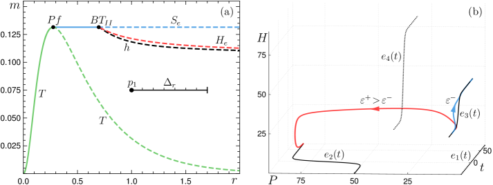
Figure 6: (a) Example of a parameter path $\Delta_{r}$, in the autonomous $(r,m)$ bifurcation diagram of the frozen system (4)–(5), that does not cross any autonomous bifurcations. (b) As $r(t)$ is increased from $p_{1}=(0.75,0.075)$ along the path at a rate $\varepsilon^{-}$ (blue trajectory) the nonautonomous system (1)–(2) tracks the moving stable equilibrium $e_{3}(t)$. However, for a faster rate $\varepsilon^{+}>\varepsilon^{-}$ (red trajectory) there is irreversible R-tipping from $e_{3}(t)$ to $e_{2}(t)$ even though $e_{3}(t)$ never disappears or loses stability in the autonomous sense. $b=b_{c}=0.025$, and $r(t)=0.75+0.6(\tanh(\varepsilon t)+1)/2$, with $\varepsilon^{-}=0.1$ and $\varepsilon^{+}=0.2$. The moving equilibria are obtained for $\varepsilon\approx 0.14$.

5 Nonautonomous R-tipping: Beyond classical autonomous bifurcations

In this section we go beyond the classical autonomous bifurcation theory and adiabatic effects of a parameter change. Specifically, we consider genuine nonautonomous bifurcations and nontrivial nonadiabatic effects of a parameter change that arise solely from the rate of change of the input parameters $r$ and $m$ and cannot be captured by classical autonomous bifurcation analysis. Specifically, we ask, Are there parameter paths in the autonomous $(r,m)$ bifurcation diagram that do not cross any bifurcation of the stable equilibrium $e_{3}$ but give rise to tipping from $e_{3}$ to $e_{2}$ when the input parameter $r$ or $m$ varies over time? The answer is yes. This was demonstrated in [59] and is examined here in more depth. Consider a parameter path $\Delta_{r}$ in Figure 6(a) that does not cross any classical autonomous bifurcations. If the nonautonomous system starts at the stable equilibrium $e_{3}$ near the lower end $p_{1}$ of the path, and $r(t)$ increases slowly enough along the path, then the nonautonomous system is able to adapt to the changing environment and track the moving stable equilibrium $e_{3}(t)$ (blue trajectory in Figure 6(b)). However, if $r(t)$ increases slowly but faster than some critical rate, the nonautonomous system fails to adapt to the changing environment and undergoes a critical transition from $e_{3}(t)$ to the other stable equilibrium $e_{2}(t)$ (red trajectory in Figure 6(b)). Tipping occurs even though $e_{3}(t)$ is continuously available and never loses stability along the path in the autonomous sense. Such a genuine nonautonomous bifurcation is known as irreversible R-tipping [7, 69].

5.1 The vicious cycle

Intuitively, R-tipping is the result of a vicious cycle that could potentially tip the system to a different state if the input parameters vary too fast. In the ecosystem model, the vicious cycle arises from the key nonlinearity, namely nonmonotone herbivore growth $h(P)=(dH/dt)/H$ that changes sign from positive to negative at high plant biomass $P=P_{4}$ (see Figure 1(b)).

The effect can be understood as follows. Consider a stable herbivore population with a lower than optimal plant biomass $P_{3}$ for some $r=r_{-}$. Then, consider a smooth increase in the plant growth rate from $r_{-}$ to $r_{+}$. This results in faster-growing plants and moves the stable equilibrium to a larger herbivore population with the same plant biomass $P_{3}$. If $r(t)$ increases slowly enough, herbivores manage to graze and grow fast enough so that the larger herbivore population is able to maintain the same plant biomass at larger $r=r_{+}$. However, if $r(t)$ increases too fast, herbivores may be unable to keep up and prevent the plant biomass from growing past its optimal value $P_{opt}$. This, in turn, triggers the vicious cycle: past the optimal plant biomass, the larger the plant biomass gets, the less the herbivores graze and grow, allowing the plant biomass to grow even larger. The ultimate effect is negative net herbivore growth causing a sudden collapse of the herbivore population. This is accompanied by a sudden increase in the plant biomass to $P_{4}$. There is no classical autonomous bifurcation along the parameter path between $r_{-}$ and $r_{+}$, but the rate of change of $r(t)$ alone prevents the system from adapting to the modified stable equilibrium. We now introduce the key mathematical concepts to analyze the vicious cycle mechanism that gives rise to genuine nonautonomous R-tipping bifurcations.

5.2 Basin instability on a path

It turns out that, similarly to B-tipping, much can be understood about genuine nonautonomous R-tipping in system (1)–(2) from certain properties of the autonomous frozen system (4)–(5) [6]. The difference is that R-tipping is related to global, rather than local, properties of the stable equilibrium. The key concept for understanding irreversible R-tipping is basin instability, and we need the following ingredients to define it:

• An exponentially stable base equilibrium $e(p)$ of the frozen system, whose position in the phase space varies with the input parameter(s) $p$. In the ecosystem model, the stable equilibrium $e_{3}$ is given in terms of $p=(r,m)$ by (9).

• Bistability or multistability in the frozen system: at least one attractor in addition to $e(p)$ for the same input parameters. The ecosystem model exhibits bistability between $e_{3}$ and $e_{2}$ in the $(r,m)$ parameter regions 5 and 7.

• A continuous parameter path $\Delta$ in the autonomous bifurcation diagram of the frozen system that does not cross any dangerous bifurcation of a stable base equilibrium $e(p)$. For example, see the path $\Delta_{r}$ in the $(r,m)$ bifurcation diagram of the ecosystem model in Figure 7(a).

• The basin of attraction of a stable base equilibrium $e(p)$ in the frozen system, defined as the set of initial states $(P_{0},H_{0})$ whose trajectories converge to $e(p)$:

  $$B(e,p)=\{(P_{0},H_{0})\in\mathbb{R}^{2}:(P(t),H(t))\to e(p),\;t\to+\infty\}.$$

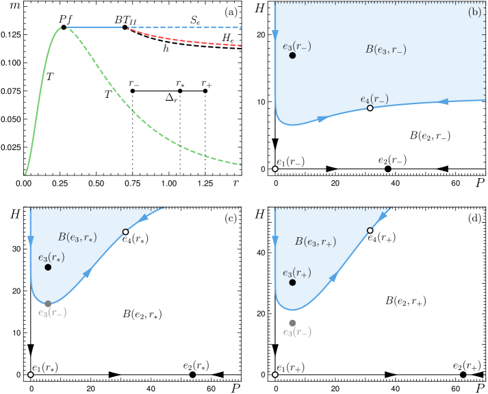
Figure 7: (a) A two-parameter autonomous bifurcation diagram for the frozen system (4)–(5) in the $(r,m)$ parameter plane with a parameter path $\Delta_{r}$ that does not cross any autonomous bifurcation. (b)–(d) Phase portraits of (4)–(5) at three different points along the path $\Delta_{r}$ illustrate basin instability of $e_{3}$ on $\Delta_{r}$. Blue shading indicates the basin of attraction of stable equilibrium $e_{3}$ for (b) $r=r_{-}=0.75$, (c) $r=r_{*}\approx 1.07672$, and (d) $r=r_{+}=1.25$. $b=b_{c}=0.025$.

Definition 5.1.

In the autonomous frozen system (4)–(5), consider a continuous parameter path $\Delta$ with a family (branch) of exponentially stable equilibria $e(p)$ that vary $C^{1}$-smoothly with $p\in\Delta$. Let $\overline{B(e,p)}$ denote the basin of attraction of $e(p)$ together with its boundary. We say that $e(p)$ is basin unstable on the path $\Delta$ if there are two points on the path $p_{1},p_{2}\in\Delta$, such that $e(p_{1})$ is outside the basin of attraction of $e(p_{2})$:

$$e(p_{1})\notin\overline{B(e,p_{2})}.$$

Note that basin instability is a global property of the autonomous frozen system and a chosen parameter path. This is illustrated for the herbivore-dominating equilibrium $e_{3}(r)$ on the path $\Delta_{r}$ in Figure 7. The stable equilibrium $e_{3}(r_{-})$ is contained within the basin of attraction of $e_{3}(r)$ for $r\in[r_{-},r_{*})$, lies on the basin boundary of $e_{3}(r_{*})$ (Figure 7(c)), and is outside the basin of attraction of $e_{3}(r)$ for $r\in(r_{*},r_{+}]$ (Figure 7(d)). Thus, $e_{3}(r)$ is basin unstable on $\Delta_{r}$. To include the global basin instability property in the classical autonomous bifurcation diagram, we make the following definition.

Definition 5.2.

In the autonomous frozen system (4)–(5), consider $e(p_{1})$ and $e(p_{2})$ from a $C^{1}$-smooth family of exponentially stable equilibria $e(p)$. We define the region of basin instability of $e(p_{1})$ as the set of points $p_{2}$ in the parameter space such that $e(p_{1})$ lies outside the basin of attraction of $e(p_{2})$:

(16) $$BI(e,p_{1})=\{p_{2}:e(p_{1})\notin\overline{B(e,p_{2})}\}.$$

The region of basin instability of the herbivore-dominating equilibrium $e_{3}(p_{1})$ in parts $5$ and $7$ of the $(r,m)$ plane, denoted $BI$ and defined as

(17) $$BI:=BI(e_{3},p_{1})=\{p_{2}\in\leavevmode\hbox to11.37pt{\vbox to11.37pt{\text{[drawing]}}}\cup\leavevmode\hbox to11.37pt{\vbox to11.37pt{\text{[drawing]}}}:e_{3}(p_{1})\notin\overline{B(e_{3},p_{2})}\},$$

is shown in gray in Figure 8(a).

We refer to [69] for extension of these ideas to threshold instability to also capture reversible R-tipping that does not require bistability or basin boundaries.

5.3 Testable criterion for R-tipping and maximal canards

Consider a continuous parameter path $\Delta$. Suppose there is a family (branch) of exponentially stable equilibria $e(p)$ of the autonomous frozen system (4)–(5) that vary $C^{1}$-smoothly with $p\in\Delta$, meaning there is no classical autonomous bifurcation of $e(p)$ on $\Delta$. If $e(p)$ is basin unstable on $\Delta$, meaning that there are points $p_{1},p_{2}\in\Delta$ such that $e(p_{1})\notin\overline{B(e,p_{2})}$, then there is a time-varying external input $p(t)=(r(t),m(t))$ that traces out the path from $p_{1}$ to $p_{2}$ and gives irreversible R-tipping from $e(t)$ in the nonautonomous system (1)–(2) [69].

It can be shown rigorously that basin instability is necessary and sufficient for the occurrence of R-tipping in one-dimensional systems [6] and sufficient but not necessary for the occurrence of R-tipping in higher-dimensional systems [69, 30, 71]. Here, we explain the rigorous results intuitively, using the example of a parameter path $\Delta_{r}$ from Figure 7. Suppose the nonautonomous system is initialized in the basin of attraction and near the stable equilibrium $e_{3}(r_{-})$, then undergoes a monotone parameter shift from $r_{-}$ to $r_{+}$. If $r(t)$ varies sufficiently slowly, the nonautonomous system is guaranteed to closely track (adiabatically follow) the moving stable equilibrium $e_{3}(t)$ along the path [6, 69]. If $r(t)$ shifts abruptly, then just after the shift, the nonautonomous system remains at its earlier position near $e_{3}(r_{-})$. This now lies outside the basin of attraction of $e_{3}(r_{+})$ and inside the basin of attraction of $e_{2}(r_{+})$ (Figure 7(d)), so the system converges to $e_{2}(r_{+})$. Thus, there must be at least one intermediate critical rate of change of $r(t)$ at which the nonautonomous tracking-tipping bifurcation occurs.

Analysis of the region of basin instability of $e_{3}(p_{1})$ in Figure 8(a) reveals that genuine nonautonomous R-tipping bifurcations are ubiquitous in the ecosystem model. They will occur on every parameter path that connects $p_{1}$ to some $p_{2}\in BI$ and stays within regions 5 and 7. Thus, in addition to dangerous magnitudes of environmental change, the ecosystem model appears to be particularly sensitive to how fast the plant growth rate $r$ increases over time. The proposed concept of basin instability quantifies this rate-of-change sensitivity and can be applied to any nonlinear system. Superimposing the region of basin instability onto a classical autonomous bifurcation diagram gives basic information on genuine nonautonomous bifurcations that can be very relevant in certain applications but are missed by classical autonomous bifurcation analysis.

One may ask about the dynamics at a critical rate, where a transition between tracking and R-tipping occurs. It turns out that, at a critical rate, the nonautonomous system somewhat surprisingly tracks the moving unstable equilibrium $e_{4}(t)$ for an infinite time (Figure 8(b)). In the terminology of slow-fast systems, a genuine nonautonomous R-tipping bifurcation corresponds to a unique maximal canard trajectory that remains within an unstable slow manifold for the longest time [63]. Depending on the basin boundary in the frozen system, critical-rate trajectories can track other moving unstable states such as limit cycles [47, Figure 5.1], which are referred to as edge states in [69]. Alternatively, a critical-rate trajectory can be transformed into a connecting (heteroclinic) orbit using the compactification technique developed in [70], as shown in [47, Chap.7] and [71].

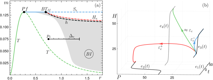
Figure 8: The same as Figure 6 but with (a) the extended path $\Delta_{r}$ and the addition of the shaded region of basin instability $BI:=BI(e_{3},p_{1})$ for $p_{1}=(0.75,0.075)$ as defined by (17), and (b) the addition of the green canard trajectory for $\varepsilon\approx\varepsilon_{c}$ that somewhat surprisingly tracks the moving unstable equilibrium $e_{4}(t)$.

6 Nonautonomous tipping diagrams for parameter shifts

Guided by the R-tipping criterion and basin instability analysis performed in the previous section, we analyze the nonautonomous system (1)–(2) with a monotone shift

(18) $$r(t)=r_{-}+\dfrac{\Delta_{r}}{2}\left(\tanh(\varepsilon t)+1\right),$$

from $r_{-}$ to $r_{+}=r_{-}+\Delta_{r}$ with $\dot{r}_{\scriptsize{max}}=\varepsilon\Delta_{r}/2$, and a nonmonotone shift

(19) $$r(t)=r_{-}+\Delta_{r}\,\mbox{sech}(\varepsilon t),$$

from $r_{-}$ to $r_{+}=r_{-}+\Delta_{r}$ and then back to $r_{-}$ with $\dot{r}_{\scriptsize{max}}=\varepsilon\Delta_{r}/2$. The shifts are parameterized by their magnitude $\Delta_{r}$ and rate $\varepsilon$, which enables parametric study in the form of two-dimensional $(\Delta_{r},\varepsilon)$ or $(\Delta_{r},\dot{r}_{max})$ nonautonomous tipping diagrams. In this way, we identify critical rates $\varepsilon_{c}$ at which the system undergoes a nonautonomous bifurcation from tracking to (irreversible) R-tipping.

6.1 Monotone shifts across a basin instability boundary: Single critical rate

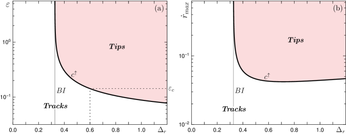
Figure 9: Nonautonomous tipping diagrams in the (a) $(\Delta_{r},\varepsilon)$ and (b) $(\Delta_{r},\dot{r}_{max})$ parameter planes for monotone shifts (18) from $p_{1}=(0.75,0.075)$ along the extended parameter path $\Delta_{r}$ from Figure 8(a). The nonautonomous tipping-tracking bifurcation curve $c^{\uparrow}$ separates the diagram into regions of (white) tracking and (pink) irreversible R-tipping. The vertical gray line indicates the boundary of the basin instability region $BI:=BI(e_{3},p_{1})$ defined by (17). The critical rate $\varepsilon_{c}$ corresponds to the (green) canard trajectory in Figure 8(b). $b=b_{c}=0.025$.

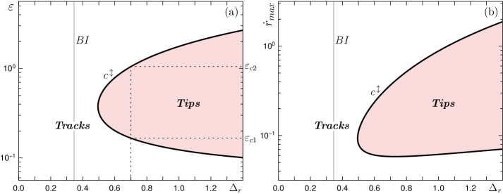
Figure 10: Nonautonomous tipping diagrams in the (a) $(\Delta_{r},\varepsilon)$ and (b) $(\Delta_{r},\dot{r}_{max})$ parameter plane for nonmonotone shifts (19) from $p_{1}=(1.0,0.075)$ along a path $\Delta_{r}$ with a fixed $m=0.075$ and varied $r>1$. The nonautonomous tipping-tracking bifurcation curve $c^{\,\updownarrow}$ separates the diagram into regions of (white) tracking and (pink) irreversible R-tipping. The vertical gray line indicates the boundary of the basin instability region $BI:=BI(e_{3},p_{1})$ defined by (17). $b=b_{c}=0.025$.

A systematic analysis of R-tipping for monotone shifts (18) from $p_{1}$ along the path $\Delta_{r}$ from Figure 8(a) gives the $(\Delta_{r},\varepsilon)$ and $(\Delta_{r},\dot{r}_{max})$ tipping diagrams in Figure 9. The nonautonomous R-tipping bifurcations occur along the curve $c^{\uparrow}$, which divides the tipping diagram into separate regions of (white) tracking and (pink) irreversible R-tipping (Figure 9). As $\Delta_{r}$ decreases, the $c^{\uparrow}$ curve becomes asymptotic to the (gray line) boundary of the basin instability region $BI$. Furthermore, the $c^{\uparrow}$ curve appears to level off at $\dot{r}_{max}\approx 0.045$. Thus, one can give simple approximate conditions for the occurrence of irreversible R-tipping along this path in terms of the shift magnitude $\Delta_{r}$ exceeding the boundary of the basin instability $BI$, and $\dot{r}_{max}$ exceeding the critical value $\approx 0.045$. Finally, the monotone shift has a unique critical rate $\varepsilon_{c}$ for a fixed magnitude $\Delta_{r}$.

6.2 Nonmonotone shifts across a basin instability boundary: Two critical rates

Analysis of R-tipping for nonmonotone shifts (19) tracing out the path $\Delta_{r}$ in Figure 8(a) from $p_{1}$ at $r_{-}=0.75$ to $r_{-}+\Delta_{r}$ and then back to $p_{1}$ is shown in the tipping diagram in Figure 10. The nonautonomous R-tipping bifurcation curve $c^{\,\updownarrow}$ forms an R-tipping tongue which is reminiscent of a resonance tongue for time-periodic inputs [40], in the sense that the system exhibits a strongly enhanced response to external inputs with optimal timing. As $\varepsilon$ is decreased from above, the natural timescales of $H(t)$ and $P(t)$ get closer to the timescale of $e_{3}(t)$, the system starts to react to the impulse input in $r$, and R-tips due to basin instability. This transition is marked by the higher critical rate $\varepsilon_{c1}$. As the natural timescales of $H(t)$ and $P(t)$ become comparable to the timescale of $e_{3}(t)$, there is a strongly enhanced response in the form of a tipping tongue. As $\varepsilon$ is decreased even further, the natural timescales of $H(t)$ and $P(t)$ become faster than the timescale of $e_{3}(t)$, and the system starts to closely track $e_{3}(t)$. This transition is marked by the lower critical rate $\varepsilon_{c1}$. The nonmonotone shift across a basin instability boundary typically has two critical rates, $\varepsilon_{c1}$ and $\varepsilon_{c2}$, for a fixed magnitude $\Delta_{r}$.

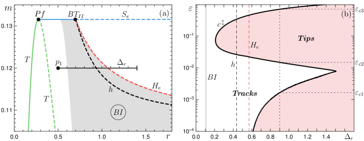
Figure 11: (a) Example of a parameter path $\Delta_{r}$, in the autonomous $(r,m)$ bifurcation diagram of the frozen system (4)–(5), that crosses the boundary of the basin instability region $BI:=BI(e_{3},p_{1})$ for $p_{1}=(0.5,0.12)$ as defined by (17), and the (dangerous) subcritical Hopf bifurcation $H_{e}$. (b) The nonautonomous tipping diagram in the $(\Delta_{m},\varepsilon)$ parameter plane for nonmonotone shift (19) from $p_{1}$ along the path $\Delta_{r}$ from panel (a). The nonautonomous tipping-tracking bifurcation curve $c^{\,\updownarrow}$ separates the diagram into regions of (white) tracking and (pink) tipping. $b=b_{c}=0.025$.

6.3 Nonmonotone shifts across a basin instability boundary and a dangerous bifurcation: A critical level and three critical rates

So far, we have discussed B-tipping and R-tipping in isolation. This and the following subsections reveal interesting tipping phenomena that arise from the interaction between B-tipping and R-tipping, or between critical levels and critical rates.

Consider nonmonotone shifts along the path $\Delta_{r}$ in Figure 11(a) from $p_{1}$, past the boundary of the basin instability $BI$, past the (dangerous) subcritical Hopf bifurcation $H_{e}$, and back to $p_{1}$. Now, the nonautonomous tipping-tracking bifurcation curve $c^{\,\updownarrow}$ consists of two distinct parts, which correspond to two different tipping mechanisms (Figure 11(b)). At high $\varepsilon$ and between $BI$ and $H_{e}$, we replicate the distinctive R-tipping tongue from Figure 10 and attribute this part to pure irreversible R-tipping. As $\varepsilon$ is decreased, there are two new features. First, the curve $c^{\,\updownarrow}$ forms a deep wedge whose tip delineates the change from R-tipping to B-tipping. Second, as $\varepsilon\to 0$, the curve $c^{\,\updownarrow}$ approaches the critical level $H_{e}$ for B-tipping, but the approach is very “slow”. The new features can be explained in terms of relative timescales and a bifurcation delay. As $\varepsilon$ decreases below the tipping tongue, the natural timescales of $H(t)$ and $P(t)$ start to exceed the timescale of $e_{3}(t)$, meaning that the system becomes more able to follow the moving stable equilibrium $e_{3}(t)$. On the one hand, we start to lose R-tipping. On the other hand, the system acquires some characteristics of a slow passage through a Hopf bifurcation. As $\varepsilon$ is decreased further, $H(t)$ and $P(t)$ become much faster than $e_{3}(t)$ and start to closely track $e_{3}(t)$. We move into the regime of a slow passage through a Hopf bifurcation, which is characterised by a noticeable bifurcation delay that does not vanish even when the rate of parameter change tends to zero [8, 44, 45]. This means that trajectories follow the moving equilibrium past the bifurcation point, where the equilibrium becomes unstable, for a noticeable time even when $\varepsilon\to 0$. Thus, the deep tracking wedge in $c^{\,\updownarrow}$ and the “slow” approach of $c^{\,\updownarrow}$ toward $H_{e}$ as $\varepsilon\to 0$ are attributed to this bifurcation delay. Finally, the change in the basin boundary at $h$, from the stable invariant manifold of the saddle $e_{4}$ to the unstable limit cycle, may be another contributing factor. In summary, the intricate tipping diagram captures different aspects of the interaction between B-tipping and R-tipping, giving rise to three critical rates.

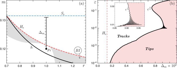
Figure 12: (a) Example of a parameter path $\Delta_{m}$, in the autonomous $(r,m)$ bifurcation diagram of the frozen system (4)–(5), that crosses the dangerous subcritical Hopf bifurcation $H_{e}$. (Gray) The basin instability region $BI:=BI(e_{3},p_{1})$ for $p_{1}=(1,0.12)$ is defined by (17). (b) The nonautonomous tipping diagram in the $(\Delta_{m},\varepsilon)$ parameter plane for nonmonotone shift (19) from $p_{1}$ along the path $\Delta_{m}$ from panel (a). The nonautonomous tipping-tracking bifurcation curve $c^{\,\updownarrow}$ separates the diagram into regions of (white) tracking and (pink) tipping. $b=b_{c}=0.025$.

6.4 Nonmonotone shifts across a dangerous bifurcation: A critical level and multiple critical rates

To reveal an interesting tipping effect that arises near a (dangerous) subcritical Hopf bifurcation, we fix $r=1$ and consider nonmonotone shifts in the herbivore death rate, $m(t)=0.12+\Delta_{m}\sinh(\varepsilon t),$ along a path $\Delta_{m}$ from Figure 12(a) that crosses a (dangerous) subcritical Hopf bifurcation $H_{e}$ with a vanishing region of basin instability.

The resulting nonautonomous tipping-tracking bifurcation curve $c^{\,\updownarrow}$ shows a complicated rate dependence that is far from trivial (Figure 12(b)). Owing to the absence of basin instability, no pure R-tipping occurs along this path. Nonetheless, there can be multiple critical rates. Past $H_{e}$, there is a range of shift magnitudes $\Delta_{m}$ with a unique critical rate. However, for larger shift magnitudes, the curve $c^{\,\updownarrow}$ has a remnant of the R-tipping tongue that gives rise to three critical rates for a fixed $\Delta_{m}$. Most interestingly, there is an interval of $\Delta_{m}$ where the wiggling part of $c^{\,\updownarrow\,}$ gives rise to several critical rates for a fixed $\Delta_{m}$ (inset in Figure 12(b)).

7 Points of return, points of no return, points of return tipping

Tipping is often defined as a large, sudden, and possibly unexpected change in the state of the system, caused by a slow or small change in the external input (e.g., environmental conditions). Although “sudden” and “unexpected” suggest that foreseeing and preventing tipping may be difficult, it should in general be possible [26]. In this section, we are guided by the question: Given a monotone parameter shift that gives tipping, under what conditions can tipping be prevented by a parameter-shift reversal? Certain aspects of this question have been explored in the context of B-tipping near a saddle-node bifurcation. For example, Hughes et al. [26] speak of “living dangerously on borrowed time” to describe a window of opportunity for ecosystems to return to safer conditions before an otherwise inevitable tipping occurs. Biggs et al. [12] ask whether early-warning indicators for tipping provide sufficient warning to modify the ecosystem’s management and avert undesired regime shifts by “turning back from the brink.” Gandhi, Knobloch, and Beaume [19, 20] consider nonmonotone parameter shifts through the (global) saddle-node on a limit cycle bifurcation to identify a new resonance mechanism in the context of spatially localized (vegetation) patterns. Ritchie, Karabacak, and Sieber [51] model systems near a saddle-node bifurcation and analyze the relationship between the time and amplitude of a saddle-node crossing to avoid B-tipping. A similar problem is analyzed by Li et al. [37] in terms of pullback attractors and points of no return. More recently, Alkhayuon et al. investigate “avoided” B-tipping and R-tipping near a subcritical Hopf bifurcation in the box model of the Atlantic Meridional Overturning Circulation (AMOC) in the context of the collapse of the AMOC and climate change mitigation [4].

Here, we extend the existing literature on avoiding B-tipping to include R-tipping effects due to basin instability. Specifically, we consider a nonautonomous system with paths in one parameter $\mu$ that may but do not need to cross a dangerous bifurcation at $\mu=\mu_{b}$. Along a path, we keep the nonmonotone shift (18) unchanged and modify the monotone shift (19) to reach a maximum in finite time:

(20) $$\mu(t)=\begin{cases}\mu_{-}+\Delta_{\mu}\,\mbox{sech}(\varepsilon t),&\,t\leq 0,\\ \mu_{-}+\Delta_{\mu},&\,t>0.\end{cases}$$

For each path, we combine nonautonomous $(\Delta_{\mu},\varepsilon)$ tipping diagrams for monotone and nonmonotone shifts to uncover four possible regions:

• Points of tracking are defined as $(\Delta_{\mu},\varepsilon)$ settings where the system avoids tipping for monotone and nonmonotone shifts. This is the safe region of tracking, sometimes referred to as the “safe operating space” [54].

• Points of return are defined as $(\Delta_{\mu},\varepsilon)$ settings where the system tips for monotone shifts, but does not tip for nonmonotone shifts. Here, an otherwise imminent tipping is prevented by the parameter-shift reversal.

• Points of no return are defined as $(\Delta_{\mu},\varepsilon)$ settings where the system tips for monotone and nonmonotone shifts. Here, tipping is not prevented by the parameter-shift reversal.

• Points of return tipping are defined as $(\Delta_{\mu},\varepsilon)$ settings where the system does not tip for monotone shifts, but tips for nonmonotone shifts. Here, the parameter-shift reversal inadvertently induces tipping in an otherwise safe situation.

Note that the existence, shape, and location of the four regions in the $(\Delta_{\mu},\varepsilon)$ tipping diagram will, in general, depend on the geometric form of the shift $\mu(t)$.

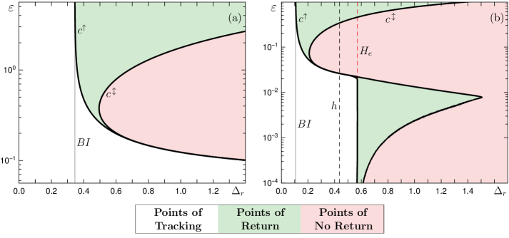
Figure 13: Nonautonomous tipping diagrams in the $(\Delta_{r},\varepsilon)$ plane for (a) R-tipping alone and (b) R- and B-tipping are partitioned into (white) “points of tracking,” (green) “points of return,” and (pink) “points of no return.” (a) The nonautonomous tipping-tracking bifurcation curves $c^{\uparrow}$ and $c^{\,\updownarrow}$ are obtained using monotone (20) and nonmonotone (19) parameter shifts, respectively, from $p_{1}=(1.0,0.075)$ along the parameter path $\Delta_{r}$ with fixed $m=0.075$ and time-varying $r>1$. (b) The nonautonomous tipping-tracking bifurcation curves $c^{\uparrow}$ and $c^{\,\updownarrow}$ are obtained using monotone (20) and nonmonotone (19) parameter shifts, respectively, from $p_{1}=(0.5,0.12)$ along the parameter path $\Delta_{r}$ from Figure 11(a). $b=b_{c}=0.025$.

7.1 The ecosystem model

For the nonautonomous ecosystem model (1)–(2), we consider two different parameter paths giving rise to two diagrams in Figure 13.

The nonautonomous $(\Delta_{r},\varepsilon)$ tipping diagram in Figure 13(a) is obtained for a parameter path with a fixed $m=0.075$, $r_{-}=1$, and $r(t)>1$ such that the path crosses the boundary of the basin instability $BI$ but does not cross any autonomous bifurcation. Points of no return are bounded by the nonautonomous R-tipping bifurcation curve $c^{\,\updownarrow}$ for the nonmonotone shift (19). Points of return are located between $c^{\,\updownarrow}$ and the nonautonomous R-tipping bifurcation curve $c^{\uparrow}$ for the monotone shift (20) with $\mu=r$. At higher $\varepsilon$, (green) points of return extend over the entire $\Delta_{r}$ interval past the boundary of $BI$. This is indicative of R-tipping occurring after the input $r(t)$ reaches its maximum. However, as $\varepsilon$ is decreased, $c^{\uparrow}$ and $c^{\,\updownarrow}$ approach each other so that the (green) points of return shrink and appear to vanish at $\varepsilon\approx 0.2$. Overlapping of $c^{\uparrow}$ and $c^{\,\updownarrow}$ gives rise to apparently direct transitions from (white) tracking to (pink) points of no return. This is indicative of R-tipping occurring before the input $r(t)$ reaches its maximum. In other words, the system R-tips from $e_{3}(t)$ to $e_{2}(t)$ during the upshift in $r(t)$, and the parameter-shift reversal has no effect on the response of the system.

The $(\Delta_{r},\varepsilon)$ tipping diagram in Figure 13(b) is obtained for the parameter path $\Delta_{r}$ from Figure 11(a) with a fixed $m=0.12$, $r_{-}=0.5$, and $r(t)>0.5$ such that the path crosses the boundary of the basin instability $BI$ as well as the (dangerous) subcritical Hopf bifurcation $H_{e}$. At higher $\varepsilon$, and between the $BI$ boundary and $H_{e}$, where R-tipping is the tipping mechanism, the diagram is the same as in Figure 13(a). At intermediate $\varepsilon$, the interplay between B-tipping and R-tipping gives rise to a deep wedge in $c^{\,\updownarrow}$, which opens up another (green) region with points of return. At lower $\varepsilon$, where B-tipping is the tipping mechanism, the (green) region with points of return shrinks but does not seem to vanish as $\varepsilon\to 0$.

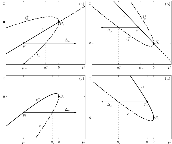
Figure 14: One-parameter bifurcation diagrams for the (tilted) subcritical Hopf normal form (21) with (a) $s>0$ and (b) $s<0$, and for the (tilted) saddle-node normal form (24) with (c) $s>0$ and (d) $s<0$. Shown are branches of (solid) stable and (dashed) unstable equilibria $e$, branches of the maxima $l_{x}^{+}$ and minima $l_{x}^{-}$ of the $x$-component of the unstable limit cycle, parameter paths $\Delta_{\mu}$ from $p_{1}=\mu_{-}$, and the corresponding boundary $\mu^{\pm}_{*}$ of the basin instability (a)–(b) $BI(e,\mu_{-})$ and (c)–(d) $BI(e^{+},\mu_{-})$.

7.2 The two generic dangerous bifurcations of equilibria

Here, we obtain nonautonomous tipping diagrams for the saddle-node and subcritical Hopf normal forms to identify typical effects of nonmonotone shifts across a dangerous bifurcation. While the normal forms are valid close to the bifurcation point, the unstable equilibrium (saddle-node) and unstable limit cycle (Hopf) do capture the global effects of the basin boundary. Furthermore, we modify the normal forms to mimic the global effects away from the bifurcation point. The main modification involves an additional parameter $s$ that “tilts” the branches of solutions in the one-parameter bifurcation diagram giving rise to basin instability; see Figure 14. There is also an additional parameter $\alpha$ that quantifies the amount of shear in the Hopf normal form.

7.2.1 Modified subcritical Hopf normal form

Consider a system in $\mathbb{R}^{2}$ akin to the normal form of a subcritical Hopf bifurcation [32, sect.3.4] written in terms of a complex variable $z=x+iy$:

(21) $$\dot{z}=\left(\mu+i\left[\omega+\alpha\left|z-\mu s\right|^{2}\right]\right)\left(z-\mu s\right)+\left|z-\mu s\right|^{2}(z-\mu s),$$

where $\mu$ is the bifurcation parameter, $\omega$ is the angular frequency of small-amplitude oscillations, $\alpha$ quantifies the amount of shear or amplitude-phase coupling, and $s$ is the “tilt” parameter. The subcritical Hopf normal form is recovered when we set $s=0$ and apply a change of coordinates to transform away the term proportional to $\alpha$ [32, sect.3.4]. There is one branch of equilibria,

$$e(\mu,s)=\mu s+0i,$$

that is stable for $\mu<0$ and unstable for $\mu>0$, and one branch of unstable limit cycles,

$$l(\mu,s,t)=\mu s+\sqrt{-\mu}\,e^{i(\omega-\alpha\mu)t},$$

that exists for $\mu<0$. The real part of the limit cycle solution oscillates between

$$l_{x}^{-}(\mu,s)=-\sqrt{-\mu}+\mu s\;\;\mbox{and}\;\;l_{x}^{+}(\mu,s)=\sqrt{-\mu}+\mu s,$$

as shown in Figure 14(a)–(b). For every $s\neq 0$, there are two basin instability boundaries:

$$\mu_{*}^{-}=\mu_{-}-\frac{1+\sqrt{1-4s^{2}\mu_{-}}}{2s^{2}}<\mu_{-}\;\;\mbox{and}\;\;\mu_{*}^{+}=\mu_{-}-\frac{1-\sqrt{1-4s^{2}\mu_{-}}}{2s^{2}}>\mu_{-}.$$

Now, consider the corresponding nonautonomous system

(22) $$\dot{z}=\left(\mu(t)+i\left[\omega+\alpha\left|z-s\,\mu(t)\right|^{2}\right]\right)\left(z-s\,\mu(t)\right)+\left|z-s\,\mu(t)\right|^{2}(z-s\,\mu(t)).$$

First, we analyze R-tipping for nonmonotone $\mu(t)$ given by (19) where we replace $r$ with $\mu$ and use $\mu_{-}=-1$ and $\Delta_{\mu}>0$ (Figure 15(a)). Tipping from the stable equilibrium $e$ requires nonzero $s$ because the branch of equilibria $e=\mu s+0i$ is flow-invariant when $s=0$. For $s=10^{-4}$, we obtain $\mu_{*}^{+}\approx-10^{-8}$, meaning that the region of basin instability between $\mu_{*}^{+}$ and $H_{e}$ is negligible. The only tipping that occurs in the nonautonomous system is B-tipping for $\Delta_{\mu}>1$, as evidenced by the tipping-tracking transition curve $c^{\,\updownarrow}$ in the $(\Delta_{\mu},\varepsilon)$ tipping diagram. When $s=0.5$, the basin instability boundary moves to $\mu_{*}^{+}=2\sqrt{2}-3\approx-0.17$ or $\Delta_{\mu}\approx 0.83$, and the region of basin instability becomes nonnegligible. As a result, the curve $c^{\,\updownarrow}$ deviates from the case $s=10^{-4}$ in different ways. While R-tipping still does not occur, basin instability gives rise to a tongue/fold on $c^{\,\updownarrow}$ and a range of shift magnitudes $\Delta_{\mu}$ with three critical rates. When the “tilt” is increased to $s=2$, the basin instability boundary moves to $\mu_{*}^{+}\approx-0.61$ or $\Delta_{\mu}\approx 0.39$. Now, in addition to B-tipping and a range of $\Delta_{\mu}$ with three critical rates, there is R-tipping for $\Delta_{\mu}<1$. The tracking-tipping transition curve $c^{\,\updownarrow}$ with the R-tipping tongue at higher rates and the “slow” approach toward $H_{e}$ as $\varepsilon\to 0$ closely resembles the tipping diagram for the ecosystem model from Figure 11(b). The most noticeable difference from the ecosystem model is the absence of the deep wedge at the intermediate rates, possibly due to the absence of the homoclinic bifurcation $h$. Instead, there is a characteristic kink on the $c^{\,\updownarrow}$ curves near $\varepsilon=10^{-2}$ in Figure 15(a) with multiple wiggles such as those shown in the inset of Figure 12(b). The origin of the kink and the wiggles, as well as the scaling law for $c^{\,\updownarrow}$ in the limit $\varepsilon\to 0$, may be related to so-called buffer points [44, 45] and are left for future study.

The same is true for “points of return” and “points of no return” shown in Figure 16(b1), where the tracking-tipping transition curve $c^{\uparrow}$ is obtained for the monotone parameter shift (20). Interestingly, for a sufficiently high “tilt” parameter $s$, a new region of “points of return tipping” appears in the diagram (Figure 16(c1)) that is not present in the ecosystem model. This means that, in general, all four regions identified in the beginning of section 7 can be present for a nonmonotone passage through a subcritical Hopf bifurcation. Furthermore, the rotational symmetry in the phase space of the (modified) Hopf normal form implies a symmetry in the basin instability boundaries

(23) $$\mu_{*}^{\pm}(s)=\mu_{*}^{\pm}(-s),$$

meaning that the system has the same basin instability properties for $s$ and $-s$. Thus, we obtain the same tipping diagrams for $s$ and $-s$ in the left column of Figure 16, in line with our R-tipping criterion from section 5.2. Finally, for a fixed $s\neq 0$, R-tipping for an increasing $\mu(t)$ requires a smaller shift magnitude than R-tipping for the decreasing $\mu(-t)$. This is why the region of “points of return tipping” in Figure 16(c1) is small.

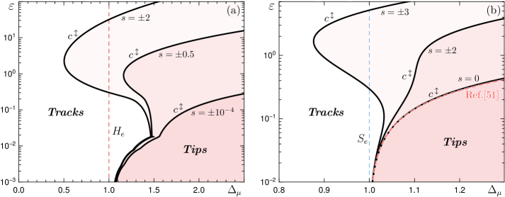
Figure 15: Nonautonomous tipping diagrams in the $(\Delta_{\mu},\varepsilon)$ parameter plane for nonmonotone shifts (19) from $p_{1}=\mu_{-}=-1$ along the parameter path $\Delta_{\mu}$ from Figure 14(a) and (c). (a) Nonautonomous tipping-tracking bifurcation curves $c^{\,\updownarrow}$ for the (tilted) subcritical Hopf normal form (22) with $\alpha=1$, $\omega=1$ and different values of $s$. (b) Nonautonomous tipping-tracking bifurcation curves $c^{\,\updownarrow}$ for the (tilted) saddle-node normal form (27) with different values of $s$. The dashed red curve in (b) is the approximation to $c^{\,\updownarrow}$ obtained in [51] for $\varepsilon s$ small enough.

7.2.2 Modified saddle-node normal form

Consider a system in $\mathbb{R}$ akin to the normal form of a saddle-node bifurcation [32, sect.3.2]:

(24) $$\dot{x}=-(x-\mu s)^{2}-\mu,$$

where $\mu$ is the bifurcation parameter and $s$ is the “tilt” parameter. The branches of stable $e^{+}$ and unstable $e^{-}$ equilibria exist for $\mu\leq 0$ and are given by

(25) $$e^{+}(\mu,s)=\mu\,s+\sqrt{-\mu},\;\;\mbox{and}\;\;e^{-}(\mu,s)=\mu\,s-\sqrt{-\mu},$$

as shown in Figure 14(c)–(d). The basin instability boundary is given by

(26) $$\mu_{*}=-\left(\sqrt{-\mu_{-}}-\frac{1}{s}\right)^{2}.$$

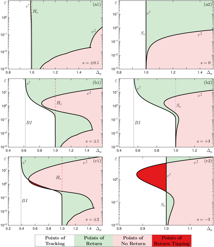
Figure 16: Nonautonomous tipping diagrams for (a1)–(c1) the (tilted) Hopf normal form (22) and (a2)–(c2) the (tilted) saddle-node normal form (22) with different values of $s$ are partitioned into (white) “points of tracking,” (green) “points of return,” (pink) “points of no return” and (red) “points of return tipping.” The nonautonomous tipping-tracking bifurcation curves $c^{\uparrow}$ and $c^{\,\updownarrow}$ are obtained for monotone (20) and nonmonotone (19) parameter shifts with $\mu_{-}=-1$ along the parameter paths $\Delta_{\mu}$ from Figure 14(a) and (c), respectively.

Now, consider the corresponding nonautonomous system

(27) $$\dot{x}=-(x-\mu(t)s)^{2}-\mu(t).$$

First, we analyze R-tipping for nonmonotone $\mu(t)$ given by (19) where we replace $r$ with $\mu$ and use $\mu_{-}=-1$ and $\Delta_{\mu}>0$ (Figure 15(b)). When $s=0$, there is no basin instability and R-tipping cannot occur [6, Theorem 3.2(1)]. The only tipping that occurs for $s=0$ is B-tipping for $\Delta_{\mu}>1$. The tracking-tipping transition curve $c^{\,\updownarrow}$ in the $(\Delta_{\mu},\varepsilon)$ tipping diagram is in very good agreement with the critical “exceedance time” inverse square law

$$t_{e}\approx\frac{2}{\sqrt{\Delta_{\mu}+\mu_{-}}},$$

derived in [51] for $\varepsilon s$ small enough. To demonstrate the agreement, we use (19) to rewrite the $t_{e}$ formula above in terms of $\varepsilon$ and $\Delta_{\mu}$,

(28) $$\varepsilon\approx\sqrt{\Delta_{\mu}+\mu_{-}}\;\mbox{sech}^{-1}\left(\frac{-\mu_{-}}{\Delta_{\mu}}\right),$$

and plot condition (28) as a dashed red curve in Figure 15(b); see [47, sect.6.2.2] for more details. However, for nonzero $s$ the tracking-tipping transition curve $c^{\,\updownarrow}$ can deviate from the inverse square law noticeably and qualitatively. When $s=2$, the tracking-tipping transition curve $c^{\,\updownarrow}$ deviates from the case $s=0$ noticeably (up to an order of magnitude in $\varepsilon$), but the changes are quantitative, and R-tipping does not occur despite crossing the basin instability boundary at $\mu_{*}=-1/4$. When the “tilt” is increased to $s=3$, the basin instability boundary moves to $\mu_{*}=-4/9$, meaning that $e^{+}$ is basin unstable for $\Delta_{\mu}>\mu_{*}-\mu_{-}=5/9$. This results in two significant changes to the tracking-tipping transition curve $c^{\,\updownarrow}$. First, $c^{\,\updownarrow}$ develops two folds and becomes S-shaped, giving rise to a range of shift magnitudes $\Delta_{\mu}$ with three different critical rates. Second, in addition to B-tipping, there is an R-tipping tongue for $\Delta_{\mu}<1$. In contrast to the subcritical Hopf bifurcation, the $c^{\,\updownarrow}$ curves clearly converge to $S_{e}$ as $\varepsilon\to 0$. This is because, as $\varepsilon\to 0$, the solution jumps off the branch of stable equilibria at the bifurcation point with no delay, meaning there is no time to turn around and avoid tipping [11, 39].

Analysis of “points of return” and “points of no return” near a saddle-node bifurcation reveals much similarity to the subcritical Hopf bifurcation when $s>0$, but not when $s<0$ (Figure 16(b2)). The striking difference for $s=-3$ is the large region of “points of return tipping,” where there is R-tipping for nonmonotone $\mu(t)$, but not for monotone increasing $\mu(t)$ (Figure 16(c2)). This difference is a consequence of asymmetry in the (modified) saddle-node normal form. To be more specific,

(29) $$\mu_{*}(s)\neq\mu_{*}(-s),$$

meaning that the system has different basin instability properties for $s$ and $-s$. According to the R-tipping criterion from section 5.2, given a suitable $\mu(t)$ that increases over time, the system is guaranteed to R-tip for $s>0$, but not for $s<0$. Conversely, given a suitable $\mu(t)$ that decreases over time, the system is guaranteed to R-tip for $s<0$, but not for $s>0$. Thus, “points of return tipping” cannot occur for $s>0$ and are expected to occur for $s<0$, which explains the diagrams for $s=3$ and $s=-3$ in Figure 16(b2) and (c2).

7.2.3 Universal properties of tipping near a dangerous bifurcation

A comparison between the tracking-tipping transition curves $c^{\,\updownarrow}$ for the modified subcritical Hopf (Figure 15(a)) and saddle-node (Figure 15(b)) normal forms reveals some universal tipping properties. In both systems, the tracking-tipping transition curve $c^{\,\updownarrow}$ becomes S-shaped, gives rise to three critical rates, and develops an R-tipping tongue as the “tilt” parameter $s$ is increased.

On the other hand, multiple critical rates and R-tipping are achieved for a smaller ‘tilt’ parameter $s$ in the modified Hopf normal form, whereas the approach of $c^{\,\updownarrow}$ toward the bifurcation as $\varepsilon\to 0$ is much faster and follows a different scaling law in the modified saddle-node normal form. Finally, owing to the different basin instability properties for $s$ and $-s$, as shown by Eqs. (23) and (29), a saddle-node bifurcation may give rise to a larger region of “points of return tipping.”

8 Conclusion

We analyze nonlinear tipping phenomena in systems with time-varying inputs, using examples of an ecological model [59] and modified saddle-node and subcritical Hopf normal forms with parameter shifts. The ecological model exhibits a somewhat counterintuitive behavior, where the herbivore population persists for a slow increase in the food growth rate but tips to extinction when the food growth rate increases too fast. We analyze such tipping phenomena as nonautonomous bifurcations. The proposed mathematical framework uses the global property of basin boundaries in the autonomous frozen system with fixed-in-time inputs to give criteria for the occurrence of nonautonomous bifurcations in the system with time-varying inputs. This framework aims to be easily accessible to applied scientists, addressing two questions of relevance: critical factors for tipping and the possibility of preventing tipping by a trend reversal. Our results give new insight into the sensitivity of ecosystems to the magnitudes and rates of environmental change.

Genuine nonautonomous rate-induced bifurcations (R-tipping), which are entirely due to the rate of change of the input parameters, are shown to correspond to maximal canard trajectories that track moving unstable states for an infinite time. We give simple criteria for the occurrence of R-tipping in the nonautonomous system using the concepts of parameter paths and basin instability on a path in the autonomous frozen system. These criteria will allow applied scientists to easily test whether their systems have critical rates of change and uncover new phenomena, such as R-tipping tongues, in the nonautonomous tipping diagrams. We also note that R-tipping problems can be transformed into connecting (heteroclinic) orbit problems using a suitable compactification technique developed in [70].

Classical autonomous bifurcation analysis of the frozen system reveals a codimension-three degenerate Bogdanov–Takens bifurcation. This is the source of a (dangerous) subcritical Hopf bifurcation and is an organizing center for bifurcation-induced tipping (B-tipping) in the nonautonomous ecosystem model. Superimposing regions of basin instability onto classical bifurcation diagrams adds information about genuine nonautonomous bifurcations, which can be even more relevant in certain applications, but are missed by classical autonomous stability analysis. Thus, our approach gives a comprehensive insight into system stability, beyond classical autonomous bifurcations and adiabatic effects of a parameter change.

Analysis of the interaction between B-tipping and R-tipping reveals an S-shaped nonautonomous bifurcation curve with multiple critical rates in the nonautonomous tipping diagram. This curve captures different tipping mechanisms, giving rise to points of tracking, points of return where tipping can be prevented by the parameter-trend reversal, points of no return where tipping cannot be prevented by the reversal, and points of return tipping where tipping is inadvertently induced by the reversal. Analysis of the modified saddle-node and subcritical Hopf normal forms suggests that these features could be considered universal for nonmonotone parameter shifts that cross a basin instability boundary and a dangerous bifurcation, and then reverses.

References

- [1] Kyoto Protocol to the United Nations Framework Convention on Climate Change, 37 I.L.M. 22 (1998); 2303 U.N.T.S. 148; U.N. Doc FCCC/CP/1997/7/Add.1, United Nations, Dec. 10, 1997.
- [2] Conference of the Parties, Adoption of the Paris Agreement, U.N. Doc. FCCC/CP/2015/L.9/Rev/1, United Nations, Dec. 12, 2015.
- [3] United Nations Framework Convention on Climate Change,1771 U.N.T.S. 107, 165; S. Treaty Doc No. 102-38 (1992); U.N. Doc. A/AC.237/18 (Part II)/Add.1; 31 I.L.M. 849 (1992), United Nations, May 9, 1992.
- [4] H. Alkhayuon, P. Ashwin, L. C. Jackson, C. Quinn, and R. A. Wood, Basin bifurcations, oscillatory instability and rate-induced thresholds for atlantic meridional overturning circulation in a global oceanic box model, Proceedings of the Royal Society A, 475 (2019), p. 20190051.
- [5] H. M. Alkhayuon and P. Ashwin, Rate-induced tipping from periodic attractors: Partial tipping and connecting orbits, Chaos: An Interdisciplinary Journal of Nonlinear Science, 28 (2018), p. 033608.
- [6] P. Ashwin, C. Perryman, and S. Wieczorek, Parameter shifts for nonautonomous systems in low dimension: bifurcation-and rate-induced tipping, Nonlinearity, 30 (2017), p. 2185.
- [7] P. Ashwin, S. Wieczorek, R. Vitolo, and P. Cox, Tipping points in open systems: bifurcation, noise-induced and rate-dependent examples in the climate system, Phil. Trans. R. Soc. A, 370 (2012), pp. 1166–1184.
- [8] S. M. Baer, T. Erneux, and J. Rinzel, The slow passage through a hopf bifurcation: delay, memory effects, and resonance, SIAM Journal on Applied mathematics, 49 (1989), pp. 55–71.
- [9] S. Bathiany, H. Dijkstra, M. Crucifix, V. Dakos, V. Brovkin, M. S. Williamson, T. M. Lenton, and M. Scheffer, Beyond bifurcation: using complex models to understand and predict abrupt climate change, Dynamics and Statistics of the Climate System, 1 (2016).
- [10] E. Benoit, Dynamics bifurcations (lecture notes in mathematics vol 1493), 1991.
- [11] N. Berglund and B. Gentz, Noise-Induced Phenomena in Slow-Fast Dynamical Systems: A Sample-Paths Approach, Springer Science & Business Media, 2006.
- [12] R. Biggs, S. R. Carpenter, and W. A. Brock, Turning back from the brink: detecting an impending regime shift in time to avert it, Proceedings of the National Academy of Sciences, 106 (2009), pp. 826–831.
- [13] C. Boettiger and A. Hastings, Tipping points: From patterns to predictions, Nature, 493 (2013), p. 157.
- [14] B. Bolt, E. H. Nes, S. Bathiany, M. E. Vollebregt, and M. Scheffer, Climate reddening increases the chance of critical transitions, Nature Climate Change, 8 (2018), p. 478.
- [15] C. A. Botero, F. J. Weissing, J. Wright, and D. R. Rubenstein, Evolutionary tipping points in the capacity to adapt to environmental change, Proceedings of the National Academy of Sciences, 112 (2015), pp. 184–189.
- [16] V. Dakos, M. Scheffer, E. H. van Nes, V. Brovkin, V. Petoukhov, and H. Held, Slowing down as an early warning signal for abrupt climate change, Proceedings of the National Academy of Sciences, 105 (2008), pp. 14308–14312.
- [17] E. J. Doedel, A. R. Champneys, T. Fairgrieve, Y. Kuznetsov, B. Oldeman, R. Paffenroth, B. Sandstede, X. Wang, and C. Zhang, Auto-07p: Continuation and bifurcation software for ordinary differential equations, Available for download from https://github.com/auto-07p/, (2007).
- [18] G. Drótos, T. Bódai, and T. Tél, Probabilistic concepts in a changing climate: A snapshot attractor picture, Journal of Climate, 28 (2015), pp. 3275–3288.
- [19] P. Gandhi, E. Knobloch, and C. Beaume, Dynamics of phase slips in systems with time-periodic modulation, Physical Review E, 92 (2015), p. 062914.
- [20] P. Gandhi, E. Knobloch, and C. Beaume, Localized states in periodically forced systems, Physical Review Letters, 114 (2015), p. 034102.
- [21] M. Gladwell, The Tipping Point: How Little Things Can Make a Big Difference, Little Brown, 2000.
- [22] H. Held and T. Kleinen, Detection of climate system bifurcations by degenerate fingerprinting, Geophysical Research Letters, 31 (2004).
- [23] L. Hoang Duc, J. Paez Chavez, D. Thai Son, and S. Siegmund, Finite-time lyapunov exponents and metabolic control coefficients for threshold detection of stimulus–response curves, Journal of Biological Dynamics, 10 (2016), pp. 379–394.
- [24] C. S. Holling, The components of predation as revealed by a study of small-mammal predation of the european pine sawfly, The Canadian Entomologist, 91 (1959), pp. 293–320.
- [25] A. Hoyer-Leitzel, A. Nadeau, A. Roberts, and A. Steyer, Detecting transient rate-tipping using steklov averages and lyapunov vectors, arXiv preprint, (2017), https://arxiv.org/abs/1702.02955.
- [26] T. P. Hughes, C. Linares, V. Dakos, I. A. Van De Leemput, and E. H. Van Nes, Living dangerously on borrowed time during slow, unrecognized regime shifts, Trends in Ecology & Evolution, 28 (2013), pp. 149–155.
- [27] T. Jezkova and J. J. Wiens, Rates of change in climatic niches in plant and animal populations are much slower than projected climate change, Proc. R. Soc. B, 283 (2016), p. 20162104.
- [28] B. Kaszás, U. Feudel, and T. Tél, Leaking in history space: A way to analyze systems subjected to arbitrary driving, Chaos: An Interdisciplinary Journal of Nonlinear Science, 28 (2018), p. 033612.
- [29] B. Kaszás, U. Feudel, and T. Tél, Tipping phenomena in typical dynamical systems subjected to parameter drift, Scientific Reports, 9 (2019), pp. 1–12.
- [30] C. Kiers and C. K. Jones, On conditions for rate-induced tipping in multi-dimensional dynamical systems, Journal of Dynamics and Differential Equations, 32 (2020), pp. 483–503.
- [31] C. Kuehn, A mathematical framework for critical transitions: Bifurcations, fast–slow systems and stochastic dynamics, Physica D: Nonlinear Phenomena, 240 (2011), pp. 1020–1035.
- [32] Y. A. Kuznetsov, Elements of Applied Bifurcation Theory, Springer, 2004.
- [33] W. F. Laurance, B. Dell, S. M. Turton, M. J. Lawes, L. B. Hutley, H. McCallum, P. Dale, M. Bird, G. Hardy, G. Prideaux, et al., The 10 australian ecosystems most vulnerable to tipping points, Biological Conservation, 144 (2011), pp. 1472–1480.
- [34] R. Leemans and B. Eickhout, Another reason for concern: regional and global impacts on ecosystems for different levels of climate change, Global Environmental Change, 14 (2004), pp. 219–228.
- [35] T. M. Lenton, H. Held, E. Kriegler, J. W. Hall, W. Lucht, S. Rahmstorf, and H. J. Schellnhuber, Tipping elements in the earth’s climate system, Proceedings of the National Academy of Sciences, 105 (2008), pp. 1786–1793.
- [36] R. C. Lewontin, The meaning of stability, Brookhaven Symposia in Biology, 22 (1969), pp. 13–24.
- [37] J. H. Li, F. X.-F. Ye, H. Qian, and S. Huang, Time-dependent saddle–node bifurcation: Breaking time and the point of no return in a non-autonomous model of critical transitions, Physica D: Nonlinear Phenomena, 395 (2019), pp. 7–14.
- [38] C. Luke and P. Cox, Soil carbon and climate change: from the jenkinson effect to the compost-bomb instability, European Journal of Soil Science, 62 (2011), pp. 5–12.
- [39] A. Majumdar, J. Ockendon, P. Howell, and E. Surovyatkina, Transitions through critical temperatures in nematic liquid crystals, Physical Review E, 88 (2013), p. 022501.
- [40] A. Marchionne, P. Ditlevsen, and S. Wieczorek, Synchronisation vs. resonance: Isolated resonances in damped nonlinear oscillators, Physica D: Nonlinear Phenomena, (2018).
- [41] J. M. Montoya, I. Donohue, and S. L. Pimm, Planetary boundaries for biodiversity: implausible science, pernicious policies, Trends in Ecology & Evolution, 33 (2018), pp. 71–73.
- [42] J. T. Morris, P. Sundareshwar, C. T. Nietch, B. Kjerfve, and D. R. Cahoon, Responses of coastal wetlands to rising sea level, Ecology, 83 (2002), pp. 2869–2877.
- [43] F. Neijnens, Rate-induced critical transitions in tidal marsh ecosystems, master’s thesis, Utrecht University, 2019.
- [44] A. Neishtadt, Persistence of stability loss for dynamical bifurcations i, Differential Equations, 23 (1987), pp. 1385–1391.
- [45] A. Neishtadt, Persistence of stability loss for dynamical bifurcations ii, Differential Equations, 24 (1988), pp. 171–176.
- [46] I. Noy-Meir, Stability of grazing systems: an application of predator-prey graphs, The Journal of Ecology, (1975), pp. 459–481.
- [47] P. E. O’Keeffe, On the Interaction of Rate-Induced and Bifurcation-Induced Tipping in Ecosystems, PhD thesis, University College Cork, 2019.
- [48] C. Perryman and S. Wieczorek, Adapting to a changing environment: non-obvious thresholds in multi-scale systems, Proceedings of the Royal Society A: Mathematical, Physical and Engineering Sciences, 470 (2014), p. 20140226.
- [49] M. Rasmussen, Attractivity and Bifurcation for Nonautonomous Dynamical Systems, Springer, 2007.
- [50] M. Rasmussen, Finite-time attractivity and bifurcation for nonautonomous differential equations, Differential Equations and Dynamical Systems, 18 (2010), pp. 57–78.
- [51] P. Ritchie, O. Karabacak, and J. Sieber, Inverse-square law between time and amplitude for crossing tipping thresholds, Proceedings of the Royal Society A, 475 (2019), p. 20180504.
- [52] P. Ritchie and J. Sieber, Early-warning indicators for rate-induced tipping, Chaos: An Interdisciplinary Journal of Nonlinear Science, 26 (2016), p. 093116.
- [53] M. Scheffer, Critical Transitions in Nature and Society, vol. 16, Princeton University Press, 2009.
- [54] M. Scheffer, S. Barrett, S. Carpenter, C. Folke, A. J. Green, M. Holmgren, T. Hughes, S. Kosten, I. Van de Leemput, D. Nepstad, et al., Creating a safe operating space for iconic ecosystems, Science, 347 (2015), pp. 1317–1319.
- [55] M. Scheffer, J. Bascompte, W. A. Brock, V. Brovkin, S. R. Carpenter, V. Dakos, H. Held, E. H. Van Nes, M. Rietkerk, and G. Sugihara, Early-warning signals for critical transitions, Nature, 461 (2009), p. 53.
- [56] M. Scheffer, S. Carpenter, J. A. Foley, C. Folke, and B. Walker, Catastrophic shifts in ecosystems, Nature, 413 (2001), p. 591.
- [57] M. Scheffer, S. R. Carpenter, T. M. Lenton, J. Bascompte, W. Brock, V. Dakos, J. Van de Koppel, I. A. Van de Leemput, S. A. Levin, E. H. Van Nes, et al., Anticipating critical transitions, Science, 338 (2012), pp. 344–348.
- [58] M. Scheffer, S. Hosper, M. Meijer, B. Moss, and E. Jeppesen, Alternative equilibria in shallow lakes, Trends in Ecology & Evolution, 8 (1993), pp. 275–279.
- [59] M. Scheffer, E. H. Van Nes, M. Holmgren, and T. Hughes, Pulse-driven loss of top-down control: the critical-rate hypothesis, Ecosystems, 11 (2008), pp. 226–237.
- [60] J. Shi, T. Li, and L. Chen, Towards a critical transition theory under different temporal scales and noise strengths, Physical Review E, 93 (2016), p. 032137.
- [61] K. Siteur, M. B. Eppinga, A. Doelman, E. Siero, and M. Rietkerk, Ecosystems off track: rate-induced critical transitions in ecological models, Oikos, 125 (2016), pp. 1689–1699.
- [62] K. Siteur, E. Siero, M. B. Eppinga, J. D. Rademacher, A. Doelman, and M. Rietkerk, Beyond turing: The response of patterned ecosystems to environmental change, Ecological Complexity, 20 (2014), pp. 81–96.
- [63] P. Szmolyan and M. Wechselberger, Canards in R3, Journal of Differential Equations, 177 (2001), pp. 419–453.
- [64] J. M. T. Thompson and J. Sieber, Predicting climate tipping as a noisy bifurcation: A review, International Journal of Bifurcation and Chaos, 21 (2011), pp. 399–423.
- [65] J. M. T. Thompson, H. Stewart, and Y. Ueda, Safe, explosive, and dangerous bifurcations in dissipative dynamical systems, Physical Review E, 49 (1994), p. 1019.
- [66] J. van de Koppel, J. Huisman, R. van der Wal, and H. Olff, Patterns of herbivory along a productivity gradient: An empirical and theoretical investigation, Ecology, 77 (1996), pp. 736–745.
- [67] A. Vanselow, S. Wieczorek, and U. Feudel, When very slow is too fast – collapse of a predator-prey system, Journal of theoretical biology, 479 (2019), pp. 64–72.
- [68] S. Wieczorek, P. Ashwin, C. M. Luke, and P. M. Cox, Excitability in ramped systems: the compost-bomb instability, Proc. R. Soc. A, 467 (2011), pp. 1243–1269.
- [69] S. Wieczorek, C. Xie, and P. Ashwin, Rate-induced tipping: Regular thresholds, edge states and testable criteria, In preparation, (2020).
- [70] S. Wieczorek, C. Xie, and C. K. R. T. Jones, Compactification for Asymptotically Autonomous Dynamical Systems: Theory, Applications and Invariant Manifolds, arXiv preprint, (2020), https://arxiv.org/abs/2001.08733.
- [71] C. Xie, Rate-Induced Critical Transitions, PhD thesis, University College Cork, 2020.