Anomalous diffusion: A basic mechanism for the evolution of inhomogeneous systems

Abstract

In this article we review classical and recent results in anomalous diffusion and provide mechanisms useful for the study of the fundamentals of certain processes, mainly in condensed matter physics, chemistry and biology. Emphasis will be given to some methods applied in the analysis and characterization of diffusive regimes through the memory function, the mixing condition (or irreversibility), and ergodicity. Those methods can be used in the study of small-scale systems, ranging in size from single-molecule to particle clusters and including among others polymers, proteins, ion channels and biological cells, whose diffusive properties have received much attention lately.

I Introduction

I.1 General concepts

Diffusion is a basic transport process involved in the evolution of many non-equilibrium systems towards equilibrium Vainstein et al. (2006a); Shlesinger et al. (1993); Metzler et al. (1999); Metzler and Klafter (2000); Morgado et al. (2002); Metzler and Klafter (2004); Sancho et al. (2004); Costa et al. (2003); Lapas et al. (2008); Weron and Magdziarz (2010); Thiel et al. (2013); McKinley and Nguyen (2018); Flekkøy (2017). By diffusion, particles (or molecules) spread from regions of high concentration to those of low concentration leading, via a gradual mixing, to a situation in which they become evenly dispersed. Diffusion is of fundamental importance in many disciplines; for example, in growth phenomena, the Edwards-Wilkinson equation is given by a diffusion equation plus a noise Barabási and Stanley (1995). In cell biology it constitutes a main form of transport for amino acids and other nutrients within cells Murray (2002).

For more than two hundred years Vainstein et al. (2006a), diffusion has been a widely studied phenomena in natural science due to it’s large number of applications. Initially, the experiments carried out by Robert Brown Brown (1828a, b) called the attention to the random trajectories of small particles of polen and also of inorganic matter. This irregular motion, later named Brownian motion, can be modeled by a random walk in which the mean square displacement is given by Einstein’s relation Vainstein et al. (2006a)

$$\langle(\Delta r)^{2}\rangle=2dDt,$$ (1)

where $\Delta r$ is the displacement of the Brownian particle in a given time interval $t$, $d$ is the spatial dimension, and $D$ the diffusion coefficient. Whereas a single Brownian particle trajectory is chaotic, averaging over many trajectories reveals a regular behavior.

The purpose of this article is to review recent efforts aiming at formulating a theory for anomalous diffusion processes– i.e., those where the mean square displacement does not follow Equation (1) which can be applied to many different situations from theoretical physics to biology.

In the next section, we introduce the pioneering works on diffusion, and then call attention to the existence of anomalous diffusion. We discuss the main methods to treat anomalous diffusion and concentrate our efforts on the discussion of the generalized Langevin formalism.

I.2 The tale of the three giants

At the birth of the gravitational theory Isaac Newton mentioned that he build up his theory based on the previous works of giants. Also, one cannot talk about diffusion without underscoring the works of Albert Einstein, Marian Smoluchowski, and Paul Langevin. At the dawn of the last century, the atomic theory was not widely accepted by the physical community. Einstein believed that the motion observed by Brown was due to the collisions of molecules such as proposed by Boltzmann in his famous equation. However, Boltzmann’s equation was difficult to solve and therefore he proposed a simpler analysis combining the kinetic theory of molecules with the Fick’s law, from which he obtained the diffusion equation

$$\frac{\partial\rho(x,t)}{\partial t}=D\,\nabla^{2}\rho(x,t),$$ (2)

where $\rho(x,t)$ is the density of particles at position $x$ and time $t$. The solution of the above equation yields $\rho(x,t)$ and

$$\lim_{t\rightarrow\infty}\langle x^{2}(t)\rangle=\int x^{2}(t)\rho(x,t)dx=2Dt,$$ (3)

where $\langle x(t)\rangle=0$, assuming the symmetry $\rho(-x,t)=\rho(x,t)$. For simplicity, we have considered the motion one-dimensional and set all particles at the origin at time $t=0$. Generalization to two and three dimensions is straightforward. He then considered the molecules as single non-interacting spherical particles with radius $a$ and mass $m$, and subject to a friction $\gamma$ when moving in the liquid Vainstein et al. (2006a); Einstein (1905, 1956) .

Finally, he deduced the famous Einstein-Stokes relation Einstein (1956) for the diffusion constant

$$D=\frac{RT}{6\pi N_{a}a\eta}=\frac{RT}{mN_{a}\gamma}=\frac{RT\mu}{N_{a}},$$ (4)

where $N_{a}$ is Avogadro’s number, fundamental for atomic theory, but unknown at the time, $R$ is the gas constant, $\mu$ the mobility, $\eta$ the viscosity, and $T$ the temperature.

The scientific community became very excited and, in the years following Einstein’s papers, some dedicated experiments helped to verify Equation (3). Diffusion constants were measured and it became possible to estimate Avogadro’s number from different experiments. Moreover, it was possible to estimate the radius of molecules with few hundreds of atoms. Einstein was successful in demonstrating that atoms and molecules were not mere illusions as critics used to suggest. Finally, the theory of Brownian motion started to set a firm ground. For instance, it became possible to associate diffusion with conductivity in the case of a gas of charged particles. Supposing each has the same charge $e$ and is subjected to a time dependent electric field $\vec{E}=\vec{{E}}(\omega)\exp(-i\omega t)$, the conductivity $\tilde{\sigma}(\omega)$ can be defined by $\vec{J}(\omega)=\tilde{\sigma}(\omega)\vec{E}(\omega)$, where $\vec{J}(\omega)$ is the current. Now, it was possible to relate the diffusivity $\tilde{D}(w)$ with $\tilde{\sigma}(\omega)$ by the relation Vainstein et al. (2006a); Dyre and Schrøder (2000); Oliveira et al. (2005)

$$\tilde{\sigma}(\omega)=\frac{ne^{2}}{k_{B}T}\widetilde{D}(\omega),$$ (5)

where is $n$ the carrier density. From that it was obvious that connections between a diversity of response functions could be obtained.

Two major achievements in the theory of stochastic motion were due to Smoluchowski. As expressed by Novak et al. Gudowska-Nowak et al. (2017), “One was the Smoluchowski equation describing the motion of a diffusive particle in an external force field, known in the Western literature as the Fokker-Planck equation Risken (1989); Salinas (2001)”

$$\begin{split}\frac{\partial P(v,t,v_{0})}{\partial t}=-\frac{\partial}{\partial v}&\left[A(v)P(v,t,v_{0})\right]\\ &+\frac{1}{2}\frac{\partial^{2}}{\partial v^{2}}\left[B(v)P(v,t,v_{0})\right],\end{split}$$ (6)

where

$$A(v)=\frac{1}{\delta t}\int_{-\infty}^{\infty}(v^{\prime}-v)P(v^{\prime},\delta t,v)\,dv^{\prime}$$ (7)

and

$$B(v)=\frac{1}{\delta t}\int_{-\infty}^{\infty}(v^{\prime}-v)^{2}P(v^{\prime},\delta t,v)\,dv^{\prime}.$$ (8)

Here $P(v^{\prime},\delta t,v)$ is the transition probability between two states with different velocities. The second one, a fundamental cornerstone of molecular physical chemistry and of cellular biochemistry Gudowska-Nowak et al. (2017); Gadomski et al. (2018) is “Smoluchowski’s theory of diffusion limited coagulation of two colloidal particles.” Unfortunately, due to his premature death, the Nobel prize was not awarded to Smoluchowski. However, the scientific community pays tribute to him Smo (2017).

The last of the three giants was Langevin, who considered Newton’s second law of motion for a particle as Langevin (1908)

$$m\frac{dv(t)}{dt}=-m\gamma v(t)+f(t),$$ (9)

dividing the environment’s (thermal bath) influence into two parts: a slow dissipative force, $-m\gamma v$, with time scale $\tau=\gamma^{-1}$, and a fast random force $f(t)$, which changes in a time scale $\Delta t\ll\tau$, subject to the conditions

$$\langle f(t)\rangle=0,$$ (10)

$$\langle f(t)v(0)\rangle=0,$$ (11)

and

$$\langle f(t)f(t^{\prime})\rangle=\Lambda\,\delta(t-t^{\prime}).$$ (12)

If we solve Equation (9) and, using the equipartition theorem, impose $\langle v^{2}(t\rightarrow\infty)\rangle=\langle v^{2}\rangle_{eq}=k_{B}T/m$, where $k_{B}=R/N_{a}$ is the Boltzmann constant, we obtain $\Lambda=2m\gamma k_{B}T$ and write

$$\langle f(t)f(t^{\prime})\rangle=2m\gamma k_{B}T\delta(t-t^{\prime}).$$ (13)

This last equation establishes a relation between the fluctuation and the dissipation in the system reconnecting the useful, although artificial, separation of the two forces. This relation has been named the fluctuation-dissipation theorem (FDT) and is one the most important theorems of statistical physics. Equations (10), (11), and (13) yield the velocity-velocity correlation function that reads Reichl (1998)

$$C_{v}(t)=\langle v(t+t^{\prime})v(t^{\prime})\rangle=(k_{B}T/m)\exp(-\gamma t),$$ (14)

the mean square displacement

$$\langle x^{2}(t\gg\tau)\rangle=\int_{0}^{t}dt^{\prime}\int_{0}^{t}dt^{\prime\prime}\langle v(t^{\prime})v(t^{\prime\prime})\rangle=2Dt,$$ (15)

and

$$D=\int_{0}^{\infty}C_{v}(t)dt,$$ (16)

known as the Kubo formula. This bring us back to Einstein’s results for diffusion, Equation (4).

The simplification introduced by the Langevin formalism makes it easy to carry out analytical calculations and computer simulations. Consequently, the Langevin equation, and its generalization (Sec. 3), has been applied successfully to the study of many different systems such as chain dynamics Toussaint et al. (2004); Oliveira and Taylor (1994); Oliveira and Gonzalez (1996); Oliveira (1998); Maroja et al. (2001); Dias et al. (2005), liquidsRahman et al. (1962); Yulmetyev et al. (2003), ratchets Bao (2003); Bao et al. (2006), and synchronization Longa et al. (1996); Cieśla et al. (2001). However, its major importance was to relate fluctuation with dissipation.

The Fokker Planck equation (6) with the Langevin choices becomes

$$\frac{\partial P(v,t)}{\partial t}=\gamma\frac{\partial}{\partial v}\left[vP(v,t)\right]+\gamma\frac{k_{B}T}{m}\frac{\partial^{2}}{\partial v^{2}}\left[P(v,t)\right],$$ (17)

known as the Ornstein-Uhlenbeck equation. It obviously yields the same result as that of Einstein and Langevin. This completes the tale of the three giants. Their work established the bases of non-equilibrium statistical mechanics opening a new field in research for the next decades. For example, it was demonstrated that hydrodynamics could be obtained from the Boltzmann equation in particular situations Huang (1987), so that the physics community could appreciate the work of yet another giant.

II Breakdown of the normal diffusive regime

II.1 The different facets of the anomaly: subdiffusion and superdiffusion

Inspection of different supposedly diffusive processes such as enhanced diffusion in the intracellular medium Santamaría-Holek et al. (2009), cell migration in monolayers Palmieri et al. (2015), Levy flight search on a polymeric DNA Lomholt et al. (2005), or the Brownian motion in an inhomogeneous medium Durang et al. (2015) reveals that the previous framework is not always fulfilled. Instead, in these and other similar examples the mean square displacement deviates from the linear temporal evolution. One of the most common anomalous behaviours is given by

$$\lim_{t\rightarrow\infty}\left\langle r^{2}(t)\right\rangle\sim t^{\alpha},$$ (18)

where $\alpha\neq 1$ is a real positive number Metzler and Klafter (2000); Morgado et al. (2002); Metzler and Klafter (2004); Morgado et al. (2004).

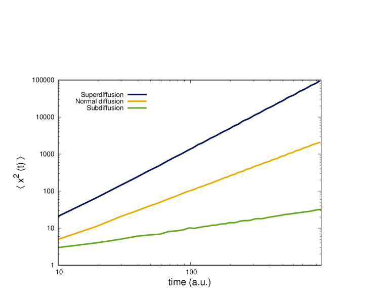
Figure 1: (Color ) Time evolution of the mean square displacement (in arbitrary units) for normal and anomalous diffusion. For the upper curve $\alpha=1.5$ (superdiffusion), for the middle curve $\alpha=1$ (normal diffusion) and for the lower curve $\alpha=0.5$ (subdiffusion). From ref. Lapas et al. (2008), with permission from Physical Review Letters.

The origin of this discrepancy is the tacit assumption made in the derivation of (1) that the Brownian particle moves in an infinite structureless medium acting as a heat bath. This assumption is generally incorrect when the Brownian motion takes place in a complex medium, as is the case of the previously mentioned examples. We illustrate in Fig. (1) the mean square displacement $\langle x^{2}(t)\rangle$ as a function of $t$ for three distinct Brownian motions in one dimension. From the upper curve downwards, we have $\alpha=1.5$ (superdiffusion), $\alpha=1$ (normal diffusion), and $\alpha=0.5$ (subdiffusion).

The recent interest in the study of complex systems has led to an increased focus on anomalous diffusion Metzler and Klafter (2000); Morgado et al. (2002); Metzler and Klafter (2004); Sancho et al. (2004); Yulmetyev et al. (2003); Santamaría-Holek et al. (2009); Durang et al. (2015), which has been described in biological systems Santamaría-Holek et al. (2009); Palmieri et al. (2015); Lomholt et al. (2005), protostellar birth Vaytet, N. et al. (2018), complex fluids Mason and Weitz (1995); Grmela and Öttinger (1997); Bakk et al. (2002); Sehnem et al. (2014, 2015); Cabreira Gomes et al. (2018), electronic transportation de Brito et al. (1995); Monte et al. (2000, 2002); Kumakura et al. (2005); Borges et al. (2006); Gudowska-Nowak et al. (2005), porous media and infiltration Filipovitch et al. (2016); Aarão Reis (2016); Aarão Reis et al. (2018), drug delivery Gomes Filho et al. (2016); Ignacio et al. (2017); Gun et al. (2017); Soares et al. (2017), fractal structures and networks Mandelbrot (1982); Stauffer and Stanley (1995); Cristea and Steinsky (2014); Balankin (2017, 2018), and in water’s anomalous behavior Barbosa et al. (2011); Bertolazzo et al. (2015); da Silva et al. (2015), phase transitions in synchronizing oscillators Cieśla et al. (2001); Longa et al. (1996); Bier et al. (2016); Pinto et al. (2016, 2017), to name a few.

There are many formalisms that describe anomalous diffusion, ranging from thermodynamics Pérez-Madrid (2004); Rubí and Bedeaux (1988); Kuśmierz et al. (2018), and fractional derivatives Metzler and Klafter (2000, 2004) to generalized Langevin equations (GLE) Hänggi et al. (1990); Morgado et al. (2007); Lapas et al. (2007). The goal of this short review is to call attention to relevant research within the GLE framework and to some fundamental theorems in statistical mechanics.

III The generalized Langevin equation approach

III.1 Non-Markovian processes

The Langevin formalism within its classical description has some restrictions:

1. It has a relaxation time $\tau=\gamma^{-1}$ , and an unspecified $\Delta t\ll\tau$, while a diffusive process in a real system can present several time scales;

2. For short times $t<\Delta t$, predictions are unrealistic; for example, the derivative of $C_{v}(t)$ is zero Lee (1983a) at $t=0$, while in Langevin’s formalism $C_{v}(t)=\exp(-\gamma|t|)$, exhibiting a discontinuity.

3. If no external field is applied it cannot predict anomalous diffusion.

Up to now we have used time and ensemble averages without distinction, i.e. we implicitly used the Boltzmann Ergodic hypothesis (EH). The ensemble average for a variable $B(t)$ is defined by

$$\langle B(t)\rangle=\int\exp{(-E/(k_{B}T))}\Omega(E,B)B(t)dE,$$ (19)

where $\Omega(E,B)$ is the number of states for a given energy $E$. For the time average we have

$$\overline{B(t)}=\frac{1}{\tau_{0}}\int_{-\tau_{0}/2}^{\tau_{0}/2}B(t+t^{\prime})dt^{\prime}.$$ (20)

For times $\tau_{0}\gg\tau$, the Ergodic Hypothesis (EH) reads

$$\overline{B(t)}=\langle B(t)\rangle,$$ (21)

which means that the system should be able to reach every accessible state in configuration space given enough time. This is expected to be true for equilibrated macroscopic systems and also for systems that suffer small perturbations close to equilibrium.

In this section, we generalize Langevin‘s equation and study some of its consequence for diffusion. The first correction to the FDT was done by Nyquist Nyquist (1928) who formulated a quantum version of the FDT. Later on Mori Mori (1965, 1965) and Kubo Kubo (1974) used a projection operator method to obtain the equation of motion, the Generalized Langevin equation (GLE),

$$\frac{dA(t)}{dt}=-\int_{0}^{t}\Pi(t-t^{\prime})A(t^{\prime})\,dt^{\prime}+F(t),$$ (22)

for a dynamical operator $A(t)$, where $\Pi(t)$ is a non-Markovian memory and $F(t)$ is a random variable subject to

1. $\overline{F(t)}=0$,

2. $\overline{F(t)A(0)}=0$, and,

3. the Kubo fluctuation-dissipation theorem (FDT) Kubo et al. (1991); Kubo (1966)

   $$C_{F}(t-t^{\prime})=\overline{F(t)F(t^{\prime})}=\langle A^{2}\rangle_{eq}\,\Pi(t-t^{\prime}).$$ (23)

In this way, it is clear that time translational invariance holds in the Kubo formalism. An alternative to the projection operators, the recurrence relation method, was derived by Lee Lee (1983a, 1982, b); Lee and Hong (1984).

It is easy to show that Equation (22) can give rise both to normal and to anomalous diffusion Vainstein et al. (2006a). Let us consider two limiting case examples: first, when $\Pi(t)=2\gamma\delta(t)$, we recover the normal Langevin equation (9) with normal diffusion ($\alpha=1$); second, for a constant memory $\Pi(t)=K$, Equation (22) becomes

$$\frac{d^{2}x}{dt^{2}}=-Kx+F(t),$$ (24)

where

$$x(t)=\int_{0}^{t}A(t^{\prime})\,dt^{\prime}.$$ (25)

Equation (24) is the equation of motion for a harmonic oscillator with zero diffusion constant ($D=0$) and with exponent $\alpha=0$. Consequently, we may have different classes of diffusion for distinct memories.

Now, we can study the asymptotic behavior of Equation (25) or of its second moment, Equation (18), to characterize the type of diffusion presented by the system for any memory $\Pi(t)$. Much information about the system’s relaxation properties can be obtained by studying the correlation function

$$C_{A}(t,t^{\prime})=\overline{A(t)A(t^{\prime})}=C_{A}(t-t^{\prime}).$$ (26)

The existence of stationary states warrants time-translation invariance so that the the two-time correlation function becomes a function only of the difference between two times, such as in the Kubo FDT above. We shall return to this point later. The main equation we are interested in is Equation (1), where for anomalous diffusion, $D$ should be replaced by $D(t)$ now defined by $D(t)=\int_{0}^{t}C_{A}(t^{\prime})dt^{\prime}$ then

$$\lim_{t\rightarrow\infty}D(t)=\lim_{t\rightarrow\infty}\int_{0}^{t}C_{A}(t^{\prime})dt^{\prime}=\lim_{z\rightarrow 0}\widetilde{C}_{A}(z).$$ (27)

From here onwards, the tilde over the function stands for the Laplace transform. For the last equality, we use the final-value theorem for Laplace transforms Gluskin (2003), which states that if $f(t)$ is bounded on $(0,\infty)$ and $\lim_{t\rightarrow\infty}f(t)$ has a finite limit, then $\lim_{t\rightarrow\infty}f(t)=\lim_{z\rightarrow 0}{z\widetilde{f}(z)}$. Also note that the Laplace transform of the integral of a function is the Laplace transform of the function divided by $z$, then $\widetilde{D}(z)=\widetilde{C}_{A}(z)/z$. Using $z\propto 1/t$, we obtain the asymptotic behavior of $D(t)$. In order to do that, we multiply Eq. ( 22) by $A(0)$, take the average and use the conditions $(1)$ and $(2)$ above for the noise to obtain the self-consistent equation

$$\frac{dR(t)}{dt}=-\int_{0}^{t}\Pi(t-t^{\prime})R(t^{\prime})\,dt^{\prime},$$ (28)

where for simplicity we have defined

$$R(t)=\frac{C_{A}(t)}{C_{A}(0)}.$$ (29)

Note that from Equation (22), we need to average from a large number of stochastic trajectories, while to obtain Eq.  (29), it is only necessary to solve a single equation, i.e. Eq. (28). Further insight can be gained by analyzing the Laplace transformed version of Equation (28)

$$\widetilde{R}(z)=\frac{1}{z+\widetilde{\Pi}(z)}.$$ (30)

From here, it is clear that the knowledge of $\widetilde{\Pi}(z)$ in the limit $z\to 0$ completely defines the asymptotic dynamics. For instance, if $\lim_{z\rightarrow 0}\widetilde{\Pi}(z)\propto z^{\mu}$ then Equation (27) becomes

$$\lim_{t\rightarrow\infty}D(t)\propto t^{\beta}$$ (31)

and consequently Morgado et al. (2002)

$$\alpha=\beta+1,$$ (32)

where

$$\beta=\begin{cases}\mu,&\text{ if~{}~{} }-1<\mu<1\\ 1,&\text{ if~{}~{} }\mu\geq 1,\\ \end{cases}$$ (33)

We see that we have a cutoff limit for the exponent $\beta$ and, therefore, also for $\alpha$.

Due to the existence of correlations in the GLE that arise through hydrodynamical interactions Reichl (1998), it has been proposed Morgado et al. (2002); Vainstein et al. (2005); Morgado et al. (2004) to establish a connection between the random force $F(t)$ and the noise density of states $\rho(\omega)$ of the surrounding media, modeled as a thermal bath of harmonic oscillators Morgado et al. (2002); Hänggi et al. (1990) of the form

$$F(t)=\int C(\omega)\cos[\omega t+\phi(\omega)]d\omega,$$ (34)

where $0<\phi<\pi$ are random phases. Now, using the Kubo FDT, eq. (23), and time averaging over the cosines, we obtain the memory as Morgado et al. (2002); Costa et al. (2003)

$$\Pi(t)=\int\rho(\omega)\cos(\omega t)d\omega,$$ (35)

which is an even function independent of the noise distribution. Here, $\rho(\omega)=C^{2}(\omega)\langle A^{2}\rangle_{eq}/2$.

The consequences of considering a colored noise given by a generalization of the Debye spectrum

$$\rho(\omega)=\begin{cases}\frac{2\gamma}{\pi}\left(\frac{\omega}{\omega_{s}}\right)^{\nu},&\text{ if }\omega<\omega_{s}\\ 0,&\text{ otherwise},\end{cases}$$ (36)

with $\omega_{s}$ as a Debye cutoff frequency were analyzed in detail in Vainstein et al. (2006b). The reason for the choice of this functional form for the noise density of states is that it was previously shown in Morgado et al. (2002); Costa et al. (2003) that if $\widetilde{\Pi}(z)\propto z^{\mu}$ as $z\rightarrow 0$, then the same restriction as in Equation (33), with $\nu=\mu$, applies and the diffusion exponent Morgado et al. (2002) is given by Equation (32).

Later, this problem was revisited by Ferreira et al. Ferreira et al. (2012) in which a generalized version of Equation (18) was considered, namely

$$\lim_{t\rightarrow\infty}\left\langle r^{2}(t)\right\rangle\sim t^{\alpha}(ln(t))^{\pm n}.$$ (37)

Most authors Metzler and Klafter (2000); Morgado et al. (2002); Metzler and Klafter (2004); Morgado et al. (2004) have reported the cases of anomalous diffusion where, $n=0$ and $\alpha\neq 1$. However, some authors such as for example, Srokowksi Srokowski (2000, 2013) reports situations were for $t\rightarrow\infty$, the dispersion behaves as

$$\langle x^{2}(t)\rangle\propto t/\ln(t),$$ (38)

i.e., a weak subdiffusive behavior for which we can say that $\alpha=1^{-}$. In this way Ferreira et al. Ferreira et al. (2012) generalizes the concept of $\alpha$, to associate with Eq. (37), the $\alpha^{\pm}$ exponents, which arise analogously to the critical exponents of a phase transition Kadanoff et al. (1967); Kadanoff (2000); Kenna et al. (2006). For example, in magnetic systems with temperatures $T$ close to the transition temperature $T_{c}$, the specific heat at zero field, $H=0$, exhibits the power law behavior $C_{H=0}\propto|T-T_{c}|^{-\alpha}$, where $\alpha$ is the critical exponent. However, for the two-dimensional Ising model Kadanoff et al. (1967) the critical exponent can be considered $\alpha=0^{+}$, since the specific heat behaves logarithmically, $C_{H=0}\propto\ln{|T-T_{c}|}$, instead. Logarithmic corrections Kenna et al. (2006) to scaling have also been applied to the diluted Ising model in two dimensions in Kenna and Ruiz-Lorenzo (2008). This generalized nomenclature is pertinent because there are many possible combinations of both logarithmic and power law behaviors. This result highlights the existence of different types of diffusion.

In this way, for the density of states (36), the generalized $\alpha$ becomes

$$\alpha=\begin{cases}2,&\text{ if~{}~{} }\nu>1\\ 2^{-},&\text{ if~{}~{} }\nu=1\\ 1+\nu,&\text{ if~{}~{} }-1<\nu<1.\end{cases}$$ (39)

In Equation (36), we choose the constant such that for normal diffusion $\widetilde{\Gamma}(z=0)=\gamma$. The exponent for Ballistic diffusion (BD), $\alpha=2$, is the maximum for diffusion in the absence of an external field. The slow ballistic motion $\alpha=2^{-}$ has properties that differ markedly from the ballistic case, see sections (3.3 and 3.4).

III.2 Non-exponential relaxation

Besides the importance of the asymptotic behavior, the study of the correlation $R(t)$ for finite times is also obviously significant, and there exists a vast literature describing non-exponential behavior of correlation functions in systems ranging from plasmas to hydrated proteins Rubí et al. (2004); Santamaría-Holek et al. (2004); Vainstein et al. (2003); Santos et al. (2000); Benmouna et al. (2001); Peyrard (2001); Colaiori and Moore (2001a); Ferreira et al. (1991); Bouchaud et al. (1991), since the pioneering works of Rudolph Kohlrausch Kohlrausch (1854) who described charge relaxation in Leyden jars using stretched exponentials, $R(t)\approx\exp{[-(t/\tau)^{\beta}]}$ with $0<\beta<1$, and his son Friedrich Kohlrausch Kohlrausch (1863), who observed two universal behaviors: the stretched exponential and the power law. Since many features are shared among such systems and those that present anomalous diffusion Vainstein et al. (2005); Lapas et al. (2015), it is natural that similar methods of analysis can be applied to both. For example, from Equation (28), $\frac{dR(t)}{dt}$ must be zero at $t=0$, which is at odds with the result $R(t)=\exp(-\gamma|t|)$ of the memoryless Langevin equation. Nevertheless, we know that the exponential can be a reasonable approximation in some cases: Vainstein et al. Vainstein et al. (2006b) have presented a large diversity of correlation functions that can be obtained from Equation (28) once $\Pi(t)$ is known. Since, from Equation (35), $\Pi(t)$ is an even function then we can write

$$\Pi(t)=\sum_{n=0}^{\infty}b_{n}t^{2n}.$$ (40)

From Equation (28), they proved that $R(t)$ must also be an even function, therefore

$$R(t)=\sum_{n=0}^{\infty}a_{n}t^{2n},$$ (41)

with $a_{0}=R(0)=1$. We insert Equations (40) and (41) into Equation (28) to obtain the recurrence relation Vainstein et al. (2006b)

$$a_{n}=-\frac{2\gamma\omega_{s}}{\pi(2n)!}\sum_{l=0}^{n-1}\frac{(-1)^{l}[2(n-1-l)]!\,\omega_{s}^{2l}}{(2l+1+\nu)}a_{n-1-l},$$ (42)

which shows the richness and complexity of behavior that can arise from a non-Markovian model. The above defined convergent power series represents a large class of functions, including the Mittag-Leffler function Mittag-Leffler (1905) which behaves as a stretched exponential for short times and as an inverse power law in the long time scale. Note that even for the simplest case of normal diffusion, $\nu=0$, $R(t)$ is not an exponential since at the origin its derivative is zero; however, for broad-band noise $\omega_{s}\gg\gamma$, i.e., in the limit of white noise it approaches the exponential $R(t)=\exp(-\gamma t)$, for times larger than $\tau_{s}=\omega_{s}^{-1}$.

Figure 2: Plot of the correlation function $R(t)$ for normal diffusion ($\nu=0$). Here, $\gamma=1$ and $\omega_{s}=2$ and $20$, for curves $a$ and $b$, respectively. Curve $c$ is the plot of $\exp(-\gamma t)$. Note that curves $b$ and $c$ are indistinguishable, except near the origin (see inset). Inset: Plot of curves $b$, $c$ and $\cos(\omega_{0}t)$, near the origin. From ref. Vainstein et al. (2006a), with permission from Europhysics Letters.

In Fig. (2), from Vainstein et al. (2006b), we display the rich behavior of the correlation function $R(t)$ for the case of normal diffusion. Here, $\gamma=1$ and $\omega_{s}=2$ and $20$, for curves $a$ and $b$, respectively. Curve $c$ is the plot of $\exp(-\gamma t)$. In the inset, we highlight that although curve $b$ and the exponential approach one another for long times, for short times they differ appreciably. Also plotted is $\cos(\omega_{0}t)$, with $\omega_{0}=\sqrt{\Pi(0)}$.

III.3 Basic theorems of statistical mechanics

III.3.1 The decay towards an equilibrium state

One of the most important aspects of dynamics is to observe the asymptotic behavior of a system or how it approaches equilibrium (or not). Observe that a direct solution for Equation (22) is

$$A(t)=A(0)R(t)+\int_{0}^{t}R\left(t-t^{\prime}\right)F(t)dt.$$ (43)

Given the initial states $A(0)$, it is possible to average over many trajectories to obtain the temporal evolution of the moments $\overline{A^{n}(t)}$, with $n=1,2,\ldots$. The first moment arises directly from an average of Equation (43),

$$\overline{A(t)}=\overline{A(0)}R(t)\text{.}$$ (44)

Taking the square of Equation (43) and averaging, we obtain

$$\overline{A^{2}}=\overline{A^{2}}+R^{2}(t)\left[\overline{A^{2}(0)}-\langle A^{2}\rangle_{eq}\right]\text{.}$$ (45)

The skewness is defined as a measure of the degree of asymmetry of the distribution of $A(t)$, and is given by Lapas et al. (2007)

$$\zeta(t)=\left[\frac{\sigma_{A}(0)}{\sigma_{A}(t)}\right]\zeta(0)R^{3}(t),$$ (46)

where $\sigma_{A}(t)=\overline{A^{2}(t)}-\overline{A(t)}^{2}$. We also obtain the non-Gaussian factor Lapas et al. (2007)

$$\eta(t)=\left[\frac{\overline{A^{2}(0)}}{\overline{A^{2}(t)}}\right]\eta(0)R^{4}(t).$$ (47)

Consequently, we see that $R(t)$ completely determines these averages. One can note that if the system is originally at equilibrium $\overline{A(0)}=0$ and $\overline{A^{2}(0)}=\left\langle A^{2}\right\rangle_{eq}$, then the system remains in equilibrium. If the system is not in equilibrium, then

$$\lim_{t\rightarrow\infty}R(t)=0$$ (48)

drives the system towards equilibrium. The condition stated in Equation (48) is called the mixing condition (MC) and is a fundamental concept in statistical mechanics, which asserts that after a long time the system reaches equilibrium and forgets all initial conditions.

Note that parity is conserved as well: if the initial skewness is null, $\zeta(0)=0$ in Eq. (46), it will remain null during the whole evolution; the same holds for the nongaussian factor.

III.3.2 The Kinchin theorem and ergodicity

The Khinchin theorem (KT) Lapas et al. (2008); Khinchin (1949) states that if the the MC holds, then ergodicity holds. As shown below, anomalous diffusion is a good field for testing ergodicity breaking Lapas et al. (2008); Weron and Magdziarz (2010); Lapas et al. (2007). For a situation where the MC is violated, we have

$$\kappa=\lim_{t\rightarrow\infty}R(t)=\lim_{z\rightarrow 0}z\widetilde{R}(z)=\lim_{z\rightarrow 0}\left[1+\frac{\widetilde{\Pi}(z)}{z}\right]^{-1}\neq 0,$$ (49)

where $\kappa$ is the nonergodic factor Costa et al. (2003); Lapas et al. (2008); Bao et al. (2006, 2005). For example for $\widetilde{\Pi}(z\rightarrow 0)\propto bz$ , $\alpha=2$, and

$$\kappa=\frac{1}{1+b}.$$ (50)

I.e., the MC is violated in the ballistic motion, and consequently ergodicity is violated, but not the KT. Note that for $\alpha=2^{-}$, where $R(t\rightarrow\infty)\rightarrow 1/\ln(t)\rightarrow 0$, the MC is not violated. In this way the MC is satisfied for all diffusive processes in the range $0<\alpha<2^{-}$ Ferreira et al. (2012).

It is interesting to observe that Equation (49) for long time behavior is equivalent to the condition

$$\Lambda=\int U(\vec{r})\,d\vec{r}\to\infty,$$ (51)

for systems with long range interactions Silvestre and Rocha Filho (2016); Campa et al. (2009), where $U(\vec{r})$ is the potential between the particles and the integration is performed over all space.

III.3.3 Gaussianization

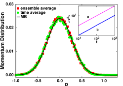
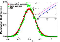
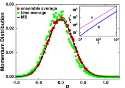
Figure 3: (Color online) Numerical results for the probability distribution function for subdiffusion (left, $\alpha=0.5$), normal diffusion (middle, $\alpha=1$) and superdiffusion (right, $\alpha=1.5$). The time averages (circles) are obtained by following one particle trajectory and calculating the histogram for times from $t=100$ to $t=5000$. For the ensemble averages (squares), we calculate the histogram using $5\cdot 10^{4}$ particles, at time $t=1000$. The continuous line is the Maxwell-Boltzmann distribution. Insets: Curves $a$ correspond to the functions $t^{\alpha}$ and curves $b$ to the simulated mean square displacements. From Lapas et al. Lapas et al. (2008), with permission from Physical Review Letters.

As an illustration of the analytical results, we numerically integrated the GLE, Equation (22), to approximate the particle velocity distribution function, using Equations (35) and (36) to generate the memory for $\nu=-0.5$, $0$, and $0.5$, which by Equation (39) give $\alpha=0.5$, $1$, and $1.5$, respectively. The results are exhibited in Fig. (3), from  Lapas et al. (2008), where we show the probability distribution functions as function of the momentum $p$. From left to right, we have subdiffusion ($\nu=-0.5$), normal diffusion ($\nu=0$), and superdiffusion ($\nu=0.5$) for the values $a=\frac{2\gamma}{\pi}=0.25$. A value $\omega_{s}=0.5$ was used for normal and superdiffusion. In the case of subdiffusion, a broader noise $\omega_{s}=2$ is needed for it to arrive at the stationary state. It is expected that $R(t\rightarrow\infty)=0$ in all cases, and that the EH will be valid even for the subdiffusion (superdiffusion). It should be noted that despite large fluctuations in the time average, there is a good agreement between the ensemble and time distributions, in agreement with Eqs. (44) to (48), indicating the validity of the EH. In all cases, the distributions converge to the expected Maxwell-Boltzmann distribution, in accordance with analytical results Lapas et al. (2007).

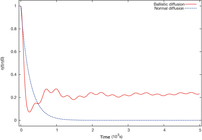
Figure 4: (Color online) Time evolution of the normalized non-Gaussian factor $\eta(t)/\eta(0)$ for normal and ballistic diffusion. In both cases, we consider the initial PDF as a Laplace distribution with unit mean and unit variance. The functions $R(t)$ are as in Fig. (5). From Lapas et al. (2007), with permission from Europhysics Letters.

In Fig. (4 we show the evolution of the nongaussian factor. We see that for the Ballistic diffusion (BD), it does not reach a null value, but it evolves towards it. Note that even for a situation where $\kappa\neq 0$, the nongaussian factor will be very small and the probability of it being non-zero in simulations after a long time is very small. For example for $\kappa=0.1$, there will a factor of $10^{-4}$ in relation (47).

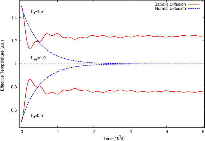
Figure 5: (Color ) Time evolution of the effective kinetic temperature (in arbitrary units) for normal and ballistic diffusion. For BD we use the noise distribution $\rho(\omega)=2\gamma/\pi$ for $1<\omega<4$ and $\rho(\omega)=0$, otherwise, and we found $R(t)$ numerically (solid curve). Since BD converges very slowly, we use $\gamma=1$ for BD and $\gamma=10^{-3}$ for normal diffusion with $R(t)=\exp(-\gamma t)$, so we can compare both. We choose $T_{0}=1.5$ and $T_{0}=0.5$ for the initial temperatures. In both cases we used $T=1$ for the reservoir temperature. From Lapas et al. (2007), with permission from Europhysics Letters.

In Fig. (5), from Lapas et al. (2007), we show the evolution of the kinetic temperature of the system by taking $A^{2}(t)$, with $A=P$, the momentum of the particles. In this case we should have $\langle A^{2}\rangle_{eq}-\langle A\rangle^{2}_{eq}\propto T$ Lapas et al. (2007) and the temperature evolution can be obtained from Equation (45). We consider both normal and ballistic diffusion (BD) in a reservoir characterized by $T=1.0$ with initial high and low temperatures $T_{0}=1.5$ and $T_{0}=0.5$, respectively. For normal diffusion (dashed curve), we have $R(t)=\exp{(-\gamma t)}$, with $\gamma=10^{-3}$. For BD, $R(t)$ is calculated numerically in Lapas et al. (2007) with $\gamma=1$. Since BD’s relaxation is slow, we take a “friction” $\gamma$ a thousand times larger than that of normal diffusion for comparison. As expected, in the case of normal diffusion the system’s temperature always relaxes to that of the reservoir, while for BD the temperature approaches that of the reservoir without reaching it Lapas et al. (2007, 2015). Figure (4) displays the normalized non-Gaussian factor, Equation (47), as a function of time Lapas et al. (2007) for the cases in the previous figure, with the same convention for the labeling. For normal diffusion, the system’s probability distribution evolves towards a Gaussian, which is not the case for BD. In the latter case, $R(t)$ oscillates around the value predicted by Equation (50), even for long times, In both cases, the initial probability distribution function was the Laplace distribution, with $\langle A^{2}(0)\rangle=1$ and $\langle A(0)\rangle=0$.

III.3.4 The fluctuation-dissipation theorem

Figures (3)–(4) are just illustrations of the results that can be obtained analytically from Equations (48) to (21). Lapas et al. Lapas et al. (2008, 2007) have shown that the KT is valid for all forms of diffusion, and that the ballistic diffusion violates the EH, but not the KT.

Although it is expected that a system in contact with a heat reservoir will be driven to equilibrium by fluctuations, Figs.(5) and (4) show that it is not always the case and in some far from equilibrium situation it may not happen. The concept of “far from equilibrium” is itself sometimes misleading, since it depends not only on the initial conditions, but also on the possible trajectories the system may follow Costa et al. (2003); Rubí et al. (2004); Santamaría-Holek et al. (2004). It was a known fact that the FDT can be violated in many slow relaxation processes Parisi (1997); Vainstein et al. (2006a); Dybiec et al. (2012), however, it was a surprise that it could occur in a GLE without disorder Cugliandolo et al. (1994) or an external field Costa et al. (2003); Dyre and Schrøder (2000); Vainstein et al. (2006a). Finally, Costa et al. Costa et al. (2003) have called attention to the fact that if after a long time the fluctuations are not enough to drive the system to equilibrium then the fluctuation-dissipation theorem is violated. For the dissipation relation to be fulfilled, the MC condition, Equation (48), must be valid.

IV Beyond the basics… and more basic

In the last sections we have discussed some basic results for anomalous diffusion under the point of view of the formalism of the generalized Langevin equation which yield two main features: simplicity and exact results. Obviously, this approach does not exhaust the subject, since diffusion is a basic phenomenon in physics it is a starting point to many different formalisms which we shall briefly discuss.

IV.1 Fractional Fokker-Planck equation

We have seen that, in principle, all kinds of anomalous diffusion can be described by the GLE formalism, which is itself well established from the Mori method. Since normal diffusion can be studied both from Langevin equations and from Fokker-Planck equations, we would expect to obtain a generalized Fokker-Planck formalism for anomalous diffusion. Indeed, fractal formulations of the Fokker-Planck equation (FFPE) have been widely used in the literature in the last decades, in which the evolution of the probability distribution function $P(x,t)$ reads Metzler et al. (1999); Metzler and Klafter (2000, 2004)

$$\frac{\partial^{\alpha}P(x,t)}{\partial t^{\alpha}}=\left[\frac{1}{m\gamma_{\alpha}}\frac{\partial U(x)}{\partial x}+D_{\alpha}\frac{\partial^{2}}{\partial x^{2}}\right]P(x,t),$$ (52)

where on the left-hand-side a fractional Rieman-Liouville time-derivative is defined as Oldham and Spanier (1974)

$$\frac{\partial^{\alpha}P(x,t)}{\partial t^{\alpha}}=\frac{1}{\Gamma(1-\alpha)}\frac{\partial}{\partial t}\int_{0}^{t}\frac{P(x,s)}{(t-s)^{\alpha}}ds,$$ (53)

with $0<\alpha<1$. Note that the definition of fractional derivatives is not unique Oldham and Spanier (1974); Kilbas et al. (2006), with a variety of possibilities, physically (almost) totally unexplored. We notice here that the nonlocal character of the fractional Fokker-Planck equation is similar to the memory kernel in the GLE. On the right hand side, $\gamma_{\alpha}$ is a generalized friction, $U(x)$ is the potential, while $D_{\alpha}$ is generalized Einstein-Stokes relation

$$D_{\alpha}=\frac{k_{B}T}{m\gamma_{\alpha}}.$$ (54)

The major result from Equation (52) for a force-free diffusion is the asymptotic solution

$$\lim_{t\rightarrow\infty}\langle x^{2}(t)\rangle=\frac{2D_{\alpha}}{\Gamma(1+\alpha)}t^{\alpha}.$$ (55)

Again, for $\alpha\neq 1$, we reach an anomalous diffusion regime Shlesinger et al. (1993); Metzler and Klafter (2000, 2004); Klafter et al. (1996).

IV.2 Interface growth

Models for interface growth generally consider the random deposition of particles that diffuse to a surface and, as such, have been studied with Langevin equations and modified diffusion equations. Since diffusion with subsequent deposition is ubiquitous, rough surfaces at the interface of two media are very common in nature  Barabási and Stanley (1995); Edwards and Wilkinson (1982); Kardar et al. (1986); Hansen et al. (2000); Cordeiro et al. (2001); Schmittbuhl et al. (2006) and the description of interface evolution is a very interesting problem in statistical physics. The major objective here is to describe the temporal evolution of the height $h(\vec{x},t)$ of the interface between two substrates Barabási and Stanley (1995); Edwards and Wilkinson (1982), where $\vec{x}$ is the $d$ dimensional position vector and $t$ is the time. We outline the evolution of $h$ in Fig. (6). In (a), we show a real forest fire propagation, a very complex situation. However, we can focus on the interface between the burnt and unburned regions. In (b), we provide a snapshot at a fixed time $t$ of the height $h(\vec{x},t)$ for a microscopic growth process in which the green medium is penetrating the blue one with arbitrary units. These types of dynamics in $d+1$ dimensional space are easy to understand, but not so simple to solve analytically. Experiments can be done for $d=1,2,3$; however, they present hard theoretical problems for any $d$.

The two main quantities of interest are the average height

$$\langle h(t)\rangle=\frac{1}{V}\int h(\vec{x},t)d\vec{x},$$ (56)

where $V$ is the sample volume, and the standard deviation

$$w^{2}(t)=\langle h^{2}(t)\rangle-\langle h(t)\rangle^{2},$$ (57)

often called the surface width $w(t)$, or roughness. Not surprisingly, this height fluctuation has a lot of information about the physical processes governing the system. The evolution of $w(t)$ observed through experiments, computer simulations, and a few analytical results gives us some general features of growth dynamics.

Starting with a flat surface, $w(0)=0$, the evolution exhibits four distinct regions: (a) for a very short period $0<t<t_{0}$, during which correlations are negligible, the process is a random deposition $w(t)\sim t^{1/2}$; (b) for $t_{0}<t<t_{\times}$ we have $w(t)\sim t^{\beta}$. Here the $t_{\times}$ follows a power law of the form $t_{\times}\sim L^{z}$, where $L$ is the size of the sample, $z$ is the dynamic exponent, and $\beta$ the growth exponent; (c) there is a transition region for $t\sim t_{\times}$; (d) finally, for $t\gg t_{\times}$, the dynamic equilibrium leads to surface width saturation, $w_{s}$, which also follows a power law $w_{s}\sim L^{\alpha}$, where $\alpha$ is the roughness exponent. The crossing of the curves $w(t)\sim t^{\beta}$ and $w\sim w_{s}$ yields the universal relation

$$z=\frac{\alpha}{\beta}.$$ (58)

It should be pointed out that these exponents are not related with those of the previous section.

To obtain $w(t)$, we need to know $h(\vec{x},t)$ and there are two major theoretical ways to attack this problem: 1. Continuous growth equations; 2. Discrete growth models. Fig. (6a) is an example of the first, while Fig. (6b) is an example of the second.

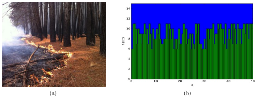
Figure 6: (Color online) (a) Fire propagation in the Amazon rainforest. Source: http://g1.globo.com/am/amazonas/noticia/2013/01/florestas-no-sul-do-am-estao-mais-vulneraveis-incendio-aponta-estudo.html; (b) Schematic representation on a microscopic scale of the height evolution $h(\vec{x},t)$, defining the interface between two media, as function of the position $\vec{x}$ for a given time $t$.

IV.2.1 Equation of motion and symmetries

The growth, in general, is due to the number of particles per unit of time $G(\vec{x},t)$ arriving on the surface at the position $\vec{x}$ and time $t$. The particle flux is not uniform since the particles are deposited at random positions Barabási and Stanley (1995). Therefore, the evolution of $h(\vec{x},t)$ can be described by

$$\frac{\partial h(\vec{x},t)}{\partial t}=G=F+\chi(\vec{x},t),$$ (59)

where the first term $F$ is the average number of particles arriving at site $\vec{x}$. The second term, $\chi(\vec{x},t)$, reflects the random fluctuations and satisfies

$$\langle\chi({\vec{x},t})\rangle=0,\text{ and }$$ (60)

$$\langle\chi({\vec{x},t})\chi({\vec{x}\,^{\prime},t^{\prime}})\rangle=2D_{g}\delta(\vec{x}-\vec{x}\,^{\prime})\delta(t-t^{\prime}),$$ (61)

where, $D_{g}$ measures the degree of growth randomness. The deterministic flux $F$ must satisfy certain symmetry requirements, such as invariance under translation of position, $\vec{x}\rightarrow\vec{x}+\vec{x_{0}}$, height, $h\rightarrow h+h_{0}$ and time $t\rightarrow t+t_{0}$. To satisfy these conditions, it must depend only on derivatives, which, again by the symmetries $\vec{x}\rightarrow-\vec{x}$ and $h\rightarrow-h$, must be of even order Barabási and Stanley (1995); Edwards and Wilkinson (1982). Besides this, considering that symmetrically possible terms such as $\nabla^{2n}h(\vec{x},t)$, for $n=2,3,\dotsc$, are irrelevant in the long wavelength limit, since they go to zero faster than $\nabla^{2}h(\vec{x},t)$, we obtain, at the lowest-order in the derivatives Edwards and Wilkinson (1982),

$$\frac{\partial h(\vec{x},t)}{\partial t}=\nu\nabla^{2}h(\vec{x},t)+\chi(\vec{x},t),$$ (62)

known as Edwards-Wilkinson equation (EW). Note that it is basically a diffusion equation, as (2), plus a noise, where we have a surface tension $\nu$ associated with the Laplacian smoothening mechanism. The random deposition model with surface relaxation is in the same universality class as the EW model Horowitz et al. (2001), i.e., they share the same exponents.

Because there are, however, a large class of growth phenomena which are not described by the EW equation, new formulations become necessary. The recently proposed Arcetri models Henkel and Durang (2015) allow the study of more rigid interfaces than the EW model and still allow for exact solutions in any dimension $d$. Depending on the initial conditions, both growing interfaces and particle motion on the lattice can be modeled. Another classical model was proposed by Kardar et al. Kardar et al. (1986), inspired by the stochastic Burgers equation. They observed that lateral growth could be added to this equation via the nonlinear term of the Burgers equation so that Equation (62) becomes

$$\dfrac{\partial h(\vec{x},t)}{\partial t}=\nu\nabla^{2}h(\vec{x},t)+\dfrac{\lambda}{2}[\vec{\nabla}h(\vec{x},t)]^{2}+\chi(\vec{x},t).$$ (63)

Since its formulation, the Kardar-Parisi-Zhang equation (KPZ) has been a prime model in the description of growth dynamics. The nonlinear term includes a new constant $\lambda$ associated with the tilt mechanism and breaks down the symmetry $h\rightarrow-h$. Consequently, the universality class of KPZ is different from that of EW.

Equation (63) is the simplest nonlinear equation that can describe a large number of growth processes Barabási and Stanley (1995); Kardar et al. (1986). However, the apparent simplicity of this equation is misleading, since the nonlinear gradient term combined with the noise makes it one of the toughest problems in modern mathematical physics Hairer (2013); Sasamoto and Spohn (2010). On the other hand, its complexity is compensated for its generality. It is connected to a large number of stochastic processes, such as the direct polymer model Kardar (1985), the weakly asymmetric simple exclusion process Bertini and Giacomin (1997), the totally asymmetric exclusion process Spitzer (1970), direct d-mer diffusion Ódor et al. (2010), fire propagation Myllys et al. (2001, 2003); Merikoski et al. (2003), atomic deposition Csahók and Vicsek (1992), evolution of bacterial colonies Ben-Jacob et al. (1994); Matsushita and Fujikawa (1990), turbulent liquid-crystals Takeuchi et al. (2011); Takeuchi and Sano (2012); Takeuchi (2013), polymer deposition in semiconductorsAlmeida et al. (2017), and etching Mello et al. (2001); Aarão Reis (2003, 2004, 2005); Oliveira and Aarão Reis (2008); Tang et al. (2010); Xun et al. (2012); Rodrigues et al. (2015); Mello (2015); Alves et al. (2016); Carrasco and Oliveira (2016, 2018).

This problem in non-equilibrium statistical physics is analogous to the Ising model for equilibrium statistical physics, which is used as a basic model for understanding a large class of phenomena. The search for exact solutions to this equation in the $d+1$ dimensional space has resulted in important contributions to mathematics; however, to date, they have been obtained only for specific situations and are limited to $1+1$ dimensions Kardar et al. (1986); Sasamoto and Spohn (2010) .

IV.2.2 Scaling invariance

In this small subsection we limit ourselves to scaling symmetries only. However, in interface growth, the shape of single-time and two-time responses and height correlation functions can be derived from the assumption of a local time-dependent scale-invariance Henkel (2017). For the KPZ equation, a systematic test of aging scaling was performed, showing the scaling relations for the two-time spatio-temporal autocorrelator and for the time-integrated response function Aarão Reis (2004); Henkel et al. (2012); Kelling et al. (2017a).

The scaling invariance can be investigated through the transformation Barabási and Stanley (1995) $\vec{x}\rightarrow b\vec{x}$, $h\rightarrow b^{\alpha}$ and $t\rightarrow t^{z}$ which yields, for the KPZ equation, (63),

$$\nu\rightarrow b^{z-2}\nu,$$ (64)

$$D_{g}\rightarrow b^{z-d-2\alpha}D_{g},$$ (65)

and

$$\lambda\rightarrow b^{\alpha+z-2}\lambda$$ (66)

Scaling invariance demands that the exponents in Equations (64,65, 66) must be zero. However, a simple inspection shows that they are inconsistent. The renormalization group approach of Kardar el al. Kardar et al. (1986), uses the nonlinear term as a perturbation, and their result shows that only Equation (66) remains invariant, yielding the famous Galilean invariance

$$\alpha+z=2.$$ (67)

Equations (64) and (65) are corrected by the renormalization, and the final result yields $\alpha=1/2$, $\beta=1/3$, and $z=3/2$, for $1+1$ dimensions. Since the KPZ renormalization approach is valid only for $1+1$ dimensions, questions about the validity of the Galilean invariance Wio et al. (2010, 2017) for $d>1$ and the existence of an upper critical dimension for KPZ Colaiori and Moore (2001b); Schwartz and Perlsman (2012) have been raised.

For $d>1$, the numerical simulation of the KPZ equation is not an easy task Wio et al. (2010, 2017); Lam and Shin (1998); Xu et al. (2006); Halpin-Healy and Takeuchi (2015); Torres and Buceta (2018), and the use of cellular automata models Mello et al. (2001); Aarão Reis (2003, 2004, 2005); Oliveira and Aarão Reis (2008); Tang et al. (2010); Xun et al. (2012); Rodrigues et al. (2015); Mello (2015); Alves et al. (2016); Carrasco and Oliveira (2016, 2018); Kelling et al. (2017b); Předota and Kotrla (1996); Chua et al. (2005); Buceta et al. (2014) has become increasingly common for growth simulations. Polynuclear growth (PNG), is a typical example of a discrete model that has received a lot of attention, and the outstanding works of Prähofer and Spohn Prähofer and Spohn (2000) and Johansson Johansson (2000) drive the way to the exact solution of the distributions of the heights fluctuations $f(h,t)$ in the KPZ equation for $1+1$ dimensions (Sasamoto and Spohn, 2010). By construction, $h\rightarrow h-\langle h\rangle$, then $f(h,t)$ has zero mean, so its skewness and kurtosis are the most important quantities to observe (Takeuchi, 2013; Oliveira et al., 2013; Alves et al., 2013; Almeida et al., 2014; Halpin-Healy and Zhang, 1995). In addition, Langevin equations for growth models have been discussed by some authors Haselwandter and Vvedensky (2006, 2008); Silveira and Aarão Reis (2012). Several works have been done in the weakly asymmetric simple exclusion process Bertini and Giacomin (1997), the totally asymmetric exclusion process Spitzer (1970); Alcaraz and Bariev (1999), and the direct d-mer diffusion model Ódor et al. (2010): for a review see (Halpin-Healy and Takeuchi, 2015; Halpin-Healy and Zhang, 1995; Meakin, 1993; Krug, 1997). More experimentally measured exponents for growing interfaces in four universality classes (KPZ, quenched KPZ, EW and Arcetri) can be found in Henkel and Durang (2015) and references therein.

IV.2.3 Cellular automata growth models

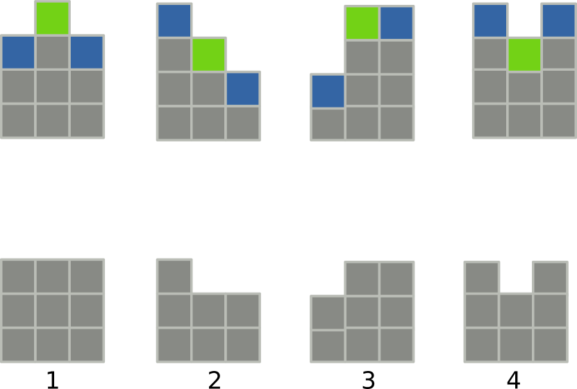
Figure 7: The etching mechanism in one dimension. The figures are the four situations in which the dynamics of the etching model can be divided. The initial configuration is at the top, where the selected site, in column 2, is green, and its first neighbors, in columns 1 and 3, are shown in dark blue. After the corrosion process the final situation is exhibited at the bottom. The steps are: step 1, site selection, green; step 2, interaction with nearest neighbors; step 3, decrease of height by one. From Alves et al. (2016), with permission from Physics Review E.

Cellular automata are described by simple rules, which allow us to inquire about relevant properties of a complex dynamical system. For a given growth model, the first question to be answered is if the model belongs to the same universality class as KPZ. In this context, we expose here the etching model Mello et al. (2001), which has attracted considerable attention in recent years Aarão Reis (2003, 2004, 2005); Oliveira and Aarão Reis (2008); Tang et al. (2010); Xun et al. (2012); Rodrigues et al. (2015); Mello (2015); Alves et al. (2016); Carrasco and Oliveira (2016, 2018). These studies suggest a close relation between the etching model and KPZ. For example, for $1+1$ dimensions Alves et al. Alves et al. (2016) have proven that $\alpha=1/2$ exactly. Unfortunately, their method does not allow to obtain $\beta$ or $z$.

The etching model describes the mechanism of an acid eroding a surface. The detailed description of the model can be found in Mello et al. (2001)) For simplicity, let us consider a site $i$ in a hypercube of side $L$ and volume $V=L^{d}$ in space $\Psi$ of dimension $d$, and look at one of its nearest neighbors, $j$. If $h_{j}>h_{i}$, then it becomes equal to $h_{i}$. We then define the etching model following the steps:

1. At time t we randomly choose a site $i\in{V}$.

2. If $h_{j}(t)>h_{i}(t)$, do $h_{j}(t+\Delta t)=h_{i}(t)$.

3. Do $h_{i}(t+\Delta t)=h_{i}(t)-1.$

In Fig. (7), we show the mechanism of the etching model in one dimension: (a) step 1, we randomly select a site at time $t$, here $i=2$ shown as green in the figure; step 2, the site $i=2$ interacts with its neighbors $j=1,3$. Then in Fig. (72) $h_{1}(t+\Delta t)=h_{2}(t)$, meaning that it is strongly affected, and $h_{3}(t+\Delta t)=h_{3}(t)$, meaning it is not affected; (c) step 3, $h_{2}(t+\Delta t)=h_{2}(t)-1$. We describe here a process of strong interactions between the site and its neighbors.

Using these rules and averaging over $N_{e}$ numerical experiments, it is possible to obtain the exponents $\alpha$, $\beta$, and $z$ Mello et al. (2001); Aarão Reis (2003, 2004, 2005); Oliveira and Aarão Reis (2008); Tang et al. (2010); Xun et al. (2012); Rodrigues et al. (2015); Mello (2015); Alves et al. (2016); Carrasco and Oliveira (2016, 2018). Finally, the upper critical limit for the etching model (KPZ) was recently discussed by Rodrigues et al. Rodrigues et al. (2015), where it was shown numerically that there is no upper critical dimension for the etching model up to $6+1$ dimensions. Thus, we have established a lower limit for the KPZ critical dimension, i.e., if it exists then $d_{c}>6$, in agreement with other authors Ódor et al. (2010). They have shown that the Galilean invariance (67) remains valid for $d\leq 6$ as well. These problems, however, still lack an exact solution.

IV.3 Reaction-diffusion processes

One could not complete a work on diffusion without a brief discussion of reaction-diffusion processes Alcaraz and Bariev (1999); Ben-Avraham and Havlin (2000); Abad et al. (2002); Shapoval et al. (2018). Exactly solvable reaction-diffusion models consist largely of single species reactions in one dimension, e.g., variations of the coalescence process, $A+A\rightarrow A+S$ Doering and Ben-Avraham (1989); Krebs et al. (1995); Simon (1995) and the annihilation process $A+A\rightarrow S+S$ Krebs et al. (1995); Simon (1995), where $A$ and $S$ denote occupied and empty sites, respectively. These simple reactions display a wide range of behavior characteristic of non-equilibrium kinetics, such as self organization, pattern formation, and kinetic phase transitions. Interval methods have provided many exact solutions for one-dimensional coalescence and annihilation models. The method of empty intervals, applicable to coalescence models, requires solution of an infinite hierarchy of differential difference equations for the probabilities $E_{n}$ of finding $n$ consecutive lattice sites simultaneously empty. For annihilation models, the method of parity intervals similarly requires determination of $G_{n}$, the probability of $n$ consecutive lattice sites containing an even number of particles Abad et al. (2002). In the continuous limit, such models can be described exactly in terms of the probability $E(t,x)$ of finding an empty interval of size $x$ at time $t$. Under fairly weak conditions, the equation of motion for $E(t,x)$ is a diffusion equation, albeit with the unusual boundary condition $E(t,0)=1$. In several cases, the exact and fluctuation-dominated behaviour in $d=1$ has been seen experimentally, since the 1990s. This is one of the rare cases where theoretical statistical mechanics can be compared with experiments and also shows that simple mean-field schemes are not enough. For an introduction see Ben-Avraham and Havlin (2000), and for up to date references see Shapoval et al. (2018).

Another important new development in diffusion concerns stochastic resets, as they were introduced by Evans and S.N. Majumdar (see Evans and Majumdar (2011, 2014); Durang et al. (2014) and references therein). This leads to important modifications of the stationary state and raises the question how to consider the status of the general theorem described in the present review.

V Conclusions

In this short review we address diffusion, as a modern and important topic of statistical physics, with broad applications Metzler and Klafter (2000); Morgado et al. (2002); Metzler and Klafter (2004); Costa et al. (2003); Lapas et al. (2008); Cieśla et al. (2001); Santamaría-Holek et al. (2009). We emphasize the study of systems with memory, for which a generalized Langevin equation applies and describe how the diffusion exponent is obtained from the memory Morgado et al. (2002); Ferreira et al. (2012). We highlight the properties of response functions Lapas et al. (2007); Vainstein et al. (2006a) for the processes of anomalous relaxation Vainstein et al. (2006a); Lapas et al. (2015), Gaussianization and ergodicity Lapas et al. (2008, 2007). Moreover, we have established a hierarchy: the mixing condition is stronger than the ergodic hypothesis, which is itself stronger than the fluctuation-dissipation theorem. It is important to call attention again to Costa Costa et al. (2003), where it was observed that in the ballistic diffusion the fluctuation-dissipation theorem fails. Indeed, for the ballistic motion which, on average, behaves as a Newtonian particle with constant velocity, the fluctuations are not enough to bring the system to equilibrium, i.e., the dissipation, which for large times decays as $1/t$, does not balance the fluctuations. This work points out that the violation of the mixing condition breaks down ergodicity, as required by the Khinchin theorem and the fluctuation dissipation theorem.

In conclusion, since the mechanism of diffusion is present in most nonequilibrium processes, diffusion is an exhaustive subject, and we have only called attention to some of its aspects. Consequently, we apologize to the authors of important works not mentioned here , such as aging Cugliandolo et al. (1994); Aarão Reis (2004); Henkel et al. (2012); Kelling et al. (2017a); Hodge (1995) for example.

Conflict of Interest Statement

The authors declare that the research was conducted in the absence of any commercial or financial relationships that could be construed as a potential conflict of interest.

Author Contributions

FAO suggested the work, and wrote some sections; RMSF was responsible for the section on non-Markovian processes and selected the figures; LCL wrote the ergodicity and decay towards equilibrium sections; MHV collaborated on the section on the generalized Langevin equation and reedited the text.

References

- Vainstein et al. (2006a) Vainstein MH, Costa IVL, Oliveira FA. Mixing, ergodicity and the fluctuation-dissipation theorem in complex systems. Miguel MC, Rubí M, editors, Jamming, Yielding, and Irreversible Deformation in Condensed Matter (Springer Berlin / Heidelberg) (2006a), Lecture Notes in Phys., vol. 688, 159–188. doi:10.1007/11581000˙10.
- Shlesinger et al. (1993) Shlesinger MF, Zaslavsky GM, Klafter J. Strange kinetics. Nature 363 (1993) 31. doi:10.1038/363031a0.
- Metzler et al. (1999) Metzler R, Barkai E, Klafter J. Anomalous diffusion and relaxation close to thermal equilibrium: A fractional Fokker-Planck equation approach. Phys. Rev. Lett. 82 (1999) 3563. doi:10.1103/PhysRevLett.82.3563.
- Metzler and Klafter (2000) Metzler R, Klafter J. The random walk’s guide to anomalous diffusion: a fractional dynamics approach. Phys. Rep. 339 (2000) 1. doi:10.1016/S0370-1573(00)00070-3.
- Morgado et al. (2002) Morgado R, Oliveira FA, Batrouni GG, Hansen A. Relation between Anomalous and Normal Diffusion in Systems with Memory. Phys. Rev. Lett. 89 (2002) 100601. doi:10.1103/PhysRevLett.89.100601.
- Metzler and Klafter (2004) Metzler R, Klafter J. The restaurant at the end of the random walk: recent developments in the description of anomalous transport by fractional dynamics. J. Phys. A: Math. Gen. 37 (2004) 161. doi:10.1088/0305-4470/37/31/R01.
- Sancho et al. (2004) Sancho JM, Lacasta AM, Lindenberg K, Sokolov IM, Romero AH. Diffusion on a Solid Surface: Anomalous is Normal. Phys. Rev. Lett. 92 (2004) 250601. doi:10.1103/PhysRevLett.92.250601.
- Costa et al. (2003) Costa IVL, Morgado R, Lima MVBT, Oliveira FA. The Fluctuation-Dissipation Theorem fails for fast superdiffusion. Europhys. Lett. 63 (2003) 173. doi:10.1209/epl/i2003-00514-3.
- Lapas et al. (2008) Lapas LC, Morgado R, Vainstein MH, Rubí JM, Oliveira FA. Khinchin theorem and anomalous diffusion. Phys. Rev. Lett. 101 (2008) 230602. doi:10.1103/PhysRevLett.101.230602.
- Weron and Magdziarz (2010) Weron A, Magdziarz M. Generalization of the Khinchin theorem to Lévy flights. Phys. Rev. Lett. 105 (2010) 260603. doi:10.1103/PhysRevLett.105.260603.
- Thiel et al. (2013) Thiel F, Flegel F, Sokolov IM. Disentangling sources of anomalous diffusion. Phys. Rev. Lett. 111 (2013) 010601. doi:10.1103/PhysRevLett.111.010601.
- McKinley and Nguyen (2018) McKinley S, Nguyen H. Anomalous diffusion and the generalized langevin equation. SIAM Journal on Mathematical Analysis 50 (2018) 5119–5160. doi:10.1137/17M115517X.
- Flekkøy (2017) Flekkøy EG. Minimal model for anomalous diffusion. Phys. Rev. E 95 (2017) 012139. doi:10.1103/PhysRevE.95.012139.
- Barabási and Stanley (1995) Barabási AL, Stanley HE. Fractal Concepts in Surface Growth (Cambridge: Cambridge University Press) (1995).
- Murray (2002) Murray JD. Mathematical Biology I. An Introduction, Interdisciplinary Applied Mathematics, vol. 17 (New York: Springer), 3 edn. (2002). doi:10.1007/b98868.
- Brown (1828a) Brown R. A Brief Account of Microscopical Observations Made in the Months on June, July, and August, 1827, on the Particles Contained in the Pollen of Plants; and on the General Existence of Active Molecules in Organic and Inorganic Bodies. Phil. Mag. 4 (1828a) 161. doi:10.1080/14786442808674769.
- Brown (1828b) Brown R. Mikroskopische Beobachtungen über die im Pollen der Pflanzen enthaltenen Partikeln, und über das allgemeine Vorkommen activer Molecüle in organischen und unorganischen Körpern. Annalen der Physik 90 (1828b) 294–313. doi:10.1002/andp.18280901016.
- Einstein (1905) Einstein A. Über die von der molekularkinetischen Theorie der Wärme geforderte Bewegung von in ruhenden Flüssigkeiten suspendierten Teilchen. Annalen der Physik 322 (1905) 549–560. doi:10.1002/andp.19053220806.
- Einstein (1956) Einstein A. Investigations on the theory of the Brownian Movement (New York: Dover) (1956).
- Dyre and Schrøder (2000) Dyre JC, Schrøder TB. Universality of AC conduction in disordered solids. Rev. Mod. Phys. 72 (2000) 873–892. doi:10.1103/RevModPhys.72.873.
- Oliveira et al. (2005) Oliveira FA, Morgado R, Hansen A, Rubí JM. Superdiffusive conduction: AC conductivity with correlated noise. Physica A 357 (2005) 115–121. doi:10.1016/j.physa.2005.05.056.
- Gudowska-Nowak et al. (2017) Gudowska-Nowak E, Lindenberg K, Metzler R. Preface: Marian Smoluchowski’s 1916 paper—a century of inspiration. J. Phys. A 50 (2017) 380301. doi:10.1088/1751-8121/aa8529.
- Risken (1989) Risken H. The Fokker-Planck equation (Berlin: Springer-Verlag) (1989).
- Salinas (2001) Salinas S. Introduction to Statistical Physics (New York: Springer) (2001).
- Gadomski et al. (2018) Gadomski A, Kruszewska N, Bełdowski P, Lent B, Ausloos M. A tribute to Marian Smoluchowski’s legacy on soft grains assembly and hydrogel formation. Acta Phys. Polon. B 49 (2018) 993–1005.
- Smo (2017) On the Uniformity of Laws of Nature. XXX Marian Smoluchowski Symposium (Krakow, Poland) (2017). 100th anniversary of Smoluchowski’s death. Available online at: http://www.smoluchowski.if.uj.edu.pl/smoluchowski-2017.
- Langevin (1908) Langevin P. Sur la théorie du mouvement Brownien. C. R. Acad. Sci. (Paris) 146 (1908) 530.
- Reichl (1998) Reichl LE. A modern course in statistical physics (New York: Wiley-Interscience) (1998).
- Toussaint et al. (2004) Toussaint R, Helgesen G, Flekkøy EG. Dynamic Roughening and Fluctuations of Dipolar Chains. Phys. Rev. Lett. 93 (2004) 108304. doi:10.1103/PhysRevLett.93.108304.
- Oliveira and Taylor (1994) Oliveira FA, Taylor PL. Breaking in polymer chains. II. The Lennard‐Jones chain. J. Chem. Phys. 101 (1994) 10118–10125. doi:10.1063/1.468000.
- Oliveira and Gonzalez (1996) Oliveira FA, Gonzalez JA. Bond-stability criterion in chain dynamics. Phys. Rev. B 54 (1996) 3954–3958. doi:10.1103/PhysRevB.54.3954.
- Oliveira (1998) Oliveira FA. Transition-state analysis for fracture nucleation in polymers: The Lennard-Jones chain. Phys. Rev. B 57 (1998) 10576–10582. doi:10.1103/PhysRevB.57.10576.
- Maroja et al. (2001) Maroja AM, Oliveira FA, Cieśla M, Longa L. Polymer fragmentation in extensional flow. Phys. Rev. E 63 (2001) 061801. doi:10.1103/PhysRevE.63.061801.
- Dias et al. (2005) Dias CL, Dubé M, Oliveira FA, Grant M. Scaling in force spectroscopy of macromolecules. Phys. Rev. E 72 (2005) 011918. doi:10.1103/PhysRevE.72.011918.
- Rahman et al. (1962) Rahman A, Singwi KS, Sjölander A. Stochastic model of a liquid and cold neutron scattering. II. Phys. Rev. 126 (1962) 997–1004. doi:10.1103/PhysRev.126.997.
- Yulmetyev et al. (2003) Yulmetyev RM, Mokshin AV, Hänggi P. Diffusion time-scale invariance, randomization processes, and memory effects in Lennard-Jones liquids. Phys. Rev. E 68 (2003) 051201. doi:10.1103/PhysRevE.68.051201.
- Bao (2003) Bao JD. Transport in a flashing ratchet in the presence of anomalous diffusion. Phys. Lett. A 314 (2003) 203 – 208. doi:10.1016/S0375-9601(03)00910-1.
- Bao et al. (2006) Bao JD, Zhuo YZ, Oliveira FA, Hänggi P. Intermediate dynamics between Newton and Langevin. Phys. Rev. E 74 (2006) 061111. doi:10.1103/PhysRevE.74.061111.
- Longa et al. (1996) Longa L, Curado EMF, Oliveira FA. Roundoff-induced coalescence of chaotic trajectories. Phys. Rev. E 54 (1996) R2201.
- Cieśla et al. (2001) Cieśla M, Dias SP, Longa L, Oliveira FA. Synchronization induced by Langevin dynamics. Phys. Rev. E 63 (2001) 065202. doi:10.1103/PhysRevE.63.065202.
- Huang (1987) Huang K. Statistical Mechanics (New york: John Wiley & Sons) (1987).
- Santamaría-Holek et al. (2009) Santamaría-Holek I, Vainstein MH, Rubí JM, Oliveira FA. Protein motors induced enhanced diffusion in intracellular transport. Physica A 388 (2009) 1515 – 1520. doi:10.1016/j.physa.2009.01.013.
- Palmieri et al. (2015) Palmieri B, Bresler Y, Wirtz D, Grant M. Multiple scale model for cell migration in monolayers: Elastic mismatch between cells enhances motility. Sci. Rep. 5 (2015) 11745. doi:10.1038/srep11745.
- Lomholt et al. (2005) Lomholt MA, Ambjörnsson T, Metzler R. Optimal target search on a fast-folding polymer chain with volume exchange. Phys. Rev. Lett. 95 (2005) 260603. doi:10.1103/PhysRevLett.95.260603.
- Durang et al. (2015) Durang X, Kwon C, Park H. Overdamped limit and inverse-friction expansion for Brownian motion in an inhomogeneous medium. Phys. Rev. E 91 (2015) 062118. doi:10.1103/PhysRevE.91.062118.
- Morgado et al. (2004) Morgado R, Costa IVL, Oliveira FA. Normal and anomalous diffusion: Ergodicity and fluctuation-dissipation theorem. Acta Phys. Polon. B 35 (2004) 1359.
- Vaytet, N. et al. (2018) Vaytet, N, Commerçon, B, Masson, J, González, M, Chabrier, G. Protostellar birth with ambipolar and ohmic diffusion. A&A 615 (2018) A5. doi:10.1051/0004-6361/201732075.
- Mason and Weitz (1995) Mason TG, Weitz D. Optical measurements of frequency-dependent linear viscoelastic moduli of complex fluids. Phys. Rev. Lett. 74 (1995) 1250.
- Grmela and Öttinger (1997) Grmela M, Öttinger HC. Dynamics and thermodynamics of complex fluids. I. Development of a general formalism. Phys. Rev. E 56 (1997) 6620.
- Bakk et al. (2002) Bakk A, Fossum JO, da Silva GJ, Adland HM, Mikkelsen A, Elgsaeter A. Viscosity and transient electric birefringence study of clay colloidal aggregation. Phys. Rev. E 65 (2002) 021407.
- Sehnem et al. (2014) Sehnem AL, Aquino R, Campos AFC, Tourinho FA, Depeyrot J, Neto AMF. Thermodiffusion in positively charged magnetic colloids: Influence of the particle diameter. Phys. Rev. E 89 (2014) 032308.
- Sehnem et al. (2015) Sehnem AL, Neto AMF, Aquino R, Campos AFC, Tourinho FA, Depeyrot J. Temperature dependence of the Soret coefficient of ionic colloids. Phys. Rev. E 92 (2015) 042311.
- Cabreira Gomes et al. (2018) Cabreira Gomes R, Ferreira da Silva A, Kouyaté M, Demouchy G, Mériguet G, Aquino R, et al. Thermodiffusion of repulsive charged nanoparticles – the interplay between single-particle and thermoelectric contributions. Phys. Chem. Chem. Phys. 20 (2018) 16402–16413. doi:10.1039/C8CP02558D.
- de Brito et al. (1995) de Brito PE, da Silva CAA, Nazareno HN. Field-induced localization in Fibonacci and Thue-Morse lattices. Phys. Rev. B 51 (1995) 6096–6099.
- Monte et al. (2000) Monte AFG, da Silva SW, Cruz JMR, Morais PC, Chaves AS, Cox HM. Symmetric and asymmetric fractal diffusion of electron-hole plasmas in semiconductor quantum wells. Phys. Lett. A 268 (2000) 430–435.
- Monte et al. (2002) Monte AFG, da Silva SW, Cruz JMR, Morais PC, Chaves AS. Experimental evidence of asymmetric carrier transport in InGaAs quantum wells and wires grown on tilted InP substrates. Appl. Phys. Lett. 81 (2002) 2460–2462.
- Kumakura et al. (2005) Kumakura K, Makimoto T, Kobayashi N, Hashizume T, Fukui T, Hasegawa H. Minority carrier diffusion length in GaN: Dislocation density and doping concentration dependence. Appl. Phys. Lett. 86 (2005) 052105.
- Borges et al. (2006) Borges JB, da Silva SW, Morais PC, Monte AFG. Optical signatures of asymmetric fractal diffusion of electron-hole plasma in semiconductor quantum wells. Appl. Phys. Lett. 89 (2006) 142103.
- Gudowska-Nowak et al. (2005) Gudowska-Nowak E, Bochenek K, Jurlewicz A, Weron K. Hopping models of charge transfer in a complex environment: Coupled memory continuous-time random walk approach. Phys. Rev. E 72 (2005) 061101. doi:10.1103/PhysRevE.72.061101.
- Filipovitch et al. (2016) Filipovitch N, Hill K, Longjas A, Voller V. Infiltration experiments demonstrate an explicit connection between heterogeneity and anomalous diffusion behavior. Water Resour. Res. 52 (2016) 5167–5178.
- Aarão Reis (2016) Aarão Reis FDA. Scaling relations in the diffusive infiltration in fractals. Phys. Rev. E 94 (2016) 052124.
- Aarão Reis et al. (2018) Aarão Reis FDA, Bolster D, Voller VR. Anomalous behaviors during infiltration into heterogeneous porous media. Adv. Water Resour. 113 (2018) 180–188.
- Gomes Filho et al. (2016) Gomes Filho MS, Oliveira FA, Barbosa MAA. A statistical mechanical model for drug release: Investigations on size and porosity dependence. Physica A 460 (2016) 29–37. doi:10.1016/j.physa.2016.04.040.
- Ignacio et al. (2017) Ignacio M, Chubynsky MV, Slater GW. Interpreting the Weibull fitting parameters for diffusion-controlled release data. Physica A 486 (2017) 486–496.
- Gun et al. (2017) Gun L, Kaikai Z, Rui G. Simulation on drug molecules permeability of the blood-brain-barrier. Am. J. Biol. Life Sci. 5 (2017) 30.
- Soares et al. (2017) Soares JMD, Almeida JRGS, de Oliveira HP. Controlled release of extract of Morus nigra from Eudragit L-100 electrospun fibers: Toxicity and in vitro release evaluation. Curr. Trad. Med. 3 (2017) 146–154.
- Mandelbrot (1982) Mandelbrot BB. The fractal geometry of nature, vol. 1 (WH freeman New York) (1982).
- Stauffer and Stanley (1995) Stauffer D, Stanley HE. From Newton to Mandelbrot (New York: Springer-Verlag) (1995).
- Cristea and Steinsky (2014) Cristea LL, Steinsky B. On totally disconnected generalised Sierpiński carpets. B. Math. Soc. Sci. Math. (2014) 27–34.
- Balankin (2017) Balankin AS. The topological Hausdorff dimension and transport properties of Sierpiński carpets. Phys. Lett. A 381 (2017) 2801–2808.
- Balankin (2018) Balankin AS. Mapping physical problems on fractals onto boundary value problems within continuum framework. Phys. Lett. A 382 (2018) 141–146.
- Barbosa et al. (2011) Barbosa MAA, Barbosa FV, Oliveira FA. Thermodynamic and dynamic anomalies in a one-dimensional lattice model of liquid water. J. Chem. Phys. 134 (2011) 024511.
- Bertolazzo et al. (2015) Bertolazzo AA, Kumar A, Chakravarty C, Molinero V. Water-like anomalies and phase behavior of a pair potential that stabilizes diamond. J. Phys. Chem. B 120 (2015) 1649–1659.
- da Silva et al. (2015) da Silva FBV, Oliveira FA, Barbosa MAA. Residual entropy and waterlike anomalies in the repulsive one dimensional lattice gas. J. Chem. Phys. 142 (2015) 144506.
- Bier et al. (2016) Bier M, Lisowski B, Gudowska-Nowak E. Phase transitions and entropies for synchronizing oscillators. Phys. Rev. E 93 (2016) 012143.
- Pinto et al. (2016) Pinto PD, Oliveira FA, Penna ALA. Thermodynamics aspects of noise-induced phase synchronization. Phys. Rev. E 93 (2016) 052220. doi:10.1103/PhysRevE.93.052220.
- Pinto et al. (2017) Pinto PD, Penna AL, Oliveira FA. Critical behavior of noise-induced phase synchronization. EPL (Europhysics Letters) 117 (2017) 50009.
- Pérez-Madrid (2004) Pérez-Madrid A. Gibbs entropy and irreversibility. Physica A 339 (2004) 339. doi:10.1016/j.physa.2004.04.106.
- Rubí and Bedeaux (1988) Rubí JM, Bedeaux D. Brownian motion in a fluid in elongational flow. J. Stat. Phys. 53 (1988) 125. doi:10.1007/BF01011549.
- Kuśmierz et al. (2018) Kuśmierz Ł, Dybiec B, Gudowska-Nowak E. Thermodynamics of superdiffusion generated by Lévy–Wiener fluctuating forces. Entropy 20 (2018) 658.
- Hänggi et al. (1990) Hänggi P, Talkner P, Borkovec M. Reaction-rate theory: fifty years after Kramers. Rev. Mod. Phys. 62 (1990) 251–341. doi:10.1103/RevModPhys.62.251.
- Morgado et al. (2007) Morgado R, Cieśla M, Longa L, Oliveira FA. Synchronization in the presence of memory. Europhys. Lett. 79 (2007) 10002. doi:10.1209/0295-5075/79/10002.
- Lapas et al. (2007) Lapas LC, Costa IVL, Vainstein MH, Oliveira FA. Entropy, non-ergodicity and non-gaussian behaviour in ballistic transport. Europhys. Lett. 77 (2007) 37004. doi:10.1209/0295-5075/77/37004.
- Lee (1983a) Lee MH. Can the velocity autocorrelation function decay exponentially? Phys. Rev. Lett. 51 (1983a) 1227–1230. doi:10.1103/PhysRevLett.51.1227.
- Nyquist (1928) Nyquist H. Thermal agitation of electric charge in conductors. Phys. Rev. 32 (1928) 110–113. doi:10.1103/PhysRev.32.110.
- Mori (1965) Mori H. Transport, Collective Motion, and Brownian Motion. Prog. Theor. Phys. 33 (1965) 423.
- Kubo (1974) Kubo R. Response, relaxation and fluctuation. Kirczenow G, Marro J, editors, Transport Phenomena. Lecture Notes in Phys. (Berlin, Heidelberg: Springer-Verlag) (1974), vol. 31, 74–124. doi:10.1007/3-540-06955-0˙3.
- Kubo et al. (1991) Kubo R, Toda M, Hashitsume N. Statistical Physics II (Berlin: Springer) (1991).
- Kubo (1966) Kubo R. Fluctuation-dissipation theorem. Rep. Prog. Phys. 29 (1966) 255. doi:10.1088/0034-4885/29/1/306.
- Lee (1982) Lee MH. Solutions of the generalized Langevin equation by a method of recurrence relations. Phys. Rev. B 26 (1982) 2547.
- Lee (1983b) Lee MH. Derivation of the generalized Langevin equation by a method of recurrence relations. J. Math. Phys. 24 (1983b) 2512.
- Lee and Hong (1984) Lee MH, Hong J. Transport behavior of dense protons in a slab. Phys. Rev. B 30 (1984) 6756.
- Gluskin (2003) Gluskin E. Let us teach this generalization of the final-value theorem. Eur. J. Phys. 24 (2003) 591.
- Vainstein et al. (2005) Vainstein MH, Morgado R, Oliveira FA, de Moura FABF, Coutinho-Filho MD. Stochastic description of the dynamics of the random-exchange Heisenberg chain. Phys. Lett. A 339 (2005) 33–38. doi:10.1016/j.physleta.2005.02.059.
- Vainstein et al. (2006b) Vainstein MH, Costa IVL, Morgado R, Oliveira FA. Non-exponential relaxation for anomalous diffusion. Europhys. Lett. 73 (2006b) 726–732. doi:10.1209/epl/i2005-10455-9.
- Ferreira et al. (2012) Ferreira RMS, Santos MVS, Donato CC, Andrade JS, Oliveira FA. Analytical results for long-time behavior in anomalous diffusion. Phys. Rev. E 86 (2012) 021121. doi:10.1103/PhysRevE.86.021121.
- Srokowski (2000) Srokowski T. Nonstationarity Induced by Long-Time Noise Correlations in the Langevin Equation. Phys. Rev. Lett. 85 (2000) 2232. doi:10.1103/PhysRevLett.85.2232.
- Srokowski (2013) Srokowski T. Fluctuations in multiplicative systems with jumps. Phys. Rev. E 87 (2013) 032104.
- Kadanoff et al. (1967) Kadanoff LP, Götze W, Hamblen D, Hecht R, Lewis E, Palciauskas VV, et al. Static phenomena near critical points: theory and experiment. Reviews of Modern Physics 39 (1967) 395.
- Kadanoff (2000) Kadanoff LP. Statistical physics: statics, dynamics and renormalization (Singapore: World Scientific Publishing Company) (2000).
- Kenna et al. (2006) Kenna R, Johnston DA, Janke W. Self-consistent scaling theory for logarithmic-correction exponents. Phys. Rev. Lett. 97 (2006) 155702. doi:10.1103/PhysRevLett.97.155702.
- Kenna and Ruiz-Lorenzo (2008) Kenna R, Ruiz-Lorenzo JJ. Scaling analysis of the site-diluted ising model in two dimensions. Phys. Rev. E 78 (2008) 031134. doi:10.1103/PhysRevE.78.031134.
- Rubí et al. (2004) Rubí JM, Santamaría-Holek I, Pérez-Madrid A. Slow dynamics and local quasi-equilibrium - relaxation in supercooled colloidal systems. J. Phys.: Condens. Matter 16 (2004) S2047. doi:10.1088/0953-8984/16/22/002.
- Santamaría-Holek et al. (2004) Santamaría-Holek I, Pérez-Madrid A, Rubí JM. Local quasi-equilibrium description of slow relaxation systems. J. Chem. Phys. 120 (2004) 2818. doi:10.1063/1.1640346.
- Vainstein et al. (2003) Vainstein MH, Stariolo DA, Arenzon JJ. Heterogeneities in systems with quenched disorder. J. Phys. A: Math. Gen. 36 (2003) 10907–10919. doi:10.1088/0305-4470/36/43/016.
- Santos et al. (2000) Santos MBL, Oliveira EA, Neto AMF. Rayleigh scattering of a new lyotropic nematic liquid crystal system: crossover of propagative and diffusive behavior. Liq. Cryst. 27 (2000) 1485.
- Benmouna et al. (2001) Benmouna F, Peng B, Gapinski J, Patkowski A, Ruhe J, Johannsmann D. Dynamic light scattering from liquid crystal polymer brushes swollen in a nematic solvent. Liq. Cryst. 28 (2001) 1353.
- Peyrard (2001) Peyrard M. Glass transition in protein hydration water. Phys. Rev. E 64 (2001) 011109.
- Colaiori and Moore (2001a) Colaiori F, Moore MA. Stretched exponential relaxation in the mode-coupling theory for the Kardar-Parisi-Zhang equation. Phys. Rev. E 63 (2001a) 057103.
- Ferreira et al. (1991) Ferreira JL, Ludwig GO, Montes A. Experimental investigations of ion-acoustic double-layers in the electron flow across multidipole magnetic fields. Plasma Phys. Control. Fusion 33 (1991) 297–311.
- Bouchaud et al. (1991) Bouchaud JP, Mézard M, Yedidia JS. Variational theory for disordered vortex lattices. Phys. Rev. Lett. 67 (1991) 3840.
- Kohlrausch (1854) Kohlrausch R. Theorie des elektrischen Rückstandes in der Leidener Flasche. Annalen der Physik 167 (1854) 56–82. doi:10.1002/andp.18541670103.
- Kohlrausch (1863) Kohlrausch F. Über die elastische Nachwirkung bei der Torsion. Annalen der Physik 195 (1863) 337. doi:10.1002/andp.18631950702.
- Lapas et al. (2015) Lapas LC, Ferreira RM, Rubí JM, Oliveira FA. Anomalous law of cooling. J. Chem. Phys. 142 (2015) 104106. doi:10.1063/1.4914872.
- Mittag-Leffler (1905) Mittag-Leffler GM. Sur la représentation analytique d’une branche uniforme d’une fonction monogène. Acta Math. 29 (1905) 101.
- Khinchin (1949) Khinchin AI. Mathematical Foundations of Statistical Mechanics (New York: Dover) (1949).
- Bao et al. (2005) Bao JD, Hänggi P, Zhuo YZ. Non-markovian Brownian dynamics and nonergodicity. Phys. Rev. E 72 (2005) 061107. doi:10.1103/PhysRevE.72.061107.
- Silvestre and Rocha Filho (2016) Silvestre C, Rocha Filho T. Ergodicity in a two-dimensional self-gravitating many-body system. Phys. Lett. A 380 (2016) 337–348.
- Campa et al. (2009) Campa A, Dauxois T, Ruffo S. Statistical mechanics and dynamics of solvable models with long-range interactions. Phys. Rep. 480 (2009) 57–159.
- Parisi (1997) Parisi G. Off-Equilibrium Fluctuation-Dissipation Relation in Fragile Glasses. Phys. Rev. Lett. 79 (1997) 3660–3663. doi:10.1103/PhysRevLett.79.3660.
- Dybiec et al. (2012) Dybiec B, Parrondo JMR, Gudowska-Nowak E. Fluctuation-dissipation relations under Lévy noises. EPL 98 (2012) 50006.
- Cugliandolo et al. (1994) Cugliandolo L, Kurchan J, Parisi G. Off equilibrium dynamics and aging in unfrustrated systems. Journal de Physique I 4 (1994) 1641–1656.
- Oldham and Spanier (1974) Oldham K, Spanier J. The fractional calculus theory and applications of differentiation and integration to arbitrary order, vol. 111 (San Diego: Elsevier) (1974).
- Kilbas et al. (2006) Kilbas AAA, Srivastava HM, Trujillo JJ. Theory and applications of fractional differential equations, vol. 204 (Amsterdam: Elsevier Science Limited) (2006).
- Klafter et al. (1996) Klafter J, Shlesinger MF, Zumofen G. Beyond Brownian motion. Phys. Today 49 (1996) 33.
- Edwards and Wilkinson (1982) Edwards SF, Wilkinson DR. The surface statistics of a granular aggregate. Proc. R. Soc. Lond. A 381 (1982) 17–31. doi:10.1098/rspa.1982.0056.
- Kardar et al. (1986) Kardar M, Parisi G, Zhang YC. Dynamic scaling of growing interfaces. Phys. Rev. Lett. 56 (1986) 889–892. doi:10.1103/PhysRevLett.56.889.
- Hansen et al. (2000) Hansen A, Schmittbuhl J, Batrouni GG, de Oliveira FA. Normal stress distribution of rough surfaces in contact. Geophys. Res. Lett. 27 (2000) 3639–3642.
- Cordeiro et al. (2001) Cordeiro JA, Lima MVBT, Dias RM, Oliveira FA. Morphology of growth by random walk deposition. Physica A 295 (2001) 209.
- Schmittbuhl et al. (2006) Schmittbuhl J, Chambon G, Hansen A, Bouchon M. Are stress distributions along faults the signature of asperity squeeze? Geophys. Res. Lett. 33 (2006).
- Horowitz et al. (2001) Horowitz CM, Monetti RA, Albano EV. Competitive growth model involving random deposition and random deposition with surface relaxation. Phys. Rev. E 63 (2001) 066132. doi:10.1103/PhysRevE.63.066132.
- Henkel and Durang (2015) Henkel M, Durang X. Spherical model of growing interfaces. J. Stat. Mech. Theory Exp. 2015 (2015) P05022. doi:10.1088/1742-5468/2015/05/p05022.
- Hairer (2013) Hairer M. Solving the KPZ equation. Ann. Math. 178 (2013) 559–664. doi:10.4007/annals.2013.178.2.4.
- Sasamoto and Spohn (2010) Sasamoto T, Spohn H. One-dimensional Kardar-Parisi-Zhang equation: An exact solution and its universality. Phys. Rev. Lett. 104 (2010) 230602. doi:10.1103/PhysRevLett.104.230602.
- Kardar (1985) Kardar M. Roughening by impurities at finite temperatures. Phys. Rev. Lett. 55 (1985) 2923. doi:10.1103/PhysRevLett.55.2923.
- Bertini and Giacomin (1997) Bertini L, Giacomin G. Stochastic burgers and KPZ equations from particle systems. Commun. Math. Phys. 183 (1997) 571–607.
- Spitzer (1970) Spitzer F. Interaction of Markov processes. Adv. Math. 5 (1970) 246 – 290. doi:10.1016/0001-8708(70)90034-4.
- Ódor et al. (2010) Ódor G, Liedke B, Heinig KH. Directed -mer diffusion describing the Kardar-Parisi-Zhang-type surface growth. Phys. Rev. E 81 (2010) 031112. doi:10.1103/PhysRevE.81.031112.
- Myllys et al. (2001) Myllys M, Maunuksela J, Alava M, Ala-Nissila T, Merikoski J, Timonen J. Kinetic roughening in slow combustion of paper. Phys. Rev. E 64 (2001) 036101.
- Myllys et al. (2003) Myllys M, Maunuksela J, Merikoski J, Timonen J, Horvath V, Ha M, et al. Effect of a columnar defect on the shape of slow-combustion fronts. Phys. Rev. E 68 (2003) 051103.
- Merikoski et al. (2003) Merikoski J, Maunuksela J, Myllys M, Timonen J, Alava MJ. Temporal and spatial persistence of combustion fronts in paper. Phys. Rev. Lett. 90 (2003) 24501.
- Csahók and Vicsek (1992) Csahók Z, Vicsek T. Kinetic roughening in a model of sedimentation of granular materials. Phys. Rev. A 46 (1992) 4577–4581. doi:10.1103/PhysRevA.46.4577.
- Ben-Jacob et al. (1994) Ben-Jacob E, Schochet O, Tenenbaum A, Cohen I, Czirók A, Vicsek T. Generic modelling of cooperative growth patterns in bacterial colonies. Nature 368 (1994) 46–49. doi:10.1038/368046a0.
- Matsushita and Fujikawa (1990) Matsushita M, Fujikawa H. Diffusion-limited growth in bacterial colony formation. Physica A 168 (1990) 498 – 506. doi:10.1016/0378-4371(90)90402-E.
- Takeuchi et al. (2011) Takeuchi KA, Sano M, Sasamoto T, Spohn H. Growing interfaces uncover universal fluctuations behind scale invariance. Sci. Rep. 1 (2011) 34.
- Takeuchi and Sano (2012) Takeuchi KA, Sano M. Evidence for geometry-dependent universal fluctuations of the Kardar-Parisi-Zhang interfaces in liquid-crystal turbulence. J. Stat. Phys. 147 (2012) 853–890.
- Takeuchi (2013) Takeuchi KA. Crossover from growing to stationary interfaces in the Kardar-Parisi-Zhang class. Phys. Rev. Lett. 110 (2013) 210604.
- Almeida et al. (2017) Almeida RAL, Ferreira SO, Ferraz I, Oliveira TJ. Initial pseudo-steady state & asymptotic kpz universality in semiconductor on polymer deposition. Sci. Rep. 7 (2017) 3773. doi:10.1038/s41598-017-03843-1.
- Mello et al. (2001) Mello BA, Chaves AS, Oliveira FA. Discrete atomistic model to simulate etching of a crystalline solid. Phys. Rev. E 63 (2001) 041113. doi:10.1103/PhysRevE.63.041113.
- Aarão Reis (2003) Aarão Reis F. Dynamic transition in etching with poisoning. Phys. Rev. E. 68 (2003) 041602.
- Aarão Reis (2004) Aarão Reis F. Universality in two-dimensional Kardar-Parisi-Zhang growth. Phys. Rev. E. 69 (2004) 021610.
- Aarão Reis (2005) Aarão Reis FDA. Numerical study of roughness distributions in nonlinear models of interface growth. Phys. Rev. E 72 (2005) 032601. doi:10.1103/PhysRevE.72.032601.
- Oliveira and Aarão Reis (2008) Oliveira TJ, Aarão Reis FDA. Maximal- and minimal-height distributions of fluctuating interfaces. Phys. Rev. E 77 (2008) 041605. doi:10.1103/PhysRevE.77.041605.
- Tang et al. (2010) Tang G, Xun Z, Wen R, Han K, Xia H, Hao D, et al. Discrete growth models on deterministic fractal substrate. Physica A 389 (2010) 4552–4557.
- Xun et al. (2012) Xun Z, Zhang Y, Li Y, Xia H, Hao D, Tang G. Dynamic scaling behaviors of the discrete growth models on fractal substrates. J. Stat. Mech. Theory Exp. 2012 (2012) P10014.
- Rodrigues et al. (2015) Rodrigues EA, Mello BA, Oliveira FA. Growth exponents of the etching model in high dimensions. J. Phys. A 48 (2015) 35001–35012. doi:10.1088/1751-8113/48/3/035001.
- Mello (2015) Mello BA. A random rule model of surface growth. Physica A 419 (2015) 762–767. doi:10.1016/j.physa.2014.10.064.
- Alves et al. (2016) Alves WS, Rodrigues EA, Fernandes HA, Mello BA, Oliveira FA, Costa IVL. Analysis of etching at a solid-solid interface. Phys. Rev. E 94 (2016) 042119.
- Carrasco and Oliveira (2016) Carrasco ISS, Oliveira TJ. Universality and dependence on initial conditions in the class of the nonlinear molecular beam epitaxy equation. Phys. Rev. E 94 (2016) 050801. doi:10.1103/PhysRevE.94.050801.
- Carrasco and Oliveira (2018) Carrasco ISS, Oliveira TJ. Kardar-Parisi-Zhang growth on one-dimensional decreasing substrates. Phys. Rev. E 98 (2018) 010102. doi:10.1103/PhysRevE.98.010102.
- Henkel (2017) Henkel M. From dynamical scaling to local scale-invariance: a tutorial. The European Physical Journal Special Topics 226 (2017) 605–625. doi:10.1140/epjst/e2016-60336-5.
- Henkel et al. (2012) Henkel M, Noh JD, Pleimling M. Phenomenology of aging in the kardar-parisi-zhang equation. Phys. Rev. E 85 (2012) 030102. doi:10.1103/PhysRevE.85.030102.
- Kelling et al. (2017a) Kelling J, Ódor G, Gemming S. Local scale-invariance of the 2+1 dimensional Kardar–Parisi–Zhang model. J. Phys. A 50 (2017a) 12LT01.
- Wio et al. (2010) Wio HS, Revelli JA, Deza RR, Escudero C, de La Lama MS. Discretization-related issues in the Kardar-Parisi-Zhang equation: Consistency, galilean-invariance violation, and fluctuation-dissipation relation. Phys. Rev. E 81 (2010) 066706. doi:10.1103/PhysRevE.81.066706.
- Wio et al. (2017) Wio HS, Rodríguez MA, Gallego R, Revelli JA, Alés A, Deza RR. d-dimensional KPZ equation as a stochastic gradient flow in an evolving landscape: Interpretation and time evolution of its generating functional. Frontiers in Physics 4 (2017) 52.
- Colaiori and Moore (2001b) Colaiori F, Moore M. Upper critical dimension, dynamic exponent, and scaling functions in the mode-coupling theory for the Kardar-Parisi-Zhang equation. Phys. Rev. Lett. 86 (2001b) 3946.
- Schwartz and Perlsman (2012) Schwartz M, Perlsman E. Upper critical dimension of the Kardar-Parisi-Zhang equation. Phys. Rev. E 85 (2012) 050103.
- Lam and Shin (1998) Lam CH, Shin FG. Improved discretization of the Kardar-Parisi-Zhang equation. Phys. Rev. E 58 (1998) 5592.
- Xu et al. (2006) Xu Z, Han H, Wu X. Numerical method for the deterministic Kardar-Parisi-Zhang equation in unbounded domains. Commun. Comput. Phys 1 (2006) 479–493.
- Halpin-Healy and Takeuchi (2015) Halpin-Healy T, Takeuchi KA. A KPZ cocktail-shaken, not stirred… J. Stat. Phys. 160 (2015) 794–814.
- Torres and Buceta (2018) Torres MF, Buceta RC. Numerical integration of KPZ equation with restrictions. J.Stat. Mech. Theory Exp. 2018 (2018) 033208.
- Kelling et al. (2017b) Kelling J, Ódor G, Gemming S. Dynamical universality classes of simple growth and lattice gas models. J. Phys A 51 (2017b) 035003. doi:10.1088/1751-8121/aa97f3.
- Předota and Kotrla (1996) Předota M, Kotrla M. Stochastic equations for simple discrete models of epitaxial growth. Phys. Rev. E 54 (1996) 3933–3942. doi:10.1103/PhysRevE.54.3933.
- Chua et al. (2005) Chua ALS, Haselwandter CA, Baggio C, Vvedensky DD. Langevin equations for fluctuating surfaces. Phys. Rev. E 72 (2005) 051103.
- Buceta et al. (2014) Buceta RC, Hansmann D, von Haeften B. Revisiting random deposition with surface relaxation: approaches from growth rules to the Edwards-Wilkinson equation. J. Stat. Mech. Theory Exp. 2014 (2014) p12028.
- Prähofer and Spohn (2000) Prähofer M, Spohn H. Universal distributions for growth processes in dimensions and random matrices. Phys. Rev. Lett. 84 (2000) 4882–4885. doi:10.1103/PhysRevLett.84.4882.
- Johansson (2000) Johansson K. Shape fluctuations and random matrices. Commun. Math. Phys. 209 (2000) 437–476.
- Oliveira et al. (2013) Oliveira TJ, Alves SG, Ferreira SC. Kardar-Parisi-Zhang universality class in (2+1) dimensions: Universal geometry-dependent distributions and finite-time corrections. Phys. Rev. E 87 (2013) 040102.
- Alves et al. (2013) Alves SG, Oliveira TJ, Ferreira SC. Non-universal parameters, corrections and universality in Kardar–Parisi–Zhang growth. J. Stat. Mech. Theory Exp. 2013 (2013) P05007.
- Almeida et al. (2014) Almeida RAL, Ferreira SO, Oliveira TJ, Aarão Reis FDA. Universal fluctuations in the growth of semiconductor thin films. Phys. Rev. B 89 (2014) 045309.
- Halpin-Healy and Zhang (1995) Halpin-Healy T, Zhang YC. Kinetic roughening phenomena, stochastic growth, directed polymers and all that. aspects of multidisciplinary statistical mechanics. Phys. Rep. 254 (1995) 215–414.
- Haselwandter and Vvedensky (2006) Haselwandter CA, Vvedensky DD. Scaling of ballistic deposition from a Langevin equation. Phys. Rev. E 73 (2006) 040101.
- Haselwandter and Vvedensky (2008) Haselwandter CA, Vvedensky DD. Renormalization of stochastic lattice models: Epitaxial surfaces. Phys. Rev. E 77 (2008) 061129.
- Silveira and Aarão Reis (2012) Silveira FA, Aarão Reis FDA. Langevin equations for competitive growth models. Phys. Rev. E 85 (2012) 011601.
- Alcaraz and Bariev (1999) Alcaraz FC, Bariev RZ. Exact solution of the asymmetric exclusion model with particles of arbitrary size. Phys. Rev. E 60 (1999) 79.
- Meakin (1993) Meakin P. The growth of rough surfaces and interfaces. Phys. Rep. 235 (1993) 189–289.
- Krug (1997) Krug J. Origins of scale invariance in growth processes. Adv. Phys. 46 (1997) 139–282.
- Ben-Avraham and Havlin (2000) Ben-Avraham D, Havlin S. Diffusion and reactions in fractals and disordered systems (Cambridge: Cambridge University Press) (2000).
- Abad et al. (2002) Abad E, Masser T, Ben-Avraham D. Lattice kinetics of diffusion-limited coalescence and annihilation with sources. J. Phys. A Math. Gen. 35 (2002) 1483.
- Shapoval et al. (2018) Shapoval D, Dudka M, Durang X, Henkel M. Cross-over between diffusion-limited and reaction-limited regimes in the coagulation-diffusion process. J. Phys. A Math. Theor. 51 (2018) 425002, arXiv:1801.09216.
- Doering and Ben-Avraham (1989) Doering CR, Ben-Avraham D. Diffusion-limited coagulation in the presence of particle input: exact results in one dimension. Phys. Rev. Lett. 62 (1989) 2563.
- Krebs et al. (1995) Krebs K, Pfannmüller MP, Wehefritz B, Hinrichsen H. Finite-size scaling studies of one-dimensional reaction-diffusion systems. Part I. Analytical results. J. Stat. Phys. 78 (1995) 1429–1470.
- Simon (1995) Simon H. Concentration for one and two-species one-dimensional reaction-diffusion systems. J. Phys. A Math. Gen. 28 (1995) 6585.
- Evans and Majumdar (2011) Evans MR, Majumdar SN. Diffusion with stochastic resetting. Phys. Rev. Lett. 106 (2011) 160601.
- Evans and Majumdar (2014) Evans MR, Majumdar SN. Diffusion with resetting in arbitrary spatial dimension. J. Phys. A Math. Theor. 47 (2014) 285001, arXiv:1404.4574.
- Durang et al. (2014) Durang X, Henkel M, Park H. The statistical mechanics of the coagulation–diffusion process with a stochastic reset. J. Phys. A Math. Theor. 47 (2014) 045002, arxiv:1309.2107.
- Hodge (1995) Hodge IM. Physical aging in polymer glasses. Science 267 (1995) 1945–1947.