A semidiscrete finite element approximation of a time-fractional Fokker–Planck equation, non-smooth initial data

Abstract

We present a new stability and convergence analysis for the spatial discretisation of a time-fractional Fokker–Planck equation in a polyhedral domain, using continuous, piecewise-linear, finite elements. The forcing may depend on time as well as on the spatial variables, and the initial data may have low regularity. Our analysis uses a novel sequence of energy arguments in combination with a generalised Gronwall inequality. Although this theory covers only the spatial discretisation, we present numerical experiments with a fully-discrete scheme employing a very small time step, and observe results consistent with the predicted convergence behaviour.

1 Introduction

We consider the spatial discretisation via Galerkin finite elements of a time-fractional Fokker–Planck equation AngstmannEtAl2015 ; HenryLanglandsStraka2010 ,

$$\partial_{t}u-\nabla\cdot\bigl{(}\partial_{t}^{1-\alpha}\kappa_{\alpha}\nabla u-\vec{F}\partial_{t}^{1-\alpha}u\bigr{)}={0}\quad\text{for $\vec{x}\in\Omega$ and $0<t<T$,}$$ (1)

with initial condition $u(\vec{x},0)=u_{0}(\vec{x}),$ where $\partial_{t}=\partial/\partial t$ and $\Omega$ is a polyhedral domain in $\mathbb{R}^{d}$ ($d\geq 1$). The fractional exponent is restricted to the range $0<\alpha<1$, $\kappa_{\alpha}>0$ is the diffusivity coefficient. In our analysis, we put $\kappa_{\alpha}=1$ for convenience, but it is straight forward to extend our methods to allow for a spatially-varying diffusivity. The fractional derivative is taken in the Riemann–Liouville sense, that is, $\partial_{t}^{1-\alpha}u=\partial_{t}\mathcal{I}^{\alpha}u$, where the fractional integration operator $\mathcal{I}^{\alpha}$ is defined by

$$\mathcal{I}^{\alpha}u(t)=\omega_{\alpha}*u(t)=\int_{0}^{t}\omega_{\alpha}(t-s)u(s)\,ds,\quad\omega_{\alpha}(t)=\frac{t^{\alpha-1}}{\Gamma(\alpha)}.$$

Though we impose a homogeneous Dirichlet boundary condition,

$$u(\vec{x},t)=0\quad\text{for $\vec{x}\in\partial\Omega$ and $0<t<T$,}$$ (2)

the proposed stability and errors analysis remain valid for zero-flux boundary condition, see Remark 1.

The time-space dependent driving force $\vec{F}$ and it time partial derivative, $\partial_{t}\vec{F}$, are assumed to be in  $L_{\infty}\bigl{(}\Omega\times(0,T),\mathbb{R}^{d}\bigr{)}$. When $\vec{F}$ is independent of $t$, the model problem (1) can be rewritten in the form

$$\mathcal{I}^{1-\alpha}(\partial_{t}u)-\nabla\cdot\bigl{(}\kappa_{\alpha}\nabla u-\vec{F}(\vec{x})u\bigr{)}={0},$$ (3)

where the first term is just the Caputo fractional derivative of order $\alpha$. For a one- or two-dimensional spatial domain $\Omega$, numerical methods applicable to (3) have been widely studied CaoFuHuang2012 ; ChenLiuZhuangAnh2009 ; Cui2015 ; Deng2007 ; FairweatherZhangYangXu2015 ; GaoSun2015a ; GaoSun2015b ; GraciaORiordanStynes2015 ; Jiang2015 ; SaadatmandiDehghanAzizi2012 ; VongWang2015 ; WeiZhangHe2013 ; ZhengLiuTurnerAnh2015 . In all of these works, the solution $u$ was assumed to be sufficiently regular, including at $t=0$. Although (3) is in many respects more convenient for constructing and analyzing the accuracy of numerical schemes, only (1) is physically valid for a time-dependent forcing $\vec{F}$ HeinsaluPatriarcaGoychukHanggi2007 .

Our earlier paper KimMcLeanMustapha2016 presented an analysis of the semidiscrete finite element solution of (1) that is limited to cases in which

1. the solution $u$ is sufficiently regular,

2. the spatial domain $\Omega$ is an interval on the real line (that is, $d=1$),

3. the fractional exponent is in the range $1/2<\alpha<1$,

4. the boundary condition is of homogeneous Dirichlet type (2).

By employing a different approach that based on novel energy arguments, we are able to relax significantly the regularity requirements on $u$, in addition to permitting $d\geq 1$, $0<\alpha<1$, and zero-flux (10) as well as Dirichlet boundary conditions. This new approach leads to an error bound of optimal order in $L_{2}(\Omega)$ at each fixed $t>0$, even for non-smooth initial data $u_{0}$. We consider only continuous piecewise linear elements and (unlike our earlier paper KimMcLeanMustapha2016 ) do not analyse any time discretisation.

In Section 2, we define the semidiscrete finite element scheme and outline our main results in the context of our previous work KimMcLeanMustapha2016 . Section 3 gathers together some technical estimates involving fractional integrals. Section 4 presents the new stability result (Theorem 4.1) and Section 5 the new error bound (Theorem 5.1). Finally, in Section 6, we discuss two numerical examples. The first confirms both the convergence rate and the dependence on $t$ predicted by our theory. The second looks briefly at how the method behaves when $u_{0}$ is a point mass, and therefore does not even belong to $L_{2}(\Omega)$.

2 The finite element solution

The continuous solution $u:(0,T]\to H^{1}_{0}(\Omega)$ of problem (1) subject to the homogeneous Dirichlet boundary condition (2), satisfies the weak form,

$$\langle\partial_{t}u,v\rangle+\langle\partial_{t}^{1-\alpha}\nabla u,\nabla v\rangle-\langle\vec{F}\partial_{t}^{1-\alpha}u,\nabla v\rangle=0$$ (4)

for all $v\in H^{1}_{0}(\Omega)$, where $\langle u,v\rangle=\int_{\Omega}uv$ and $\langle\vec{u},\vec{v}\rangle=\int_{\Omega}\vec{u}\cdot\vec{v}$. Let $h$ denote the maximum element diameter from a shape-regular triangulation of $\Omega$, and let $\mathbb{S}_{h}\subseteq H^{1}_{0}(\Omega)$ denote the usual space of continuous, piecewise-linear functions that vanish on $\partial\Omega$. The semidiscrete finite element solution $u_{h}:[0,T]\to\mathbb{S}_{h}$ is then defined by

$$\langle\partial_{t}u_{h},\chi\rangle+\langle\partial_{t}^{1-\alpha}\nabla u_{h},\nabla\chi\rangle-\langle\vec{F}\partial_{t}^{1-\alpha}u_{h},\nabla\chi\rangle=0\quad\text{for all $\chi\in\mathbb{S}_{h}$,}$$ (5)

together with the initial condition $u_{h}(0)=u_{0h}$, where $u_{0h}\in\mathbb{S}_{h}$ is a suitable approximation to $u_{0}$.

Previously, for $0\leq t\leq T$, we showed (KimMcLeanMustapha2016, , Theorems 3.3 and 3.4) that, $\|u_{h}(t)\|\leq C\|u_{0h}\|_{1}$ and, provided $u_{0h}$ is chosen to be the Ritz projection of $u_{0}$ onto $\mathbb{S}_{h}$,

$$\|u_{h}(t)-u(t)\|\leq Ch^{2}\biggl{(}\|u_{0}\|_{2}^{2}+\int_{0}^{t}\|u^{\prime}(s)\|_{2}^{2}\,ds\biggr{)}^{1/2}.$$ (6)

Here, $\|v\|=\sqrt{\langle v,v\rangle}$ denotes the norm in $L_{2}(\Omega)$, $u^{\prime}(t)=\partial_{t}u$,

$$\|v\|_{r}=\|(-\nabla^{2})^{r/2}v\|=\biggl{(}\sum_{m=1}^{\infty}\lambda_{m}^{r}\langle v,\varphi_{m}\rangle^{2}\biggr{)}^{1/2}\quad\text{for $r\geq 0$,}$$

and $\varphi_{1}$, $\varphi_{2}$, $\varphi_{3}$, …is a complete orthonormal system in $L_{2}(\Omega)$ consisting of Dirichlet eigenfunctions of the Laplacian: $\langle\varphi_{m},\varphi_{k}\rangle=\delta_{mk}$ and

$$-\nabla^{2}\varphi_{m}=\lambda_{m}\varphi_{m}\quad\text{in $\Omega$,}\quad\text{with $\varphi_{m}=0$ on~{}$\partial\Omega$.}$$

The associated function space $\dot{H}^{r}(\Omega)=\{\,v\in L_{2}(\Omega):\|v\|_{r}<\infty\,\}$ is a subspace of the usual Sobolev space $H^{r}(\Omega)$ for $0\leq r\leq 1$; in particular, $\dot{H}^{0}(\Omega)=L_{2}(\Omega)$ and $\dot{H}^{1}(\Omega)=H^{1}_{0}(\Omega)$. Also, $\dot{H}^{2}(\Omega)=H^{2}(\Omega)\cap H^{1}_{0}(\Omega)$ provided $\Omega$ is convex (so the Poisson problem is $H^{2}$-regular).

We prove in Theorem 4.1 a stronger stability estimate,

$$\|u_{h}(t)\|\leq C\|u_{0h}\|\quad\text{for $0\leq t\leq T$.}$$ (7)

Also, whereas the previous error bound (6) is meaningful only if $u_{0}\in\dot{H}^{2}(\Omega)$ and $u^{\prime}\in L_{2}\bigl{(}(0,T),\dot{H}^{2}(\Omega)\bigr{)}$, our new error analysis makes a much weaker regularity assumption: for some $r$ in the range $0\leq r\leq 2$ there is a constant $K_{r}$ such that

$$\|u(t)\|_{2}+t\|u^{\prime}(t)\|_{2}\leq t^{\alpha(r-2)/2}K_{r}\quad\text{for $0<t\leq T$.}$$ (8)

When $\vec{F}\equiv\vec{0}$ and the domain $\Omega$ is convex, it is known (McLean2010, , Theorem 4.4) that such an estimate holds with $K_{r}=C\|u_{0}\|_{r}$ in the case of Dirichlet boundary conditions (2). Since the term of (1) involving $\vec{F}$ is of lower order in the spatial variables, we conjecture that the same is true for a nonzero (but sufficiently regular) forcing $\vec{F}$. In Theorem 5.1, we show that if $u_{0h}$ is chosen to be the $L_{2}$-projection of $u_{0}$ onto $\mathbb{S}_{h}$, then

$$\|u_{h}(t)-u(t)\|\leq Ct^{\alpha(r-2)/2}h^{2}K_{r}\quad\text{for $0\leq t\leq T$~{}and $0\leq r\leq 2$.}$$ (9)

For instance, in the worst case when $r=0$, the error is $O(t^{-\alpha}h^{2})$.

Remark 1

If we impose a zero-flux boundary condition,

$$\partial_{t}^{1-\alpha}\kappa_{\alpha}\frac{\partial u}{\partial n}-(\vec{F}\cdot\vec{n})\,\partial_{t}^{1-\alpha}u=0\quad\text{for $\vec{x}\in\partial\Omega$ and $0<t<T$,}$$ (10)

where $\vec{n}$ denotes the outward unit normal to $\Omega$, then $u:(0,T]\to H^{1}(\Omega)$ satisfies (4) for all $v\in H^{1}(\Omega)$. Likewise, $u_{h}$ is defined as in (5) but the finite element space $\mathbb{S}_{h}\subseteq H^{1}(\Omega)$ now consists of all continuous piecewise-linear functions (that is, the elements of $\mathbb{S}_{h}$ need not vanish on $\partial\Omega$). The stability estimate (7) remains valid, and the error bound (9) holds assuming $u$ satisfies (8), where $\|\cdot\|_{2}$ is now the norm in $H^{2}(\Omega)$ rather than $\dot{H}^{2}(\Omega)$. Note that for either choice of boundary condition, the variational equation (5) is equivalent to a system of Volterra integral equations (KimMcLeanMustapha2016, , Theorem 3.1) that admits a unique continuous solution $u_{h}:[0,T]\to\mathbb{S}_{h}$. Moreover, the methods of Miller and Feldstein (MillerFeldstein1971, , Theorem 1) show that $u_{h}$ is continuously differentiable on $(0,T]$. Finally, notice that in the case of the zero-flux boundary condition (10), the total mass $\int_{\Omega}u(\cdot,t)$ within $\Omega$ is conserved.

3 Fractional integrals

In this section only, $C$ is an absolute constant. Our analysis of the semidiscrete finite element solution $u_{h}$ will rely on the following technical lemmas, in which $\phi$ and $\psi$ are suitably regular functions of $t>0$ taking values in a Hilbert space.

Lemma 1

If  $0\leq\mu\leq\nu\leq 1$, then

$$\int_{0}^{t}\|\mathcal{I}^{\nu}\phi\|^{2}\,ds\leq Ct^{2(\nu-\mu)}\int_{0}^{t}\|\mathcal{I}^{\mu}\phi\|^{2}\,ds.$$

Proof

If $\mu=\nu$ then there is nothing to prove, so assume $\mu<\nu$. In a previous paper (KimMcLeanMustapha2016, , Lemma 2.3), we showed that for $0<\alpha\leq 1$,

$$\int_{0}^{T}\|\mathcal{I}^{\alpha}\psi(t)\|^{2}\,dt\leq\omega_{\alpha+1}(T)\int_{0}^{T}\omega_{\alpha}(T-t)\int_{0}^{t}\|\psi(s)\|^{2}\,ds\,dt,$$

and the right-hand side is bounded by $\omega_{\alpha+1}(T)^{2}\int_{0}^{T}\|\psi(s)\|^{2}\,ds$. Putting $\psi=\mathcal{I}^{\mu}\phi$ and $\alpha=\nu-\mu$, it follows that $\mathcal{I}^{\alpha}\psi=\mathcal{I}^{\nu}\phi$ and $\omega_{\alpha+1}(T)\leq CT^{\alpha}=CT^{\nu-\mu}$. ∎

Lemma 2

If  $0<\alpha<1$ and $\epsilon>0$, then

$$\biggl{|}\int_{0}^{t}\langle\phi,\mathcal{I}^{\alpha}\psi\rangle\,ds\biggr{|}\leq\frac{1}{4\epsilon(1-\alpha)^{2}}\int_{0}^{t}\langle\mathcal{I}^{\alpha}\phi,\phi\rangle\,ds+\epsilon\int_{0}^{t}\langle\mathcal{I}^{\alpha}\psi,\psi\rangle\,ds,$$ (11)

$$\int_{0}^{t}\|\mathcal{I}^{\alpha}\phi\|^{2}\,ds\leq\frac{Ct^{\alpha}}{1-\alpha}\int_{0}^{t}\langle\mathcal{I}^{\alpha}\phi,\phi\rangle\,ds,$$ (12)

$$\int_{0}^{t}\langle\phi,\mathcal{I}^{\alpha}\phi\rangle\,ds\leq Ct^{\alpha}\int_{0}^{t}\|\phi\|^{2}\,ds.$$ (13)

Proof

From a result of Mustapha and Schötzau (MustaphaSchoetzau2014, , Lemma 3.1(iii)),

$$\biggl{|}\int_{0}^{t}\langle\phi,\mathcal{I}^{\alpha}\psi\rangle\,ds\biggr{|}\leq\frac{1}{\cos(\alpha\pi/2)}\biggl{(}\int_{0}^{t}\langle\phi,\mathcal{I}^{\alpha}\phi\rangle\,ds\biggr{)}^{1/2}\biggl{(}\int_{0}^{t}\langle\psi,\mathcal{I}^{\alpha}\psi\rangle\,ds\biggr{)}^{1/2},$$

so (11) follows because $\cos(\alpha\pi/2)\geq 1-\alpha$. The same paper (MustaphaSchoetzau2014, , Lemma 3.1(ii)) showed that

$$\int_{0}^{t}\langle\phi,\mathcal{I}^{\alpha}\phi\rangle\,ds\geq\cos(\pi\alpha/2)\int_{0}^{t}\|\mathcal{I}^{\alpha/2}\phi\|^{2}\,ds,$$ (14)

and by choosing $\nu=\alpha$ and $\mu=\alpha/2$ in Lemma 1 have

$$\int_{0}^{t}\|\mathcal{I}^{\alpha}\phi\|^{2}\,ds\leq Ct^{\alpha}\int_{0}^{t}\|\mathcal{I}^{\alpha/2}\phi\|^{2}\,ds,$$

proving (12). Instead choosing $\nu=\alpha$ and $\mu=0$ in Lemma 1 gives

$$\int_{0}^{t}\|\mathcal{I}^{\alpha}\phi\|^{2}\,ds\leq Ct^{2\alpha}\int_{0}^{t}\|\phi\|^{2}\,ds,$$

so

$$\int_{0}^{t}\langle\phi,\mathcal{I}^{\alpha}\phi\rangle\,ds\leq\biggl{(}\int_{0}^{t}\|\phi\|^{2}\,ds\biggr{)}^{1/2}\biggl{(}\int_{0}^{t}\|\mathcal{I}^{\alpha}\phi\|^{2}\,ds\biggr{)}^{1/2}\leq Ct^{\alpha}\int_{0}^{t}\|\phi\|^{2}\,ds,$$

proving (13).∎

Lemma 3

If  $0<\alpha<1$, then

$$\int_{0}^{t}\|\mathcal{I}^{\alpha}\phi\|^{2}\leq\frac{Ct^{\alpha/2}}{1-\alpha}\int_{0}^{t}\omega_{\alpha/2}(t-s)y(s)\,ds\quad\text{for}\quad y(t)=\int_{0}^{t}\langle\phi,\mathcal{I}^{\alpha}\phi\rangle\,ds.$$

Proof

From our earlier paper (KimMcLeanMustapha2016, , Lemma 2.3),

$$\int_{0}^{T}\|\mathcal{I}^{\nu}\psi(t)\|^{2}\,dt\leq\omega_{\nu+1}(T)\int_{0}^{T}\omega_{\nu}(T-t)\int_{0}^{t}\|\psi(s)\|^{2}\,ds\,dt,$$

so the result follows by letting $\nu=\alpha/2$ and $\psi=\mathcal{I}^{\alpha/2}\phi$, and then using (14). ∎

Lemma 4

If  $0<\alpha<1$, then

$$\|\phi(t)-\phi(0)\|^{2}\leq\frac{t^{1-\alpha}}{(1-\alpha)^{2}}\int_{0}^{t}\langle\phi^{\prime}(s),(\mathcal{I}^{\alpha}\phi^{\prime})(s)\rangle\,ds.$$

Proof

We showed previously (KimMcLeanMustapha2016, , Lemma 2.1) that

$$\|\phi(t)-\phi(0)\|^{2}\leq\frac{t^{1-\alpha}}{1-\alpha}\int_{0}^{t}\|\mathcal{I}^{\alpha/2}\phi^{\prime}(s)\|^{2}\,ds,$$

so the desired estimate follows from (14) and the inequality $\cos(\alpha\pi/2)\geq 1-\alpha$.∎

4 Stability

We seek to estimate the finite element solution $u_{h}(t)$ in terms of the initial data $u_{0h}$. Throughout, the generic constant $C$ may depend on $\alpha$, $T$ and the vector norms of $\vec{F}$ and $\vec{F}^{\prime}=\partial_{t}\vec{F}$ in $L_{\infty}(\Omega\times(0,T))$.

It will be convenient to define

$$\mathcal{M}\phi(t) =t\phi(t), \vec{B}_{1}(\phi) =\mathcal{I}^{1}(\vec{F}\partial_{t}^{1-\alpha}\phi),$$ (15)

$$\vec{B}_{2}(\phi) =(\mathcal{M}-\alpha\mathcal{I}){\vec{B}_{1}(\phi)}, \vec{B}_{3}(\phi) =[\mathcal{M}{\vec{B}_{1}(\phi)}]^{\prime},$$

and we will use the elementary identities

$$\mathcal{M}\mathcal{I}^{\alpha}-\mathcal{I}^{\alpha}\mathcal{M}=\alpha\mathcal{I}^{\alpha+1}$$ (16)

and

$$(\partial_{t}^{1-\alpha}\phi)(t)=(\mathcal{I}^{\alpha}\phi)^{\prime}=\phi(0)\omega_{\alpha}(t)+(\mathcal{I}^{\alpha}\phi^{\prime})(t).$$ (17)

Lemma 5

For $0\leq t\leq T$,

$$\int_{0}^{t}\|\vec{B}_{1}(\phi)\|^{2}\,ds\leq C\int_{0}^{t}\|\mathcal{I}^{\alpha}\phi\|^{2}\,ds,\qquad\int_{0}^{t}\|\vec{B}_{2}(\phi)\|^{2}\,ds\leq Ct^{2}\int_{0}^{t}\|\mathcal{I}^{\alpha}\phi\|^{2}\,ds,$$

$$\int_{0}^{t}\|\vec{B}_{3}(\phi)\|^{2}\,ds\leq C\int_{0}^{t}\bigl{(}\|\mathcal{I}^{\alpha}(\mathcal{M}\phi)^{\prime}\|^{2}+\|\mathcal{I}^{\alpha}(\mathcal{M}\phi)\|^{2}+\|\mathcal{I}^{\alpha}\phi\|^{2}\bigr{)}\,ds.$$

Proof

Integration by parts (in time) shows that

$$\vec{B}_{1}(\phi)=\vec{F}\mathcal{I}^{\alpha}\phi-\mathcal{I}^{1}(\vec{F}^{\prime}\mathcal{I}^{\alpha}\phi),$$ (18)

and our assumptions on $\vec{F}$ imply

$$\|\vec{F}\mathcal{I}^{\alpha}\phi\|^{2}\leq C\|\mathcal{I}^{\alpha}\phi\|^{2}\quad\text{and}\quad\|\mathcal{I}^{1}(\vec{F}^{\prime}\mathcal{I}^{\alpha}\phi)\|^{2}\leq Ct\int_{0}^{t}\|\mathcal{I}^{\alpha}\phi\|^{2}\,ds,$$ (19)

so the first estimate follows at once. The second estimate follows immediately from the first one and the inequality

$$\|\vec{B}_{2}(\phi)(s)\|^{2}\leq Cs^{2}\|\vec{B}_{1}(\phi)(s)\|^{2}+Cs\mathcal{I}^{1}(\|\vec{B}_{1}(\phi)\|^{2})(s).$$

With the help of the identities (18) and (16), we find that

$$\mathcal{M}\vec{B}_{1}(\phi) =\mathcal{M}\bigl{(}\vec{F}\mathcal{I}^{\alpha}\phi-\mathcal{I}^{1}(\vec{F}^{\prime}\mathcal{I}^{\alpha}\phi)\bigr{)}=\vec{F}(\mathcal{I}^{\alpha}\mathcal{M}\phi+\alpha\mathcal{I}^{\alpha+1}\phi)-\mathcal{M}\mathcal{I}^{1}(\vec{F}^{\prime}\mathcal{I}^{\alpha}\phi)$$

so

$$\vec{B}_{3}(\phi)=\vec{F}^{\prime}(\mathcal{I}^{\alpha}\mathcal{M}\phi+\alpha\mathcal{I}^{\alpha+1}\phi)+\vec{F}(\mathcal{I}^{\alpha}(\mathcal{M}\phi)^{\prime}+\alpha\mathcal{I}^{\alpha}\phi)\\ -\mathcal{I}^{1}(\vec{F}^{\prime}\mathcal{I}^{\alpha}\phi)-\mathcal{M}\vec{F}^{\prime}\mathcal{I}^{\alpha}\phi.$$

Thus,

$$\|\vec{B}_{3}(\phi)\|^{2}\leq C\bigl{(}\|\mathcal{I}^{\alpha}\mathcal{M}\phi\|^{2}+\|\mathcal{I}^{\alpha}(\mathcal{M}\phi)^{\prime}\|^{2}\bigr{)}+C(1+t^{2})\|\mathcal{I}^{\alpha}\phi\|^{2}\\ +Ct\int_{0}^{t}\|\mathcal{I}^{\alpha}\phi\|^{2}\,ds,$$

which implies the third estimate.∎

In the next two lemmas, we prove preliminary stability estimates for $u_{h}$ and $\mathcal{M}u_{h}$.

Lemma 6

The finite element solution satisfies, for $0\leq t\leq T$,

$$\int_{0}^{t}\bigl{(}\langle u_{h},\mathcal{I}^{\alpha}u_{h}\rangle+\|\mathcal{I}^{\alpha}\nabla u_{h}\|^{2}\bigr{)}\,ds\leq Ct^{1+\alpha}\|u_{0h}\|^{2}$$

and

$$\int_{0}^{t}\|\mathcal{I}^{\alpha}u_{h}\|^{2}\,ds\leq Ct^{1+2\alpha}\|u_{0h}\|^{2}.$$

Proof

We integrate (5) in time to obtain

$$\langle u_{h}(t),\chi\rangle+\langle(\mathcal{I}^{\alpha}\nabla u_{h})(t),\nabla\chi\rangle-\langle\vec{B}_{1}(u_{h})(t),\nabla\chi\rangle=\langle u_{0h},\chi\rangle$$ (20)

and then choose $\chi=\mathcal{I}^{\alpha}u_{h}(t)$ so that

$$\langle u_{h},\mathcal{I}^{\alpha}u_{h}\rangle+\|\mathcal{I}^{\alpha}\nabla u_{h}\|^{2} =\langle\vec{B}_{1}(u_{h}),\mathcal{I}^{\alpha}\nabla u_{h}\rangle+\langle u_{0h},\mathcal{I}^{\alpha}u_{h}\rangle$$

$$\leq\tfrac{1}{2}\|\vec{B}_{1}(u_{h})\|^{2}+\tfrac{1}{2}\|\mathcal{I}^{\alpha}\nabla u_{h}\|^{2}+\langle u_{0h},\mathcal{I}^{\alpha}u_{h}\rangle.$$

Therefore, after cancelling the term $\tfrac{1}{2}\|\mathcal{I}^{\alpha}\nabla u_{h}\|^{2}$, integrating in time and applying Lemma 5, we deduce that

$$\int_{0}^{t}\bigl{(}\langle u_{h},\mathcal{I}^{\alpha}u_{h}\rangle+\tfrac{1}{2}\|\mathcal{I}^{\alpha}\nabla u_{h}\|^{2}\bigr{)}\,ds\leq C\int_{0}^{t}\|\mathcal{I}^{\alpha}u_{h}\|^{2}\,ds+\int_{0}^{t}\langle u_{0h},\mathcal{I}^{\alpha}u_{h}\rangle\,ds.$$ (21)

From (11) with $\phi=u_{0h}$ and $\psi=u_{h}$,

$$\int_{0}^{t}\langle u_{0h},\mathcal{I}^{\alpha}u_{h}\rangle\,ds\leq C\int_{0}^{t}\langle u_{0h},\mathcal{I}^{\alpha}u_{0h}\rangle\,ds+\frac{1}{2}\int_{0}^{t}\langle u_{h},\mathcal{I}^{\alpha}u_{h}\rangle\,ds,$$

so if we define

$$y(t)=\int_{0}^{t}\bigl{(}\langle u_{h}\,\mathcal{I}^{\alpha}u_{h}\rangle+\|\mathcal{I}^{\alpha}\nabla u_{h}\|^{2}\bigr{)}\,ds,$$

then

$$y(t)\leq C\int_{0}^{t}\langle u_{0h},\mathcal{I}^{\alpha}u_{0h}\rangle\,ds+C\int_{0}^{t}\|\mathcal{I}^{\alpha}u_{h}\|^{2}\,ds\quad\text{for $0\leq t\leq T$.}$$

Noting that $(\mathcal{I}^{\alpha}u_{0h})(t)=u_{0h}\omega_{\alpha+1}(t)$, and applying Lemma 3 with $\phi=u_{h}$, it follows that

$$y(t)\leq a(t)+b(t)\int_{0}^{t}\frac{(t-s)^{\alpha/2-1}}{\Gamma(\alpha/2)}\,y(s)\,ds\quad\text{for $0\leq t\leq T$,}$$ (22)

where

$$a(t)=Ct^{\alpha+1}\|u_{0h}\|^{2}\quad\text{and}\quad b(t)=Ct^{\alpha/2}.$$

Let $E_{\beta}(z)=\sum_{n=0}^{\infty}z^{n}/\Gamma(1+n\beta)$ denote the Mittag–Leffler function. A generalised Gronwall inequality of Dixon and McKee (DixonMcKee1986, , Theorem 3.1) (also stated in our earlier paper (KimMcLeanMustapha2016, , Lemma 2.6)) then yields

$$y(t)\leq a(t)E_{\alpha/2}\bigl{(}b(t)t^{\alpha/2}\bigr{)}\leq Ca(t)\quad\text{for $0\leq t\leq T$.}$$ (23)

The first estimate of the lemma follows at once, and the second is then a consequence of (12).∎

Lemma 7

For $0\leq t\leq T$,

$$\int_{0}^{t}\bigl{(}\langle\mathcal{M}u_{h},\mathcal{I}^{\alpha}\mathcal{M}u_{h}\rangle+\|\mathcal{I}^{\alpha}\mathcal{M}\nabla u_{h}\|^{2}\bigr{)}\,ds\leq Ct^{3+\alpha}\|u_{0h}\|^{2}$$

and

$$\int_{0}^{t}\|\mathcal{I}^{\alpha}\mathcal{M}u_{h}\|^{2}\,ds\leq Ct^{3+2\alpha}\|u_{0h}\|^{2}.$$

Proof

We multiply both sides of (20) by $t$, and then use (16), to obtain

$$\langle\mathcal{M}u_{h},\chi\rangle+\langle\mathcal{I}^{\alpha}\mathcal{M}\nabla u_{h},\nabla\chi\rangle+\alpha\langle\mathcal{I}^{\alpha+1}\nabla u_{h},\nabla\chi\rangle\\ -\langle\mathcal{M}\vec{B}_{1}(u_{h}),\nabla\chi\rangle=\langle\mathcal{M}u_{0h},\chi\rangle.$$ (24)

By integrating (20) in time, we find that

$$\langle\mathcal{I}^{\alpha+1}\nabla u_{h},\nabla\chi\rangle=\langle\mathcal{I}^{1}(u_{0h}-u_{h}),\chi\rangle+\langle\mathcal{I}^{1}\vec{B}_{1}(u_{h}),\nabla\chi\rangle,$$

and so, noting that $\mathcal{I}^{1}u_{0h}=\mathcal{M}u_{0h}$,

$$\langle\mathcal{M}u_{h},\chi\rangle+\langle\mathcal{I}^{\alpha}\mathcal{M}\nabla u_{h},\nabla\chi\rangle=\langle\vec{B}_{2}(u_{h}),\nabla\chi\rangle+\langle(1-\alpha)\mathcal{M}u_{0h}+\alpha\mathcal{I}^{1}u_{h},\chi\rangle\\ \leq\tfrac{1}{2}\|\vec{B}_{2}(u_{h})\|^{2}+\tfrac{1}{2}\|\nabla\chi\|^{2}+\langle(1-\alpha)\mathcal{M}u_{0h}+\alpha\mathcal{I}^{1}u_{h},\chi\rangle.$$

Now choose $\chi=\mathcal{I}^{\alpha}\mathcal{M}u_{h}$, cancel the term $\tfrac{1}{2}\|\nabla\chi\|^{2}$ and integrate in time to arrive at the estimate

$$\int_{0}^{t}\bigl{(}\langle\mathcal{M}u_{h},\mathcal{I}^{\alpha}\mathcal{M}u_{h}\rangle+\tfrac{1}{2}\|\mathcal{I}^{\alpha}\mathcal{M}\nabla u_{h}\|^{2}\bigr{)}\,ds\\ \leq\frac{1}{2}\int_{0}^{t}\|\vec{B}_{2}(u_{h})\|^{2}\,ds+\int_{0}^{t}\langle(1-\alpha)\mathcal{M}u_{0h}+\alpha\mathcal{I}^{1}u_{h},\mathcal{I}^{\alpha}\mathcal{M}u_{h}\rangle\,ds.$$

Using (11) twice, with $\epsilon=1/4$, we see that the second term on the right-hand side is bounded by

$$\frac{1}{2}\int_{0}^{t}\langle\mathcal{M}u_{h},\mathcal{I}^{\alpha}\mathcal{M}u_{h}\rangle\,ds+C\int_{0}^{t}\langle\mathcal{M}u_{0h},\mathcal{I}^{\alpha}\mathcal{M}u_{0h}\rangle\,ds+C\int_{0}^{t}\langle\mathcal{I}^{1}u_{h},\mathcal{I}^{\alpha}\mathcal{I}^{1}u_{h}\rangle\,ds$$

so

$$\int_{0}^{t}\bigl{(}\langle\mathcal{M}u_{h},\mathcal{I}^{\alpha}\mathcal{M}u_{h}\rangle+\|\mathcal{I}^{\alpha}\mathcal{M}\nabla u_{h}\|^{2}\bigr{)}\,ds\leq\int_{0}^{t}\|\vec{B}_{2}(u_{h})\|^{2}\,ds\\ +C\int_{0}^{t}\langle\mathcal{M}u_{0h},\mathcal{I}^{\alpha}\mathcal{M}u_{0h}\rangle\,ds+C\int_{0}^{t}\langle\mathcal{I}^{1}u_{h},\mathcal{I}^{\alpha}\mathcal{I}^{1}u_{h}\rangle\,ds.$$

Since $\mathcal{I}^{\alpha}\mathcal{M}u_{0h}=u_{0h}\mathcal{I}^{\alpha}\omega_{2}=u_{0h}\omega_{\alpha+2}$, we have

$$\int_{0}^{t}\langle\mathcal{M}u_{0h},\mathcal{I}^{\alpha}\mathcal{M}u_{0h}\rangle\,ds=Ct^{3+\alpha}\|u_{0h}\|^{2},$$

and, using (13) followed by Lemma 1 with $\nu=1$ and $\mu=\alpha$,

$$\int_{0}^{t}\langle\mathcal{I}^{1}u_{h},\mathcal{I}^{\alpha}\mathcal{I}^{1}u_{h}\rangle\,ds\leq Ct^{\alpha}\int_{0}^{t}\|\mathcal{I}^{1}u_{h}\|^{2}\,ds\leq Ct^{2-\alpha}\int_{0}^{t}\|\mathcal{I}^{\alpha}u_{h}\|^{2}\,ds.$$

Thus, by Lemma 5,

$$\int_{0}^{t}\bigl{(}\langle\mathcal{M}u_{h},\mathcal{I}^{\alpha}\mathcal{M}u_{h}\rangle+\|\mathcal{I}^{\alpha}\mathcal{M}\nabla u_{h}\|^{2}\bigr{)}\,ds\leq Ct^{3+\alpha}\|u_{0h}\|^{2}\\ +C\bigl{(}t^{2}+t^{2-\alpha}\bigr{)}\int_{0}^{t}\|\mathcal{I}^{\alpha}u_{h}\|^{2}\,ds,$$

which, when combined with the second estimate from Lemma 6, proves the first claim. The second follows at once thanks to (12).∎

Next, we show that $u_{h}$ may be replaced with $(\mathcal{M}u_{h})^{\prime}$ in the first estimate of Lemma 6.

Lemma 8

For $0\leq t\leq T$,

$$\int_{0}^{t}\bigl{(}\langle(\mathcal{M}u_{h})^{\prime},\mathcal{I}^{\alpha}(\mathcal{M}u_{h})^{\prime}\rangle+\|\mathcal{I}^{\alpha}(\mathcal{M}\nabla u_{h})^{\prime}\|^{2}\bigr{)}\,ds\leq Ct^{1+\alpha}\|u_{0h}\|^{2}.$$

Proof

Differentiate (24) to obtain

$$\langle(\mathcal{M}u_{h})^{\prime},\chi\rangle+\langle\partial_{t}^{1-\alpha}\mathcal{M}\nabla u_{h},\nabla\chi\rangle+\langle\alpha\mathcal{I}^{\alpha}\nabla u_{h}-\vec{B}_{3}(u_{h}),\nabla\chi\rangle=\langle u_{0h},\chi\rangle,$$

and note that

$$\bigl{|}\langle\alpha\mathcal{I}^{\alpha}\nabla u_{h}-\vec{B}_{3}(u_{h}),\nabla\chi\rangle\bigr{|}\leq\tfrac{1}{2}\|\nabla\chi\|^{2}+\|\vec{B}_{3}(u_{h})\|^{2}+\alpha^{2}\|\mathcal{I}^{\alpha}\nabla u_{h}\|^{2}.$$

We choose $\chi=\partial_{t}^{1-\alpha}\mathcal{M}u_{h}=(\mathcal{I}^{\alpha}\mathcal{M}u_{h})^{\prime}$, and observe that $(\mathcal{M}u_{h})(0)=0$ so (17) implies $\chi=\mathcal{I}^{\alpha}(\mathcal{M}u_{h})^{\prime}$. Thus,

$$\langle(\mathcal{M}u_{h})^{\prime},\mathcal{I}^{\alpha}(\mathcal{M}u_{h})^{\prime}\rangle+\tfrac{1}{2}\|\mathcal{I}^{\alpha}(\mathcal{M}\nabla u_{h})^{\prime}\|^{2}\\ \leq\langle u_{0h},\mathcal{I}^{\alpha}(\mathcal{M}u_{h})^{\prime}\rangle+\|\vec{B}_{3}(u_{h})\|^{2}+\|\mathcal{I}^{\alpha}\nabla u_{h}\|^{2}.$$

By (11),

$$\int_{0}^{t}\langle u_{0h},\mathcal{I}^{\alpha}(\mathcal{M}u_{h})^{\prime}\rangle\,ds\leq\frac{1}{2}\int_{0}^{t}\langle(\mathcal{M}u_{h})^{\prime},\mathcal{I}^{\alpha}(\mathcal{M}u_{h})^{\prime}\rangle\,ds+C\int_{0}^{t}\langle u_{0h},\mathcal{I}^{\alpha}u_{0h}\rangle\,ds,$$

so by Lemma 5,

$$y(t):=\int_{0}^{t}\bigl{(}\langle(\mathcal{M}u_{h})^{\prime},\mathcal{I}^{\alpha}(\mathcal{M}u_{h})^{\prime}\rangle+\|\mathcal{I}^{\alpha}(\mathcal{M}\nabla u_{h})^{\prime}\|^{2}\bigr{)}\,ds\leq C\int_{0}^{t}\langle u_{0h},\mathcal{I}^{\alpha}u_{0h}\rangle\,ds\\ +C\int_{0}^{t}\bigl{(}\|\mathcal{I}^{\alpha}\nabla u_{h}\|^{2}+\|\mathcal{I}^{\alpha}\mathcal{M}u_{h}\|^{2}+\|\mathcal{I}^{\alpha}u_{h}\|^{2}\bigr{)}\,ds+C\int_{0}^{t}\|\mathcal{I}^{\alpha}(\mathcal{M}u_{h})^{\prime}\|^{2}\,ds.$$

The first integral on the right-hand side is bounded by $Ct^{1+\alpha}\|u_{0h}\|^{2}$, and so is the second via Lemmas 6 and 7. It follows using Lemma 3 that $y(t)$ satisfies an inequality of the form (22) with $a(t)=Ct^{1+\alpha}\|u_{0h}\|^{2}$ and $b(t)=Ct^{\alpha/2}$, so (23) holds, proving the result. ∎

The stability of $u_{h}(t)$ in $L_{2}(\Omega)$ now follows.

Theorem 4.1

There is a constant $C$, depending on $\alpha$, $T$ and $\vec{F}$, such that

$$\|u_{h}(t)\|\leq C\|u_{0h}\|\quad\text{for $0\leq t\leq T$.}$$

Proof

Using Lemma 4 with $\phi=\mathcal{M}u_{h}$, followed by Lemma 8, we obtain

$$t^{2}\|u_{h}(t)\|^{2}=\|(\mathcal{M}u_{h})(t)\|^{2}\leq Ct^{1-\alpha}\int_{0}^{t}\bigl{\langle}(\mathcal{M}u_{h})^{\prime},\mathcal{I}^{\alpha}(\mathcal{M}u_{h})^{\prime}\bigr{\rangle}\,ds\leq Ct^{2}\|u_{0h}\|^{2}.$$

∎

Because some of the estimates of Section 3 break down as $\alpha\to 1$, the same is true of the stability result above. That is, the proof of Theorem 4.1 yields a constant $C$ that tends to infinity as $\alpha\to 1$. However, we can easily prove stability in the limiting case when $\alpha=1$, that is, when (1) reduces to the classical Fokker–Planck equation,

$$\partial_{t}u+\nabla\cdot(\nabla u-\vec{F}u)=0,$$

and the finite element equation (5) to

$$\langle\partial_{t}u_{h},\chi\rangle+\langle\nabla u_{h},\nabla\chi\rangle-\langle\vec{F}u_{h},\nabla\chi\rangle=0.$$

5 Error estimate

We now seek to estimate the accuracy of the semidiscrete finite element solution $u_{h}$. Recall that the Ritz projection $R_{h}v\in\mathbb{S}_{h}$ of a function $v\in H^{1}(\Omega)$ is defined by

$$\langle\nabla R_{h}v,\nabla\chi\rangle+\langle R_{h}v,\chi\rangle=\langle\nabla v,\nabla\chi\rangle+\langle v,\chi\rangle\quad\text{for all $\chi\in\mathbb{S}_{h}$;}$$

here, the lower-order terms are included to allow for a zero-flux boundary condition (10), in which case the functions in $\mathbb{S}_{h}$ do not have to vanish on $\partial\Omega$ and so the Poincaré inequality is not applicable. Since the Galerkin finite element method is quasi-optimal in $H^{1}(\Omega)$, we know that $\|v-R_{h}v\|_{1}\leq Ch\|v\|_{2}$ for $v\in H^{2}(\Omega)$. Assuming that $\Omega$ is convex, so that the Poisson problem is $H^{2}$-regular, the usual duality argument implies that

$$\|v-R_{h}v\|\leq Ch^{2}\|v\|_{2}\quad\text{for $v\in H^{2}(\Omega)$.}$$ (25)

We now decompose the error into

$$e_{h}=u_{h}-u=\theta_{h}-\rho_{h}\quad\text{where}\quad\theta_{h}=u_{h}-R_{h}u\quad\text{and}\quad\rho_{h}=u-R_{h}u,$$ (26)

and deduce from (4) and (5) that

$$\langle\theta_{h}^{\prime},\chi\rangle+\langle\partial_{t}^{1-\alpha}\nabla\theta_{h},\nabla\chi\rangle-\langle\vec{F}\partial_{t}^{1-\alpha}\theta_{h},\nabla\chi\rangle=\langle\rho_{h}^{\prime}-\partial_{t}^{1-\alpha}\rho_{h},\chi\rangle-\langle\vec{F}\partial_{t}^{1-\alpha}\rho_{h},\nabla\chi\rangle.$$ (27)

With this equation, we can use the techniques of Section 4 to estimate $\theta_{h}$ in terms of $\rho_{h}$. The next lemma provides our basic estimate for the latter.

Lemma 9

Let $\beta\geq 0$ and $0\leq r\leq 2$. If $u$ has the regularity property (8), then

$$\|\mathcal{I}^{\beta}\rho_{h}\|+\|\mathcal{I}^{\beta}(\mathcal{M}\rho_{h}^{\prime})\|\leq Ct^{\beta+\alpha(r-2)/2}h^{2}K_{r}\quad\text{for $0<t\leq T$.}$$

Proof

For the case $\beta=0$, we see from (25) that

$$\|\rho_{h}(t)\|+\|\mathcal{M}\rho_{h}^{\prime}(t)\|\leq Ch^{2}\bigl{(}\|u(t)\|_{2}+t\|u^{\prime}(t)\|_{2}\bigr{)}\leq Ct^{\alpha(r-2)/2}h^{2}K_{r},$$

whereas for $\beta>0$,

$$\|\mathcal{I}^{\beta}\rho_{h}(t)\|+\|\mathcal{I}^{\beta}(\mathcal{M}\rho^{\prime}_{h})\| \leq\int_{0}^{t}\omega_{\beta}(t-s)\bigl{(}\|\rho_{h}(s)\|+s\|\rho_{h}^{\prime}(s)\|\bigr{)}\,ds$$

$$\leq C\int_{0}^{t}(t-s)^{\beta-1}\,s^{\alpha(r-2)/2}h^{2}K_{r}\,ds,$$

and the result follows after making the substitution $s=ty$ for $0\leq y\leq 1$. ∎

The proofs of Lemmas 10 and 11 below parallel those of Lemmas 6 and 7 from Section 4. We let $P_{h}$ denote $L_{2}$-projector onto the finite element subspace $\mathbb{S}_{h}$, that is, for any $v\in L_{2}(\Omega)$ we define $P_{h}v\in\mathbb{S}_{h}$ by $\langle P_{h}v,\chi\rangle=\langle v,\chi\rangle$ for all $\chi\in\mathbb{S}_{h}$.

Lemma 10

If $u_{0h}=P_{h}u_{0}$ then, for $0\leq t\leq T$ and $0\leq r\leq 2$,

$$\int_{0}^{t}\bigl{(}\langle\theta_{h},\mathcal{I}^{\alpha}\theta_{h}\rangle+\|\mathcal{I}^{\alpha}\nabla\theta_{h}\|^{2}\bigr{)}\,ds\leq Ct^{1+\alpha(r-1)}h^{4}K_{r}^{2}$$

and

$$\int_{0}^{t}\|\mathcal{I}^{\alpha}\theta_{h}\|^{2}\,ds\leq Ct^{1+\alpha r}h^{4}K_{r}^{2}.$$

Proof

We integrate (27) in time to obtain

$$\langle\theta_{h},\chi\rangle+\langle\mathcal{I}^{\alpha}\nabla\theta_{h},\nabla\chi\rangle-\langle\vec{B}_{1}(\theta_{h}),\nabla\chi\rangle=\langle e_{h}(0),\chi\rangle+\langle\tilde{\rho}_{h},\chi\rangle-\langle\vec{B}_{1}(\rho_{h}),\nabla\chi\rangle,$$ (28)

where $\tilde{\rho}_{h}=\rho_{h}-\mathcal{I}^{\alpha}\rho_{h}$. Our choice of $u_{0h}$ means that $\langle e_{h}(0),\chi\rangle=0$, so by letting $\chi=\mathcal{I}^{\alpha}\theta_{h}$ and recalling the definitions (15), we see that

$$\langle\theta_{h},\mathcal{I}^{\alpha}\theta_{h}\rangle+\|\mathcal{I}^{\alpha}\nabla\theta_{h}\|^{2}\leq\|\vec{B}_{1}(\theta_{h})\|^{2}+\|\vec{B}_{1}(\rho_{h})\|^{2}+\tfrac{1}{2}\|\mathcal{I}^{\alpha}\nabla\theta_{h}\|^{2}+\langle\tilde{\rho}_{h},\mathcal{I}^{\alpha}\theta_{h}\rangle.$$

Thus, by Lemma 5,

$$\int_{0}^{t}\bigl{(}\langle\theta_{h},\mathcal{I}^{\alpha}\theta_{h}\rangle+\tfrac{1}{2}\|\mathcal{I}^{\alpha}\nabla\theta_{h}\|^{2}\bigr{)}\,ds\leq C\int_{0}^{t}\|\mathcal{I}^{\alpha}\theta_{h}\|^{2}\,ds\\ +C\int_{0}^{t}\|\mathcal{I}^{\alpha}\rho_{h}\|^{2}\,ds+\int_{0}^{t}\langle\tilde{\rho}_{h},\mathcal{I}^{\alpha}\theta_{h}\rangle\,ds.$$

After applying (11) with $\phi=\tilde{\rho}_{h}$ and $\psi=\theta_{h}$, followed by Lemma 3 with $\phi=\theta_{h}$, we see that the function

$$y(t)=\int_{0}^{t}\bigl{(}\langle\theta_{h},\mathcal{I}^{\alpha}\theta_{h}\rangle+\|\mathcal{I}^{\alpha}\nabla\theta_{h}\|^{2}\bigr{)}\,ds$$

satisfies an inequality of the form (22) with

$$a(t)=C\int_{0}^{t}\langle\tilde{\rho}_{h},\mathcal{I}^{\alpha}\tilde{\rho}_{h}\rangle\,ds+C\int_{0}^{t}\|\mathcal{I}^{\alpha}\rho_{h}\|^{2}\,ds\quad\text{and}\quad b(t)=Ct^{\alpha/2}.$$

For brevity, put $\eta=h^{2}K_{r}$. By Lemma 9,

$$\bigl{|}\langle\tilde{\rho}_{h},\mathcal{I}^{\alpha}\tilde{\rho}_{h}\rangle\bigr{|}\leq C\eta^{2}(1+t^{\alpha})t^{\alpha(r-2)/2}(1+t^{\alpha})t^{\alpha+\alpha(r-2)/2}\leq C\eta^{2}t^{\alpha(r-1)}$$

and $\|\mathcal{I}^{\alpha}\rho_{h}\|^{2}\leq C\bigl{(}\eta t^{\alpha+\alpha(r-2)/2}\bigr{)}^{2}=C\eta^{2}t^{\alpha r}$, so $a(t)\leq C\eta^{2}t^{\alpha(r-1)+1}$. Thus, the two estimates follow from (23) followed by (12).∎

Lemma 11

If $u_{0h}=P_{h}u_{0}$ then, for $0\leq t\leq T$ and $0\leq r\leq 2$,

$$\int_{0}^{t}\bigl{(}\langle\mathcal{M}\theta_{h},\mathcal{I}^{\alpha}\mathcal{M}\theta_{h}\rangle+\|\mathcal{I}^{\alpha}\mathcal{M}\nabla\theta_{h}\|^{2}\bigr{)}\,ds\leq Ct^{3+\alpha(r-1)}h^{4}K_{r}^{2}$$

and

$$\int_{0}^{t}\|\mathcal{I}^{\alpha}\mathcal{M}\theta_{h}\|^{2}\,ds\leq Ct^{3+\alpha r}h^{4}K_{r}^{2}.$$

Proof

We multiply both sides of (28) by $t$, remembering that $\langle e_{h}(0),\chi\rangle=0$, and then use (16) to obtain

$$\langle\mathcal{M}\theta_{h},\chi\rangle+\langle\mathcal{I}^{\alpha}\mathcal{M}\nabla\theta_{h},\nabla\chi\rangle+\alpha\langle\mathcal{I}^{\alpha+1}\nabla\theta_{h},\nabla\chi\rangle-\langle\mathcal{M}\vec{B}_{1}(\theta_{h}),\nabla\chi\rangle\\ =\langle\mathcal{M}\tilde{\rho}_{h},\chi\rangle-\langle\mathcal{M}\vec{B}_{1}(\rho_{h}),\nabla\chi\rangle.$$ (29)

By integrating (28), we find that

$$\langle\mathcal{I}^{\alpha+1}\nabla\theta_{h},\nabla\chi\rangle=\langle\mathcal{I}^{1}\tilde{\rho}_{h}-\mathcal{I}^{1}\theta_{h},\chi\rangle+\langle\mathcal{I}^{1}\vec{B}_{1}(\theta_{h})-\mathcal{I}^{1}\vec{B}_{1}(\rho_{h}),\nabla\chi\rangle,$$

and hence, with $\vec{B}_{2}(\phi)$ defined as before in (15),

$$\langle\mathcal{M}\theta_{h},\chi\rangle+\langle\mathcal{I}^{\alpha}\mathcal{M}\nabla\theta_{h},\nabla\chi\rangle=\langle\vec{B}_{2}(\theta_{h})-\vec{B}_{2}(\rho_{h}),\nabla\chi\rangle\\ +\langle(\mathcal{M}-\alpha\mathcal{I}^{1})\tilde{\rho}_{h}+\alpha\mathcal{I}^{1}\theta_{h},\chi\rangle.$$

Now choose $\chi=\mathcal{I}^{\alpha}\mathcal{M}\theta_{h}$ so that, after cancelling a term $\tfrac{1}{2}\|\nabla\chi\|^{2}$ and integrating,

$$\int_{0}^{t}\bigl{(}\langle\mathcal{M}\theta_{h},\mathcal{I}^{\alpha}\mathcal{M}\theta_{h}\rangle+\tfrac{1}{2}\|\mathcal{I}^{\alpha}\mathcal{M}\nabla\theta_{h}\|^{2}\bigr{)}\,ds\leq\frac{1}{2}\int_{0}^{t}\|\vec{B}_{2}(\theta_{h})-\vec{B}_{2}(\rho_{h})\|^{2}\,ds\\ +\int_{0}^{t}\langle(\mathcal{M}-\alpha\mathcal{I}^{1})\tilde{\rho}_{h}+\alpha\mathcal{I}^{1}\theta_{h},\mathcal{I}^{\alpha}\mathcal{M}\theta_{h}\rangle\,ds.$$

Using (11) with $\epsilon=1/4$, $\phi=(\mathcal{M}-\alpha\mathcal{I}^{1})\tilde{\rho}_{h}$ and $\psi=\mathcal{M}\theta_{h}$, and a second time with $\phi=\alpha\mathcal{I}^{1}\theta_{h}$, we see that

$$\int_{0}^{t}\bigl{(}\langle\mathcal{M}\theta_{h},\mathcal{I}^{\alpha}\mathcal{M}\theta_{h}\rangle+\|\mathcal{I}^{\alpha}\mathcal{M}\nabla\theta_{h}\|^{2}\bigr{)}\,ds\leq\int_{0}^{t}\|\vec{B}_{2}(\theta_{h})-\vec{B}_{2}(\rho_{h})\|^{2}\,ds\\ +C\int_{0}^{t}\langle(\mathcal{M}-\alpha\mathcal{I}^{1})\tilde{\rho}_{h},\mathcal{I}^{\alpha}(\mathcal{M}-\alpha\mathcal{I}^{1})\tilde{\rho}_{h}\rangle\,ds+C\int_{0}^{t}\langle\mathcal{I}^{1}\theta_{h},\mathcal{I}^{\alpha}\mathcal{I}^{1}\theta_{h}\rangle\,ds.$$

Lemma 5 implies that

$$\int_{0}^{t}\|\vec{B}_{2}(\theta_{h})-\vec{B}_{2}(\rho_{h})\|^{2}\,ds\leq Ct^{2}\int_{0}^{t}\bigl{(}\|\mathcal{I}^{\alpha}\theta_{h}\|^{2}+\|\mathcal{I}^{\alpha}\rho_{h}\|^{2}\bigr{)}\,ds$$

and, putting $\eta=h^{2}K_{r}$ as before, we find with the help of Lemma 9 that

$$\int_{0}^{t}\bigl{|}\langle(\mathcal{M}-\alpha\mathcal{I}^{1})\tilde{\rho}_{h},\mathcal{I}^{\alpha}(\mathcal{M}-\alpha\mathcal{I}^{1})\tilde{\rho}_{h}\rangle\bigr{|}\leq C\eta^{2}t^{3+\alpha(r-1)}.$$

Using (13), followed by Lemma 1 with $\nu=1$ and $\mu=\alpha$,

$$\int_{0}^{t}\langle\mathcal{I}^{1}\theta_{h},\mathcal{I}^{\alpha}\mathcal{I}^{1}\theta_{h}\rangle\,ds\leq Ct^{\alpha}\int_{0}^{t}\|\mathcal{I}^{1}\theta_{h}\|^{2}\,ds\leq Ct^{2-\alpha}\int_{0}^{t}\|\mathcal{I}^{\alpha}\theta_{h}\|^{2}\,ds,$$

so, recalling that $\|\mathcal{I}^{\alpha}\rho_{h}\|^{2}\leq C\eta^{2}t^{\alpha r}$, the first estimate follows by Lemma 10. The second is then an immediate consequence of (12).

Techniques like those of Lemma 8 and Theorem 4.1 now yield our error bound.

Theorem 5.1

If $\Omega$ is convex and the solution of the fractional Fokker–Planck equation (1) has the regularity property (8), then the finite element solution, given by (4), satisfies

$$\|u_{h}(t)-u(t)\|\leq C\|u_{0h}-P_{h}u_{0}\|+Ct^{\alpha(r-2)/2}h^{2}K_{r}$$

for $0<t\leq T$ and $0\leq r\leq 2$. The constant $C$ may depend on $\alpha$, $T$ and $\vec{F}$.

Proof

Suppose in the first instance that $u_{0h}=P_{h}u_{0}$, as required for Lemmas 10 and 11. Differentiate (29) to obtain

$$\langle(\mathcal{M}\theta_{h})^{\prime},\chi\rangle+\langle\partial_{t}^{1-\alpha}\mathcal{M}\nabla\theta_{h},\nabla\chi\rangle+\alpha\langle\mathcal{I}^{\alpha}\nabla\theta_{h},\nabla\chi\rangle\\ =\langle(\mathcal{M}\tilde{\rho}_{h})^{\prime},\chi\rangle+\langle\vec{B}_{3}(\theta_{h})-\vec{B}_{3}(\rho_{h}),\nabla\chi\rangle,$$

where $\vec{B}_{3}(\phi)$ is again defined as in (15). Noting that

$$\bigl{|}\langle\vec{B}_{3}(\theta_{h})-\vec{B}_{3}(\rho_{h})-\alpha\mathcal{I}^{\alpha}\theta_{h},\nabla\chi\rangle\bigr{|} \leq\|\nabla\chi\|^{2}+\tfrac{1}{2}\bigl{(}\|\vec{B}_{3}(\theta_{h})-\vec{B}_{3}(\rho_{h})\|^{2}$$

$$\qquad{}+\tfrac{1}{2}\alpha^{2}\|\mathcal{I}^{\alpha}\nabla\theta_{h}\|^{2}\bigr{)},$$

we choose $\chi=\partial_{t}^{1-\alpha}\mathcal{M}\theta_{h}=(\mathcal{I}^{\alpha}\mathcal{M}\theta_{h})^{\prime}$, and observe that $(\mathcal{M}\theta_{h})(0)=0$ so (17) implies $\chi=\mathcal{I}^{\alpha}(\mathcal{M}\theta_{h})^{\prime}$. Thus, after cancelling $\|\nabla\chi\|^{2}$,

$$\langle(\mathcal{M}\theta_{h})^{\prime},\mathcal{I}^{\alpha}(\mathcal{M}\theta_{h})^{\prime}\rangle \leq\langle(\mathcal{M}\tilde{\rho}_{h})^{\prime},\mathcal{I}^{\alpha}(\mathcal{M}\theta_{h})^{\prime}\rangle$$

$$\qquad{}+\tfrac{1}{2}\|\vec{B}_{3}(\theta_{h})-\vec{B}_{3}(\rho_{h})\|^{2}+\tfrac{1}{2}\alpha^{2}\|\mathcal{I}^{\alpha}\nabla\theta_{h}\|^{2}.$$

Integrating in time, and then applying (11) to the first term on the right hand side, with $\epsilon=1/2$, $\phi=(\mathcal{M}\tilde{\rho}_{h})^{\prime}$ and $\psi=(\mathcal{M}\theta_{h})^{\prime}$, it follows that

$$\int_{0}^{t}\bigl{\langle}(\mathcal{M}\theta_{h})^{\prime},\mathcal{I}^{\alpha}(\mathcal{M}\theta_{h})^{\prime}\bigr{\rangle}\,ds\leq C\int_{0}^{t}\bigl{\langle}(\mathcal{M}\tilde{\rho}_{h})^{\prime},\mathcal{I}^{\alpha}(\mathcal{M}\tilde{\rho}_{h})^{\prime}\bigr{\rangle}\,ds\\ +\int_{0}^{t}\bigl{(}\|\vec{B}_{3}(\theta_{h})-\vec{B}_{3}(\rho_{h})\|^{2}+\|\mathcal{I}^{\alpha}\nabla\theta_{h}\|^{2}\bigr{)}\,ds.$$

Since, using (16),

$$(\mathcal{M}\tilde{\rho}_{h})^{\prime} =\bigl{[}\mathcal{M}(\rho_{h}-\mathcal{I}^{\alpha}\rho_{h})\bigr{]}^{\prime}=\rho_{h}+\mathcal{M}\rho^{\prime}_{h}-\bigl{[}\mathcal{I}^{\alpha}\mathcal{M}\rho_{h}+\alpha\mathcal{I}^{\alpha+1}\rho_{h}\bigr{]}^{\prime}$$

$$=\rho_{h}+\mathcal{M}\rho^{\prime}_{h}-\mathcal{I}^{\alpha}(\mathcal{M}\rho_{h})^{\prime}-\alpha\mathcal{I}^{\alpha}\rho_{h}$$

$$=\rho_{h}+\mathcal{M}\rho^{\prime}_{h}-\mathcal{I}^{\alpha}\mathcal{M}\rho_{h}^{\prime}-(1+\alpha)\mathcal{I}^{\alpha}\rho_{h}$$

we see from (25), (8) and Lemma 9 that $\|(\mathcal{M}\tilde{\rho}_{h})^{\prime}\|\leq C\eta t^{\alpha(r-2)/2}(1+t^{\alpha})$ where, as before, $\eta=h^{2}K_{r}$. Consequently,

$$\int_{0}^{t}\bigl{\langle}(\mathcal{M}\tilde{\rho}_{h})^{\prime},\mathcal{I}^{\alpha}(\mathcal{M}\tilde{\rho}_{h})^{\prime}\bigr{\rangle}\,ds\leq C\eta^{2}t^{1+\alpha(r-1)},$$

and by Lemma 5,

$$\int_{0}^{t}\|\vec{B}_{3}(\rho_{h})\|^{2}\,ds \leq C\int_{0}^{t}\bigl{(}\|\mathcal{I}^{\alpha}(\mathcal{M}\rho_{h})^{\prime}\|^{2}+\|\mathcal{I}^{\alpha}(\mathcal{M}\rho_{h})\|^{2}+\|\mathcal{I}^{\alpha}\rho_{h}\|^{2}\bigr{)}\,ds$$

$$\leq C\eta^{2}\int_{0}^{t}\bigl{(}t^{\alpha r}+t^{2+\alpha r}+t^{\alpha r}\bigr{)}\,ds\leq C\eta^{2}t^{1+\alpha r},$$

showing that

$$\int_{0}^{t}\bigl{\langle}(\mathcal{M}\theta_{h})^{\prime},\mathcal{I}^{\alpha}(\mathcal{M}\theta_{h})^{\prime}\bigr{\rangle}\,ds\leq C\eta^{2}t^{1+\alpha(r-1)}\\ +C\int_{0}^{t}\bigl{(}\|\mathcal{I}^{\alpha}\nabla\theta_{h}\|^{2}+\|\mathcal{I}^{\alpha}\mathcal{M}\theta_{h}\|^{2}+\|\mathcal{I}^{\alpha}\theta_{h}\|^{2}\bigr{)}\,ds+C\int_{0}^{t}\|\mathcal{I}^{\alpha}(\mathcal{M}\theta_{h})^{\prime}\|^{2}\,ds.$$

Using Lemmas 10 and 11, we find that the second term on the right is bounded by $Ct^{1+\alpha(r-1)}\eta^{2}$. It follows using Lemma 3 that the function

$$y(t)=\int_{0}^{t}\bigl{\langle}(\mathcal{M}\theta_{h})^{\prime},\mathcal{I}^{\alpha}(\mathcal{M}\theta_{h})^{\prime}\bigr{\rangle}\,ds$$

satisfies an inequality of the form (22) with $a(t)=Ct^{1+\alpha(r-1)}\eta^{2}$ and $b(t)=Ct^{\alpha/2}$. Therefore, using Lemma 4 with $\phi=\mathcal{M}\theta_{h}$, followed by (23), we have

$$\|\mathcal{M}\theta_{h}\|^{2}\leq Ct^{1-\alpha}y(t)\leq Ct^{1-\alpha}a(t)\leq Ct^{2+\alpha(r-2)}\eta^{2},$$

which is equivalent to the estimate $\|\theta_{h}\|\leq Ct^{\alpha(r-2)/2}h^{2}K_{r}$. Recalling (26), the desired error bound in the case $u_{0h}=P_{h}u_{0}$ follows by the triangle inequality and the case $\beta=0$ of Lemma 9.

The error bound for general $u_{0h}$ now follows from the stability result of Theorem 4.1. In fact, if $u_{h}^{*}$ and $u_{h}$ denote the finite element solutions satisfying $u_{h}^{*}(0)=P_{h}u_{0}$ and $u_{h}(0)=u_{0h}$, then the difference $u_{h}-u^{*}_{h}$ is the finite element solution with initial value $u_{0h}-P_{h}u_{0}$ so

$$\|u_{h}(t)-u^{*}_{h}(t)\|\leq C\|u_{0h}-P_{h}u_{0}\|\quad\text{for $0\leq t\leq T$.}$$

We obtain the desired estimate for $\|u_{h}(t)-u(t)\|$ after applying the triangle inequality, noting that $\|u_{h}^{*}(t)-u(t)\|\leq Ct^{\alpha(r-2)/2}h^{2}K_{r}$.∎

If $r<2$, then the error estimate in the theorem becomes unbounded as $t\to 0$, but the stability result of Theorem 4.1 shows that the error must in fact remain bounded.

6 Numerical examples

We discuss experiments with two problems, using a fully-discrete scheme of implicit Euler type. For time levels $0=t_{0}<t_{1}<t_{2}<\cdots<t_{N}=T$, we denote the $n$th step size by $k_{n}=t_{n}-t_{n-1}$ and the associated subinterval by $I_{n}=(t_{n-1},t_{n})$, for $1\leq n\leq N$. The maximum step size $k=\max_{1\leq n\leq N}k_{n}$ is sometimes used to label quantities that depend on the mesh. With any sequence of values $V^{1}$, $V^{2}$, …, $V^{N}$ we associate the piecewise-constant function $\check{V}$ defined by

$$\check{V}(t)=V^{n}\quad\text{for $t_{n-1}<t<t_{n}$ and $n\geq 1$.}$$

Integrating the finite element equation (5) over the $n$th time interval $I_{n}$ gives

$$\bigl{\langle}u_{h}(t_{n})-u_{h}(t_{n-1}),\chi\bigr{\rangle}+\int_{I_{n}}\bigl{\langle}\partial_{t}^{1-\alpha}\nabla u_{h},\nabla\chi\bigr{\rangle}\,dt-\int_{I_{n}}\bigl{\langle}\vec{F}\partial_{t}^{1-\alpha}u_{h},\nabla\chi\bigr{\rangle}\,dt=0,$$

for all $\chi\in\mathbb{S}_{h}$, and we approximate $u_{h}(t_{n})$ by $U^{n}_{h}\in\mathbb{S}_{h}$ satisfying

$$\bigl{\langle}U^{n}_{h}-U^{n-1}_{h},\chi\bigr{\rangle}+\int_{I_{n}}\bigl{\langle}\partial_{t}^{1-\alpha}\nabla\check{U}_{h},\nabla\chi\bigr{\rangle}\,dt-\int_{I_{n}}\bigl{\langle}\check{\vec{F}}\partial_{t}^{1-\alpha}\check{U}_{h},\vec{\nabla}\chi\bigr{\rangle}\,dt=0,$$ (30)

for all $\chi\in\mathbb{S}_{h}$ and for $1\leq n\leq N$, with $U^{0}_{h}=u_{0h}$. For $1\leq p\leq Q_{h}:=\dim\mathbb{S}_{h}$, let $\vec{x}_{p}$ denote the $p$th free node of the spatial mesh, and let $\phi_{p}\in\mathbb{S}_{h}$ denote the $p$th nodal basis function, so that $\phi_{p}(\vec{x}_{q})=\delta_{pq}$ and

$$U^{n}_{h}(\vec{x})=\sum_{p=1}^{Q_{h}}U^{n}_{p}\phi_{p}(\vec{x})\quad\text{where}\quad U^{n}_{p}=U^{n}_{h}(\vec{x}_{p})\approx u_{h}(\vec{x}_{p},t_{n})\approx u(\vec{x}_{p},t_{n}).$$

We define $Q_{h}\times Q_{h}$ matrices $\vec{M}$ and $\vec{G}^{n}$ with entries

$$M_{pq}=\langle\phi_{q},\phi_{p}\rangle\quad\text{and}\quad G^{n}_{pq}=\langle\nabla\phi_{q},\nabla\phi_{p}\rangle-\langle\vec{F}^{n}\phi_{q},\nabla\phi_{p}\rangle,$$

where $\vec{F}^{n}(\vec{x})=\vec{F}(\vec{x},t_{n})$, and the $Q_{h}$-dimensional column vector $\vec{U}^{n}$ with components $U^{n}_{p}$. It follows from (30) that

$$\vec{M}\vec{U}^{n}-\vec{M}\vec{U}^{n-1}+\sum_{j=1}^{n}\omega_{nj}\vec{G}^{n}\vec{U}^{j}-\sum_{j=1}^{n-1}\omega_{n-1,j}\vec{G}^{n}\vec{U}^{j}=0\quad\text{for~{}$1\leq n\leq N$,}$$

with weights $\omega_{nj}=\int_{I_{j}}\omega_{\alpha}(t_{n}-s)\,ds$ for $1\leq j\leq n\leq N$. Thus, at the $n$th time step we must solve the linear system

$$\bigl{(}\vec{M}+\omega_{nn}\vec{G}^{n}\bigr{)}\vec{U}^{n}=\vec{M}\vec{U}^{n-1}-\sum_{j=1}^{n-1}\bigl{(}\omega_{nj}-\omega_{n-1,j}\bigr{)}\vec{G}^{n}\vec{U}^{j}.$$

Although this fully-discrete scheme lacks a theoretical error analysis, we observed numerically that first-order accuracy in time is achieved, for $t$ bounded away from zero, if we use a graded mesh of the form

$$t_{n}=(n/N)^{\gamma}T\quad\text{for $0\leq n\leq N$, with $\gamma=1/\alpha$.}$$ (31)

Our earlier paper (KimMcLeanMustapha2016, , Table 5.3) includes computations with smooth initial data, in which we observed that the $L_{2}$ error is $O(h^{2})$ uniformly for $0\leq t\leq T$, consistent with Theorem 5.1 when $r=2$. Here, we instead focus on the case of non-smooth initial data.

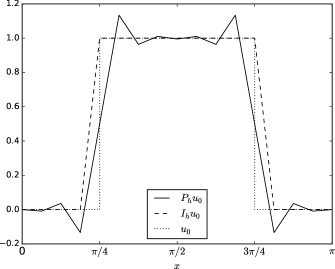
Figure 1: The $L_{2}$-projection $P_{h}u_{0}$ and the nodal interpolant $I_{h}u_{0h}$ of the discontinuous initial data (32) when $Q_{h}=15$.

6.1 Dirichlet boundary condition

In our first example, $F(x,t)=-x+\sin t$, $T=1$ and $\Omega=(0,\pi)$, with homogeneous Dirichlet boundary conditions $u(0,t)=0=u(\pi,t)$ and discontinuous initial data given by

$$u_{0}(x)=\begin{cases}1,\quad x\in[\pi/4,3\pi/4]\\ 0,\quad x\in[0,\pi/4)\cup(3\pi/4,1];\end{cases}$$ (32)

Figure 1 shows $u_{0}$ and its $L_{2}$-projection $P_{h}u_{0}$, as well as the nodal interpolant $I_{h}u_{0}\in\mathbb{S}_{h}$ defined by

$$I_{h}u_{0}(x_{p})=\begin{cases}1,\quad x_{p}\in[\pi/4,3\pi/4]\\ 0,\quad x_{p}\in[0,\pi/4)\cup(3\pi/4,1].\end{cases}$$ (33)

The Dirichlet eigenvalues and orthonormal eigenfunctions of $-\nabla^{2}=-\partial_{x}^{2}$ are

$$\lambda_{m}=m^{2}\quad\text{and}\quad\varphi_{m}(x)=\biggl{(}\frac{2}{\pi}\biggr{)}^{1/2}\,\sin mx\quad\text{for $m\in\{1,2,3,\ldots\}$,}$$

so for $0\leq r<1/2$ we have

$$\|u_{0}\|_{r}^{2}=\sum_{m=1}^{\infty}m^{2r}\langle u_{0},\varphi_{m}\rangle^{2}=\frac{4}{\pi}\sum_{j=1}^{\infty}(2j-1)^{2(r-1)}\leq\frac{C}{1-2r}.$$

If our conjecture that $K_{r}=C\|u_{0}\|_{r}$ in (8) is valid, then applying Theorem 5.1 with $r=\tfrac{1}{2}-\epsilon$ and $\epsilon^{-1}=\log(e^{2}+t^{-1})$, so that $t^{-\epsilon}\leq e$ and $0<\epsilon<1/2$, gives

$$\|u_{h}(t)-u(t)\|\leq C\|u_{0h}-P_{h}u_{0}\|+Ct^{-3\alpha/4}h^{2}\sqrt{\log(e^{2}+t^{-1})}\quad\text{for $0<t\leq 1$.}$$ (34)

In our computations, we employed nonuniform time levels given by (31), but a uniform spatial mesh with $h=1/(Q_{h}+1)$. In all cases, $Q_{h}+1$ was divisible by $4$ so that the points $\pi/4$ and $3\pi/4$ (where $u_{0}$ is discontinuous) coincided with two of the nodes. We first computed a reference solution $U_{\text{ref}}^{n}=U^{n}_{h}$ using a fine mesh with $N=10,000$ and $Q_{h}=511$. We then computed $U^{n}_{h}$ for $Q_{h}\in\{7,15,31,63\}$, again with $N=10,000$. The initial data was chosen as $u_{0h}=P_{h}u_{0}$ in each case. With such a small $k$, the error,

$$E_{h,k}^{n}=\|U^{n}_{h}-U_{\text{ref}}^{n}\|\quad\text{for $1\leq n\leq N$,}$$

was dominated by the influence of the spatial discretisation, and we sought to estimate the convergence rates $\sigma_{h,k}$ such that

$$E^{*}_{h,k}=\max_{0\leq n\leq N}\frac{t_{n}^{3\alpha/4}E_{h,k}^{n}}{\sqrt{\log(e^{2}+t_{n}^{-1})}}\approx Ch^{\sigma_{h,k}},$$ (35)

from the relation

$$\sigma_{h,k}=\log_{2}(E^{*}_{2h,k}/E^{*}_{h,k}).$$ (36)

Table 1 shows the values of $E^{*}_{h,k}$ and $\sigma_{h,k}$ for three different values of $\alpha$. The computed values of $\sigma_{h,k}$ are close to $2$, as expected from Theorem 5.1. Figure 2 shows how the $L_{2}$-error $E_{h,k}^{n}$ varies with $t_{n}$ for different $h$ when $\alpha=0.75$, again keeping $N=10,000$. Due to the log-log scale, the graph of a function proportional to $t^{-3\alpha/4}$ appears as a straight line with gradient $-3\alpha/4$, indicated by the small triangle, and we observe exactly this behaviour of the error for $t$ close—but not too close—to zero.

Table 1: Weighted errors (35) and convergence rates (36) for different $\alpha$, when $u_{0h}=P_{h}u_{0}$.

$Q_{h}$	$\alpha=0.25$		$\alpha=0.50$		$\alpha=0.75$
7	7.98e-03		7.77e-03		7.84e-03
15	1.96e-03	2.024	1.91e-03	2.024	1.94e-03	2.017
31	4.88e-04	2.008	4.75e-04	2.008	4.82e-04	2.007
63	1.21e-04	2.014	1.18e-04	2.014	1.19e-04	2.015

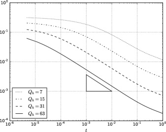
Figure 2: Plots of the error $E^{n}_{h,k}$ as a function of $t_{n}$, for $\alpha=0.75$ and different choices of $Q_{h}$. The triangle indicates the gradient $-3\alpha/4$ for a function proportional to $t^{-3\alpha/4}$; cf. (34). Note the logarithmic scales.

Table 2: Weighted errors (35) and convergence rates (36) for different $\alpha$, when $u_{0h}=I_{h}u_{0}$.

$Q_{h}$	$\alpha=0.25$		$\alpha=0.50$		$\alpha=0.75$
7	7.79e-02		7.46e-02		7.27e-02
15	4.04e-02	0.948	3.86e-02	0.950	3.76e-02	0.952
31	2.06e-02	0.973	1.97e-02	0.973	1.91e-02	0.974
63	1.04e-02	0.987	9.93e-03	0.987	9.65e-03	0.987

Physically, the solution $u$ must be non-negative, but the oscillations in the discrete initial data $P_{h}u_{0}$ mean that $U^{n}_{h}(x)$ was negative for some values of $(x,t_{n})$ near the points of discontinuity $(\pi/4,0)$ and $(3\pi/4,0)$. It is tempting to choose as the discrete initial data $u_{0h}=I_{h}u_{0}$, the nodal interpolant (33). In this way, $U^{0}_{h}=u_{0h}(x)\geq 0$ for all $x$. However, since

$$\langle u_{0h}-P_{h}u_{0},\chi\rangle=\langle u_{0h}-u_{0},\chi\rangle\leq\|u_{0h}-u_{0}\|\|\chi\|\quad\text{for all $\chi\in\mathbb{S}_{h}$,}$$

by choosing $\chi=u_{0h}-P_{h}u_{0}$ we see that

$$\|u_{0h}-P_{h}u_{0}\|\leq\|u_{0h}-u_{0}\|=\sqrt{\tfrac{2}{3}}\,h\quad\text{when $u_{0h}=I_{h}u_{0}$.}$$

Thus, Theorem 5.1 now yields an error bound of order $h+t^{-3\alpha/4}h^{2}$ (ignoring the log factor), and Table 2 indeed shows only first-order convergence for this choice of initial data.

At the end of Section 4, we remarked that in our stability estimate the constant tends to infinity as $\alpha$ approaches $1$. Since the finite element method is stable in the classical case $\alpha=1$, we suspect that the dependence of the stability constant on $\alpha<1$ is an artefact of the method of proof. To investigate this question numerically, we computed $\|u_{h}(t)\|$ for random initial data, that is, when the value of $u_{0h}$ at each node was a random number from a uniform distribution in $[0,1]$. In practice, we did not observe any deterioration in the stability of the method for $\alpha$ close to $1$.

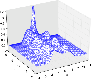
Figure 3: Surface plot of a solution using the potential (37) and imposing the zero-flux boundary condition (10); the part of the surface where $t<0.005$ is omitted.

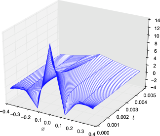
Figure 4: Detail of the surface plot showing the spurious oscillations for $(x,t)$ near the singularity at $(0,0)$.

6.2 Zero-flux boundary condition

In our second example,

$$F(x,t)=-\frac{\partial V}{\partial x},\quad\alpha=0.75,\quad T=20,\quad\Omega=(-L,L),\quad L=4,$$

where $V$ is a double-well potential perturbed by an oscillation in time,

$$V(x,t)=\tfrac{1}{4}x^{4}-\tfrac{1}{2}x^{2}-x\cos t.$$ (37)

Gammaitoni et al. GammaitoniEtAl1998 used this potential for the classical Fokker–Planck equation ($\alpha=1$) in their study of stochastic resonance. We imposed the zero-flux boundary condition (10) and chose as the initial data $u_{0}(x)=\delta(x)$. The solution $u$ then gives the probability distribution for a single diffusing particle initially located at $x=0$. Since the Dirac delta functional does not belong to $L_{2}(\Omega)$, our stability result (Theorem 4.1) does not apply, and $P_{h}u_{0}$ is not defined. Nevertheless, the functions in $\mathbb{S}_{h}$ are continuous, so by extending the $L_{2}$ inner product to a dual pairing we can define the discrete initial data $u_{0h}\in\mathbb{S}_{h}$ by

$$\langle u_{0h},\chi\rangle=\langle u_{0},\chi\rangle=\langle\delta,\chi\rangle=\chi(0)\quad\text{for all~{}$\chi\in\mathbb{S}_{h}$.}$$

Figure 3 shows a surface plot of the numerical solution using $N=\text{4,096}$ time steps, now with a stronger mesh grading $\gamma=2$ in (31), and $Q_{h}=65$ spatial degrees of freedom. (Thus the delta function is centred on the node $\vec{x}_{33}=0$). We cut off the initial part of the plot where $t<0.005$ to avoid the oscillations, shown separately in Figure 4, which are much larger than was the case for our first example. The total mass should be constant and we observed in practice that $\int_{\Omega}U^{n}_{h}=1$ to ten significant figures, for $0\leq n\leq N$.

References

- (1) C. N. Angstmann, I. C. Donnelly, B. I. Henry, T. A. M. Langlands and P. Straka, Generalised continuous time random walks, master equations and fractional Fokker–Planck equations, SIAM J. Appl. Math., 75 (2015), 1445–1468.
- (2) X. N. Cao, J.-L. Fu and H. Huang, Numerical method for the time fractional Fokker–Planck equation, Adv. Appl. Math. Mech., 4 (2015), 848–863.
- (3) S. Chen, F. Liu, P. Zhuang and V. Anh, Finite difference approximations for the fractional Fokker–Planck equation, Appl. Math. Model., 33 (2009), 256–273.
- (4) Mingrong Cui, Compact exponential scheme for the time fractional convection-diffusion reaction equation with variable coefficients, J. Comput. Phys., 280 (2015), 143–163.
- (5) Weihua Deng, Numerical algorithm for the time fractional Fokker–Planck equation, J. Comput. Phys., 227 (2007) 1510–1522.
- (6) J. Dixon and S. McKee, Weakly singular Gronwall inequalities, ZAMM Z. Angew. Math. Mech., 66 (1986), 535–544.
- (7) G. Fairweather, H. Zhang, X. Yang and D. Xu, A backward Euler orthogonal spline collocation method for the time-fractional Fokker–Planck equation, Numer. Meth. PDEs, 31 (2015), 1534–1550.
- (8) Luca Gammaitoni, Peter Hänggi, Peter Jung and Fabio Marchesoni, Stochastic resonance, Reviews of Modern Physics, 70 (1998), 223–285.
- (9) Guang-Hua Gao and Hai-Wei Sun, Three-point combined compact alternating direction implicit difference schemes for two-dimensional time-fractional advection-diffusion equations, Commun. Computat. Phys., 17 (2015), 487–509.
- (10) Guang-Hua Gao and Hai-Wei Sun, Three-point combined compact difference schemes for time-fractional advection–diffusion equations with smooth solutions, J. Comput. Phys, 298 (2015), 520–538.
- (11) José Luis Gracia and Eugene O’Riordan and Martin Stynes, Error analysis of a finite difference method for a time-fractional advection-diffusion equation, (2015.
- (12) E. Heinsalu, M. Patriarca, I. Goychuk and P. Hänggi, Use and abuse of a fractional Fokker–Planck dynamics for time-dependent driving, Phys. Rev. Lett., 99 (2007), 120602.
- (13) B. I. Henry, T. A. M. Langlands and P. Straka, Fractional Fokker–Planck equations for subdiffusion with space- and time-dependent forces, Phys. Rev. Lett., 105 (2010), 170602.
- (14) Yingjun Jiang, A new analysis of stability and convergence for finite difference schemes solving the time fractional Fokker–Planck equation, Appl. Math. Model., 39 (2015), 1163–1171.
- (15) Kim Ngan Le, William McLean and Kassem Mustapha, Numerical solution of the time-fractional Fokker–Planck equation with general forcing, SIAM J. Numer. Anal., 54, (2016), 1763–1784.
- (16) William McLean, Regularity of solutions to a time-fractional diffusion equation, ANZIAM J., 52 (2010), 123–138.
- (17) Richard K. Miller and Alan Feldstein, Smoothness of solutions of Volterra integral equations with weakly singular kernels, SIAM J. Math. Anal., 2 (1971), 242–258.
- (18) Kassem Mustapha and Dominik Schötzau, Well-posedness of -version discontinuous Galerkin methods for fractional diffusion wave equations, IMA J. Numer. Anal., 34 (2014), 1426–1446.
- (19) Abbas Saadatmandi, Mehdi Dehghan and Mohammad-Reza Azizi, The Sinc–Legendre collocation method for a class of fractional convection–diffusion equations with variable coefficients, Commun. Nonlinear Sci. Numer. Simul., 17 (2012), 4125–4136,
- (20) Seakweng Vong and Zhibo Wang, A high order compact finite difference scheme for time fractional Fokker–Planck equations, Appl. Mat. Lett., 43 (2015), 38–43.
- (21) Leilei Wei, Xindong Zhang and Yinnian He, Analysis of a local discontinuous Galerkin method for time-fractional advection-diffusion equations, Internat. J. Numer. Methods Heat Fluid Flow, 23 (2013), 634–648.
- (22) Minling Zheng, Fawang Liu, Ian Turner and Vo Anh, A novel high order space-time spectral method for the time fractional Fokker–Planck equation, SIAM J. Sci. Comput., 37 (2015), A701–A724.