Robust Streaming PCA

Abstract

We consider streaming principal component analysis when the stochastic data-generating model is subject to perturbations. While existing models assume a fixed covariance, we adopt a robust perspective where the covariance matrix belongs to a temporal uncertainty set. Under this setting, we provide fundamental limits on convergence of any algorithm recovering principal components. We analyze the convergence of the noisy power method and Oja’s algorithm, both studied for the stationary data generating model, and argue that the noisy power method is rate-optimal in our setting. Finally, we demonstrate the validity of our analysis through numerical experiments on synthetic and real-world dataset.

1 Introduction

Principal component analysis (PCA) is one of the most extensively studied methods for obtaining the low-dimensional representation of observed data [22]. However, classical algorithms for PCA store all the observations and use cubic-time complexity, thereby imposing prohibitively large computation-time and space requirements.

Recently, several works on PCA have focused on the design and analysis of streaming algorithms with near-optimal memory and storage complexity [40, 43, 25, 29]. These algorithms assume that all the observations belong to the same low-dimensional space. However, this situation is unlikely when the unknown/unexplored alterations corrupt a system’s observations. For instance, it is well known that typical data attacks on power grids can significantly change the estimated covariance matrix of the data observed from sensors [9, 23, 10]. Similarly, PCA can be used to explain stock returns in terms of macroeconomic factors [27], and product pricing taking into account cross-product elasticity and demands [45]. In all these scenarios, the underlying data-generating model changes every instant, and the decisions are based on identifying the changed model.

Current work considers perturbations of the data lying in a fixed low-dimensional space [49]. They determine the worst-case position of the adversarial data point to incur the maximum error in the subspace estimated through PCA and measure the distance between the two subspaces using the notion of the principal angle between them. Another line of work considers PCA through the lens of stochastic optimization [51, 52, 42, 5]. Our work differs from these approaches since we assume that the data-generating model changes at every time instant. Further, we propose near-optimal algorithms for recovering principal components under this framework.

We assume a system relies on the time-series of $p$-dimensional vectors sampled from a time-varying model. The available observations are the vectors $(\mathbf{x}_{t})_{t=1}^{T}$. The noisy observation $\mathbf{x}_{t}\in\mathbb{R}^{p}$ is a vector lying in the column space of an unobserved full-rank matrix $\mathbf{A}_{t}\in\mathbb{R}^{p\times k}$. Precisely, from the standard spiked covariance model [35], we consider the time-dependent environment:

$$\mathbf{x}_{t}\sim\mathcal{N}(\mathbf{0}_{p\times 1}\,,\,\mathbf{\mathbf{A}}_{t}\mathbf{\mathbf{A}}^{\top}_{t}+\sigma^{2}\mathbf{I}_{p\times p}),$$ (1)

where $\mathbf{A}_{t}$ can vary with time. The parameter $k\ll p$ is the desired number of principal components. Assuming $\mathbf{A}_{t}$ belongs to a temporal uncertainty set (defined in the equation (2)), our goal is to recover the top-$k$ principal components of the terminal subspace $\mathbf{A}_{T}$. In financial applications, our model captures the market evolution in terms of the changing $\mathbf{A}_{T}$ with the ultimate goal of explaining the market conditions for an appropriately chosen $T$.

Previous works on the stationary environment assume $\mathbf{A}_{t}\!=\!\mathbf{A}$ for all $t$ and have focused on computing a basis for the column space of the matrix $\mathbf{A}$ using streaming algorithms [43, 29, 38, 33, 21, 36]. The accurate reconstruction of the principal components for the standard streaming PCA problem depends on the magnitude of observation noise $\sigma$, the dimension of observations $p$, the number of principal components $k$ of the matrix $\mathbf{A}$, and the spectral gap $\delta$ between $k$-th and $k\!+\!1$-th spectrums. singular value of $\mathbf{A}\mathbf{A}^{\top}$. In a marked departure from previous work, we study the case when the column space of $\mathbf{A}$ varies across time. This paper explores these avenues and proposes a tractable analysis framework for the streaming PCA problem, robust to perturbations in the data-generating model. Our contributions can be summarized as follows:

1. (Lower Bound; Section 4) Our first contribution is establishing a fundamental lower bound for estimating the principal components when the covariance matrix belongs to a temporal uncertainty set $\textup{Tu}(\delta,\Gamma)$. In Theorem 1, we derive the minimax bounds of the expected error for recovering the top singular vectors for any streaming algorithm. Because the underlying distribution can vary, observations from the far past become less important and the estimation of principal components associated with $\mathbf{A}_{T}$ should be determined by a subset of samples. Simultaneously, it becomes imperative to find the block size $B$ that can be used to recover the principal components. This is in sharp contrast to the standard spiked covariance model. We show that:

   • For $T\!=\!\mathcal{O}(\Gamma^{\shortminus 2/3})$, the minimax estimation error decreases as $\mathcal{O}({p^{1/2}}T^{\shortminus 1/2})$.

   • On the other hand, for $T\!=\!\Omega(\Gamma^{\shortminus 2/3})$, the error stagnates to $\mathcal{O}({p^{1/3}\Gamma^{1/3}})$ and does not decrease upon collecting more observations.

2. (Algorithm Analysis; Section 5) We then analyze two algorithms to recover the principal components extensively used in the standard streaming PCA setting; the noisy power method [29] and Oja’s algorithm [48]. These algorithms represent two very different design principles for computing principal components from data in streaming fashion, processing data in blocks vis-à-vis single observations. We determine the optimal choice for critical parameters: the block size in the noisy power method on Lemma 1 and the learning rate in Oja’s algorithm on Lemma 2. Next, we leverage these results to obtain an upper bound on the convergence error for these algorithms in Theorem 2 and 3, respectively. From these results, we have:

   • The block size $B$ for the noisy power method and inverse of the learning rate, $\zeta^{-1}$ for Oja’s algorithm, plays a similar role even in the non-stationary environment. In either case, the optimal parameters scale with $\Theta(\Gamma^{-2/3})$, where $\Gamma$ is the perturbation budget.

   • The derived upper bound on the estimation error for the noisy power method matches the minimax error in terms of $p,\delta,$ and $\Gamma$ and becomes rate-optimal if it satisfies the mild conditions.

Notation. We fix notation throughout the main body of the paper. Matrices are denoted by bold uppercase letters (e.g. $\mathbf{M}$) and vectors are denoted by bold lowercase letters (e.g. $\mathbf{x}$). For $\mathbf{M}\in\mathbb{R}^{p\times k}$, $\mathbf{M}_{i}$ denote the $i{\mathrm{th}}$ column of $\mathbf{M}$, $\mathbf{M}_{i:j}$ denote the submatrix consists with $i{\mathrm{th}}\!\sim\!j{\mathrm{th}}$ column of $\mathbf{M}$ and $\mathbf{M}_{i,j}$ be the $(i,j)$-element of $\mathbf{M}$. $\lVert\,\cdot\,\rVert$ denote matrix 2-norm or equivalently operator norm for matrices and standard 2-norm for vectors. We use ${\mathrm{St}}_{k}(\mathbb{R}^{p})$ for the class of orthogonal matrices in $\mathbb{R}^{p\times k}$. $b(\mathbf{M})$ is the orthogonal matrix where the columns form basis for $\mathrm{ran}(\mathbf{M})$. $s_{i}(\mathbf{M})$ represents the $i{\mathrm{th}}$ largest singular value of the matrix.

The singular value decomposition of $\mathbf{M}$ is defined as $\mathrm{SVD}(\mathbf{M})\!=\!\mathbf{U}\mathbf{D}\mathbf{V}^{\top}$, where $\mathbf{U}\!\in\!{\mathrm{St}}_{p}(\mathbb{R}^{p})$, $\mathbf{V}\!\in\!{\mathrm{St}}_{k}(\mathbb{R}^{k})$, and $\mathbf{D}\!\in\!\mathbb{R}^{p\times k}$ is a diagonal matrix whose $i{\mathrm{th}}$ diagonal element equals $s_{i}(\mathbf{M})$. Therefore, we assume without loss of generality that the singular values and respective singular vectors are ordered from largest to smallest. We denote by $\mathbf{M}_{\perp}$ the orthogonal projection onto the orthogonal complement of the $\mathrm{ran}(\mathbf{M})$. Therefore, if $\mathrm{rk}(\mathbf{M})\!=\!r$ and $\mathrm{SVD}(\mathbf{M})\!=\!\mathbf{U}\mathbf{D}\mathbf{V}^{\top}$, $\mathbf{M}_{\perp}$ given by $\mathbf{M}_{\perp}\!=\!\mathbf{I}-\mathbf{\mathbf{U}}_{1:r}\mathbf{\mathbf{U}}^{\top}_{1:r}$. Moreover, when $\mathrm{rk}(\mathbf{M})\!=\!\mathrm{rk}(\tilde{\mathbf{M}})$ and $\mathrm{SVD}(\tilde{\mathbf{M}})\!=\!\tilde{\mathbf{U}}\tilde{\mathbf{D}}\tilde{\mathbf{V}}^{\top}$, the distance between $\mathrm{ran}(\mathbf{M})$ and $\mathrm{ran}(\tilde{\mathbf{M}})$ is defined by:

$$d(\mathrm{ran}(\mathbf{M}),\mathrm{ran}(\tilde{\mathbf{M}}))=\lVert\>b(\mathbf{M})b(\mathbf{M})^{\top}-b(\tilde{\mathbf{M}})b(\tilde{\mathbf{M}})^{\top}\>\rVert=\lVert\>\mathbf{\mathbf{U}}_{1:k}\mathbf{\mathbf{U}}^{\top}_{1:k}-\mathbf{\tilde{\mathbf{U}}}_{1:k}\mathbf{\tilde{\mathbf{U}}}^{\top}_{1:k}\>\rVert\,.$$

We denote $d(\mathrm{ran}(\mathbf{M}),\mathrm{ran}(\tilde{\mathbf{M}}))$ by $d(\mathbf{M},\tilde{\mathbf{M}})$ whenever clear from the context.

The letter $\mathcal{A}$ stands for abbreviation of sequence of matrices $(\mathbf{A}_{t})_{t=1}^{T}$. We write $\mathcal{X}\!\!\sim\!\!\mathcal{A}$ when each element $\mathbf{x}_{t}$ in sequence $\mathcal{X}=$ $(\mathbf{x}_{t})_{t=1}^{T}$ are drawn from $\mathcal{N}(\mathbf{0},\mathbf{\mathbf{A}}_{t}\mathbf{\mathbf{A}}^{\top}_{t}+\sigma^{2}\mathbf{I}_{p\times p})$. We denote the expectation of $f(\mathcal{X})$ over $\mathbf{x}_{t}\sim\mathcal{N}(\mathbf{0},\mathbf{\mathbf{A}}_{t}\mathbf{\mathbf{A}}^{\top}_{t}+\sigma^{2}\mathbf{I}_{p\times p})$ as $\mathbb{E}_{\mathcal{X}\sim\mathcal{A}}\,[f]$.

We denote $\tilde{\mathcal{O}}$, $\tilde{\Theta}$ as the $\mathcal{O}$, $\Theta$ notation with ignore the multiplicative dependency of $\log(pT^{2})$ or smaller.

2 Related Work

Principal component analysis (PCA) has been extensively studied across operations research, computer science, and other communities. We highlight how our work differs from existing literature.

Robust PCA. Robust PCA deals with the problem of retrieving the principal components robust to the presence of outliers in the data. The cornerstone work in this direction is the principal component pursuit framework wherein they assume that the matrix of observations $\mathbf{M}$ can be decomposed in terms of a low-rank matrix $\mathbf{L}$ and a sparse matrix (with entries of arbitrarily large magnitude) $\mathbf{S}$ [15].

Several works consider the robust PCA problem and propose algorithms in the offline, batch, and online settings [24, 26, 17, 46]. Our work differs from this line of literature in two aspects: assumptions about the data-generating model and convex optimization techniques. First, our data generation model is unrelated to those considered in the robust PCA literature. Further, rich theories from convex optimization can be used in the PCA framework to design efficient algorithms, but our problem is not amenable to such techniques.

Streaming PCA. Streaming algorithms for PCA have been proposed, among other works on PCA [43, 34, 29, 60, 2]. Algorithms analyzed in this work, such as the noisy power method [29] and Oja’s algorithm [48], are iterative methods for estimating the principal components. These iterative schemes are instances of stochastic approximation-based solutions for the optimization formulation of the PCA problem [5]. The stochastic approximation is a root-finding framework extensively used for stochastic optimization [37, 11]. Oja’s algorithm, originally proposed by [48], was the first such scheme.

This framework is also used to analyze gradient-type and proximal-type incremental methods akin to algorithms for convex optimization. Stochastic gradient descent-based algorithms for the streaming PCA problem, where a single observation is used at every point in time to update the principal components’ estimate, have been extensively studied. Along this line, [30] propose GRASTA, an incremental online gradient method for learning over different subspaces. Similarly, [6] proposes GROUSE, based on the idea of gradient updates over the Grassmannian manifold. These and other related works consider Oja’s algorithm for the standard streaming PCA problem [53, 16, 62, 31, 31, 1, 59]. However, all these works are based on a completely different modeling assumption than this paper and do not provide theoretical guarantees for our setting.

Streaming and robust PCA algorithms are used in the presence of outliers or data with a lot of missing entries [18, 55]. From this literature, the closest to our work is the work on robust subspace tracking [2, 60, 30]. However, the robustness considered there is against erasures or sparse outliers. While these algorithms provide theoretical guarantees in that setting, those guarantees cannot be extended to our model. Considerations of erasures and outliers under the model proposed in this paper are beyond the scope of this work and remain an interesting future direction.

3 Mathematical Framework

Observations from the standard spiked covariance model belong to a fixed $k$-dimensional column space $\mathbf{A}\in\mathbb{R}^{p}$. Previous work has focused on reconstructing this space from the observed time series. Under our framework, we assume that the sequence of observations $(\mathbf{x}_{t})_{t=1}^{T}$ follows the time-dependent spiked covariance model (1). We consider the problem of computing top-$k$ singular vectors of $\mathbf{A}_{T}$. We formulate this model by addressing minimax optimization as a robust optimization problem.

When the adversary is allowed to select a completely arbitrary sequence of matrices $(\mathbf{A}_{t})_{t=1}^{T}$, it is impossible to accurately recover the column space of $\mathbf{A}_{T}$. Instead, we define temporal uncertainty sets to restrict the power of the adversary.

Definition 1.

Let $\Gamma,\delta\geq 0$. We only allow the sequence of matrices $(\mathbf{A}_{t})_{t=1}^{T}$ that lie in an temporal uncertainty set $\textup{Tu}(\delta,\Gamma)$ defined as:

$$\textup{Tu}(\delta,\Gamma):=\big{\{}\,(\mathbf{A}_{t})_{t=1}^{T}\>:\>s_{k}(\mathbf{\mathbf{A}}_{t}\mathbf{\mathbf{A}}^{\top}_{t})\geq\delta\>,\>\|\mathbf{\mathbf{A}}_{t}\mathbf{\mathbf{A}}^{\top}_{t}-\mathbf{\mathbf{A}}_{t-1}\mathbf{\mathbf{A}}^{\top}_{t-1}\|\leq\Gamma,\big{\}}\,.$$ (2)

We constrain the difference between any two consecutive covariance matrices of the underlying process by $\Gamma$. The assumption $s_{k}(\mathbf{\mathbf{A}}_{t}\mathbf{\mathbf{A}}^{\top}_{t})\geq\delta$ is crucial for establishing bounds of estimation error. It is also justified in any setting where the underlying phenomenology guarantees covariance of rank k; the stated lower bound excludes pathological cases of near-rank $k\!-\!1$ or smaller.

Having described the constraints on the perturbation power, we present the algorithms and the performance metric of interest. In particular, we consider (i) streaming algorithms, i.e., make a single pass through the time series in chronological order; only the previous samples are stored at any point in the past. These characteristics model the behavior of an algorithm that receives data in real-time and only stores samples in limited memory. Among those streaming algorithms, we consider (ii) the algorithms whose output is a set of $k$ orthonormal vectors in $\mathbb{R}^{p}$. Let us denote by $\Phi$ the family of algorithms just described. The output of algorithm $\phi\in\Phi$ for a given observations $\mathcal{X}=(\mathbf{x}_{t})_{t=1}^{T}$ sampled using model (2) is a set of $k$ orthonormal vectors, which we denote by $\phi_{\mathcal{X}}$. We will also view $\phi_{\mathcal{X}}$ as a matrix in $\mathbb{R}^{p\times k}$ or the subspace generated by $\phi_{\mathcal{X}}$.

Following definition 2 illustrates how we treat the lower bound and when we call the algorithm optimal. We note that this formulation has been widely studied [57, 14, 58].

Definition 2.

Let $\mathcal{A}=(\mathbf{A}_{t})_{t=1}^{T}\in\textup{Tu}(\delta,\Gamma)$, and $\phi\in\Phi$.

1. The estimation error of $\phi$ given $\mathcal{X}\sim\mathcal{A}$ is the distance between the space spanned by $\phi_{\mathcal{X}}$ and the column space of $\mathbf{A}_{T}$ ($d(\text{ran}(\mathbf{A}_{T}),\phi_{\mathcal{X}})$). The metric can be easily extended to the cumulative error. Refer Appendix A for the discussion.

2. $\mathcal{R}^{\phi}$ is the maximum expected estimation error of $\phi$ under $\mathcal{A}$ over all $\mathcal{A}\in\textup{Tu}(\delta,\Gamma)$.

   $$\mathcal{R}^{\phi}\>:=\sup_{\mathcal{A}\in\textup{Tu}(\delta,\Gamma)}\mathbb{E}_{\mathcal{X}\sim\mathcal{A}}\big{[}d\big{(}\text{ran}(\mathbf{A}_{T}),\phi_{\mathcal{X}}\big{)}\big{]}\,.$$

3. $\mathcal{R}^{\ast}$ is the minimax estimation error defined as the minimum of the largest expected estimation error incurred by $\phi\in\Phi$:

   $$\mathcal{R}^{\ast}:=\inf_{\phi}\mathcal{R}^{\phi}=\inf_{\phi}\sup_{\mathcal{A}\in\textup{Tu}(\delta,\Gamma)}\mathbb{E}_{\mathcal{X}\sim\mathcal{A}}\big{[}d\big{(}\text{ran}(\mathbf{A}_{T}),\phi_{\mathcal{X}}\big{)}\big{]}\,.$$

4. An algorithm $\phi\in\Phi$ is rate-optimal if $\mathcal{R}^{\phi}\leq C\cdot\mathcal{R}^{\ast}\,$, where constant $C>0$ is independent of the problem parameters $T$, $\delta$, $p$, $k$, and $\Gamma$.

In this work, we establish the minimax estimation error $\mathcal{R}^{\ast}$ and propose rate-optimal sublinear-time, single-pass algorithms for robust streaming PCA.

4 Minimax Lower Bound

When $\mathcal{A}=(\mathbf{A}_{t})_{t=1}^{T}$ belongs to the temporal uncertainty set $\textup{Tu}(\delta,\Gamma)$ (Definition 1), an algorithm designed to recover the principal components of $\mathbf{A}_{T}$ from the observations cannot guarantee zero estimation error. Our first goal is to obtain the minimax lower bound on the estimation error in the problem parameters $T$, $\delta$, $p$, $k$, and $\Gamma$.

In order to establish the lower bound, we leverage the fundamental limit of hypothesis tests [57]. The crux of the proof lies in constructing the set of worst-case hypotheses and establishing a lower bound on the probability of error in distinguishing between these hypotheses using observed data. The complete proof is provided in Appendix D.

Theorem 1 (Lower Bound).

Assume $\delta>\Gamma\geq 0$ and $p>2k+1$. For any algorithm $\phi\in\Phi$, there exists a sequence $\mathcal{A}\in\textup{Tu}(\delta,\Gamma)$ such that $\mathbb{E}_{\mathcal{X}\sim\mathcal{A}}\big{[}d\big{(}\mathrm{ran}(\mathbf{A}_{T}),\phi_{\mathcal{X}}\big{)}\big{]}$ has lower bound with order:

$$\Theta\left(\min\left\{1\,,\frac{1}{\sqrt{T}}\left(\frac{p\sigma^{2}(\sigma^{2}+\delta)}{\delta^{2}}\right)^{{1}/{2}}\!\!+\,\,\underline{\left(\frac{\Gamma}{\delta}\right)^{{1}/{3}}\left(\frac{p\sigma^{2}(\sigma^{2}+\delta)}{\delta^{2}}\right)^{{1}/{3}}}\,\right\}\right).$$ (3)

By taking $\inf_{\phi\in\Phi}$, we get the same lower bound for $\mathcal{R}^{*}$.

For the standard streaming PCA problem (Theorem 1 with the case of $\Gamma\!=\!0$), the fundamental limit is $\Theta((\sigma/\delta)({p(\sigma^{2}+\delta)}/{T})^{1/2})$ , which has the expected $\Theta({1}/{\sqrt{T}})$ dependence [14, 58]. On the other hand, in the presence of perturbations ($\Gamma\!>\!0$), the lower bound exhibits a phase transition phenomenon, with the first term representing the effect of model ambiguity. To this end, define the critical time $T_{c}$ as

$$T_{c}:=\left(\frac{\Gamma}{\delta}\right)^{-{2}/{3}}\left(\frac{p\sigma^{2}(\sigma^{2}+\delta)}{\delta^{2}}\right)^{{1}/{3}}\,.$$ (4)

For $T\!=\!\mathcal{O}(T_{c})$, the lower bound decreases with the rate of $1/\sqrt{T}$. However, when $T\!=\!\Omega(T_{c})$, the first term dominates the second term, and $\mathcal{R}^{\ast}$ becomes independent of the number of observations $T$. In this regime, the error stagnates to $\mathcal{O}(({\Gamma}/{\delta})^{{1}/{3}}\left({p\sigma^{2}(\sigma^{2}+\delta)}/{\delta^{2}}\right)^{{1}/{3}})$. Therefore, as our intuition suggests, the information quickly becomes stale in a dynamic environment.

Theorem 2 and 3 will prove that the noisy power method and Oja’s algorithm attain a near-optimal bound on the convergence guarantee. Theorem 2 guarantees that if $s_{1}(\mathbf{\mathbf{A}}_{t}\mathbf{\mathbf{A}}^{\top}_{t})=\Theta(\delta)$, the upper bound for estimation error on the noisy power method is of the following order:

$$\mathcal{R}^{\mathrm{NPM}}=\tilde{\mathcal{O}}\left(\Big{(}\frac{\Gamma}{\delta}\Big{)}^{1/3}\Big{(}\frac{(p\sigma^{2}+k\delta)(\sigma^{2}+\delta)}{\delta^{2}}\Big{)}^{1/3}\right)\,.$$ (5)

That is, if $p\sigma^{2}$ dominates $k\delta$, the noisy power method becomes rate-optimal under the controlled uncertainty with $\textup{Tu}(\delta,\Gamma)$. This regime is the case of noisy practical situations, with $\sigma^{2}\centernot\ll\delta$.

5 Convergence Analysis

In this section, we analyze two algorithms for the robust streaming PCA problem. A generic template for algorithms, $\phi\in\Phi$ of interest to us is as follows: (i) $\phi$ is initialized with a random matrix with orthonormal columns $\hat{\mathbf{U}}\in\mathbb{R}^{p\times k}$; (ii) a running estimate of the principal components is maintained as the columns of $\hat{\mathbf{U}}$; (iii) observations are projected onto the column space of $\hat{\mathbf{U}}$ to update this estimate.

We consider two algorithms: a robust version of the noisy power method (Algorithm 1) and Oja’s algorithm (Algorithm 2). The critical difference between the noisy power method and Oja’s algorithm is the data used to estimate the principal components. In the noisy power method, the estimates are updated after a batch of observations, whereas in Oja’s algorithm, the estimates are updated after scaling every observation with the learning rate. Therefore, the parameters determining the performance of these algorithms are the batch size $B$ for the robust power method and the learning rate $\zeta$ for Oja’s algorithm.

The analysis of these algorithms cannot be readily established with existing techniques when the covariance matrix belongs to a temporal uncertainty set since they rely on showing that the estimates improve every iteration. Further, applying many concentration results requires random matrices to be bounded, which is not the case when the observations are sampled from (1). Therefore, in order to simplify the analysis of both algorithms, we introduce Assumption 1, adapted from [34].

Assumption 1.

Let $(\mathbf{A}_{t})_{t=1}^{T}\in\textup{Tu}(\delta,\Gamma)$. For $\tilde{\delta}\geq\delta$ and $\mathcal{M},\mathcal{V}>0$, we consider the observations $\mathbf{x}_{t}$ for $t\in[T]$ satisfy the following:

1. $\mathbb{E}[\mathbf{\mathbf{x}}_{t}\mathbf{\mathbf{x}}^{\top}_{t}]=\mathbf{\mathbf{A}}_{t}\mathbf{\mathbf{A}}^{\top}_{t}+\sigma^{2}\mathbf{I}_{p\times p}$ while $\|\mathbf{\mathbf{A}}_{t}\mathbf{\mathbf{A}}^{\top}_{t}\|\leq\tilde{\delta}$,

2. $\|\mathbf{\mathbf{x}}_{t}\mathbf{\mathbf{x}}^{\top}_{t}-(\mathbf{\mathbf{A}}_{t}\mathbf{\mathbf{A}}^{\top}_{t}+\sigma^{2}\mathbf{I}_{p\times p})\|\leq\mathcal{M}$ a.s., and

3. $\left\lVert\mathbb{E}\left[(\mathbf{\mathbf{x}}_{t}\mathbf{\mathbf{x}}^{\top}_{t}-(\mathbf{\mathbf{A}}_{t}\mathbf{\mathbf{A}}^{\top}_{t}+\sigma^{2}\mathbf{I}_{p\times p}))^{2}\right]\right\rVert\leq\mathcal{V}$.

When the observations follow model (1), we condition our analysis on the high-probability event $\mathfrak{E}$.

Definition 3.

Let $\mathrm{SVD}(\mathbf{\mathbf{A}}_{t}\mathbf{\mathbf{A}}^{\top}_{t}+\sigma^{2}\mathbf{I}_{p\times p})\!=\!\mathbf{U}_{t}\mathbf{D}_{t}\mathbf{U}_{t}^{T}$ and $\mathbf{x}_{t}\!=\!\mathbf{U}_{t}\mathbf{D}_{t}^{1/2}\mathbf{z}_{t}$, where $\mathbf{z}_{t}\!\sim\!\mathcal{N}(\mathbf{0},\mathbf{I}_{p\times p})$. We define the event $\mathfrak{E}$ as:

$$\mathfrak{E}:=\left\{\mathbf{z}_{t}\in\left[-\sqrt{2\log(2pT^{2})},\sqrt{2\log(2pT^{2})}\right]^{\,p}\,;\,\forall t\in[T]\right\}\,.$$

The observations from model (1) satisfy Assumption 1 with $\mathcal{M}=2(k\tilde{\delta}+p\sigma^{2})(1+\Theta(\log(pT^{2})/T))$, $\mathcal{V}=2\mathcal{M}(\tilde{\delta}+\sigma^{2})$ with probability $\mathbb{P}[\mathfrak{E}]\geq 1-1/T$. Although after conditioning $\mathbb{E}[\mathbf{\mathbf{x}}_{t}\mathbf{\mathbf{x}}^{\top}_{t}|\mathfrak{E}]\neq\mathbf{\mathbf{A}}_{t}\mathbf{\mathbf{A}}^{\top}_{t}+\sigma^{2}\mathbf{I}_{p\times p}$, we can use all the results in Section 5.1 and 5.2 with a multiplicative logarithmic factor. Please refer to Appendix B for the details.

5.1 Noisy Power Method

Algorithm 1 Noisy Power Method with block size $B$ [29]

1:  Input: Stream of vectors: $(\mathbf{x}_{t})_{t=1}^{T}$, block size: $B$, dimensions: $p,k$

2:  Sample each element of $\mathbf{\hat{U}}(0)$ in $\mathcal{N}(0,1)$

3:  for $\ell=1:L=\lfloor T/B\rfloor$ do

4:     $\mathbf{Y}(\ell)\leftarrow\mathbf{0}\in\mathbb{R}^{p\times k}$

5:     for $t=(\ell-1)B+1:\ell B$ do

6:        $\mathbf{Y}(\ell)\leftarrow\mathbf{Y}(\ell)+\frac{1}{B}\mathbf{\mathbf{x}}_{t}\mathbf{\mathbf{x}}^{\top}_{t}\mathbf{\hat{U}}(\ell-1)$

7:     end for

8:     $\mathbf{\hat{U}}(\ell)\leftarrow\text{Gram-Schmidt}(\mathbf{Y}(\ell))$

9:  end for

10:  Output: $\mathbf{\hat{U}}(L)$

The noisy power method is an iterative algorithm for computing the top-$k$ principal components of a matrix. Starting from the random matrix $\hat{\mathbf{U}}(0)$ in $\mathbb{R}^{p\times k}$, the algorithm runs for $L$ iterations, each processing $B$ samples. By repeating this procedure, we expect the algorithm to reconstruct the covariance matrix if the observations are derived from the fixed distribution.

When observations are drawn from model (1) under Assumption 1, the later observation can be sampled from distributions with shifted covariance. Unlike the standard case, for any algorithm $\phi\in\Phi$, the presence of perturbation prevents the convergence of the columns of $\hat{\mathbf{U}}(\ell)$ to the singular vectors of the final covariance matrix $\mathbf{U}(\ell)$. The main difficulty here is that the columns of $\hat{\mathbf{U}}(\ell)$ do not converge towards a fixed set of vectors but keep tracking the time-varying principal components. Recall that our ultimate objective is to recover the principal components associated with the terminal observation. Hence, we decompose the covariance matrix in terms of the last observation and the remaining samples. For $\ell$-th block, we denote the covariance matrix for $\ell B$-th observation as $\mathbf{M}(\ell)$ and have:

$$\frac{1}{B}\>\sum_{\mathclap{t=(\ell-1)B+1}}^{\ell B}\>\mathbf{x}_{t}\mathbf{x}^{\top}_{t}=\>\mathbb{E}[\mathbf{x}_{\ell B}\mathbf{x}^{\top}_{\ell B}]+\mathbf{\mathcal{E}}(\ell)=\underbrace{\mathbf{A}_{\ell B}\mathbf{A}_{\ell B}^{\top}+\sigma^{2}\mathbf{I}}_{\mathbf{M}(\ell)}+\mathcal{E}(\ell)\,.$$ (6)

Due to perturbations in the robust model, $\mathcal{E}(\ell)$ is a non-zero mean random variable. Therefore, we first decompose $\mathcal{E}(\ell)$ in terms of the contribution due to inherent noise and the perturbations the robust model allows. Then, in Lemma 1, we decompose the error $\|\mathcal{E}(\ell)\|$ with respect to the block size $B$ and the allowed perturbations $\Gamma$ in the robust model. We provided complete proof in Appendix E.

Lemma 1 (Spectral norm of noise).

Assume that the observations $(\mathbf{x}_{t})_{t=1}^{T}$ generated according to the Assumption 1. With probability greater than $1-1/T$, the matrices $\mathcal{E}(\ell)$ in the equation (6) are bounded by:

$$\max_{1\leq\ell\leq L}\|\mathcal{E}(\ell)\|\leq\frac{1+3\sqrt{2}}{3}\sqrt{\frac{\mathcal{V}\log(2pT^{2})}{B}}+\frac{B\Gamma}{2}.$$ (7)

when the block size $B$ is larger than $\mathcal{M}^{2}\log(2pT^{2})/\mathcal{V}$.

Lemma 1 highlights the effect of allowing perturbations in the data generation model. From classical results in statistics, our intuition tells us that the effect of noise washes out as the block size increases, i.e., the error decays with the ‘inverse square root’ of the block size. Hence, barring memory and data issues, a larger block size is better when $\Gamma=0$. In contrast, covariance perturbations add errors proportional to the block size. Consequently, we have a trade-off between two terms in this case, and an optimal block size exists depending on the $\Gamma$.

We establish the convergence guarantee of the robust power method in Theorem 2. In the proof of Theorem 2 (Appendix F), we bound the distance, $d\big{(}\mathbf{U}(L),\hat{\mathbf{U}}(L)\big{)}$ between the output of Algorithm 1, $\hat{\mathbf{U}}_{1:k}(L)$ and $k$-orthonormal vectors spanning the column space of $\mathbf{A}_{T},\mathbf{U}_{1:k}(L)$. We identify the optimal block size $B$, the unique parameter for the noisy power method, and establish an upper bound on the estimation error of the noisy power method.

Theorem 2 (Robust power method).

Assume that $\delta\geq$ $0.71\sigma^{2}$ and $\Gamma=\mathcal{O}(\delta^{3}/(\mathcal{V}\log(2pT^{2})))$. When the observations $(\mathbf{x}_{t})_{t=1}^{T}$ satisfies the assumption 1, for $B=$ $\Theta(\mathcal{V}^{1/3}\log(2pT^{2})^{1/3}/{\Gamma^{2/3}})$ we have:

$$d(\mathrm{ran}(\mathbf{A}_{T}),\mathrm{NPM}_{\mathcal{X}})=\mathcal{O}\left(\frac{(\mathcal{V}\Gamma\log(2pT^{2}))^{1/3}}{\delta}\!+\!0.7^{{T}/{B}}\right)\,,$$ (8)

with probability $1-2/T-c^{\Omega(p-k+1)}-e^{-\Omega(p)}$.

When $\Gamma=\Omega(\delta^{3}/(\mathcal{V}\log(2pT^{2})))$ we have that $(\mathcal{V}\Gamma\log(2pT^{2}))^{1/3}/{\delta}=\Omega(1)$. Therefore, the condition on $\Gamma$ in Theorem 2 is necessary to avoid a trivial upper bound $\Theta(1)$. This condition encompasses several applications of interest alluded to earlier. For example, in the financial applications alluded to earlier, individual market changes of interest happen on a millisecond time scale. It is of significant interest to terminally detect incremental market changes. Our results hold on to the large value of cumulative changes and allow us to study them. They further imply that the noisy power method is rate-optimal for non-trivial values of $\Gamma$. When the observations follow model (1), under the event $\mathfrak{E}_{\Delta}$, Theorem 2 shows that the robust power method can achieve an estimation error of:

$$\mathcal{R}^{\mathrm{NPM}}=\tilde{\mathcal{O}}\left(\left(\frac{\Gamma}{\delta}\right)^{1/3}\left(\frac{(p\sigma^{2}+k\delta)(\sigma^{2}+\delta)}{\delta^{2}}\right)^{1/3}\right)\,,$$ (9)

if $T=\Omega(\max(T_{c}\,,\delta(p\sigma^{2})^{-1}))$, $\Gamma=\Omega((c^{\Omega(p-k+1)}+e^{-\Omega(p)})\delta^{2}(p\sigma^{2})^{-1})$, and $\tilde{\delta}=\Theta(\delta)$.

Then it becomes order-wise identical to the fundamental limit established in Theorem 1 when $p\sigma^{2}$ dominates $k\delta$. The first condition on $T$ illustrates when past observations become less critical. The probability for the upper bound on the noisy power method [29] with random initialization should not be small to construct expectation bounds from the high probability bound. We address this regime by condition on $\Gamma$, which is coarse due to exponential terms and $(p\sigma^{2})^{-1}$.

Establishing bounds on the estimation error when the underlying singular vectors change is intricate since the subspace to which consecutive observations belong is potentially different. Conventional proofs that analyze noisy power methods or Oja’s algorithm show that under a variety of assumptions at every iteration $\ell$, the distance between the estimated and true subspace, $d(\mathbf{U}(\ell),\hat{\mathbf{U}}(\ell))$ decreases. For instance, the proof in [29] requires $\|\mathcal{E}(\ell)\mathbf{U}(\ell)\|=\mathcal{O}(\sqrt{k/p})$, which does not hold under our model since $\|\mathbf{M}(\ell)-\mathbf{M}(\ell\!-\!1)\|$ is, in general, greater than $\sqrt{k/p}$. Similarly, the concentration approach in [33] can be used only when the covariance matrix is time-invariant. We briefly describe our proof technique to establish Theorem 2, deferring details to Appendix F. Let $\mathcal{M}^{(L)}$ denotes the product $\prod_{\ell=1}^{L}\big{(}\mathbf{M}(\ell)+\mathcal{\mathcal{E}}(\ell)\big{)}$. Then, the output of the algorithm $\hat{\mathbf{U}}_{1:k}(L)$ is an orthonormal basis of $\mathcal{M}^{(L)}\hat{\mathbf{U}}(0)$, which estimates the first $k$ principal components $\mathbf{U}_{1:k}$ of the $\mathbf{M}(L)$. To address this, we construct sequences of $k$ and $(p\!-\!k)$-dimensional subspaces of $\mathbb{R}^{p}$ from observations $\{(\mathbf{x}_{t})_{t=(\ell-1)B}^{\ell B}\}_{\ell=1}^{L}$, denoted by $\{\mathbf{N}^{(\ell)}\}_{\ell=1}^{L}\!\in\!{\mathrm{St}}_{p-k}(\mathbb{R}^{p})$ and $\{\mathbf{W}^{(\ell)}\}_{\ell=1}^{L}\!\in\!{\mathrm{St}}_{k}(\mathbb{R}^{p})$ respectively, such that for all iterations $\ell$:

1. $\mathrm{ran}\big{(}(\mathbf{M}(\ell)+\mathcal{\mathbf{\mathcal{E}}}(\ell))\mathbf{N}^{(\ell)}\big{)}\subseteq\mathrm{ran}\big{(}\mathbf{N}^{(\ell+1)}\big{)}\>\>\text{and}\>\>\>\mathrm{ran}\big{(}(\mathbf{M}(\ell)+\mathcal{\mathbf{\mathcal{E}}}(\ell))\mathbf{W}^{(\ell)}\big{)}\subseteq\mathrm{ran}\big{(}\mathbf{W}^{(\ell+1)}\big{)}\,,$

2. $\|(\mathbf{M}(\ell)+\mathcal{\mathcal{E}}(\ell))\mathbf{N}^{(\ell)}\|\cdot\|((\mathbf{M}(\ell)+\mathcal{\mathcal{E}}(\ell))\mathbf{W}^{(\ell)})^{-1}\|<1$,

3. $d(\mathbf{U}_{1:k}(\ell),\mathbf{W}^{(\ell+1)})\,,d(\mathbf{U}_{k+1:p}(\ell),\mathbf{N}^{(\ell+1)})=\mathcal{O}(\|\mathcal{\mathcal{E}}(\ell)\|)$.

The initial random matrix $\mathbf{\hat{U}}_{1:k}(0)$ consists of both $\mathbf{N}^{(1)}$ and $\mathbf{W}^{(1)}$ with high probability. From the first two properties, at every iteration $\ell$, the projection of $\mathbf{\hat{U}}_{1:k}(\ell\!-\!1)$ in $\mathbf{W}^{(\ell)}$ is amplified more than that on $\mathbf{N}^{(\ell)}$ and thus $\mathbf{\hat{U}}_{1:k}(L)$ becomes very close to $\mathbf{W}^{(L)}$ after sufficiently large $L$. From the last property, we can conclude that $\mathbf{W}^{(L)}$ is close to $\mathbf{U}_{1:k}(L)$, where the distance between $\mathbf{W}^{(L)}$ and $\mathbf{U}_{1:k}(L)$ is proportional to $\|\mathcal{E}(L)\|$. Combining these ideas with Lemma 1 establishes the results.

5.2 Oja’s Algorithm

Algorithm 2 Oja’s Algorithm with learning rate $\zeta$ [48]

1:  Input: Stream of vectors: $(\mathbf{x}_{t})_{t=1}^{T}$, learning rate: $\zeta$, and dimensions: $p,k$

2:  Sample each element of $\mathbf{\hat{U}}(0)$ in $\mathcal{N}(0,1)$

3:  for $t=1:T$ do

4:     $\mathbf{\hat{U}}(t)\leftarrow\text{Gram-Schmidt}((\mathbf{I}_{p\times p}+\zeta\mathbf{x}_{t}\mathbf{x}^{\top}_{t})\mathbf{\hat{U}}(t-1))$

5:  end for

6:  Output: $\mathbf{\hat{U}}(T)$

We now establish the convergence guarantee for Oja’s Algorithm (Algorithm 2) when observations follow the equation (1). Unlike the noisy power method, Oja’s Algorithm is multiplicative in its construction of the estimated subspace. We extend the existing analysis for Oja’s algorithm [34, 33, 3] by considering a virtual block with $B\!=\!B_{\zeta}\!=\!\zeta^{-1}$ observations. Building upon the analysis framework for the noisy power method and intuition from binomial approximation $(1+\zeta x)^{1/\zeta}\simeq(1+x)$ we establish the convergence guarantees for Oja’s algorithm. Like the previous section, we decompose the block with target $\mathbf{M}(\ell)$ and error matrix $\mathcal{E}^{\prime}(\ell)$ as:

$$\prod_{\mathclap{t=(\ell-1)B+1}}^{\ell B}\>(\mathbf{I}_{p\times p}+\zeta\,\mathbb{E}[\mathbf{x}_{t}\mathbf{x}^{\top}_{t}])=\prod_{\mathclap{t=(\ell-1)B+1}}^{\ell B}\>(\mathbf{I}_{p\times p}+\zeta\,\mathbb{E}[\mathbf{x}_{\ell B}\mathbf{x}^{\top}_{\ell B}])+\mathcal{E}(\ell)=\mathbf{M}_{\mathrm{Oja}}(\ell)+e^{\tilde{\delta}+\sigma^{2}}\,\mathcal{E}^{\prime}(\ell)\,.$$ (10)

where $\mathcal{E}^{\prime}$ is scaled error matrix. In Lemma 2, we provide bound for scaled error matrix with respect to the learning parameter $\zeta$, or the virtual block size $B_{\zeta}=\zeta^{-1}$ similar to Lemma 1. The proof is provided in Appendix G.

Lemma 2 (Spectral norm of noise, Oja’s algorithm case).

Assume that the observations $(\mathbf{x}_{t})_{t=1}^{T}$ generated according to the Assumption 1. With probability greater than $1-1/T$, the matrices $\mathcal{E}^{\prime}(\ell)$ on the equation (10) are bounded by:

$$\max_{1\leq\ell\leq L}{\|\mathcal{E}^{\prime}(\ell)\|}\leq\sqrt{\frac{2e^{2}\mathcal{M}^{2}\log(pT^{2})}{B_{\zeta}}}+\frac{B_{\zeta}\Gamma}{2}+\mathcal{O}(B_{\zeta}\Gamma)\,,$$ (11)

when the virtual block size $B_{\zeta}=\zeta^{-1}$ is larger than $2\mathcal{M}^{2}\log(pT^{2})$.

The difference in parameter $\mathcal{M}$, rather than $\mathcal{V}$, as in the case of Lemma 1 arises due to the use of a different concentration inequality. The estimator of the noisy power method averages the outer product of vectors (equation (10)), making it straightforward to use Bernstein’s inequality. On the other hand, Oja’s algorithm averages the product of random matrices rather than the sum of random matrices. Therefore, we introduce the multiplicative concentration inequality [32], which requires the (probabilistic) norm bound for matrices. Combining multiplicative concentration inequalities with Lemma 2 and the techniques developed for the noisy power method, we obtain a convergence guarantee for Oja’s algorithm in Theorem 3. The complete proof is provided in Appendix H.

Theorem 3 (Oja’s algorithm).

Assume that $\delta\geq$ $0.71$ and $\Gamma=\mathcal{O}(\delta^{3}/(e^{3(\tilde{\delta}-\delta)}\mathcal{M}^{2}\log(pT^{2})))$. When the observations $\{\mathbf{x}_{t}\}_{t=1}^{T}$ satisfies the assumption 1, for $\zeta^{-1}=$ $\Theta(\mathcal{M}^{2/3}\log(pT^{2})^{1/3}/{\Gamma^{2/3}})$ we have:

$$d(\mathrm{ran}(\mathbf{A}_{T}),\mathrm{Oja}_{\mathcal{X}})=\tilde{\mathcal{O}}\left(e^{\tilde{\delta}}\frac{(\mathcal{M}^{2}\Gamma\log(pT^{2}))^{1/3}}{\delta}\!+\!0.7^{\zeta T}\right)\,,$$ (12)

with probability $1-2/T-c^{\Omega(p-k+1)}-e^{-\Omega(p)}$.

Unlike the noisy power method, the upper bound in Theorem 3 is $\mathcal{O}(p^{2/3})$ rather than the optimal-dependence of $\mathcal{O}(p^{1/3})$ from Theorem 1. It is unclear whether the upper bound can be improved. Sharpening our analysis with a two-phase strategy [33, 39] (wherein the first phase identifies a good initial point and the second phase establishes convergence given an initial point) might be an excellent direction for future investigation.

6 Numerical Results

Key observations from Theorem 2 and 3 on each algorithm illustrate; (i) the existence of the optimal block size $B$ and the learning rate $\zeta$ to obtain the minimum recovery error, and (ii) $\Gamma^{-3/2}$ dependencies of that optimal $B$ and $1/\zeta$. In order to verify the established results for both algorithms, this section provides the performance of algorithms for various environments. We synthesized the $\mathcal{A}=(\mathbf{A}_{t})_{t=1}^{T}$ and sample $\mathcal{X}=(\mathbf{x}_{t})_{t=1}^{T}$ from $\mathcal{A}$. We generate $(\mathbf{A}_{t})_{t=1}^{T}\in\mathbb{R}^{p\times k}$ as the product of three matrices, $\mathbf{U}_{t}\in{\mathrm{St}}_{p}(\mathbb{R}^{p}),\mathbf{D}_{t}\in\mathbb{R}^{p\times k}$(; diagonal), and $\mathbf{V}_{t}\in{\mathrm{St}}_{k}(\mathbb{R}^{k})$. To obtain the matrix of the next step, we rotate the first matrix as $\mathbf{U}_{t}=\mathbf{U}_{t-1}\mathbf{R}_{t}$ ($\mathbf{R}_{t}\in\mathrm{SO}(p)$). The vectors $\mathbf{x}_{t}$ are sampled from the model (1). More details for experimental setup are described in Appendix I.

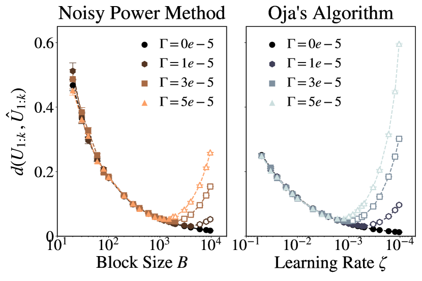
(a) Distance between true column space of $\mathbf{A}_{T}$(; $\mathbf{U}_{1:k}$) and estimated space at $t\!=\!T$(; $\hat{\mathbf{U}}_{1:k}$) as $\Gamma$ varies.

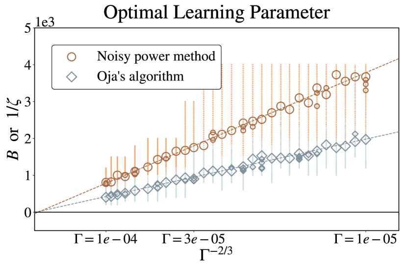
(b) Empirical optimal block size $B$ and learning rate $\zeta$ as $\Gamma$ varies.

Figure 1: Numerical results with synthesized streams of vectors. We used the setting $(\sigma,\delta,p,k)\!=\!(0.15,1.0,100,5)$.

Our first observation in Figure 1(a) is that convergence error decreases as the block size increases without any covariance perturbation ($\Gamma\!=\!0$). This behavior is expected since increasing the number of past information results in better accuracy guarantees for the recovered space in the absence of a covariance shift. However, if the covariance perturbation exists ($\Gamma\!>\!0$), the optimal learning parameter exists, and we have the smaller optimal block size with stronger perturbation. This phenomenon is also expected since an increase in the adversarial budget implies that the past information becomes less relevant. Our observations also corroborate our theoretical results in Theorem 1.

In Figure 1(b), we focus on the optimal value of the block size $B$ and the inverse of the learning rate $1/\zeta$ and its variation with the perturbation budget $\Gamma$. We plot the empirically optimal learning rate for the case of the noisy power method and Oja’s algorithm with $\Gamma^{-2/3}$. We observe that the optimal block size and the inverse learning rate are proportional to $\Gamma^{-2/3}$. This experimental dependency of $\Gamma^{-2/3}$ verifies the theoretically prescribed results in Theorem 2 and 3.

6.1 Experiments on Stock Price Dataset

We provide the real-world benchmark using the S&P500 stock market dataset [44] in Kaggle to test our findings in the non-stationary environment. Refer the Appendix J for the non-stationarity of environments and further experimental details that do not appear in the main paper.

The stream of vectors consisted of 133($=\!p$) companies’ normalized daily returns. Since each company in S&P500 has a different time horizon of available information, we considered 133 companies with the cost information from Mar.18, 1980, to Jul.22, 2022 ($T\!=\!10677$). Then we calculated the ‘daily return,’ which is the difference of adjusted close cost between two days; normalized by the adjusted close cost of the day. The stream of vectors from the environment can be seen as sampled from time-varying distributions with $\Gamma\simeq 0.17$.

The objective is to predict the principal components of the covariance matrix of daily returns as in [61, 4, 54]. We tested the noisy power method and Oja’s algorithm on the preprocessed stream. For the target space $\mathbf{A}_{T}$, we used the $k$-dimensional subspace consisting of top-k singular vectors of covariance estimator calculated with the final 500 samples ($k\!=\!1,\ldots,5$).

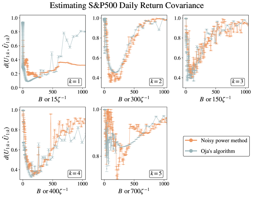
Figure 2: S&P500 stock market daily return prediction, for $k=1,2,\ldots,5$.

The results in Figure 2 indicate that our findings are also valid in the real-world environment with covariance shifts. First, each result shows optimal parameters regimes observed at the U-shaped curves on recovery errors. Furthermore, the result on the noisy power method with varying block size $B$ is akin to the recovery error on Oja’s algorithm, plotted with scaled inverse learning rate $\zeta^{-1}$. These two observations support the main findings in Figure 1(a). We also note that different scaling for each k is natural since we have different spectral gaps $\delta$ between $k$-th and $k\!+\!1$-th spectrums.

7 Conclusion

On the streaming PCA settings with time-varying covariance, we analyzed the fundamental lower bound of the minimax error and estimation errors for the noisy power method and Oja’s algorithm. Under this framework, when no perturbation exists ($\Gamma\!=\!0$), our theoretical result on a lower limit coincides with the order of the traditional outcome. Furthermore, when perturbation exists ($\Gamma\!>\!0$), we have a non-avoidable positive minimax recovery error, although the time horizon becomes arbitrarily long. Next, we found that the noisy power method order-wisely achieves this recovery error and becomes rate-optimal if the $\sigma^{2}\!=\!\Omega(k\delta/p)$. For the optimal learning parameters $B$ or $\zeta^{-1}$, we showed that optimal block size and inverse learning rate minimizing recovery error are similar up to a multiplicative factor and proportional to $\Gamma^{-3/2}$. Experimental results both on the synthetic data and real-world environments support the theoretical findings on the learning parameters.

Although our analysis requires the spectral gap assumption, a recent line of literature considers effective rank [12, 50] as a crucial metric. Therefore, establishing guarantees for robust streaming PCA in terms of effective rank is a perfect direction for future work.

Checklist

The checklist follows the references. Please read the checklist guidelines carefully for information on how to answer these questions. For each question, change the default [TODO] to [Yes] , [No] , or [N/A] . You are strongly encouraged to include a justification to your answer, either by referencing the appropriate section of your paper or providing a brief inline description. For example:

• Did you include the license to the code and datasets? [Yes] The datasets are public datasets and the code is MIT license

Please do not modify the questions and only use the provided macros for your answers. Note that the Checklist section does not count towards the page limit. In your paper, please delete this instructions block and only keep the Checklist section heading above along with the questions/answers below.

1. For all authors…

   1. Do the main claims made in the abstract and introduction accurately reflect the paper’s contributions and scope? [Yes] We explain our new framework and contributions in both abstract and introduction.

   2. Did you describe the limitations of your work? [Yes] There is a result which is partially suboptimal compare to the edge works. We also describe and study the reason for that.

   3. Did you discuss any potential negative societal impacts of your work? [N/A]

   4. Have you read the ethics review guidelines and ensured that your paper conforms to them? [Yes]

2. If you are including theoretical results…

   1. Did you state the full set of assumptions of all theoretical results? [Yes] We provide our assumptions on the Section 3 and Assumption 1

   2. Did you include complete proofs of all theoretical results? [Yes] Detailed Proofs are in the appendix.

3. If you ran experiments…

   1. Did you include the code, data, and instructions needed to reproduce the main experimental results (either in the supplemental material or as a URL)? [Yes] Those are included in the supplemental material.

   2. Did you specify all the training details (e.g., data splits, hyperparameters, how they were chosen)? [Yes] Those are included in the Appendix.

   3. Did you report error bars (e.g., with respect to the random seed after running experiments multiple times)? [Yes] Yes, we repeated every experiment 10 times and reported error bars or uncertainty markers.

   4. Did you include the total amount of compute and the type of resources used (e.g., type of GPUs, internal cluster, or cloud provider)? [Yes] Those are included in the Appendix.

   1. If your work uses existing assets, did you cite the creators? [N/A]

   2. Did you mention the license of the assets? [N/A]

   3. Did you include any new assets either in the supplemental material or as a URL? [N/A]

   4. Did you discuss whether and how consent was obtained from people whose data you’re using/curating? [N/A]

   5. Did you discuss whether the data you are using/curating contains personally identifiable information or offensive content? [N/A] We only used synthesized random matrix data.

4. If you used crowdsourcing or conducted research with human subjects…

   1. Did you include the full text of instructions given to participants and screenshots, if applicable? [N/A]

   2. Did you describe any potential participant risks, with links to Institutional Review Board (IRB) approvals, if applicable? [N/A]

   3. Did you include the estimated hourly wage paid to participants and the total amount spent on participant compensation? [N/A]

Appendix A Discussion on the Cumulative Metric

As discussed on the Section 3, we use $d(\mathrm{ran}(\mathbf{A}_{T}),\phi_{\mathcal{X}})$ as the performance metric. We can make results with respect to the cumulative error $\sum_{t=1}^{T}\mathrm{coeff}^{T-t}\mathrm{metric}(\mathbf{A}_{t},\phi_{\mathcal{X}})$ ($\mathrm{coeff}\in(0,1]$) or $\sum_{t=1}^{T}\mathrm{metric}(\mathbf{A}_{t},\phi_{\mathcal{X}})/T$ from our results of $d(\mathbf{A}_{T},\phi_{\mathcal{X}})$. Note that the distance between actual and estimated space (check the Figure 3(b) for visualization) does not tend to $0$ as $T\to\infty$ on both algorithms when $\Gamma\!>\!0$, which is inevitable as the non-zero lower bound of the Theorem 1 suggests.

To extend our results to the cumulative metric, for the Theorem 1, we can construct a new $\mathcal{A}_{1},\ldots\mathcal{A}_{M^{\prime}}$ for estimating the fundamental lower bound; and for the Theorem 2 and the Theorem 3, our discussion can easily be applied to each $t\in[T]$ (not only to the termination time $T$) using the union bound. However, we have to multiply $\log T$ to the result of $d(\mathbf{A}_{T},\phi_{\mathcal{X}})$ since we use the union bound to have bounded noise matrices from column blocks and the number of blocks linearly increases to $T$. Therefore, when $T\to\infty$, our results become the trivial bound $\sum_{t=1}^{T}\mathrm{metric}(\mathbf{A}_{t},\phi_{\mathcal{X}})/T\leq 1$.

Appendix B Rate Optimality

Our Assumption 1 at the Section 5 allows us to write the clear statement on the performance of two algorithms. Furthermore, by simply truncating the multivariate Gaussian distribution of $\mathbf{x}_{t}$ ($\forall t$) with high probability $1\!-\!1/T$ (we denote this event as $\mathfrak{E}$), we may adopt Assumption 1 on the model with equation (1), for suitable $\mathcal{M}$ and $\mathcal{V}$.

Here we will discuss about the construction of $\mathfrak{E}$, $\mathcal{M}$, and $\mathcal{V}$. To apply the Assumption 1 on the Gaussian model, we define the high-probability($\geq 1\!-\!1/T$) event $\mathfrak{E}$ under $\mathbf{x}_{t}\sim\mathcal{N}(\mathbf{0},\mathbf{\mathbf{A}}_{t}\mathbf{\mathbf{A}}^{\top}_{t}+\sigma^{2}\mathbf{I}_{p\times p})$, where $(\mathbf{A}_{t})_{t=1}^{T}\in\textup{Tu}(\delta,\Gamma)$. Precisely, we define the event $\mathfrak{E}$ at the main paper as below:

Definition 4. Formal Version.

Let $\mathbf{x}_{t}\sim\mathcal{N}(\mathbf{0},\mathbf{\mathbf{A}}_{t}\mathbf{\mathbf{A}}^{\top}_{t}+\sigma^{2}\mathbf{I}_{p\times p})$ and $\mathrm{SVD}(\mathbf{\mathbf{A}}_{t}\mathbf{\mathbf{A}}^{\top}_{t}+\sigma^{2}\mathbf{I}_{p\times p})=\mathbf{U}_{t}\mathbf{D}_{t}\mathbf{U}_{t}^{\top}$. We define the event $\mathfrak{E}$ as follows:

$$\mathfrak{E}:=\>\forall t\in[T]\>:\>\mathbf{z}_{t}=\mathbf{D}_{t}^{-1/2}\mathbf{U}_{t}^{\top}\mathbf{x}_{t}\in[-\rho,\rho]^{\,p}\>\>,\>\>\mathrm{for}\quad\rho=\sqrt{2\log(2pT^{2})}\,.$$

Under the event $\mathfrak{E}$, $\|\mathbf{z}_{t}\|^{2}$ is bounded by $p\rho^{2}=\tilde{\Theta}(p)$. Furthermore, by well-known formula on the variance of truncated normal distribution [13], we have $\mathbb{E}[\mathbf{\mathbf{z}}_{t}\mathbf{\mathbf{z}}^{\top}_{t}|\mathfrak{E}]=(1-\nu(pT^{2}))\mathbf{I}_{p\times p}$ and $\mathbb{E}[\mathbf{\mathbf{x}}_{t}\mathbf{\mathbf{x}}^{\top}_{t}|\mathfrak{E}]=(1-\nu(pT^{2}))\mathbb{E}[\mathbf{\mathbf{x}}_{t}\mathbf{\mathbf{x}}^{\top}_{t}]$ where:

$$\nu(x):=\frac{1}{2\sqrt{\pi}}\frac{\sqrt{\log(x/2)}}{x-1}+\frac{1}{2\pi}\frac{x^{2}}{(x-1)^{4}}\,,$$ (13)

because $\mathbf{z}_{t}\sim\mathcal{N}(\mathbf{0},\mathbf{I}_{p\times p})$. Since $\nu(x)=\mathcal{O}(x^{-1}\log(x/2))$ for $x\gg 1$, we have:

$$\nu(pT^{2})=\mathcal{O}\left(\frac{\log(pT^{2})}{pT^{2}}\right).$$

B.1 Properties under $\mathfrak{E}$

Under the truncation event $\mathfrak{E}$, the expectation of the covariance estimator becomes different. Therefore, the properties which affect to the convergence are also differed, but those are not significant for the sufficiently large $T$. We first define:

$$\mathbf{A}^{\mathfrak{E}}_{t}:=\sqrt{1-\nu(pT^{2})}\mathbf{A}_{t}=\sqrt{1-\mathcal{O}\left(\frac{\log(pT^{2})}{pT^{2}}\right)}\mathbf{A}_{t}\,.$$

Let us first define new parameters as:

$$\{(\sigma^{\mathfrak{E}})^{2},\delta^{\mathfrak{E}},\tilde{\delta}^{\mathfrak{E}},\Gamma^{\mathfrak{E}}\}=(1-\nu(pT^{2}))\{\sigma^{2},\delta,\tilde{\delta},\Gamma\}$$

Then, since $\mathbb{E}[\mathbf{\mathbf{x}}_{t}\mathbf{\mathbf{x}}^{\top}_{t}|\mathfrak{E}]=(1-\nu(pT^{2}))(\mathbf{\mathbf{A}}_{t}\mathbf{\mathbf{A}}^{\top}_{t}+\sigma^{2}\mathbf{I}_{p\times p})=\mathbf{A}^{\mathfrak{E}}_{t}(\mathbf{A}^{\mathfrak{E}}_{t})^{\top}+(\sigma^{\mathfrak{E}})^{2}\mathbf{I}_{p\times p}$, noise magnitude ($\sigma^{2}$), spectral gap of $\mathbf{\mathbf{A}}_{t}\mathbf{\mathbf{A}}^{\top}_{t}$ ($\delta$), largest spectrum of $\mathbf{\mathbf{A}}_{t}\mathbf{\mathbf{A}}^{\top}_{t}$ ($\tilde{\delta}$), and distance between covariance matrix ($\Gamma$) should be replaced by $(1-\nu(pT^{2}))$-scaled new parameters. However, if $T$ is sufficiently large, we restore the original parameters with logarithmic multiplicative factor.

B.2 Applying Assumption 1 under $\mathfrak{E}$

In this section, we will show that under the event $\mathfrak{E}$, the equation (1) satisfies the Assumption 1 (for probability greater than $1-1/T$), with parameters:

1. $\mathcal{M}=(p\tilde{\delta}+k\sigma^{2})\rho^{2}+\tilde{\delta}^{\mathfrak{E}}+(\sigma^{\mathfrak{E}})^{2}$,

2. $\mathcal{V}=(\tilde{\delta}^{\mathfrak{E}}+(\sigma^{\mathfrak{E}})^{2})\mathcal{M}$ .

For the first statement, under $\mathfrak{E}$ we have:

$$\|\mathbf{\mathbf{x}}_{t}\mathbf{\mathbf{x}}^{\top}_{t}-\mathbb{E}[\mathbf{\mathbf{x}}_{t}\mathbf{\mathbf{x}}^{\top}_{t}|\mathfrak{E}]\| =\|\mathbf{D}_{t}^{1/2}(\mathbf{\mathbf{z}}_{t}\mathbf{\mathbf{z}}^{\top}_{t}-\mathbb{E}[\mathbf{\mathbf{z}}_{t}\mathbf{\mathbf{z}}^{\top}_{t}|\mathfrak{E}])\mathbf{D}_{t}^{1/2}\|$$

$$\leq\|\mathbf{D}_{t}^{1/2}\mathbf{z}_{t}\|^{2}+\|\mathbf{D}_{t}^{1/2}(1-\gamma(\mathfrak{E}/pT))\mathbf{I}_{p\times p}\mathbf{D}_{t}^{1/2}\|$$

$$\leq(p\tilde{\delta}+k\sigma^{2})(\rho)^{2}+\tilde{\delta}^{\mathfrak{E}}+(\sigma^{\mathfrak{E}})^{2}\,.$$

Finally, for second argument:

$$\|\mathbb{E}[(\mathbf{\mathbf{x}}_{t}\mathbf{\mathbf{x}}^{\top}_{t}- \mathbb{E}[\mathbf{\mathbf{x}}_{t}\mathbf{\mathbf{x}}^{\top}_{t}|\mathfrak{E}])(\mathbf{\mathbf{x}}_{t}\mathbf{\mathbf{x}}^{\top}_{t}-\mathbb{E}[\mathbf{\mathbf{x}}_{t}\mathbf{\mathbf{x}}^{\top}_{t}|\mathfrak{E}])|\mathfrak{E}]\|$$

$$= \|\mathbb{E}[\mathbf{\mathbf{x}}_{t}\mathbf{\mathbf{x}}^{\top}_{t}\mathbf{\mathbf{x}}_{t}\mathbf{\mathbf{x}}^{\top}_{t}-\mathbf{\mathbf{x}}_{t}\mathbf{\mathbf{x}}^{\top}_{t}\mathbb{E}[\mathbf{\mathbf{x}}_{t}\mathbf{\mathbf{x}}^{\top}_{t}|\mathfrak{E}]|\mathfrak{E}]\|$$

$$\leq \|\mathbf{x}_{t}\|^{2}\|\mathbb{E}[\mathbf{\mathbf{x}}_{t}\mathbf{\mathbf{x}}^{\top}_{t}|\mathfrak{E}]\|+\|\mathbb{E}[\mathbf{\mathbf{x}}_{t}\mathbf{\mathbf{x}}^{\top}_{t}|\mathfrak{E}]\|^{2}$$

$$\leq (p\tilde{\delta}+k\sigma^{2})(\rho)^{2}(\tilde{\delta}^{\mathfrak{E}}+(\sigma^{\mathfrak{E}})^{2})+(\tilde{\delta}^{\mathfrak{E}}+(\sigma^{\mathfrak{E}})^{2})^{2}=(\tilde{\delta}^{\mathfrak{E}}+(\sigma^{\mathfrak{E}})^{2})\mathcal{M}\,.$$

B.3 Discussion

The temporal uncertainty set $\textup{Tu}(\delta,\Gamma)$ does not have any information or clue about $\tilde{\delta}$, which is the upper bound for the first singular value of $\mathbf{\mathbf{A}}_{t}\mathbf{\mathbf{A}}^{\top}_{t}$. Therefore, let us assume $\tilde{\delta}\!=\!\Theta(\delta)$. Then we have:

$$\mathcal{M} \leq 2(p\delta+k\sigma^{2})\log(2pT^{2})$$

$$\mathcal{V} \leq 2(\delta+\sigma^{2})(p\delta+k\sigma^{2})\log(2pT^{2})$$

On this case, the first term of the upper bound for the noisy power method becomes:

$$\mathcal{O}\left(\frac{((\delta+\sigma^{2})(p\delta+k\sigma^{2})\Gamma\log(2pT^{2})\log(2pT^{2}))^{1/3}}{\delta}\right),\text{ or }\tilde{\mathcal{O}}\left(\frac{((\delta+\sigma^{2})(p\delta+k\sigma^{2})\Gamma)^{1/3}}{\delta}\right)\,.$$

By similar procedure, we can also find that our guarantee for Oja’s algorithm is sub-optimal.

Appendix C Preparation for Detailed Proofs

C.1 Notation Table

Table 1: Table of Notations throughout the appendix. We omit notations what we already defined at the Section 1.

Parameters related to the environment:
$T$	time horizon length
$k$	number of principal components
$p$	dimension of observation vectors
$\sigma$	magnitude of observation noise
$\mathbf{\mathbf{A}}_{t}\mathbf{\mathbf{A}}^{\top}_{t}+\sigma^{2}\mathbf{I}_{p\times p}$	covariance matrix at the time $t$
$\delta$	lower bound of spectral gap between $k$th and $k+1$th singular value of $\mathbf{\mathbf{A}}_{t}\mathbf{\mathbf{A}}^{\top}_{t}$
$\tilde{\delta}$	upper bound of the largest spectrum of $\mathbf{\mathbf{A}}_{t}\mathbf{\mathbf{A}}^{\top}_{t}$
$\Gamma$	upper bound of the $\|\mathbf{\mathbf{A}}_{t}\mathbf{\mathbf{A}}^{\top}_{t}-\mathbf{\mathbf{A}}_{t+1}\mathbf{\mathbf{A}}^{\top}_{t+1}\|$
Parameter for the algorithms:
$B$	block size for the noisy power method
$\zeta$	learning rate for the Oja’s algorithm
$\zeta_{\mathrm{opt}}\,,B_{\mathrm{opt}}$	optimal learning parameter when there exists covariance shifts ($\textup{Tu}(\delta,\Gamma)$)
$L(\simeq T/B)$	number of iteration in the noisy power method / for the Oja’s algorithm, $B$ is always the virtual block size corresponding to the optimal parameter $\zeta_{\mathrm{opt}}$
Related to the rate optimality (Section B):
$\mathfrak{E}$	high-probability event under the spiked covariance model setting ($\mathbb{P}[\mathfrak{E}]\geq 1-1/T$), for bounding the norm of observation vectors
$\delta^{\mathfrak{E}}\,,\sigma^{\mathfrak{E}}\,,\Gamma^{\mathfrak{E}},,\tilde{\delta}^{\mathfrak{E}}$	corresponding parameters when we assume the event $\mathfrak{E}$ (since we have different expectation for $\mathbf{\mathbf{x}}_{t}\mathbf{\mathbf{x}}^{\top}_{t}$ under the $\mathfrak{E}$)
$\mathcal{M}\,,\mathcal{V}$	probabilistic upper bound, which plays the role of $\mathcal{M}$ and $\mathcal{V}$ on the spiked covariance model setting
Related to the proof of Theorem 1 (Section D):
${\mathrm{St}}_{k}(\mathbb{R}^{p})$	Stiefel manifold, which consists with the matrix $\mathbf{M}\in\mathbb{R}^{p\times k}$ satisfying $\mathbf{M}^{\top}\mathbf{M}=\mathbf{I}_{k\times k}$
$\mathcal{G}_{k}(\mathbb{R}^{p})$	Grassmann manifold, which is the Riemannian manifold with $k$-dimensional subspace in the $\mathbb{R}^{p}$
$[\mathbf{M}]\in\mathcal{G}_{k}(\mathbb{R}^{p})$	$k$-dimensional subspace generated with the columns of $\mathbf{M}\in{\mathrm{St}}_{k}(\mathbb{R}^{p})$
$\mathcal{G}_{[\mathbf{M}]\rightarrow[\mathbf{N}]}(\Psi^{\prime})$	principal rotation from $[\mathbf{M}]$ to $[\mathbf{N}]$
$s$	latent value for the lower bound

C.2 Technical Lemmas

Lemma 3 (Theorem 2.6.1, [28]).

Let $\mathcal{S}_{1}$ and $\mathcal{S}_{2}$ be two subspaces of $\mathbb{R}^{p}$, such that $\mathrm{dim}(\mathcal{S}_{1})$=$\mathrm{dim}(\mathcal{S}_{2})$. We define the distance between these two subspaces ($\mathcal{S}_{1}$,$\mathcal{S}_{2}$) by $\|\mathbf{P}_{1}-\mathbf{P}_{2}\|$, where $\mathbf{P}_{i},i=1,2$ is the orthogonal projection onto $\mathcal{S}_{i}\>(i=1,2)$. Moreover, suppose $\mathbf{M}=[\underset{k}{\mathbf{M}_{1}}\ \underset{p-k}{\mathbf{M}_{2}}]$, $\mathbf{N}=[\underset{k}{\mathbf{N}_{1}}\ \underset{p-k}{\mathbf{N}_{2}}]$ are $p\times p$ orthogonal matrices. If $\mathcal{S}_{1}=\mathrm{ran}(\mathbf{M}_{1})$ and $\mathcal{S}_{2}=\mathrm{ran}(\mathbf{N}_{1})$, then:

$$\mathrm{dist}(\mathcal{S}_{1},\mathcal{S}_{2})=\|\mathbf{M}^{\top}_{1}\mathbf{N}_{2}\|=\|\mathbf{M}^{\top}_{2}\mathbf{N}_{1}\|\,.$$

Lemma 4 (Davis-Kahan $\sin(\theta)$ theorem; Theorem VII.3.1, [8]).

For given symmetric matrices $\mathbf{M},\mathbf{N}$ with singular value decomposition $\mathrm{SVD}(\mathbf{M})=\mathbf{U}\mathbf{D}\mathbf{U}$ and $\mathrm{SVD}(\mathbf{M}+\mathbf{N})=\hat{\mathbf{U}}\hat{\mathbf{D}}\hat{\mathbf{U}}$, we have:

$$\|\mathbf{U}_{1:k}\mathbf{U}^{\top}_{1:k}-\mathbf{\hat{U}}_{1:k}\mathbf{\hat{U}}^{\top}_{1:k}\|\leq\frac{\|\mathbf{N}\|}{s_{k}(\mathbf{M})-s_{k+1}(\mathbf{M})+\|\mathbf{N}\|}\,.$$

Lemma 5 (Weyl’s theorem).

For any $\mathbf{M},\mathbf{N}\in\mathbb{R}^{p\times k}$ and $1\leq i\leq\min(p,k)$,

$$s_{i}(\mathbf{M}+\mathbf{N})\leq s_{i}(\mathbf{M})+s_{1}(\mathbf{N})\,.$$

Lemma 6 (Sub-additivity of rank).

For any $\mathbf{M},\mathbf{N}\in\mathbb{R}^{p\times k}$,

$$\mathrm{rk}(\mathbf{M}+\mathbf{N})\leq\mathrm{rk}(\mathbf{M})+\mathrm{rk}(\mathbf{N})\,.$$

C.3 Grassmann Manifold

To effectively handle the $k$-dimensional subspace of Euclidean space, we would like to consider the Grassmann manifold [20, 19, 47, 41, 7].

Definition 4 (Grassmann manifold).

Grassmann manifold $\mathcal{G}_{k}(\mathbb{R}^{p})$ is the $k(p-k)$ dimensional Riemannian manifold with $k$-dimensional subspace in $\mathbb{R}^{p}$ as elements. For example, ${\mathbb{R}\mathbb{P}}^{p-1}$ is topologically isomorphic with Grassmann manifold ${\mathcal{G}_{1}(\mathbb{R}^{p})}$. The elements in $\mathcal{G}_{k}(\mathbb{R}^{p})$ are often expressed as the equivalence class $[\mathbf{M}]$ of $p\times k$ orthogonal matrix ($\mathbf{M}\in{\mathrm{St}}_{k}(\mathbb{R}^{p})$). Here, each class is a collection of orthogonal matrices sharing the same column space. A necessary and sufficient condition for both elements of ${\mathrm{St}}_{k}(\mathbb{R}^{p})$ to have the same column space is that the associated projection matrices are the same. That is,

$$\mathbf{M}_{1}\sim\mathbf{M}_{2}\>(\mathbf{M}_{1},\,\mathbf{M}_{2}\in{\mathrm{St}}_{k}(\mathbb{R}^{p}))\Longleftrightarrow\mathbf{M}_{1}\mathbf{M}_{1}^{\top}=\mathbf{M}_{2}\mathbf{M}_{2}^{\top}\,.$$

Definition 5 (Principal angle).

We can define $\mathbf{k}$ principal angles between two elements in $\mathcal{G}_{k}(\mathbb{R}^{p})$. This is clear generalization of an angle $\in[0,\pi/2]$ between two 1d-lines in $\mathbb{R}^{p}$.

1. Let us assume $[\mathbf{M}]\,,[\mathbf{N}]\in\mathcal{G}_{k}(\mathbb{R}^{p})$ ($\mathbf{M}\,,\mathbf{N}\in{\mathrm{St}}_{k}(\mathbb{R}^{p})$). Then we define the principal angle by the inverse cosine of the diagonal matrix $\mathbf{\Sigma}$ in $\text{SVD}(\mathbf{M}^{\top}\mathbf{N})$ $=\mathbf{U}\mathbf{\Sigma}\mathbf{V}^{\top}$. Therefore, the principal angle can be treated as the $k$-dimensional vector in $[0\,,\pi/2]^{k}$.

2. The principle angle is well defined in terms of the fact that:

   $$\text{for }\mathbf{M}_{1}\,,\mathbf{M}_{2}\,,\mathbf{N}_{1}\,,\mathbf{N}_{2}\in{\mathrm{St}}_{k}(\mathbb{R}^{p})\quad\text{s.t}\quad\mathbf{M}_{1}\sim\mathbf{M}_{2}\>\text{ and }\>\mathbf{N}_{1}\sim\mathbf{N}_{2}\,,$$

   $\mathbf{M}_{1}^{\top}\mathbf{N}_{1}$ and $\mathbf{M}_{2}^{\top}\mathbf{N}_{2}$ have same set of singular values.

3. Generally, we mean the set of angles or $k$ dimensional vector or ${k\times k}$ diagonal matrix when we denote principal angle. Specifically, We denote $\Psi=\cos^{-1}(\mathrm{diag}(\mathbf{\Sigma}))$ as the vector in $\mathbb{R}^{k}$ with the principal angles as elements. On the other hand, when we apply trigonometric function on $\Psi$, we treat the result as a diagonal matrix.

To measure the distance between two elements in $\mathcal{G}_{k}(\mathbb{R}^{p})$, we define the projection 2-distance $d_{2}(\cdot\,,\cdot)$, which is the operator 2-norm between projectors of element in $\mathcal{G}_{k}(\mathbb{R}^{p})$. We summarize about the projection distance as follows.

Definition 6 (Projection 2-distance).

Let $[\mathbf{U}],[\mathbf{V}]\in\mathcal{G}_{k}(\mathbb{R}^{p})$ ($\mathbf{U}\,,\mathbf{V}\in{\mathrm{St}}_{k}(\mathbb{R}^{p})$). Assumte that the principal angles between $[\mathbf{U}]$ and $[\mathbf{V}]$ are $\Psi=(\psi_{i})_{i}\in$ $[0\,,\pi/2]^{k}$. We define the projection 2-distance as:

$$d_{2}([\mathbf{U}]\,,[\mathbf{V}]):=\|\mathbf{U}\mathbf{U}^{\top}-\mathbf{V}\mathbf{V}^{\top}\|=\|\sin{\Psi}\|_{\infty}=\max_{1\leq i\leq k}\sin\psi_{i}\,.$$

Note also that the following equality holds for $\mathbf{U}$ and $\mathbf{V}$ in ${\mathrm{St}}_{k}(\mathbb{R}^{p})$:

$$d_{2}([\mathbf{U}]\,,[\mathbf{V}])=d(\mathbf{U},\mathbf{V})(=d(\text{ran}(\mathbf{U}),\text{ran}(\mathbf{V}))\,.$$

We consider the $r$-ball covering with respect to the projection 2-distance. This result can be derived from the slight variation of the proof on the chordal metric $r$-ball [20] (Precisely, we can get the proof by redefining the integral domain $D_{r}$).

Proposition 1 (Projection 2-distance ball in $\mathcal{G}_{k}(\mathbb{R}^{p})$).

Let us define $\mathcal{B}([\mathbf{M}],r)\in\mathcal{G}_{k}(\mathbb{R}^{p})$($r\in(0,1)$) as the $d_{2}$-ball with radius $r$ and center $[\mathbf{M}]$. Then there exists a measure $\mu$ on $\mathcal{G}_{k}(\mathbb{R}^{p})$ such that $\mu(\mathcal{B}([\mathbf{M}],r))\!=\!\mu(r)$ for all $\mathbf{M}]\in\mathcal{G}_{k}(\mathbb{R}^{p})$ where $\mu(r)$ satisfies:

$$c_{p,k}r^{k(p-k)}\leq\mu(r)\leq\frac{c_{p,k}r^{k(p-k)}}{(1-r^{2})^{k/2}}\,.$$

Here, $c_{p,k}$ is a constant determined with $p$ and $k$.

While the rotation between two vectors is self-explanatory, the rotation between two orthogonal planes is not intuitive. Because we have $\mathbf{k}$ principal angles, we may consider k-dimensional rotation. Let $\Psi=\text{diag}(\psi_{i})_{i=1}^{k}$ be the principal angles between $[\mathbf{M}]$ and $[\mathbf{N}]$ ($\mathbf{M}\,,\mathbf{N}\in{\mathrm{St}}_{k}(\mathbb{R}^{p})$). The following definition defines $\mathcal{G}$-mapping, which faithfully generalize traditional rotation.

Definition 7 (Principal rotation).

Let us assume $[\mathbf{M}]\,,[\mathbf{N}]\in\mathcal{G}_{k}(\mathbb{R}^{p})$. Then, we have $\mathcal{G}$-mapping

$$\mathcal{G}_{[\mathbf{M}]\rightarrow[\mathbf{N}]}\>:\>[0\,,\psi_{1}]\times[0\,,\psi_{2}]\times\cdots\times[0\,,\psi_{k}]\rightarrow\mathcal{G}_{k}(\mathbb{R}^{p})\,,$$

which satisfies:

• $\Psi=(\psi_{i})_{i=1}^{k}$ is principal angle between $[\mathbf{M}]$ and $[\mathbf{N}]$.

• $\mathcal{G}_{[\mathbf{M}]\rightarrow[\mathbf{N}]}(0)=[\mathbf{M}]\,,$ and $\mathcal{G}_{[\mathbf{M}]\rightarrow[\mathbf{N}]}(\Psi)=[\mathbf{N}]$.

• Principal angle between $\mathcal{G}(\Psi^{1})$ and $\mathcal{G}(\Psi^{2})$ is $|\,\Psi^{1}-\Psi^{2}\,|$.

From the last property, for $0\!\preceq\!\Psi^{1}\!=\!(\psi_{i}^{1})_{i=1}^{k},\Psi^{2}\!=\!(\psi_{i}^{2})_{i=1}^{k}\!\preceq\!\Psi$, we have:

• $d_{2}(\mathcal{G}(\Psi^{1})\,,\mathcal{G}(\Psi^{2}))=\max_{1\leq i\leq k}|{\sin(\psi_{i}^{1}-\psi_{i}^{2})}|\,$.

Proof.

Consider the following singular value decomposition:

$$\mathbf{M}^{\top}\mathbf{N}=\mathbf{U}\mathbf{\Sigma}\mathbf{V}^{\top}\Rightarrow(\mathbf{M}\mathbf{U})^{\top}(\mathbf{N}\mathbf{V})=\mathbf{\Sigma}=\cos\Psi\,.\quad(0\preceq\Psi\preceq\pi/2)$$

Note that $\mathbf{M}\mathbf{U}\sim\mathbf{M}\,$, $\mathbf{N}\mathbf{V}\sim\mathbf{N}$. We provide the $\mathcal{G}$-mapping from $[\mathbf{M}]$ to $[\mathbf{N}]$:

$$\mathcal{G}_{[\mathbf{M}]\rightarrow[\mathbf{N}]}(\Psi)=[\,\mathbf{M}\mathbf{U}\cos\Psi^{\prime}+(-\mathbf{M}\mathbf{U}\cot{\Psi}+\mathbf{N}\mathbf{V}\csc{\Psi})\sin\Psi^{\prime}\,]\,.\quad(0\preceq\Psi^{\prime}\preceq\Psi)$$

If $\psi_{i}=\psi_{i}^{\prime}=0$, we treat $\sin{\psi^{\prime}_{i}}\,/\!\sin{\psi_{i}}$ as $1$. Since the first two requirements are obvious, we will show that the above formulation satisfies the third condition. From

$$(\mathbf{M}\mathbf{U}\cos\Psi^{\prime})^{\top}(-\mathbf{M}\mathbf{U}\cot{\Psi}+\mathbf{N}\mathbf{V}\csc{\Psi})\sin\Psi^{\prime}=\cos\Psi^{\prime}(-\cot{\Psi}+\cos{\Psi}\csc{\Psi})\sin\Psi^{\prime}=0\,,$$

and

$$\sin\Psi^{1}(-\mathbf{M}\mathbf{U}\cot{\Psi}+\mathbf{N}\mathbf{V}\csc{\Psi})^{\top}(-\mathbf{M}\mathbf{U}\cot{\Psi}+\mathbf{N}\mathbf{V}\csc{\Psi})\sin\Psi^{2}$$

$$= \sin\Psi^{1}\csc\Psi(-\mathbf{M}\mathbf{U}\cos{\Psi}+\mathbf{N}\mathbf{V})^{\top}(-\mathbf{M}\mathbf{U}\cos{\Psi}+\mathbf{N}\mathbf{V})\csc\Psi\sin\Psi^{2}$$

$$= \sin\Psi^{1}\csc\Psi(\mathbf{I}_{p\times p}-\cos^{2}{\Psi})\csc\Psi\sin\Psi^{2}=\sin\Psi\sin\Psi^{2}\,,$$

we have:

$$\mathcal{G}(\Psi^{1})^{\top}\mathcal{G}(\Psi^{2})=\cos\Psi^{1}\cos\Psi^{2}+\sin\Psi^{1}\sin\Psi^{2}=\cos(\Psi^{1}-\Psi^{2})\,.$$

Therefore, the principal angles between $\mathcal{G}(\Psi^{1})$ and $\mathcal{G}(\Psi^{2})$ are $|\Psi^{1}-\Psi^{2}|$. The last property is immediate from the third. ∎

Appendix D Proof of Theorem 1

D.1 Reduction to finite number of hypotheses

Let us define

$$s:=\sqrt[3]{\frac{\log(3/2)}{2160}}\left(\big{(}\frac{\Gamma}{\delta}\big{)}^{1/3}\big{(}\frac{p\sigma^{2}(\sigma^{2}+\delta)}{\delta^{2}}\big{)}^{1/3}+\frac{1}{\sqrt{T}}\big{(}\frac{p\sigma^{2}(\sigma^{2}+\delta)}{\delta^{2}}\big{)}^{1/2}\right)>0,$$

and assume $s<1/3$, and $p>2k+1$ (Note that we assume $p\gg k$). Then we have:

$$\mathbb{E}_{\mathcal{X}\sim\mathbb{P}_{\mathcal{A}}}\Big{(}d(\text{ran}(\mathbf{A}_{T})\,,\,{\phi}_{\mathcal{X}})\Big{)}\geq s\,\mathbb{P}_{\mathcal{A}}\big{(}d(\text{ran}(\mathbf{A}_{T})\,,\,{\phi}_{\mathcal{X}})\geq s\big{)}\,,$$

and

$$\mathcal{R}^{\ast}=\>\inf_{\phi}\sup_{\mathcal{A}\in\textup{Tu}(\delta,\Gamma)}\mathbb{E}_{\mathcal{X}\sim\mathbb{P}_{\mathcal{A}}}\big{(}d\big{(}\text{ran}(\mathbf{A}_{T})\,,\,{\phi}_{\mathcal{X}})\big{)}\\ \geq\>s\cdot\inf_{\phi}\sup_{\mathcal{A}\in\textup{Tu}(\delta,\Gamma)}\mathbb{P}_{\mathcal{A}}\Big{(}d\big{(}\text{ran}(\mathbf{A}_{T})\,,\,{\phi}_{\mathcal{X}}\big{)}\geq s\Big{)}\,.$$

Since we are considering supremum over sequences in $\textup{Tu}(\delta,\Gamma)$, we immediately have that

$$\inf_{\phi}\sup_{\mathcal{A}\in\textup{Tu}(\delta,\Gamma)}\mathbb{P}_{\mathcal{A}}\big{(}d(\text{ran}(\mathbf{A}_{T})\,,\,{\phi}_{\mathcal{X}})\geq s\big{)}\geq\>\inf_{\phi}\sup_{\mathcal{A}\in\{\mathcal{A}_{0}\,,\ldots\,,\mathcal{A}_{M}\}}\mathbb{P}_{\mathcal{A}}\big{(}d(\text{ran}(\mathbf{A}_{T})\,,\,{\phi}_{\mathcal{X}})\geq s\big{)}\,,$$

where $\left\{\mathcal{A}_{i}=\{\mathbf{A}^{(i)}_{1},\mathbf{A}^{(i)}_{2},\ldots,\mathbf{A}^{(i)}_{T}\}\right\}_{i=1}^{T}$ is an appropriately chosen subset of $\textup{Tu}(\delta,\Gamma)$ of size $(M+1)$ which will be defined with the construction below (Section D.2).

D.2 Constructing $\mathbf{A}_{t}^{({i})}$

On the construction, we construct a set with size $M+1$, $\{\mathcal{A}_{i}\}_{i=0}^{M}\subset\textup{Tu}(\delta,\Gamma)$, where $\mathbf{A}_{t}^{({i})}$ ($\forall t\in[T]$ and $\forall i\in[M]\cup\{0\}$) to satisfy:

$$s_{1}(\mathbf{A}^{(i)}_{t}\mathbf{A}^{(i)\top}_{t})=s_{2}(\mathbf{A}^{(i)}_{t}\mathbf{A}^{(i)\top}_{t})=\cdots=s_{k}(\mathbf{A}^{(i)}_{t}\mathbf{A}^{(i)\top}_{t})=\delta\,.$$

Therefore, for the rest of Section D, we treat $\mathbf{A}_{t}^{({i})}$ as orthogonal matrix in $\mathbb{R}^{p\times k}$ for simplicity. We consider the notation $\mathbf{A}_{t}^{({i})}$ as the element of $\mathcal{G}_{k}(\mathbb{R}^{p})$(; equivalence class of orthogonal matrices) or the particular orthogonal matrix in ${\mathrm{St}}_{k}(\mathbb{R}^{p})$. As the matrices in hypothesis are the $\sqrt{\delta}$-scaled orthogonal matrix, notation overloading does not harm the rigorousness of the proof. In summary, if there is no conflict, we denote $\mathbf{A}_{t}^{({i})}$ as orthogonal matrix, or its equivalent class.

We initialize with:

$$\mathcal{A}_{0}=\{\mathbf{A}^{(0)}_{1},\mathbf{A}^{(0)}_{2},\ldots,\mathbf{A}^{(0)}_{T}\}\,,$$

where $\mathbf{A}^{(0)}_{1}=\mathbf{A}^{(0)}_{2}=\cdots=\mathbf{A}^{(0)}_{T}$ with $\mathbf{A}^{(0)}_{T}$= $\big{(}\mathbf{e}_{1},\mathbf{e}_{2},\ldots,\mathbf{e}_{k}\big{)}\in\mathbb{R}^{p\times k}$.

Using the above terminology, we first identify the orthogonal matrix $\mathbf{A}^{(i)}_{T}$ and then construct other elements of $\mathcal{A}_{i}$ from $\mathbf{A}^{(i)}_{T}$. First, we show that we can define $M\!\sim\!(3/2)^{k(p-k)}$ sequences, to bound projection 2-distance between $\mathbf{A}_{T}^{({i})}$ and $\mathbf{A}_{T}^{({j})}$ in the range $[2s\,,6s]$.

Assume that we have sufficiently small $s<1/3$. We want to construct $\mathbf{A}_{T}^{({i})}\in\mathcal{G}_{k}(\mathbb{R}^{p})$ ($i\in[M]$), where $M\!\sim\!(3/2)^{k(p-k)}$ and :

$$\forall(i,j)\>\text{ s.t. }\>i,j\geq 1\text{ and }i\neq j\>:\>2s\leq d_{2}([\mathbf{A}_{T}^{({i})}]\,,[\mathbf{A}_{T}^{({j})}])\leq 6s\,.$$ (14)

$\Longrightarrow$ Let $\mathbf{A}_{T}^{({i})}$ be the elements in $\mathcal{G}_{k}(\mathbb{R}^{p})$. We define $\mathcal{S}_{c}$ and $\mathcal{S}_{i}$ as follows:

$$\mathcal{S}_{c}=\mathcal{B}(\mathbf{A}_{T}^{({0})}\,,3s)\,,\,\mathcal{S}_{i}=\mathcal{B}(\mathbf{A}_{T}^{({i})}\,,2s)\,,$$

where $\mathcal{B}(x\,,r)$ is a projection 2-norm ball in $\mathcal{G}_{k}(\mathbb{R}^{p})$ with radius $r$. Now, we may choose maximal $M$ which keeps the inequality $M\cdot\mu(\mathcal{B}(2s))\leq\mu(\mathcal{B}(3s))$. By using the Proposition 1 on the Appendix C.3, we have:

$$\frac{\mu(\mathcal{B}(\mathbf{A}_{T}^{({0})},3s))}{\mu(\mathcal{B}(\mathbf{A}_{T}^{({i})},2s))}\geq\left(1-(3s)^{2}\right)^{k/2}(3/2)^{k(p-k)}\geq M=\left(3/2\right)^{k(p-k-1/2)}\,.$$

The last inequality comes from the assumption $s<1/3$. If we fix $\mathbf{A}_{T}^{({0})}\in\mathcal{G}_{k}(\mathbb{R}^{p})$, we can select $\mathbf{A}_{T}^{({1})}$ in $\mathcal{S}_{c}$ and exclude $\mathcal{S}_{1}$ from $\mathcal{S}_{c}$. By repeating this process, we can select at least $M$ $k$-dimensional plane $\mathbf{A}_{T}^{({i})}$ while ensuring that $\mathcal{S}_{c}-\bigcup_{1\leq i\leq M-1}\mathcal{S}_{i}$ is non-empty. From the construction, the condition by the equation (14) is satisfied by the triangle inequality.

For the next step, we construct $\mathbf{A}_{t}^{({i})}$($t<T\,,0<i$) satisfying the following second goal:

Let us assume that we constructed $\mathbf{A}_{T}^{({i})}\in\mathcal{G}_{k}(\mathbb{R}^{p})$ to satisfy equation (14). We want to construct $\mathbf{A}_{t}^{({i})}$ for every $t=1\cdots T$ and $i=1\cdots M$, satisfying:

$$d_{2}([\mathbf{A}_{t-1}^{({i})}]\,,[\mathbf{A}_{t}^{({i})}])\leq\frac{\Gamma}{\delta}\,.$$ (15)

$\Longrightarrow$ Let us define the mapping $\mathcal{G}^{(i)}(\Psi(t))$ $\big{(}0\preceq\Psi(t)\preceq\Psi^{(i)}=(\psi_{j}^{(i)})_{j=1}^{k}\big{)}$ as $\mathcal{G}_{[\mathbf{A}_{T}^{({0})}]\rightarrow[\mathbf{A}_{T}^{({i})}]}$ in the Definition 7 on the Appendix C.3. For $t\in[0,T]$, we define $\mathbf{A}_{t}^{({i})}$ as $\mathcal{G}^{(i)}(\Psi(t))$, where $\Psi(t)=(\psi_{1}(t),\ldots,\psi_{k}(t))$ is:

$$\psi_{j}(t)=\begin{cases}0&t\leq T-\left\lfloor d_{2}([\mathbf{A}_{T}^{({0})}]\,,[\mathbf{A}_{T}^{({i})}])\,\delta/\Gamma\right\rfloor\\ \psi_{j}^{(i)}\max\left(1-(T-t)\frac{\Gamma}{\delta\,d_{2}([\mathbf{A}_{T}^{({0})}]\,,[\mathbf{A}_{T}^{({i})}])}\,,0\right)&t>T-\left\lfloor d_{2}([\mathbf{A}_{T}^{({0})}]\,,[\mathbf{A}_{T}^{({i})}])\,\delta/\Gamma\right\rfloor\,.\end{cases}$$

From the property of principal rotation, for every $t\in[T]$, we have

$$d_{2}([\mathbf{A}_{t-1}^{({i})}]\,,[\mathbf{A}_{t}^{({i})}])\leq\max_{1\leq j\leq k}\left(\frac{\Gamma}{\delta}\frac{\psi_{j}^{(i)}}{d_{2}([\mathbf{A}_{T}^{({0})}]\,,[\mathbf{A}_{T}^{({i})}])}\right)=\frac{\Gamma}{\delta}\,.$$

On the last step, we will bound the distance between different hypotheses at arbitrary $t$ with $6s$ as in the case of $t=T$:

$$d_{2}([\mathbf{A}_{t}^{({i})}]\,,[\mathbf{A}_{t}^{({j})}])\leq 6s\,.$$ (16)

$\Longrightarrow$ Here, we bound the above distance as:

$$d_{2}([\mathbf{A}_{t}^{({i})}]\,,[\mathbf{A}_{t}^{({j})}]) \leq d_{2}([\mathbf{A}_{t}^{({i})}]\,,[\mathbf{A}_{T}^{({i})}])+d_{2}([\mathbf{A}_{t}^{({j})}]\,,[\mathbf{A}_{T}^{({j})}]) \mathbf{A}_{0}^{({i})}=\mathbf{A}_{0}^{({j})}=\mathbf{A}_{T}^{({0})}$$ ()

$$\stackrel{{\scriptstyle(\bigstar)}}{{\leq}}d_{2}([\mathbf{A}_{T}^{({i})}]\,,[\mathbf{A}_{0}^{({i})}])+d_{2}([\mathbf{A}_{T}^{({j})}]\,,[\mathbf{A}_{0}^{({j})}])$$

$$\leq 6s\,,$$

where $(\bigstar)$ follows from the construction on the proof of Goal 2.

D.3 Reduction to error probability

Recall that by the construction of the sequence $\{\mathcal{A}_{i}\}$ (Goal 1), we have:

$$\forall(i,j)\>\text{ s.t. }\>i,j\geq 1\text{ and }i\neq j\>:\>2s\leq d_{2}([\mathbf{A}_{T}^{({i})}]\,,[\mathbf{A}_{T}^{({j})}])\,.$$

Therefore, for any estimation of the top eigenvectors ${\phi}_{\mathcal{X}}$, by triangle inequality, we have that

$$\mathbb{P}_{\mathcal{A}_{j}}\big{[}d\big{(}\text{ran}(\mathbf{A}^{(j)}_{T}),{\phi}_{\mathcal{X}}\big{)}\geq s\big{]}\geq\mathbb{P}_{\mathcal{A}_{j}}\big{(}\xi^{\ast}\neq j\big{)}\,,$$

where $\xi^{\ast}:\mathcal{X}\mapsto\mathcal{A}$ denotes the minimum distance test defined by

$$\xi^{\ast}=\text{argmin}_{1\leq i\leq M}d(\text{ran}(\mathbf{A}^{(i)}_{T}),{\phi}_{\mathcal{X}})\,.$$

The above equations imply that:

$$\mathbb{P}_{\mathcal{A}_{j}}\big{[}d(\text{ran}(\mathbf{A}^{(j)}_{T}),{\phi}_{\mathcal{X}}\big{)}\geq s\big{]}\geq\mathbb{P}_{\mathcal{A}_{j}}\big{(}\xi^{\ast}\neq j\big{)}\geq p_{e,M}\,,$$

where $p_{e,M}=\inf_{\xi}\max_{0\leq j\leq M}\mathbb{P}_{\mathcal{A}_{j}}(\xi\neq j)$ and the infimum is over all possible tests $\xi$. To analyze and bound $p_{e,M}$, we use the following Lemma 7.

Lemma 7 (Theorem 2.5 in [57]).

Assume that $\textup{Tu}(\delta,\Gamma)$ contains elements $\mathcal{A}_{0},\mathcal{A}_{1},\ldots,\mathcal{A}_{M}$ ($M\geq 2$) such that

$$\frac{1}{M}\sum_{j=1}^{M}\mathrm{KL}\big{(}\mathbb{P}_{\mathcal{A}_{j}}\|\mathbb{P}_{\mathcal{A}_{0}}\big{)}\leq\alpha\log M.$$

Then, we have

$$p_{e,M}\geq\frac{\sqrt{M}}{1+\sqrt{M}}\Big{(}1-2\alpha-\sqrt{\frac{2\alpha}{\log M}}\Big{)}.$$

To apply Lemma 7, we first bound $\mathrm{KL}\big{(}\mathbb{P}_{\mathcal{A}_{i}}\|\mathbb{P}_{\mathcal{A}_{j}}\big{)}$ for all $i\neq j$. Since $\mathbf{x}_{1},\dots,\mathbf{x}_{T}$ are independent,

$$\mathrm{KL}\big{(}\mathbb{P}_{\mathcal{A}_{i}}\|\mathbb{P}_{\mathcal{A}_{j}}\big{)}=\sum_{t=1}^{T}\mathrm{KL}\big{(}\mathbf{A}^{(i)}_{t}\|\mathbf{A}^{(j)}_{t}\big{)}\leq\min\Big{\{}T,\,d_{2}(\mathbf{A}_{T}^{({0})}\,,\mathbf{A}_{T}^{({i})})\,\delta/\Gamma\Big{\}}\,\mathrm{KL}\big{(}\mathbf{A}^{(i)}_{T}\|\mathbf{A}^{(j)}_{T}\big{)},$$

where $\mathrm{KL}\big{(}\mathbf{A}^{(i)}_{t}\|\mathbf{A}^{(j)}_{t}\big{)}$ is the KL-divergence between two spiked covariance models defined with $\mathbf{A}^{(i)}_{t}$ and $\mathbf{A}^{(j)}_{t}$. We first study the KL-divergence between models with $\mathbf{A}^{(i)}_{T}$ and $\mathbf{A}^{(j)}_{T}$ as below:

$$\mathrm{KL}\big{(}\mathbf{A}^{(i)}_{T}\|\mathbf{A}^{(j)}_{T}\big{)}$$

$$= \log\Bigg{(}\frac{|\delta\mathbf{A}^{(i)}_{T}\mathbf{A}^{(i)\top}_{T}+\sigma^{2}\mathbf{I}_{p\times p}|}{|\delta\mathbf{A}^{(j)}_{T}\mathbf{A}^{(j)\top}_{T}+\sigma^{2}\mathbf{I}_{p\times p}|}\Bigg{)}-p+\mathrm{tr}\Big{(}(\delta\mathbf{A}^{(i)}_{T}\mathbf{A}^{(i)\top}_{T}+\sigma^{2}\mathbf{I}_{p\times p})^{-1}(\delta\mathbf{A}^{(j)}_{T}\mathbf{A}^{(j)\top}_{T}+\sigma^{2}\mathbf{I}_{p\times p})\Big{)}$$

$$= -p+\mathrm{tr}\Big{(}\frac{1}{\sigma^{2}}\big{(}\mathbf{I}_{p\times p}-\frac{\delta}{(\sigma^{2}+\delta)}\mathbf{A}^{(i)}_{T}\mathbf{A}^{(i)\top}_{T}\big{)}(\sigma^{2}\mathbf{I}_{p\times p}+\delta\mathbf{A}^{(j)}_{T}\mathbf{A}^{(j)\top}_{T})\Big{)}$$

$$= -p+\mathrm{tr}\Big{(}\frac{1}{\sigma^{2}}\big{(}\sigma^{2}\mathbf{I}_{p\times p}+\delta\mathbf{A}^{(j)}_{T}\mathbf{A}^{(j)\top}_{T}-\frac{\delta\sigma^{2}}{(\sigma^{2}+\delta)}\mathbf{A}^{(i)}_{T}\mathbf{A}^{(i)\top}_{T}-\frac{\delta^{2}}{(\sigma^{2}+\delta)}\mathbf{A}^{(i)}_{T}\mathbf{A}^{(i)\top}_{T}\mathbf{A}^{(j)}_{T}\mathbf{A}^{(j)\top}_{T}\big{)}\Big{)}$$

$$= \frac{\delta^{2}}{\sigma^{2}(\sigma^{2}+\delta)}\mathrm{tr}\Big{(}\mathbf{A}^{(i)}_{T}\mathbf{A}^{(i)\top}_{T}(\mathbf{I}_{p\times p}-\mathbf{A}^{(j)}_{T}\mathbf{A}^{(j)\top}_{T})\Big{)}$$

$$= \frac{1}{2}\frac{\delta^{2}}{\sigma^{2}(\sigma^{2}+\delta)}\|\mathbf{U}^{(i)}_{T}\mathbf{U}^{(i)\top}_{T}-\mathbf{U}^{(j)}_{T}\mathbf{U}^{(j)\top}_{T}\|_{\text{F}}^{2}\stackrel{{\scriptstyle(\bigstar)}}{{\leq}}\frac{\delta^{2}}{\sigma^{2}(\sigma^{2}+\delta)}k\|\mathbf{U}^{(i)}_{T}\mathbf{U}^{(i)\top}_{T}-\mathbf{U}^{(j)}_{T}\mathbf{U}^{(j)\top}_{T}\|^{2}$$

$$\leq \frac{k\delta^{2}}{\sigma^{2}(\sigma^{2}+\delta)}(6s)^{2}.$$

The $(\bigstar)$ follows from the subadditivity of rank(Lemma 6) and the relation between two norms($\|\mathbf{M}\|_{\textup{F}}\leq\sqrt{\textup{rk}(\mathbf{M})}\|\mathbf{M}\|$). Therefore, we have the following upper bound:

$$\mathrm{KL}\big{(}\mathbb{P}_{\mathcal{A}_{i}}\|\mathbb{P}_{\mathcal{A}_{j}}\big{)} \leq\frac{36k\delta^{2}}{\sigma^{2}(\sigma^{2}+\delta)}\min\Big{\{}T,\,d_{2}(\mathbf{A}_{T}^{({0})}\,,\mathbf{A}_{T}^{({i})})\,\delta/\Gamma\Big{\}}s^{2}$$

$$\leq\frac{36k\delta^{2}}{\sigma^{2}(\sigma^{2}+\delta)}\min\Big{\{}T,\,\frac{3s\delta}{\Gamma}\Big{\}}s^{2}\,,$$ (17)

where the last inequality comes from the construction of Goal 1.

D.4 Proving the Theorem

Now, we establish Theorem 1 based on the progress so far. As mentioned at the last section, we are using the notation $\mathbf{A}_{t}^{({i})}$ to represent an orthogonal matrix(or its class), not scaled with $\sqrt{\delta}$. We first start from the result in the Appendix D.1:

$$1/3>\forall s>0\>:\>\mathcal{R}^{*}\geq s\inf_{\phi}\sup_{\mathcal{A}\in\{\mathcal{A}_{i}\}_{i=0}^{M}}\mathbb{P}_{\mathcal{A}}\left[d(\mathrm{ran}(\mathbf{A}_{T})\,,\phi_{\mathcal{X}})\geq s\right]\,,$$

where $d_{2}(\cdot\,,\cdot)$ is distance defined by operator norm between projectors. From the construction of Goal 1$\sim$3 on the Appendix D.2, we bound the KL divergence between hypothesis at the equation (17):

$$\mathrm{KL}\big{(}\mathbb{P}_{\mathcal{A}_{i}}\|\mathbb{P}_{\mathcal{A}_{j}}\big{)}\leq\frac{36k\delta^{2}}{\sigma^{2}(\sigma^{2}+\delta)}\min\Big{\{}T,\,\frac{3s\delta}{\Gamma}\Big{\}}s^{2}\,.$$

Now, we find the particular range of $s$ satisfying:

$$\mathrm{KL}(\mathbb{P}_{\mathcal{A}_{i}}\|\mathbb{P}_{\mathcal{A}_{j}})\leq\frac{36\delta^{2}}{\sigma^{2}(\sigma^{2}+\delta)}k\min\left(T,\frac{3\delta}{\Gamma}\,s\right)s^{2}\stackrel{{\scriptstyle(\bigstar 1)}}{{\leq}}\frac{1}{10}\log{M}=\frac{1}{10}\log\left(\left(3/2\right)^{k(p-k-1/2)}\right)\,.$$

Note that ($\bigstar 1$) is satisfied when the ($\bigstar 2$) of the following inequality holds:

$$\frac{360\delta^{2}}{\sigma^{2}(\sigma^{2}+\delta)}\min\left(T,\frac{3\delta}{\Gamma}\,s\right)s^{2}\stackrel{{\scriptstyle(\bigstar 2)}}{{\leq}}\frac{1}{2}p\log{\frac{3}{2}}\leq(p-k-\frac{1}{2})\log{\frac{3}{2}}\,.$$

Therefore, we have a constant $({\log(3/2)/2160})^{1/3}\simeq 0.05726>0$ such that with

$$s=\sqrt[3]{\frac{\log(3/2)}{2160}}\left(\big{(}\frac{\Gamma}{\delta}\big{)}^{1/3}\big{(}\frac{p\sigma^{2}(\sigma^{2}+\delta)}{\delta^{2}}\big{)}^{1/3}+\frac{1}{\sqrt{T}}\big{(}\frac{p\sigma^{2}(\sigma^{2}+\delta)}{\delta^{2}}\big{)}^{1/2}\right)\,,$$ (18)

we have

$$\frac{1}{M}\sum_{j=1}^{M}\mathrm{KL}(\mathbb{P}_{\mathcal{A}_{j}}\|\mathbb{P}_{\mathcal{A}_{0}})\leq\frac{1}{10}\log{M}\,.$$

Finally, we use the reduction to error probability argument at the Appendix D.1. For $p_{e,M}=\inf_{\xi}\max_{0\leq j\leq M}\mathbb{P}_{\mathcal{A}_{j}}(\xi\neq j)$,

$$\mathbb{P}_{\mathcal{A}_{j}}\left[d(\mathrm{ran}(\mathbf{A}_{T})\,,\phi_{\mathcal{X}})\geq s\right]\geq\mathbb{P}_{\mathcal{A}_{j}}(\xi\neq j)\geq p_{e,M}\,.$$

Now, with $s$ in the equation (18), we have the following:

$$\mathcal{R}^{*} \geq s\cdot\inf_{\phi}\sup_{\mathcal{A}\in\{\mathcal{A}_{0}\,,\mathcal{A}_{1}\,,\ldots,\mathcal{A}_{M}\}}\mathbb{P}_{\mathcal{A}}\left[d(\mathrm{ran}(\mathbf{A}_{T})\,,\phi_{\mathcal{X}})\geq s\right]$$

$$\geq s\cdot p_{e,M}=\sqrt[3]{\frac{\log(3/2)}{2160}}\left(\big{(}\frac{\Gamma}{\delta}\big{)}^{1/3}\big{(}\frac{p\sigma^{2}(\sigma^{2}+\delta)}{\delta^{2}}\big{)}^{1/3}+\frac{1}{\sqrt{T}}\big{(}\frac{p\sigma^{2}(\sigma^{2}+\delta)}{\delta^{2}}\big{)}^{1/2}\right)p_{e,M}\,,$$

where the $p_{e,M}$ is lower bounded by $\sim 0.8$ since $M\geq 1.5^{pk/2}$ is sufficiently large . $\blacksquare$

Appendix E Proof of Lemma 1

We prove the Lemma 1 under the condition $\mathbb{E}[\mathbf{\mathbf{x}}_{t}\mathbf{\mathbf{x}}^{\top}_{t}]=\mathbf{\mathbf{A}}_{t}\mathbf{\mathbf{A}}^{\top}_{t}+\sigma^{2}\mathbf{I}_{p\times p}$ and Assumption 1 defined at the Section 5 holds. Later at the Appendix B, we apply this result on the our original model. We first start from the decomposition of $\frac{1}{B}\sum_{t=(\ell-1)B+1}^{\ell B}\mathbf{x}_{t}\mathbf{x}^{\top}_{t}$,

$$\frac{1}{B}\sum_{t=(\ell-1)B+1}^{\ell B}\mathbf{\mathbf{x}}_{t}\mathbf{\mathbf{x}}^{\top}_{t}=\mathbb{E}[\mathbf{\mathbf{x}}_{\ell B}\mathbf{\mathbf{x}}^{\top}_{\ell B}]+\mathbf{\mathcal{E}}(\ell)=\mathbf{\mathbf{A}}_{\ell B}\mathbf{\mathbf{A}}^{\top}_{\ell B}+\sigma^{2}\mathbf{I}_{p\times p}+\mathcal{E}(\ell)=\mathbf{M}(\ell)+\mathcal{E}(\ell)\,.$$

Note that formulation for $\mathcal{E}(\ell)$ is following:

$$\mathcal{E}(\ell)=\frac{1}{B}\mkern-20.0mu\sum_{t=(\ell-1)B+1}^{\ell B}\mkern-20.0mu\mathbf{\mathbf{x}}_{t}\mathbf{\mathbf{x}}^{\top}_{t}-\mathbb{E}[\mathbf{\mathbf{x}}_{\ell B}\mathbf{\mathbf{x}}^{\top}_{\ell B}]\,.$$

We would decompose $\mathcal{E}(\ell)$ in two terms as following.

$$\mathcal{E}(\ell) =\frac{1}{B}\mkern-12.0mu\sum_{t=(\ell-1)B+1}^{\ell B}\Big{(}\mathbf{\mathbf{x}}_{t}\mathbf{\mathbf{x}}^{\top}_{t}-\mathbb{E}[\mathbf{\mathbf{x}}_{t}\mathbf{\mathbf{x}}^{\top}_{t}]+\mathbb{E}[\mathbf{\mathbf{x}}_{t}\mathbf{\mathbf{x}}^{\top}_{t}]-\mathbb{E}[\mathbf{\mathbf{x}}_{\ell B}\mathbf{\mathbf{x}}^{\top}_{\ell B}]\Big{)}$$

$$=\underbrace{\frac{1}{B}\sum_{t=(\ell-1)B+1}^{\ell B}\Big{(}\mathbf{\mathbf{x}}_{t}\mathbf{\mathbf{x}}^{\top}_{t}-\mathbb{E}[\mathbf{x}_{t}\mathbf{x}_{t}]\Big{)}}_{\mathcal{E}_{1}(\ell)}+\,\underbrace{\frac{1}{B}\sum_{t=(\ell-1)B+1}^{\ell B}\Big{(}\mathbb{E}[\mathbf{\mathbf{x}}_{t}\mathbf{\mathbf{x}}^{\top}_{t}]-\mathbb{E}[\mathbf{\mathbf{x}}_{\ell B}\mathbf{\mathbf{x}}^{\top}_{\ell B}]\Big{)}}_{\mathcal{E}_{2}(\ell)}\,.$$

E.1 Bounding $\max_{\ell}{\lVert\mathcal{E}_{1}(\ell)\rVert}$ with probability $1-1/T$

First, we bound the $\mathcal{E}_{1}(\ell)$ using the following matrix Bernstein inequality.

Theorem 4 (Matrix Bernstein Inequality [56]).

Let $\mathbf{X}_{1}\,,\ldots,\mathbf{X}_{B}\in\mathbb{R}^{p\times p}$ be independent, centered, symmetric real random variables, and assume that each one is uniformly bounded:

$$\mathbb{E}[\mathbf{X}_{i}]=\mathbf{0}\>\>\text{ and }\>\>\lVert\mathbf{X}_{i}\rVert\leq\mathcal{M}\quad\text{for each }i=1\,,\ldots,B\,.$$

and let $\mathcal{V}$ denote upper bound for the matrix variance statistics of the sum:

$$\mathcal{V}\geq\lVert\mathbb{E}[\mathbf{X}_{i}^{2}]\rVert\,.$$

Then

$$\mathbb{P}\left\{\Big{\|}\frac{1}{B}\sum_{i=1}^{B}\mathbf{X}_{i}\Big{\|}\geq x\right\}\leq 2p\exp\left\{\frac{-Bx^{2}}{2(\mathcal{V}+\mathcal{M}x/3)}\right\}\,.$$

We set $\mathbf{X}_{t}$ as $\mathbf{x}_{t}\mathbf{x}^{\top}_{t}-\mathbb{E}[\mathbf{x}_{t}\mathbf{x}^{\top}_{t}]$ for all $(\ell-1)B+1\leq t\leq\ell B$ and overload the notation $\mathcal{M}$ and $\mathcal{V}$. Consider the following inequality:

$$\log(2pT^{2})\leq\frac{Bx^{2}}{2(\mathcal{V}+\mathcal{M}x/3)}\,.$$

Then we have following sufficient condition for the above inequality:

$$x\geq\frac{\mathcal{M}\log(2pT^{2})}{3B}\left[1+\sqrt{1+\frac{18\mathcal{V}}{\mathcal{M}^{2}}\frac{B}{\log{2pT^{2}}}}\right]\,.$$

From the inequality $\sqrt{1+x}\leq 1+\sqrt{x}(x\geq 0)$, we get the following argument.

$$\text{If}\>\>x=\frac{\mathcal{M}}{3}\frac{\log{2pT^{2}}}{B}+\sqrt{2\mathcal{V}}\sqrt{\frac{\log{2pT^{2}}}{B}}\,,\>\>\text{then}\>\>\mathbb{P}\left\{\Big{\|}\frac{1}{B}\mkern-12.0mu\sum_{t=(\ell-1)B+1}^{\ell B}\mathbf{X}_{t}\Big{\|}\geq x\right\}\leq\frac{1}{T^{2}}\,.$$

Let us assume the condition $\mathcal{M}^{2}\log(2pT^{2})/\mathcal{V}\leq B$. Then, with probability greater than $1-1/T^{2}$, we have that:

$$\|\mathcal{E}_{1}(\ell)\|=\Big{\|}\frac{1}{B}\mkern-12.0mu\sum_{t=(\ell-1)B+1}^{\ell B}\mathbf{X}_{t}\Big{\|}\leq\frac{1+3\sqrt{2}}{3}\sqrt{\frac{\mathcal{V}\log(2pT^{2})}{B}}\,.$$

Now, we use the union bound argument. That is, for probability greater than $1-1/T$ ($\leq 1-(T/B)/T^{2}$),

$$\max_{1\leq\ell\leq L(=T/B)}\|\mathcal{E}_{1}(\ell)\|\leq\frac{1+3\sqrt{2}}{3}\sqrt{\frac{\mathcal{V}\log(2pT^{2})}{B}}\,.$$

E.2 Bounding $\lVert\mathcal{E}_{2}(\ell)\rVert$ for all $\ell$

Since the our model limits the perturbation amount of covariance matrix, we may bound the $\lVert\mathcal{E}_{2}(\ell)\rVert$ as follows:

$$\lVert\mathcal{E}_{2}(\ell)\rVert \leq\Big{\lVert}\frac{1}{B}\sum_{t=(\ell-1)B+1}^{\ell B}\Big{(}\mathbb{E}[\mathbf{\mathbf{x}}_{t}\mathbf{\mathbf{x}}^{\top}_{t}]-\mathbb{E}[\mathbf{\mathbf{x}}_{\ell B}\mathbf{\mathbf{x}}^{\top}_{\ell B}]\Big{)}\Big{\rVert}\leq\frac{1}{B}\sum_{t=(\ell-1)B+1}^{\ell B}\lVert\mathbb{E}[\mathbf{\mathbf{x}}_{t}\mathbf{\mathbf{x}}^{\top}_{t}]-\mathbb{E}[\mathbf{\mathbf{x}}_{\ell B}\mathbf{\mathbf{x}}^{\top}_{\ell B}]\rVert$$

$$=\frac{1}{B}\sum_{t=(\ell-1)B+1}^{\ell B}\lVert\mathbf{\mathbf{A}}_{t}\mathbf{\mathbf{A}}^{\top}_{t}-\mathbf{\mathbf{A}}_{\ell B}\mathbf{\mathbf{A}}^{\top}_{\ell B}\rVert\leq\frac{1}{B}\sum_{t=(\ell-1)B+1}^{\ell B}(\ell B-t)\Gamma$$

$$\leq\frac{1}{B}\frac{B(B-1)}{2}\Gamma\leq\frac{B\Gamma}{2}\,.$$

E.3 Bounding ${\lVert\mathcal{E}(\ell)\rVert}$ for all $\ell$, with high probability

On the Appendix E.1, we bounded $\max_{\ell}{\lVert\mathcal{E}_{1}(\ell)\rVert}$ for the probability greater than $1-1/T$. Therefore, for probability greater than $1-1/T$,

$$\max_{\ell}{\lVert\mathcal{E}(\ell)\rVert}\leq\max_{\ell}{\lVert\mathcal{E}_{1}(\ell)\rVert}+\max_{\ell}{\lVert\mathcal{E}_{2}(\ell)\rVert}\leq\frac{1+3\sqrt{2}}{3}\sqrt{\frac{\mathcal{V}\log(2pT^{2})}{B}}+\frac{B\Gamma}{2}\,.$$ (19)

$\blacksquare$

Appendix F Proof of Theorem 2

We prove the Theorem 2 under the condition defined by the equation (19), which holds for probability greater than $1-1/T$.

F.1 Deriving optimal learning block size $B$

Consider the upper bound (for probability greater than $1-1/T$) on $\max_{\ell}{\lVert\mathcal{E}(\ell)\rVert}$ from the Appendix E:

$$\max_{\ell}{\lVert\mathcal{E}(\ell)\rVert}\leq C_{\mathrm{NPM}}\sqrt{\frac{\log{2pT^{2}}}{B}}+\frac{B\Gamma}{2}\,,\text{ where }C_{\mathrm{NPM}}=\frac{1+3\sqrt{2}}{3}\sqrt{\mathcal{V}}\,.$$

By differentiating and find the critical point, we have the following optimal block size:

$$B_{\mathrm{opt}}=\frac{{C_{\mathrm{NPM}}}^{2/3}\log(2pT^{2})^{1/3}}{\Gamma^{2/3}}=\Omega\left(\frac{\mathcal{V}^{2/3}\log(2pT^{2})^{1/3}}{\Gamma^{2/3}}\right)\,.$$

In this case, the uniform upper bound for error matrix becomes:

$$\max_{\ell}{\lVert\mathcal{E}(\ell)\rVert}\leq\frac{3}{2}{C}_{\mathrm{NPM}}^{2/3}\log(2pT^{2})^{1/3}\Gamma^{1/3}\,.$$

F.2 Defining Regime and Parameters

Let us set $B=B_{\mathrm{opt}}$ and consider the regime:

1. $36B_{\mathrm{opt}}\Gamma=24\,{C}_{\mathrm{NPM}}^{2/3}\log(2pT^{2})^{1/3}\Gamma^{1/3}\leq\delta$, from $\Gamma=\mathcal{O}\left(\frac{\delta^{3}}{{C}_{\mathrm{NPM}}^{2}\log(2pT^{2})}\right)\,.$

2. $\delta\geq\frac{12}{17}\sigma^{2}\,.$

For this regime, we define $\Lambda\,,\epsilon\,,\eta>0$ as:

1. $\displaystyle\Lambda:=\frac{3}{2}B_{\mathrm{opt}}\Gamma=\frac{3}{2}{C}_{\mathrm{NPM}}^{2/3}\log(2pT^{2})^{1/3}\Gamma^{1/3}$

   $\,(\geq\max_{\ell}{\lVert\mathcal{E}(\ell)\rVert}\text{ on probability greater than }1-1/T,\text{ shown at the Appendix~{}\ref{derive_npm_optimal_B}})\,.$

2. $\displaystyle\epsilon:=\frac{4\Lambda}{\delta}\leq\frac{1}{4}\,.$

3. $\displaystyle\eta:=\frac{B_{\mathrm{opt}}\Gamma}{\delta-B_{\mathrm{opt}}\Gamma}\,.$

Note that from the item (A) and (c) above, we have:

$$\frac{\eta}{\epsilon}=\frac{B_{\mathrm{opt}}\Gamma/(\delta-B_{\mathrm{opt}}\Gamma)}{4\Lambda/\delta}=\frac{B_{\mathrm{opt}}\Gamma/(\delta-B_{\mathrm{opt}}\Gamma)}{6B_{\mathrm{opt}}\Gamma/\delta}=\frac{1}{6}\frac{\delta}{\delta-B_{\mathrm{opt}}\Gamma}\leq\frac{6}{35}\leq\frac{1}{5}\,.$$

With this parameters, we show the following lemma:

Lemma 8.

Assume the regime in the above. Let $\mathbf{M}\in\mathbb{R}^{n\times n}$ be a positive definite matrix and SVD$(\mathbf{M})=\mathbf{U}\mathbf{D}\mathbf{U}^{\top}$ with $s_{k}(\mathbf{M})\geq\delta+\sigma^{2}$ and $s_{k+1}(\mathbf{M})=\sigma^{2}$. Then we have:

• $\beta:=(1-(\eta+\epsilon)^{2})\frac{\delta+\sigma^{2}-{\Lambda}/{\sqrt{1-(\eta+\epsilon)^{2}}}}{\sigma^{2}+\Lambda}\geq 1.4465>\frac{1}{0.7}>1\,.$

• $\frac{\epsilon}{\sqrt{1-\epsilon^{2}}}\frac{s_{k}(\mathbf{M})-\Lambda/\epsilon}{s_{k+1}(\mathbf{M})+\Lambda/\sqrt{1-\epsilon^{2}}}\geq\frac{\epsilon}{\sqrt{1-\epsilon^{2}}}\frac{0.75s_{k}(\mathbf{M})+0.25s_{k+1}(\mathbf{M})}{0.25s_{k}(\mathbf{M})+0.75s_{k+1}(\mathbf{M})}\stackrel{{\scriptstyle(\spadesuit)}}{{>}}\frac{\epsilon+\eta}{\sqrt{1-(\epsilon+\eta)^{2}}}.$

• $\frac{s_{k}(\mathbf{M})-\Lambda/\sqrt{1-(\epsilon+\eta)^{2}}}{s_{k+1}(\mathbf{M})+\Lambda/(\epsilon+\eta)}\frac{\sqrt{1-(\epsilon+\eta)^{2}}}{\epsilon+\eta}>\frac{\sqrt{1-\epsilon^{2}}}{\epsilon}\,.$

Proof.

Here we provide the bound for $(\epsilon+\eta)$: $\epsilon+\eta\leq 6\epsilon/5\leq 3/10\,.$ For the first item, we have:

$$\beta{\geq}\frac{91}{100}\frac{\delta+\sigma^{2}-\sqrt{100/91}\,{\Lambda}}{\sigma^{2}+\Lambda}{\geq}\frac{91}{100}\frac{\delta+\sigma^{2}-\sqrt{100/91}\,{\delta}/16}{\sigma^{2}+\delta/16}=\frac{91}{100}\frac{\left(1-\sqrt{\frac{100}{91}}\frac{1}{16}\right)+\frac{\sigma^{2}}{\delta}}{\frac{1}{16}+\frac{\sigma^{2}}{\delta}}{\geq}1.4465\,.$$

where the inequalities follows from $\epsilon+\eta\leq 3/10$, $\Lambda\leq\delta/16$, and $\delta\geq 12\sigma^{2}/17$ respectively.

For the second one, the first inequality is immediate from $\epsilon\leq 1/4$. We now show the inequality $(\spadesuit)$. We provide the sufficient condition as:

$$\left(\frac{\epsilon}{\sqrt{1-\epsilon^{2}}}\frac{\sigma^{2}+\frac{3}{4}\delta}{\sigma^{2}+\frac{1}{4}\delta}=\right)\frac{\epsilon}{\sqrt{1-\epsilon^{2}}}\frac{\frac{\sigma^{2}}{\delta}+\frac{3}{4}}{\frac{\sigma^{2}}{\delta}+\frac{1}{4}}\geq\frac{\epsilon+\eta}{\sqrt{1-(\epsilon+\eta)^{2}}}$$

$$\Longleftarrow\quad \left(\frac{\epsilon}{\sqrt{1-\epsilon^{2}}}\frac{17/12+{3}/{4}}{17/12+{1}/{4}}=\right)\frac{13}{10}\frac{\epsilon}{\sqrt{1-\epsilon^{2}}}\geq\frac{\epsilon+\eta}{\sqrt{1-(\epsilon+\eta)^{2}}} (\delta\geq\frac{12\sigma^{2}}{17})$$

$$\Longleftrightarrow\quad 1.69\left(\frac{\epsilon}{\epsilon+\eta}\right)^{2}-1\geq 0.69\epsilon^{2}$$

$$\Longleftarrow\quad 1.69\left(\frac{\epsilon}{\epsilon+\eta}\right)^{2}-1\geq\frac{0.69}{16} (\epsilon\leq 1/4)$$

$$\Longleftarrow\quad \eta\leq 0.288\,\epsilon\,.$$

The final condition is automatically satisfied the inequality $\eta\leq\epsilon/5$ (from the definition of $\eta$). Therefore, we proved the second inequality.

For the last inequality, enough to show:

$$\frac{\epsilon+\eta}{\sqrt{1-(\epsilon+\eta)^{2}}}\frac{\sigma^{2}\>+\>{\delta\epsilon}/{4(\epsilon+\eta)}}{\sigma^{2}+\delta\>-\>{\delta\epsilon}/{4\sqrt{1-(\epsilon+\eta)^{2}}}}\leq\frac{\epsilon}{\sqrt{1-\epsilon^{2}}}\,.$$

We upper bound second term of LHS:

$$\frac{\sigma^{2}\>+\>{\delta\epsilon}/{4(\epsilon+\eta)}}{\sigma^{2}+\delta\>-\>{\delta\epsilon}/{4\sqrt{1-(\epsilon+\eta)^{2}}}} =\frac{\sigma^{2}/\delta\>+\>{\epsilon}\big{/}{4(\epsilon+\eta)}}{\sigma^{2}/\delta+(1\>-\>{\epsilon}\big{/}{4\sqrt{1-(\epsilon+\eta)^{2}}})}$$

$$\stackrel{{\scriptstyle(\blacksquare)}}{{\leq}}\frac{17/12\>+\>{\epsilon}\big{/}{4(\epsilon+\eta)}}{17/12+(1\>-\>{\epsilon}\big{/}{4\sqrt{1-(\epsilon+\eta)^{2}}})}$$

$$\stackrel{{\scriptstyle(\blacklozenge)}}{{\leq}}\frac{17/12\>+\>{\epsilon}\big{/}{4(\epsilon+\eta)}}{29/12\>-\>{\epsilon}\big{/}{4(\epsilon+\eta)}}$$

$$\leq\frac{17/3\>+\>1/{(1+\eta/\epsilon)}}{29/3\>-\>1/{(1+\eta/\epsilon)}}\leq\frac{10}{13}\,,$$

where the $(\blacksquare)$ comes from:

$$\epsilon+\eta\leq\frac{1}{\sqrt{2}}\leq\sqrt{1-(\epsilon+\eta)^{2}}\Longrightarrow\>\> \frac{\epsilon}{4}\left(\frac{1}{\epsilon+\eta}+\frac{1}{\sqrt{1-(\epsilon+\eta)^{2}}}\right)\leq\frac{\epsilon}{4}\frac{2}{\epsilon+\eta}\leq\frac{1}{2}$$

$$\Longrightarrow\>\> \underline{1-\frac{\epsilon}{4\sqrt{1-(\epsilon+\eta)^{2}}}\geq\frac{\epsilon}{4(\epsilon+\eta)}}\,,$$

and the $(\blacklozenge)$ is immediate from $\epsilon+\eta\leq\frac{1}{\sqrt{2}}\leq\sqrt{1-(\epsilon+\eta)^{2}}$. Finally, the only left part is :

$$\frac{10}{13}\frac{\epsilon+\eta}{\sqrt{1-(\epsilon+\eta)^{2}}}\leq\frac{\epsilon}{\sqrt{1-\epsilon^{2}}}\,,$$

which was shown (from $\eta\leq\epsilon/5$), when we proved the inequality ($\spadesuit$) above. ∎

F.3 Lemmas for $\mathbf{N}^{(\ell)}$ and $\mathbf{W}^{(\ell)}$

Lemma 9 (Orthogonal amplification).

Assume the regime in the Appendix F.2. Let $\mathbf{M}\in\mathbb{R}^{p\times p}$ be a positive definite matrix and $\mathrm{SVD}(\mathbf{M})=\mathbf{U}\mathbf{D}\mathbf{U}^{\top}$. Moreover, let $\mathcal{E}\in\mathbb{R}^{p\times p}$ with $\lVert\mathcal{E}\rVert\leq\Lambda$. For $0<k$ $<p$, let $\mathcal{Y}$ be the set of $\mathbf{Y}\in$ ${\mathrm{St}}_{p-k}(\mathbb{R}^{p})$ such that $s_{1}\left(\mathbf{U}_{1:k}^{\top}\mathbf{Y}\right)\leq\epsilon+\eta$. For every given $\mathbf{Y}\in\mathcal{Y}$, there exists a $\overline{\mathbf{N}}\in{\mathrm{St}}_{p-k}(\mathbb{R}^{p})$ such that

$$\mathrm{ran}\left((\mathbf{M}+\mathcal{E})\overline{\mathbf{N}}\right)\subseteq\mathrm{ran}\left(\mathbf{Y}\right),~{}s_{1}\left(\mathbf{U}_{1:k}^{\top}\overline{\mathbf{N}}\right)\leq\epsilon,$$ (20)

$$s_{1}\left((\mathbf{M}+\mathcal{E})\overline{\mathbf{N}}\right)\leq\frac{\sigma^{2}+\Lambda}{\sqrt{1-(\epsilon+\eta)^{2}}}.$$ (21)

Proof.

We first show that for any positive definite matrix $\mathbf{M}\in\mathbb{R}^{p\times p}$, $\mathcal{E}\in\mathbb{R}^{p\times p}$ and $\mathbf{Y}\in\mathcal{Y}$, there exists $\overline{\mathbf{N}}\in{\mathrm{St}}_{p-k}(\mathbb{R}^{p})$ such that $\mathrm{ran}\left((\mathbf{M}+\mathcal{E})\overline{\mathbf{N}}\right)\subseteq\mathrm{ran}\left(\mathbf{Y}\right)$ as follows:

1. When $\mathbf{M}+\mathcal{E}$ is a full-rank matrix, $\mathrm{ran}\left((\mathbf{M}+\mathcal{E})\overline{\mathbf{N}}\right)=\mathrm{ran}\left(\mathbf{Y}\right)$ with $\overline{\mathbf{N}}=b\left((\mathbf{M}+\mathcal{E})^{-1}\mathbf{Y}\right)$.

2. When the rank of $\mathbf{M}+\mathcal{E}$ is $r\leq k$, every $\overline{\mathbf{N}}$ such that $(\mathbf{M}+\mathcal{E})\overline{\mathbf{N}}=\mathbf{0}$ satisfies that $\mathrm{ran}\left((\mathbf{M}+\mathcal{E})\overline{\mathbf{N}}\right)=\emptyset\subseteq\mathrm{ran}\left(\mathbf{Y}\right)$.

3. Assume that the rank of $\mathbf{M}+\mathcal{E}$ is $r,\ k<r<p$. We identify $\overline{\mathbf{N}}$ in parts by identifying the first $(r-k)$ columns and then the remaining columns. Let $(\mathbf{M}+\mathcal{E})=\tilde{\mathbf{U}}\tilde{\mathbf{D}}\tilde{\mathbf{V}}^{\top}$ and $\mathbf{Y}^{\top}\mathbf{\tilde{U}}_{1:r}=\hat{\mathbf{U}}\hat{\mathbf{D}}\hat{\mathbf{V}}^{\top}$ be the singular value decomposition of $(\mathbf{M}+\mathcal{E})$ and $\mathbf{Y}^{\top}\mathbf{\tilde{U}}_{1:r}$ respectively.

   Observe that $\mathbf{Y}$ has $(p-k)$ columns and $\mathbf{\tilde{U}_{1:r}}$ has $r$ columns and these vectors form a basis for $(p-k)$ dimensional subspace and $r$ dimensional subspace of $\mathbb{R}^{p}$ respectively. Since $(p-k)+r>p$, the column spaces of $\mathbf{Y}$ and $\mathbf{\tilde{U}}_{1:r}$ overlap on a subspace of dimension at least $r-k$. Therefore, we can find $(r-k)$ orthonormal vectors in this shared subspace, say, $\mathbf{v}_{1},\mathbf{v}_{2},\ldots,\mathbf{v}_{r-k}\in\mathbb{R}^{p}$. For $1\leq j\leq r$, let $\mathbf{f}_{j}\in\mathbb{R}^{r}$ be such that

   $$\mathbf{\tilde{U}}_{1:r}\mathbf{f}_{j}=\mathbf{v}_{j}$$

   i.e. $\mathbf{f}_{j}=\mathbf{\tilde{U}}_{1:r}^{\top}\mathbf{v}_{j}$. Thus the $\mathbf{f}_{j}$ are orthonormal, and since $\{\mathbf{v}_{j}\}_{j=1}^{r-k}$ are orthonormal and contained in the column space of $\mathbf{Y}$, for $1\leq j\leq r$ we have $1=\|\mathbf{Y}^{\top}\mathbf{v}_{j}\|=\|\mathbf{Y}^{\top}\mathbf{\tilde{U}}_{1:r}\mathbf{f}_{j}\|=\|\mathbf{\tilde{U}}_{1:r}\mathbf{f}_{j}\|$. Thus, $\{\mathbf{f}_{j}\}_{j=1}^{r-k}$ are right-singular vectors of $\mathbf{Y}^{\top}\mathbf{\tilde{U}}_{1:r}$ with singular value $1$ (which is the maximum singular value of $\mathbf{Y}^{\top}\mathbf{\tilde{U}}_{1:r}$) and therefore without loss of generality, they are the first $r-k$ columns of $\hat{\mathbf{V}}$. To identify these $\mathbf{v}_{j}$ we use the above paragraph, that is to say,

   $$\{\mathbf{v}_{j}\}_{j=1}^{r-k}=\mathbf{\tilde{U}}_{1:r-k}(\hat{\mathbf{V}})_{1:r}=(\mathbf{M}+\mathbf{\mathcal{E}})(\mathbf{\tilde{V}}\tilde{\mathbf{D}}^{-1})_{1:r}(\hat{\mathbf{V}})_{1:r-k}.$$

   Hence, since the $\mathbf{v}_{j}$ are spanned by the columns of $\mathbf{Y}$,

   $$(\mathbf{M}+\mathcal{E})(\tilde{\mathbf{V}}\tilde{\mathbf{D}}^{-1})_{1:r}(\hat{\mathbf{V}})_{1:r-k}\subseteq\mathrm{ran}\left(\mathbf{Y}\right).$$

   Define $\{\mathbf{z}_{i}\}_{i=1}^{r-k}$ to be an orthonormal basis of the column space of $(\tilde{\mathbf{V}}\tilde{\mathbf{D}}^{-1})_{1:r}(\hat{\mathbf{V}})_{1:r-k}$ i.e. $\{\mathbf{z}_{i}\}_{i=1}^{r-k}=b((\tilde{\mathbf{V}}\tilde{\mathbf{D}}^{-1})_{1:r}(\hat{\mathbf{V}})_{1:r-k})$. The first $r-k$ columns of $\overline{\mathbf{N}}$ are defined to be $\{\mathbf{z}_{i}\}_{i=1}^{r-k}$. At this point we have identified only $r-k$ columns for $\overline{\mathbf{N}}$. The remaning $(p-r)$ columns are picked from the null space of $(\mathbf{M}+\mathbf{\mathcal{E}})$. A vector $\mathbf{f}$ in the null space $(\mathbf{M}+\mathbf{\mathcal{E}})\mathbf{f}=0$ is also a right singular vector of $(\mathbf{M}+\mathbf{\mathcal{E}})$ whose singular value is $0$. Since $\mathbf{M}+\mathbf{\mathcal{E}}$ has rank $r$, there are $p-r$ right singular vectors of $\mathbf{M}+\mathbf{\mathcal{E}}$ with zero singular value and we use them to define the remaining $r-k$ columns of $\overline{\mathbf{N}}$. Thus, when

   $$\overline{\mathbf{N}}=\left[b\left((\tilde{\mathbf{V}}\tilde{\mathbf{D}}^{-1})_{1:r}(\hat{\mathbf{V}})_{1:r-k}\right),\tilde{\mathbf{V}}_{r+1:p}\right],$$

   we have $\mathrm{ran}\left((\mathbf{M}+\mathcal{E})\overline{\mathbf{N}}\right)\subseteq\mathrm{ran}\left(\mathbf{Y}\right)$.

We establish the second part of (20) by contradiction. To show that $\mathrm{ran}\left((\mathbf{M}+\mathcal{E})\overline{\mathbf{N}}\right)\subseteq\mathrm{ran}\left(\mathbf{Y}\right)\Rightarrow s_{1}\left(\mathbf{U}_{1:k}^{\top}\overline{\mathbf{N}}\right)\leq\epsilon$, we will show that:

$$\mbox{If}\quad\mathbf{f}\in\mathrm{ran}(\overline{\mathbf{N}}),\>\>\|\mathbf{f}\|=1,\>\>\mbox{and}\>\>\left\|\mathbf{U}_{1:k}^{\top}\mathbf{f}\right\|>\epsilon\,,\quad\mbox{then}\quad(\mathbf{M}+\mathcal{E})\mathbf{f}\notin\mathrm{ran}\left(\mathbf{Y}\right)\,.$$

To show this, when $\left\|\mathbf{U}_{1:k}^{\top}\mathbf{f}\right\|>\epsilon$,

• $\displaystyle\|\mathbf{U}_{1:k}^{\top}(\mathbf{M}+\mathcal{E})\mathbf{f}\|\stackrel{{\scriptstyle(i)}}{{\geq}}\|\mathbf{U}_{1:k}^{\top}\mathbf{M}\mathbf{f}\|-\|\mathbf{U}_{1:k}^{\top}\mathcal{E}\mathbf{f}\|>s_{k}(\mathbf{M})\epsilon-\Lambda$

• $\displaystyle\|\mathbf{U}_{k+1:p}^{\top}(\mathbf{M}+\mathcal{E})\mathbf{f}\|\stackrel{{\scriptstyle(ii)}}{{\leq}}\|\mathbf{U}_{k+1:p}^{\top}\mathbf{M}\mathbf{f}\|+\|\mathbf{U}_{k+1:p}^{\top}\mathcal{E}\mathbf{f}\|\leq s_{k+1}(\mathbf{M})\sqrt{1-\epsilon^{2}}+\Lambda$

where $(i)$ and $(ii)$ follows from triangle inequality for matrix norms. $\|\mathbf{U}^{\top}_{1:k}\mathbf{Y}\|\leq\epsilon+\eta$ is equivalent to $\frac{\|\mathbf{U}^{\top}_{1:k}\mathbf{v}\|}{\|\mathbf{U}^{\top}_{k+1:p}\mathbf{v}\|}\leq\frac{\epsilon+\eta}{\sqrt{1-(\epsilon+\eta)^{2}}}$ for any unit-norm $\mathbf{v}\in\mathrm{ran}(\mathbf{Y})$. Thus, using $(i)$ and $(ii)$, we obtain $(\mathbf{M}+\mathcal{E})\mathbf{f}\notin\mathrm{ran}(\mathbf{Y})$ since the inequality (22) follows from the Lemma 8.

$$\frac{\epsilon}{\sqrt{1-\epsilon^{2}}}\frac{s_{k}(\mathbf{M})-\Lambda/\epsilon}{s_{k+1}(\mathbf{M})+\Lambda/\sqrt{1-\epsilon^{2}}}\geq\frac{\epsilon}{\sqrt{1-\epsilon^{2}}}\frac{0.75s_{k}(\mathbf{M})+0.25s_{k+1}(\mathbf{M})}{0.25s_{k}(\mathbf{M})+0.75s_{k+1}(\mathbf{M})}>\frac{\epsilon+\eta}{\sqrt{1-(\epsilon+\eta)^{2}}}.$$ (22)

We can derive (21) from (20) as follows:

$$s_{1}\left((\mathbf{M}+\mathcal{E})\overline{\mathbf{N}}\right)= \sup_{\mathbf{y}\in\mathbb{R}^{p-k}:\|\mathbf{y}\|=1}\left\|(\mathbf{M}+\mathcal{E})\overline{\mathbf{N}}\mathbf{y}\right\|$$

$$\stackrel{{\scriptstyle(iii)}}{{\leq}} \sup_{\mathbf{y}\in\mathbb{R}^{p-k}:\|\mathbf{y}\|=1}\frac{\left\|\mathbf{U}_{k+1:p}^{\top}(\mathbf{M}+\mathcal{E})\overline{\mathbf{N}}\mathbf{y}\right\|}{\sqrt{1-(\epsilon+\eta)^{2}}}\leq\frac{\left\|\mathbf{U}_{k+1:p}^{\top}(\mathbf{M}+\mathcal{E})\right\|}{\sqrt{1-(\epsilon+\eta)^{2}}}$$

$$\stackrel{{\scriptstyle(iv)}}{{\leq}} \frac{s_{k+1}(\mathbf{M})+\Lambda}{\sqrt{1-(\epsilon+\eta)^{2}}}.$$

For validating $(iii)$, observe:

• $(\mathbf{M}+\mathbf{\mathcal{E}})\overline{\mathbf{N}}\mathbf{y}\in\mathrm{ran}(\mathbf{Y})$

• $\|\mathbf{U}^{\top}_{1:k}(\mathbf{M}+\mathbf{\mathcal{E}})\overline{\mathbf{N}}\mathbf{y})\|\leq(\epsilon+\eta)\|(\mathbf{M}+\mathbf{\mathcal{E}})\overline{\mathbf{N}}\mathbf{y}\|$

• $\|\mathbf{U}^{\top}_{k+1:p}(\mathbf{M}+\mathcal{E})\overline{\mathbf{N}}\mathbf{y}\|^{2}=\|(\mathbf{M}+\mathcal{E})\overline{\mathbf{N}}\mathbf{y}\|^{2}-\|\mathbf{U}^{\top}_{1:k}(\mathbf{M}+\mathcal{E})\overline{\mathbf{N}}\mathbf{y}\|^{2}$

Then we have,

$$\|(\mathbf{M}+\mathbf{\mathcal{E}})\overline{\mathbf{N}}\mathbf{y}\|^{2}\leq\frac{\|\mathbf{U}^{\top}_{k+1:p}(\mathbf{M}+\mathbf{\mathcal{E}})\overline{\mathbf{N}}\mathbf{y}\|^{2}}{(1-(\epsilon+\eta)^{2})}.$$

Finally $(iv)$ follows from (20) where we have $\left\|\mathbf{U}_{k+1:p}^{\top}(\mathbf{M}+\mathcal{E})\right\|\leq s_{k+1}(\mathbf{M})+\Lambda$. ∎

Next, we provide the second lemma for $\mathbf{W}^{(\ell)}$.

Lemma 10 (Amplification).

Assume the regime in the Appendix F.2. Let $\mathbf{M}\in\mathbb{R}^{p\times p}$ be a positive definite matrix and $\mathrm{SVD}(\mathbf{M})=\mathbf{U}\mathbf{D}\mathbf{U}^{\top}$, and let $\mathbf{W}\in{\mathrm{St}}_{k}(\mathbb{R}^{p})$. When $d\left(\mathbf{U}_{1:k},\mathbf{W}\right)\leq\epsilon+\eta$,

$$s_{k}\left((\mathbf{M}+\mathcal{E})\mathbf{W}\right)\geq\sqrt{1-(\epsilon+\eta)^{2}}(\delta+\sigma^{2})-\Lambda\,,\>\>\mbox{and}\>\>d\left(\mathbf{U}_{1:k},(\mathbf{M}+\mathcal{E})\mathbf{W}\right)\leq\epsilon.$$

Proof.

First, we show that $s_{k}\left((\mathbf{M}+\mathcal{E})\mathbf{W}\right)\geq\sqrt{1-(\epsilon+\eta)^{2}}s_{k}(\mathbf{M})-\Lambda$:

$$s_{k}\left((\mathbf{M}+\mathcal{E})\mathbf{W}\right) \stackrel{{\scriptstyle(i)}}{{\geq}}s_{k}\left(\mathbf{U}_{1:k}^{\top}(\mathbf{M}+\mathcal{E})\mathbf{W}\right)$$

$$\stackrel{{\scriptstyle(ii)}}{{\geq}}s_{k}\left(\mathbf{U}_{1:k}^{\top}\mathbf{M}\mathbf{W}\right)-\left\|\mathcal{E}\mathbf{W}\right\|$$

$$\stackrel{{\scriptstyle(iii)}}{{\geq}}s_{k}\left(\mathbf{M}\right)s_{k}\left(\mathbf{U}_{1:k}^{\top}\mathbf{W}\right)-\left\|\mathcal{E}\mathbf{W}\right\|$$

$$\stackrel{{\scriptstyle(iv)}}{{=}}s_{k}\left(\mathbf{M}\right)\sqrt{1-(\epsilon+\eta)^{2}}-\left\|\mathcal{E}\mathbf{W}\right\|.$$

Where $(i)$ follows from the equation $\mathbf{I}_{p\times p}=\mathbf{U}_{1:k}\mathbf{U}^{\top}_{1:k}+\mathbf{U}_{k+1:p}\mathbf{U}^{\top}_{k+1:p}$, $(ii)$ follows from the Lemma 5. $(iii)$ follows from:

$$s_{k}\left(\mathbf{U}_{1:k}^{\top}\mathbf{M}\mathbf{W}\right) =s_{k}\left(\mathrm{diag}(s_{1}(\mathbf{M})\,,\ldots s_{k}(\mathbf{M}))\mathbf{U}_{1:k}^{\top}\mathbf{W}\right)$$

$$=\min_{\mathbf{f}\in\mathbb{S}^{p-1}}\|\mathrm{diag}(s_{1}(\mathbf{M})\,,\ldots s_{k}(\mathbf{M}))\mathbf{U}_{1:k}^{\top}\mathbf{W}\mathbf{f}\|$$

$$\geq\min_{\tilde{\mathbf{f}}\in s_{k}(\mathbf{U}_{1:k}^{\top}\mathbf{W})\cdot\mathbb{S}^{k-1}}\|\mathrm{diag}(s_{1}(\mathbf{M})\,,\ldots s_{k}(\mathbf{M}))\tilde{\mathbf{f}}\|$$

$$=s_{k}(\mathbf{M})s_{k}(\mathbf{U}_{1:k}^{\top}\mathbf{W})\,.$$

To obtain $(iv)$, let columns of $\tilde{\mathbf{W}}$ represent the space orthogonal to column space of $\mathbf{W}$ and note that both $\mathbf{W}$ and $\tilde{\mathbf{W}}$ have orthonormal columns. Then,

$$\|\mathbf{f}^{\top}\mathbf{U}^{\top}_{1:k}(\mathbf{W}+\tilde{\mathbf{W}})\|^{2}=\|\mathbf{f}^{\top}\mathbf{U}^{\top}_{1:k}\mathbf{W}\|^{2}+\|\mathbf{f}^{\top}\mathbf{U}^{\top}_{1:k}\tilde{\mathbf{W}}\|^{2}=1$$

and therefore,

$$\min_{\mathbf{f}\in\mathbb{S}^{k-1}}\|\mathbf{f}^{\top}\mathbf{U}_{1:k}^{\top}\mathbf{W}\|^{2}=1-\max_{\mathbf{f}\in\mathbb{S}^{k-1}}\|\mathbf{f}^{\top}\mathbf{U}_{1:k}^{\top}\tilde{\mathbf{W}}\|^{2}=1-(d(\mathbf{U}_{1:k}\,,\mathbf{W}))^{2}$$

$(iv)$ now follows from the definition of largest singular value and the assumptions on this Lemma.

We now prove that $d\left(\mathbf{U}_{1:k},(\mathbf{M}+\mathcal{E})\mathbf{W}\right)\leq\epsilon$ or equivalently $s_{k}(\mathbf{U}_{1:k},b((\mathbf{M}+\mathcal{E})\mathbf{W}))^{2}\geq 1-\epsilon^{2}$, since

$$d\left(\mathbf{U}_{1:k},(\mathbf{M}+\mathcal{E})\mathbf{W}\right)=s_{1}\left(\mathbf{U}_{1:k}^{\top}\,b((\mathbf{M}+\mathcal{E})\mathbf{W})_{\bot}\right)=\sqrt{1-s_{k}\left(\mathbf{U}_{1:k}^{\top}\,b((\mathbf{M}+\mathcal{E})\mathbf{W})\right)^{2}}\,.$$

Further,

$$s_{k}\left(\mathbf{U}_{1:k}^{\top}\,b((\mathbf{M}+\mathcal{E})\mathbf{W})\right)^{2}\stackrel{{\scriptstyle(vi)}}{{=}} \min_{\mathbf{f}\in\mathbb{S}^{k-1}}\frac{\|\mathbf{U}^{\top}_{1:k}(\mathbf{M}+\mathcal{E})\mathbf{W}\mathbf{f}\|^{2}}{\|(\mathbf{M}+\mathcal{E})\mathbf{W}\mathbf{f}\|^{2}}$$

$$\stackrel{{\scriptstyle(vii)}}{{=}} \min_{\mathbf{f}\in\mathbb{S}^{k-1}}\frac{\|\mathbf{U}_{1:k}^{\top}(\mathbf{M}+\mathcal{E})\mathbf{W}\mathbf{f}\|^{2}}{\|(\mathbf{M}+\mathcal{E})\mathbf{W}\mathbf{f}\|^{2}}$$

$$\stackrel{{\scriptstyle(viii)}}{{=}} \min_{\mathbf{f}\in\mathbb{S}^{k-1}}\frac{\|\mathbf{U}_{1:k}^{\top}(\mathbf{M}+\mathcal{E})\mathbf{W}\mathbf{f}\|^{2}}{\|\mathbf{U}_{1:k}^{\top}(\mathbf{M}+\mathcal{E})\mathbf{W}\mathbf{f}\|^{2}+\|\mathbf{U}_{k+1:n}^{\top}(\mathbf{M}+\mathcal{E})\mathbf{W}\mathbf{f}\|^{2}}$$

To obtain $(vi)$ note that by definition of $b((\mathbf{M}+\mathcal{E})\mathbf{W})$ and $(\mathbf{M}+\mathcal{E})\mathbf{W}$ share the same column space and therefore, $\forall\ \mathbf{f}\in\mathbb{R}^{k},\ \exists\ \mathbf{y}\in\mathbb{R}^{k}$ such that $b((\mathbf{M}+\mathcal{E})\mathbf{W})\mathbf{f}=\frac{(\mathbf{M}+\mathcal{E})\mathbf{W}\mathbf{y}}{\|(\mathbf{M}+\mathcal{E})\mathbf{W}\mathbf{y}\|}$, $(vi)$ then follows from the definition of the largest singular value. $(vii)$ and $(viii)$ follow by projecting $(\mathbf{M}+\mathcal{E})\mathbf{W}$ onto the column spaces of $\mathbf{U}_{1:k}$ and $\mathbf{U}_{k+1:n}$ and noting that $\|\mathbf{U}\mathbf{y}\|=\|\mathbf{y}\|$ when $\mathbf{U}$ has orthonormal columns. Using this decomposition it now suffices to show:

$$\min_{\mathbf{f}\in\mathbb{S}^{k-1}}\frac{\|\mathbf{U}_{1:k}^{\top}(\mathbf{M}+\mathcal{E})\mathbf{W}\mathbf{f}\|^{2}}{\|\mathbf{U}_{1:k}^{\top}(\mathbf{M}+\mathcal{E})\mathbf{W}\mathbf{f}\|^{2}+\|\mathbf{U}_{k+1:p}^{\top}(\mathbf{M}+\mathcal{E})\mathbf{W}\mathbf{f}\|^{2}}\geq 1-\epsilon^{2}$$ (23)

To obtain the equation (23) observe that its left hand side is of the form $\min_{\mathbf{f}\in\mathbb{S}^{k-1}}\frac{\mu(f)}{1+\mu(f)}$ with $\mu(f)=\frac{\|\mathbf{U}^{\top}_{1:k}(\mathbf{M}+\mathcal{E})\mathbf{W}\mathbf{f}\|}{\|\mathbf{U}^{\top}_{k+1:p}(\mathbf{M}+\mathcal{E})\mathbf{W}\mathbf{f}\|}$ and it monotonically increases in $\mu$ and therefore the minimum is attained at the smallest possible value of $\mu$. Therefore, we bound $\mu$ from below as:

$$\min_{\mathbf{f}\in\mathbb{S}^{k-1}}\frac{\|\mathbf{U}_{1:k}^{\top}(\mathbf{M}+\mathcal{E})\mathbf{W}\mathbf{f}\|}{\|\mathbf{U}_{k+1:p}^{\top}(\mathbf{M}+\mathcal{E})\mathbf{W}\mathbf{f}\|}\stackrel{{\scriptstyle(viii)}}{{\geq}}\frac{s_{k}(\mathbf{M})-\Lambda/\sqrt{1-(\epsilon+\eta)^{2}}}{s_{k+1}(\mathbf{M})+\Lambda/(\epsilon+\eta)}\frac{\sqrt{1-(\epsilon+\eta)^{2}}}{\epsilon+\eta}\stackrel{{\scriptstyle(ix)}}{{>}}\frac{\sqrt{1-\epsilon^{2}}}{\epsilon}\,,$$

where $(viii)$ stems from the fact that for all given unit vector $\mathbf{f}\in\mathbb{R}^{k}$,

$$\|\mathbf{U}_{1:k}^{\top}(\mathbf{M}+\mathcal{E})\mathbf{W}\mathbf{f}\|\geq\|\mathbf{U}_{1:k}^{\top}\mathbf{M}\mathbf{W}\mathbf{f}\|-\|\mathbf{U}_{1:k}^{\top}\mathcal{E}\mathbf{W}\mathbf{f}\|\geq s_{k}(\mathbf{M})\sqrt{1-(\epsilon+\eta)^{2}}-\Lambda$$

and,

$$\|\mathbf{U}_{k+1:p}^{\top}(\mathbf{M}+\mathcal{E})\mathbf{W}\mathbf{f}\|\leq\|\mathbf{U}_{k+1:p}^{\top}\mathbf{M}\mathbf{W}\mathbf{f}\|+\|\mathbf{U}_{k+1:p}^{\top}\mathcal{E}\mathbf{W}\mathbf{f}\|\leq s_{k+1}(\mathbf{M})(\epsilon+\eta)+\Lambda$$

and $(ix)$ can be obtained from the Lemma 8. Substituting $\mu>\frac{\sqrt{1-\epsilon^{2}}}{\epsilon}$ gives the desired lower bound in the equation (23). ∎

F.4 Proving the Theorem 2

We split the proof of theorem 2 into three steps. In the first two steps, using Lemma 9 and 10 we identify appropriate matrices $\mathbf{N}^{(\ell)}$ and $\mathbf{W}^{(\ell)}$. Then, in the last step we bound the distance between the output of the robust power method and the real low-dimensional space by bridging them with $\mathcal{M}^{(L)}\mathbf{W}^{(1)}$.

Step 1: Constructing $\mathbf{N}^{(\ell)}$

We construct the sequence $\{\mathbf{N}^{(\ell)}\}_{1\leq\ell\leq L+1},\mathbf{N}^{(\ell)}\in{\mathrm{St}}_{p-k}(\mathbb{R}^{p})$ so that the following is satisfied:

1. $\displaystyle\mathbf{N}^{(L+1)}=\mathbf{U}_{k+1:p}(L)\,.$

2. $\displaystyle\mbox{ran}((\mathbf{M}(\ell)+\mathcal{\mathbf{\mathcal{E}}}(\ell))\mathbf{N}^{(\ell)})\subseteq\mbox{ran}(\mathbf{N}^{(\ell+1)})\,,\quad\forall\ell\in[L]\,.$

3. $\displaystyle s_{1}(\mathbf{U}_{1:k}(\ell)^{\top}\mathbf{N}^{(\ell)})\leq\epsilon\>\>\mbox{and}\>\>s_{1}((\mathbf{M}(\ell)+\mathbf{\mathcal{E}}(\ell))\mathbf{N}^{(\ell)})\leq\frac{s_{k+1}(\mathbf{M}(\ell))+\Lambda}{\sqrt{1-(\epsilon+\eta)^{2}}}\,,\quad\forall\ell\in[L]\,.$

4. $s_{1}\left(\mathbf{U}_{1:k}(\ell-1)^{\top}\mathbf{N}^{(\ell)}\right)\leq\epsilon+\eta\,,\quad 2\leq\forall\ell\leq L+1\,.$

To show the existence of $\{\mathbf{N}^{(\ell)}\}_{\ell=1}^{L+1}$ satisfying N.1-N.4, we use the Lemma 9 and backward mathematical induction.

Base case: At $\ell=L+1$, $\mathbf{N}^{(L+1)}=\mathbf{U}_{k+1:p}(L)$ , therefore N.4 holds from the model assumption $\|(\mathbf{U}_{k+1:p}(\ell))^{\top}\mathbf{U}_{1:k}(\ell-1)\|\leq\eta$. Other conditions are required for $\ell\leq L$ and hence $\mathbf{N}^{(L+1)}$ exists.

Inductive Hypothesis: Assume that there exists $\mathbf{N}^{(\ell+1)}$ satisfying N.1-N.4. We show that there exists an $\mathbf{N}^{(\ell)}$. Define $\mathbf{N}^{(\ell)}$ to be the matrix identified as $\overline{\mathbf{N}}$ in the Lemma 9 with $\mathbf{M}=\mathbf{M}(\ell)$, $\mathcal{E}=\mathcal{E}(\ell)$ and $\mathbf{Y}=\mathbf{N}^{(\ell+1)}$. Then, the Lemma  9 shows that $\mathbf{N}^{(\ell)}$ satisfies N.2 and N.3. Further, since

$$s_{1} (\mathbf{U}_{1:k}(\ell-1)\mathbf{N}^{(\ell)})\stackrel{{\scriptstyle(i)}}{{=}}\|\mathbf{U}_{1:k}(\ell-1)\mathbf{U}^{\top}_{1:k}(\ell-1)-(\mathbf{I}_{p\times p}-\mathbf{N}^{(\ell)}(\mathbf{N}^{(\ell)})^{\top})\|$$

$$\stackrel{{\scriptstyle(ii)}}{{\leq}}\|\mathbf{U}_{1:k}(\ell-1)\mathbf{U}^{\top}_{1:k}(l-1)-\mathbf{U}_{1:k}(\ell)\mathbf{U}^{\top}_{1:k}(\ell)\|+\|\mathbf{U}_{1:k}(\ell)\mathbf{U}^{\top}_{1:k}(\ell)-(\mathbf{I}_{p\times p}-\mathbf{N}^{(\ell)}(\mathbf{N}^{(\ell)})^{\top})\|$$

$$\stackrel{{\scriptstyle(iii)}}{{\leq}}\eta+\epsilon$$

where, $(i)$ follows from Lemma 3, $(ii)$ follows from triangle inequality and $(iii)$ follows since $\|(\mathbf{U}_{k+1:p}(\ell))^{\top}\mathbf{U}_{1:k}(l-1)\|\leq\eta$. Therefore, we can conclude that there exists desired sequence $\{\mathbf{N}^{(\ell)}\}_{1\leq\ell\leq L+1}$ with properties N.1-N.4.

From the properties N.1-N.3 of $\{\mathbf{N}^{(\ell)}\}_{1\leq\ell\leq L+1}$, we have:

$$\mbox{ran}(\mathcal{M}^{(L)}\mathbf{N}^{(1)})\subseteq\mbox{ran}(\mathbf{U}_{k+1:p}(L))\>\>\mbox{and}\>\>\|\mathcal{M}^{(L)}\mathbf{N}^{(1)}\|\leq\prod_{\ell=1}^{L}\left(\frac{s_{k+1}(\mathbf{M}(\ell))+\Lambda}{\sqrt{1-(\epsilon+\eta)^{2}}}\right).$$ (24)

Step 2: Constructing $\mathbf{W}^{(\ell)}$

Next, we define the sequence $\{\mathbf{W}^{(\ell)}\}_{\ell=1}^{L+1}$, $\mathbf{W}^{(\ell)}\in{\mathrm{St}}_{k}(\mathbb{R}^{p})$ as follows:

1. $\displaystyle\mathbf{W}^{(1)}\in{\mathrm{St}}_{k}(\mathbb{R}^{p})$ be a matrix such that $(\mathbf{W}^{(1)})^{\top}\mathbf{N}^{(1)}=\mathbf{0}$.

2. $\displaystyle\mathbf{W}^{(\ell+1)}=\text{Gram-Schmidt}((\mathbf{M}(\ell)+\mathbf{\mathcal{E}}(\ell))\mathbf{W}^{(\ell)})\,,\quad\forall\ell\in[L]\,.$

From N.4 and the triangle inequality, we have $d(\mathbf{U}_{1:k}(1),\mathbf{W}^{(1)})\leq\epsilon+\eta$. Then, the Lemma 10 implies that:

1. $\displaystyle s_{k}\left((\mathbf{M}(\ell)+\mathcal{E}(\ell))\mathbf{W}^{(\ell)}\right)\geq\sqrt{1-(\epsilon+\eta)^{2}}s_{k}(\mathbf{M}(\ell))-\Lambda\,,\quad\forall\ell\in[L]\,.$

2. $\displaystyle d(\mathbf{U}_{1:k}(\ell),\mathbf{W}^{(\ell+1)})\leq\epsilon$ and since, $\|\mathbf{U}_{1:k}(\ell)^{\top}\mathbf{U}_{1:k}(\ell+1)\|\leq\eta$, we have $d(\mathbf{U}_{1:k}(\ell),\mathbf{W}^{(\ell)})\leq\epsilon+\eta\,.$ ($\forall\ell\in[L]$)

From CW.1 and CW.2, we have

$$d(\mathbf{W}^{(L+1)},\mathbf{U}_{1:k}(L))\leq\epsilon\>\>\mbox{and}\>\>s_{k}(\mathcal{M}^{(L)}\mathbf{W}^{(1)})\geq\prod_{\ell=1}^{L}\left(\sqrt{1-(\epsilon+\eta)^{2}}s_{k}(\mathbf{M}(\ell))-\Lambda\right)\,.$$ (25)

This establishes the existence and properties of the sequence $\{\mathbf{N}^{(\ell)},\mathbf{W}^{(\ell)}\}_{\ell=1}^{L+1}$. We now use this characterization to bound the distance between the $k$-dimensional subspace of $\mathbb{R}^{p}$ and $\mathcal{M}^{(L)}\hat{\mathbf{U}}_{(0)}$. Since, N.3 bounds the distance between the $(p-k)$ dimensional subspace of $\mathbb{R}^{p}$ and $\mathcal{M}^{(L)}\hat{\mathbf{U}}_{(0)}$, we consider bound the distance between $\mathcal{M}^{(L)}\hat{\mathbf{U}}_{(0)}$ and $\mathbf{W}^{(L+1)}$.

Step 3: Distance between actual and recovered spaces

Now, we upper bound the distance between the output of the power method $\hat{\mathbf{U}}_{1:k}(L)$ and the first $k$ singular vectors of the true underlying subspace $\mathbf{U}_{1:k}(L)$, $d(\mathbf{U}_{1:k}(L),\mathbf{\widehat{U}}_{1:k}(L))$. From the triangle inequality we have,

$$d(\mathbf{U}_{1:k}(L),\mathbf{\widehat{U}}_{1:k}(L))\leq d(\mathbf{U}_{1:k}(L),\mathbf{W}^{(L+1)})+d(\mathcal{M}^{(L)}\mathbf{W}^{(1)},\mathbf{\widehat{U}}_{1:k}(L)).$$ (26)

(Note that $\mathbf{W}^{(L+1)}$ and $\mathcal{M}^{(L)}\mathbf{W}^{(1)}$ represents the same column space) From the equation (25), we have

$$d(\mathbf{U}_{1:k}(L),\mathcal{M}^{(L)}\mathbf{W}^{(1)})\leq\epsilon\,.$$ (27)

To bound the second term in the RHS of the equation (26), consider the following:

$$d(\mathcal{M}^{(L)}\mathbf{W}^{(1)},\mathbf{\widehat{U}}_{1:k}(L))\stackrel{{\scriptstyle(i)}}{{=}} \left\|(\mathcal{M}^{(L)}\mathbf{W}^{(1)})_{\bot}^{\top}\mathbf{\widehat{U}}_{1:k}(L)\right\|$$

$$\stackrel{{\scriptstyle(ii)}}{{=}} \left\|(\mathcal{M}^{(L)}\mathbf{W}^{(1)})_{\bot}^{\top}\mathcal{M}^{(L)}\mathbf{\widehat{U}}_{1:k}(0)((\mathcal{M}^{(L)}\mathbf{\widehat{U}}_{1:k}(0))^{\top}\mathcal{M}^{(L)}\mathbf{\widehat{U}}_{1:k}(0))^{-1/2}\right\|$$

$$\stackrel{{\scriptstyle(iii)}}{{\leq}} \|(\mathcal{M}^{(L)}\mathbf{W}^{(1)})_{\bot}^{\top}\mathcal{M}^{(L)}\mathbf{\widehat{U}}_{1:k}(0)\|\|((\mathcal{M}^{(L)}\mathbf{\widehat{U}}_{1:k}(0))^{\top}\mathcal{M}^{(L)}\mathbf{\widehat{U}}_{1:k}(0))^{-1/2}\|$$

$$\stackrel{{\scriptstyle(iv)}}{{\leq}} \frac{\left\|(\mathcal{M}^{(L)}\mathbf{W}^{(1)})_{\bot}^{\top}\mathcal{M}^{(L)}\mathbf{\widehat{U}}_{1:k}(0)\right\|}{s_{k}(\mathcal{M}^{(L)}\mathbf{\widehat{U}}_{1:k}(0))}$$

$$\stackrel{{\scriptstyle(v)}}{{=}} \frac{\left\|(\mathcal{M}^{(L)}\mathbf{W}^{(1)})_{\perp}^{\top}\mathcal{M}^{(L)}\mathbf{N}^{(1)}(\mathbf{N}^{(1)})^{\top}\mathbf{\widehat{U}}_{1:k}(0)\right\|}{s_{k}(\mathcal{M}^{(L)}\mathbf{\widehat{U}}_{1:k}(0))}$$

$$\stackrel{{\scriptstyle(vi)}}{{\leq}} \frac{\|(\mathcal{M}^{(L)}\mathbf{W}^{(1)})_{\bot}^{\top}\|\|\mathcal{M}^{(L)}\mathbf{N}^{(1)}\|\|(\mathbf{N}^{(1)})^{\top}\mathbf{\widehat{U}}_{1:k}(0)\|}{s_{k}(\mathcal{M}^{(L)}\mathbf{\widehat{U}}_{1:k}(0))}\,.$$

where, $(i)$ follows by substituting the definition of distance function and $(ii)$ follows by observing that due to the power iterations $\mathbf{\widehat{U}}_{1:k}(L)$ is an orthonormal basis of $\mathcal{M}^{(L)}\mathbf{\widehat{\mathbf{U}}}_{1:k}(0)$ and therefore can be written as $b(\mathcal{M}^{(L)}\mathbf{\widehat{\mathbf{U}}}_{1:k}(0))$. $(iii)$ follows by using the Cauchy-Schwarz inequality for matrix norms. $(iv)$ follows by noting that $\|((\mathcal{M}^{(L)}\widehat{\mathbf{U}}_{1:k}(0))^{\top}\mathcal{M}^{(L)}\widehat{\mathbf{U}}_{1:k}(0))^{-1/2}\|={1}/{\|\mathcal{M}^{(L)}\widehat{\mathbf{U}}_{1:k}(0)\|}\leq{1}/{s_{k}(\mathbf{\mathcal{missing}}{M}_{L}\widehat{\mathbf{U}}_{1:k}(0))}$. To obtain $(v)$, decompose the numerator of $(iv)$ as $(\mathcal{M}^{(L)}\mathbf{W}^{(1)})_{\perp}\mathcal{M}^{(L)}\widehat{\mathbf{U}}_{1:k}(0)=(\mathcal{M}^{(L)}\mathbf{W}^{(1)})_{\perp}\mathcal{M}^{(L)}(\mathbf{W}_{1}\mathbf{W}^{\top}_{1}+\mathbf{N}_{1}\mathbf{N}^{\top}_{1})\mathcal{M}^{(L)}\widehat{\mathbf{U}}_{1:k}(0)$ and note that by orthogonality of $(\mathcal{M}^{L}\mathbf{W}^{(1)})_{\perp}$ and $(\mathcal{M}^{(L)}\mathbf{W}_{1})$, $(\mathcal{M}^{L}\mathbf{W}^{(1)})_{\perp}(\mathcal{M}^{(L)}\mathbf{W}_{1})\mathbf{W}^{\top}_{1}\widehat{\mathbf{U}}_{1:k}(0)=\mathbf{0}$. Finally, $(vi)$ follows from the repeated application of Cauchy-Schwarz inequality for matrix norms.

Further, when $s_{k}(\mathcal{M}^{(L)}\mathbf{W}^{(1)})s_{k}((\mathbf{W}^{(1)})^{\top}\mathbf{\widehat{U}}_{1:k}(0))-\left\|\mathcal{M}^{(L)}\mathbf{N}^{(1)}\right\|\left\|(\mathbf{N}^{(1)})^{\top}\mathbf{\widehat{U}}_{1:k}(0)\right\|>0$, (Consider the amplifying/contracting singular value argument for $s_{k}(\mathcal{M}^{(L)}\mathbf{W}^{(1)})$ and $s_{1}(\mathcal{M}^{(L)}\mathbf{N}^{(1)})$ respectively.)

$$d(\mathcal{M}^{(L)}\mathbf{W}^{(1)},\mathbf{\widehat{U}}_{1:k}(L))$$

$$\stackrel{{\scriptstyle(vii)}}{{\leq}} \frac{\left\|\mathcal{M}^{(L)}\mathbf{N}^{(1)}\right\|\left\|(\mathbf{N}^{(1)})^{\top}\mathbf{\widehat{U}}_{1:k}(0)\right\|}{s_{k}(\mathcal{M}^{(L)}\mathbf{W}^{(1)})s_{k}((\mathbf{W}^{(1)})^{\top}\mathbf{\widehat{U}}_{1:k}(0))-\left\|\mathcal{M}^{(L)}\mathbf{N}^{(1)}\right\|\left\|(\mathbf{N}^{(1)})^{\top}\mathbf{\widehat{U}}_{1:k}(0)\right\|}$$

$$\stackrel{{\scriptstyle(viii)}}{{\leq}} \frac{{\left\|\mathcal{M}^{(L)}\mathbf{N}^{(1)}\right\|\left\|(\mathbf{N}^{(1)})^{\top}\mathbf{\widehat{U}}_{1:k}(0)\right\|}\Big{/}{s_{k}(\mathcal{M}^{(L)}\mathbf{W}^{(1)})s_{k}((\mathbf{W}^{(1)})^{\top}\mathbf{\widehat{U}}_{1:k}(0))}}{1-{\left\|\mathcal{M}^{(L)}\mathbf{N}^{(1)}\right\|\left\|(\mathbf{N}^{(1)})^{\top}\mathbf{\widehat{U}}_{1:k}(0)\right\|}\Big{/}{s_{k}(\mathcal{M}^{(L)}\mathbf{W}^{(1)})s_{k}((\mathbf{W}^{(1)})^{\top}\mathbf{\widehat{U}}_{1:k}(0))}}$$

$$\stackrel{{\scriptstyle(ix)}}{{\leq}} \frac{\beta^{-L}{\left\|(\mathbf{N}^{(1)})^{\top}\mathbf{\widehat{U}}_{1:k}(0)\right\|}\Big{/}{s_{k}((\mathbf{W}^{(1)})^{\top}\mathbf{\widehat{U}}_{1:k}(0))}}{1-\beta^{-L}{\left\|(\mathbf{N}^{(1)})^{\top}\mathbf{\widehat{U}}_{1:k}(0)\right\|}\Big{/}{s_{k}((\mathbf{W}^{(1)})^{\top}\mathbf{\widehat{U}}_{1:k}(0))}},$$ (28)

where $(vii)$ follows from $\|(\mathcal{M}^{(L)}\mathbf{W}^{(1)})_{\perp}\|=1$ since $(\mathcal{M}^{(L)}\mathbf{W}^{(1)})_{\perp}$ is a projection matrix and $(ix)$ stems from the equation (24) and  (25). Putting (27) and (28) onto (26), we have

$$d(\mathbf{U}_{1:k},\mathbf{\widehat{U}}_{1:k})\leq\epsilon+\min\left\{1,2\beta^{-L}\frac{\left\|{\mathbf{N}^{(1)\top}}\mathbf{\widehat{U}}_{1:k}(0)\right\|}{{s_{k}(\mathbf{W}^{(1)\top}}\mathbf{\widehat{U}}_{1:k}(0))}\right\}.$$

Further, by Lemma 2.5 in [29], we have

$$\frac{\|(\mathbf{N}^{(1)})\widehat{\mathbf{U}}_{1:k}(0)\|}{s_{k}(\mathbf{W}^{(1)}\widehat{\mathbf{U}}_{1:k})(0)}\leq\frac{c\sqrt{p}}{\sqrt{p}-\sqrt{k-1}}\,,$$

with probability $1-c^{\Omega(p-k+1)}-e^{-\Omega(p)}$ ($c>0$).

Therefore, when

$$L>\frac{\log\Big{(}{c\sqrt{p}}/(\sqrt{p}-\sqrt{k-1})\Big{)}}{\log(\beta)}\,,$$

we have:

$$d(\mathbf{U}_{1:k},\widehat{\mathbf{U}}_{1:k})\leq\epsilon+\mathcal{O}(\frac{\beta^{-L}\sqrt{p}}{\sqrt{p}-\sqrt{k-1}})\,.$$

for probability greater than $1-1/T-c^{\Omega(p-k+1)}-e^{-\Omega(p)}$. The term $1/T$ stems from the probabilistic upper bound of $\|\mathcal{E}(\ell)\|$. Finally, by looking back at the order of $\epsilon$:

$$\epsilon=\frac{4\Lambda}{\delta}\sim\frac{{C}_{\mathrm{NPM}}^{2/3}\log(2pT^{2})^{1/3}\Gamma^{1/3}}{\delta}\,,$$

we get our desired result.

Appendix G Proof of Lemma 2

In this section, we analyze the error matrix for Oja’s algorithm. First, we consider the regime that adversary factor $\Gamma$ is strictly, indeed far less than the learning rate $\zeta$, to apply Davis-Kahan theorem (4) properly. Although the more refined calculation may eliminate this condition, we would provide a more intuitive and straightforward analysis to show our qualitative result. To simply bound the error matrix, we consider the virtual learning block with size $B=\lceil 1/\zeta\rceil$ while the total time is $T$ is strictly larger than $B$. Furthermore, we assume the exact relation; $B\,\zeta=1$ for simplicity. The following lemma controls the error caused by covariance matrix estimators on the product case.

Similar to the Lemma 1, we consider the environment with $\mathrm{Cov}[\mathbf{\mathbf{x}}_{t}\mathbf{\mathbf{x}}^{\top}_{t}]=\mathbf{\mathbf{A}}_{t}\mathbf{\mathbf{A}}^{\top}_{t}+\sigma^{2}\mathbf{I}_{p\times p}$ and Assumption 1 holds. Moreover, we ought to restrict our analysis to particular regime $\Gamma\ll\zeta$ for convenience. We first decompose the covariance estimator of the Oja’s algorithm with $\mathbf{M}^{\mathrm{Oja}}(\ell)$ and $\mathcal{E}(\ell)$. Note that $\mathbf{M}^{\mathrm{Oja}}(\ell)$ should be the positive semi-definite matrix to apply proof arguments at the Theorem 2.

$$\prod_{\mathclap{t=(\ell-1)B+1}}^{\ell B}(\mathbf{I}_{p\times p}+\zeta\,\mathbf{x}_{t}\mathbf{x}^{\top}_{t})\mkern 20.0mu=\mkern 20.0mu\underbrace{\prod_{\mathclap{t=(\ell-1)B+1}}^{\ell B}\>(\mathbf{I}_{p\times p}+\zeta\,\mathbb{E}\,\mathbf{x}_{\ell B}\mathbf{x}^{\top}_{\ell B})}_{\mathbf{M}^{\mathrm{Oja}}(\ell)}+\mathcal{E}(\ell)\left(=\mathbf{M}^{\mathrm{Oja}}(\ell)+{e^{\tilde{\delta}+\sigma^{2}}}\,\mathcal{E}^{\prime}(\ell)\right)\,.$$

By decomposing the error matrix, we get the following two terms.

$$\mathcal{E}(\ell) =\prod_{\mathclap{t=(\ell-1)B+1}}^{\ell B}(\mathbf{I}_{p\times p}+\zeta\mathbf{x}_{t}\mathbf{x}^{\top}_{t})\mkern 8.0mu-\mkern 8.0mu\prod_{\mathclap{t=(\ell-1)B+1}}^{\ell B}(\mathbf{I}_{p\times p}+\zeta\,\mathbb{E}\,\mathbf{x}_{\ell B}\mathbf{x}^{\top}_{\ell B})$$

$$=\underbrace{\prod_{\mathclap{t=(\ell-1)B+1}}^{\ell B}(\mathbf{I}_{p\times p}+\frac{1}{B}\mathbf{x}_{t}\mathbf{x}^{\top}_{t})\mkern 8.0mu-\mkern 8.0mu\prod_{\mathclap{t=(\ell-1)B+1}}^{\ell B}(\mathbf{I}_{p\times p}+\frac{1}{B}\,\mathbb{E}\,\mathbf{x}_{t}\mathbf{x}^{\top}_{t})}_{\mathcal{E}_{1}(\ell)}\mkern 8.0mu+\mkern 26.0mu\underbrace{\prod_{\mathclap{t=(\ell-1)B+1}}^{\ell B}(\mathbf{I}_{p\times p}+\zeta\,\mathbb{E}\,\mathbf{x}_{t}\mathbf{x}^{\top}_{t})\mkern 8.0mu-\mkern 8.0mu\prod_{\mathclap{t=(\ell-1)B+1}}^{\ell B}(\mathbf{I}_{p\times p}+\zeta\,\mathbb{E}\,\mathbf{x}_{\ell B}\mathbf{x}^{\top}_{\ell B})}_{\mathcal{E}_{2}(\ell)}\,.$$

G.1 Bounding $\max_{\ell}{\lVert\mathcal{E}_{1}(\ell)\rVert}$ with probability $1-1/T$

For bound $\lVert\mathcal{E}_{1}(\ell)\rVert$, we consider the matrix multiplicative concentration inequality.

Lemma 11 (‘Perturbations of the identity’ in [32]).

Consider the independent family of matrices $\mathbf{Z}_{1},\ldots,\mathbf{Z}_{B}\in\mathbb{R}^{p\times p}$, each drawn from the distributions satisfying:

$$\|\mathbb{E}\mathbf{Z}_{t}\|\leq\tilde{\delta}+\sigma^{2}\,\quad\text{and}\quad\,\|\mathbf{Z}_{t}-\mathbb{E}\,\mathbf{Z}_{t}\|\leq\mathcal{M}\quad(\forall\,t\in[B])\,.$$

Then, for $\Pi\geq p\,e^{-B/2\mathcal{M}^{2}}\,$, the product $\mathbf{Z}=(\mathbf{I}_{p\times p}+\mathbf{Z}_{B}/B)\cdots(\mathbf{I}_{p\times p}+\mathbf{Z}_{1}/B)$ is bounded as the below argument, with the probability greater than $1-\Pi$ :

$$\|\mathbf{Z}-\mathbb{E}\mathbf{Z}\|\leq e^{\tilde{\delta}+\sigma^{2}}\sqrt{\frac{2e^{2}\,\mathcal{M}^{2}}{B}\log\frac{p}{\Pi}}\,.$$

In our situation $\mathbf{Z}_{t}$ and $\mathbb{E}\mathbf{Z}_{t}$ are $\mathbf{x}_{\ell B+t}\mathbf{x}^{\top}_{\ell B+t}$ and $\mathbf{A}_{\ell B+t}\mathbf{A}_{\ell B+t}^{\top}+\sigma^{2}\mathbf{I}_{p\times p}$. By setting $\Pi=1/T^{2}$ and applying union bound on $\ell\in[L]$, we have:

$$\max_{1\leq\ell\leq L(=T/B)}\|\mathcal{E}_{1}(\ell)\|\leq e^{\tilde{\delta}+\sigma^{2}}\sqrt{\frac{2e^{2}\,\mathcal{M}^{2}\log{pT^{2}}}{B}}=e^{\tilde{\delta}+\sigma^{2}}\cdot C_{\mathrm{Oja}}\sqrt{\frac{\log{2pT^{2}}}{B}}\,,$$

for probability greater than $1-1/T$. We define $C_{\mathrm{Oja}}$ as $\sqrt{2}e\mathcal{M}$.

G.2 Bounding ${\lVert\mathcal{E}_{2}(\ell)\rVert}$ for all $\ell$

Next, we present the upper bound for $\mathcal{E}_{2}(\ell)$, using the condition (2). We define $\mathbf{Y}^{(\ell)}_{t}$ as $\mathbb{E}\,\mathbf{x}_{\ell B+t}\mathbf{x}^{\top}_{\ell B+t}-\mathbb{E}\,\mathbf{x}_{\ell B}\mathbf{x}^{\top}_{\ell B}$ and use the fact $\|\mathbf{Y}^{(\ell)}_{t}\|\leq\left(\ell B-t\right)\Gamma$. We rewrite the $\mathcal{E}_{2}(\ell)$ as follows:

$$\mathcal{E}_{2}(\ell) =\prod_{t=(\ell-1)B+1}^{\ell B}(\mathbf{I}_{p\times p}+\zeta\,\mathbb{E}\,\mathbf{x}_{t}\mathbf{x}^{\top}_{t})-\prod_{t=(\ell-1)B+1}^{\ell B}(\mathbf{I}_{p\times p}+\zeta\,\mathbb{E}\,\mathbf{x}_{\ell B}\mathbf{x}^{\top}_{\ell B})$$

$$=\prod_{t=(\ell-1)B+1}^{\ell B}(\mathbf{I}_{p\times p}+\zeta\,\mathbb{E}\,\mathbf{x}_{\ell B}\mathbf{x}^{\top}_{\ell B}+\zeta\,\mathbf{Y}^{(\ell)}_{t})-\prod_{t=(\ell-1)B+1}^{\ell B}(\mathbf{I}_{p\times p}+\zeta\,\mathbb{E}\,\mathbf{x}_{\ell B}\mathbf{x}^{\top}_{\ell B})\,.$$

Therefore, we have the following expanded terms:

$$\|\mathcal{E}_{2}(\ell)\|\,\leq\, \zeta\,(1+\zeta(\tilde{\delta}+\sigma^{2}))^{B-1}\,\sum_{t_{1}}\|\mathbf{Y}^{(\ell)}_{t_{1}}\|+\zeta^{2}\,(1+\zeta(\tilde{\delta}+\sigma^{2}))^{B-2}\,\sum_{t_{1}<t_{2}}\|\mathbf{Y}^{(\ell)}_{t_{1}}\|\|\mathbf{Y}^{(\ell)}_{t_{2}}\|$$

$$+ \cdots+\zeta^{B-1}\,(1+\zeta(\tilde{\delta}+\sigma^{2}))\,\sum_{t_{1}<\cdots<t_{B-1}}\|\mathbf{Y}^{(\ell)}_{t_{1}}\|\cdots\|\mathbf{Y}^{(\ell)}_{t_{B-1}}\|\,.$$

Then by spaciously bound the sum of products:

$$\sum_{t_{1}<\cdots<t_{n}}\|\mathbf{Y}^{(\ell)}_{t_{1}}\|\cdots\|\mathbf{Y}^{(\ell)}_{t_{n}}\|\leq\sum_{t_{1}}\|\mathbf{Y}^{(\ell)}_{t_{1}}\|\,\sum_{t_{2}}\|\mathbf{Y}^{(\ell)}_{t_{2}}\|\,\cdots\,\sum_{t_{n}}\|\mathbf{Y}^{(\ell)}_{t_{n}}\|\leq\left(\frac{B^{2}\,\Gamma}{2}\right)^{n}\,.$$

Thus, when we substitute above bound,

$$\|\mathcal{E}_{2}(l)\| \,\leq\,(1+\zeta(\tilde{\delta}+\sigma^{2}))^{B}\sum_{n=1}^{B-1}\left(\frac{\zeta}{1+\zeta(\tilde{\delta}+\sigma^{2})}\right)^{n}\,\left(\frac{B^{2}\,\Gamma}{2}\right)^{n}$$

$$\,=\,(1+\zeta(\tilde{\delta}+\sigma^{2}))^{B}\sum_{n=1}^{B-1}\left(\frac{B\Gamma}{2(1+\zeta(\tilde{\delta}+\sigma^{2}))}\right)^{n}$$

$$\,\leq\,\left(1+\frac{\tilde{\delta}+\sigma^{2}}{B}\right)^{B}\frac{B\Gamma}{2(1-B\Gamma/2)}\leq e^{\tilde{\delta}+\sigma^{2}}\cdot\frac{B\Gamma}{2(1-B\Gamma/2)}\,.$$

Finally, we have the following result:

$$\|\mathcal{E}_{2}(\ell)\|\,\leq\,e^{\tilde{\delta}+\sigma^{2}}\cdot\left(\frac{B\Gamma}{2}+\epsilon_{B,\Gamma}\right)\,,$$

where $\epsilon_{B,\Gamma}=(B\Gamma)^{2}/(1-B\Gamma/2)$ is negligible if $\Gamma$ is sufficiently small relative to $\zeta$.

G.3 Bounding $\lVert\mathcal{E}(\ell)\rVert$ for all $\ell$, with probability $1-1/T$

Consequently, with probability $1-1/T$, we have:

$$\max_{1\leq\ell\leq L}\|\mathcal{E}(\ell)\| \leq\max_{1\leq\ell\leq L}\|\mathcal{E}_{1}(\ell)\|+\max_{1\leq\ell\leq L}\|\mathcal{E}_{2}(\ell)\|$$

$$\leq e^{\tilde{\delta}+\sigma^{2}}\cdot\left[C_{\mathrm{Oja}}\sqrt{\frac{\log{pT^{2}}}{B}}+\frac{B\Gamma}{2}+\epsilon_{B,\Gamma}\right]\,.$$

Note also that we have the following equivalent formulation for scaled error matrix $\mathcal{E}^{\prime}(\ell)$:

$$\max_{1\leq\ell\leq L}\|\mathcal{E}^{\prime}(\ell)\|\leq C_{\mathrm{Oja}}\sqrt{\frac{\log{pT^{2}}}{B_{\zeta}}}+\frac{B_{\zeta}\Gamma}{2}+\epsilon_{B_{\zeta},\Gamma}\quad(B_{\zeta}=B=1/\zeta)\,.$$ (29)

Appendix H Proof of Theorem 3

For the Theorem 3, we use the same technique with the Theorem 2 for the robust power method. To apply the iterative method we used in the previous proofs, it is enough to maintain the Lemma 8 at the Appendix F.2. However, the problem is that the spectrum are exponentiated ($s_{i}(\mathbf{M}(\ell))\rightarrow(1+s_{i}(\mathbf{M}(\ell))/B)^{B}$), therefore $\delta$ that we defined is no longer the spectral gap of $\mathbf{M}(\ell)$ in the Oja’s algorithm case. Observe:

$$\mathbf{M}^{\mathrm{Oja}}(\ell)=\prod_{\mathclap{t=(\ell-1)B+1}}^{\ell B}\>(\mathbf{I}_{p\times p}+\frac{1}{B}\,\mathbb{E}\,\mathbf{x}_{\ell B}\mathbf{x}^{\top}_{\ell B})=\left(\mathbf{I}_{p\times p}+\frac{\mathbf{\mathbf{A}}_{\ell B}\mathbf{\mathbf{A}}^{\top}_{\ell B}+\sigma^{2}\mathbf{I}_{p\times p}}{B}\right)^{B}\,.$$

So we should reconsider the condition on $\mathbf{M}(\ell)$ for Oja’s algorithm. Since we can use the same argument in the Appendix F.3-F.4, it is enough to reset parameters and regime.

H.1 Deriving optimal learning rate $\zeta$

Correspondingly, we provide the guide for proving the Theorem 3 when the equation (29) holds for probability greater than $1-1/T$ as done in the Section F.1. Consider the upper bound (for probability greater than $1-1/T$) on $\max_{\ell}{\lVert\mathcal{E}^{\prime}(\ell)\rVert}$ from the Section G. We would neglect the term $\epsilon_{B,\Gamma}$ since we are considering the regime $\Gamma\ll\zeta$.

$$\max_{1\leq\ell\leq L}{\lVert\mathcal{E}^{\prime}(\ell)\rVert}\leq C_{\text{Oja}}\sqrt{\frac{\log{pT^{2}}}{B_{\zeta}}}+\frac{B_{\zeta}\Gamma}{2}\,.$$

By differentiating and find the critical point, we have the following optimal learning rate:

$$(\zeta_{\mathrm{opt}})^{-1}=B_{\zeta_{\mathrm{opt}}}=\frac{{C_{\text{Oja}}}^{2/3}\log(pT^{2})^{1/3}}{\Gamma^{2/3}}=\Omega\left(\frac{{C_{\text{Oja}}}^{2/3}\log(pT^{2})^{1/3}}{\Gamma^{2/3}}\right)\,.$$

In this case, the uniform upper bound for error matrix becomes:

$$\max_{\ell}{\lVert\mathcal{E}^{\prime}(\ell)\rVert}\leq\frac{3}{2}{C}_{\text{Oja}}^{2/3}\log(pT^{2})^{1/3}\Gamma^{1/3}\,.$$

H.2 Defining Regime and Parameters

We define the following parameters:

• $\Lambda_{\text{Oja}}:=e^{\tilde{\delta}+\sigma^{2}}\frac{3}{2}B_{\zeta_{\mathrm{opt}}}\Gamma\quad(\geq\max_{\ell}{\lVert\mathcal{E}(\ell)\rVert})$

• $\delta_{\text{Oja}}:=\left(1+\frac{\delta+\sigma^{2}}{B_{\zeta_{\mathrm{opt}}}}\right)^{B_{\zeta_{\mathrm{opt}}}}-\left(1+\frac{\sigma^{2}}{B_{\zeta_{\mathrm{opt}}}}\right)^{B_{\zeta_{\mathrm{opt}}}}\quad(\leq s_{k}(\mathbf{M}^{\mathrm{Oja}})-s_{k+1}(\mathbf{M}^{\mathrm{Oja}}))$

• $\sigma^{2}_{\text{Oja}}:=\left(1+\frac{\sigma^{2}}{B_{\zeta_{\mathrm{opt}}}}\right)^{B_{\zeta_{\mathrm{opt}}}}\quad(=s_{k+1}(\mathbf{M}^{\mathrm{Oja}}))$

• $\eta_{\text{Oja}}:=\frac{B_{\zeta_{\mathrm{opt}}}\Gamma}{\delta-B_{\zeta_{\mathrm{opt}}}\Gamma}$

Note that we may use the same $\eta$ value with the case of power method, since it measures the distance between column space, which is invariant with the transformation $\mathbf{M}^{\mathrm{Oja}}\mapsto(\mathbf{I}+\mathbf{M}^{\mathrm{Oja}}/B)^{B}$. Let us consider the following approximations to simply our regime:

$$\delta_{\text{Oja}}=\left(1+\frac{\delta+\sigma^{2}}{B_{\zeta_{\mathrm{opt}}}}\right)^{B_{\zeta_{\mathrm{opt}}}}-\left(1+\frac{\sigma^{2}}{B_{\zeta_{\mathrm{opt}}}}\right)^{B_{\zeta_{\mathrm{opt}}}}\simeq\delta e^{\sigma^{2}+\delta}\>\>\text{and}\>\>\sigma^{2}_{\text{Oja}}\simeq e^{\sigma^{2}}\,.$$

Similar to the proof of the Theorem 2, we assumed the following regime:

• $\Lambda_{\text{Oja}}:=e^{\tilde{\delta}+\sigma^{2}}\frac{3}{2}B_{\zeta_{\mathrm{opt}}}\Gamma=e^{\tilde{\delta}+\sigma^{2}}\frac{3}{2}{C}_{\text{Oja}}^{2/3}\log(pT^{2})^{1/3}\Gamma^{1/3}\leq\frac{1}{16}\delta_{\text{Oja}}\,,$   from the regime :

  $\Gamma=\mathcal{O}\left(\frac{\delta_{\text{Oja}}^{3}}{e^{3(\tilde{\delta}+\sigma^{2})}{C}_{\text{Oja}}^{2}\log(pT^{2})}\right)=\mathcal{O}\left({\delta^{3}}/{e^{3(\tilde{\delta}-\delta)}\mathcal{M}^{2}\log(pT^{2})}\right)$

• $\delta_{\text{Oja}}\geq 12\sigma_{\text{Oja}}^{2}/17\,$, and

• $\epsilon_{\text{Oja}}:=\frac{4\Lambda_{\text{Oja}}}{\delta_{\text{Oja}}}\leq\frac{1}{4}\,$, satisfying $\displaystyle\eta_{\text{Oja}}\leq\frac{1}{5}\epsilon_{\text{Oja}}$

For the second item, we consider the following sufficient condition:

$$\delta_{\text{Oja}}\geq\frac{12}{17}\sigma_{\text{Oja}}^{2}\sim\delta e^{\sigma^{2}+\delta}\geq\frac{12}{17}e^{\sigma^{2}}\Longleftarrow\delta\geq\frac{12}{17}\,.$$

Assuming the below regime on the Oja’s algorithm

$$36e^{\tilde{\delta}+\sigma^{2}}B_{\zeta_{\mathrm{opt}}}\Gamma=24e^{\tilde{\delta}+\sigma^{2}}\,{C}_{\text{Oja}}^{2/3}\log(pT^{2})^{1/3}\Gamma^{1/3}\leq\delta_{\text{Oja}}\,,$$

the Lemma 8 and the section F.3-F.4 follows . Finally, by considering $\epsilon_{\text{Oja}}$ has the order:

$$\epsilon_{\text{Oja}}\sim\frac{\Lambda_{\text{Oja}}}{\delta_{\text{Oja}}}\sim\frac{e^{\tilde{\delta}+\sigma^{2}}{C}_{\text{Oja}}^{2/3}\log(pT^{2})^{1/3}\Gamma^{1/3}}{\delta e^{\sigma^{2}}}\sim e^{\tilde{\delta}}\frac{\mathcal{M}^{2/3}\log(pT^{2})^{1/3}\Gamma^{1/3}}{\delta}\,,$$

we obtain the desired result.

Appendix I Experiment Settings

I.1 Random matrix generation

We generate $(\mathbf{A}_{t})_{t=1}^{T}\in\mathbb{R}^{p\times k}$ as the product of three matrices, $\mathbf{U}_{t}\in{\mathrm{St}}_{p}(\mathbb{R}^{p}),\mathbf{D}_{t}\in\mathbb{R}^{p\times k}$(; diagonal), and $\mathbf{V}_{t}\in{\mathrm{St}}_{k}(\mathbb{R}^{k})$. We update each matrix at each iteration and multiply them to calculate $\mathbf{A}_{t}=\mathbf{U}_{t}\,\mathbf{D}_{t}\,{\mathbf{V}_{t}}^{\top}$. First, we generate a Gaussian random matrix and then perform QR decomposition and use the resulting right matrix as $\mathbf{V}_{t}$. $\mathbf{D}_{t}$ is a diagonal matrix, with diagonal elements uniformly sampled from $\{-\sqrt{\delta},\,\sqrt{\delta}\}$. This results in $\mathbf{A}_{t}$ satisfying adversarial budget($\Gamma$) and the spectral gap($\delta$) condition:

$$s_{k}(\mathbf{A}_{t}\mathbf{A}^{\top}_{t})=\delta\cdot s_{k}\left[\mathbf{U}_{t}\begin{pmatrix}\mathbf{I}_{k\times k}&0\\ 0&0\end{pmatrix}\mathbf{U}^{\top}_{t}\right]=\delta\,,$$ (30)

and

$$\|\mathbf{A}_{t}\mathbf{A}^{\top}_{t}-\mathbf{A}_{t-1}\mathbf{A}^{\top}_{t-1}\|=\delta\left\|\mathbf{U}_{t}\begin{pmatrix}\mathbf{I}_{k\times k}&0\\ 0&0\end{pmatrix}\mathbf{U}^{\top}_{t}-\mathbf{U}_{t-1}\begin{pmatrix}\mathbf{I}_{k\times k}&0\\ 0&0\end{pmatrix}\mathbf{U}^{\top}_{t-1}\right\|\leq\Gamma\,.$$ (31)

We initialize $\mathbf{U}_{0}$ to random orthogonal matrix and rotate $\mathbf{U}_{t-1}$ to generate $\mathbf{U}_{t}$. Then the first condition is automatically satisfied. For the second condition, we restrict the structure of the random rotation matrix $\mathbf{R}_{t}$. Assume that $\mathbf{U}_{t}=\mathbf{U}_{t-1}\mathbf{R}_{t}$ ($\mathbf{R}_{t}\,\mathbf{R}_{t}^{\top}=\mathbf{I}_{p}$). Then the second condition becomes:

$$\left\|\mathbf{R}_{t}\begin{pmatrix}\mathbf{I}_{k\times k}&0\\ 0&0\end{pmatrix}\mathbf{R}^{\top}_{t}-\begin{pmatrix}\mathbf{I}_{k\times k}&0\\ 0&0\end{pmatrix}\right\|\leq\Gamma/\delta<1.$$ (32)

(We only consider the case of $\Gamma<\delta$ on the experiments.) To satisfy the above condition, consider $2N(\leq k)$ indices $i_{1},\,...,\,i_{2N}$ among $\{1,2,...,k\}$ with no replacement, where only one of index for each $(i_{2n-1},i_{2n})$ pair lies in $\{1,\ldots,k\}$. Next, we select $\theta_{1},\,\ldots\,\theta_{N}$ from the range $\mathopen{[}-\sin^{-1}(\Gamma/\delta),\,\sin^{-1}(\Gamma/\delta)\mathclose{]}$.

After initializing $\mathbf{R}_{t}$ ($=\mathbf{I}_{p\times p}$), we write $\theta_{n}$-rotation matrix on the $2\times 2\ (i_{2n-1},i_{2n})$-submatrix. Then it can be easily shown that the singular value of the matrix in RHS of the equation (32) becomes $|\sin{\theta_{1}}|,\,\ldots\,|\sin{\theta_{N}}|\,,0\,,\ldots\,,0$. Since $\theta_{n}$ lies in the limited range $\mathopen{[}-\sin^{-1}(\Gamma/\delta),\,\sin^{-1}(\Gamma/\delta)\mathclose{]}$, we have the desired inequality (32).

I.2 Environments

We used the value $N=1$, $(i_{1},i_{2})=(1,p)$, and $\theta_{1}=\sin^{-1}(\Gamma/\delta)$ for all synthetic experiments. We implement algorithms with NumPy and NumBa library. We used the dimensions $(p,k)=(100,5)$. We run each algorithm during $T=144000$ for each stage. This value is compatible with the slowest convergence time among the case we tested. Generally, we consider the case $(\delta,\sigma)$=$(1.00,0.15)$. When running each algorithm, we maintained B-list and $\eta$-list respectively as follows:

(Noisy Power Method)B_list $$=\>[\>2,3,8,10,20,30,40,60,300,400,600,800,1000,1200,1500,$$

$$\qquad 1800,2000,3000,4000,6000,8000,9600\>]$$

(Oja’s Algorithm)zeta_list $$=\>[\>\texttt{float}(1/B)\>\>\text{for}\>\>B\>\>\text{in}\>\>\texttt{B\_list}\>]$$

I.3 Additional synthetic experiment

We provide the additional result for larger perturbations in Figure 3(a). We repeated five experiments for each algorithm and learning parameter. Except for the magnitude of $\Gamma$ and number of repetitions, every other set was the same as Figure 1(a). Qualitatively, the result shows the same tendency as the result provided in the main paper.

In the second set of experiments in Figure 3(b), we show that the noisy power method converges for different values of adversarial budget $\Gamma$ for different block sizes, $B$. The first observation from these sets of experiments is that there is an optimal block size $B$ that attains the minimum error. Such behavior is in line with Theorem 2. Another key observation from these figures is that a smaller block size implies faster convergence; this is also in line with the dependence on the number of blocks ($L=\frac{T}{B}$) in Theorem 2.

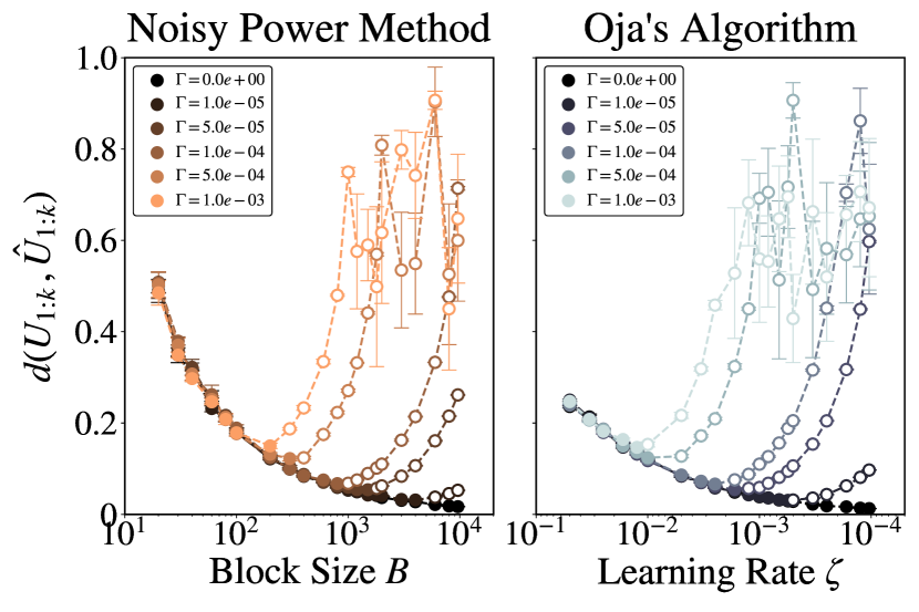
(a) Convergence of noisy power method and Oja’s algorithm. Variation with block size $B$ and learning rate $\zeta$ for $(\sigma,\delta,p,k,\Gamma)$=$(0.15,1.0,100,5,3.0e-5)$.

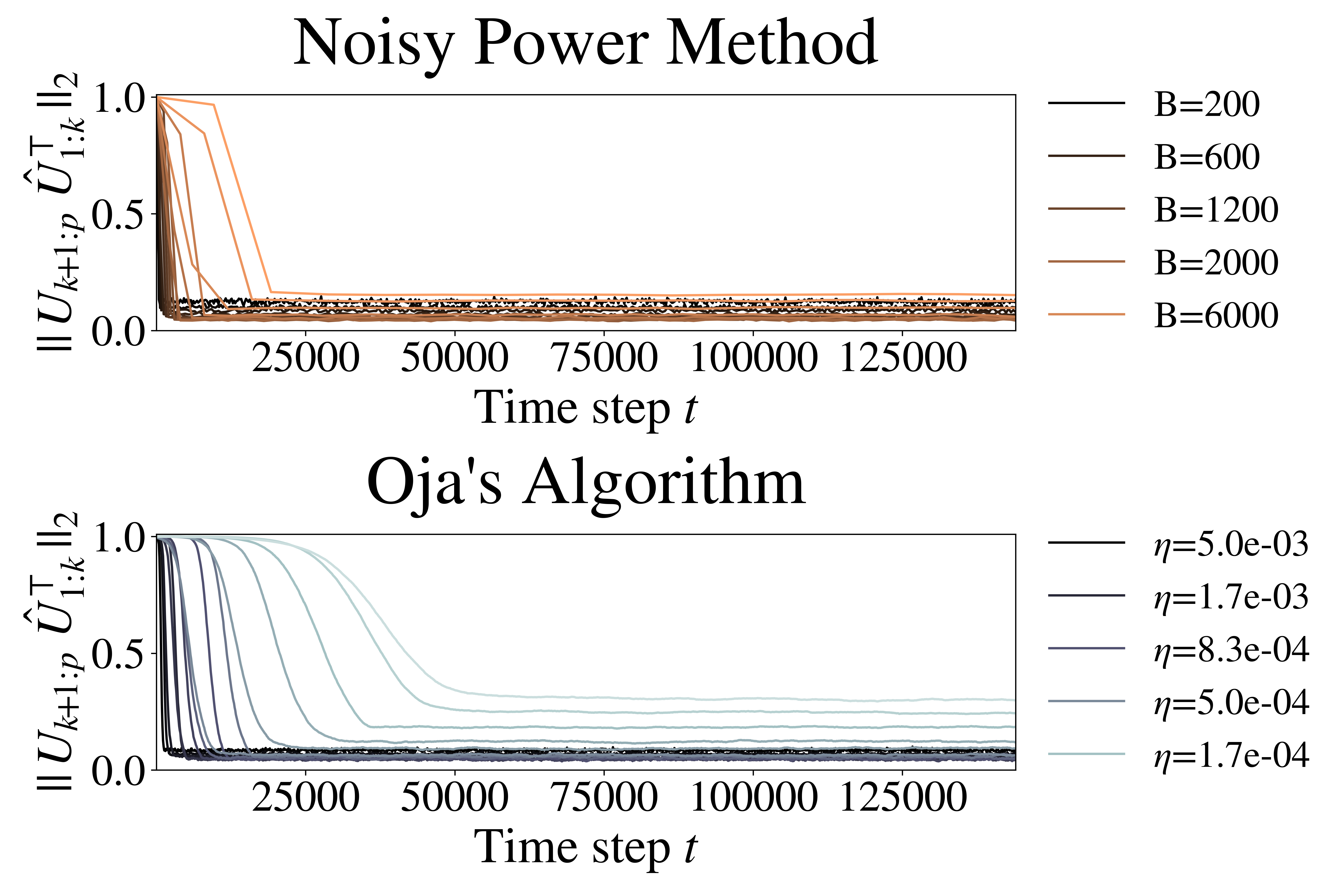
(b) Convergence of noisy power method and Oja’s algorithm, for bigger perturbations. $(\sigma,\delta,p,k)$=$(0.15,1.0,100,5)$.

Figure 3: Numerical results. We used the setting $(\sigma,\delta,p,k)\!=\!(0.15,1.0,100,5)$.

I.4 Details for each experiment

In this section, we expand on the computational setup used to generate Figure 1 and Figure 3.

For the Figure 1(a), we plot the distance between the estimated subspace and true space at the termination time $T$ for two algorithms with learning parameters at the Section I.2. We used four different $\Gamma$ : $[0.0,1.0e\!-\!5,3.0e\!-\!5,5.0e\!-\!5]$. We run the experiment 10 times, and plot error bar on each marker.

For Figure 3(a), we used same methodology with the Figure 1(a), but the larger perturbations $\Gamma$ : $[0.0,1.0e\!-\!5,5.0e\!-\!5,1.0e\!-\!4,5.0e\!-\!4,1.0e\!-\!3]$ were used. We ran 5 experiments each.

For the Figure 1(b), we find the empirically optimal value of the block size $B$ of the noisy power method and the learning rate $\zeta$ of Oja’s algorithm for various $\Gamma$. We first identify a lower and upper bound on the optimal value ($B$ and $\zeta$) from the simulations done for Figure 1(a) (For simulations for the Figure 1(a) we used learning parameters denoted in section I.2.) Once we identify upper and lower bounds for optimal value, we split the interval into 50 points and run each experiment with a fixed value of $B$ belonging to this interval for 30 runs. Finally, we calculate the average and standard deviation on those 30 runs. We denote 50 candidates for each $\Gamma$ with small dots. The optimal value incurring the least average convergence error is plotted as a big marker. Smaller markers for each $\Gamma$ denotes the parameter, which has lower $\texttt{avg}+\texttt{std}$ than the optimal value’s case.

In Figure 3(b), we visualize the convergence of two algorithms for various learning parameters, $B$, and $\zeta$. We reused the experiment result from Figure 1(a). The first observation from these experiments is that there is an optimal learning parameter that attains the minimum error (such behavior is in line with Theorem 2). Another key observation from these figures is that a smaller block size implies faster convergence; this is also in line with the dependence on the number of blocks ($L=T/{B}$) in Theorem 2.

Appendix J Experiment on the S&P500 Stock Dataset

J.1 Non-stationary in the Setting

To observe the distribution shift in this environment, we visualized the distance between covariance matrix with various window sizes and histogram for absolute values of daily return at the Figure 4. For the covariance distance, we first split the data stream into chunks with $w$ (window size) data each and calculated the covariance estimators. Then we plotted the operator 2-norm between the covariance matrix divided by $\sqrt{w}$. As the left figure displays, the distribution on this dataset shifts over time (the average distance is about 0.17). Furthermore, on the right, we visualized the counts for the absolute value of daily return with a logarithmic scale. We can observe a lot of zero elements and outliers. Note that both axes have a logarithmic scale.

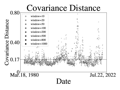
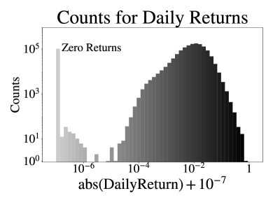
Figure 4: Non-stationary distribution characteristics of S&P500 stock market daily return. (Left): Distance of covariance matrix with window size variation and (Right): Histogram of the absolute value of daily returns.

J.2 Experimental Detail

We ran five experiments for each algorithm and $k=1,2,\ldots,5$, on the various regime of learning parameters ($B:1-1600$, $\eta:10^{-3.5}-10^{2.5}$). For the noisy power method, we just ignored the first $T\,\mathrm{mod}\,B$ data to approximate the final space properly.

References

- [1] K. Abed-Meraim, S. Attallah, A. Chkeif, and Y. Hua. Orthogonal oja algorithm. IEEE Signal Processing Letters, 7(5):116–119, 2000.
- [2] K. Abed-Meraim, A. Chkeif, and Y. Hua. Fast orthonormal past algorithm. IEEE Signal Processing Letters, 7(3):60–62, 2000.
- [3] Zeyuan Allen-Zhu and Yuanzhi Li. First efficient convergence for streaming k-pca: A global, gap-free, and near-optimal rate. In 2017 IEEE 58th Annual Symposium on Foundations of Computer Science (FOCS), pages 487–492, 2017.
- [4] Samreen Fatima and. THE APPLICATION OF PRINCIPAL COMPONENT ANALYSIS AND FACTOR ANALYSIS TO STOCK MARKETS RETURNS. International Journal of Advanced Research, 7(5):97–105, May 2019.
- [5] Raman Arora, Andrew Cotter, Karen Livescu, and Nathan Srebro. Stochastic optimization for pca and pls. In Communication, Control, and Computing (Allerton), 2012 50th Annual Allerton Conference on, pages 861–868. IEEE, 2012.
- [6] Laura Balzano, Robert Nowak, and Benjamin Recht. Online identification and tracking of subspaces from highly incomplete information. In 2010 48th Annual allerton conference on communication, control, and computing (Allerton), pages 704–711. IEEE, 2010.
- [7] Thomas Bendokat, Ralf Zimmermann, and P. A. Absil. A grassmann manifold handbook: Basic geometry and computational aspects, 2020.
- [8] Rajendra Bhatia. Matrix analysis, volume 169. Springer Science & Business Media, 2013.
- [9] Daniel Bienstock and Mauro Escobar. Stochastic defense against complex grid attacks. IEEE Transactions on Control of Network Systems, 7(2):842–854, 2020.
- [10] Daniel Bienstock and Apurv Shukla. Variance-aware optimal power flow: Addressing the tradeoff between cost, security, and variability. IEEE Transactions on Control of Network Systems, 6(3):1185–1196, 2019.
- [11] Vivek S Borkar. Stochastic approximation: a dynamical systems viewpoint, volume 48. Springer, 2009.
- [12] Florentina Bunea and Luo Xiao. On the sample covariance matrix estimator of reduced effective rank population matrices, with applications to fpca. Bernoulli, 21(2):1200–1230, 2015.
- [13] John Burkardt. The truncated normal distribution. Department of Scientific Computing Website, Florida State University, 1:35, 2014.
- [14] Tony Cai, Zongming Ma, and Yihong Wu. Optimal estimation and rank detection for sparse spiked covariance matrices. Probability Theory and Related Fields, 161(3):781–815, Apr 2015.
- [15] Emmanuel J Candès, Xiaodong Li, Yi Ma, and John Wright. Robust principal component analysis? Journal of the ACM (JACM), 58(3):1–37, 2011.
- [16] Minshuo Chen, Lin Yang, Mengdi Wang, and Tuo Zhao. Dimensionality reduction for stationary time series via stochastic nonconvex optimization. arXiv preprint arXiv:1803.02312, 2018.
- [17] Yeshwanth Cherapanamjeri, Prateek Jain, and Praneeth Netrapalli. Thresholding based outlier robust pca. In Conference on Learning Theory, pages 593–628. PMLR, 2017.
- [18] Yuejie Chi, Yonina C. Eldar, and Robert Calderbank. Petrels: Parallel subspace estimation and tracking by recursive least squares from partial observations. IEEE Transactions on Signal Processing, 61(23):5947–5959, 2013.
- [19] John H. Conway, Ronald H. Hardin, and Neil J. A. Sloane. Packing lines, planes, etc.: packings in Grassmannian spaces. Experimental Mathematics, 5(2):139 – 159, 1996.
- [20] Wei Dai, Youjian Liu, and B. Rider. Quantization bounds on grassmann manifolds of arbitrary dimensions and mimo communications with feedback. In GLOBECOM ’05. IEEE Global Telecommunications Conference, 2005., volume 3, pages 5 pp.–, 2005.
- [21] David Donoho, Matan Gavish, and Iain Johnstone. Optimal shrinkage of eigenvalues in the spiked covariance model. The Annals of Statistics, 46(4):1742 – 1778, 2018.
- [22] G.H. Dunteman. Principal Components Analysis. Number No. 69 in A Sage Publications. SAGE Publications, 1989.
- [23] Mauro Escobar, Daniel Bienstock, and Michael Chertkov. Learning from power system data stream. In 2019 IEEE Milan PowerTech, pages 1–6. IEEE, 2019.
- [24] Jiashi Feng, Huan Xu, and Shuicheng Yan. Online robust pca via stochastic optimization. In Advances in Neural Information Processing Systems, pages 404–412, 2013.
- [25] Mina Ghashami, Edo Liberty, Jeff M. Phillips, and David P. Woodruff. Frequent directions: Simple and deterministic matrix sketching. SIAM Journal on Computing, 45(5):1762–1792, 2016.
- [26] John Goes, Teng Zhang, Raman Arora, and Gilad Lerman. Robust stochastic principal component analysis. In Artificial Intelligence and Statistics, pages 266–274. PMLR, 2014.
- [27] Donald Goldfarb and Garud Iyengar. Robust portfolio selection problems. Mathematics of operations research, 28(1):1–38, 2003.
- [28] Gene H Golub and Charles F Van Loan. Matrix computations (4th ed), volume 3. JHU Press, 2012.
- [29] Moritz Hardt and Eric Price. The noisy power method: A meta algorithm with applications. In Advances in Neural Information Processing Systems, pages 2861–2869, 2014.
- [30] Jun He, Laura Balzano, and John C. S. Lui. Online Robust Subspace Tracking from Partial Information. arXiv e-prints, page arXiv:1109.3827, September 2011.
- [31] Amelia Henriksen and Rachel Ward. Adaoja: Adaptive learning rates for streaming pca, 2019.
- [32] De Huang, Jonathan Niles-Weed, Joel A Tropp, and Rachel Ward. Matrix concentration for products. arXiv preprint arXiv:2003.05437, 2020.
- [33] De Huang, Jonathan Niles-Weed, and Rachel Ward. Streaming k-pca: Efficient guarantees for oja’s algorithm, beyond rank-one updates. In Mikhail Belkin and Samory Kpotufe, editors, Conference on Learning Theory, COLT 2021, 15-19 August 2021, Boulder, Colorado, USA, volume 134 of Proceedings of Machine Learning Research, pages 2463–2498. PMLR, 2021.
- [34] Prateek Jain, Chi Jin, Sham M Kakade, Praneeth Netrapalli, and Aaron Sidford. Streaming pca: Matching matrix bernstein and near-optimal finite sample guarantees for oja’s algorithm. In Conference on Learning Theory, pages 1147–1164, 2016.
- [35] Iain M. Johnstone. On the distribution of the largest eigenvalue in principal components analysis. The Annals of Statistics, 29(2):295 – 327, 2001.
- [36] Iain M Johnstone and Debashis Paul. Pca in high dimensions: An orientation. Proceedings of the IEEE, 106(8):1277–1292, 2018.
- [37] Harold Kushner and G George Yin. Stochastic approximation and recursive algorithms and applications, volume 35. Springer Science & Business Media, 2003.
- [38] Chris Junchi Li, Mengdi Wang, Han Liu, and Tong Zhang. Near-optimal stochastic approximation for online principal component estimation. Mathematical Programming, 167(1):75–97, 2018.
- [39] Xin Liang. On the optimality of the oja’s algorithm for online PCA. CoRR, abs/2104.00512, 2021.
- [40] Edo Liberty. Simple and deterministic matrix sketching. In Proceedings of the 19th ACM SIGKDD International Conference on Knowledge Discovery and Data Mining, KDD ’13, page 581–588, New York, NY, USA, 2013. Association for Computing Machinery.
- [41] André L. G. Mandolesi. Grassmann angles between real or complex subspaces, 2021.
- [42] Poorya Mianjy and Raman Arora. Stochastic pca with and regularization. In ICML, 2018.
- [43] Ioannis Mitliagkas, Constantine Caramanis, and Prateek Jain. Memory limited, streaming pca. In Proceedings of the 26th International Conference on Neural Information Processing Systems - Volume 2, NIPS’13, page 2886–2894, Red Hook, NY, USA, 2013. Curran Associates Inc.
-
[44]
Paul Mooney.
Stock Market Data (NASDAQ, NYSE, S&P500).
https://www.kaggle.com/datasets/paultimothymooney/stock-market-data, Version 64. - [45] Jonas W Mueller, Vasilis Syrgkanis, and Matt Taddy. Low-rank bandit methods for high-dimensional dynamic pricing. Advances in Neural Information Processing Systems, 32, 2019.
- [46] Praneeth Narayanamurthy and Namrata Vaswani. Provable dynamic robust pca or robust subspace tracking. IEEE Transactions on Information Theory, 65(3):1547–1577, 2018.
- [47] Yuri Neretin. On jordan angles and the triangle inequality in grassmann manifolds. Geometriae Dedicata, 86:81–91, 06 2001.
- [48] Erkki Oja and Juha Karhunen. On stochastic approximation of the eigenvectors and eigenvalues of the expectation of a random matrix. Journal of mathematical analysis and applications, 106(1):69–84, 1985.
- [49] Daniel L Pimentel-Alarcón, Aritra Biswas, and Claudia R Solís-Lemus. Adversarial principal component analysis. In 2017 IEEE International Symposium on Information Theory (ISIT), pages 2363–2367. IEEE, 2017.
- [50] Olivier Roy and Martin Vetterli. The effective rank: A measure of effective dimensionality. In 2007 15th European signal processing conference, pages 606–610. IEEE, 2007.
- [51] Ohad Shamir. Convergence of stochastic gradient descent for pca. In International Conference on Machine Learning, pages 257–265, 2016.
- [52] Ohad Shamir. Fast stochastic algorithms for svd and pca: Convergence properties and convexity. In International Conference on Machine Learning, pages 248–256, 2016.
- [53] Wenjie Song, Jianke Zhu, Yang Li, and Chun Chen. Image alignment by online robust pca via stochastic gradient descent. IEEE Transactions on Circuits and Systems for video Technology, 26(7):1241–1250, 2015.
- [54] Wataru Souma. Characteristics of principal components in stock price correlation. Frontiers in Physics, 9, 2021.
- [55] Le Trung Thanh, Nguyen Viet Dung, Nguyen Linh Trung, and Karim Abed-Meraim. Robust subspace tracking with missing data and outliers: Novel algorithm with convergence guarantee. IEEE Transactions on Signal Processing, 69:2070–2085, 2021.
- [56] Joel A. Tropp. An introduction to matrix concentration inequalities. Foundations and Trends® in Machine Learning, 8(1-2):1–230, 2015.
- [57] Alexandre B Tsybakov. Introduction to nonparametric estimation. Springer Science & Business Media, 2008.
- [58] Vincent Q. Vu and Jing Lei. Minimax sparse principal subspace estimation in high dimensions. The Annals of Statistics, 41(6):2905 – 2947, 2013.
- [59] Sissi Xiaoxiao Wu, Hoi-To Wai, Anna Scaglione, and Neil A. Jacklin. The power-oja method for decentralized subspace estimation/tracking. In 2017 IEEE International Conference on Acoustics, Speech and Signal Processing (ICASSP), pages 3524–3528, 2017.
- [60] Bin Yang. Projection approximation subspace tracking. IEEE Transactions on Signal Processing, 43(1):95–107, 1995.
- [61] Libin Yang. An Application of Principal Component Analysis to Stock Portfolio Management. PhD thesis, Department of Economics and Finance, University of Canterbury, 2015.
- [62] Puyudi Yang, Cho-Jui Hsieh, and Jane-Ling Wang. History pca: A new algorithm for streaming pca. arXiv preprint arXiv:1802.05447, 2018.