Abstract

The main aim of the present paper is to establish the existence of a phase transition for the quantum Ising model with competing $XY$ interactions within the quantum Markov chain (QMC) scheme. In this scheme, we employ the $C^{*}$-algebraic approach to the phase transition problem. Note that these kinde of models do not have one-dimensional analogues, i.e. the considered model persists only on trees. It turns out that if the Ising part interactions vanish then the model with only competing $XY$-interactions on the Cayley tree of order two does not have a phase transition. By phase transition we mean the existence of two distinct QMC which are not quasi-equivalent and their supports do not overlap. Moreover, it is also shown that the QMC associated with the model have clustering property which implies that the von Neumann algebras corresponding to the states are factors.

1 Introduction

The study of magnetic systems with competing interactions in ordering is a fascinating problem of condensed matter physics. One of the most canonical examples of such systems are frustrated Ising models which demonstrate a plethora of critical properties[20, 28, 30]. The frustrations can be either geometrical or brought about the next-nearest neighbor NNN interactions. Competing interactions frustrations can result new phases, change the Ising universality class, or even destroy the order at all. Another interesting aspect of the criticality in the frustrated Ising models is an appearance of quantum critical points at spacial frustration points of model’s high degeneracy, and related quantum phase transitions [40]. The Ising models with frustrations can be thought as perturbation of the classical Ising model. If the perturbation terms do not commute with the Ising pieces, it outcomes quantum effects. In particular case, if the perturbation is the XY interaction, then the model become more interesting (see [12, 21, 30, 36] for a systematic study (physical approach) of the Ising model with quantum frustration on 2D lattices). However, a rigorous (mathematical) investigation of the quantum Ising model with competing $XY$ interactions does not exist yet in the literature. We notice that $XY$-interactions are truly quantum, ( i.e. contain pieces not commuting with each other). In the present paper, we propose to investigate the phase transition problem for the mentioned model on the Cayley tree or Bethe lattice [35] within quantum Markov chains (QMC) scheme. Here, the QMC scheme is based on the $C^{*}$-algebraic approach. We notice that the Ising model with Ising type competing interactions (with commuting interactions) has been recently studied in [31, 32, 33, 34] by means of QMC. As we mentioned, in the current paper, the commuting interactions are non-commutative, and this makes big difference between those papers.

On the other hand, our investigation will allow to construct quantum analogous of Markov fields (see [23, 27, 37, 42, 41]) which is one of the basic problems in quantum probability. We notice that quantum Markov fields naturally appear in quantum statistical mechanics and quantum fields theories [22, 24].

We point out, even in classical setting, for models over integer lattices, there do not exist analytical solutions (for example, critical temperature) on such lattices. Therefore, it was proposed [15] to consider spin models on regular trees for which one can exactly calculate various physical quantities. One of the simplest tree is a Cayley tree [35]. In [31, 32] we have established that Gibbs measures of the Ising model with competing (Ising) interactions on a Cayley trees, can be considered as QMC. Note that if the perturbation vanishes then the model reduces to the classical Ising one which was also examined in [13] by means of $C^{*}$-algebra approach.

In the present paper, we are going to study the Ising model with $XY$-competing interactions on a Cayley trees of order two. We point out that this model has non-commutative interactions, i.e. $XY$ ones, therefore, the investigation of this model is tricky. We notice that, in general, QMC do not have KMS property (see [4, 18]), therefore, general theory of KMS-states is not applicable for such kind of chains. One of the main questions of this paper is to know whether the considered model exhibits two different QMC associated with the mentioned model on the Cayley trees. Our main result is the following one.

Theorem 1.1.

For the Ising model with competing $XY$- interactions (18), (20), $J_{0}>0$, $J\in\mathbb{R}\setminus\{-J_{0},J_{0}\}$, $\beta>0$ on the Cayley tree of order two, the following statements hold:

• if $\Delta(\theta)\leq 0$, then there is a unique QMC;

• if $\Delta(\theta)>0$, then there occurs a phase transition,

where

$$\Delta(\theta)=\frac{\theta^{2J_{0}}-\theta^{J_{0}}(\theta^{J}+\theta^{-J})-3}{\theta^{2J_{0}}-\theta^{J_{0}}(\theta^{J}+\theta^{-J})+1},~{}~{}\theta=e^{2\beta}.$$

To establish result, we will prove Theorem 5.3, from which we conclude that there are three coexisting phases in the region $\Delta(\theta)>0$, and one of it, i.e. $\varphi_{\alpha}$, survives in the region $\Delta(\theta)<0$. This leads us that the state $\varphi_{\alpha}$ describes the disordered phase of the model, which shows a similar behavior with the classical Ising model [16, 38]. In comparison with the Ising model, we stress that in the present model, we have a similar kind of phases (translation invariant ones) when $\Delta(\theta)>0$. From Figure 2 (see below), one concludes that the phase transition occurs except for a ”triangular region”. This shows how the competing interactions effect to the existence of other phases. Notice that if $J=0$, then we obtain the classical Ising model for which the existence of a disordered phase coexisting with two ordered phases is well-known [15, 38].

On the other hand, we emphasize that both problems, i.e. a construction and phase transitions are non-trivial and, to a large extent, open. In fact, even if several definitions of quantum Markov fields on trees (and more generally on graphs) have been proposed, a really satisfactory, general theory is still missing and physically interesting examples of such fields in dimension $d\geq 2$ are very few.

In order to get the existence of the phase transition (see [31]), one needs to check several conditions, and one of them based on a notion of the quasi-equivalence of quantum Markov chains which essentially uses $C^{*}$-algebraic approach and techniques. This situation totally differs from the classical (resp. quantum) cases, where it is sufficient to prove the existence of at least two different solutions (resp. KMS states) of associated renormalized equations (see [38]). Therefore, even for classical models, to check the existence of the phase transition (in the sense of our paper) is not a trivial problem. Here we mention that the quasi-equivalence of product states (which correspond to the classical model without interactions) was a tricky job and investigated in [29, 39]. In this paper, we are considering more complicated states (which are QMC associated with the model) than product ones, and for these kind of states we are going to obtain their non-quasi equivalence. We will first show that these states have clustering property, and hence they are factor states. We point out that even this fact presents its own interests since these states associates with non-commutative Hamiltonians having non-trivial interactions.

Let us outline the organization of the paper. After preliminary information (see Section 2), in Section 3 we provide a general construction of backward quantum Markov chains on Cayley tree. Moreover, in this section we give the definition of the phase transition. Using the provided construction, in Section 4 we consider the Ising model with competing $XY$-interactions on the Cayley tree of order two. Section 5 is devoted to the existence of the three translation-invariant QMC $\varphi_{\alpha}$, $\varphi_{1}$ and $\varphi_{1}$ corresponding to the model. Section 6 is devoted to the proof of Theorem 1.1. In this section we will prove that states $\varphi_{1}$ and $\varphi_{2}$ do not have overlapping supports. Before, to establish their non-quasi equivalence, we first prove that these states have the clustering property. Section 7 we study a particular case $J_{0}=0$, which means that we only have $XY$ interactions. In the considered setting, it turns out that the phase transition does not occur.

2 Preliminaries

Let $\Gamma^{k}_{+}=(L,E)$ be a semi-infinite Cayley tree of order $k\geq 1$ with the root $x^{0}$ (i.e. each vertex of $\Gamma^{k}_{+}$ has exactly $k+1$ edges, except for the root $x^{0}$, which has $k$ edges). Here $L$ is the set of vertices and $E$ is the set of edges. The vertices $x$ and $y$ are called nearest neighbors and they are denoted by $l=<x,y>$ if there exists an edge connecting them. A collection of the pairs $<x,x_{1}>,\dots,<x_{d-1},y>$ is called a path from the point $x$ to the point $y$. The distance $d(x,y),x,y\in V$, on the Cayley tree, is the length of the shortest path from $x$ to $y$.

Recall a coordinate structure in $\Gamma^{k}_{+}$: every vertex $x$ (except for $x^{0}$) of $\Gamma^{k}_{+}$ has coordinates $(i_{1},\dots,i_{n})$, here $i_{m}\in\{1,\dots,k\}$, $1\leq m\leq n$ and for the vertex $x^{0}$ we put $(0)$. Namely, the symbol $(0)$ constitutes level 0, and the sites $(i_{1},\dots,i_{n})$ form level $n$ (i.e. $d(x^{0},x)=n$) of the lattice (see Fig. 1).

Figure 1: The first levels of $\Gamma_{+}^{2}$

Let us set

$$W_{n}=\{x\in L\,:\,d(x,x_{0})=n\},\qquad\Lambda_{n}=\bigcup_{k=0}^{n}W_{k},\qquad\Lambda_{[n,m]}=\bigcup_{k=n}^{m}W_{k},{\mathcal{C}}(n<m)$$

$$E_{n}=\big{\{}<x,y>\in E\,:\,x,y\in\Lambda_{n}\big{\}},\qquad\Lambda_{n}^{c}=\bigcup_{k=n}^{\infty}W_{k}$$

For $x\in\Gamma^{k}_{+}$, $x=(i_{1},\dots,i_{n})$ denote

$$S(x)=\{(x,i):{\mathcal{C}}1\leq i\leq k\}.$$

Here $(x,i)$ means that $(i_{1},\dots,i_{n},i)$. This set is called a set of direct successors of $x$.

Two vertices $x,y\in V$ is called one level next-nearest-neighbor vertices if there is a vertex $z\in V$ such that $x,y\in S(z)$, and they are denoted by $>x,y<$. In this case the vertices $x,z,y$ was called ternary and denoted by $<x,z,y>$.

Let us define on $\Gamma^{k}_{+}$ a binary operation $\circ:\Gamma^{k}_{+}\times\Gamma^{k}_{+}\to\Gamma^{k}_{+}$ as follows: for any two elements $x=(i_{1},\dots,i_{n})$ and $y=(j_{1},\dots,j_{m})$ put

$$x\circ y=(i_{1},\dots,i_{n})\circ(j_{1},\dots,j_{m})=(i_{1},\dots,i_{n},j_{1},\dots,j_{m})$$ (1)

and

$$x\circ x^{0}=x^{0}\circ x=(i_{1},\dots,i_{n})\circ(0)=(i_{1},\dots,i_{n}).$$ (2)

By means of the defined operation $\Gamma^{k}_{+}$ becomes a noncommutative semigroup with a unit. Using this semigroup structure one defines translations $\tau_{g}:\Gamma^{k}_{+}\to\Gamma^{k}_{+}$, $g\in\Gamma^{k}_{+}$ by

$$\tau_{g}(x)=g\circ x.$$ (3)

It is clear that $\tau_{(0)}=id$.

The algebra of observables ${\mathcal{B}}_{x}$ for any single site $x\in L$ will be taken as the algebra $M_{d}$ of the complex $d\times d$ matrices. The algebra of observables localized in the finite volume $\Lambda\subset L$ is then given by ${\mathcal{B}}_{\Lambda}=\bigotimes\limits_{x\in\Lambda}{\mathcal{B}}_{x}$. As usual if $\Lambda^{1}\subset\Lambda^{2}\subset L$, then ${\mathcal{B}}_{\Lambda^{1}}$ is identified as a subalgebra of ${\mathcal{B}}_{\Lambda^{2}}$ by tensoring with unit matrices on the sites $x\in\Lambda^{2}\setminus\Lambda^{1}$. Note that, in the sequel, by ${\mathcal{B}}_{\Lambda,+}$ we denote the positive part of ${\mathcal{B}}_{\Lambda}$. The full algebra ${\mathcal{B}}_{L}$ of the tree is obtained in the usual manner by an inductive limit

$${\mathcal{B}}_{L}=\overline{\bigcup\limits_{\Lambda_{n}}{\mathcal{B}}_{\Lambda_{n}}}.$$

In what follows, by ${\mathcal{S}}({\mathcal{B}}_{\Lambda})$ we will denote the set of all states defined on the algebra ${\mathcal{B}}_{\Lambda}$.

Consider a triplet ${\mathcal{C}}\subset{\mathcal{B}}\subset{\mathcal{A}}$ of unital $C^{*}$-algebras. Recall [2] that a quasi-conditional expectation with respect to the given triplet is a completely positive (CP) linear map $\mathcal{E}\,:\,{\mathcal{A}}\to{\mathcal{B}}$ such that $\mathcal{E}(ca)=c\mathcal{E}(a)$, for all $a\in{\mathcal{A}},\,c\in{\mathcal{C}}$.

Definition 2.1 ([10]).

A state $\varphi$ on ${\mathcal{B}}_{L}$ is called a backward quantum Markov chain (QMC), associated to $\{\Lambda_{n}\}$, if for each $\Lambda_{n}$, there exist a quasi-conditional expectation $\mathcal{E}_{\Lambda_{n}}$ with respect to the triplet

$${\mathcal{B}}_{{\Lambda}_{n-1}}\subseteq{\mathcal{B}}_{\Lambda_{n}}\subseteq{\mathcal{B}}_{\Lambda_{n+1}}$$ (4)

and an initial state $\rho\in S(B_{\Lambda_{0}})$ such that:

$$\varphi=\lim_{n\to\infty}\rho_{0}\circ\mathcal{E}_{\Lambda_{0}}\circ\mathcal{E}_{\Lambda_{1}}\circ\cdots\circ\mathcal{E}_{\Lambda_{n}}$$ (5)

in the weak-* topology.

Remark 2.2.

We notice that in [6] a more general definition of backward QMC is given on arbitrary quasi-local algebras.

3 Construction of Quantum Markov Chains

In this section we are going to provide a construction of a backward quantum Markov chain which contains competing interactions.

Let us rewrite the elements of $W_{n}$ in the following lexicographic order (w.r.t. the coordinate system), i.e.

$$\overrightarrow{W_{n}}:=\left(x^{(1)}_{W_{n}},x^{(2)}_{W_{n}},\cdots,x^{(|W_{n}|)}_{W_{n}}\right).$$

Note that $|W_{n}|=k^{n}$. In this lexicographic order, vertices $x^{(1)}_{W_{n}},x^{(2)}_{W_{n}},\cdots,x^{(|W_{n}|)}_{W_{n}}$ of $W_{n}$ are given as follows

$$x^{(1)}_{W_{n}}=(1,1,\cdots,1,1),\quad x^{(2)}_{W_{n}}=(1,1,\cdots,1,2),{\mathcal{C}}{\mathcal{C}}\cdots\quad x^{(k)}_{W_{n}}=(1,1,\cdots,1,k,),$$ (6)

$$x^{(k+1)}_{W_{n}}=(1,1,\cdots,2,1),\quad x^{(2)}_{W_{n}}=(1,1,\cdots,2,2),{\mathcal{C}}{\mathcal{C}}\cdots\quad x^{(2k)}_{W_{n}}=(1,1,\cdots,2,k),$$

$$\vdots$$

$$x^{(|W_{n}|-k+1)}_{W_{n}}=(k,k,,\cdots,k,1),{\mathcal{C}}x^{(|W_{n}|-k+2)}_{W_{n}}=(k,k,\cdots,k,2),{\mathcal{C}}{\mathcal{C}}\cdots x^{|W_{n}|}_{W_{n}}=(k,k,\cdots,k,k).$$

Analogously, for a given vertex $x,$ we shall use the following notation for the set of direct successors of $x$:

$$\overrightarrow{S(x)}:=\left((x,1),(x,2),\cdots(x,k)\right),\quad\overleftarrow{S(x)}:=\left((x,k),(x,k-1),\cdots(x,1)\right).$$

In what follows, by ${}^{\circ}\prod$ we denote the lexicographic order, i.e.

$${}^{\circ}\prod_{k=1}^{n}a_{k}=a_{1}a_{2}\cdots a_{n},$$

where elements $\{a_{k}\}\subset{\mathcal{B}}_{L}$ are multiplied in the indicated order. This means that we are not allowed to change this order.

Note that each vertex $x\in L$ has interacting vertices $\{x,(x,1),\dots,(x,k)\}$. Assume that, to each edges $<x,(x,i)>$ ($i=1,\dots,k$) an operators $K_{<x,(x,i)>}\in\mathcal{B}_{x}\otimes\mathcal{B}_{(x,i)}$ is assigned, respectively. Moreover, for each competing vertices $>(x,i),(x,i+1)<$ and $<x,(x,i),(x,i+1)>$ ($i=1,\dots,k$) the following operators are assigned:

$$L_{>(x,i),(x,i+1)<}\in\mathcal{B}_{(x,i)}\otimes\mathcal{B}_{(x,i+1)},{\mathcal{C}}{\mathcal{C}}M_{(x,(x,i),(x,i+1))}\in\mathcal{B}_{x}\otimes\mathcal{B}_{(x,i)}\otimes\mathcal{B}_{(x,i+1)}.$$

We would like to define a state on $\mathcal{B}_{\Lambda_{n}}$ with boundary conditions $\omega_{0}\in\mathcal{B}_{0,+}$ and $\{h^{x}\in\mathcal{B}_{x,+}:{\mathcal{C}}x\in L\}$.

For each $n\in\mathbf{N}$ denote

$$A_{x,(x,1),\dots,(x,k)}=\big{(}^{\circ}\prod_{i=1}^{k}K_{x,(x,i)}\big{)}\big{(}^{\circ}\prod_{i=1}^{k}L_{>(x,i),(x,i+1)<}\big{)}\big{(}^{\circ}\prod_{i=1}^{k}M_{(x,(x,i),(x,i+1))}\big{)},$$ (7)

$$K_{[m,m+1]}:=\prod_{x\in\overrightarrow{W}_{m}}A_{x,(x,1),\dots,(x,k)},{\mathcal{C}}{\mathcal{C}}1\leq m\leq n,$$ (8)

$$\mathbf{h}_{n}^{1/2}:=\prod_{x\in W_{n}}(h^{x})^{1/2},{\mathcal{C}}{\mathcal{C}}{\mathcal{C}}\mathbf{h}_{n}=\mathbf{h}_{n}^{1/2}(\mathbf{h}_{n}^{1/2})^{*}$$ (9)

$${\mathbf{K}}_{n}:=\omega_{0}^{1/2}(^{\circ}\prod_{m=0}^{n-1}K_{[m,m+1]})\mathbf{h}_{n}^{1/2}$$ (10)

$$\mathcal{W}_{n]}:={\mathbf{K}}_{n}^{*}{\mathbf{K}}_{n}$$ (11)

One can see that ${\mathcal{W}}_{n]}$ is positive.

In what follows, by ${\rm Tr}_{\Lambda}:{\mathcal{B}}_{L}\to{\mathcal{B}}_{\Lambda}$ we mean normalized partial trace (i.e. ${\rm Tr}_{\Lambda}({\bf 1}\!\!{\rm I}_{L})={\bf 1}\!\!{\rm I}_{\Lambda}$, here ${\bf 1}\!\!{\rm I}_{\Lambda}=\bigotimes\limits_{y\in\Lambda}{\bf 1}\!\!{\rm I}$), for any $\Lambda\subseteq_{\text{fin}}L$. For the sake of shortness we put ${\rm Tr}_{n]}:={\rm Tr}_{\Lambda_{n}}$.

Let us define a positive functional $\varphi^{(n)}_{w_{0},\mathbf{h}}$ on ${\mathcal{B}}_{\Lambda_{n}}$ by

$$\varphi^{(n)}_{w_{0},\mathbf{h}}(a)={\rm Tr}(\mathcal{W}_{n+1]}(a\otimes{\bf 1}\!\!{\rm I}_{W_{n+1}})),$$ (12)

for every $a\in{\mathcal{B}}_{\Lambda_{n}}$. Note that here, ${\rm Tr}$ is a normalized trace on ${\mathcal{B}}_{L}$ (i.e. ${\rm Tr}({\bf 1}\!\!{\rm I}_{L})=1$).

To get an infinite-volume state $\varphi$ on ${\mathcal{B}}_{L}$ such that $\varphi\lceil_{{\mathcal{B}}_{\Lambda_{n}}}=\varphi^{(n)}_{w_{0},\mathbf{h}}$, we need to impose some constrains to the boundary conditions $\big{\{}w_{0},\mathbf{h}\big{\}}$ so that the functionals $\{\varphi^{(n)}_{w_{0},\mathbf{h}}\}$ satisfy the compatibility condition, i.e.

$$\varphi^{(n+1)}_{w_{0},\mathbf{h}}\lceil_{{\mathcal{B}}_{\Lambda_{n}}}=\varphi^{(n)}_{w_{0},\mathbf{h}}.$$ (13)

Theorem 3.1.

Assume that for every $x\in L$ and triple $\{x,(x,i),(x,i+1)\}$ $(i=1,\dots,k-1$) the operators $K_{<x,(x,i)>}$, $L_{>(x,i),(x,i+1)<}$, $M_{(x,(x,i),(x,i+1))}$ are given as above. Let the boundary conditions $w_{0}\in{\mathcal{B}}_{(0),+}$ and ${\mathbf{h}}=\{h_{x}\in{\mathcal{B}}_{x,+}\}_{x\in L}$ satisfy the following conditions:

$$\mathrm{Tr}(\omega_{0}h_{0})=1,$$ (14)

$$\mathrm{Tr}_{x]}\big{(}{A_{x,(x,1),\dots,(x,k)}}^{\circ}\prod_{i=1}^{k}h^{(x,i)}A_{x,(x,1),\dots,(x,k)}^{*}\big{)}=h^{x},{\mathcal{C}}{\mathcal{C}}\textrm{for every}{\mathcal{C}}{\mathcal{C}}x\in L,$$ (15)

where as before $A_{x,(x,1),\dots,(x,k)}$ is given by (7). Then the functionals $\{\varphi^{(n)}_{w_{0},\mathbf{h}}\}$ satisfy the compatibility condition (13). Moreover, there is a unique backward quantum d-Markov chain $\varphi_{w_{0},{\mathbf{h}}}$ on ${\mathcal{B}}_{L}$ such that $\varphi_{w_{0},{\mathbf{h}}}=w-\lim\limits_{n\to\infty}\varphi^{(n)}_{w_{0},\mathbf{h}}$.

Proof.

Let us check that the states $\varphi^{(n,b)}_{w_{0},{\mathbf{h}}}$ satisfy the compatibility condition. For $a\in B_{\Lambda_{n}}$, we have:

$\varphi^{(n+1)}_{w_{0},{\mathbf{h}}}(a\otimes{\bf 1}\!\!{\rm I}_{\mathcal{W}_{n+1}})={\rm Tr}(\mathcal{W}_{n+2]}(a\otimes{\bf 1}\!\!{\rm I}_{\Lambda_{[n+1,n+2]}}))$
$={\rm Tr}(K_{[n,n+1]}^{*}K_{[n-1,n]}^{*}\cdots K_{[0,1]}^{*}w_{0}K_{[0,1]}K_{[1,2]}\cdots K_{[n+1,n+2]}\mathbf{h}_{n+2}^{1/2}(a\otimes{\bf 1}\!\!{\rm I}_{\Lambda_{[n+1,n+2]}})\mathbf{h}_{n+2}^{1/2}K_{[n+1,n+2]}^{*})$
$={\rm Tr}(K_{[n,n+1]}^{*}K_{[n-1,n]}^{*}\cdots K_{[0,1]}^{*}w_{0}K_{[0,1]}K_{[1,2]}\cdots K_{[n,n+1]}(a\otimes{\bf 1}\!\!{\rm I}_{\Lambda_{[n+1,n+2]}})K_{[n+1,n+2]}\mathbf{h}_{n+2}K_{[n+1,n+2]}^{*})$
$={\rm Tr}(K_{[n,n+1]}^{*}K_{[n-1,n]}^{*}\cdots K_{[0,1]}^{*}w_{0}K_{[0,1]}K_{[1,2]}\cdots K_{[n,n+1]}(a\otimes{\bf 1}\!\!{\rm I}_{\Lambda_{[n+1,n+2]}})\mathrm{Tr}_{n+1]}(K_{[n+1,n+2]}\mathbf{h}_{n+2}K_{[n+1,n+2]}^{*}))$
$={\rm Tr}(K_{[n,n+1]}^{*}K_{[n-1,n]}^{*}\cdots K_{[0,1]}^{*}w_{0}K_{[0,1]}K_{[1,2]}\cdots K_{[n,n+1]}(a\otimes{\bf 1}\!\!{\rm I}_{\Lambda_{[n+1,n+2]}})\mathbf{h}_{n+1})$
$={\rm Tr}(\mathbf{h}_{n+1}^{1/2}K_{[n,n+1]}^{*}K_{[n-1,n]}^{*}\cdots K_{[0,1]}^{*}w_{0}K_{[0,1]}K_{[1,2]}\cdots K_{[n,n+1]}\mathbf{h}_{n+1}^{1/2}(a\otimes{\bf 1}\!\!{\rm I}_{\Lambda_{[n+1,n+2]}}))$
$={\rm Tr}(\mathcal{W}_{n+1]}(a\otimes{\bf 1}\!\!{\rm I}_{\Lambda_{[n+1,n+2]}}))$
$=\varphi^{(n)}_{w_{0},{\mathbf{h}}}(a)$

To show that $\varphi^{(n)}_{w_{0},{\mathbf{h}}}$ is a backward QMC, we define quasi-conditional expectations $\mathcal{E}_{n}$ as follows:

$$\hat{\mathcal{E}}_{n}(x_{n+1]})={\rm Tr}_{n]}(K_{[n,n+1]}\mathbf{h}_{n+1}^{1/2}x_{n+1]}\mathbf{h}_{n+1}^{1/2}K_{[n,n+1]}^{*}),{\mathcal{C}}{\mathcal{C}}x_{n+1]}\in{\mathcal{B}}_{\Lambda_{n+1}}$$ (16)

$$\mathcal{E}_{k}(x_{k+1]})={\rm Tr}_{k]}(K_{[k,k+1]}x_{k+1]}K_{[k,k+1]}^{*}),{\mathcal{C}}{\mathcal{C}}x_{k+1]}\in{\mathcal{B}}_{\Lambda_{k+1}},{\mathcal{C}}{\mathcal{C}}k=1,2,\dots,n-1,$$ (17)

Then for any monomial $a_{\Lambda_{1}}\otimes a_{W_{2}}\otimes\cdots\otimes a_{W_{n}}\otimes{\bf 1}\!\!{\rm I}_{W_{n+1}}$, where $a_{\Lambda_{1}}\in{\mathcal{B}}_{\Lambda_{1}},a_{W_{k}}\in{\mathcal{B}}_{W_{k}}$, ($k=2,\dots,n$), we have:
$\varphi^{(n)}_{w_{0},\mathbf{h}}(a_{\Lambda_{1}}\otimes\cdots\otimes a_{W_{n}})={\rm Tr}(\mathcal{W}_{n+1]}(a_{\Lambda_{1}}\otimes\cdots\otimes a_{W_{n}}\otimes{\bf 1}\!\!{\rm I}_{W_{n+1}}))$
$={\rm Tr}(w_{0}K_{[0,1]}\cdots K_{[n,n+1]}\mathbf{h}_{n+1}^{1/2}(a_{\Lambda_{1}}\otimes\cdots\otimes a_{W_{n}}\otimes{\bf 1}\!\!{\rm I}_{W_{n+1}})\mathbf{h}_{n+1}^{1/2}K_{[n,n+1]}^{*}\cdots K_{[0,1]}^{*})\\$$={\rm Tr}(w_{0}K_{[0,1]}\cdots K_{[n-1,n]}{\rm Tr}_{n]}(K_{[n,n+1]}\mathbf{h}_{n+1}^{1/2}(a_{\Lambda_{1}}\otimes\cdots\otimes a_{W_{n}}\otimes{\bf 1}\!\!{\rm I}_{W_{n+1}})\mathbf{h}_{n+1}^{1/2}K_{[n,n+1]}^{*})K_{[n-1,n]}^{*}\cdots K_{[0,1]}^{*})\\$$={\rm Tr}(w_{0}K_{[0,1]}\cdots K_{[n-2,n-1]}{\rm Tr}_{n-1]}(K_{[n-1,n]}\hat{\mathcal{E}}_{n}(a_{\Lambda_{1}}\otimes\cdots\otimes a_{W_{n}})K_{[n-1,n]}^{*})\cdots K_{[0,1]}^{*})\\$$={\rm Tr}(w_{0}K_{[0,1]}\cdots K_{[n-2,n-1]}\mathcal{E}_{n-1}\hat{\mathcal{E}}_{n}(a_{\Lambda_{1}}\otimes\cdots\otimes a_{W_{n}})K_{[n-2,n-1]}^{*}\cdots K_{[0,1]}^{*})\\$$={\rm Tr}(w_{0}\mathcal{E}_{0}\circ\mathcal{E}_{1}\cdots\mathcal{E}_{n-1}\circ\hat{\mathcal{E}}_{n}(a_{\Lambda_{1}}\otimes\cdots\otimes a_{W_{n}}))$. This means that the limit state $\varphi_{w_{0},\mathbf{h}}$ is a backward QMC. This completes the proof. ∎

We notice that a phase transition phenomena is crucial in higher dimensional quantum models [17],[40, 19]. In [13], quantum phase transition for the two-dimensional Ising model using $C^{*}$-algebra approach. In [25] the VBS-model was considered on the Cayley tree. It was established the existence of the phase transition for the model in term of finitely correlated states which describe ground states of the model. Note that more general structure of finitely correlated states was studied in [26].

Our goal in this paper is to establish the existence of phase transition for the given family of operators. Heuristically, the phase transition means the existence of two distinct B backward QMC. Let us provide a more exact definition (see [31]).

Definition 3.2.

We say that there exists a phase transition for a family of operators $\{K_{<x,(x,i)>}\}$, $\{L_{>(x,i),(x,i+1)<}\}$, $\{M_{(x,(x,i),(x,i+1))}\}$ if the following conditions are satisfied:

1. existence: The equations (14), (15) have at least two $(u_{0},\{h^{x}\}_{x\in L})$ and $(v_{0},\{s^{x}\}_{x\in L})$ solutions;

2. not overlapping supports: there is a projector $P\in B_{L}$ such that $\varphi_{u_{0},\mathbf{h}}(P)<\varepsilon$ and $\varphi_{v_{0},\mathbf{s}}(P)>1-\varepsilon$, for some $\varepsilon>0$.

3. not quasi-equivalence: the corresponding quantum Markov chains $\varphi_{u_{0},\mathbf{h}}$ and $\varphi_{v_{0},\mathbf{s}}$ are not quasi equivalent .

Otherwise, we say there is no phase transition.

4 QMC associated with Ising-XY model with competing interactions

In this section, we define the model and formulate the main results of the paper. In what follows we consider a semi-infinite Cayley tree $\Gamma^{2}_{+}=(L,E)$ of order two. Our starting $C^{*}$-algebra is the same ${\mathcal{B}}_{L}$ but with ${\mathcal{B}}_{x}=M_{2}({\mathbb{C}})$ for all $x\in L$. By $\sigma_{x}^{u}$, $\sigma_{y}^{u}$, $\sigma_{z}^{u}$ we denote the Pauli spin operators for a site $u\in L$, i.e.

$${\bf 1}\!\!{\rm I}^{(u)}=\begin{pmatrix}0&1\\ 1&0\end{pmatrix},\sigma_{x}^{u}=\begin{pmatrix}0&1\\ 1&0\end{pmatrix},\sigma_{y}^{u}=\begin{pmatrix}0&-i\\ i&0\end{pmatrix},\sigma_{z}^{u}=\begin{pmatrix}1&0\\ 0&-1\end{pmatrix}.$$

For every vertices $(u,(u,1),(u,2))$ we put

$$K_{<u,(u,i)>}=\exp\{J_{0}\beta H_{<u,(u,i)>}\},{\mathcal{C}}{\mathcal{C}}i=1,2,{\mathcal{C}}{\mathcal{C}}J_{0}>0,{\mathcal{C}}\beta>0,$$ (18)

$$L_{>(u,1),(u,2)<}=\exp\{J\beta H_{>(u,1),(u,2)<}\},{\mathcal{C}}{\mathcal{C}}J\in{\mathbb{R}},$$ (19)

where

$$H_{<u,(u,1)>}=\frac{1}{2}\big{(}{\bf 1}\!\!{\rm I}^{(u)}\otimes{\bf 1}\!\!{\rm I}^{(u,1)}+\sigma_{z}^{(u)}\otimes\sigma_{z}^{(u,1)}\big{)},$$ (20)

$$H_{>(u,1),(u,2)<}=\frac{1}{2}\big{(}\sigma_{x}^{(u,1)}\otimes\sigma_{x}^{(u,2)}+\sigma_{y}^{(u,1)}\otimes\sigma_{y}^{(u,2)}\big{)}.$$ (21)

Furthermore, for the sake of simplicity, we assume that $M_{(u,(u,i),(u,i+1))}={\bf 1}\!\!{\rm I}$ ($i=1,2,\dots,k$) for all $u\in L$.

The defined model is called the Ising model with competing $XY$- interactions per vertices $(u,(u,1),(u,2))$.

For each $m\in\mathbb{N}$, from (20), (21) it follows that

$$H_{<u,v>}^{m}=H_{<u,v>}=\frac{1}{2}\big{(}{\bf 1}\!\!{\rm I}^{(u)}\otimes{\bf 1}\!\!{\rm I}^{(v)}+\sigma^{(u)}_{z}\otimes\sigma^{(v)}_{z}\big{)},$$ (22)

$$H_{>(u,1),(u,2)<}^{2m}=H_{>(u,1),(u,2)<}^{2}=\frac{1}{2}({\bf 1}\!\!{\rm I}^{(u,1)}\otimes{\bf 1}\!\!{\rm I}^{(u,2)}-\sigma_{z}^{(u,1)}\otimes\sigma_{z}^{(u,2)})$$ (23)

$$H_{>(u,1),(u,2)<}^{2m-1}=H_{>(u,1),(u,2)<}\big{.}$$ (24)

Therefore, one finds

$$K_{<u,(u,i)>}=K_{0}{\bf 1}\!\!{\rm I}^{(u)}\otimes{\bf 1}\!\!{\rm I}^{(u,i)}+K_{3}\sigma_{z}^{(u)}\otimes\sigma_{z}^{(u,i)}$$

$$L_{>(u,1),(u,2)<}={\bf 1}\!\!{\rm I}^{(u,1)}\otimes{\bf 1}\!\!{\rm I}^{(u,2)}+\sinh(J\beta)H_{>(u,1),(u,2)<}+(\cosh(J\beta)-1)H^{2}_{>(u,1),(u,2)<}$$

where

$$K_{0}=\frac{\exp{J_{0}\beta}+1}{2},{\mathcal{C}}{\mathcal{C}}{\mathcal{C}}K_{3}=\frac{J_{0}\exp{\beta}-1}{2},$$

Hence, from (7) for each $x\in L$ we obtain

$$A_{(u,(u,1),(u,2))} =\gamma_{1}{\bf 1}\!\!{\rm I}^{(u)}\otimes{\bf 1}\!\!{\rm I}^{(u,1)}\otimes{\bf 1}\!\!{\rm I}^{(u,2)}+\gamma_{2}{\bf 1}\!\!{\rm I}^{u}\otimes\sigma_{x}^{(u,1)}\otimes\sigma_{x}^{(u,2)}$$ (25)

$$+\gamma_{2}{\bf 1}\!\!{\rm I}^{(u)}\otimes\sigma_{y}^{(u,1)}\otimes\sigma_{y}^{(u,2)}+\gamma_{3}{\bf 1}\!\!{\rm I}^{(u)}\otimes\sigma_{z}^{(u,1)}\otimes\sigma_{z}^{(u,2)}$$

$$+\delta_{1}\sigma_{z}^{(u)}\otimes{\bf 1}\!\!{\rm I}^{(u,1)}\otimes\sigma_{z}^{(u,2)}+\delta_{1}\sigma_{z}^{(u)}\otimes\sigma_{z}^{(u,1)}\otimes{\bf 1}\!\!{\rm I}^{(u,2)}$$

where

$$\left\{\begin{matrix}\gamma_{1}=\frac{1}{4}[\exp(2J_{0}\beta)+1+2\exp(J_{0}\beta)\cosh(J\beta)],&\gamma_{2}=\frac{1}{2}\exp(J_{0}\beta)\sinh(J\beta).\vskip 12.0pt plus 4.0pt minus 4.0pt\\ \gamma_{3}=\frac{1}{4}[\exp(2J_{0}\beta)+1-2\exp(J_{0}\beta)\cosh(J\beta)],&\delta_{1}=\frac{1}{4}(\exp(2J_{0}\beta)-1).\end{matrix}\right.$$

Recall that a function $\{h^{u}\}$ is called translation-invariant if one has $h^{u}=h^{\tau_{g}(u)}$, for all $u,g\in\Gamma^{2}_{+}$. Clearly, this is equivalent to $h^{u}=h^{v}$ for all $u,v\in L$.

In what follows, we restrict ourselves to the description of translation-invariant solutions of (14),(15). Consequently, we assume that: $h^{u}=h$ for all $u\in L$, here

$$h=\left(\begin{array}[]{cc}h_{11}&h_{12}\\ h_{21}&h_{22}\\ \end{array}\right).$$

Then, equation (15) reduces to

$$h = \mathrm{Tr}_{u]}A_{(u,(u,1),(u,2))}[{\bf 1}\!\!{\rm I}^{(u)}\otimes h\otimes h]A_{(u,(u,1),(u,2))}^{*}$$ (26)

$$= [C_{1}{\rm Tr}(h)^{2}+C_{2}{\rm Tr}(\sigma_{z}h)^{2}]{\bf 1}\!\!{\rm I}^{(u)}+C_{3}Tr(h)\mathrm{Tr}(\sigma_{z}h)\sigma_{z}^{(u)}.$$

where

$$\left\{\begin{array}[]{ll}C_{1}=\frac{1}{4}(\exp(4J_{0}\beta)+1)+\frac{1}{2}\exp(2J_{0}\beta)\cosh(2J\beta);\vskip 12.0pt plus 4.0pt minus 4.0pt\\ C_{2}=\frac{1}{4}(\exp(4J_{0}\beta)+1)-\frac{1}{2}\exp(2J_{0}\beta)\cosh(2J\beta);\vskip 12.0pt plus 4.0pt minus 4.0pt\\ C_{3}=\frac{1}{2}(\exp(4J_{0}\beta)-1).\end{array}\right.$$

Now taking into account

$$\mathrm{Tr}(h)=\frac{h_{11}+h_{22}}{2},{\mathcal{C}}{\mathcal{C}}\mathrm{Tr}(\sigma_{z}h)=\frac{h_{11}-h_{22}}{2}$$

the equation (26) reduces to the following one

$$\left\{\begin{array}[]{lll}\mathrm{Tr}(h)=C_{1}\mathrm{Tr}(h)^{2}+C_{2}\mathrm{Tr}(\sigma h)^{2},\\ \mathrm{Tr}(\sigma h)=C_{3}\mathrm{Tr}(h)\mathrm{Tr}(\sigma h),\\ h_{21}=0,h_{12}=0.\\ \end{array}\right.$$ (27)

This equation implies that a solution $h$ is diagonal, and through the equation (14), $\omega_{0}$ could be chosen diagonal as well. In the next sections we are going to examine (27).

5 Existence of QMC associated with the model.

In this section we are going to solve (27), which yields the existence of QMC associated with the model. We consider two distinct cases.

5.1 Case $h_{11}=h_{22}$ and associate QMC

We assume that $h_{11}=h_{22}$ , then (27) is reduced to

$$h_{11}=h_{22}=\frac{1}{C_{1}}.$$

Then putting $\alpha=\frac{1}{C_{1}}$ we get

$$h_{\alpha}=\left(\begin{array}[]{cc}\alpha&0\\ 0&\alpha\\ \end{array}\right)$$ (28)

Proposition 5.1.

The pair $(\omega_{0},\{h^{u}=h_{\alpha}|u\in L\})$ with $\omega_{0}=\frac{1}{\alpha}{\bf 1}\!\!{\rm I},{\mathcal{C}}{\mathcal{C}}h^{u}=h_{\alpha},\forall u\in L,$ is a solution of (14),(15). Moreover the associated backward QMC can be written on the local algebra $\mathcal{B}_{L,loc}$ by

$$\varphi_{\alpha}(a)=\alpha^{2^{n}-1}\mathrm{Tr}\bigg{(}\prod_{i=0}^{n-1}K_{[i,i+1]}a\prod_{i=0}^{n-1}K_{[n-i-1,n-i]}^{*}\bigg{)},{\mathcal{C}}{\mathcal{C}}\forall a\in B_{\Lambda_{n}}.$$ (29)

5.2 Case $h_{11}\neq h_{22}$ and associate QMC

Now we suppose that $h_{11}\neq h_{22}$, and put $\theta=\exp(2\beta)$. Then the equation (27) reduces to

$$\left\{\begin{array}[]{ll}{\mathcal{C}}\frac{h_{11}+h_{22}}{2}=\frac{1}{C_{3}},\\ \\ (\frac{h_{11}-h_{22}}{2})^{2}=\frac{C_{3}-C_{1}}{C_{2}.C_{3}^{2}},\end{array}\right.$$ (33)

Denote

$$\Delta(\theta)=\frac{C_{3}-C_{1}}{C_{2}}=\frac{\theta^{2J_{0}}-\theta^{J_{0}}(\theta^{J}+\theta^{-J})-3}{\theta^{2J_{0}}-\theta^{J_{0}}(\theta^{J}+\theta^{-J})+1}$$ (34)

Proposition 5.2.

If $\Delta(\theta)>0$, then the equation (27) has two solutions given by

$$h=\xi_{0}{\bf 1}\!\!{\rm I}+\xi_{3}\sigma,$$ (35)

$$h^{\prime}=\xi_{0}{\bf 1}\!\!{\rm I}-\xi_{3}\sigma,$$ (36)

where

$$\xi_{0}=\frac{1}{C_{3}}=\frac{2}{\theta^{2J_{0}}-1},{\mathcal{C}}{\mathcal{C}}{\mathcal{C}}\xi_{3}=\frac{\sqrt{\Delta(\theta)}}{C_{3}}=\frac{2\sqrt{\Delta(\theta)}}{\theta^{2J_{0}}-1}$$ (37)

Proof.

Assume that $\Delta(\theta)>0$. Then one can conclude that (33) is equivalent to the following system

$$\left\{\begin{array}[]{ll}h_{1,1}+h_{2,2}=2\xi_{0},\\ h_{1,1}-h_{2,2}=\pm 2\xi_{3}\end{array}\right.$$

It is easy to see that $h_{1,1}=\xi_{0}-\xi_{3}$, $h_{2,2}=\xi_{0}+\xi_{3}$. Hence, we get (35),(36). ∎

From (14) we find that $\omega_{0}=\frac{1}{\xi_{0}}{\bf 1}\!\!{\rm I}\in\mathcal{B}^{+}$. Therefore, the pairs $\big{(}\omega_{0},{\mathcal{C}}{\mathcal{C}}\{h^{(u)}=h,{\mathcal{C}}u\in L\}\big{)}$ and $\big{(}\omega_{0},\{h^{(u)}=h^{\prime},{\mathcal{C}}u\in L\}\big{)}$ define two solutions of (14),(15). Hence, they define two backward QMC $\varphi_{1}$ and $\varphi_{2}$, respectively. Namely, for every $a\in\mathcal{B}_{\Lambda_{n}}$ one has

$$\varphi_{1}(a)=\mathrm{Tr}\big{(}\omega_{0}K_{[0,1]}\cdots K_{[n-1,n]}\mathbf{h}_{n}^{1/2}a\mathbf{h}_{n}^{1/2}K_{[n-1,n]}^{*}\cdots K_{[0,1]}^{*}\big{)}$$ (39)

$$\varphi_{2}(a)=\mathrm{Tr}\big{(}\omega_{0}K_{[0,1]}\cdots K_{[n-1,n]}\mathbf{h}_{n}^{{}^{\prime}1/2}a\mathbf{h}_{n}^{{}^{\prime}1/2}K_{[n-1,n]}^{*}\cdots K_{[0,1]}^{*}\big{)}.$$ (40)

Hence, we summarize this section in the followigin result.

Theorem 5.3.

The following statements hold:

• if $\Delta(\theta)\leq 0$, then there is a unique translation invariant QMC $\varphi_{\alpha}$;

• if $\Delta(\theta)>0$, then there are at least three translation invariant QMC $\varphi_{\alpha}$, $\varphi_{1}$ and $\varphi_{2}$.

From this theorem we conclude that there are three coexisting phases in the region $\Delta(\theta)>0$, and one of it, i.e. $\varphi_{\alpha}$, survives in the region $\Delta(\theta)<0$. This leads us that the state $\varphi_{\alpha}$ describes the disordered phase of the model, which shows a similar behavior with the classical Ising model [16, 38]. In comparison with the Ising model, we stress that in the present model, we have a similar kind of phases (translation invariant ones) when $\Delta(\theta)>0$. From Figure 2 (see below), one concludes that the phase transition occurs except for a ”triangular region”. This shows how the competing interactions effect to the existence of other phases. Notice that if $J=0$, then we obtain the classical Ising model for which the existence of a disordered phase coexisting with two ordered phases is well-known [15, 38].

Next auxiliary fact gives an equivalent condition for $\Delta(\theta)>0$.

Lemma 5.4.

$\Delta(\theta)>0$ iff one of the following statements hold:

1. $J>J_{0}$ or $J<-J_{0}$;

2. $-J_{0}<J<J_{0}$ and

   $$J_{0}>\frac{1}{2\beta}\ln\left(\sinh(2J\beta)+\sqrt{\sinh^{2}(2J\beta)+3}\right)$$

Proof.

We know that $\theta=\exp(2\beta)$, $\beta>0$ and $J_{0}>0$. Then one finds

$$\Delta=\frac{\theta^{2J_{0}}-\theta^{J_{0}}\left(\theta^{J}+\theta^{-J}\right)-3}{\theta^{2J_{0}}-\theta^{J_{0}}\left(\theta^{J}+\theta^{-J}\right)+1}=\frac{R(J)-4}{R(J)}$$

where

$$R(J)=\theta^{2J_{0}}-\theta^{J_{0}}\left(\theta^{J}+\theta^{-J}\right)+1=(\theta^{J_{0}-J}-1)(\theta^{J_{0}+J}-1)$$

Thanks to $\theta>1$, we have

$$R(J)\left\{\begin{array}[]{ll}>0,&\mbox{if }(J_{0}-J)(J_{0}+J)>0\\ <0,&\mbox{if }(J_{0}-J)(J_{0}+J)<0\end{array}\right.$$

Case $(J_{0}-J)(J_{0}+J)<0$. In this setting, one can see that $\Delta(\theta)>0$.

Case $(J_{0}-J)(J_{0}+J)>0$ Note that $\Delta(\theta)>0$ if and only if $R(J)>4$. For convenience, we denote $\theta^{J_{0}}=a$ and $\theta^{J}=b$. And consider the following equation

$$a^{2}-\left(b+b^{-1}\right)a-3=0.$$

Then

$$a_{1}=\frac{b+b^{-1}+\sqrt{D}}{2}>0$$

$$a_{2}=\frac{b+b^{-1}-\sqrt{D}}{2}<0$$

where $D=\left(b+b^{-1}\right)^{2}+12$. Due to $a>0$, we may conclude that

$$a^{2}-\left(b+b^{-1}\right)a-3\left\{\begin{array}[]{ll}>0,&\mbox{if }a>a_{1}\\ <0,&\mbox{if }0<a<a_{1}\end{array}\right.$$

This means that $\Delta(\theta)>0$ if and only if

$$J_{0}>\frac{1}{2\beta}\ln\left(\sinh(2J\beta)+\sqrt{\sinh^{2}(2J\beta)+3}\right)$$

which completes the proof. ∎

From this lemma we infer that the phase transition exists in the shaded region shown in the Figure 2 (see $(J,J_{0})$ plane).

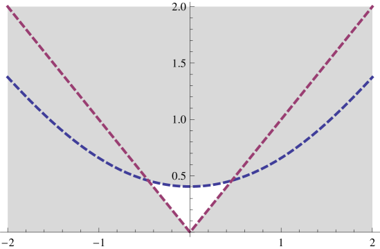
Figure 2: Phase diagram

6 Proof of Theorem 1.1

This section is devoted to the proof of Theorem 1.1. To realize it, we first show not overlapping supports of the states $\varphi_{1}$ and $\varphi_{2}$. Then we show that these states satisfy the clustering property, which yields that they are factor states, and this fact allows us to prove their non- quasi-equivalence.

6.1 Not overlapping supports of $\varphi_{1}$ and $\varphi_{2}$

As usual we put

$$e_{11}=\left(\begin{array}[]{cc}1&0\\ 0&0\end{array}\right),{\mathcal{C}}{\mathcal{C}}{\mathcal{C}}e_{22}=\left(\begin{array}[]{cc}0&0\\ 0&1\end{array}\right).$$

Now for each $n\in\mathbf{N}$, we denote

$$P_{n}:=\bigg{(}\bigotimes_{x\in\Lambda_{n}}e_{11}^{(x)}\bigg{)}\otimes{\bf 1}\!\!{\rm I},{\mathcal{C}}{\mathcal{C}}Q_{n}:=\bigg{(}\bigotimes_{x\in\Lambda_{n}}e_{22}^{(x)}\bigg{)}\otimes{\bf 1}\!\!{\rm I}.$$

Clearly, $P_{n}$ and $Q_{n}$ are orthogonal projections in $\mathcal{B}_{\Lambda_{n}}$.

Lemma 6.1.

For every $n\in{\mathbb{N}}$, one has

1. $\varphi_{1}(P_{n})=\varphi_{2}(Q_{n})=\frac{1}{2\xi_{0}}\left(\xi_{0}+\xi_{3}\right)^{2^{n}}\left(\frac{C_{1}+C_{2}+C_{3}}{4}\right)^{2^{n}-1},$

2. $\varphi_{1}(Q_{n})=\varphi_{2}(P_{n})=\frac{1}{2\xi_{0}}\left(\xi_{0}-\xi_{3}\right)^{2^{n}}\left(\frac{C_{1}+C_{2}+C_{3}}{4}\right)^{2^{n}-1}.$

Proof.

(i). From (39) we find

$$\varphi_{1}(P_{n}) = \mathrm{Tr}\big{(}\omega_{0}K_{[0,1]}\cdots K_{[n-1,n]}\mathbf{h}_{n}^{1/2}P_{n}\mathbf{h}_{n}^{1/2}K_{[n-1,n]}^{*}\cdots K_{[0,1]}^{*}\big{)}$$

$$= \mathrm{Tr}\big{(}\omega_{0}K_{[0,1]}\cdots K_{[n-1,n]}\mathbf{h}_{n}P_{n}K_{[n-1,n]}^{*}\cdots K_{[0,1]}^{*}\big{)}$$

Thanks to $he_{11}=(\xi_{0}+\xi_{3})e_{11}$ and (25) one gets

$$\mathrm{Tr}_{n-1]}(K_{[n-1,n]}\mathbf{h}_{n}P_{n}K_{[n-1,n]}^{*}) = P_{n-2}\otimes\prod_{u\in\overrightarrow{W}_{n-1}}\mathrm{Tr}_{u]}(A_{(u,(u,1),(u,2))}e_{11}^{(u)}\otimes he_{11}^{(u,1)}\otimes he_{11}^{(u,2)}A_{(u,(u,1),(u,2))})$$

$$= (\xi_{0}+\xi_{3})^{2|W_{n-1]}|}\bigg{(}\frac{C_{1}+C_{2}+C_{3}}{4}\bigg{)}^{|W_{n-1}|}P_{n-1}.$$

Hence,

$$\varphi_{1}(P_{n}) = (\xi_{0}+\xi_{3})^{|W_{n}|}\left(\frac{C_{1}+C_{2}+C_{3}}{4}\right)^{|W_{n-1}|}\mathrm{Tr}\left[\omega_{0}K_{[0,1]}\cdots K_{[n-2,n-1]}P_{n-1}K_{[n-2,n-1]}^{*}\cdots K_{[0,1]}^{*}\right]$$

.

.

.

$$= \left(\xi_{0}+\xi_{3}\right)^{|W_{n}|}\left(\frac{C_{1}+C_{2}+C_{3}}{4}\right)^{|W_{n-1}|+...+|W_{0}|}\mathrm{Tr}\left[\omega_{0}P_{0}\right]$$

$$= \left(\xi_{0}+\xi_{3}\right)^{|W_{n}|}\left(\frac{C_{1}+C_{2}+C_{3}}{4}\right)^{|\Lambda_{n-1}|}\mathrm{Tr}\left[\omega_{0}P_{0}\right]$$

$$= \frac{1}{2\xi_{0}}\left(\xi_{0}+\xi_{3}\right)^{2^{n}}\left(\frac{C_{1}+C_{2}+C_{3}}{4}\right)^{2^{n}-1}.$$

Analogously, using $h^{\prime}e_{22}=(\xi_{0}+\xi_{3})e_{22}$ we obtain

$$\mathrm{Tr}_{n-1]}(K_{[n-1,n]}\mathbf{h}^{\prime}_{n}Q_{n}K_{[n-1,n]}^{*}) = Q_{n-2}\otimes\prod_{u\in\overrightarrow{W}_{n-1}}\mathrm{Tr}_{u]}(A_{(u,(u,1),(u,2))}e_{2,2}^{(u)}\otimes h^{\prime}e_{2,2}^{(u,1)}\otimes h^{\prime}e_{22}^{(u,2)}A_{(u,(u,1),(u,2))})$$

$$= (\xi_{0}+\xi_{3})^{2|\mathcal{W}_{n-1]}|}\bigg{(}\frac{C_{1}+C_{2}+C_{3}}{4}\bigg{)}^{|\mathcal{W}_{n-1]}|}Q_{n-1}.$$

which yields

$$\varphi_{2}(Q_{n})=\frac{1}{2\xi_{0}}\left(\xi_{0}+\xi_{3}\right)^{2^{n}}\left(\frac{C_{1}+C_{2}+C_{3}}{4}\right)^{2^{n}-1}.$$

(ii) Now from $he_{22}=(\xi_{0}-\xi_{3})e_{22}$ and $h^{\prime}e_{11}=(\xi_{0}-\xi_{3})e_{11}$, we obtain

$$\mathrm{Tr}_{n-1]}K_{[n-1,n]}\mathbf{h}_{n}Q_{n}K_{[n-1,n]}^{*}=(\xi_{0}-\xi_{3})^{2|W_{n-1}|}\bigg{(}\frac{C_{1}+C_{2}+C_{3}}{4}\bigg{)}^{|W_{n-1}|}Q_{n-1}.$$

$$\mathrm{Tr}_{n-1]}K_{[n-1,n]}\mathbf{h}^{\prime}_{n}P_{n}K_{[n-1,n]}^{*}=(\xi_{0}-\xi_{3})^{2|W_{n-1}|}\bigg{(}\frac{C_{1}+C_{2}+C_{3}}{4}\bigg{)}^{|W_{n-1}|}P_{n-1}.$$

The same argument as above implies (ii). This completes the proof. ∎

Theorem 6.2.

For fixed $n\in\mathbf{N}$, one has

$$\varphi_{1}(P_{n})\rightarrow 1,{\mathcal{C}}{\mathcal{C}}\varphi_{2}(Q_{n})\rightarrow 1{\mathcal{C}}{\mathcal{C}}\textrm{as}{\mathcal{C}}{\mathcal{C}}\beta\rightarrow+\infty.$$

Proof.

We know that $\theta=\exp(2\beta)\rightarrow+\infty$ as $\beta\rightarrow+\infty$. Hence, one finds

$$\frac{1}{2\xi_{0}}=\frac{\theta^{2J_{0}}-1}{4}\sim\frac{\theta^{2J_{0}}}{4},{\mathcal{C}}{\mathcal{C}}\textrm{as}{\mathcal{C}}{\mathcal{C}}\theta\to+\infty$$

$$\left(\xi_{0}+\xi_{3}\right)^{2^{n}}=\left(\frac{2}{\theta^{2J_{0}}-1}(1+\sqrt{\frac{\theta^{2J_{0}}-\theta^{J_{0}}(\theta^{J}+\theta^{-J})+1}{\theta^{2J_{0}}-\theta^{J_{0}}(\theta^{J}+\theta^{-J})-3}})\right)^{2^{n}}\sim\left(\frac{4}{\theta^{2J_{0}}}\right)^{2^{n}},{\mathcal{C}}{\mathcal{C}}\textrm{as}{\mathcal{C}}{\mathcal{C}}\theta\to+\infty$$

$$\left(\frac{C_{1}+C_{2}+C_{3}}{4}\right)^{2^{n}-1}=\left(\frac{\theta^{2J_{0}}}{4}\right)^{2^{n}-1}.$$

Hence, we obtain

$$\varphi_{1}(P_{n})=\varphi_{2}(Q_{n})\sim\frac{\theta^{2J_{0}}}{4}\left(\frac{4}{\theta^{2J_{0}}}\right)^{2^{n}}\left(\frac{\theta^{2J_{0}}}{4}\right)^{2^{n}-1}=1.$$

So,

$$\lim_{\theta\to\infty}\varphi_{1}(P_{n})=\lim_{\theta\to\infty}\varphi_{2}(Q_{n})=1.$$

This completes the proof. ∎

Remark 6.3.

We note that from $P_{n}\leq 1-Q_{n}$ one gets

$$\lim_{\theta\to\infty}\varphi_{1}(Q_{n})=\lim_{\theta\to\infty}\varphi_{2}(P_{n})=0.$$

This implies that the states $\varphi_{1}$ and $\varphi_{2}$ have non overlapping supports.

6.2 Clustering Property for $\varphi_{1}$ and $\varphi_{2}$

In this subsection, we are going to prove that the states $\varphi_{1}$, $\varphi_{2}$ satisfy the clustering property.

Recall that a state $\varphi$ on $\mathcal{B}_{L}$ satisfies the clustering property if for every $a,f\in\mathcal{B}_{L}$ one has

$$\lim_{|g|\rightarrow\infty}\varphi(a\tau_{g}(f))=\varphi(a)\varphi(f).$$ (41)

Thanks to Theorem (5.3) there are two solutions of (14), and (15), these two solutions can be written as follows: $\big{(}\omega_{0},{\mathcal{C}}{\mathcal{C}}\{h^{(u)}=h,{\mathcal{C}}u\in L\}\big{)}$ and $\big{(}\omega_{0},\{h^{(u)}=h^{\prime},{\mathcal{C}}u\in L\}\big{)}$, where

$$\omega_{0}=\frac{1}{\xi_{0}}{\bf 1}\!\!{\rm I},~{}~{}~{}h=\xi_{0}{\bf 1}\!\!{\rm I}-\xi_{3}\sigma_{z},$$

$$\omega_{0}=\frac{1}{\xi_{0}}{\bf 1}\!\!{\rm I},~{}~{}~{}h^{\prime}=\xi_{0}{\bf 1}\!\!{\rm I}+\xi_{3}\sigma_{z}.$$

By $\varphi_{1}$, $\varphi_{2}$ we denote the corresponding backward quantum Markov chains. To prove the clustering property we need to study the following matrix:

$$A:=\begin{pmatrix}c_{1}\xi_{0}&-c_{2}\xi_{3}\\ -\frac{c_{3}}{2}\xi_{3}&\frac{c_{3}}{2}\xi_{0}\end{pmatrix}$$

One can easily prove the following fact.

Proposition 6.4.

The above given matrix $A$ is a diagonalizable matrix, and can be written as follows:

$$A:=P\begin{pmatrix}1&0\\ 0&(c_{1}-\frac{c_{3}}{2})\xi_{0}\end{pmatrix}P^{-1}$$ (42)

where

$$P:=\begin{pmatrix}\frac{c_{2}\xi_{3}}{c_{1}\xi_{0}-1}&2c_{2}\xi_{3}\\ 1&1\end{pmatrix},{\mathcal{C}}{\mathcal{C}}\det(P)=\frac{c_{2}\xi_{3}(3-2c_{1}\xi_{0})}{c_{1}\xi_{0}-1}.$$

Lemma 6.5.

Let $a\in\mathcal{B}_{\Lambda_{N_{0}}}$, for some $N_{0}\in{\mathbb{N}}$, and $f_{n}=\bigotimes\limits_{x\in W_{n}}f^{(x)}=f^{x_{W_{n}}^{(1)}}\otimes{\bf 1}\!\!{\rm I}_{W_{n}\setminus\{x_{W_{n}}^{(1)}\}}\in\mathcal{B}_{W_{n}}$, where $f^{x_{W_{n}}^{(1)}}=f$, then for each backward quantum Markov chains $\varphi_{1}$, $\varphi_{2}$ we have

$$\lim_{n\rightarrow\infty}\varphi_{k}(a\otimes{\bf 1}\!\!{\rm I}\cdots\otimes{\bf 1}\!\!{\rm I}\otimes f_{n})=\varphi_{k}(a)\varphi_{k}(f),{\mathcal{C}}{\mathcal{C}}k=1,2.$$

Proof.

By symmetry of calculations, it is enough to prove the result for $\big{(}\omega_{0},{\mathcal{C}}{\mathcal{C}}\{h^{(u)}=h,{\mathcal{C}}u\in L\}\big{)}$. From (12) and (16) we have:

$$\varphi^{(n)}_{w_{0},\mathbf{h}}(a_{N_{0}}\otimes{\bf 1}\!\!{\rm I}\cdots\otimes{\bf 1}\!\!{\rm I}\otimes f)={\rm Tr}(\omega_{0}\mathcal{E}_{0}\circ\cdots\circ\mathcal{E}_{N_{0}}(a\otimes\mathcal{E}_{N_{0}+1}({\bf 1}\!\!{\rm I}\otimes\cdots\otimes\mathcal{E}_{n-1}({\bf 1}\!\!{\rm I}\otimes\hat{\mathcal{E}}_{n}({\bf 1}\!\!{\rm I}\otimes f))\cdots))$$

First, let us calculate $\hat{\mathcal{E}}_{n}({\bf 1}\!\!{\rm I}\otimes f)$. From (16) it follows that

$$\hat{\mathcal{E}}_{n}(f\otimes{\bf 1}\!\!{\rm I}) = \bigotimes\limits_{x\in W_{n}}{\rm Tr}_{x]}(A_{x\vee S(x)}f^{(x)}\otimes h_{S(x)}A^{*}_{x\vee S(x)})$$

$$= {\rm Tr}_{x_{W_{n}}^{(1)}]}(A_{x_{W_{n}}^{(1)}\vee S(x_{W_{n}}^{(1)})}f^{(x_{W_{n}}^{(1)})}\otimes h_{S(x_{W_{n}}^{(1)})}A^{*}_{x_{W_{n}}^{(1)}\vee S(x_{W_{n}}^{(1)})})\otimes$$

$$\bigotimes\limits_{x\in W_{n}\setminus\{x_{W_{n}}^{(1)}\}}{\rm Tr}_{x]}(A_{x\vee S(x)}h_{S(x)}A^{*}_{x\vee S(x)})$$

$$= \bigg{(}\alpha_{1}f^{(x_{W_{n}}^{(1)})}+\alpha_{2}(f^{(x_{W_{n}}^{(1)})}\sigma_{z}^{(x_{W_{n}}^{(1)})}+\sigma_{z}^{(x_{W_{n}}^{(1)})}f^{(x_{W_{n}}^{(1)})})$$

$$+\alpha_{3}\sigma_{z}^{(x_{W_{n}}^{(1)})}f^{(x_{W_{n}}^{(1)})}\sigma_{z}^{(x_{W_{n}}^{(1)})}\bigg{)}\otimes\bigotimes\limits_{x\in W_{n}\setminus\{x_{W_{n}}^{(1)}\}}h_{x}$$

$$= g^{(x_{W_{n}}^{(1)})}\otimes\bigotimes\limits_{x\in W_{n}\setminus\{x_{W_{n}}^{(1)}\}}h_{x},$$

where

$$g^{(x_{W_{n}}^{(1)})}=\alpha_{1}f^{(x_{W_{n}}^{(1)})}+\alpha_{2}(f_{1}^{(x_{W_{n}}^{(1)})}\sigma_{z}^{(x_{W_{n}}^{(1)})}+\sigma_{z}^{(x_{W_{n}}^{(1)})}f^{(x_{W_{n}}^{(1)})})+\alpha_{3}\sigma_{z}^{(x_{W_{n}}^{(1)})}f^{(x_{W_{n}}^{(1)})}\sigma_{z}^{(x_{W_{n}}^{(1)})},$$

and

$$\left\{\begin{array}[]{ll}\alpha_{1}=(C_{1}-2\delta_{1}^{2})\xi_{0}^{2}+(C_{2}-2\delta_{1}^{2})\xi_{3}^{2}\\ \alpha_{2}=-\frac{C_{3}}{2}\xi_{0}\xi_{3}\\ \alpha_{3}=2\delta_{1}^{2}(\xi_{0}^{2}+\xi_{3}^{2})\end{array}\right..$$

Hence, one has

$$\mathcal{E}_{n-1}({\bf 1}\!\!{\rm I}\otimes\hat{\mathcal{E}}_{n}(f\otimes{\bf 1}\!\!{\rm I})) = {\rm Tr}_{x_{W_{n-1}}^{(1)}]}(A_{x_{W_{n-1}}^{(1)}\vee S(x_{W_{n-1}}^{(1)})}{\bf 1}\!\!{\rm I}\otimes g^{(x_{W_{n}}^{(1)})}\otimes hA^{*}_{x_{W_{n-1}}^{(1)}\vee S(x_{W_{n-1}}^{(1)})})\otimes$$

$$\bigotimes\limits_{x\in W_{n-1}\setminus\{x_{W_{n-1}}^{(1)}\}}h_{(x)}$$

$$= (\alpha_{1,g}{\bf 1}\!\!{\rm I}^{(x_{W_{n-1}}^{(1)})}+\alpha_{2,g}\sigma_{z}^{(x_{W_{n-1}}^{(1)})})\otimes\bigotimes\limits_{x\in W_{n-1}\setminus\{x_{W_{n-1}}^{(1)}\}}h_{(x)}$$

$$= \alpha_{1,g}{\bf 1}\!\!{\rm I}^{(x_{W_{n-1}}^{(1)})}\otimes\bigotimes\limits_{x\in W_{n-1}\setminus\{x_{W_{n-1}}^{(1)}\}}h_{(x)}$$

$$+\alpha_{2,g}\sigma_{z}^{(x_{W_{n-1}}^{(1)})}\otimes\bigotimes\limits_{x\in W_{n-1}\setminus\{x_{W_{n-1}}^{(1)}\}}h_{(x)}$$

So, one finds

$$\mathcal{E}_{n-1}({\bf 1}\!\!{\rm I}\otimes\hat{\mathcal{E}}_{n}(f\otimes{\bf 1}\!\!{\rm I})) = v_{1}{\bf 1}\!\!{\rm I}^{(x_{W_{n-1}}^{(1)})}\otimes\bigotimes\limits_{x\in W_{n-1}\setminus\{x_{W_{n-1}}^{(1)}\}}h_{(x)}+v^{{}^{\prime}}_{1}\sigma_{z}^{(x_{W_{n-1}}^{(1)})}\otimes\bigotimes\limits_{x\in W_{n-1}\setminus\{x_{W_{n-1}}^{(1)}\}}h_{(x)}$$

where

$$\left\{\begin{array}[]{ll}\alpha_{1,X}=C_{1}{\rm Tr}(X)\xi_{0}-C_{2}{\rm Tr}(\sigma_{z}X)\xi_{3}\\ \alpha_{2,X}=\frac{C_{3}}{2}\left({\rm Tr}(\sigma_{z}X)\xi_{0}-{\rm Tr}(X)\xi_{3}\right)\\ v_{1}=\alpha_{1,g}\\ v_{1}^{{}^{\prime}}=\alpha_{2,g}\\ \end{array}\right.$$

Then by iteration we obtain

$$\mathcal{E}_{n-k}({\bf 1}\!\!{\rm I}\otimes...\mathcal{E}_{n-1}({\bf 1}\!\!{\rm I}\otimes\hat{\mathcal{E}}_{n}(f\otimes{\bf 1}\!\!{\rm I}))) = v_{k}{\bf 1}\!\!{\rm I}^{(x_{W_{n-1}}^{(1)})}\otimes\bigotimes\limits_{x\in W_{n-1}\setminus\{x_{W_{n-1}}^{(1)}\}}h_{(x)}$$

$$+v^{{}^{\prime}}_{k}\sigma_{z}^{(x_{W_{n-1}}^{(1)})}\otimes\bigotimes\limits_{x\in W_{n-1}\setminus\{x_{W_{n-1}}^{(1)}\}}h_{(x)}$$

where

$$\left\{\begin{array}[]{ll}v_{k}=v_{k-1}C_{1}\xi_{0}-C_{2}\xi_{3}v_{k-1}^{{}^{\prime}}\\ v_{k}^{{}^{\prime}}=-\frac{C_{3}}{2}\xi_{3}v_{k-1}+\frac{C_{3}}{2}\xi_{0}v_{k-1}^{{}^{\prime}}\\ \end{array}\right.$$

Now let calculate the explicit form of the sequence $v_{k}$, we can see :

$$\begin{pmatrix}v_{k}\\ v_{k}^{{}^{\prime}}\end{pmatrix} = A\begin{pmatrix}v_{k-1}\\ v_{k-1}^{{}^{\prime}}\end{pmatrix}$$

$$\vdots$$

$$= A^{k-1}\begin{pmatrix}v_{1}\\ v_{1}^{{}^{\prime}}\end{pmatrix}$$

Then by (42) we get,

$$\begin{pmatrix}v_{k}\\ v_{k}^{{}^{\prime}}\end{pmatrix} = P\begin{pmatrix}1&0\\ 0&(c_{1}-\frac{c_{3}}{2})^{k-1}\xi_{0}^{k-1}\end{pmatrix}P^{-1}\begin{pmatrix}v_{1}\\ v_{1}^{{}^{\prime}}\end{pmatrix}$$

$$= \begin{pmatrix}\frac{1}{3-2c_{1}\xi_{0}}+\frac{2\xi_{0}^{k-1}(c_{1}-\frac{c_{3}}{2})^{k-1}(1-c_{1}\xi_{0})}{3-2c_{1}\xi_{0}}&-\frac{2c_{2}\xi_{3}}{3-2c_{1}\xi_{0}}+\frac{2c_{2}\xi_{3}\xi_{0}^{k-1}(c_{1}-\frac{c_{3}}{2})^{k-1}}{3-2c_{1}\xi_{0}}\\[5.69054pt] \frac{c_{1}\xi_{0}-1}{c_{2}\xi_{3}(3-2c_{1}\xi_{0})}+\frac{\xi_{0}^{k-1}(c_{1}-\frac{c_{3}}{2})^{k-1}(1-c_{1}\xi_{0})}{c_{2}\xi_{3}(3-2c_{1}\xi_{0})}&\frac{-2(c_{1}\xi_{0}-1)}{3-2c_{1}\xi_{0}}+\frac{\xi_{0}^{k-1}(c_{1}-\frac{c_{3}}{2})^{k-1}}{3-2c_{1}\xi_{0}}\end{pmatrix}\begin{pmatrix}v_{1}\\[5.69054pt] v_{1}^{{}^{\prime}}\end{pmatrix}$$

$$= \begin{pmatrix}\eta_{1}+\widehat{\eta_{1}}\xi_{0}^{k-1}(c_{1}-\frac{c_{3}}{2})^{k-1}&\eta_{2}-\eta_{2}\xi_{0}^{k-1}(c_{1}-\frac{c_{3}}{2})^{k-1}\\[5.69054pt] \widehat{\eta_{2}}-\widehat{\eta_{2}}\xi_{0}^{k-1}(c_{1}-\frac{c_{3}}{2})^{k-1}&\widehat{\eta_{1}}+\eta_{1}\xi_{0}^{k-1}(c_{1}-\frac{c_{3}}{2})^{k-1}\end{pmatrix}\begin{pmatrix}v_{1}\\[5.69054pt] v_{1}^{{}^{\prime}}\\ \end{pmatrix}$$

where

$$\eta_{1}=\frac{1}{3-2c_{1}\xi_{0}},{\mathcal{C}}{\mathcal{C}}\widehat{\eta_{1}}=\frac{2(1-c_{1}\xi_{0})}{3-2c_{1}\xi_{0}}$$

$$\eta_{2}=-\frac{2c_{2}\xi_{3}}{3-2c_{1}\xi_{0}},{\mathcal{C}}{\mathcal{C}}\widehat{\eta_{2}}=\frac{c_{1}\xi_{0}-1}{c_{2}\xi_{3}(3-2c_{1}\xi_{0})}$$

Hence,

$$\left\{\begin{array}[]{ll}v_{k}=\left(\eta_{1}+\widehat{\eta_{1}}\xi_{0}^{k-1}(c_{1}-\frac{c_{3}}{2})^{k-1}\right)v_{1}+\left(\eta_{2}-\eta_{2}\xi_{0}^{k-1}(c_{1}-\frac{c_{3}}{2})^{k-1}\right)v_{1}^{{}^{\prime}}\\[5.69054pt] v_{k}^{{}^{\prime}}=\left(\widehat{\eta_{2}}-\widehat{\eta_{2}}\xi_{0}^{k-1}(c_{1}-\frac{c_{3}}{2})^{k-1}\right)v_{1}+\left(\widehat{\eta_{1}}+\eta_{1}\xi_{0}^{k-1}(c_{1}-\frac{c_{3}}{2})^{k-1}\right)v_{1}^{{}^{\prime}}\\ \end{array}\right.$$

So, one finds

$$\varphi^{(n)}_{w_{0},\mathbf{h}}(a\otimes{\bf 1}\!\!{\rm I}\cdots\otimes{\bf 1}\!\!{\rm I}\otimes f)=v_{n-N_{0}+1}{\rm Tr}\left(\omega_{0}\mathcal{E}_{0}\circ\cdots\circ\mathcal{E}_{N_{0}}\bigg{(}a\otimes{\bf 1}\!\!{\rm I}^{(x_{W_{N_{0}+1}})}\otimes\bigotimes\limits_{x\in W_{N_{0}+1}\setminus\{x_{W_{N_{0}+1}}^{(1)}\}}h_{x}\bigg{)}\right)$$

$$+v_{n-N_{0}+1}^{{}^{\prime}}{\rm Tr}\left(\omega_{0}\mathcal{E}_{0}\circ\cdots\circ\mathcal{E}_{N_{0}}\bigg{(}a\otimes\sigma_{z}^{(x_{W_{N_{0}+1}})}\otimes\bigotimes\limits_{x\in W_{N_{0}+1}\setminus\{x_{W_{N_{0}+1}}^{(1)}\}}h_{x}\bigg{)}\right)$$

$$=\left(\eta_{1}+\widehat{\eta_{1}}\xi_{0}^{n-N_{0}}(c_{1}-\frac{c_{3}}{2})^{n-N_{0}}\right)v_{1}{\rm Tr}\left(\omega_{0}\mathcal{E}_{0}\circ\cdots\circ\mathcal{E}_{N_{0}}\bigg{(}a\otimes{\bf 1}\!\!{\rm I}^{(x_{W_{N_{0}+1}})}\otimes\bigotimes\limits_{x\in W_{N_{0}+1}\setminus\{x_{W_{N_{0}+1}}^{(1)}\}}h_{x}\bigg{)}\right)$$

$$+\left(\eta_{2}-\eta_{2}\xi_{0}^{n-N_{0}}(c_{1}-\frac{c_{3}}{2})^{n-N_{0}}\right)v_{1}^{{}^{\prime}}{\rm Tr}\left(\omega_{0}\mathcal{E}_{0}\circ\cdots\circ\mathcal{E}_{N_{0}}\bigg{(}a\otimes{\bf 1}\!\!{\rm I}^{(x_{W_{N_{0}+1}})}\otimes\bigotimes\limits_{x\in W_{N_{0}+1}\setminus\{x_{W_{N_{0}+1}}^{(1)}\}}h_{x}\bigg{)}\right)$$

$$+\left(\widehat{\eta_{2}}-\widehat{\eta_{2}}\xi_{0}^{n-N_{0}}(c_{1}-\frac{c_{3}}{2})^{k-1}\right)v_{1}{\rm Tr}\left(\omega_{0}\mathcal{E}_{0}\circ\cdots\circ\mathcal{E}_{N_{0}}\bigg{(}a\otimes\sigma_{z}^{(x_{W_{N_{0}+1}})}\otimes\bigotimes\limits_{x\in W_{N_{0}+1}\setminus\{x_{W_{N_{0}+1}}^{(1)}\}}h_{x}\bigg{)}\right)$$

$$+\left(\widehat{\eta_{1}}+\eta_{1}\xi_{0}^{n-N_{0}}(c_{1}-\frac{c_{3}}{2})^{n-N_{0}}\right)v_{1}^{{}^{\prime}}{\rm Tr}\left(\omega_{0}\mathcal{E}_{0}\circ\cdots\circ\mathcal{E}_{N_{0}}\bigg{(}a\otimes\sigma_{z}^{(x_{W_{N_{0}+1}})}\otimes\bigotimes\limits_{x\in W_{N_{0}+1}\setminus\{x_{W_{N_{0}+1}}^{(1)}\}}h_{x}\bigg{)}\right)$$

One can see that $\xi_{0}^{n-N_{0}}\rightarrow 0$, as $n\rightarrow\infty$, which implies

$$\lim_{n\rightarrow\infty}\varphi_{w_{0},\mathbf{h}}(a\otimes{\bf 1}\!\!{\rm I}\otimes\cdots\otimes{\bf 1}\!\!{\rm I}\otimes f_{n})=(\eta_{1}v_{1}+\eta_{2}v_{1}^{{}^{\prime}}){\rm Tr}\bigg{(}\omega_{0}\mathcal{E}_{0}\circ\cdots\circ\mathcal{E}_{N_{0}}(a\otimes{\bf 1}\!\!{\rm I}^{(x_{W_{N_{0}+1}})}\otimes$$

$$\bigotimes\limits_{x\in W_{N_{0}+1}\setminus\{x_{W_{N_{0}+1}}^{(1)}\}}h_{x})\bigg{)}$$

$$+(\widehat{\eta_{2}}v_{1}+\widehat{\eta_{1}}v_{1}^{{}^{\prime}}){\rm Tr}\left(\omega_{0}\mathcal{E}_{0}\circ\cdots\circ\mathcal{E}_{N_{0}}(a\otimes\sigma_{z}^{(x_{W_{N_{0}+1}})}\otimes\bigotimes\limits_{x\in W_{N_{0}+1}\setminus\{x_{W_{N_{0}+1}}^{(1)}\}}h_{x})\right)$$

where

$$\left\{\begin{array}[]{ll}\eta_{1}v_{1}+\eta_{2}v_{1}^{{}^{\prime}}=\frac{\xi_{0}^{2}}{6-4C_{1}\xi_{0}}[(4C_{3}-2C_{1}){\rm Tr}(f)-\sqrt{\Delta(\theta)}(4C_{2}+C_{3}){\rm Tr}(\sigma_{z}f)]\\[5.69054pt] \widehat{\eta_{2}}v_{1}+\widehat{\eta_{1}}v_{1}^{{}^{\prime}}=-c_{3}\xi_{3}(\eta_{1}v_{1}+\eta_{2}v_{1}^{{}^{\prime}})\\ \end{array}\right.$$

On other hand we have

$$\varphi_{w_{0},\mathbf{h}}(f)=C_{3}(\eta_{1}v_{1}+\eta_{2}v_{1}^{{}^{\prime}}),$$

Hence, one gets

$$\lim_{n\rightarrow\infty}\varphi_{w_{0},\mathbf{h}}(a\otimes\cdots\otimes f_{n}) = \varphi_{w_{0},\mathbf{h}}(f){\rm Tr}\bigg{(}\omega_{0}\mathcal{E}_{0}\circ\cdots\circ\mathcal{E}_{N_{0}}(a\otimes h^{(x_{W_{N_{0}+1}})}\otimes\bigotimes\limits_{x\in W_{N_{0}+1}\setminus\{x_{W_{N_{0}+1}}^{(1)}\}}h_{x}\bigg{)}$$

$$= \varphi_{w_{0},\mathbf{h}}(f){\rm Tr}\left(\omega_{0}\mathcal{E}_{0}\circ\cdots\circ\hat{\mathcal{E}}_{N_{0}}(a)\right)$$

$$= \varphi_{w_{0},\mathbf{h}}(f)\varphi_{w_{0},\mathbf{h}}(a).$$

This completes the prove. ∎

Now we are ready to prove the clustering property.

Theorem 6.6.

The states $\varphi_{1}$ and $\varphi_{2}$ satisfy the clustering property.

Proof.

Thanks to the density argument, without lost of generality, we may assume $a,f\in\mathcal{B}_{loc}$. This means that there are $N_{0},m_{0}\in{\mathbb{N}}$ such that $a\in\mathcal{B}_{\Lambda_{N_{0}}}$, $f\in\mathcal{B}_{\Lambda_{m_{0}}}$. Moreover, $f$ can be write in the following form

$$f=\bigotimes\limits_{x\in\Lambda_{m_{0}}}f^{(x)}.$$

By symmetry of calculations, it is enough to prove the result for $\big{(}\omega_{0},{\mathcal{C}}{\mathcal{C}}\{h^{(u)}=h,{\mathcal{C}}u\in L\}\big{)}$.
In what follows, we assume that $g\in W_{n}$. Therefore, we put $g_{n}:=g$. Then one has

$$\tau_{g_{n}}(f) = \bigotimes\limits_{x\in\Lambda_{m_{0}}}f^{(g_{n}\circ x)}$$

$$= f^{(g_{n})}\otimes f^{(g_{n},W_{1})}\otimes f^{(g_{n},W_{2})}\otimes...\otimes f^{(g_{n},W_{m_{0}})},$$

where

$$f^{(g_{n},W_{k})}=\bigotimes\limits_{x\in W_{k}}f^{(g_{n}\circ x)}{\mathcal{C}}{\mathcal{C}}\text{and}{\mathcal{C}}{\mathcal{C}}\{g_{n},W_{k}\}=\{(g_{n}\circ x),{\mathcal{C}}{\mathcal{C}}x\in W_{k}\}.$$

We can see $\tau_{g_{n}}(f)$ as an element of $B_{\Lambda_{n+m_{0}}}$, i.e.

$$\tau_{g_{n}}(f) = {\bf 1}\!\!{\rm I}_{\Lambda_{n-1}}\otimes(f^{(g_{n})}\otimes{\bf 1}\!\!{\rm I}_{W_{n}\setminus\{g_{n}\}})\otimes(f^{(g_{n},W_{1})}\otimes{\bf 1}\!\!{\rm I}_{W_{n+1}\setminus\{g_{n},W_{1}\}})\otimes$$

$$...\otimes(f^{(g_{n},W_{m_{0}})}\otimes{\bf 1}\!\!{\rm I}_{W_{n+m_{0}}\setminus\{g_{n},W_{m_{0}}\}}).$$

For the sake of simplicity, let us denote

$$\tau_{g_{n}}(f) = \bigotimes\limits_{x\in\Lambda_{n+m_{0}}}f_{1}^{(x)}.$$

From (12) and (16) it follows that

$$\varphi_{w_{0},\mathbf{h}}(a\otimes{\bf 1}\!\!{\rm I}\otimes\cdots\otimes{\bf 1}\!\!{\rm I}\otimes\tau_{g_{n}}(f))=\varphi^{(n+m_{0})}_{w_{0},\mathbf{h}}(a\otimes{\bf 1}\!\!{\rm I}\cdots\otimes{\bf 1}\!\!{\rm I}\otimes\tau_{g_{n}}(f))$$

$$={\rm Tr}(\omega_{0}\mathcal{E}_{0}\circ\cdots\circ\mathcal{E}_{N_{0}}(a\otimes\mathcal{E}_{N_{0}+1}({\bf 1}\!\!{\rm I}\otimes\cdots\otimes\mathcal{E}_{n+m_{0}-1}({\bf 1}\!\!{\rm I}\otimes\hat{\mathcal{E}}_{n+m_{0}}(\tau_{g_{n}}(f)))...)).$$

Let us calculate $\hat{\mathcal{E}}_{n+m_{0}}(\tau_{g_{n}}(f))$. Indeed, from (16) one gets

$$\hat{\mathcal{E}}_{n+m_{0}}(\tau_{g_{n}}(f)\otimes h_{W_{n+m_{0}+1}}) = {\rm Tr}_{n+m_{0}]}(K_{[n+m_{0},n+m_{0}+1]}\tau_{g_{n}}(f)\otimes h_{W_{n+m_{0}+1}}K_{[n+m_{0},n+m_{0}+1]}^{*})$$

$$= \bigotimes\limits_{x\in\Lambda_{n+m_{0}-1}}f_{1}^{(x)}\bigotimes\limits_{x\in W_{n+m_{0}}}{\rm Tr}_{x]}(A_{x\vee S(x)}f_{1}^{(x)}\otimes h^{(S(x))}A^{*}_{x\vee S(x)})$$

$$= \bigotimes\limits_{x\in\Lambda_{n+m_{0}-1}}f_{1}^{(x)}\bigotimes\limits_{x\in W_{m_{0}}}{\rm Tr}_{g_{n}\circ x]}(A_{g_{n}\circ x\vee S(g_{n}\circ x)}f^{(g_{n}\circ x)}\otimes h^{(S(g_{n}\circ x))}A^{*}_{g_{n}\circ x\vee S(g_{n}\circ x)})$$

$$\otimes\bigotimes\limits_{x\in W_{n+m_{0}}\setminus\{g_{n},W_{m_{0}}\}}{\rm Tr}_{x]}(A_{x\vee S(x)}h^{(x)}A^{*}_{x\vee S(x)})$$

$$= \bigotimes\limits_{x\in\Lambda_{n+m_{0}-1}}f_{1}^{(x)}\bigotimes\limits_{x\in W_{m_{0}}}T_{m_{0}}^{(g_{n}\circ x)}\otimes\bigotimes\limits_{x\in W_{n+m_{0}}\setminus\{g_{n},W_{m_{0}}\}}h^{(x)}$$

where

$$T_{m_{0}}^{(g_{n}\circ x)}={\rm Tr}_{g_{n}\circ x]}(A_{(g_{n}\circ x)\vee S(g_{n}\circ x)}f^{(g_{n}\circ x)}\otimes h^{(S(g_{n}\circ x))}A^{*}_{(g_{n}\circ x)\vee S(g_{n}\circ x)}).$$

Hence,

$$\mathcal{E}_{n+m_{0}-1}({\bf 1}\!\!{\rm I}\otimes\hat{\mathcal{E}}_{n+m_{0}}(\tau_{g_{n}}(f))) = \bigotimes\limits_{x\in\Lambda_{n+m_{0}-2}}f_{1}^{(x)}{\rm Tr}_{n+m_{0}-1]}(K_{[n+m_{0}-1,n+m_{0}]}\bigotimes\limits_{x\in W_{n+m_{0}-1}}f_{1}^{(x)}\bigotimes\limits_{x\in W_{m_{0}}}T_{m_{0}}^{(g_{n}\circ x)}$$

$$\otimes\bigotimes\limits_{x\in W_{n+m_{0}}\setminus\{g_{n},W_{m_{0}}\}}h^{(x)}K_{[n+m_{0}-1,n+m_{0}]}^{*})$$

$$= \bigotimes\limits_{x\in\Lambda_{n+m_{0}-2}}f_{1}^{(x)}\bigotimes\limits_{x\in W_{m_{0}-1}}{\rm Tr}_{g_{n}\circ x]}\bigg{(}A_{(g_{n}\circ x)\vee S(g_{n}\circ x)}f^{(g_{n}\circ x)}$$

$$\otimes T_{m_{0}}^{(S(g_{n}\circ x))}\otimes A^{*}_{(g_{n}\circ x)\vee S(g_{n}\circ x)}\bigg{)}$$

$$\otimes\bigotimes\limits_{x\in W_{n+m_{0}-1}\setminus\{g_{n},W_{m_{0}-1}\}}{\rm Tr}_{x]}(A_{x\vee S(x)}h^{(x)}A^{*}_{x\vee S(x)})$$

$$= \bigotimes\limits_{x\in\Lambda_{n+m_{0}-2}}f_{1}^{(x)}\bigotimes\limits_{x\in W_{m_{0}-1}}T_{m_{0}-1}^{(g_{n}\circ x)}\otimes\bigotimes\limits_{x\in W_{n+m_{0}-1}\setminus\{g_{n},W_{m_{0}}\}}h^{(x)}$$

where

$$T_{m_{0}-1}^{(g_{n}\circ x)}={\rm Tr}_{g_{n}\circ x]}\left(A_{g_{n}\circ x\vee S(g_{n}\circ x)}f^{(g_{n}\circ x)}\otimes T_{m_{0}}^{(S(g_{n}\circ x))}\otimes A^{*}_{g_{n}\circ x\vee S(g_{n}\circ x)}\right).$$

By iteration, we obtain

$$\mathcal{E}_{n}({\bf 1}\!\!{\rm I}\otimes\mathcal{E}_{n+1}({\bf 1}\!\!{\rm I}\otimes...\otimes\mathcal{E}_{n+m_{0}-1}({\bf 1}\!\!{\rm I}\otimes\hat{\mathcal{E}}_{n+m_{0}}(\tau_{g_{n}}(f)))...)) = \bigotimes\limits_{x\in W_{0}}T_{0}^{(g_{n}\circ x)}\otimes\bigotimes\limits_{x\in W_{n}\setminus\{g_{n},W_{0}\}}h^{(x)}$$

$$= T_{0}^{(g_{n}\circ x_{0})}\otimes\bigotimes\limits_{x\in W_{n}\setminus\{g_{n}\circ x_{0}\}}h^{(x)},$$

which yields

$$\varphi_{w_{0},\mathbf{h}}(a_{N_{0}}\otimes{\bf 1}\!\!{\rm I}\otimes{\bf 1}\!\!{\rm I}...\otimes{\bf 1}\!\!{\rm I}\otimes\tau_{g_{n}}(f)) = {\rm Tr}(\omega_{0}\mathcal{E}_{0}\circ...\circ\mathcal{E}_{N_{0}}(a_{N_{0}}\otimes\mathcal{E}_{N_{0}+1}({\bf 1}\!\!{\rm I}$$

$$\otimes\mathcal{E}_{N_{0}+2}({\bf 1}\!\!{\rm I}\otimes...\otimes\mathcal{E}_{n-1}(T_{0}^{(g_{n}\circ x_{0})}\otimes\bigotimes\limits_{x\in W_{n}\setminus\{g_{n}\circ x_{0}\}}h^{(x)}))).$$

Then Lemma 6.5 implies

$$\lim_{n\rightarrow\infty}\varphi_{w_{0},\mathbf{h}}(a_{N_{0}}\otimes{\bf 1}\!\!{\rm I}\otimes{\bf 1}\!\!{\rm I}...\otimes{\bf 1}\!\!{\rm I}\otimes\tau_{g_{n}}(f)) = \varphi_{w_{0},\mathbf{h}}(a_{N_{0}}){\rm Tr}(\omega_{0}\mathcal{E}_{0}\circ...\circ\mathcal{E}_{n-1}(T_{0}^{(g_{n}\circ x_{0})}\otimes\bigotimes\limits_{x\in W_{n}\setminus\{g_{n}\circ x_{0}\}}h^{(x)})))$$

$$= \varphi_{w_{0},\mathbf{h}}(a_{N_{0}})\varphi_{w_{0},\mathbf{h}}(\tau_{g_{n}}(f)).$$

This completes the proof. ∎

6.3 Non quasi equivalence of $\varphi_{1}$ and $\varphi_{2}$

In this subsection we are going to prove that the states $\varphi_{1}$ and $\varphi_{2}$ are not quasi equivalent. To establish the non-quasi equivalence, we are going to use the following result (see [18, Corollary 2.6.11]).

Theorem 6.7.

Let $\varphi_{1},$ $\varphi_{2}$ be two factor states on a quasi-local algebra ${\mathfrak{A}}=\cup_{\Lambda}{\mathfrak{A}}_{\Lambda}$. The states $\varphi_{1},$ $\varphi_{2}$ are quasi-equivalent if and only if for any given $\varepsilon>0$ there exists a finite volume $\Lambda\subset L$ such that $\|\varphi_{1}(a)-\varphi_{2}(a)\|<\varepsilon\|a\|$ for all $a\in B_{\Lambda^{{}^{\prime}}}$ with $\Lambda^{{}^{\prime}}\cap\Lambda=\emptyset.$

Now due to Theorem 6.6 the states $\varphi_{1}$ and $\varphi_{2}$ have clustering property, and hence they are factor states. Let us define an element of $\mathcal{B}_{\Lambda_{n}}$ as follows:

$$E_{\Lambda_{n}}:=e_{11}^{x_{W_{n}}^{(1)}}\otimes\bigg{(}\bigotimes_{y\in\Lambda_{n}\setminus\{x_{W_{n}}^{(1)}\}}{\bf 1}\!\!{\rm I}^{y}\bigg{)},$$

where $x_{W_{n}}^{(1)}$ is defined in (6). Now we are going to calculate $\varphi_{1}(E_{\Lambda_{n}})$ and $\varphi_{2}(E_{\Lambda_{n}})$, respectively. First consider the state $\varphi_{1}$, then we know that this state is defined by $\omega_{0}=\frac{1}{\xi_{0}}{\bf 1}\!\!{\rm I}$ and $h^{x}=h=\xi_{0}{\bf 1}\!\!{\rm I}+\xi_{3}\sigma_{z}$. Define two elements of $\mathcal{B}_{W_{n}}$ by

$$\hat{\mathbf{h}}_{n}:={\bf 1}\!\!{\rm I}^{x_{W_{n}}^{(1)}}\otimes\bigotimes_{x\in W_{n}\setminus\{x_{W_{n}}^{(1)}\}}h^{(x)}$$

$$\check{\mathbf{h}}_{n}:=\sigma_{z}^{x_{W_{n}}^{(1)}}\otimes\bigotimes_{x\in W_{n}\setminus\{x_{W_{n}}^{(1)}\}}h^{(x)}$$

Lemma 6.8.

Let

$$\hat{\psi}_{n}:=\mathrm{Tr}_{n-1]}\big{[}\omega_{0}K_{[0,1]}\cdots K_{[n-1,n]}\hat{\mathbf{h}}_{n}K_{[n-1,n]}^{*}\cdots K_{[0,1]}^{*}\big{]}$$

$$\check{\psi}_{n}:=\mathrm{Tr}_{n-1]}\big{[}\omega_{0}K_{[0,1]}\cdots K_{[n-1,n]}\check{\mathbf{h}}_{n}K_{[n-1,n]}^{*}\cdots K_{[0,1]}^{*}\big{]}$$

Then there are two pairs of reals $(\hat{\rho}_{1},\hat{\rho}_{2})$ and $(\check{\rho}_{1},\check{\rho}_{2})$ depending on $\theta$ such that

$$\left\{\begin{array}[]{ll}\hat{\psi}_{n}=\hat{\rho}_{1}+\hat{\rho}_{2}(\frac{C_{1}}{C_{3}}-1)^{n},\\ \\ \check{\psi}_{n}=\check{\rho}_{1}+\check{\rho}_{2}(\frac{C_{1}}{C_{3}}-1)^{n}\\ \end{array}\right.$$

Proof.

One can see that

$$\left(\begin{array}[]{ll}\hat{\psi}_{n}\\ \\ \check{\psi}_{n}\end{array}\right) = \left(\begin{array}[]{c}\mathrm{Tr}_{n-1]}\big{[}\omega_{0}K_{[0,1]}\cdots K_{[n-2,n-1]}\mathrm{Tr}_{n-1]}[K_{[n-1,n]}\hat{\mathbf{h}}_{n}K_{[n-1,n]}^{*}]K_{[n-2,n-1]}^{*}\cdots K_{[0,1]}^{*}\big{]},\\ \\ \mathrm{Tr}_{n-1]}\big{[}\omega_{0}K_{[0,1]}\cdots K_{[n-2,n-1]}Tr_{n-1]}[K_{[n-1,n]}\check{\mathbf{h}}_{n}K_{[n-1,n]}^{*}]K_{[n-2,n-1]}^{*}\cdots K_{[0,1]}^{*}\big{]}\end{array}\right).$$

After small calculations, we find

$$\left\{\begin{array}[]{ll}\mathrm{Tr}_{x]}\left[A_{(x,(x,1),(x,2))}\big{(}{\bf 1}\!\!{\rm I}^{(x)}\otimes{\bf 1}\!\!{\rm I}^{(x,1)}\otimes h^{(x,2)}\big{)}A_{(x,(x,1),(x,2))}\right]=C_{1}\xi_{0}{\bf 1}\!\!{\rm I}^{(x)}+\frac{1}{2}C_{3}\xi_{3}\sigma_{z}^{(x)}\\ \\ \mathrm{Tr}_{x]}\big{[}A_{(x,(x,1),(x,2))}\big{(}{\bf 1}\!\!{\rm I}^{(x)}\otimes\sigma^{(x,1)}\otimes h_{(\xi_{0},\xi_{3})}^{(x,2)}\big{)}A_{(x,(x,1),(x,2))}\big{]}=C_{2}\xi_{3}{\bf 1}\!\!{\rm I}^{(x)}+\frac{1}{2}\sigma_{z}^{(x)}\end{array}\right.$$

Hence, one gets

$$\left\{\begin{array}[]{ll}\mathrm{Tr}_{n-1]}K_{[n-1,n]}\hat{\mathbf{h}}_{n}K_{[n-1,n]}^{*}=C_{1}\xi_{0}\hat{h}_{n-1}+\frac{1}{2}C_{3}\xi_{3}\check{h}_{n-1},\\ \\ \mathrm{Tr}_{n-1]}K_{[n-1,n]}\check{\mathbf{h}}_{n}K_{[n-1,n]}^{*}=C_{2}\xi_{3}\hat{h}_{n-1}+\frac{1}{2}\check{h}_{n-1}.\end{array}\right.$$

Therefore,

$$\left(\begin{array}[]{ll}\hat{\psi}_{n}\\[5.69054pt] \check{\psi}_{n}\end{array}\right) = \left(\begin{array}[]{c}C_{1}\xi_{0}\hat{\psi}_{n-1}+\frac{1}{2}C_{3}\xi_{3}\check{\psi}_{n-1}\\[5.69054pt] C_{2}\xi_{3}\hat{\psi}_{n-1}+\frac{1}{2}\check{\psi}_{n-1}\end{array}\right)$$

$$= \left(\begin{array}[]{cc}C_{1}\xi_{0}&{\mathcal{C}}{\mathcal{C}}\frac{1}{2}C_{3}\xi_{3}\\[5.69054pt] C_{2}\xi_{3}&{\mathcal{C}}{\mathcal{C}}\frac{1}{2}\\ \end{array}\right)\left(\begin{array}[]{c}\hat{\psi}_{n-1}\\[5.69054pt] \check{\psi}_{n-1}\\ \end{array}\right)$$

$$\vdots$$

$$= \left(\begin{array}[]{cc}C_{1}\xi_{0}&{\mathcal{C}}{\mathcal{C}}\frac{1}{2}C_{3}\xi_{3}\\[5.69054pt] C_{2}\xi_{3}&{\mathcal{C}}{\mathcal{C}}\frac{1}{2}\\ \end{array}\right)^{n}\left(\begin{array}[]{c}\hat{\psi}_{0}\\[5.69054pt] \check{\psi}_{0}\\ \end{array}\right),$$

where

$$\left\{\begin{array}[]{c}\hat{\psi}_{0}=\mathrm{Tr}(\omega_{0})=\frac{1}{\xi_{0}}\\[5.69054pt] \check{\psi}_{0}=\mathrm{Tr}(\omega_{0}\sigma_{z})=0\\ \end{array}\right.$$

The matrix

$$N:=\left(\begin{array}[]{cc}C_{1}\xi_{0}&{\mathcal{C}}{\mathcal{C}}\frac{1}{2}C_{3}\xi_{3}\\[5.69054pt] C_{2}\xi_{3}&{\mathcal{C}}{\mathcal{C}}\frac{1}{2}\\ \end{array}\right)$$

can be written in diagonal form by:

$$N=P\left(\begin{array}[]{cc}1&{\mathcal{C}}{\mathcal{C}}0\\ 0&{\mathcal{C}}{\mathcal{C}}\frac{C_{1}}{C_{3}}-\frac{1}{2}\\ \end{array}\right)P^{-1}$$

where

$$P=\left(\begin{array}[]{cc}\frac{C_{3}}{2C_{2}}&{\mathcal{C}}{\mathcal{C}}-\frac{\xi_{3}}{\xi_{0}}\\ \frac{\xi_{3}}{\xi_{0}}&{\mathcal{C}}{\mathcal{C}}1\\ \end{array}\right),{\mathcal{C}}{\mathcal{C}}\det(P)=\frac{3C_{3}-2C_{1}}{2C_{2}}$$

So,

$$\left(\begin{array}[]{c}\hat{\psi}_{n}\\ \check{\psi}_{n}\\ \end{array}\right) = P\left(\begin{array}[]{cc}1&{\mathcal{C}}{\mathcal{C}}0\\ 0&{\mathcal{C}}{\mathcal{C}}(\frac{C_{1}}{C_{3}}-\frac{1}{2})^{n}\\ \end{array}\right)P^{-1}\left(\begin{array}[]{c}\frac{1}{\xi_{0}}\\ \\ 0\end{array}\right)$$

$$= \left(\begin{array}[]{ll}\hat{\rho}_{1}+\hat{\rho}_{2}(\frac{C_{1}}{C_{3}}-\frac{1}{2})^{n}\\[5.69054pt] \check{\rho}_{1}+\check{\rho}_{2}(\frac{C_{1}}{C_{3}}-\frac{1}{2})^{n}\\ \end{array}\right).$$

where

$$\hat{\rho}_{1}=\frac{C_{3}^{2}}{3C_{3}-2C_{1}},{\mathcal{C}}{\mathcal{C}}\hat{\rho}_{2}=\frac{2C_{3}(C_{3}-C_{1})}{3C_{3}-2C_{1}},$$ (49)

$$\check{\rho}_{1}=\frac{2C_{2}C_{3}^{2}\xi_{3}}{3C_{3}-2C_{1}},{\mathcal{C}}{\mathcal{C}}\check{\rho}_{2}=-\frac{2C_{2}C_{3}^{2}\xi_{3}}{3C_{3}-2C_{1}}.$$ (50)

This completes the proof. ∎

Proposition 6.9.

For each $n\in{\mathbb{N}}$ one has

$$\varphi_{1}(E_{\Lambda_{n}}) = \frac{1}{2}\left[(\xi_{0}+\xi_{3})(C_{1}\xi_{0}+C_{2}\xi_{3})\hat{\rho}_{1}+\frac{C_{3}}{2}(\xi_{0}+\xi_{3})^{2}\check{\rho}_{1}\right]$$

$$+\frac{1}{2}\left[(\xi_{0}+\xi_{3})(C_{1}\xi_{0}+C_{2}\xi_{3})\hat{\rho}_{2}+\frac{1}{2}C_{3}(\xi_{0}+\xi_{3})^{2}\check{\rho}_{2}\right]\bigg{(}\frac{C_{1}}{C_{3}}-\frac{1}{2}\bigg{)}^{n-1}$$

Proof.

From (39) we have

$$\varphi_{1}(E_{\Lambda_{n}}) = \mathrm{Tr}\big{(}\omega_{0}K_{[0,1]}\cdots K_{[n-1,n]}\mathbf{h}_{n}^{1/2}E_{\Lambda_{n}}\mathbf{h}_{n}^{1/2}K_{[n-1,n]}^{*}\cdots K_{[0,1]}^{*}\big{)}$$

$$= \mathrm{Tr}\big{(}\omega_{0}K_{[0,1]}\cdots K_{[n-1,n]}\mathbf{h}_{n}E_{\Lambda_{n}}K_{[n-1,n]}^{*}\cdots K_{[0,1]}^{*}\big{)}$$

One can calculate that

$$\mathrm{Tr}_{n-1]}(K_{[n-1,n]}\mathbf{h}_{n}K_{[n-1,n]}^{*}E_{\Lambda_{n}}) = \mathrm{Tr}_{x_{W_{n-1}}^{(1)}]}\bigg{(}A_{(x_{W_{n-1}}^{(1)},x_{W_{n}}^{(1)},x_{W_{n}}^{(2)})}\big{(}{\bf 1}\!\!{\rm I}^{x_{W_{n-1}}^{(1)}}\otimes e_{1,1}h^{x_{W_{n}}^{(1)}}\otimes h^{x_{W_{n}}^{(2)}}\big{)}$$

$$A_{(x_{W_{n-1}}^{(1)},x_{W_{n}}^{(1)},x_{W_{n}}^{(2)})}^{*}\bigg{)}\otimes\bigotimes_{x\in W_{n-1}\setminus\{x_{W_{n}}^{(1)}\}}h^{(x)}$$

$$= \frac{1}{2}\left[(\xi_{0}+\xi_{3})(C_{1}\xi_{0}+C_{2}\xi_{3})\hat{\mathbf{h}}_{n-1}+\frac{C_{3}}{2}(\xi_{0}+\xi_{3})^{2}\check{\mathbf{h}}_{n-1}\right].$$

Hence

$$\varphi_{1}(E_{\Lambda_{n}}) = \frac{1}{2}(\xi_{0}+\xi_{3})(C_{1}\xi_{0}+C_{2}\xi_{3})\mathrm{Tr}\left[\omega_{0}K_{[0,1]}\cdots K_{[n-2,n-1]}\hat{\mathbf{h}}_{n-1}K_{[n-2,n-1]}^{*}\cdots K_{[0,1]}^{*}\right]$$

$$+C_{3}\bigg{(}\frac{\xi_{0}+\xi_{3}}{2}\bigg{)}^{2}\mathrm{Tr}\left[\omega_{0}K_{[0,1]}\cdots K_{[n-2,n-1]}\check{\mathbf{h}}_{n-1}K_{[n-2,n-1]}^{*}\cdots K_{[0,1]}^{*}\right].$$

$$= \frac{1}{2}\left[(\xi_{0}+\xi_{3})(C_{1}\xi_{0}+C_{2}\xi_{3})\hat{\psi}_{n-1}+\frac{C_{3}}{2}(\xi_{0}+\xi_{3})^{2}\check{\psi}_{n-1}\right].$$

Now using the values of $\hat{\psi}_{n-1}$ and $\check{\psi}_{n-1}$ given by the previous lemma we obtain the result. ∎

Now we consider the state $\varphi_{2}$. Recall that this state is defined by $\omega_{0}=\frac{1}{\xi_{0}}{\bf 1}\!\!{\rm I}$ and $h^{x}=h^{\prime}=\xi_{0}{\bf 1}\!\!{\rm I}-\xi_{3}\sigma_{z}$. Define two elements of $\mathcal{B}_{W_{n}}$ by

$$\hat{\mathbf{h}^{\prime}}_{n}:={\bf 1}\!\!{\rm I}^{x_{W_{n}}^{(1)}}\otimes\bigotimes_{x\in W_{n}\setminus\{x_{W_{n}}^{(1)}\}}h^{\prime(x)}$$

$$\check{\mathbf{h}^{\prime}}_{n}:=\sigma^{x_{W_{n}}^{(1)}}\otimes\bigotimes_{x\in W_{n}\setminus\{x_{W_{n}}^{(1)}\}}h^{\prime(x)}$$

Using the same argument like in the proof of Lemma 6.8 we can prove the following auxiliary fact.

Lemma 6.10.

Let

$$\hat{\phi}_{n}:=\mathrm{Tr}_{n-1]}\big{[}\omega_{0}K_{[0,1]}\cdots K_{[n-1,n]}\hat{\mathbf{h}^{\prime}}_{n}K_{[n-1,n]}^{*}\cdots K_{[0,1]}^{*}\big{]}$$

$$\check{\phi}_{n}:=\mathrm{Tr}_{n-1]}\big{[}\omega_{0}K_{[0,1]}\cdots K_{[n-1,n]}\check{\mathbf{h}^{\prime}}_{n}K_{[n-1,n]}^{*}\cdots K_{[0,1]}^{*}\big{]}$$

Then there are two pairs of reals $(\hat{\pi}_{1},\hat{\pi}_{2})$ and $(\check{\pi}_{1},\check{\pi}_{2})$ depending on $\theta$ such that

$$\left\{\begin{array}[]{ll}\hat{\phi}_{n}=\hat{\pi}_{1}+\hat{\pi}_{2}(\frac{C_{1}}{C_{3}}-\frac{1}{2})^{n},\\ \check{\phi}_{n}=\check{\pi}_{1}+\check{\pi}_{2}(\frac{C_{1}}{C_{3}}-\frac{1}{2})^{n}\\ \end{array}\right.$$

where

$$\hat{\pi}_{1}=\frac{C_{3}^{2}}{3C_{3}-2C_{1}},{\mathcal{C}}{\mathcal{C}}\hat{\pi}_{2}=\frac{2C_{3}(C_{3}-C_{1})}{3C_{3}-2C_{1}},$$

$$\check{\pi}_{1}=-\frac{2C_{2}C_{3}^{2}\xi_{3}}{3C_{3}-2C_{1}},{\mathcal{C}}{\mathcal{C}}\check{\pi}_{2}=\frac{2C_{2}C_{3}^{2}\xi_{3}}{3C_{3}-2C_{1}}.$$

Proposition 6.11.

For each $n\in{\mathbb{N}}$ one has

$$\varphi_{2}(E_{\Lambda_{n}}) = \frac{1}{2}\left[(\xi_{0}-\xi_{3})(C_{1}\xi_{0}-C_{2}\xi_{3})\hat{\pi}_{1}+\frac{C_{3}}{2}(\xi_{0}-\xi_{3})^{2}\check{\pi}_{1}\right]$$

$$+\frac{1}{2}\left[(\xi_{0}-\xi_{3})(C_{1}\xi_{0}-C_{2}\xi_{3})\hat{\pi}_{2}+\frac{C_{3}}{2}(\xi_{0}-\xi_{3})^{2}\check{\pi}_{2}\right]\bigg{(}\frac{C_{1}}{C_{3}}-\frac{1}{2}\bigg{)}^{n-1}.$$

Proof.

From (40) we find

$$\varphi_{2}(E_{\Lambda_{n}}) = \mathrm{Tr}\big{(}\omega_{0}K_{[0,1]}\cdots K_{[n-1,n]}\mathbf{h}_{n}^{{}^{\prime}1/2}E_{\Lambda_{n}}\mathbf{h}_{n}^{{}^{\prime}1/2}K_{[n-1,n]}^{*}\cdots K_{[0,1]}^{*}\big{)}$$ (51)

$$= \mathrm{Tr}\big{(}\omega_{0}K_{[0,1]}\cdots K_{[n-1,n]}\mathbf{h}_{n}^{{}^{\prime}}E_{\Lambda_{n}}K_{[n-1,n]}^{*}\cdots K_{[0,1]}^{*}\big{)}$$ (52)

We easily calculate that

$$\mathrm{Tr}_{n-1]}(K_{[n-1,n]}\mathbf{h}^{\prime}_{n}E_{\Lambda_{n}}K_{[n-1,n]}^{*})=\frac{1}{2}(\xi_{0}-\xi_{3})(C_{1}\xi_{0}-C_{2}\xi_{3})\hat{\mathbf{h}^{\prime}}_{n-1}+C_{3}\bigg{(}\frac{\xi_{0}-\xi_{3}}{2}\bigg{)}^{2}\check{\mathbf{h}^{\prime}}_{n-1}.$$

Hence, from (51) one gets

$$\varphi_{2}(E_{\Lambda_{n}})=\frac{1}{2}\left[(\xi_{0}-\xi_{3})(C_{1}\xi_{0}-C_{2}\xi_{3})\hat{\phi}_{n-1}+\frac{C_{3}}{2}(\xi_{0}-\xi_{3})^{2}\check{\phi}_{n-1}\right].$$

Using the values of $\hat{\phi}_{n-1}$ and $\check{\phi}_{n-1}$ given in Lemma 6.10, we obtain the desired assertion. ∎

Theorem 6.12.

Assume that $J\in]-J_{0},J_{0}[$, then the two Backward QMC $\varphi_{1}$ and $\varphi_{2}$ are not quasi-equivalent.

Proof.

For any $\forall n\in\mathbf{N}$ it is clear that $E_{\Lambda_{n}}\in\mathcal{B}_{\Lambda_{n}}\setminus\mathcal{B}_{\Lambda_{n-1}}.$ Therefore, for any finite subset $\Lambda\in L$, there exists $n_{0}\in\mathbf{N}$ such that $\Lambda\subset\Lambda_{n_{0}}$. Then for all $n>n_{0}$ one has $E_{\Lambda_{n}}\in\mathcal{B}_{\Lambda_{n}}\setminus\mathcal{B}_{\Lambda}.$ It is clear that

$$\|E_{\Lambda_{n}}\|=\|e_{1,1}^{x_{W_{n}}^{(1)}}\bigotimes_{y\in L\setminus\{x_{W_{n}}^{(1)}\}}{\bf 1}\!\!{\rm I}^{y}\|=\|e_{1,1}\|=\frac{1}{2}.$$

From Propositions 6.9 and 6.11 we obtain

$$\left|\varphi_{1}(E_{\Lambda_{n}})-\varphi_{1}(E_{\Lambda_{n}})\right| = \frac{1}{2}\bigg{|}\big{[}(\xi_{0}+\xi_{3})(C_{1}\xi_{0}+C_{2}\xi_{3})\hat{\rho}_{1}+C_{3}(\xi_{0}+\xi_{3})^{2}\check{\rho}_{1}\big{]}$$

$$-\big{[}(\xi_{0}-\xi_{3})(C_{1}\xi_{0}-C_{2}\xi_{3})\hat{\pi}_{1}+C_{3}(\xi_{0}-\xi_{3})^{2}\check{\pi}_{1}\big{]}$$

$$+\bigg{(}\big{[}(\xi_{0}+\xi_{3})(C_{1}\xi_{0}+C_{2}\xi_{3})\hat{\rho}_{2}+C_{3}(\xi_{0}+\xi_{3})^{2}\check{\rho}_{2}\big{]}$$

$$-\big{[}(\xi_{0}-\xi_{3})(C_{1}\xi_{0}-C_{2}\xi_{3})\hat{\pi}_{2}+C_{3}(\xi_{0}-\xi_{3})^{2}\check{\pi}_{2}\big{]}\bigg{)}\left(\frac{C_{1}}{C_{3}}-\frac{1}{2}\right)^{n-1}\bigg{|}$$

$$\geq I_{1}-I_{2}\left|\frac{C_{1}}{C_{3}}-\frac{1}{2}\right|^{n-1}$$

where

$$I_{1} = \frac{1}{2}\bigg{|}\big{[}(\xi_{0}+\xi_{3})(C_{1}\xi_{0}+C_{2}\xi_{3})\hat{\rho}_{1}+C_{3}(\xi_{0}+\xi_{3})^{2}\check{\rho}_{1}\big{]}$$

$$-\big{[}(\xi_{0}-\xi_{3})(C_{1}\xi_{0}-C_{2}\xi_{3})\hat{\pi}_{1}+C_{3}(\xi_{0}-\xi_{3})^{2}\check{\pi}_{1}\big{]}\bigg{|}$$

$$I_{2} = \frac{1}{2}\bigg{|}\big{[}(\xi_{0}+\xi_{3})(C_{1}\xi_{0}+C_{2}\xi_{3})\hat{\rho}_{2}+C_{3}(\xi_{0}+\xi_{3})^{2}\check{\rho}_{2}\big{]}$$

$$-\big{[}(\xi_{0}-\xi_{3})(C_{1}\xi_{0}-C_{2}\xi_{3})\hat{\pi}_{2}+C_{3}(\xi_{0}-\xi_{3})^{2}\check{\pi}_{2}\big{]}\bigg{|}.$$

Due to $\beta>0,\theta=\exp 2\beta>1$, $C_{1}>0$,$C_{3}>0,\xi_{0}>,\xi_{3}>0$, one can find that

$$I_{1}=\frac{C_{3}\xi_{3}(2C_{2}+C_{3})}{3C_{3}-2C_{1}}>0.$$

Now we have $\frac{2C_{1}-C_{3}}{2C_{3}}=\frac{\theta^{J_{0}}(\theta^{J}+\theta^{-J})+2}{2(\theta^{2J_{0}}-1)}$, since $J\in]-J_{0},J_{0}[$ then

$$\frac{2C_{1}-C_{3}}{2C_{3}}=\frac{\theta^{J_{0}}(\theta^{J}+\theta^{-J})+2}{2(\theta^{2J_{0}}-1)}\sim\frac{1}{2\theta^{(J_{0}-J)}}\leq\frac{1}{2},~{}~{}~{}~{}\theta\geq\theta_{0}$$

Then the following equality is hold:

$$\bigg{|}\frac{C_{1}}{C_{3}}-\frac{1}{2}\bigg{|}\leq\frac{1}{2}$$

which yields

$$I_{2}\left|\frac{C_{1}}{C_{3}}-\frac{1}{2}\right|^{n-1}\rightarrow 0{\mathcal{C}}{\mathcal{C}}\textrm{as}{\mathcal{C}}{\mathcal{C}}n\rightarrow+\infty.$$

Then there exists $n_{1}\in{\mathbb{N}}$ such that $\forall n\geq n_{0}$ one has

$$I_{2}\left|\frac{C_{1}}{C_{3}}-\frac{1}{2}\right|^{n}\leq\frac{\varepsilon_{1}}{2}.$$

Hence, for all $n\geq n_{1}$ we obtain

$$\left|\varphi_{1}(E_{\Lambda_{n}})-\varphi_{1}(E_{\Lambda_{n}})\right|\geq\frac{\varepsilon_{1}}{2}=\varepsilon_{1}\|E_{\Lambda_{n}}\|.$$

This, according to Theorem 6.7, means that the states $\varphi_{1}$ and $\varphi_{2}$ are not quasi-equivalent. The proof is complete. ∎

Now Theorems 5.3,6.2 and 6.12 imply Theorem 1.1.

7 QMC associated with the XY-interaction model with $J_{0}=0$

In this section, we consider a model which does not contain the classical Ising part, i.e. $J_{0}=0$, which means the model has only competing XY-interactions. In this setting, from (7) one gets

$$A_{(u,(u,1),(u,2))} = L_{>(u,1),(u,2)<}$$

$$={\bf 1}\!\!{\rm I}^{(u,1)}\otimes{\bf 1}\!\!{\rm I}^{(u,2)}+\sinh(J\beta)H_{>(u,1),(u,2)<}$$

$$+(\cosh(J\beta)-1)H^{2}_{>(u,1),(u,2)<}$$

$$=R_{1}{\bf 1}\!\!{\rm I}^{(u)}\otimes{\bf 1}\!\!{\rm I}^{(u,1)}\otimes{\bf 1}\!\!{\rm I}^{(u,2)}+R_{2}{\bf 1}\!\!{\rm I}^{(u)}\otimes\sigma_{x}^{(u,1)}\otimes\sigma_{x}^{(u,2)}$$

$$+R_{2}{\bf 1}\!\!{\rm I}^{(u)}\otimes\sigma_{y}^{(u,1)}\otimes\sigma_{y}^{(u,2)}+R_{3}{\bf 1}\!\!{\rm I}^{(u)}\otimes\sigma_{z}^{(u,1)}\otimes\sigma_{z}^{(u,2)}$$

where

$$\left\{\begin{array}[]{ll}R_{1}=\frac{1}{4}(\cosh(J\beta)+1);\vskip 12.0pt plus 4.0pt minus 4.0pt\\ R_{2}=\frac{\sinh(J\beta)}{2};\vskip 12.0pt plus 4.0pt minus 4.0pt\\ R_{3}=\frac{1}{2}(1-\cosh(J\beta)).\end{array}\right.$$

Therefore, one finds:

$$h = Tr_{x]}A_{(u,(u,1),(u,2))}[{\bf 1}\!\!{\rm I}^{(u)}\otimes h\otimes h]A_{(u,(u,1),(u,2))}^{*}$$ (54)

$$= [(R_{1}+2R_{1}^{2}+R_{3}^{2}){\rm Tr}(h)^{2}]{\bf 1}\!\!{\rm I}^{(u)}.$$

The equation (54) is reduced to the following one

$$\left\{\begin{array}[]{lll}h_{11}=h_{22}=\frac{1}{(R_{1}+2R_{1}^{2}+R_{3}^{2})},\\ h_{21}=0,h_{12}=0.\\ \end{array}\right.$$ (55)

Then putting $\alpha=\frac{1}{(R_{1}+2R_{1}^{2}+R_{3}^{2})}$ we get

$$h_{\alpha}=\left(\begin{array}[]{cc}\alpha&0\\ 0&\alpha\\ \end{array}\right)$$ (56)

Proposition 7.1.

The pair $(\omega_{0},\{h^{x}=h_{\alpha}|x\in L\})$ with $\omega_{0}=\frac{1}{\alpha}{\bf 1}\!\!{\rm I},{\mathcal{C}}{\mathcal{C}}h^{x}=h_{\alpha},\forall x\in L,$ is solution of (14),(15). Moreover the associated Backward QMC can be written on the local algebra $\mathcal{B}_{L,loc}$ by:

$$\varphi_{\alpha}(a)=\alpha^{2^{n}-1}\mathrm{Tr}\bigg{(}\prod_{i=0}^{n-1}K_{[i,i+1]}a\prod_{i=0}^{n-1}K_{[n-i-1,n-i]}^{*}\bigg{)},{\mathcal{C}}{\mathcal{C}}\forall a\in B_{\Lambda_{n}}.$$ (57)

In this case, there is no phase transition.

We stress that if one takes nearest neighbor XY interactions on the Cayley tree of order two, still there does not occur a phase transition [8]. However, if the order of the tree is three or more then for the mentioned model there exists a phase transition [9].

References

• [1] Accardi L., On the noncommutative Markov property, Funct. Anal. Appl., 9 (1975) 1–8.
• [2] Accardi L., Cecchini C., Conditional expectations in von Neumann algebras and a Theorem of Takesaki, J. Funct. Anal. 45 (1982), 245–273.
• [3] Accardi L., Fidaleo F., Quantum Markov fields, Inf. Dim. Analysis, Quantum Probab. Related Topics 6 (2003) 123–138.
• [4] Accardi L., Fidaleo F., Non homogeneous quantum Markov states and quantum Markov fields, J. Funct. Anal. 200 (2003), 324–347.
• [5] Accardi L., Fidaleo F., On the structure of quantum Markov fields, Proceedings Burg Conference 15–20 March 2001, W. Freudenberg (ed.), World Scientific, QP–PQ Series 15 (2003) 1–20.
• [6] Accardi L., Fidaleo F. Mukhamedov, F., Markov states and chains on the CAR algebra, Inf. Dim. Analysis, Quantum Probab. Related Topics 10 (2007), 165–183.
• [7] Accardi L., Frigerio A., Markovian cocycles, Proc. Royal Irish Acad. 83A (1983) 251-263.
• [8] Accardi L., Mukhamedov, F. Saburov M. On Quantum Markov Chains on Cayley tree I: uniqueness of the associated chain with $XY$-model on the Cayley tree of order two, Inf. Dim. Analysis, Quantum Probab. Related Topics 14(2011), 443–463.
• [9] Accardi L., Mukhamedov, F. Saburov M. On Quantum Markov Chains on Cayley tree II: Phase transitions for the associated chain with $XY$-model on the Cayley tree of order three, Ann. Henri Poincare 12(2011), 1109–1144.
• [10] Accardi L., Ohno, H., Mukhamedov F., Quantum Markov fields on graphs, Inf. Dim. Analysis, Quantum Probab. Related Topics 13(2010), 165–189.
• [11] Affleck L, Kennedy E., Lieb E.H., Tasaki H., Valence bond ground states in isortopic quantum antiferromagnets, Commun. Math. Phys. 115 (1988), 477–528.
• [12] Ananikian N.S., Ananikian L.N., Chakhmakhchyan L.A., Rojas O., Thermal entanglment of a spin-1/2 Ising-Heisenberg model on a symmetrical diamond chain, J. Phys.: Condens. Matter 24(2012), 256001.
• [13] Araki H., Evans D. A $C^{*}$-algebra approach to phase transition in the two-dimensional Ising model, Commun. Math. Phys. 91 (1983), 489–503.
• [14] Baker B.M., Powers R.T. Product states of certain group-invariant AF-algebras, J. Oper. Theor. 16(1986), 3–50.
• [15] Baxter R. J. Exactly Solved Models in Statistical Mechanics, London/New York: Academic, 1982.
• [16] Bleher P.M., Extremity of the disordered phase in the Ising model on the Bethe lattice Communications in Mathematical Physics, 128 (1990), 411–419.
• [17] Biskup M., Chayes L., Starr Sh. Quantum spin systems at positive temperature, Commun. Math. Phys. , 269(2007) 611–657. C
• [18] Bratteli O., Robinson D.W., Operator algebras and quantum statistical mechanics I, Springer-Verlag, New York, 1987.
• [19] Bratteli O., Robinson D.W., Operator algebras and quantum statistical mechanics II, Springer-Verlag, New York, 1987.
• [20] Chakrabarti B.K., Dutta A., Sen P., Quantum Ising phases and transitions in transverse Ising models, Springer, Berlin, 1996.
• [21] Chitov G.Y., Gros C. Ordering in two-dimensional Ising model with competing interactions, Low Temp. Phys. 31(2005) 722–734.
• [22] Datta N., Wilde M., Quantum Markov chains, sufficiency of quantum channels, and Renyi information measures, J.Phys. A.: Math. Theor. 48 (2015), 50530.
• [23] Dobrushin R.L., Description of Gibbsian Random Fields by means of conditional probabilities, Probability Theory and Applications 13(1968) 201–229.
• [24] Dobrushin R.L., Minlos R.A., Construction of a one-dimensional quantum field by means of a continuous Markov field, Funct. Anal. Appl. 7(1973) 324–325.
• [25] Fannes M., Nachtergaele B. Werner R. F., Ground states of VBS models on Cayley trees, J. Stat. Phys. 66 (1992) 939–973.
• [26] Fannes M., Nachtergaele B. Werner R. F., Finitely correlated states on quantum spin chains, Commun. Math. Phys. 144 (1992) 443–490.
• [27] Georgi H.-O. Gibbs measures and phase transitions, de Gruyter Studies in Mathematics vol. 9, Walter de Gruyter, Berlin, 1988.
• [28] Liebmann R. Statistical mechanics of periodic frustrated Ising systems, Springer, Berlin, 1986.
• [29] Matsui T. On quasi-equivalence of quasifree states of guage invariant CAR algebars, J. Oper. Theor. 17(1987), 281–290.
• [30] Moessner R., Sondhi S.L., Ising models of quantum frustrations, Phys. Rev. B 63(2001), 224401.
• [31] Mukhamedov F., Barhoumi A., Souissi A., Phase transitions for quantum Markov chains associated with Ising type models on a Cayley tree, J. Stat. Phys. 163 (2016), 544–567.
• [32] Mukhamedov F., Barhoumi A., Souissi A., On an algebraic property of the disordered phase of the Ising model with competing interactions on a Cayley tree, Math. Phys. Anal. Geom. 19(2016), 21.
• [33] Mukhamedov F.M., Rozikov U.A., On Gibbs measures of models with competing ternary and binary interactions on a Cayley tree and corresponding von Neumann algebras. Jour. Stat. Phys. 114(2004),825–848.
• [34] Mukhamedov F.M., Rozikov U.A. On Gibbs measures of models with competing ternary and binary interactions on a Cayley tree and corresponding von Neumann algebras II. J. Stat. Phys. 119(2005), 427–446
• [35] Ostilli M., Cayley Trees and Bethe Lattices: A concise analysis for mathematicians and physicists, Physica A, 391 (2012) 3417–3423.
• [36] Owerre S.A., XY ring exchenge model with frustrated Ising coupling on the triangular lattice, Solid State Comm. 237- 238(2005), 55–58.
• [37] Preston C., Gibbs states on countable sets, Cambridge University Press, London, 1974.
• [38] Rozikov U.A. Gibbs measures on Cayley trees, World Scientific, Singappore, 2013.
• [39] Powers R., Stormer E., Free states of the canonical anticommutation relations, Commum. Math. Phys. 16(1970), 1–33.
• [40] Sachdev S., Quantum Phase Transitions, Cambridge Univ. Press, 2011.
• [41] Spataru A., Construction of a Markov field on an infinite tree, Advances in Math 81(1990), 105–116.
• [42] Spitzer F., Markov random fields on an infinite tree, Ann. Prob. 3 (1975) 387-398.