Inflation after Planck: Judgment Day

Abstract

Inflation is considered as the best theory of the early universe by a very large fraction of cosmologists. However, the validity of a scientific model is not decided by counting the number of its supporters and, therefore, this dominance cannot be taken as a proof of its correctness. Throughout its history, many criticisms have been put forward against inflation. The final publication of the Planck cosmic microwave background data represents a benchmark time to study their relevance and to decide whether inflation really deserves its supremacy. In this paper, we categorize the criticisms against inflation, go through all of them in the light of what is now observationally known about the early universe, and try to infer and assess the scientific status of inflation. Although we find that important questions still remain open, we conclude that the inflationary paradigm is not in trouble but, on the contrary, has rather been strengthened by the Planck data.

I Introduction

Inflation refers to a period of accelerated expansion of the universe Starobinsky (1979, 1980); Guth (1981); Linde (1982); Albrecht and Steinhardt (1982); Linde (1983); Mukhanov and Chibisov (1981, 1982); Starobinsky (1982); Guth and Pi (1982); Hawking (1982); Bardeen et al. (1983). It is a paradigm aimed at overcoming the various difficulties associated with the conventional hot big bang model of Friedmann and Lemaître, such as the horizon problem and the flatness problem. Furthermore, the inflationary scenario also provides a natural mechanism for generating primordial perturbations that subsequently act as seeds for the formation of large-scale structures. According to inflation, they are the unavoidable quantum fluctuations of the inflaton and gravitational fields, amplified by gravitational instability and stretched by the cosmic expansion.

Although no sociological data are available, it seems fair to say that inflation is viewed as the best paradigm for the early universe by a vast majority of scientists working in the field of cosmology. However, the validity of a scientific theory shall not be decided by a democratic vote but by a careful study of its content and predictions. Throughout its history, inflation has received various criticisms on its different aspects. This is certainly sound since a healthy scientific process for validating a theory implies a skeptical and critical approach. Recently, the final Planck Cosmic Microwave Background (CMB) data have been released, and it therefore seems especially timely to take stock of these criticisms and to assess the status of inflation in light of these new CMB measurements. This is the main goal of this article.

Let us mention that other works have addressed this topic from various perspectives; see, for instance, Refs. Guth et al. (2014); Linde (2015); Mishra et al. (2018); Marsh et al. (2018). The present paper aims at being exhaustive, and presents various new results that shed new light on some of the commonly discussed issues. The article is organized as follows. We have identified nine different broad classes of criticisms that we discuss one by one. The first type concerns the initial conditions needed to start inflation in a homogeneous and isotropic situation. In particular, Ref. Ijjas et al. (2013) has argued that the Planck data precisely single out models for which this issue is most problematic. This question is treated in Sec. II. The second type of criticisms, addressed in Sec. III, concerns the ability of inflation to make the universe isotropic and homogeneous, the question being whether inflation requires some extent of homogeneity to begin with. In Sec. IV, we briefly mention the trans-Planckian problem of inflation, which is also an initial condition problem but, this time, for the perturbations. In Sec. V, we discuss how the inflationary mechanism for structure formation is impacted by foundational issues of Quantum Mechanics. In Sec. VI, we consider another type of criticisms related to the likeliness of inflation. It is sometimes argued that, if the extended phase-space is endowed with a “proper” measure, there is very little chance to start inflation. This requires first to define what “proper” exactly means and, in this section, we discuss this issue. In Sec. VII, we consider a related question, namely how the choice of a measure in the field phase-space affects the initial condition problem of Sec. II. In particular, we pay attention to how the existence of an attractor depends on what we assume about the measure. In Sec. VIII, we summarize the model building question. Implementing inflation in high-energy physics indeed presents important challenges. In Sec. IX, we discuss another class of criticisms consisting in challenging the basic motivations of the inflationary scenario, i.e., the hot big bang model problems. We focus on the flatness problem since this point has been recurrently pushed forward in the recent years. Finally, in Sec. X, we briefly comment on a criticism of different nature, namely the supposedly unavoidable presence of a multiverse. In the last section, Sec. XI, we present our conclusions and summarize the current status of inflation. Throughout this article, we consider single-scalar-field implementations of inflation only, both for simplicity and since this is the framework in which the criticisms we will address are usually formulated.

II Initial conditions beyond inflation

As mentioned in Sec. I, a first class of criticisms against inflation concerns the initial conditions that are needed to start a phase of accelerated expansion. It has indeed been argued in various works that, generically, it is difficult to start inflation and that, consequently, inflation is unlikely. Notice that this initial condition problem is a multifaceted question. One can indeed study it in the most general setup but one can also specify the microphysics of inflation as being that of e.g. a self-gravitating single field $\phi$, with standard kinetic terms, in an isotropic, homogeneous and spatially flat Friedmann-Lemaître-Robertson-Walker spacetime (FLRW). In this section, we mostly investigate this case since this is the one considered in many articles on the subject. In fact, the criticisms put forward in this context are well exemplified and summarized in Ref. Ijjas et al. (2013) and, in this section, we therefore consider this paper as representative of this type of arguments. The impact of anisotropies, inhomogeneities and initial spatial curvature on the initial conditions, which is a much more difficult problem, is discussed in Sec. III.

A lexical warning is also in order before we start. In this section, by “fine-tuned” initial conditions, we mean a set of initial conditions that occupies a tiny fraction of phase-space. Of course, this implicitly assumes a measure on phase-space. The papers discussing the initial conditions problem usually do not specify any measure, hence they implicitly assume the “naive”, or “flat”, one, namely proportional to the field and its velocity. This is why we also assume the flat measure in this section, before examining in Sec. VII how the results derived below depend on the choice of the measure.

In the next subsection, we introduce the tools needed to discuss phase-space trajectories outside the slow-roll regime. Our approach differs from the seminal work Goldwirth and Piran (1990, 1992) and, we argue, is more efficient. Then, endowed with these appropriate tools, we apply our formalism to well-known examples and discuss in detail the criticisms put forward in Ref. Ijjas et al. (2013).

II.1 Phase-space trajectories

By definition, (slow-roll) inflation requires the kinetic energy stored in the inflaton field to remain (much) smaller than the potential energy. In this section, we exhaustively explore single-field dynamics on flat FLRW space times, and determine the conditions under which a suitable inflationary phase takes place.

II.1.1 Equations of motion

In an isotropic and homogeneous situation, the system is controlled by three equations, namely the Friedmann-Lemaître and the Klein-Gordon equations

$$H^{2} =\dfrac{1}{6M_{\scriptscriptstyle{\mathrm{Pl}}}^{2}}\left[\Pi^{2}+2V(\phi)\right],$$ (1)

$$H^{2}+\dot{H} =-\dfrac{1}{6M_{\scriptscriptstyle{\mathrm{Pl}}}^{2}}\left[2\Pi^{2}-2V(\phi)\right],$$ (2)

$$\dot{\Pi} +3H\Pi+\dfrac{\mathrm{d}V(\phi)}{\mathrm{d}\phi}=0,$$ (3)

where $\Pi\equiv\dot{\phi}$, a dot denoting a derivative with respect to cosmic time $t$ and $M_{\scriptscriptstyle{\mathrm{Pl}}}$ is the reduced Planck mass. The quantity $H$ is the Hubble parameter, $V(\phi)$ is the potential function. One of these three equations is redundant as imposed by the stress tensor conservation. As such, the Cauchy problem is solved by setting initial conditions on $(\phi_{\mathrm{ini}},\Pi_{\mathrm{ini}})$, from which there is a unique solution $\phi(t)$, $\Pi(t)$ and $H(t)$.

The system of equations (1)-(3) can be decoupled by changing from the cosmic time variable to the number of e-folds $N\equiv\ln a$, where $a(t)$ is the FLRW scale factor. In that situation, one can define a dimensionless field velocity, measured in e-folds, by

$$\Gamma\equiv\dfrac{\mathrm{d}\Phi}{\mathrm{d}N}=\dfrac{1}{M_{\scriptscriptstyle{\mathrm{Pl}}}}\dfrac{\mathrm{d}\phi}{\mathrm{d}N}=\dfrac{\Pi}{M_{\scriptscriptstyle{\mathrm{Pl}}}H}\,,$$ (4)

where we have defined

$$\Phi\equiv\dfrac{\phi}{M_{\scriptscriptstyle{\mathrm{Pl}}}}\,.$$ (5)

The field dynamics is equivalently described in the phase-space $(\Phi,\Gamma)$. From Eqs. (1) and (2) one obtains

$$H^{2}=\dfrac{2}{M_{\scriptscriptstyle{\mathrm{Pl}}}^{2}}\dfrac{V(\phi)}{6-\Gamma^{2}}\,,\qquad\epsilon_{1}\equiv-\dfrac{\mathrm{d}\ln H}{\mathrm{d}N}=\dfrac{1}{2}\Gamma^{2}.$$ (6)

The Hubble parameter is thus completely determined from $V(\phi)$ and $\Gamma$. The quantity $\epsilon_{1}$ is the first Hubble-flow function Schwarz et al. (2001); Schwarz and Terrero-Escalante (2004). Because inflation requires $\ddot{a}>0$, i.e., $\epsilon_{1}<1$, this translates into the condition $\Gamma^{2}<2$. Let us notice that slow roll would further require $\Gamma^{2}\ll 1$. Moreover, assuming that $V(\phi)\geq 0$, Eq. (6) shows that the field velocity is always bounded by

$$-\sqrt{6}\leq\Gamma\leq\sqrt{6}\,.$$ (7)

In the limit $\Gamma^{2}\rightarrow 6$, a regime that we refer to as “kination”, the kinetic energy of the field becomes infinite, such that the condition (7) encompasses all the possible kinetic regimes for a single scalar field. Expressing the Klein-Gordon equation (3) in terms of e-folds, and using the first of Eqs. (6), gives

$$\dfrac{2}{6-\Gamma^{2}}\dfrac{\mathrm{d}\Gamma}{\mathrm{d}N}+\Gamma=-\dfrac{\mathrm{d}\ln V}{\mathrm{d}\Phi}\,.$$ (8)

This equation is much easier to deal with than the original coupled system. Moreover, the field trajectory in the phase-space $(\phi,\Pi)$ can always be explicitly recovered from Eqs. (4) and (6), which yield

$$\Pi=\sqrt{\frac{2V(\phi)}{6-\Gamma^{2}}}\,\Gamma.$$ (9)

The functional form of Eq. (8) already gives an answer to the question of whether a large kinetic energy may prevent inflation from occurring. It is indeed similar to the differential equation describing a relativistic particle of speed $\Gamma$, accelerated by a force deriving from the potential $W=\ln V$, in the presence of a constant friction term (the equivalent of the speed of light would be $c^{2}=6$). For all initial velocities, and for a force term not varying too fast, after a transient acceleration, the particle settles at the friction-driven terminal velocity, namely

$$\Gamma\simeq\Gamma_{\mathrm{sr}}\equiv-\dfrac{\mathrm{d}\ln V}{\mathrm{d}\Phi}\,.$$ (10)

The above expression is actually the approximation used within the slow-roll inflationary regime.

In the following we show that kination is indeed a repeller for not-too-steep potentials. New non-perturbative solutions for the transition from kination to inflation are derived, and we also recover the ultra-slow-roll regime Kinney (2005); Martin et al. (2013); Motohashi et al. (2015) together with the usual slow roll.

II.1.2 Sustained kination?

All of the field dynamics are described by Eq. (8), which we can rewrite in a more convenient way:

$$\dfrac{1}{\sqrt{6}}\dfrac{\mathrm{d}}{\mathrm{d}N}\left[\ln\left(\dfrac{\sqrt{6}+\Gamma}{\sqrt{6}-\Gamma}\right)\right]+\Gamma=-\dfrac{\mathrm{d}\ln V}{\mathrm{d}\Phi}\equiv\Gamma_{\mathrm{sr}}(\Phi)\,.$$ (11)

This expression shows that large deviations from slow roll, defined as $\Gamma\simeq\Gamma_{\mathrm{sr}}$, are present as soon as $|\Gamma|\simeq\sqrt{6}$, i.e., in kination. The first question we address is whether a field starting deeply in the kination regime can sustainably remain in this state.

To this end, we solve Eq. (11) perturbatively. Assuming that $\Gamma_{\mathrm{ini}}\simeq+\sqrt{6}$, one can define

$$0<\gamma\equiv\sqrt{6}-\Gamma\ll 1.$$ (12)

Remarking that $\mathrm{d}/\mathrm{d}N=\Gamma\mathrm{d}/\mathrm{d}\Phi$, and plugging Eq. (12) into Eq. (11) gives

$$\dfrac{1}{\gamma}\dfrac{\mathrm{d}\gamma}{\mathrm{d}\Phi}-\sqrt{6}=\dfrac{\mathrm{d}\ln V}{\mathrm{d}\Phi}\,,$$ (13)

at leading order in $\gamma$. The solution reads

$$\gamma(\Phi)=\left(\sqrt{6}-\Gamma_{\mathrm{ini}}\right)\dfrac{e^{\sqrt{6}\Phi}V(\Phi)}{e^{\sqrt{6}\Phi_{\mathrm{ini}}}V(\Phi_{\mathrm{ini}})}\,.$$ (14)

As a result, $\gamma$ is always positive and, because the system evolves toward larger field values ($\Gamma_{\mathrm{ini}}>0$), the exponential term in the numerator implies that kination is generically a repeller and cannot be sustained. In order for $\gamma(\Phi)$ to be a decreasing function, one would need

$$\dfrac{V(\Phi)}{V(\Phi_{\mathrm{ini}})}<e^{-\sqrt{6}\left(\Phi-\Phi_{\mathrm{ini}}\right)}\,,$$ (15)

i.e., the potential function would have to decrease faster than $e^{-\sqrt{6}\phi/M_{\scriptscriptstyle{\mathrm{Pl}}}}$. Such a potential is too steep to support slow-roll inflation at all.

The symmetric situation obtained when kination comes from an initial negative field velocity, $\Gamma_{\mathrm{ini}}\simeq-\sqrt{6}$, gives the same result: defining $\gamma\equiv\sqrt{6}-\left|\Gamma\right|$, one finds at leading order

$$\gamma(\Phi)=\left(\sqrt{6}-\left|\Gamma_{\mathrm{ini}}\right|\right)\dfrac{e^{-\sqrt{6}\Phi}V(\Phi)}{e^{-\sqrt{6}\Phi_{\mathrm{ini}}}V(\Phi_{\mathrm{ini}})}\,.$$ (16)

Again, kination toward decreasing field values is sustained only if the potential function increases faster than $e^{\sqrt{6}\phi/M_{\scriptscriptstyle{\mathrm{Pl}}}}$.

We conclude that, in any potential region allowing for inflation to settle, kination is a repeller and cannot be sustained Goldwirth and Piran (1992). In the next section, we discuss the relaxation from kination toward inflation.

II.1.3 Relaxation toward inflation

There is no exact analytical solution of Eq. (11), but the two terms in the left-hand side of this equation encode all the effects coming from the kinetic term and the friction term while the right-hand side is the “force term” that will be driving slow roll. In the previous section, we have studied the regime $\Gamma^{2}\simeq 6$ for which the kinetic term dominates everything else. Let us now study the transition regime in which the field leaves kination and enters into inflation. If we assume that the potential is flat enough, then, for most of the transitional phase, the “force term” remains small with respect to the kinetic and friction terms, i.e., we have

$$|\Gamma|\gg|\Gamma_{\mathrm{sr}}|.$$ (17)

Let us stress again that inflation occurs for $|\Gamma|<\sqrt{2}$ whereas slow-roll inflation occurs only for $\Gamma\simeq\Gamma_{\mathrm{sr}}$. Therefore, the inflationary regimes explored under this approximation are necessarily non slow rolling and Eq. (11) becomes

$$\dfrac{1}{\sqrt{6}}\Gamma\dfrac{\mathrm{d}}{\mathrm{d}\Phi}\left[\ln\left(\dfrac{\sqrt{6}+\Gamma}{\sqrt{6}-\Gamma}\right)\right]+\Gamma\simeq 0.$$ (18)

This equation admits two exact solutions in phase-space,

$$\Gamma(\Phi)=\sqrt{6}\,\dfrac{\Gamma_{\mathrm{ini}}-\sqrt{6}\tanh\negthinspace\left[\dfrac{\sqrt{6}}{{2}}\left(\Phi-\Phi_{\mathrm{ini}}\right)\right]}{\sqrt{6}-\Gamma_{\mathrm{ini}}\tanh\negthinspace\left[\dfrac{\sqrt{6}}{{2}}\left(\Phi-\Phi_{\mathrm{ini}}\right)\right]}\,,$$ (19)

and $\Gamma=0$. This is a new non-perturbative solution of the field dynamics in phase-space that describes the transition from kination, in which $\Gamma^{2}\simeq 6$, to inflation when $\Gamma^{2}<2$.

The inflationary regime reached for $|\Gamma|\lesssim\sqrt{2}$ and $|\Gamma|>|\Gamma_{\mathrm{sr}}|$ partially encompasses various kinetically driven inflationary regimes discussed in the literature Linde (2001); Handley et al. (2014). The field excursion and the number of e-folds can actually be derived when Eq. (17) is satisfied. If we define the field excursion by

$$\Delta\Phi\equiv\Phi-\Phi_{\mathrm{ini}},$$ (20)

given $(\Phi_{\mathrm{ini}},\Gamma_{\mathrm{ini}})$, one can immediately derive $\Delta\Phi_{\times}$ such that $\Gamma$ relaxes from $\Gamma_{\mathrm{ini}}$ to a given value $\Gamma_{\times}$ (still assuming that $|\Gamma_{\times}|>|\Gamma_{\mathrm{sr}}|$). Solving for $\Gamma=\Gamma_{\times}$ in Eq. (19) yields

$$\Delta\Phi_{\times}=\dfrac{1}{\sqrt{6}}\ln\left(\dfrac{1+\dfrac{\Gamma_{\mathrm{ini}}}{\sqrt{6}}\dfrac{1-\dfrac{\Gamma_{\times}}{\Gamma_{\mathrm{ini}}}}{1-\dfrac{\Gamma_{\times}\Gamma_{\mathrm{ini}}}{6}}}{1-\dfrac{\Gamma_{\mathrm{ini}}}{\sqrt{6}}\dfrac{1-\dfrac{\Gamma_{\times}}{\Gamma_{\mathrm{ini}}}}{1-\dfrac{\Gamma_{\times}\Gamma_{\mathrm{ini}}}{6}}}\right).$$ (21)

The logarithmic dependence shows that, in terms of Planckian field excursion, the relaxation from kination to inflation is relatively “short”. Because $\Gamma=\mathrm{d}\Phi/\mathrm{d}N$, the number of e-folds associated with a field excursion $\Delta\Phi$ is obtained by a direct integration of Eq. (19) and reads

$$\Delta N\equiv N-N_{\mathrm{ini}} =\frac{1}{6}\Bigg{\{}\ln\left(2\Gamma_{\mathrm{ini}}^{2}\right)-\ln\left[1+\cosh\left(\sqrt{6}\Delta\Phi\right)\right]$$ (22)

$$-2\ln\left[\left|\Gamma_{\mathrm{ini}}-\sqrt{6}\tanh\left(\dfrac{\sqrt{6}}{2}\Delta\Phi\right)\right|\right]\Bigg{\}}\,.$$

Plugging the value of $\Delta\Phi_{\times}$ given by Eq. (21) into Eq. (22) gives

$$\Delta N_{\times}\equiv N_{\times}-N_{\mathrm{ini}}=\dfrac{1}{6}\ln\left[\dfrac{1-\dfrac{\Gamma_{\mathrm{ini}}^{2}}{6}\left(\dfrac{1-\dfrac{\Gamma_{\times}}{\Gamma_{\mathrm{ini}}}}{1-\dfrac{\Gamma_{\times}\Gamma_{\mathrm{ini}}}{6}}\right)^{2}}{\left(1-\dfrac{1-\dfrac{\Gamma_{\times}}{\Gamma_{\mathrm{ini}}}}{1-\dfrac{\Gamma_{\times}\Gamma_{\mathrm{ini}}}{6}}\right)^{2}}\right].$$ (23)

The logarithmic dependence of $\Delta N_{\times}$ with respect to $\Gamma_{\mathrm{ini}}$ is again showing that the field trajectory usually spends only a very few number of e-folds in this regime. However, with some amount of tuning, the number of e-folds spent in the transitional regime from kination to inflation can become large. To boost the number of e-folds spent in kination, $\Gamma_{\mathrm{ini}}$ can be taken very close to $\pm\sqrt{6}$. Similarly, the number of transitional inflationary e-folds can be increased by pushing $\Gamma_{\times}$ to very small values. There is indeed a logarithmic divergence of the denominator in Eq. (23) for $\Gamma_{\times}\to 0$, which corresponds to $\Delta N_{\times}\to\infty$ and $\Delta\Phi_{\times}\to\Delta\Phi_{\max}$ with

$$\Delta\Phi_{\max}=\dfrac{1}{\sqrt{6}}\ln\left(\dfrac{1+\dfrac{\Gamma_{\mathrm{ini}}}{\sqrt{6}}}{1-\dfrac{\Gamma_{\mathrm{ini}}}{\sqrt{6}}}\right).$$ (24)

Notice that taking the limit $\Gamma_{\times}\to 0$ while ensuring our working hypothesis in Eq. (17) requires $|\Gamma_{\mathrm{sr}}|\to 0$, namely the potential should be extremely flat.

In fact, the transitional inflationary regime taken in the small $|\Gamma|$ limit, while enforcing the condition $|\Gamma|\gg|\Gamma_{\mathrm{sr}}|$, is the so-called ultra-slow roll regime Kinney (2005); Martin et al. (2013); Motohashi et al. (2015). Again, it is contained in Eqs. (19), (22) and (23). This can be explicitly shown by Taylor expanding Eq. (19) at field values for which $|\Gamma|\ll\sqrt{6}$, namely for $\Phi\simeq\Phi_{\max}$. One gets $\Gamma=-3(\Phi-\Phi_{\max})+\mathcal{O}\!\left[(\Phi-\Phi_{\max})^{2}\right]$ and, thus, $\Phi-\Phi_{\max}\propto\exp[-3(N-N_{\max})]$. Following Ref. Pattison et al. (2018), one can define the field acceleration parameter (in cosmic time) $f\equiv-\ddot{\phi}/(3H\dot{\phi})$, which, in terms of $\Gamma$ simplifies to

$$f=1-\dfrac{\Gamma_{\mathrm{sr}}}{\Gamma}\left(1-\dfrac{\Gamma^{2}}{6}\right).$$ (25)

This parameter is close to unity in kination, but also in inflation when $|\Gamma|\gg|\Gamma_{\mathrm{sr}}|$. Therefore, if $|\Gamma_{\mathrm{sr}}|$ is very small, the transitional inflationary regime lands on ultra-slow roll. The question of knowing if inflation can remain locked within the ultra-slow-roll regime has recently been addressed in Ref. Pattison et al. (2018). For some potentials, and for a set of particular initial conditions, this can indeed be the case, see below.

In the next section, we show that this transitional inflationary regime, when not locked into ultra-slow-roll, actually evolves and relaxes to slow roll.

II.1.4 “Non-relativistic” inflationary regimes

To discuss the field evolution in the regime for which $|\Gamma_{\mathrm{sr}}|$ can no longer be neglected, one must go back to the exact Eq. (11). However, this time, assuming that $\Gamma^{2}\ll 6$, we can take the “non-relativistic” limit, namely Taylor expanding the kinetic term in $\Gamma/\sqrt{6}$, without neglecting the friction term and the right-hand side $\Gamma_{\mathrm{sr}}(\Phi)$. One gets

$$\dfrac{1}{3}\dfrac{\mathrm{d}\Gamma}{\mathrm{d}N}+\Gamma=\Gamma_{\mathrm{sr}}.$$ (26)

This equation can be exactly solved by remarking that, for $\Gamma\neq 0$,

$$\Gamma_{\mathrm{sr}}(N)=-\dfrac{1}{\Gamma(N)}\dfrac{\mathrm{d}\ln V}{\mathrm{d}N}\,.$$ (27)

One gets a non-homogeneous first order differential equation with constant coefficient

$$\dfrac{\mathrm{d}\Gamma^{2}}{\mathrm{d}N}+6\Gamma^{2}=-6\dfrac{\mathrm{d}\ln V}{\mathrm{d}N}\,,$$ (28)

whose solution reads

$$\Gamma^{2}(N)=\Gamma_{\times}^{2}e^{-6(N-N_{\times})}-6\int_{N_{\times}}^{N}e^{6(n-N)}\dfrac{\mathrm{d}\ln V}{\mathrm{d}n}\mathrm{d}n.$$ (29)

Here, we have started the integration at an e-fold number $N_{\times}$ for which $\Gamma(N_{\times})=\Gamma_{\times}$, assuming only $|\Gamma_{\times}|\ll\sqrt{6}$. We have used the same notation as in the previous section, precisely because this value can be chosen to match both regimes (see next section). To explicitly show the attractive behavior of slow roll, one can integrate by part Eq. (29) to pull the potential derivative out of the integral. Defining

$$\Delta\bar{N}\equiv N-N_{\times},$$ (30)

after some algebra, one gets

$$\Gamma^{2}(N) =\left(\Gamma_{\times}^{2}+\left.\dfrac{\mathrm{d}\ln V}{\mathrm{d}N}\right|_{N_{\times}}\right)e^{-6\Delta\bar{N}}-\dfrac{\mathrm{d}\ln V}{\mathrm{d}N}$$ (31)

$$+\int_{0}^{\Delta\bar{N}}e^{6\left(\bar{n}-\Delta\bar{N}\right)}\dfrac{\mathrm{d}^{2}\ln V}{\mathrm{d}\bar{n}^{2}}\mathrm{d}\bar{n}.$$

The first term in the right-hand side is a transient associated with the initial conditions. It is damped by the exponential term. The second term is precisely the slow-roll solution since $-\mathrm{d}\ln V/\mathrm{d}N=\Gamma\Gamma_{\mathrm{sr}}$, so $\Gamma^{2}\simeq-\mathrm{d}\ln V/\mathrm{d}N$ implies that $\Gamma\simeq\Gamma_{\mathrm{sr}}$ for $\Gamma\neq 0$. We recover the well-known result that slow roll is the attractor provided the last integral remains negligible. As discussed in Ref. Pattison et al. (2018), there are situations in which this is not the case. The integral

$$\mathcal{C}(N)\equiv\int_{0}^{\Delta\bar{N}}e^{6\left(\bar{n}-\Delta\bar{N}\right)}\dfrac{\mathrm{d}^{2}\ln V}{\mathrm{d}\bar{n}^{2}}\mathrm{d}\bar{n}$$ (32)

is a convolution of a damped exponential kernel with the second logarithmic derivative of the potential. Therefore, it is possible to have $\mathcal{C}$ larger than $\Gamma_{\mathrm{sr}}$ by approaching a point of vanishing gradient, but not vanishing curvature in $W=\ln V$. The precise conditions for this to happen are derived in Ref. Pattison et al. (2018), where it is also stressed that, because $\mathcal{C}$ is a convolution, it necessarily retains some dependence on the initial conditions. So even when this regime is stable, it is not an attractor in the dynamical sense.

If $W=\ln V$ is sufficiently regular, one can also keep on integrating by part Eq. (31) to infinite order. One gets for the convolution integral the following expression:

$$\mathcal{C}(N) =\left[\sum_{k=2}^{+\infty}\left(-\dfrac{1}{6}\right)^{k-1}\left.\dfrac{\mathrm{d}^{k}\ln V}{\mathrm{d}N^{k}}\right|_{N_{\times}}\right]e^{-6\Delta\bar{N}}$$ (33)

$$-\sum_{k=2}^{+\infty}\left(-\dfrac{1}{6}\right)^{k-1}\dfrac{\mathrm{d}^{k}\ln V}{\mathrm{d}N^{k}}.$$

The first summation features the initial conditions, as announced. The second summation shows that, in principle, any higher-order derivative of the potential can take over the slow-roll term $-\mathrm{d}\ln V/\mathrm{d}N$. Let us stress, however, that in practice, this can happen only around peculiar points in a potential for which the gradient vanishes while one, or more, higher-order derivatives are large.

Finally, because Eq. (29) only assumes $\Gamma^{2}\ll 6$, it can also be applied to not so flat potentials. In that case, an expansion in logarithmic derivatives may no longer be well defined but, demanding only an integrable logarithmic potential, one can integrate Eq. (29) by parts by pulling the exponential term out of the integral. One gets another (equivalent) expression for the solution which reads

$$\Gamma^{2}(N) =\left(\Gamma_{\times}^{2}+6\ln V_{\times}\right)e^{-6\Delta\bar{N}}-6\ln V$$ (34)

$$+36\int_{0}^{\Delta\bar{N}}e^{6\left(\bar{n}-\Delta\bar{N}\right)}\ln V\mathrm{d}\bar{n}.$$

This expression makes explicit that the field actually evolves in the effective potential $W=\ln V$ as opposed to $V$. In particular Eq. (34) is relevant to describe the end of inflation. Indeed, the slow-roll regime does not last forever, the field rolling along the potential’s gradient, it will ultimately reach larger slopes for which $|\Gamma_{\mathrm{sr}}|$ is no longer a small quantity and thereby build again kinetic energy. This is the graceful exit of inflation which occurs for $\Gamma^{2}=2$ and for which Eq. (34) is still valid. Past this point, one has to use a full numerical integration to describe the field evolution around the potential minimum and this is discussed in Sec. II.2.1.

II.1.5 Matching solutions

From the previous discussion, the field trajectory can be separated into two regimes. The initial regime is transitional, from kination to inflation. The field trajectory in the phase-space $(\Phi,\Gamma)$ does not depend on the potential and is given by Eq. (19). The trajectory $\Phi(N)$, with respect to the e-fold number, can be explicitly obtained by inverting Eq. (22).

The second regime is described by Eq. (31), which relaxes to slow roll if one can neglect the convolution integral $\mathcal{C}(N)$. As a result, the complete trajectory $\Gamma(\Phi)$ can simply be obtained by matching the two regimes at a crossing value $\Gamma_{\times}$ that should verify

$$|\Gamma_{\mathrm{sr}}|\ll|\Gamma_{\times}|\ll\sqrt{6}\,.$$ (35)

In view of the previous results, we conclude that if the initial field velocity is not strongly fine-tuned to $\pm\sqrt{6}$, and if the potential supports slow-roll inflation, the field trajectory generically relaxes toward the slow-roll attractor. The only other alternative would be a relaxation toward ultra-slow roll, but this requires specific potential shapes and initial conditions. In all cases, however, the initial kinetic energy stored in a homogeneous field cannot, alone, prevent inflation to start.

When ultra-slow roll is not present, one can neglect $\mathcal{C}(N)$ in Eq. (31), and the terms depending on $\Gamma_{\times}$ are exponentially damped. As a result, there is a cruder, but still good approximation of the whole phase-space trajectory which consists in choosing $\Gamma_{\times}\equiv\pm|\Gamma_{\mathrm{sr}}|$ depending on the sign of $\Gamma$. If $\Gamma$ and $\Gamma_{\mathrm{sr}}$ are of the same sign, this boils down to extrapolating Eq. (19) directly onto the slow-roll attractor $\Gamma=\Gamma_{\mathrm{sr}}(\Phi)$. If $\Gamma$ and $\Gamma_{\mathrm{sr}}$ are of opposite sign, it means that we extrapolate $\Gamma$ until it matches $-\Gamma_{\mathrm{sr}}$, and the transition from $-\Gamma_{\mathrm{sr}}$ to $\Gamma_{\mathrm{sr}}$ is performed at constant $\Phi$ value. This is again a very good approximation provided $|\Gamma_{\mathrm{sr}}|\ll 1$ because $|\Gamma|\ll 1$ and thus $\Phi(N)$ can only remain constant (this does not say anything on the number of e-folds spent in that regime, it could be large).

In the next sections, these findings are confirmed by exact numerical integration of the field trajectory in various potentials. We also numerically explore the situation in which the initial kinetic energy is very large in domains where the potential is steep enough not to support inflation, which our previous approximations did not allow us to study. This allows us to discuss how the UV completion of the various inflationary models could affect the initial conditions necessary to trigger inflation.

II.1.6 Comparison with previous works

In the previous sections, we have shown how the trajectories of the system can be worked out in the entire phase-space (hence, possibly, outside the slow-roll regime). In fact, the first systematic study of this question was performed, long ago, in the article Goldwirth and Piran (1992), a classic reference on the subject. It is therefore interesting to compare the methods of Ref. Goldwirth and Piran (1992) to our approach. Reference Goldwirth and Piran (1992) starts with rewriting the Hubble and Klein-Gordon Eqs. (1) and (3) in the following manner:

$$H^{2} =\frac{\Pi^{2}}{2M_{\scriptscriptstyle{\mathrm{Pl}}}^{2}\epsilon_{1}},$$ (36)

$$\frac{\mathrm{d}}{\mathrm{d}N}\left(\ln\frac{\Pi}{M_{\scriptscriptstyle{\mathrm{Pl}}}^{2}}\right)+3\left[1+\mathcal{P}\left(\phi,\Pi\right)\right] =0,$$ (37)

where the quantity $\mathcal{P}(\phi,\Pi)$ is defined by the following expression

$$\mathcal{P}\left(\phi,\Pi\right) \equiv\frac{V_{\phi}}{3H\Pi}=\frac{1}{3}\sqrt{\frac{\epsilon_{1V}}{\epsilon_{1}}}\left(3-\epsilon_{1}\right),$$ (38)

$\epsilon_{1V}\equiv M_{\scriptscriptstyle{\mathrm{Pl}}}^{2}\left(V_{\phi}/V\right)^{2}/2$ being the first potential slow-roll parameter. The functional dependence of ${\mathcal{P}}\left(\phi,\Pi\right)$ on $\Pi$ is fixed while its dependence on $\phi$ relies on the potential, that is to say on the model. From the Klein-Gordon equation, we see that one can define two regions in phase-space, depending on whether $\left|\mathcal{P}\right|<1$ or not. However, the situation is in fact slightly more complicated since $\mathcal{P}$ can be small for two reasons: either $\epsilon_{1}\rightarrow 3$, namely $\Gamma^{2}\rightarrow 6$, (of course, it is implicitly assumed that $\epsilon_{1V}$ does not go to infinity in such a way that it compensates for the smallness of $\epsilon_{1}-3$) or $\epsilon_{1V}/\epsilon_{1}\ll 1$ with $\epsilon_{1}$ not necessarily close to three. This leads Ref. Goldwirth and Piran (1992) to define, not two, but in fact three regions: region I is the region where $\left|\mathcal{P}\right|<1$ and $\epsilon_{1}>3/2$ (meaning $2V/\Pi^{2}<1$), region II is the region where $\left|{\mathcal{P}}\right|<1$ and $\epsilon_{1}<3/2$ (meaning $2V/\Pi^{2}>1$) and, finally, region III is where $\left|\mathcal{P}\right|\geq 1$. In each of these regions, one can find an approximate solution to the equations of motion. Notice that one of the two boundaries between region II and region III, namely $\mathcal{P}=-1$, exactly corresponds to the slow-roll trajectory.

In region I, the condition $\left|\mathcal{P}\right|<1$ implies that Eq. (37) can be integrated once to obtain

$$\Pi=\Pi_{\mathrm{ini}}\,e^{-3(N-N_{\mathrm{ini}})},$$ (39)

where $\Pi_{\mathrm{ini}}$ is the initial value of the scalar field velocity at the initial e-fold $N_{\mathrm{ini}}$. The corresponding evolution of the field can be deduced from the equation

$$\frac{\mathrm{d}\phi}{\mathrm{d}N}=\frac{\Pi_{\mathrm{ini}}}{H}e^{-3(N-N_{\mathrm{ini}})}.$$ (40)

But since $\epsilon_{1}>3/2$ by definition of region I, the kinetic energy is dominant and the Friedmann equation, in this regime, is given by $H^{2}\simeq\Pi^{2}/(6M_{\scriptscriptstyle{\mathrm{Pl}}}^{2})$. Thereupon Eq. (40) can easily be integrated to obtain

$$\phi=\phi_{\mathrm{ini}}\pm M_{\scriptscriptstyle{\mathrm{Pl}}}\sqrt{6}\left(N-N_{\mathrm{ini}}\right).$$ (41)

The remarkable feature of those solutions is that they are model independent, that is to say independent of the form of the potential. It is also interesting to notice that, combining Eq. (39) and $H^{2}\simeq\Pi^{2}/(6M_{\scriptscriptstyle{\mathrm{Pl}}}^{2})$ exactly leads to $\Gamma^{2}\simeq 6$.

This regime is included within the phase-space trajectory of Eq. (19). This can be seen by expressing $H$ in terms of $\Pi$ from Eqs. (6) and (9). One gets

$$H^{2}=\dfrac{\Pi^{2}}{M_{\scriptscriptstyle{\mathrm{Pl}}}^{2}\Gamma^{2}}\,,$$ (42)

which immediately gives $H^{2}\simeq\Pi^{2}/(6M_{\scriptscriptstyle{\mathrm{Pl}}}^{2})$ for $\Gamma^{2}\rightarrow 6$. The same limit implies Eq. (41) from the very definition of $\Gamma$.

Let us now consider region II. Since $\mathcal{P}$ is small, it is clear that Eq. (39) is still valid. But, now, one has $\epsilon_{1}<3/2$; as a consequence, we can write $H^{2}\simeq V/(3M_{\scriptscriptstyle{\mathrm{Pl}}}^{2})$, and Eq. (40) can be solved to obtain

$$N =N_{\mathrm{ini}}-\frac{1}{3}\ln\biggl{[}e^{-3(N_{\mathrm{tr}}-N_{\mathrm{ini}})}-\frac{\sqrt{3}}{M_{\scriptscriptstyle{\mathrm{Pl}}}\Pi_{\mathrm{ini}}}\int_{\phi_{\mathrm{tr}}}^{\phi}\kern-10.00002pt\sqrt{V(\phi)}\,\mathrm{d}\phi\biggr{]},$$ (43)

where $N_{\mathrm{tr}}$ is the number of e-folds at the transition between regions I and II and $\phi_{\mathrm{tr}}$ is the value of the scalar field at $N_{\mathrm{tr}}$. Evidently, this time, the equation describing the dependence of the scalar field amplitude on the initial conditions would vary based on the specific inflationary potential under consideration. However, for practical applications, Ref. Goldwirth and Piran (1992) assumes that the potential can be taken as constant $V(\phi)\simeq M^{4}$ during phase II. In that case,

$$\Gamma \simeq\frac{\sqrt{3}\Pi_{\mathrm{ini}}}{M^{2}}e^{-3(N-N_{\mathrm{ini}})}$$

$$\simeq\frac{\sqrt{3}\Pi_{\mathrm{ini}}}{M^{2}}e^{-3(N_{\mathrm{tr}}-N_{\mathrm{ini}})}-3(\Phi-\Phi_{\mathrm{tr}}).$$ (44)

This approximation seems to differ from ours because it is made in terms of the variable $\Pi$. As can be checked in Eq. (19), $\Gamma(\Phi)$ in the same regime ($\Gamma^{2}<3$, and $|\Gamma|>|\Gamma_{\mathrm{sr}}|$) depends only on $\Gamma_{\mathrm{ini}}$ and $\Phi_{\mathrm{ini}}$. The term in $\sqrt{V}$ appearing in Eq. (43) comes from the relation between $\Pi$ and $\Gamma$, see Eq. (9), and this regime is again included within our Eq. (19).

At the end of region II, the quantity $\mathcal{P}$ becomes larger than one, and, a priori, the system enters the slow-roll regime (possibly after a short transitory regime that cannot be described analytically). In phase-space, the slow-roll trajectory reads

$$\Pi =-\frac{V_{\phi}}{3H},$$ (45)

$$N-N_{\mathrm{start}} =-\frac{1}{M_{\scriptscriptstyle{\mathrm{Pl}}}^{2}}\int_{\phi_{\mathrm{start}}}^{\phi}{\mathrm{d}}\psi\frac{V(\psi)}{V_{\psi}(\psi)},$$ (46)

where $\phi_{\mathrm{start}}$ is the value of the field at the start of the slow-roll phase or the final value of the field at the end of region II. In fact, Eq. (45) can also be written as $\mathcal{P}=-1$. As a consequence, the behavior of the system depends whether one enters region III through the boundary $\mathcal{P}=-1$ or $\mathcal{P}=1$. In the first case, the system directly goes from region II to the slow-roll attractor while, in the second case, the system spends time in region III before joining the attractor. Unfortunately, this evolution cannot be described analytically. It usually corresponds to the regime where the field changes direction. Such a problem does not occur in the approximation scheme developed in the previous section.

II.2 Application to well-known potentials

II.2.1 Exact numerical integration

To numerically integrate the system of Eqs (1) to (3), we have used the public library FieldInf, see Refs. Ringeval (2008, 2014). Starting from a grid of initial conditions $(\Phi_{\mathrm{ini}},\Gamma_{\mathrm{ini}})$, each trajectory in phase-space is integrated in terms of the number of e-folds $N$, and followed up to an ending point that we choose in such a way that inflation would no longer be possible afterwards. This point is numerically determined for each potential according to the following method. A phase-space trajectory is numerically integrated along the inflationary attractor to determine the field value, $\Phi_{1}$, at which inflation stops, i.e., the equation $\Gamma^{2}(\Phi_{1})=2$ is numerically solved. If the potential supports $n$ inflationary separated regions, there are as many values of $\Phi_{i}$, with $i\in\{1,\dots,n\}$, which solve $\Gamma^{2}(\Phi_{i})=2$. Because of the attractor nature of the inflationary domains, the values of $\Phi_{i}$ do not depend on the initial conditions (see below). Let us define

$$H_{\mathrm{end}}^{2}\equiv\min_{i=1,\dots,n}\left\{H^{2}(\Phi_{i})\right\}=\min_{i=1,\dots,n}\left\{\dfrac{V(\phi_{i})}{2M_{\scriptscriptstyle{\mathrm{Pl}}}^{2}}\right\}\,.$$ (47)

Because $H$, and the energy density $\rho$, are monotonic decreasing functions of $N$, we use $H(N_{\mathrm{end}})=H_{\mathrm{end}}$ as the criterion to stop the numerical integration. This condition ensures that we track all the trajectories exploring the non-inflationary domains of the potential with sufficient kinetic energy to climb up the potential and inflate again later on. Finally, along each trajectory, we store the number of e-folds spent in an inflationary regime, i.e., having $\Gamma^{2}(\Phi)<2$. For various solutions ending up inflating, this number can be very large, and for numerical efficiency, it has been bounded to $10^{3}$. As can be seen in Eq. (11), it is important to stress that the trajectories in phase-space $(\Phi,\Pi)$ do not depend on the absolute normalization of the potential, say $M^{4}$.

Concerning the range of initial conditions, $\Phi_{\mathrm{ini}}$ is chosen to encompass all the inflationary domains as well as regions much further away in order to study their effects. The initial field velocities fill the full range of mathematically allowed values $\Gamma_{\mathrm{ini}}^{2}<6$. Such a condition actually allows initial kinetic energies to be higher than the Planck scale. Indeed, requiring the total energy density of the field to be sub-Planckian, $\rho\leq M_{\scriptscriptstyle{\mathrm{Pl}}}^{4}$, translates into the constraint

$$\Gamma_{\mathrm{ini}}^{2}\leq 6\left[1-\dfrac{V(\Phi_{\mathrm{ini}})}{M_{\scriptscriptstyle{\mathrm{Pl}}}^{4}}\right].$$ (48)

This limit depends on the overall normalization of the potential, $M^{4}$, which in turn depends on the amplitude of the CMB anisotropies. A precise determination of these numbers being outside the scope of this work, we have chosen the worse case scenario in which there is no bound on the initial kinetic energy.

In the following, we present our results for various specific potentials.

II.2.2 Large-field models

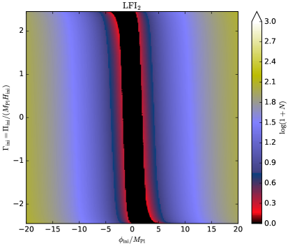
Figure 1: Number of e-folds of inflation for $\mathrm{LFI}_{2}$ achieved along phase-space trajectories starting from $2048^{2}$ initial conditions. No fine-tuning is required as almost all initial conditions lead to inflation, independently of the initial kinetic energy stored in the inflaton. At fixed value of $\Phi_{\mathrm{ini}}>0$, we notice that the number of e-folds is less if $\Gamma_{\mathrm{ini}}<0$ than it is for $\Gamma_{\mathrm{ini}}>0$. This effect is especially clear when $\Gamma_{\mathrm{ini}}$ is close to its extremal value $\pm\sqrt{6}$ and $\Phi_{\mathrm{ini}}$ is not too large. This is because, if $\Gamma_{\mathrm{ini}}<0$, then the field is initially pushed toward the minimum of the potential, while if $\Gamma_{\mathrm{ini}}>0$, it initially climbs up the potential (the situation is symmetric for $\Phi_{\mathrm{ini}}<0$).

Let us first examine the case of large-field inflation ($\mathrm{LFI}{}_{p}$) with potential $V(\phi)=M^{4}(\phi/M_{\scriptscriptstyle{\mathrm{Pl}}})^{p}$, where $p>0$. The slow-roll solution for positive field values can be easily derived and reads Martin et al. (2014a)

$$\Phi(N)=\sqrt{\dfrac{p^{2}}{2}-2p\left(N-N_{\mathrm{end}}\right)}\,.$$ (49)

The transitional phase described by Eq. (19) reaches this solution after a field excursion $\Delta\Phi$. As discussed in Sec. II.1.5, in all regions where $|\Gamma_{\mathrm{sr}}|\ll 1$, one has

$$\Delta\Phi\simeq\Delta\Phi_{\times}\simeq\Delta\Phi_{\max},$$ (50)

where $\Delta\Phi_{\max}$ is given in Eq. (24). Here, as described before, we use $\Gamma_{\times}=\pm|\Gamma_{\mathrm{sr}}|$. From the above trajectory (49), a total number $\mathcal{N}_{\mathrm{inf}}$ of e-folds is realized in the slow-roll regime if the field reaches the attractor at a vacuum expectation value given by $M_{\scriptscriptstyle{\mathrm{Pl}}}\sqrt{p^{2}/2+2p\mathcal{N}_{\mathrm{inf}}}$. As a consequence, requiring slow-roll inflation to last more than $\mathcal{N}_{\mathrm{inf}}$ e-folds means $\Phi_{\times}>\sqrt{p^{2}/2+2p\mathcal{N}_{\mathrm{inf}}}$, or

$$\Phi_{\mathrm{ini}}+\dfrac{1}{\sqrt{6}}\ln\left(\dfrac{1+\dfrac{\Gamma_{\mathrm{ini}}}{\sqrt{6}}}{1-\dfrac{\Gamma_{\mathrm{ini}}}{\sqrt{6}}}\right)>\sqrt{\dfrac{p^{2}}{2}+2p\mathcal{N}_{\mathrm{inf}}}\simeq 2\sqrt{30p}\,,$$ (51)

where the last equality comes from choosing $\mathcal{N}_{\mathrm{inf}}=60$ e-folds. For even values of $p$, the potential is symmetric with respect to $\Phi=0$ and negative initial field values verify the opposite of the above bound. From Eq. (51), we see that no fine-tuning of the initial field values is required to start inflation. On the contrary, only an extreme fine-tuning of $\Gamma_{\mathrm{ini}}$ close to $-\sqrt{6}$ might demand to push $\Phi_{\mathrm{ini}}$ to larger positive values to start inflation.

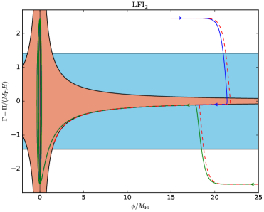
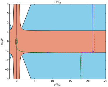
Figure 2: Phase-space trajectories for $\mathrm{LFI}_{2}$ (solid curves) starting deeply in the kination regime and relaxing toward slow roll. The blue line corresponds to a situation where the field initially climbs up its potential while the green line represents a case where it rolls it down. The upper panel displays the phase space $(\Phi,\Gamma)$ while the lower panel corresponds to $(\phi,\Pi)$. The analytical approximations of Eqs. (10) and (19) are represented as dashed red curves. In the upper figure, the horizontal blue region corresponds to $\Gamma^{2}<2$, i.e., inflation. The orange region narrowing at large-field values is the domain for which $|\Gamma|\leq|\Gamma_{\mathrm{sr}}|$. Both regions are also represented in the lower panel.

This is confirmed in Fig. 1, which shows the number of e-folds of inflation achieved for $p=2$, starting from a grid of $2048^{2}$ initial conditions. Almost the whole phase-space produces inflation, without any fine-tuning of the initial conditions. The inverted “S” shape of the contours of equal e-foldings is well described by Eq. (51). This may appear surprising as, strictly speaking, Eq. (51) is valid only for $|\Gamma|\gg|\Gamma_{\mathrm{sr}}|$. However, as explained in Sec. II.1.5, for small values of $|\Gamma_{\mathrm{sr}}|$, this inequality can only be violated (namely $\Gamma<\Gamma_{\mathrm{sr}}$) at small values of $|\Gamma|$. Since $\Gamma\propto\mathrm{d}\Phi/\mathrm{d}N$, this happens only in regions where the field value is nearly constant, and Eq. (51) is essentially valid almost everywhere in phase-space.

In order to compare the analytical approximations presented in Sec. II.1.2 to the exact results, a few trajectories have been represented in Fig. 2. The upper panel shows trajectories in the phase-space $(\Phi,\Gamma)$ while the lower panel is for $(\phi,\Pi)$. The blue region encompasses values of $\Gamma^{2}<2$ corresponding to an accelerated expansion of the universe. The orange region (contained within the blue one at large-field values) represents values of $|\Gamma|\leq|\Gamma_{\mathrm{sr}}|$. The solid curves are two numerical integrated trajectories starting deeply in the kination regime, i.e., with $\Gamma^{2}$ fine-tuned to $6$. They rapidly relax toward the boundary between the blue and the orange regions where they match the slow-roll attractor $\Gamma=\Gamma_{\mathrm{sr}}$.

The dashed red curves represent the simplified analytical solution discussed in Sec. II.1.5, made of Eq. (19) extrapolated till it crosses $\Gamma_{\times}=\pm|\Gamma_{\mathrm{sr}}|$ and, eventually, extrapolated again to $\Gamma_{\mathrm{sr}}$ at constant $\Phi$. In other words, we have neglected both $\mathcal{C}(N)$ and the relaxation terms in Eq. (31). Even with such a crude extrapolation, we find good agreement with the exact numerical result almost everywhere. For the purpose of illustration, we have extended by a fraction of e-folds the exact trajectories in the regime $H<H_{\mathrm{end}}$ in order to show a few oscillations around the minimum of the potential. Let us notice that, in the oscillatory domain, $\Gamma_{\mathrm{sr}}(\Phi)$ blows up and none of the analytical approximations presented before can be used. A more detailed investigation of these regions is presented in Sec. II.4.

We conclude, as is well known, that no fine-tuning of initial conditions is necessary for large-field inflation.

II.2.3 Small-field inflation

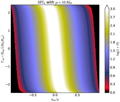
Figure 3: Number of e-folds of inflation for $\mathrm{SFI}_{4}$ achieved along phase-space trajectories starting from $2048^{2}$ initial conditions. Some fine-tuning is required for $\mu<M_{\scriptscriptstyle{\mathrm{Pl}}}$ (upper panel) while almost all initial conditions lead to inflation for $\mu>M_{\scriptscriptstyle{\mathrm{Pl}}}$ (lower panel). We see (upper panel) that if the field is not initially extremely close to the origin and starts at, say, positive values, then the only way to obtain a large number of e-folds of inflation is to tune its velocity such that it initially climbs up the potential (namely $\Gamma_{\mathrm{ini}}<0$) and reaches the maximum with almost vanishing velocity.

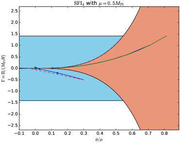
Figure 4: Phase-space trajectories for $\mathrm{SFI}_{4}$ (solid curve) in the fine-tuning regime for $\mu<M_{\scriptscriptstyle{\mathrm{Pl}}}$, in the space ($\Phi,\Gamma$). The lower panel is a zoom in the region around $\phi=0$. The analytical approximations are represented with dashed-red curves and match well the exact result displayed with the green curve. The agreement with the blue curve is less compelling since the initial value of $|\Gamma/\Gamma_{\mathrm{sr}}|$ is not so large in that case. The analytical formula thus hits slow roll (the boundary of the orange region) on the wrong side of the potential, i.e., at $\phi<0$ instead of $\phi>0$, and hence cannot be used subsequently. Notice that in both cases, the inflationary exit is not well described by slow roll, precisely due to the steepness of the potential for $\phi$ approaching $\mu$. Because $V(\phi)\simeq M^{4}$ in the limit $\mu\ll M_{\scriptscriptstyle{\mathrm{Pl}}}$, trajectories in the space $(\phi,\Pi)$ are almost identical and have not been represented (see also Fig. 5).

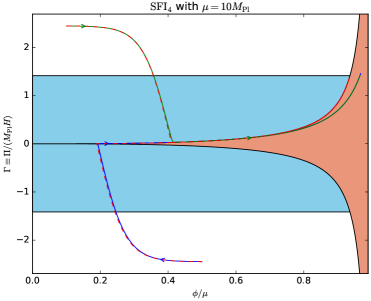
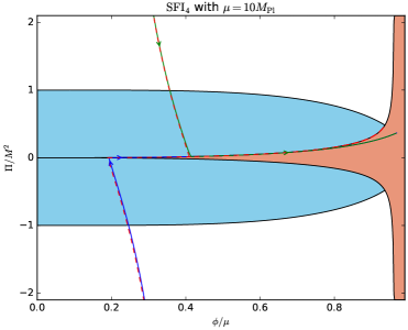
Figure 5: Phase-space trajectories for $\mathrm{SFI}_{4}$ (solid curve) with $\mu>M_{\scriptscriptstyle{\mathrm{Pl}}}$. As for the large-field models, almost all initial conditions relax toward slow roll and no fine-tuning is needed to start inflation. The upper panel displays the phase-space $(\Phi,\Gamma)$ while the lower panel corresponds to $(\phi,\Pi)$. Our analytical approximations have been plotted in dashed red. The blue region corresponds to $\Gamma^{2}<2$, i.e., inflation, while the orange region widening toward $\phi/\mu=1$ is the domain for which $|\Gamma|\leq|\Gamma_{\mathrm{sr}}|$.

We now consider the case of the small-field inflation models $\mathrm{SFI}_{p}$, with potential

$$V(\phi)=M^{4}\left[1-\left(\frac{\phi}{\mu}\right)^{p}\right],$$ (52)

where $\mu$ is a mass scale and $p\geq 2$ a power index. This potential has no minimum and becomes negative if $\phi>\mu$. For this reason $V(\phi)$ can be trusted only if $\phi<\mu$.

The slow-roll solution for $\mathrm{SFI}$ can be found in Ref. Martin et al. (2014a) and reads

$$2p\dfrac{M_{\scriptscriptstyle{\mathrm{Pl}}}^{2}}{\mu^{2}}\left(N_{\mathrm{end}}-N\right) =\dfrac{2}{p-2}\left(x^{2-p}-x_{\mathrm{end}}^{2-p}\right)+x^{2}-x_{\mathrm{end}}^{2},$$ (53)

where we have defined

$$x(N)\equiv\dfrac{\phi(N)}{\mu}=\dfrac{M_{\scriptscriptstyle{\mathrm{Pl}}}}{\mu}\Phi(N),$$ (54)

and $x_{\mathrm{end}}$ is the slow-roll solution $\Gamma_{\mathrm{sr}}^{2}(x_{\mathrm{end}})=2$ for the end of inflation,

$$x_{\mathrm{end}}^{p}+\dfrac{p}{\sqrt{2}}\dfrac{M_{\scriptscriptstyle{\mathrm{Pl}}}}{\mu}x_{\mathrm{end}}^{p-1}=1.$$ (55)

The above equations are also valid in the limit $p\to 2$ and can be used to study $\mathrm{SFI}_{2}$. Let us, however, stress that consistency of slow roll within $\mathrm{SFI}_{2}$ imposes the additional constraint $\mu>M_{\scriptscriptstyle{\mathrm{Pl}}}$, see Ref. Martin et al. (2014a).

As above, using Eq. (24) to approximate the transitional regime before reaching slow roll, one has

$$x_{\times}\simeq x_{\mathrm{ini}}+\dfrac{1}{\sqrt{6}}\dfrac{M_{\scriptscriptstyle{\mathrm{Pl}}}}{\mu}\ln\left(\dfrac{1+\dfrac{\Gamma_{\mathrm{ini}}}{\sqrt{6}}}{1-\dfrac{\Gamma_{\mathrm{ini}}}{\sqrt{6}}}\right).$$ (56)

Slow roll produces $N_{\mathrm{end}}-N_{\times}>\mathcal{N}_{\mathrm{inf}}$ e-folds of inflation provided $x_{\times}$ satisfies

$$\dfrac{2}{p-2}x_{\times}^{2-p}+x_{\times}^{2}>2p\dfrac{M_{\scriptscriptstyle{\mathrm{Pl}}}^{2}}{\mu^{2}}\mathcal{N}_{\mathrm{inf}}+\dfrac{2}{p-2}x_{\mathrm{end}}^{2-p}+x_{\mathrm{end}}^{2}.$$ (57)

Plugging Eq. (56) into Eq. (57) gives the necessary condition for a trajectory starting at $(x_{\mathrm{ini}},\Gamma_{\mathrm{ini}})$ to produce $\mathcal{N}_{\mathrm{inf}}$ e-folds of slow-roll inflation. As it is obvious from these expressions, the amount of fine-tuning strongly depends on the ratio $\mu/M_{\scriptscriptstyle{\mathrm{Pl}}}$.

Let us first assume that $\mu\ll M_{\scriptscriptstyle{\mathrm{Pl}}}$. As can be seen in Eq. (56), this regime amplifies the effect of $\Gamma_{\mathrm{ini}}$ in the actual value of $x_{\times}$ at fixed $x_{\mathrm{ini}}$. Moreover, from Eq. (55), one has

$$x_{\mathrm{end}}\simeq\left(\dfrac{\sqrt{2}}{p}\dfrac{\mu}{M_{\scriptscriptstyle{\mathrm{Pl}}}}\right)^{1/(p-1)}\ll 1,$$ (58)

and the whole slow-roll region $x\leq x_{\mathrm{end}}$ is confined in a small domain at the top of the potential. The terms in $x_{\times}^{2}$ and $x_{\mathrm{end}}^{2}$ in Eq. (57) can be neglected in this limit (recall that $p>2$). One finally gets, for $p>2$,

$$x_{\mathrm{ini}} +\dfrac{1}{\sqrt{6}}\dfrac{M_{\scriptscriptstyle{\mathrm{Pl}}}}{\mu}\ln\left(\dfrac{1+\dfrac{\Gamma_{\mathrm{ini}}}{\sqrt{6}}}{1-\dfrac{\Gamma_{\mathrm{ini}}}{\sqrt{6}}}\right)$$ (59)

$$<\left[p(p-2)\dfrac{M_{\scriptscriptstyle{\mathrm{Pl}}}^{2}}{\mu^{2}}\mathcal{N}_{\mathrm{inf}}+\left(\dfrac{p}{\sqrt{2}}\dfrac{M_{\scriptscriptstyle{\mathrm{Pl}}}}{\mu}\right)^{\frac{p-2}{p-1}}\right]^{-\frac{1}{p-2}}.$$

The right-hand side of this expression is a very small number for $\mu\ll M_{\scriptscriptstyle{\mathrm{Pl}}}$, showing that $x_{\mathrm{ini}}$ and $\Gamma_{\mathrm{ini}}$ should be fine-tuned along a narrow band in phase-space to produce a successful inflationary era. Let us stress, however, that such a fine-tuning is not only related to the presence of an initial kinetic energy. Setting $\Gamma_{\mathrm{ini}}=0$ in the previous equations does not solve the issue as $x_{\mathrm{ini}}$ still has to be tuned at the top of the potential. The fine tuning comes from the small field extension of the domain allowing for long-enough inflation when $\mu\ll M_{\scriptscriptstyle{\mathrm{Pl}}}$.

Taking the opposite limit, namely $\mu\gg M_{\scriptscriptstyle{\mathrm{Pl}}}$, one gets

$$x_{\mathrm{end}}\simeq 1-\dfrac{M_{\scriptscriptstyle{\mathrm{Pl}}}}{\sqrt{2}\mu},$$ (60)

while, at leading order in $M_{\scriptscriptstyle{\mathrm{Pl}}}/\mu$, Eq. (57) becomes

$$x_{\times}<1-\dfrac{M_{\scriptscriptstyle{\mathrm{Pl}}}}{\mu}\sqrt{\dfrac{1}{2}+2\mathcal{N}_{\mathrm{inf}}}\,.$$ (61)

Long enough inflation is therefore triggered for any initial conditions satisfying

$$x_{\mathrm{ini}} +\dfrac{1}{\sqrt{6}}\dfrac{M_{\scriptscriptstyle{\mathrm{Pl}}}}{\mu}\ln\left(\dfrac{1+\dfrac{\Gamma_{\mathrm{ini}}}{\sqrt{6}}}{1-\dfrac{\Gamma_{\mathrm{ini}}}{\sqrt{6}}}\right)<1-\dfrac{M_{\scriptscriptstyle{\mathrm{Pl}}}}{\mu}\sqrt{\dfrac{1}{2}+2\mathcal{N}_{\mathrm{inf}}}\,,$$ (62)

and there is no fine-tuning for $\mu\gg M_{\scriptscriptstyle{\mathrm{Pl}}}$.

These findings are confirmed by the numerical results of Fig. 3 where the case of $\mathrm{SFI}_{4}$ is presented. For $\mu=0.5M_{\scriptscriptstyle{\mathrm{Pl}}}$ (top panel), one recovers the thin, fine-tuned band as predicted by Eq. (59), but its shape is distorted for $\phi_{\mathrm{ini}}/\mu\gtrsim 0.1$. This is expected because $\Gamma_{\mathrm{sr}}(\Phi)$ is no longer a small quantity in these regions and the hypothesis $|\Gamma|\gg|\Gamma_{\mathrm{sr}}|$ ceases to be accurate. For $\mu=10M_{\scriptscriptstyle{\mathrm{Pl}}}$ (bottom panel), the contours of equal e-foldings are in perfect agreement with the functional shape of Eq. (62) and no fine-tuning is necessary to trigger inflation. The situation is at all points similar to the large-field models discussed in Sec. II.2.2. Phase-space trajectories for $\mathrm{SFI}_{4}$ are represented in Figs. 4 and 5.

II.2.4 Initial conditions problem in hilltop models

The small-field models discussed in the previous section are also referred to as “hilltop models” in the literature Boubekeur and Lyth (2005); Tzirakis and Kinney (2007); Enckell et al. (2018) and the previous results allow us to discuss various claims made in Ref. Ijjas et al. (2013) about them.

Reference Ijjas et al. (2013) argues that, on general grounds, the Planck data disfavors the large-field $\mathrm{LFI}_{p}$ models compared to $\mathrm{SFI}_{p}$, postulated to be all fine-tuned. In other words, Planck would have shown that inflation is in trouble since the data favor a class of models for which the choice of initial conditions is unnatural. However, we have just seen that this is not the case. All $\mathrm{SFI}_{p}$ models with $\mu\gg M_{\scriptscriptstyle{\mathrm{Pl}}}$ are free of fine-tuning issues, at least in the very same manner as the $\mathrm{LFI}_{p}$ models are. Moreover, as can be checked in Ref. Martin et al. (2014b), although the Planck data indeed make the Bayesian evidence of $\mathrm{LFI}$ smaller than the one of $\mathrm{SFI}$, within the $\mathrm{SFI}$ models, they slightly disfavor the $\mathrm{SFI}$ scenarios having $\mu<M_{\scriptscriptstyle{\mathrm{Pl}}}$ compared to the ones with $\mu>M_{\scriptscriptstyle{\mathrm{Pl}}}$. Let us stress that the CMB data are blind to the initial conditions of inflation and this result only comes from the observable values of the tensor-to-scalar ratio and the spectral index. It means that, even for $p\neq 2$, the models $\mathrm{SFI}_{p>2}$ favored after Planck actually have fewer problems with regards to the initial conditions than the models favored before Planck.

Even if the previous argument is clearly in favor of inflation, it is, in fact, anecdotal since the $\mathrm{SFI}$ models are not belonging to the most favored models. In terms of Bayesian evidence, the most probable models are the plateau models Martin et al. (2014b). These plateau models are very different (in particular, with respect to the initial conditions problem) from hilltop/$\mathrm{SFI}$ models and should not be confused. The terminology of Ref. Ijjas et al. (2013), which includes them in the same category, is therefore problematic from that perspective. The typical example of plateau inflation is the Starobinsky model that we discuss in the next section.

II.3 Plateau is not hilltop!

Figure 6: Number of e-folds of inflation for $\mathrm{SI}$ achieved along phase-space trajectories starting from $2048^{2}$ initial conditions. Plateau-like models are very different from hilltop models. Almost all positive field values lead to slow-roll inflation, even for large kinetic energies.

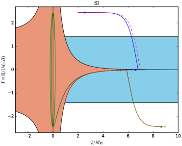
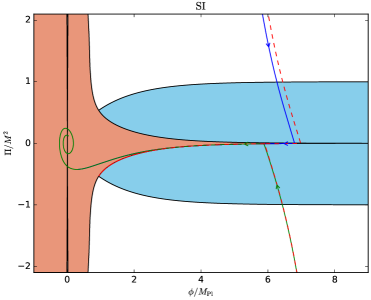
Figure 7: Phase-space trajectories for $\mathrm{SI}$ (solid curve) starting deeply in the kination regime and relaxing toward slow roll. The upper panel corresponds to the phase-space $(\Phi,\Gamma)$ while the lower panel is for $(\phi,\Pi)$. Our analytical approximations are represented as dashed red curves. The slight shift between the analytical and the exact upper trajectories comes from the fact that $\Gamma_{\mathrm{sr}}$ (the boundary of the orange region) is not small compared to $\Gamma_{\mathrm{ini}}$. The steepness of the potential toward its minimum slightly affects the kination regime described by Eq. (19). Such an effect rapidly disappears at larger field values, as can be seen for the lower trajectory.

In this section, we consider the Starobinsky model ($\mathrm{SI}$) which exemplifies plateau inflation. As we will see, contrary to small-field inflation, no fine-tuning is required to start inflation. The potential is given by Martin et al. (2014a)

$$V(\phi)=M^{4}\left[1-\exp\left(-\sqrt{\frac{2}{3}}\frac{\phi}{M_{\scriptscriptstyle{\mathrm{Pl}}}}\right)\right]^{2},$$ (63)

and the slow-roll solution reads

$$e^{\sqrt{\frac{2}{3}}\Phi(N)}-\sqrt{\dfrac{2}{3}}\Phi(N) =\dfrac{4}{3}\left(N_{\mathrm{end}}-N\right)$$ (64)

$$+1+\dfrac{2}{\sqrt{3}}-\ln\left(1+\dfrac{2}{\sqrt{3}}\right).$$

As before, matching the kinetically driven regime to slow roll at $\Phi_{\times}$ gives the condition for $(\Phi_{\mathrm{ini}},\Gamma_{\mathrm{ini}})$ to produce $N_{\mathrm{end}}-N_{\times}>\mathcal{N}_{\mathrm{inf}}$ e-folds of slow-roll inflation. One gets

$$e^{\sqrt{\frac{2}{3}}\Phi_{\mathrm{ini}}}\left(\dfrac{1+\dfrac{\Gamma_{\mathrm{ini}}}{\sqrt{6}}}{1-\dfrac{\Gamma_{\mathrm{ini}}}{\sqrt{6}}}\right)^{\frac{1}{3}}-\sqrt{\dfrac{2}{3}}\Phi_{\mathrm{ini}}-\dfrac{1}{3}\ln\left(\dfrac{1+\dfrac{\Gamma_{\mathrm{ini}}}{\sqrt{6}}}{1-\dfrac{\Gamma_{\mathrm{ini}}}{\sqrt{6}}}\right)$$ (65)

$$>\dfrac{4}{3}\mathcal{N}_{\mathrm{inf}}+1+\dfrac{2}{\sqrt{3}}-\ln\left(1+\dfrac{2}{\sqrt{3}}\right).$$

No fine-tuning is necessary to satisfy such a condition. Compared to $\mathrm{LFI}$, see Eq. (51), the presence of the exponential ensures that slow-roll inflation always occurs even for relatively low values of $\Phi_{\mathrm{ini}}$. The numerical integration of the number of e-folds is shown in Fig. 6 and matches well Eq. (65). The relaxation toward slow roll of a few trajectories starting deeply in the kination regime is represented in Fig. 7.

The results of this section are probably the most important ones regarding the initial conditions problem. In short, Planck favors models, namely single-field plateau potentials, for which there is no initial conditions problem at all. This is why inflation is not “in trouble” after Planck but, on the contrary, is rather reinforced.

II.4 The “unlikeliness problem of inflation”

Reference Ijjas et al. (2013) also argues that inflation is “exponentially unlikely according to the inner logics of the inflationary paradigm itself” and that this problem is an additional issue for inflation, independent of the initial conditions problem previously discussed. The potential chosen by the authors to exemplify this issue is $V(\phi)\propto[1-(\phi/\phi_{{}_{0}})^{2}]^{2}$ [the potential was written $V(\phi)=\lambda(\phi^{2}-\phi_{0}^{2})^{2}$; see Fig. 1(a) of that paper], which possesses a hilltop domain, at $\phi<\phi_{0}$, and a large-field one, at $\phi>\phi_{0}$. The “unlikeliness problem” is the claim that inflation is more likely to occur in the latter, whereas the data prefer the former.

The model is again referred to as a “plateau-like model”. The leading-order expansion of the potential in $\phi\ll\phi_{{}_{0}}$ is Eq. (52) with $p=2$, $M^{4}=\lambda\phi_{0}^{4}$ and $\mu=\phi_{0}/\sqrt{2}$. Equation (3) of Ref. Ijjas et al. (2013) suggests that only the regime $\mu<M_{\scriptscriptstyle{\mathrm{Pl}}}$ is considered, while it is stated that $\phi\ll\phi_{{}_{0}}$ is required for inflation to occur. Their terminology “plateau-like” is therefore unambiguously referring to $\mathrm{SFI}_{2}$ models with sub-Planckian vev (which we have shown in Sec. II.2.3 suffer from an initial-conditions fine-tuning issue).

As we have argued before, this terminology is inappropriate as “plateau” is not “hilltop”. More importantly, the choice $p=2$ is a very particular case. Because it is a hilltop model with a non-vanishing mass, as discussed at length in Ref. Martin et al. (2014a), $\mathrm{SFI}_{2}$ with $\mu<2M_{\scriptscriptstyle{\mathrm{Pl}}}$ does not support slow-roll inflation at all, the spectral index is very far from scale invariance and this model is ruled out by any CMB data. Within all possible $\mathrm{SFI}_{2}$ models, only the ones having super-Planckian $\mu>2M_{\scriptscriptstyle{\mathrm{Pl}}}$ can be made compatible with CMB measurements, and from Eq. (62), super-Planckian $\mathrm{SFI}_{2}$ models do not suffer from any fine-tuning issues.

In order to study the “unlikeliness problem”, Ref. Ijjas et al. (2013) needs, in fact, a model with a small-field part and a large-field part, the latter being interpreted as a reasonable UV completion of the former. Although the choice of $V(\phi)\propto[1-(\phi/\phi_{{}_{0}})^{2}]^{2}$ is quite unfortunate, consistent slow-roll models having this property exist and, in the following, we study two explicit examples. It is worth noticing again that these types of models are not plateau-like and, therefore, are not among the best models according to the Planck data. This implies, as discussed at the end of Sec. II.2.4, that the “unlikeliness problem”, if it exists, can only affect models that are not favored by the data. Nevertheless, let us be exhaustive in our discussion of the criticisms raised against inflation.

II.4.1 Generalized double-well inflation

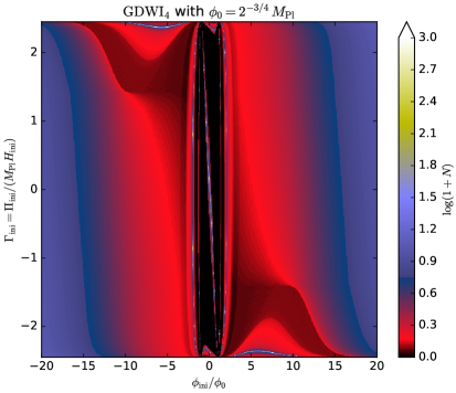
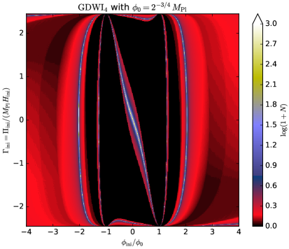
Figure 8: Number of e-folds of inflation for the fine-tuned $\mathrm{GDWI}_{4}$ model ($\phi_{{}_{0}}<M_{\scriptscriptstyle{\mathrm{Pl}}}$) achieved along phase-space trajectories starting from $2048^{2}$ initial conditions. The lower panel is a zoom into the central region for which $-4\phi_{{}_{0}}<\phi<4\phi_{{}_{0}}$. The light narrow band in the middle is identical to the one obtained for $\mathrm{SFI}_{4}$ in Fig. 3. However, the completed potential of $\mathrm{GDWI}_{4}$ now allows for new successful initial conditions. The narrow band expands and spirals into steep regions of the potential.

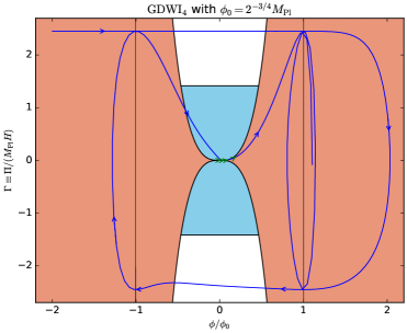
Figure 9: A phase-space trajectory for the fine-tuned $\mathrm{GDWI}_{4}$ model ($\phi_{{}_{0}}<M_{\scriptscriptstyle{\mathrm{Pl}}}$), starting in kination and in a region of the potential that is steep, $\Gamma_{\mathrm{sr}}(\Phi_{\mathrm{ini}})>\Gamma_{\mathrm{ini}}\simeq\sqrt{6}$. Compared to $\mathrm{SFI}_{4}$, the UV-completed potential allows for a complex bouncing dynamics that makes this trajectory producing hundreds of e-folds of hilltop inflation (around the green horizontal arrows at $\phi\simeq 0$). These trajectories are responsible for the multiplication of the successful inflationary regions in Fig. 8.

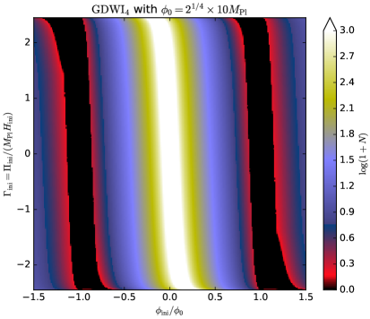
Figure 10: Number of e-folds of inflation for the $\mathrm{GDWI}_{4}$ model in the non-fine-tuned regime ($\phi_{{}_{0}}>M_{\scriptscriptstyle{\mathrm{Pl}}}$) along $2048^{2}$ phase-space trajectories. The large inflationary band in the middle is identical to the one obtained for $\mathrm{SFI}_{4}$ in Fig. 3. The structure of the successful domain is not affected by the UV completion.

In this section, we consider the generalized double-well model ($\mathrm{GDWI}_{2p}$), the potential of which can be written as

$$V(\phi)=M^{4}\left[\left(\frac{\phi}{\phi_{{}_{0}}}\right)^{2p}-1\right]^{2},$$ (66)

where $\phi_{{}_{0}}$ is a vev and $p$ a positive power index. For $\phi\ll\phi_{{}_{0}}$, Eq. (66) can be expanded as

$$V(\phi)\simeq M^{4}\left[1-2\left(\dfrac{\phi}{\phi_{{}_{0}}}\right)^{2p}\right].$$ (67)

The case $p=1$ corresponds to the so-called double-well inflation ($\mathrm{DWI}$) studied in Sec. 4.14 of Ref. Martin et al. (2014a). As discussed in this reference, $\mathrm{DWI}$ can be viewed as a UV completion of $\mathrm{SFI}_{2}$ with $\mu=\phi_{{}_{0}}/\sqrt{2}$. However, it is shown in this reference that slow-roll inflation can only occur for $\phi_{{}_{0}}>2\sqrt{2}M_{\scriptscriptstyle{\mathrm{Pl}}}$, for which there is no fine-tuning of the initial conditions. This potential is therefore of limited interest to discuss how the fine-tuning could be affected by the large-field completion of the potential. As discussed previously, $\mathrm{DWI}$ is the potential chosen in Ref. Ijjas et al. (2013) to supposedly illustrate the fine-tuning of hilltop inflation.

The power index $p=2$ is, however, of immediate interest. As can be seen from Eq. (67), $\mathrm{GDWI}_{4}$ provides a large-field completion of $\mathrm{SFI}_{4}$ with $\mu=2^{-1/4}\phi_{{}_{0}}$. For $\phi\gg\phi_{{}_{0}}$, Eq. (66) behaves as the large-field model $\mathrm{LFI}_{4p}$. The initial conditions to start inflation are given by Eq. (51) and are not fine-tuned. In the small-field regime, they are given by Eqs. (59) and (62) and are either fine-tuned for $\phi_{{}_{0}}<M_{\scriptscriptstyle{\mathrm{Pl}}}$, or not fine-tuned for $\phi_{{}_{0}}>M_{\scriptscriptstyle{\mathrm{Pl}}}$.

In Fig. 8, we have represented the number of inflationary e-folds as a function of initial conditions for $p=2$ and $\phi_{{}_{0}}=2^{-3/4}M_{\scriptscriptstyle{\mathrm{Pl}}}$. This corresponds to the fine-tuning regime of $\mathrm{SFI}_{4}$ with $\mu=0.5M_{\scriptscriptstyle{\mathrm{Pl}}}$. In the central region, for $\phi\simeq 0$, we recover exactly the same structure as in $\mathrm{SFI}_{4}$. The shape and position of the narrow band in which inflation occurs are the same (see Fig. 3). However, for $\phi/\phi_{{}_{0}}\gtrsim 1$, new successful inflationary regions appear. They are extensions of the central narrow band that are spiraling many times into the steep parts of the UV-completed potential. Their origin is evident from the example trajectory plotted in Fig. 9. Starting with a large kinetic energy in a steep region of the potential, the field may cross the local maximum at $\phi=0$ one or several times before falling into one of the two minima. For some values of the initial kinetic energy, the last crossing occurs with small enough velocity to enter a phase of slow-roll inflation. This does not solve the fine-tuning problem of $\mathrm{SFI}_{4}$ with $\mu<M_{\scriptscriptstyle{\mathrm{Pl}}}$, since the regions of successful initial conditions in phase-space remain of small size. Still, the presence of a large-field branch in the potential increases the size of the successful regions of inflation rather than diminishing them.

In Fig. 10, we have represented the number of inflationary e-foldings in phase-space for $\mathrm{GDWI}_{4}$ in the regime without fine-tuning, for $\phi/\phi_{{}_{0}}=2^{1/4}\times 5M_{\scriptscriptstyle{\mathrm{Pl}}}$. The central region matches the one of $\mathrm{SFI}_{4}$ with $\mu=10M_{\scriptscriptstyle{\mathrm{Pl}}}$ (see Fig. 3) and there is no fine-tuning. Interestingly, there are no longer trajectories spiraling around the central region. This is due to the fact that the potential is flat enough, namely $|\Gamma_{\mathrm{sr}}|\ll 1$, all over the region $\phi/\phi_{{}_{0}}\lesssim 1$. Therefore, even if $|\Gamma_{\mathrm{ini}}|$ is large, Eq. (62) applies: the system relaxes toward slow roll and cannot cross the whole hilltop region.

Let us now discuss the “unlikeliness problem” in the light of these results. In a double-well potential with super-Planckian well separation ($\phi_{0}>M_{\scriptscriptstyle{\mathrm{Pl}}}$), the data strongly support the hilltop region of the potential against the large-field one, but there is no fine-tuning issue of the initial conditions in either region, hence there is no unlikeliness problem. If the well separation is sub-Planckian ($\phi_{0}<M_{\scriptscriptstyle{\mathrm{Pl}}}$) and the effective mass does not vanish at the top of the hill ($p=1$ or $\mathrm{GDWI}_{2}$), both inflating regions of the potential are strongly disfavored by the data and the entire potential is excluded. There is therefore no unlikeliness problem in that case either. Only if the well separation is sub-Planckian and the hill mass vanishes, the favored region of the potential, i.e., the hilltop one, suffers from initial-conditions fine-tuning, though this fine-tuning is not reinforced by the UV completion (it is rather the contrary as discussed before). It is the only situation where one could argue in favor of an “unlikeliness problem”. This, however corresponds to a very specific choice of the inflationary potential, that is anyway disfavored compared to plateau models Martin et al. (2014b).

II.4.2 Coleman-Weinberg inflation

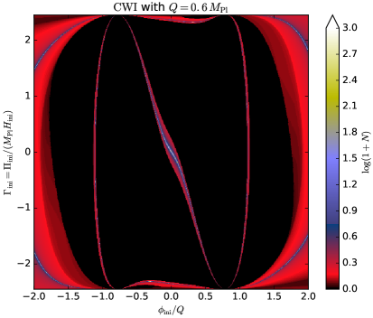
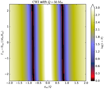
Figure 11: Number of e-folds of inflation in the $\mathrm{CWI}$ model for $2048^{2}$ initial conditions. The upper panel is in the fine-tuning regime $Q<M_{\scriptscriptstyle{\mathrm{Pl}}}$ while the bottom panel if for $Q>M_{\scriptscriptstyle{\mathrm{Pl}}}$. The situation is generic of hilltop inflation, see also Figs. 8 and 10.

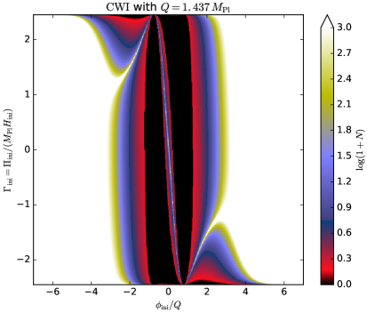
Figure 12: Number of e-folds of inflation in the $\mathrm{CWI}$ double inflationary regime, for $Q\simeq 1.4\,M_{\scriptscriptstyle{\mathrm{Pl}}}$. All initial conditions in the large-field regime, $\phi_{\mathrm{ini}}/Q>1$, produce trajectories climbing up into the central hilltop narrow band. There is no fine-tuning of the initial conditions anymore, and the observable window (i.e., the last $\sim 60$ e-folds of inflation) is always in the hilltop domain of the potential, even though this regime would appear fine-tuned without the UV completion of the potential.

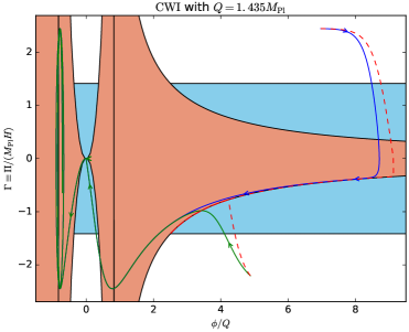
Figure 13: Example trajectories for $\mathrm{CWI}$ in the double inflation regime, for $Q=1.435\,M_{\scriptscriptstyle{\mathrm{Pl}}}$. The two trajectories represented as solid lines start in the large-field inflationary region and end up producing about $500$ e-folds of hilltop inflation around $\phi\simeq 0$. The dashed red curves are the analytical approximations in the large-field regime and can be used only in that region.

Figure 14: Number of e-folds of hilltop inflation realized within the $\mathrm{CWI}$ double-inflation regime. Because of the slow-roll attractor in the large-field domain, it depends only on the scale $Q$.

Although discussed for $\mathrm{GDWI}_{4}$ only, we expect the previous findings to be a generic property of the hilltop models. In this section, we indeed recover them in a particle-physics motivated model: the Coleman-Weinberg potential (CWI) Linde (1982)

$$V(\phi)=M^{4}\left[1+2e\left(\dfrac{\phi}{Q}\right)^{4}\ln\left(\dfrac{\phi^{2}}{Q^{2}}\right)\right].$$ (68)

The potential vanishes at its two minima for $\phi/Q=\pm e^{-1/4}$ and supports both hilltop inflation for $|\phi/Q|<e^{-1/4}$ and large-field-like inflation for $|\phi/Q|>e^{-1/4}$. Slow-roll solutions have been derived in Ref. Martin et al. (2014a) and can be used together with Eq. (24) to derive the initial conditions required to get enough e-folds of inflation in the hilltop region. The situation is very similar to Sec. II.2.3 and we do not reproduce the calculations here. The region $|\Gamma_{\mathrm{sr}}|\ll 1$ is very confined around $\phi=0$ when $Q<M_{\scriptscriptstyle{\mathrm{Pl}}}$ and starting inflation is fine-tuned in that case.

The full numerical integration of $\mathrm{CWI}$ in the fine-tuning regime, with $Q=0.6M_{\scriptscriptstyle{\mathrm{Pl}}}$, is presented in the upper panel of Fig. 11. The situation is in all points similar to $\mathrm{GDWI}_{4}$ (see Fig. 8). The narrow region of successful initial conditions is extended into a spiraling band exploring the steep parts of the potential that slightly alleviates the fine-tuning problem. For completeness, we have also represented in the bottom panel of Fig. 11 the non-fine-tuned case $Q=50\,M_{\scriptscriptstyle{\mathrm{Pl}}}$, where the whole hilltop region $\phi_{\mathrm{ini}}/Q<1$ inflates.

A very interesting phenomenon appears for Planckian-like expectation values $Q=\mathcal{O}\!\left(M_{\scriptscriptstyle{\mathrm{Pl}}}\right)$, the large-field region becomes connected to the hilltop one. The kinetic energy acquired by the field when exiting the large-field inflationary regime may become large enough to climb into the hilltop domain, thereby triggering a second inflationary era (see Fig. 12). Such an effect is not generic of hilltop models as it clearly depends on how the hilltop domain is UV completed. For the Coleman-Weinberg potential, we find that double inflation appears for $Q\simeq 1.4\,M_{\scriptscriptstyle{\mathrm{Pl}}}$ Yokoyama (1998). For such a value of $Q$, even though the hilltop regime is still rather fine-tuned, all large-field trajectories end up in the narrow inflationary band at the top of the potential. As a result, the fine tuning of $(\Phi_{\mathrm{ini}},\Gamma_{\mathrm{ini}})$ to start hilltop inflation is now alleviated by a percent-like condition on the fundamental scale of the theory, here $Q$. When this condition is satisfied, the universe may spend a long time in the large-field inflationary regime, but ultimately, the last $\mathcal{N}_{\mathrm{inf}}$ e-folds of inflation, the observable ones, are realized in the hilltop domain. A typical trajectory in phase-space has been represented in Fig. 13. Let us also notice that, in that case, the precise number of e-folds in the hilltop regime becomes a function of $Q$ only and has been plotted in Fig. 14. Although not generic, this example illustrates again that UV completion can only help in alleviating the fine-tuning problem in hilltop models, when present.

In conclusion, the properties of the Coleman-Weinberg potential are very similar to those of $\mathrm{GDWI}_{4}$. The fact that there is no “unlikeliness problem” in this type of scenarios therefore seems to be generic.

II.5 UV-completion and initial conditions

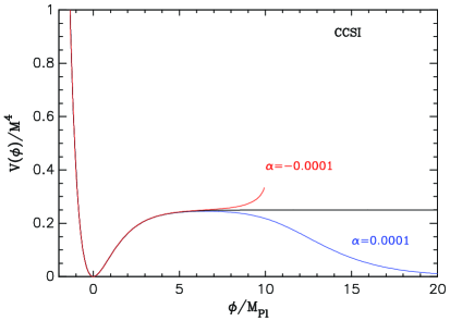
Figure 15: The potential (79) of the cubicly corrected Starobinsky model, for $\alpha>0$ ($\mathrm{CCSI}_{1}$) and $\alpha<0$ ($\mathrm{CCSI}_{3}$). The potential of Starobinsky inflation ($\mathrm{SI}$) is the middle plateau ($M^{4}\equiv M_{\scriptscriptstyle{\mathrm{Pl}}}^{2}\mu^{2}/2$).

In Sec. II.3, we have established that there is no fine-tuning issue for the initial conditions in the case of plateau inflation. The reason is clear: the presence of a large plateau in the potential ensures the relaxation of kination into slow roll according to Eq. (65). Physically, however, the plateau may not extend to infinitely large-field values due to the presence of higher-order corrections. This is noticed in Ref. Ijjas et al. (2013), which emphasizes that in the Taylor expansion of $V(\phi)$, the desired flat behavior can be obtained only if a precise cancellation order by order in $\phi$ occurs. Although there are mechanisms that automatically produce such an “exact” plateau, see e.g. Ref. Kallosh and Linde (2013), a legitimate question is then to determine whether UV-completed plateau models suffer from a fine-tuning problem.

Let us first notice that if the correction is of the large-field type, e.g., in a potential of the type

$$V(\phi) =V_{\mathrm{SI}}(\phi)\,{\Theta}\!\left(\frac{\phi_{\mathrm{corr}}}{M_{\scriptscriptstyle{\mathrm{Pl}}}}-\frac{\phi}{M_{\scriptscriptstyle{\mathrm{Pl}}}}\right)$$

$$+V_{\mathrm{SI}}(\phi_{\mathrm{corr}})\left[1-{\Theta}\!\left(\frac{\phi_{\mathrm{corr}}}{M_{\scriptscriptstyle{\mathrm{Pl}}}}-\frac{\phi}{M_{\scriptscriptstyle{\mathrm{Pl}}}}\right)\right]\left(\frac{\phi}{M_{\scriptscriptstyle{\mathrm{Pl}}}}\right)^{p},$$ (69)

where $V_{\mathrm{SI}}(\phi)$ is the Starobinsky potential of Eq. (63) and ${\Theta}\!\left(x\right)$ is the Heaviside function, no fine-tuning is required since neither the plateau branch at $\phi<\phi_{\mathrm{corr}}$ nor the large-field branch at $\phi>\phi_{\mathrm{corr}}$ suffers from a fine-tuning problem.

More generically otherwise, Eq. (65) shows that the plateau needs only to cover a field range larger than $\Delta\Phi_{\max}$ for relaxation to occur. Let us illustrate this property by considering the cubicly corrected Starobinsky model ($\mathrm{CCSI}$), which is a type of correction more physically motivated than the phenomenological form (II.5). It is a modified gravity $f(R)$ model given by Artymowski et al. (2015, 2016)

$$f(R)=R+\frac{R^{2}}{\mu^{2}}+\alpha\dfrac{R^{3}}{\mu^{4}}\,,$$ (70)

where $\mu$ is a mass scale and $\alpha$ an expected small dimensionless number. After a conformal transformation, any $f(R)$ theory can be cast into a scalar field theory, where the scalar field $\phi$ is defined as De Felice and Tsujikawa (2010)

$$\phi=\sqrt{\dfrac{3}{2}}\,M_{\scriptscriptstyle{\mathrm{Pl}}}\ln\left(\left|F\right|\right),$$ (71)

where

$$F(R)=\dfrac{\partial f(R)}{\partial R}=\exp{\left(\sqrt{\dfrac{2}{3}}\dfrac{\phi}{M_{\scriptscriptstyle{\mathrm{Pl}}}}\right)}.$$ (72)

The corresponding potential can be written as

$$V(\phi)=\frac{M_{\scriptscriptstyle{\mathrm{Pl}}}^{2}}{2}\,\frac{\left|F\right|}{F}\,\frac{R\,F-f}{F^{2}}\,.$$ (73)

Let us first consider the case where $\alpha=0$. Defining

$$y\equiv\sqrt{\dfrac{2}{3}}\dfrac{\phi}{M_{\scriptscriptstyle{\mathrm{Pl}}}}\,,$$ (74)

and solving Eq. (72) for $R$, one gets

$$R=\dfrac{\mu^{2}}{2}\left(e^{y}-1\right).$$ (75)

The potential (73) is then given by

$$V(\phi)=\frac{M_{\scriptscriptstyle{\mathrm{Pl}}}^{2}\,\mu^{2}}{8}\left(1-e^{-y}\right)^{2},$$ (76)

which, as expected, corresponds to the standard Starobinsky model of Sec. II.3. Therefore, the higher-order terms in Eq. (70) are natural gravity-motivated corrections to $\mathrm{SI}$. Notice that the potential of Starobinsky inflation matches the one of Higgs inflation Bezrukov and Shaposhnikov (2008), where one assumes that the inflaton field is the Higgs boson non minimally coupled to gravity. This picture could also motivate the form of other possible corrections Barvinsky et al. (2008); De Simone et al. (2009); Bezrukov et al. (2011).

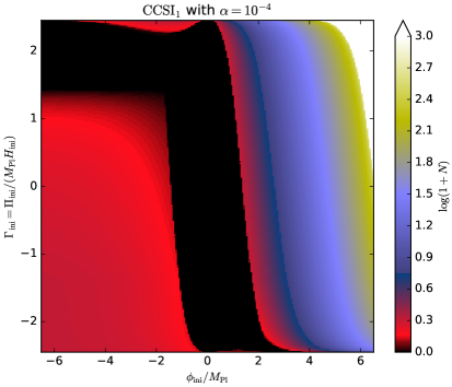
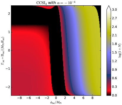
Figure 16: Number of e-folds of inflation for the $\mathrm{CCSI}_{1}$ ($\alpha>0$, upper panel) and $\mathrm{CCSI}_{3}$ ($\alpha<0$, lower panel) models along $2048^{2}$ phase-space trajectories. Even though the plateau is reduced compared to $\mathrm{SI}$, starting inflation does not require fine-tuning of the initial conditions. At large-field values, the number of e-folds is unbounded in $\mathrm{CCSI}_{1}$ while the UV cutoff ensures that it remains finite in $\mathrm{CCSI}_{3}$. The upper-right black corner in the lower panel corresponds to cases where the field climbs up the potential to $\phi_{\mathrm{uv}}$ where it stops being defined. In this case, the integration is stopped and the corresponding forbidden region is simply displayed in black.

Let us now consider the case where $\alpha$ is non-zero. Solving Eq. (72) for $R$ gives

$$1+2\dfrac{R}{\mu^{2}}+3\alpha\dfrac{R^{2}}{\mu^{4}}=e^{y},$$ (77)

whose roots are

$$R=\frac{\mu^{2}}{3\alpha}\left[-1\pm\sqrt{1+3\alpha\left(e^{y}-1\right)}\right].$$ (78)

We choose the positive sign in the above equation so that it reduces to the expression (75) for the standard Starobinsky model in the limit $\alpha\to 0$. With this solution, the potential reads

$$V(\phi) =\dfrac{M_{\scriptscriptstyle{\mathrm{Pl}}}^{2}\mu^{2}}{2}\left(1-e^{-y}\right)^{2}$$ (79)

$$\times\dfrac{1+\sqrt{1+3\alpha\left(e^{y}-1\right)}+2\alpha\left(e^{y}-1\right)}{\left[1+\sqrt{1+3\alpha\left(e^{y}-1\right)}\right]^{3}}\,,$$

which matches Eq. (63) for $\alpha=0$. For $\alpha>0$ ($\mathrm{CCSI}_{1}$), the potential is always well defined at large-field values. The plateau is distorted and there is a maximum at

$$\phi_{{}_{{\scriptscriptstyle{V}}^{\max}}}=\sqrt{\dfrac{3}{2}}M_{\scriptscriptstyle{\mathrm{Pl}}}\ln\left(\dfrac{2+4\sqrt{\alpha}}{\sqrt{\alpha}}\right),$$ (80)

above which the potential asymptotically goes to zero. For $\alpha<0$ ($\mathrm{CCSI}_{3}$), the potential is only defined for $\phi<\phi_{\mathrm{uv}}$, where

$$\phi_{\mathrm{uv}}=\sqrt{\frac{3}{2}}M_{\scriptscriptstyle{\mathrm{Pl}}}\ln\left(1-\dfrac{1}{3\alpha}\right).$$ (81)

At $\phi_{\mathrm{uv}}$, the potential is finite and its value is the one on the asymptotic plateau (when $\alpha=0)$ multiplied by $4/[3(1-3\alpha)^{2}]$.

The potentials of $\mathrm{CCSI}_{1}$ and $\mathrm{CCSI}_{3}$ have been represented in Fig. 15. Clearly, the correction breaks the infinitely wide plateau that was present in $\mathrm{SI}$. In Fig. 16, we have plotted the number of e-folds of inflation in phase-space for these two potentials. As expected, inflation still occurs in a large part of phase-space and no fine-tuning is required. These plots can be compared to Fig. 6. For $\mathrm{CCSI}_{1}$, there is almost no change compared to $\mathrm{SI}$, the whole large-field domain produces inflation. However, a crucial change is that the number of e-folds in the region $\phi>\phi_{{}_{{\scriptscriptstyle{V}}^{\max}}}$ is infinite and inflation never ends. For $\mathrm{CCSI}_{3}$ the situation is reversed. The field being bounded by $\phi<\phi_{\mathrm{uv}}$, the total number of e-folds of inflation can be large but never exceeds $10^{3}$.

Let us estimate how small the parameter $\alpha$ should be in order to have $\mathcal{N}_{\mathrm{inf}}$ e-folds of slow-roll plateau inflation. Approximating Eq. (64) in the large $\mathcal{N}_{\mathrm{inf}}$ regime, one has $\Phi_{\times}\simeq\sqrt{3/2}\ln(4\mathcal{N}_{\mathrm{inf}}/3)$. Requiring that $\phi_{{}_{{\scriptscriptstyle{V}}^{\max}}}>\Phi_{\times}M_{\scriptscriptstyle{\mathrm{Pl}}}$ in $\mathrm{CCSI}_{1}$ then leads to $\alpha<(2\mathcal{N}_{\mathrm{inf}}/3-2)^{-2}\simeq 10^{-3}$ for $\mathcal{N}_{\mathrm{inf}}\simeq 50$, and in $\mathrm{CCSI}_{3}$, the condition $\phi_{\mathrm{uv}}>\Phi_{\times}M_{\scriptscriptstyle{\mathrm{Pl}}}$ leads to $|\alpha|<1/(4\mathcal{N}_{\mathrm{inf}}-3)\simeq 5\times 10^{-3}$. No extreme fine-tuning is thus required on the small expansion parameter $\alpha$, and plateau inflation is therefore rather robust to small corrections that may eventually break the plateau.

II.6 Model simplicity

How natural the inflationary paradigm is can also be discussed by considering whether the data can be explained with simple models of inflation or if it forces us to consider more complicated and contrived scenarios. For instance, in Ref. Ijjas et al. (2013), it is argued that the models ruled out by Planck, like $\mathrm{LFI}_{4}$, are among the simplest ones since they require only one parameter, while “the plateau-like models require three or more parameters and must be fine-tuned”, hence are much less simple. In this section, we analyze this question.

Let us first notice that due to the non-detection of non-Gaussianities, isocurvature perturbations or departures from scale invariance, the minimal models of inflation relying on a single scalar field in the slow-roll regime, remain in excellent agreement with the data.

The main issue is then obviously in the definition of “simplicity” for a model. Even if one accepts the naive definition in terms of the number of free parameters, the Starobinsky model $\mathrm{SI}$ is as simple as, say $\mathrm{LFI}_{4}$, since both contain a single parameter and require only $\phi\gtrsim 5M_{\scriptscriptstyle{\mathrm{Pl}}}$ in order to have hundreds or more e-folds of inflation.

A more objective meaning to the concept of simplicity can be given in the Bayesian approach, which penalizes wasted parameter space and rewards models that achieve a good compromise between quality of fit and lack of fine-tuning. In this sense, plateau/hilltop inflation is no more complicated than large-field models, as shown in Ref. Martin et al. (2014b).

Let us also notice that parameters counting can be ambiguous. For instance, the same potential as in $\mathrm{SI}$ can be obtained from the Higgs field action non minimally coupled to gravity, the so-called Higgs-inflation model $\mathrm{HI}$ Bezrukov and Shaposhnikov (2008). In $\mathrm{HI}$, one might argue that more than one parameter is present: $\xi$, the non-minimal coupling to gravity and $\lambda$ the self-interacting Higgs coupling constant. They nonetheless combine into a single quantity $M^{4}=M_{\scriptscriptstyle{\mathrm{Pl}}}^{4}\lambda/(4\xi^{2})$ to produce the one-parameter potential of Eq. (63). The situation is exactly the same for $\mathrm{LFI}_{4}$: the potential is $V(\phi)=\lambda\phi^{4}$ but it can be justified from more fundamental theories containing several parameters that all combine to give $\lambda$. This is exactly what happens if one constructs supergravity (SUGRA) models of $\mathrm{LFI}$ as discussed in Sec. 4.2.1 of Ref. Martin et al. (2014a), see Eq. (4.33). So a one-parameter model in this context means a one-parameter model as far as CMB predictions are concerned.

We conclude that, at this stage, the data are perfectly compatible with the minimal and simplest implementations of inflation.

III Initial conditions beyond isotropy and homogeneity

The results discussed above assume that the universe is homogeneous and isotropic. This is evidently not satisfactory since inflation is precisely supposed to homogenize and isotropize the universe. This issue is clearly crucial for inflation and is part of the general problem of initial conditions. Technically, however, it is much more complicated than the problem treated in Sec. II.

III.1 Beyond isotropy

A first step toward a more complete investigation of this question is to maintain homogeneity and relax isotropy only and see whether inflation isotropizes the universe, see Refs. Steigman and Turner (1983); Anninos et al. (1991); Turner and Widrow (1986). This strategy can be exemplified by considering the Bianchi I metric which reads

$$\mathrm{d}s^{2}=-\mathrm{d}t^{2}+a_{i}^{2}(t)\left(\mathrm{d}x^{i}\right)^{2},$$ (82)

where each direction in space now has its own scale factor. The same metric can also be expressed as $\mathrm{d}s^{2}=-\mathrm{d}t^{2}+a^{2}(t)\gamma_{ij}\mathrm{d}x^{i}\mathrm{d}x^{j}$ with

$$a(t)\equiv\left[a_{1}(t)a_{2}(t)a_{3}(t)\right]^{1/3},$$ (83)

and

$$\gamma_{ij}=\begin{pmatrix}e^{2\beta_{1}(t)}&0&0\\ 0&e^{2\beta_{2}(t)}&0\\ 0&0&e^{2\beta_{3}(t)}\end{pmatrix},$$ (84)

with $\sum_{i=1}^{i=3}\beta_{i}=0$. As before, we assume the matter content of the early universe to be dominated by a scalar field $\phi(t)$, with a potential $V(\phi)$. Then, the Einstein equations lead to

$$3\frac{\mathcal{H}^{2}}{a^{2}} =\frac{1}{M_{\scriptscriptstyle{\mathrm{Pl}}}^{2}}\left[\frac{\phi^{\prime 2}}{2a^{2}}+V(\phi)\right]+\frac{\sigma^{2}}{2a^{2}},$$ (85)

$$-\frac{1}{a^{2}}\left(\mathcal{H}^{2}+2\mathcal{H}^{\prime}\right) =\frac{1}{M_{\scriptscriptstyle{\mathrm{Pl}}}^{2}}\left[\frac{\phi^{\prime 2}}{2a^{2}}-V(\phi)\right]+\frac{\sigma^{2}}{2a^{2}},$$ (86)

$$\left(\sigma^{i}_{j}\right)^{\prime}+2\mathcal{H}\sigma^{i}_{j} =0,$$ (87)

where $\mathcal{H}=a^{\prime}/a$, a prime denoting a derivative with respect to conformal time. In the above equation $\sigma_{ij}$ is the shear, defined as

$$\sigma_{ij}=\frac{1}{2}\gamma_{ij}^{\prime}=\begin{pmatrix}\beta_{1}^{\prime}e^{2\beta_{1}}&0&0\\ 0&\beta_{2}^{\prime}e^{2\beta_{2}}&0\\ 0&0&\beta_{3}^{\prime}e^{2\beta_{3}}\end{pmatrix},$$ (88)

and $\sigma^{2}=\sigma_{ij}\sigma^{ij}=\sum_{i=1}^{i=3}\beta_{i}^{\prime 2}$ with $\sigma^{i}_{j}=\gamma^{ik}\sigma_{kj}$. An isotropic universe corresponds to a vanishing shear. Indeed, if the $\beta_{i}$’s are constant, one can always redefine the spatial coordinates $x_{i}$ such that Eq. (82) reduces to the FLRW metric.

In order to study the dynamics of the system, one has to solve the Einstein equations (85), (86) and (87). This is especially easy for Eq. (87), which does not directly depend on $\phi(t)$. The corresponding solution is given by $\sigma^{i}_{j}=S^{i}_{j}/a^{2}$, where $S^{i}_{j}$ is a time-independent tensor. As a consequence, one has $\sigma^{2}=S^{2}/a^{4}$ where $S^{2}=S^{i}_{j}S^{j}_{i}$ is a constant. This implies that the shear is, in fact, equivalent to a stiff fluid with an equation-of-state parameter $w_{\sigma}\equiv p_{\sigma}/\rho_{\sigma}=1$ and energy density $\rho_{\sigma}=M_{\scriptscriptstyle{\mathrm{Pl}}}^{2}S^{2}/(2a^{6})$.

Two situations must then be considered. If $\rho_{\phi}\gg\rho_{\sigma}$ initially, then the universe inflates and quickly isotropizes since $\rho_{\sigma}\propto e^{-6N}$. If, on the contrary, the shear initially dominates, $\rho_{\sigma}\gg\rho_{\phi}$, then the universe expands as $a\propto t^{1/3}$ and the expansion is not accelerated. In that case, initially the field is slowly rolling, $\rho_{\phi}$ is approximately constant, and, since $\rho_{\sigma}\propto a^{-6}$, after a transitory period inflation starts and isotropizes the universe; or, the kinetic energy of the scalar field dominates over its potential energy, both $\rho_{\phi}$ and $\rho_{\sigma}$ decay as $\propto a^{-6}$, and once the potential energy becomes larger than the kinetic energy, inflation starts and also isotropizes the universe.

We conclude that, generically, inflation makes the universe isotropic, and the presence of initial shear is not a threat for inflation.

III.2 Beyond homogeneity

Despite the previous analysis, which is clearly a good point for inflation, the most difficult question remains to be addressed, namely whether inflation can homogenize the universe. Technically, this is a complex problem since one must now consider a situation that is initially inhomogeneous (and also anisotropic).

An analytical approach that has been used in the literature to investigate this problem is the so-called “effective-density approximation”, which was studied in Refs. Goldwirth and Piran (1990, 1992) (for different methods and/or arguments, see also Refs. Albrecht and Brandenberger (1985); Albrecht et al. (1985, 1987); Brandenberger (2016) and Refs. Vachaspati and Trodden (1999); Berera and Gordon (2001); Easther et al. (2014)). The idea is to consider an inhomogeneous scalar field on an isotropic and homogeneous FLRW background, assuming that the backreaction of the field inhomogeneities does not modify too much the FLRW metric, and manifests itself only via a new term in the Friedmann-Lemaître equation that simply changes the value of the Hubble parameter. Concretely, one takes

$$\phi(t,{\bm{x}})=\phi_{0}(t)+\Re\left[\delta\phi(t)e^{i{\bm{k}}\cdot{\bm{x}}/a(t)}\right],$$ (89)

and assumes that the corresponding Klein-Gordon equation can be split into two equations for the zero mode and for the inhomogeneous mode. This leads to

$$\ddot{\phi}_{0}+3H\dot{\phi}_{0}+V_{\phi}(\phi_{0}) =0,$$ (90)

$$\ddot{\delta\phi}+3H\dot{\delta\phi}+\frac{k^{2}}{a^{2}}\delta\phi =0.$$ (91)

Let us notice that, despite the notation, $\delta\phi(t)$ needs not be small compared to $\phi_{0}(t)$. The crucial ingredient of this approximation scheme is that, in Eq. (91), the potential does not appear. We therefore assume that the length scale of the inhomogeneities is small enough for the potential energy to be negligible compared to the gradients. As mentioned above, the Friedmann-Lemaître equation is then expressed as

$$H^{2}=\frac{1}{3M_{\scriptscriptstyle{\mathrm{Pl}}}^{2}}\left[\frac{1}{2}\dot{\phi}_{0}^{2}+V(\phi_{0})+\frac{1}{2}\dot{\delta\phi}^{2}+\frac{1}{2}\frac{k^{2}}{a^{2}}\delta\phi^{2}\right]-\frac{{\mathcal{K}}}{a^{2}}.$$ (92)

This approximation should be valid if the wavenumber ${\bm{k}}$ is such that the wavelength of the inhomogeneous part is much smaller than the Hubble radius, namely $k\gg aH$, see Refs. Goldwirth and Piran (1990, 1992). If, on the contrary, it is much larger than the Hubble radius, then this should just amount to a normalization of the homogeneous field in our local Hubble volume. In this framework, the energy density of the inhomogeneities is defined by $\rho_{\delta\phi}=\rho_{\dot{\delta\phi}}+\rho_{\nabla}$, with $\rho_{\dot{\delta\phi}}=\dot{\delta\phi}^{2}/2$ and $\rho_{\nabla}=k^{2}\delta\phi^{2}/(2a^{2})$ while the energy density of the homogeneous mode is, as usual, given by $\rho_{\phi_{0}}=\dot{\phi}_{0}^{2}/2+V(\phi_{0})$. Then, the problem can be reformulated in the following way: if, initially, $\rho_{\delta\phi}\gg\rho_{\phi_{0}}$, namely if initially the universe is strongly inhomogeneous, then can $\rho_{\delta\phi}$ decrease such that $\rho_{\phi_{0}}$ takes over and inflation starts, thus making the universe homogeneous?

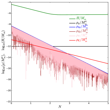
Figure 17: Evolution of the Hubble parameter and of the various energy densities obtained by numerical integration of Eqs. (90), (91) and (92). The potential is chosen to be the Starobinsky one, see Eq. (63) with a scale $M=0.001M_{\scriptscriptstyle{\mathrm{Pl}}}$, which, roughly speaking, matches the CMB normalization. The initial value of the field is $\phi_{0}=6M_{\scriptscriptstyle{\mathrm{Pl}}}$ and the initial velocity is taken to be $\dot{\phi}_{0}=-V_{\phi}(\phi_{0})/[3V(\phi_{0})]$ (which is the slow-roll velocity). In the absence of inhomogeneities, with these initial conditions, inflation would start and would lead to more than $\simeq 100$ e-folds. The initial value of $\delta\phi$ is taken to be $0.01M_{\scriptscriptstyle{\mathrm{Pl}}}$ (and is therefore less than the Planck mass as required, see the main text) while the initial velocity of $\delta\phi(t)$ is given by $\dot{\delta\phi}_{\mathrm{ini}}=0$. The scale $k$ is chosen to be $k/a_{\mathrm{ini}}=10^{-2}M_{\scriptscriptstyle{\mathrm{Pl}}}$ and the initial curvature has been set to $\rho_{\mathcal{K}}=-5\times 10^{-11}\,M_{\scriptscriptstyle{\mathrm{Pl}}}^{4}$. This implies that $H_{\mathrm{ini}}/M_{\scriptscriptstyle{\mathrm{Pl}}}\simeq 4\times 10^{-5}$, $\rho_{\phi,{\mathrm{ini}}}\simeq 10^{-12}M_{\scriptscriptstyle{\mathrm{Pl}}}^{4}$, and $\rho_{\delta\phi,{\mathrm{ini}}}\simeq 5\times 10^{-9}M_{\scriptscriptstyle{\mathrm{Pl}}}^{4}$. Those initial conditions are such that $H_{\mathrm{ini}}^{2}a_{\mathrm{ini}}^{2}/k^{2}\simeq 1.66\times 10^{-5}\ll 1$ and $\rho_{\phi,{\mathrm{ini}}}/\rho_{\delta\phi,{\mathrm{ini}}}\simeq 2\times 10^{-4}$, namely the inhomogeneities largely dominate initially.

Initially, we can choose $\dot{\phi}_{0}$ and $\phi_{0}$ such that, in the absence of inhomogeneities, slow-roll inflation would start (therefore, those values depend on the potential that we assume). If, initially, the inhomogeneities dominate, then Eq. (92) can be expressed as $H^{2}\simeq\rho_{\delta\phi}/(3M_{\scriptscriptstyle{\mathrm{Pl}}}^{2})$, or

$$\frac{3a^{2}H^{2}}{k^{2}}\simeq\frac{1}{2}\frac{\dot{\delta\phi}^{2}}{M_{\scriptscriptstyle{\mathrm{Pl}}}^{2}}\frac{a^{2}}{k^{2}}+\frac{1}{2}\frac{\delta\phi^{2}}{M_{\scriptscriptstyle{\mathrm{Pl}}}^{2}}.$$ (93)

One can also include a non-vanishing initial curvature, but as long as $\mathcal{K}$ is not large enough to make the universe collapse, its effects quickly disappear (see the red line in Fig. 17). However, we stress that, if the initial curvature is much larger, this picture could be drastically modified. As a matter of fact, we have checked that, if one increases its contribution by one order of magnitude, the values of the other parameters used in Fig. 17 being otherwise the same, then the universe recollapses. Therefore, if it is not necessary to assume that curvature is initially tiny, it is nevertheless true that it should be subdominant. This is the hypothesis that we make in the following and this is the reason why it is ignored in the above equation. Then, the condition that the wavelength of the inhomogeneities is smaller than the Hubble radius implies that the left-hand side of Eq. (93) is small. This results in the following initial conditions: $\delta\phi\ll M_{\scriptscriptstyle{\mathrm{Pl}}}$ and $\dot{\delta\phi}^{2}/M_{\scriptscriptstyle{\mathrm{Pl}}}^{2}\ll k^{2}/a^{2}$.

In Fig. 17, we have numerically integrated Eqs. (90), (91) and (92). Initially, we see that $\rho_{\delta\phi}\gg\rho_{\phi}$, namely the universe is strongly inhomogeneous. Then, $\rho_{\dot{\delta\phi}}$ (brown line) and $\rho_{\nabla}$ (pink line) and, therefore, $\rho_{\delta\phi}$, decrease (blue line) as $a^{-4}$ while $\rho_{\phi}$ is approximately constant. During this phase, the Hubble parameter is not constant and we do not have inflation.

The fact that $\rho_{\delta\phi}$ behaves as radiation can be understood from noticing that

$$\delta\phi(t)\simeq\Re\left[\delta\phi_{\mathrm{ini}}\frac{a_{\mathrm{ini}}}{a(t)}e^{i\frac{k}{a_{\mathrm{ini}}H_{\mathrm{ini}}}\frac{a(t)}{a_{\mathrm{ini}}}}\right],$$ (94)

provides a solution to Eqs. (91) and (93) in that case. This implies that, very quickly, $\rho_{\phi}$ takes over, the universe becomes homogeneous, the Hubble parameter settles to a constant and inflation starts. In this regime, Eqs. (91) still possesses an analytical solution, given by

$$\delta\phi(t)\simeq\Re\left[\delta\phi_{\mathrm{ini}}\frac{a_{\mathrm{ini}}}{a(t)}e^{i\frac{k}{a_{\mathrm{ini}}H_{\mathrm{ini}}}\frac{a_{\mathrm{ini}}}{a(t)}}\right],$$ (95)

at leading order in $aH/k$. At that order, this implies that $\rho_{\delta\phi}$ still decays as $1/a^{4}$ during inflation, as can be checked in Fig. 17. This is the case until $k$ crosses out the Hubble radius, at which point the entire effective-density approximation scheme breaks down.

We have reproduced the above analysis for the Coleman-Weinberg potential, see Eq. (68) for $Q=10^{-3}M_{\scriptscriptstyle{\mathrm{Pl}}}$ and found the same qualitative behavior (the same result was also found for LFI models), which seems to indicate that it is independent of the potential chosen, in agreement with Refs. Goldwirth and Piran (1990, 1992).

We conclude that, in the previous setting, the presence of large inhomogeneities cannot prevent inflation. However, as also stressed in Refs. Goldwirth and Piran (1990, 1992), this conclusion is obtained assuming the size of the inhomogeneities to be much smaller than the Hubble radius. This means that the previous results are, in fact, limited and have a small impact on our general understanding of how the universe becomes homogeneous during inflation. As a matter of fact, in the most general situation (in particular if the size of the inhomogeneous mode is of the order of the Hubble radius), only a numerical integration of the full Einstein equations can provide a correct answer.

This has been carried out by several authors. The first numerical solutions Goldwirth and Piran (1990, 1989, 1992); Goldwirth (1991) were obtained under the assumption that spacetime is spherically symmetric. This simplifies the calculations since then the problem only depends on time and on one radial coordinate. Nevertheless, the Einstein equations remains partial (as opposed to ordinary as in the situation treated before) non-linear differential equations. This analysis was improved in Refs. Kurki-Suonio et al. (1987); Laguna et al. (1991); Kurki-Suonio et al. (1993) in which the spherical symmetry assumption was relaxed. More recently, Refs. East et al. (2016); Clough et al. (2017); Bloomfield et al. (2019) have run new simulations (and seem to confirm the validity of the behavior $\rho_{\delta\phi}\propto a^{-4}$ found above, even when $k\sim aH$). All these works have technical restrictions and, at this stage, it is difficult to draw a completely general conclusion. However, it seems that LFI and plateau models work better than SFI, and that although the size of the initial homogeneous patch is an important parameter of the problem, strong gradients may also help in starting inflation (see also Refs. Calzetta and Sakellariadou (1992); Perez and Pinto-Neto (2011)).

It is also worth mentioning that, speculating on what Quantum Gravity could be, it does not seem unreasonable to assume that a patch of Planck size should be homogeneous. If this patch can be stretched to the observable universe today, then the homogeneity problem would be solved. However, without inflation, this is not possible. Indeed, in the hot big bang model, the Planck energy density is reached at redshift $z_{\mathrm{Pl}}\simeq 10^{30}$. The Planck length, $\ell_{\mathrm{Pl}}\simeq 10^{-35}\,\mathrm{m}$, at this initial redshift, is thus stretched to $\simeq 10^{-5}\,\mathrm{m}$ today, to be compared to the Hubble radius today, $r_{\mathrm{H}}\simeq 10^{26}\,\mathrm{m}$. This is a generic feature of decelerated expansion, which redshifts length scales by an amount always smaller than the increase of the Hubble radius. But, on the contrary, with a sufficient number of inflationary e-folds, the initial Planck patch becomes larger than the Hubble patch today and, within the above-mentioned hypothesis, the homogeneity problem is solved. Notice that this does not address, within Quantum Gravity, the problem of starting inflation, which is a topic by itself Linde (1984, 1985); Coule and Martin (2000).

We conclude that the fundamental issue as to whether inflation homogenizes the universe is still open, although most recent numerical works on this topic seem to be suggesting it does. Among all the potential problems that have been raised against inflation, it is clearly the most serious one.

IV The Trans-Planckian Problem

In the previous sections, we studied how inflation depends on initial conditions. A similar question exists for the perturbations. In fact, if one traces backwards in time the length scales of cosmological interest today, they are generically smaller than the Planck length at the onset of inflation. It is in this regime that the initial conditions (the adiabatic vacuum) are chosen. But one can wonder whether this is legitimate and whether quantum field theory in curved spacetime is valid in this case. Notice that the energy density of the background remains much less than the Planck energy density, so that the use of a classical background is well justified, and it is only the wavelengths of the perturbations that can be smaller than the Planck length. This issue is known as the trans-Planckian problem of inflation Martin and Brandenberger (2001); Brandenberger and Martin (2001, 2013, 2005).

In absence of a final theory of quantum gravity, it is difficult to calculate what would be the modifications to the behavior of the perturbations if physics beyond the Planck scale were taken into account. But what can be done is to introduce several ad hoc but reasonable modifications and test whether the inflationary predictions are robust Martin and Brandenberger (2001); Brandenberger and Martin (2001) under those.

It has been shown that the inflationary power spectrum can be modified if physics is not adiabatic beyond the Planck scale. So, to a certain extent, the predictions are not robust. However, if one uses the most conservative way of modeling the modifications originating from the spacetime foam, one finds that the corrections scale as $(H/M_{\mathrm{c}})^{p}$, where $H$ is the Hubble scale during inflation and $M_{\mathrm{c}}$ the energy scale at which new physical effects pop up (typically the Planck scale or, possibly, the string scale); $p$ is an index which, in some cases, can simply be one Martin and Brandenberger (2003). Those corrections are therefore typically small. In some sense, this result can be viewed as decoupling between the Planck and inflationary scales. However, there are other ways of modeling the new physics (for instance, for some choices of modified dispersion relations Martin and Brandenberger (2002)) that could lead to more drastic modifications.

Notice that the form of these corrections is somehow generic. Choosing the adiabatic vacuum consists in singling out a specific Wentzel-Kramers-Brillouin (WKB) branch in the evolution of the cosmological perturbations, which is a second order differential equation. Any deviation from this will necessarily introduce interferences with the other branch and, as a result, superimposed oscillations will appear in the inflationary correlation functions Brandenberger and Martin (2002). Although the amplitude and the frequency of those oscillations are model dependent, their presence have been searched for in the CMB data but no conclusive signal has been found so far Martin and Ringeval (2004a); Martin and Ringeval (2005); Martin and Ringeval (2004b); Martin and Ringeval (2006).

In conclusion, it is fair to say that trans-Planckian effects are, at least in their most conservative formulations, not a threat for inflation. On the contrary, they should be viewed as a window of opportunity Martin and Brandenberger (2000); Easther et al. (2001): if we are lucky enough, one might use them to probe the Planck scale, something that would clearly be impossible with other means Martin and Brandenberger (2001); Brandenberger and Martin (2001); Easther et al. (2002); Armendariz-Picon and Lim (2003); Brandenberger and Martin (2005); Easther et al. (2005); Brandenberger and Martin (2013).

V Inflation and the Quantum Measurement Problem

The inflationary mechanism for structure formation is based on General Relativity and Quantum Mechanics. As a consequence, the behavior of inflationary perturbations is described by the Schrödinger equation that controls the evolution of their wavefunction. Initially, the system is placed in its ground state, which is a coherent state, and then, due to the expansion of spacetime, it evolves into a very peculiar state, namely a two-mode squeezed state. This state is sometimes described as “classical” since most of the corresponding quantum correlation functions can be obtained using a classical distribution in phase-space Polarski and Starobinsky (1996); Kiefer et al. (1998); Martin and Vennin (2016a). However, it also possesses properties usually considered as highly non classical. It is indeed an entangled state, very similar to the Einstein-Podolsky-Rosen (EPR) state, with a large quantum discord Martin and Vennin (2016a), which allows one to construct observables for which the Bell inequality is violated Martin and Vennin (2016b); Martin and Vennin (2017).

The above picture, however, raises an issue Sudarsky (2011); Goldstein et al. (2015): the quantum state of the perturbations is not an eigenstate of the temperature fluctuation operator. A non-unitary process needs therefore to be invoked, during which the state evolves from the two-mode squeezed state into an eigenstate of $\widehat{\delta T}/T$. In other words, the quantum state of the perturbations is homogeneous and something is needed to project it onto a state that contains inhomogeneities.

This problem is no more than the celebrated measurement problem of Quantum Mechanics, which, in the Copenhagen approach, is “solved” by the collapse of the wavefunction. In the context of Cosmology, however, the use of the Copenhagen interpretation appears to be problematic Hartle et al. (2019). Indeed, it requires the existence of a classical domain, exterior to the system, which performs a measurement on it. In quantum cosmology for instance, one calculates the wavefunction of the entire Universe and there is, by definition, no classical exterior domain at all. In the context of inflation, one could argue that the perturbations do not represent all degrees of freedom and that some other classical degrees of freedom could constitute the exterior domain, but they do not qualify as “observers” in the Copenhagen sense. The transition to an eigenstate of the temperature fluctuation operator, which necessarily occurred in the early Universe (structure formation started in the early Universe), thus proceeded in the absence of any observer, something at odds with the Copenhagen interpretation.

How is this problem usually addressed? One possibility is to resort to the many-world interpretation together with decoherence Kiefer et al. (2007). It can also be understood if one uses alternatives to the Copenhagen interpretation such as “collapse models”; see Refs. Perez et al. (2006); De Unanue and Sudarsky (2008); Leon and Sudarsky (2010); Martin et al. (2012); Cañate et al. (2013); Das et al. (2013). In this case, one obtains different predictions that can be confronted with CMB measurements. Other solutions involve the Bohmian interpretation of Quantum Mechanics Peter et al. (2007); Pinto-Neto et al. (2012); Peter and Vitenti (2016).

In conclusion, let us stress that the quantum measurement problem is present in quantum mechanics itself and is not specific to inflation: any mechanism where cosmological structures originate from quantum fluctuations would have to face it. As for the trans-Planckian problem, inflation can, however, be viewed as a window of opportunity that could shed light on fundamental issues of Quantum Mechanics using astrophysical measurements.

VI The Likelihood of Inflation

Another class of criticisms against inflation is based on the idea that there exists a natural measure on the space of classical universes and that, according to this measure, the probability of having a sufficient number of e-folds of slow-roll inflation is tiny. In this section, we examine these arguments.

The main idea is the following. Let us consider a system having $n$ degrees of freedom $q_{i}$ and described by the Hamiltonian $\mathscr{H}(q_{i},p_{i})$ where $p_{i}=-\partial\mathscr{H}/\partial q_{i}$ is the conjugate momentum of $q_{i}$. The evolution of the system can be followed in the $2n$-dimensional phase-space endowed with the coordinates $(q_{i},p_{i})$. Then, there exists a natural symplectic form given by $\omega=\sum_{i=1}^{n}\mathrm{d}p_{i}\wedge\mathrm{d}q_{i}$ which leads to the Liouville measure, namely $\Omega=(-1)^{n(n-1)/2}/n!\,\omega^{n}$. This measure is commonly and successfully used in statistical physics.

In the context of inflation, where gravity is relevant, one can also describe the system in terms of a Hamiltonian and, therefore, attempt to define a natural measure. Indeed, the Einstein-Hilbert action, in the homogeneous case, leads to the mini superspace Lagrangian

$$\mathcal{L}=-3\frac{M_{\scriptscriptstyle{\mathrm{Pl}}}^{2}}{\mathcal{N}}a\dot{a}^{2}+3\mathcal{N}M_{\scriptscriptstyle{\mathrm{Pl}}}^{2}\mathcal{K}a+\frac{a^{3}\dot{\phi}^{2}}{2\mathcal{N}}-\mathcal{N}a^{3}V(\phi).$$ (96)

Here, $\mathcal{N}$ is the lapse and plays the role of a Lagrange multiplier. The conjugate momenta read

$$p_{\mathcal{N}}=0,\qquad p_{a}=-6M_{\scriptscriptstyle{\mathrm{Pl}}}^{2}\dfrac{a\dot{a}}{\mathcal{N}},\qquad p_{\phi}=a^{3}\dfrac{\Pi}{\mathcal{N}}\,.$$ (97)

Performing a Legendre transform, one obtains the Hamiltonian

$$\mathscr{H}=\mathcal{N}\left[-\frac{p_{a}^{2}}{12M_{\scriptscriptstyle{\mathrm{Pl}}}^{2}a}+\frac{p_{\phi}^{2}}{2a^{3}}-3M_{\scriptscriptstyle{\mathrm{Pl}}}^{2}\mathcal{K}a+a^{3}V\left(\phi\right)\right].$$ (98)

The equation of motion for $\mathcal{N}$ sets it to be a constant, and the variation of the Lagrangian with respect to $\mathcal{N}$ gives the Friedmann-Lemaître equation (1) provided $\mathcal{N}=1$, which we choose to be the case in what follows. The Hamiltonian equation of motion for $\phi$ is nothing but the Klein-Gordon equation (3), while the Hamiltonian equation of motion for $a$, combined with the Friedmann-Lemaître equation, gives the Raychaudhuri equation (2). In practice, the Friedmann-Lemaître equation can be deduced from the Klein-Gordon and Raychaudhuri equations up to an integration constant (which corresponds to fixing $\mathcal{N}$).

As a result, the dynamics is effectively Hamiltonian on a four-dimensional phase-space $(\phi,p_{\phi},a,p_{a})$ and this can motivate the choice of the simplectic form

$$\omega_{{}_{\scriptscriptstyle{\mathrm{GHS}}}}=\mathrm{d}p_{a}\wedge\mathrm{d}a+\mathrm{d}p_{\phi}\wedge\mathrm{d}\phi.$$ (99)

The associated measure is known as the Gibbons-Hawking-Stewart (GHS) measure Gibbons et al. (1987).

At this point however, a first difficulty arises. Since General Relativity is a constrained setup, the physical system lives in fact on the surface $\mathscr{H}=0$ and not in the entire four-dimensional phase space. One can nevertheless consider the measure induced by the GHS form when pullbacked on this surface, which reads

$$\omega_{{\scriptscriptstyle{\mathrm{GHS}}},\mathscr{H}=0} =-6M_{\scriptscriptstyle{\mathrm{Pl}}}^{2}a^{2}\mathrm{d}H\wedge\mathrm{d}a$$ (100)

$$+\frac{6M_{\scriptscriptstyle{\mathrm{Pl}}}^{2}a^{3}H}{\sqrt{6H^{2}M_{\scriptscriptstyle{\mathrm{Pl}}}^{2}-2V(\phi)+\dfrac{6M_{\scriptscriptstyle{\mathrm{Pl}}}^{2}\mathcal{K}}{a^{2}}}}\mathrm{d}H\wedge\mathrm{d}\phi$$

$$+\frac{3a^{2}\left(6H^{2}M_{\scriptscriptstyle{\mathrm{Pl}}}^{2}-2V(\phi)+\dfrac{4M_{\scriptscriptstyle{\mathrm{Pl}}}^{2}\mathcal{K}}{a^{2}}\right)}{\sqrt{6H^{2}M_{\scriptscriptstyle{\mathrm{Pl}}}^{2}-2V(\phi)+\dfrac{6M_{\scriptscriptstyle{\mathrm{Pl}}}^{2}\mathcal{K}}{a^{2}}}}\mathrm{d}a\wedge\mathrm{d}\phi.$$

As detailed in Ref. Schiffrin and Wald (2012), this measure is still not satisfactory because it is degenerate, namely the determinant of $\omega_{{\scriptscriptstyle{\mathrm{GHS}}},\mathscr{H}=0}$ vanishes, and, as a consequence, it cannot lead to a correct volume form. In order to fix this second problem, the usual procedure consists in restricting the natural measure, not to the constraint surface itself, but to a surface within the constraint surface, $\mathscr{S}(N,H,\phi)=K_{*}$, which intersects each trajectory only once. By considering different values of $K_{*}$, one describes a succession of surfaces in the constraint surface, which can be viewed as describing the “passage of time”. The standard choice is to define $\mathscr{S}$ by $H=H_{*}$, which leads to the form introduced by Gibbons and Turok in Ref. Gibbons and Turok (2008), namely

$$\omega_{{\scriptscriptstyle{\mathrm{GHS}}},\mathscr{H}=0,H=H_{*}} =3a^{2}$$ (101)

$$\kern-10.00002pt\times\dfrac{6H_{*}^{2}M_{\scriptscriptstyle{\mathrm{Pl}}}^{2}-2V(\phi)+\dfrac{4M_{\scriptscriptstyle{\mathrm{Pl}}}^{2}\mathcal{K}}{a^{2}}}{\sqrt{6H_{*}^{2}M_{\scriptscriptstyle{\mathrm{Pl}}}^{2}-2V(\phi)+\dfrac{6M_{\scriptscriptstyle{\mathrm{Pl}}}^{2}\mathcal{K}}{a^{2}}}}\mathrm{d}a\wedge\mathrm{d}\phi.$$

This measure, however, suffers from a number of drawbacks as underlined in Ref. Schiffrin and Wald (2012). As discussed in great detail in Sec. III of this reference, in statistical physics, the use of the natural symplectic form is justified only if some conditions are satisfied. Reference Schiffrin and Wald (2012) shows that, in the context of inflation, none of these conditions is actually fulfilled. The physical motivations behind the GHS measure seem therefore elusive. Moreover, the measure (101) is, in fact, infinite and needs to be regularized. As discussed in Ref. Schiffrin and Wald (2012), the physical conclusions that one may draw unfortunately depend on the regularization scheme, and no universal scheme has been found so far. A common procedure is to introduce a cutoff $a_{\mathrm{c}}$ in $a$ and to take the limit $a_{\mathrm{c}}\to\infty$. Then, the probability of having slow-roll inflation lasting at least $\mathcal{N}_{\mathrm{inf}}$ e-folds is given by

$$P(\mathcal{N}_{\mathrm{inf}})=\dfrac{\displaystyle\int_{\mathcal{D}(\Phi_{\mathrm{ini}},\mathcal{N}_{\mathrm{inf}})}\sqrt{6H_{*}^{2}M_{\scriptscriptstyle{\mathrm{Pl}}}^{2}-V(\phi)}\,\mathrm{d}\phi}{\displaystyle\int\sqrt{6H_{*}^{2}M_{\scriptscriptstyle{\mathrm{Pl}}}^{2}-V(\phi)}\,\mathrm{d}\phi},$$ (102)

in agreement with Eq. (62) of Ref. Schiffrin and Wald (2012). In the numerator, the $\phi$ integral is taken for initial values of the inflaton leading to at least $\mathcal{N}_{\mathrm{inf}}$ e-folds and for values of $\phi$ such that the square root is defined, the corresponding integration domain being denoted by $\mathcal{D}(\Phi_{\mathrm{ini}},\mathcal{N}_{\mathrm{inf}})$. In the denominator, the range of integration comprises all values such that the square root is defined. Finally, we have also assumed flat spacelike sections, namely $\mathcal{K}=0$.

Then comes the question of which value of $H_{*}$ should be taken. The choice made in Ref. Gibbons and Turok (2008) is to choose $H_{*}$ as the Hubble parameter at the end of inflation from which one obtains [see also Ref. Schiffrin and Wald (2012), Eq. (69)]

$$P(\mathcal{N}_{\mathrm{inf}})\propto e^{-3\mathcal{N}_{\mathrm{inf}}}.$$ (103)

This result is at the origin of the claim that inflation is extremely unlikely. It is, however, tightly related to the choice of taking $H_{*}$ at the end of inflation, see Refs. Schiffrin and Wald (2012); Corichi and Sloan (2014): since slow roll is an attractor in phase-space, it is clear that, measured at the end of inflation, the volume occupied by the inflationary trajectories is very small.

The presence of a dynamical attractor is, in fact, a positive feature of inflation, as revealed by the result obtained when taking $H_{*}$ “initially”, say, at the Planck scale (or at scales slightly below if one wants to avoid quantum gravity effects). This choice seems better justified and leads to a completely different result. If one takes $V(\phi)=m^{2}\phi^{2}/2$, then Refs. Carroll and Tam (2010); Schiffrin and Wald (2012) have shown that

$$P(\mathcal{N}_{\mathrm{inf}})\simeq 1-\frac{4m}{\pi H_{*}}\sqrt{\dfrac{2\mathcal{N}_{\mathrm{inf}}}{3}},$$ (104)

which leads to $P(60)\simeq 0.99996$, namely sufficient inflation is almost certain. This number, however, depends on the potential. For instance, it has also been evaluated for Natural Inflation in Ref. Carroll and Tam (2010) which finds $P(60)\simeq 0.171$. Given the Planck CMB data, what should be done is to carry out this calculation for the best inflationary scenarios, namely the plateau single-field potentials such as the Starobinsky model. Using Eq. (63) together with Eq. (64) expanded in the large-$\Phi$ limit, one arrives at

$$P(\mathcal{N}_{\mathrm{inf}})=\frac{\displaystyle\int_{\ln(4\mathcal{N}_{\mathrm{inf}}/3)}^{\infty}\mathrm{d}x\sqrt{1-\mathscr{A}\left(1-e^{-x}\right)^{2}}}{\displaystyle\int_{0}^{\infty}\mathrm{d}x\sqrt{1-\mathscr{A}\left(1-e^{-x}\right)^{2}}},$$ (105)

where $\mathscr{A}$ is a dimensionless quantity given by

$$\mathscr{A}\equiv\frac{M^{4}}{6H_{*}^{2}M_{\scriptscriptstyle{\mathrm{Pl}}}^{2}}.$$ (106)

The upper limit of the integral is infinite because, in a plateau model, $6H_{*}^{2}M_{\scriptscriptstyle{\mathrm{Pl}}}^{2}-V(\phi)$ is, in the slow-roll approximation, always positive regardless of $\phi$. The two integrals present in the ratio (105) are infinite, but they can be regularized by replacing the upper infinite limit with a finite cutoff $x_{\mathrm{sup}}$, upon which they behave as $\sim\sqrt{1-\mathscr{A}}\,x_{\mathrm{sup}}$. Letting $x_{\mathrm{sup}}\rightarrow\infty$, one then simply obtains $P(\mathcal{N}_{\mathrm{inf}})=1$. Therefore, if one were ready to accept the previous considerations (with all the caveats mentioned), the conclusion would be that Planck has precisely singled out the models for which the probability of getting enough e-folds of inflation is unity, and that would rather reinforce the status of inflation. Let us also notice that Ref. Ijjas and Steinhardt (2016) has remarked that the use of the Liouville measure in the cosmological context is often disputed but has argued that any other approaches lead the same conclusions. The previous considerations, however, show that it is sufficient to take a reasonable value for $H_{*}$ to completely change the consequences.

Let us quickly review the results obtained in this section. The claim that inflation is unlikely, which is expressed mathematically by Eq. (103), is based on the use of the GHS measure which, contrary to the case of statistical physics, does not satisfy any of the conditions required for the validity of the Liouville measure Schiffrin and Wald (2012). This measure therefore lacks physical justifications, as other proposed measures in the literature Finn and Karamitsos (2019). If one were to use it anyway, the result would strongly depend on the regularization scheme. If one further insists and employs one such scheme where a cutoff on the scale factor is introduced, if one chooses $H_{*}$ at the beginning of inflation rather than at the end, one finds that sufficient inflation is very likely (and even certain for the plateau models that seem to emerge from the data) rather than unlikely. This is due to the presence of a dynamical attractor, namely slow roll, and leads us to conclude that the claim that inflation is unlikely can safely be discarded.

VII Initial Conditions, Attractors and Measures

The discussion in Sec. II about fine-tuning in the space of initial conditions is crucially based on the existence of an attractor, which appears to be a fundamental property of inflation. However, as was emphasized in Ref. Remmen and Carroll (2013), the presence of an attractor during inflation can be challenged. First, there is the Liouville theorem, which states that volumes are conserved in phase-space and goes against the intuitive meaning of what an attractor is. Second, an attractor is a coordinate-dependent notion.

Concerning this second point, it was shown in Sec. II that there is a convergence of inflationary trajectories toward the slow-roll trajectory when plotted in the coordinates $(\phi,\Pi)$ or $(\Phi,\Gamma)$. However, as noticed in Ref. Remmen and Carroll (2013), if the same trajectories are represented in terms of the coordinates $(\phi,p_{\phi})$, the attractor behavior is lost (see Fig. 2 of Ref. Remmen and Carroll (2013)). The reason is that $p_{\phi}$ is related to $\dot{\phi}$ by a time-dependent function, namely $a^{3}$ as can be seen in Eqs. (97), and that, as we will see, the rate at which trajectories approach the slow-roll attractor is precisely given by $1/a^{3}$. In fact, the attractor behavior of any system (not necessarily in Cosmology) obtained with given coordinates can always be erased by changing these coordinates, in particular by suitably multiplying them by some time-dependent function. The presence of an attractor, and, hence, the sensitivity to initial conditions, is therefore intimately related to the choice of a measure in phase space.

In fact, among the measures that can be proposed, two categories can be distinguished. The first category corresponds to measures that can be written as $f(x,y)\mathrm{d}x\wedge\mathrm{d}y$, where $x$ and $y$ parametrize phase-space and obey $\mathrm{d}x/\mathrm{d}\tau=X(x,y)$ and $\mathrm{d}y/\mathrm{d}\tau=Y(x,y)$ (here $\tau$ denotes the time label used to formulate the equations of motion), namely the equation of motion are autonomous, that is to say they do not explicitly depend on $\tau$. The second category contains measures that are not of type I, either because $f$ explicitly depends on the time label $\tau$, or because the equations of motion are not autonomous, or both. Measures of category II are a priori not well-defined unless, using some additional prescription, one can reexpress the time label in terms of the dynamical variables of the system.

In this section, we discuss alternatives to the flat measure in $(\Phi,\Gamma)$ implicitly assumed in Sec. II, their motivations, and their relevance for characterizing dynamical attractors and the fine-tuning of initial conditions. We will specify the category (I or II) of each measure and show that the presence of an attractor is always found with measures of category I.

VII.1 Alternative measures

Let us introduce several measures that can be viewed as “natural”. Our goal is by no means to be exhaustive (one probably could define other measures) or to argue that one measure is better than the others. The aim is rather to show that the notion of an inflationary attractor is robust in the sense that, given reasonable measures, and for various attractor criteria, it is almost always present.

VII.1.1 Field-space $t$-measure

Since Eqs. (1) and (3) give rise to a closed, time-independent differential system in the space $(\phi,\Pi)$, where we recall that $\Pi=\dot{\phi}$, a first natural choice for a measure is one that is flat in this space, $\mathrm{d}\phi\wedge\mathrm{d}\Pi$. Because this comes from parametrizing trajectories with cosmic time $t$ (in other words the time label $\tau$ is $\tau=t$), we will refer to this as the $t$-measure. This measure clearly belongs to category I because the function $f$ does not depend on time (it is one) and the equations of motion are, as just noticed above, autonomous since $\dot{\phi}=\Pi$ and $\dot{\Pi}=-3[\Pi^{2}+2V(\phi)]^{1/2}\Pi/(\sqrt{6}M_{\scriptscriptstyle{\mathrm{Pl}}})-V_{\phi}$. This has to be contrasted with the case where we choose to work with another time coordinate, say conformal time $\tau=\eta$, and consider the $\eta$-measure $\mathrm{d}\phi\wedge\mathrm{d}\tilde{\Pi}$ that is flat if phase space is parametrized by $\phi$ and $\tilde{\Pi}=\phi^{\prime}=a\Pi$. This measure is of category II because, while the function $f(\phi,\tilde{\Pi})$ is still one, the scale factor explicitly appears in the differential system given by Eqs. (1) and (3), which is not time independent anymore: $\phi^{\prime}=\tilde{\Pi}$, $\tilde{\Pi}^{\prime}=-2[\phi^{\prime 2}+2a^{2}V(\phi)]^{1/2}/(\sqrt{6}M_{\scriptscriptstyle{\mathrm{Pl}}}^{2})-a^{2}V_{\phi}$. Another way to see it is to work in the space $(\phi,\Pi)$ with the measure $\mathrm{d}\phi\wedge\mathrm{d}\tilde{\Pi}=a\mathrm{d}\phi\wedge\mathrm{d}\Pi$. As mentioned above, the equations for $\phi$ and $\Pi$ are autonomous but now the function $f(\phi,\Pi)=a$ becomes explicitly time dependent. Since $a$ is not a function of $\phi$ and $\Pi$ it does not define a proper form. A workaround is to remark that $a$ can be integrated along a given phase-space trajectory. As such, a function $a(\phi,\Pi)$ can be defined along each trajectory, but the relative values of the scale factor between different trajectories is ambiguous, unless one defines an initial time slice in phase space where, say, one imposes $a=1$. This illustrates the statement made above, namely that measures of category II need an additional prescription to be fully defined, and further shows that not all choices of time labels lead to measures of category I.

VII.1.2 Hamiltonian measure

The $t$-measure may not seem very natural since the coordinates $\phi$ and $\Pi$ are not canonical variables, in the sense that they satisfy equations of motion that do not derive from a Hamiltonian. However, the dynamics of the full four-dimensional phase-space, made of $\phi$, $\Pi$, the scale factor $a$ and its conjugate momentum $p_{a}$, is Hamiltonian since it can be obtained from the Einstein-Hilbert action, as discussed in Sec. VII, where it is shown to lead to GHS measure Gibbons et al. (1987) (or its pulled-back version). This measure is of category I but nonetheless suffers from the drawbacks highlighted in Sec. VII.

VII.1.3 Hamiltonian induced measure

Even though $\phi$ and $\Pi$ are not canonical variables, the projection of the dynamics from the four-dimensional space $(\phi,p_{\phi},a,p_{a})$ onto $(\phi,\Pi)$ has the remarkable property of being well defined (trajectories do not cross) and second order. In this sense one can perfectly consider the dynamics in the plane $(\phi,\Pi)$ endowed with the measure induced from the one in the four-dimensional “canonical” space, that is to say the form $\mathrm{d}\phi\wedge\mathrm{d}p_{\phi}=a^{3}\mathrm{d}\phi\wedge\mathrm{d}\Pi$ that is flat in the space $(\phi,p_{\phi})$. However, $f(\phi,\Pi)=a^{3}$ and, as a consequence, the measure belongs to category II.

In what follows, we will refer to this choice as the Hamiltonian induced metric. Let us notice that it suffers from the same flaw as the $\eta$-measure, see Sec. VII.1.1: one needs to specify an initial time slicing in the field phase-space.

Let us also note that even though the dynamics in the two-dimensional space $(\phi,\dot{\phi})$ is well defined and second order, there is no guarantee a priori that it can be obtained from a Hamiltonian. If the scalar field is a test field, it is the case and the Hamiltonian is simply given by Eq. (98) where $a(t)$ is a fixed, i.e.,non-dynamical, function. If $\phi$ dominates the energy budget of the universe and has a quadratic potential, in Ref. Remmen and Carroll (2013) it is shown that this is also the case, by virtue of Douglas’ theorem J. (1941). Otherwise the question remains open.

VII.1.4 Field-space $N$-measure

The Hamiltonian measure of Sec. VII.1.2 may at first seem more natural as stemming directly from the Einstein-Hilbert action. However, one may question the relevance of promoting the scale factor $a$ into a dynamical variable as important as $\phi$, since $a$, alone, is a non-measurable quantity. If the spacelike sections are flat, only scale factor ratios are relevant for astrophysics and cosmology, such as in redshift measurements, or as in the Hubble parameter.

The Einstein-Hilbert action in the FLRW metric is obtained by integrating Eq. (96) with $\mathcal{N}=1$, i.e.,

$$S=\int a^{3}\left[-3M_{\scriptscriptstyle{\mathrm{Pl}}}^{2}\dfrac{\dot{a}^{2}}{a^{2}}+\dfrac{1}{2}\dot{\phi}^{2}-V(\phi)\right]\mathrm{d}t.$$ (107)

This expression makes clear that, up to the $a^{3}$ term, $a$ and its derivative $\dot{a}$ only appear within the ratio precisely given by the Hubble parameter $H=\dot{a}/{a}$. This remark suggests to change the time coordinate from $t$ to $N\equiv\ln a$ and one gets

$$S=\int e^{3N}\left[-3M_{\scriptscriptstyle{\mathrm{Pl}}}^{2}H+\dfrac{H}{2}M_{\scriptscriptstyle{\mathrm{Pl}}}^{2}\Gamma^{2}-\dfrac{V(\Phi)}{H}\right]\mathrm{d}N,$$ (108)

where $\Gamma=\mathrm{d}\Phi/\mathrm{d}N$ and $\Phi\equiv\phi/M_{\scriptscriptstyle{\mathrm{Pl}}}$, as in Sec. II. Therefore, the Lagrangian reads

$$\mathcal{L}\left(N,H,\Gamma,\Phi\right)\equiv e^{3N}\left[-3M_{\scriptscriptstyle{\mathrm{Pl}}}^{2}H+\dfrac{H}{2}M_{\scriptscriptstyle{\mathrm{Pl}}}^{2}\Gamma^{2}-\dfrac{V(\Phi)}{H}\right].$$ (109)

This Lagrangian is an explicit function of the time integration variable, $N$, and describes a non-conservative dynamical system. The Hubble parameter in this Lagrangian has no dynamics and acts as an auxiliary field. The only dynamical degree of freedom is $\Phi$ (and its derivative $\Gamma$) such that phase-space is two-dimensional.

Let us check that Eq. (108) gives back the Friedmann-Lemaître and Klein-Gordon equations for a self-gravitating scalar field. The Euler-Lagrange equation with respect to $\Phi$ gives

$$\dfrac{\mathrm{d}\Gamma}{\mathrm{d}N}+\left(3+\dfrac{1}{H}\dfrac{\mathrm{d}H}{\mathrm{d}N}\right)\Gamma+\dfrac{1}{H^{2}M_{\scriptscriptstyle{\mathrm{Pl}}}^{2}}\dfrac{\mathrm{d}V}{\mathrm{d}\Phi}=0\,,$$ (110)

while $\delta S/\delta H=0$ yields

$$H^{2}=\dfrac{2}{M_{\scriptscriptstyle{\mathrm{Pl}}}^{2}}\dfrac{V}{6-\Gamma^{2}}\,,$$ (111)

which matches the first of Eq. (6). Taking the logarithm of Eq. (111) and differentiating with respect to $N$ gives a first order differential equation for $\Gamma$ which, combined with Eq. (110), gives back the first Hubble flow function

$$-\dfrac{1}{H}\dfrac{\mathrm{d}H}{\mathrm{d}N}=\dfrac{1}{2}\Gamma^{2},$$ (112)

which matches the second of Eq. (6).

Starting from the Einstein-Hilbert action, and having the prejudice of considering only observable quantities in the dynamical system, we reach the conclusion that the Hubble parameter is an auxiliary field while the dynamics is dissipative and two-dimensional in the phase space $(\Phi,\Gamma)$. This is in contrast with the Hamiltonian measure where, starting from the same action, the choice of the dynamical variables was made to have a conserved Hamiltonian at the expense of having a four-dimensional phase-space.

Recalling that $\Gamma=\mathrm{d}\Phi/\mathrm{d}N$, we refer to the measure induced by $\mathrm{d}\Phi\wedge\mathrm{d}\Gamma$ as the field-space $N$-measure. This measure belongs to category I since $f(\Phi,\Gamma)=1$ and the corresponding equations of motion are autonomous: $\mathrm{d}\Phi/\mathrm{d}N=\Gamma$, $\mathrm{d}\Gamma/\mathrm{d}N=-(3-\Gamma^{2}/2)\Gamma-(6-\Gamma^{2})V_{\phi}/(2V)$.

VII.2 Attractors as volume shrinkers

Dynamical attractors play an important role in cosmology since they have the ability to erase the dependence on initial conditions from the predictions of a given model. The idea is that, if one starts from a set of initial points in phase-space, enclosed within a certain domain of phase-space volume $\mathscr{V}$, the trajectories stemming from these points will all merge toward the attractor trajectory. One may expect that the volume of the region they encompass thus goes to zero as time proceeds, since the volume of a one-dimensional line in a more-than-two-dimensional space vanishes. For this reason, a first definition of a “dynamical attractor” one may propose is a trajectory around which phase-space volume decreases, $\mathrm{d}\mathscr{V}<0$.

VII.2.1 Field-space $t$-measure

Let us consider two vectors ${\bm{u}}_{1}$ and ${\bm{u}}_{2}$ both attached at time $t$ to the point $(\phi,\dot{\phi})$ in phase-space and with components $(\delta\phi_{i},\delta\Pi_{i})$ for $i=1,2$ respectively. The volume spanned by these two vectors is given by

$$\mathscr{V}\left(t\right)={\bm{u}}_{1}\left(t\right)\wedge{\bm{u}}_{2}\left(t\right)=\delta\phi_{1}\delta\Pi_{2}-\delta\Pi_{1}\delta\phi_{2}.$$ (113)

In Appendix A, it is shown that this infinitesimal volume evolves according to

$$\dfrac{\mathrm{d}\ln\mathscr{V}}{\mathrm{d}t}=-3H\left(1+\frac{\Pi^{2}}{6M_{\scriptscriptstyle{\mathrm{Pl}}}^{2}H^{2}}\right).$$ (114)

In an expanding universe, $H>0$, the entire phase-space has attractive properties, while in a contracting universe, $H<0$, the entire phase space is repulsive. Let us also notice that the typical timescale associated with the contraction (respectively expansion) of the phase space volume is one e-fold.

VII.2.2 Hamiltonian measure

If one uses the Hamiltonian measure to compute volumes in the four-dimensional phase-space $(\phi,p_{\phi},a,p_{a})$, one finds that the volume is always preserved, as a consequence of the Liouville theorem (see Appendix B). This proves that the volume is preserved according to this measure, and that there is no phase-space attractor or repeller in this sense.

VII.2.3 Hamiltonian induced measure

If one considers an arbitrary metric $g_{ij}$, where $i$ and $j$ are either 1 or 2, Eq. (113) needs to be replaced by $\mathscr{V}\left(t\right)={\bm{u}}_{1}\left(t\right)\wedge{\bm{u}}_{2}\left(t\right)\det(g_{ij})$, and a new term appears in Eq. (114), namely

$$\dfrac{\mathrm{d}\ln\mathscr{V}}{\mathrm{d}t}=-3H-\frac{\Pi^{2}}{2M_{\scriptscriptstyle{\mathrm{Pl}}}^{2}H}+\frac{\dot{\det}\left(g_{ij}\right)}{\det\left(g_{ij}\right)}.$$ (115)

For the induced Hamiltonian measure, one has $\det(g_{ij})=a^{3}$ and as explained in Sec. VII.1.3, an initial prescription for the scale factor is mandatory. One can take $a$ to be uniform inside the initial infinitesimal volume (neglecting corrections suppressed by higher powers of $\mathscr{V}$), and one obtains

$$\frac{\mathrm{d}\ln\mathscr{V}}{\mathrm{d}t}=-\frac{\dot{\phi}^{2}}{2M_{\scriptscriptstyle{\mathrm{Pl}}}^{2}H}\,.$$ (116)

The same conclusions as the ones reached in Sec. VII.2.1 thus apply here, namely phase-space is attractive (repulsive) in an expanding (contracting) universe. Let us, however, notice that the typical timescale associated with the phase-space contraction (expansion) is different, since Eq. (116) gives rise to $\mathrm{d}\mathscr{V}/\mathrm{d}N=-\epsilon_{1}\mathscr{V}$. The typical timescale is therefore $1/\epsilon_{1}$ e-folds and can be very long during inflation if $\epsilon_{1}\ll 1$. In this case, the Hamiltonian induced measure induces quasi conservation of the phase-space volume.

VII.2.4 Field-space $N$-measure

For the $N$-measure, the calculation closely follows the one presented for the $t$-measure, and is performed in Appendix C. One obtains

$$\dfrac{\mathrm{d}\ln\mathscr{V}}{\mathrm{d}N}=\frac{3}{2}\left[\Gamma-\Gamma_{+}(\Phi)\right]\left[\Gamma-\Gamma_{-}(\Phi)\right],$$ (117)

where

$$\Gamma_{\pm}(\Phi)=\pm\sqrt{2+\dfrac{\Gamma_{\mathrm{sr}}^{2}(\Phi)}{9}}+\dfrac{\Gamma_{\mathrm{sr}}(\Phi)}{3}\,.$$ (118)

The right-hand side of Eq. (117) is negative only for $\Gamma$ in the range $\Gamma_{-}<\Gamma<\Gamma_{+}$.

In the usual situation where $\Gamma_{\mathrm{sr}}(\Phi)\ll 1$, $\mathscr{V}$ decreases as soon as $|\Gamma|\lesssim\sqrt{2}$, i.e., as soon as inflation takes place (and independently of its nature: slow roll, transitional, ultra-slow roll). In the slow-roll regime, $\Gamma\simeq\Gamma_{\mathrm{sr}}$, one obtains $\mathrm{d}\ln\mathscr{V}/\mathrm{d}N\simeq-3$, i.e., a behavior similar to Eq. (114).

In the kination limit, $\Gamma^{2}\to 6$, $\mathscr{V}$ decreases only if $\Gamma_{\mathrm{sr}}^{2}(\Phi)>6$, i.e., the potential should be very steep, and $\Gamma_{\mathrm{sr}}(\Phi)\Gamma>0$ implies that the field follows the gradient of its potential. This is consistent with the stability analysis of Sec. II.1.2.

VII.3 Attractors as flow compressors

The fact that the Hamiltonian volume is conserved simply means that if two flow lines get closer, the dispersion of points along these lines must increase, such that the volume is squeezed along the directions orthogonal to the flow and stretched along the direction parallel to the flow. This is not incompatible with the intuitive idea of having an attractor, which simply involves compression of flow lines irrespective of the way they are labeled by time.

This is why one could argue that what matters most is not the distance between points in phase-space per se, but the distance between flow lines. One way to characterize the flow evolution is by evaluating the Lyapunov exponents, but their values are usually location and direction dependent in phase-space and one has to consider a spectrum of Lyapunov exponents Clesse et al. (2009).

Here we follow a different approach. Let $\mathscr{C}(M)$ denote the orbit of $M$ in phase-space, i.e., the set of points in either the past or the future of $M$ under dynamical evolution. This is the flow line that $M$ belongs to, or said differently, the equivalence class of $M$ under the dynamical relation. Starting from a distance measure $d$ in phase-space, we then construct the quantity $\mathscr{D}$, defined as

$$\mathscr{D}\left(M_{1},M_{2}\right) =\max\left\{d\left[M_{1},\mathscr{C}\left(M_{2}\right)\right],d\left[M_{2},\mathscr{C}\left(M_{1}\right)\right]\right\},$$ (119)

where $d\left[M_{1},\mathscr{C}\left(M_{2}\right)\right]=\min_{M\in\mathscr{C}\left(M_{2}\right)}\left[d\left(M_{1},M\right)\right]$. This is a symmetric, non-negative function, that vanishes if and only if $M_{1}$ and $M_{2}$ are along the same trajectory. However it does not satisfy the subadditivity inequality, i.e., $\mathscr{D}(M_{1},M_{2})+\mathscr{D}(M_{2},M_{3})>\mathscr{D}(M_{1},M_{3})$, in general. This is therefore not a proper distance as mathematically defined but this does not matter for our purposes. One can define an attractor as being a region where

$$\mathrm{d}\mathscr{D}<0.$$ (120)

This means that, considering a reference phase-space trajectory (the attractor), starting from an initial condition away from the attractor, one gets closer and closer to the attractor as time proceeds, according to the phase-space distance $d$. For the sake of clarity, we restrict the study of $\mathscr{D}$ for the two-dimensional measures only.

VII.3.1 Field-space $t$-measure

Let us first notice that in order to bring the two field coordinates to the same dimension, a mass parameter $\mu$ must be introduced, so that $d^{2}=\mu^{2}\mathrm{d}\phi^{2}+\mathrm{d}\Pi^{2}$. When we had to calculate phase space volumes above, this parameter was irrelevant (if constant in time) but it does play a role when computing distances a priori. One can take $\mu$ to the Planck mass, the mass of the inflaton field, or maybe the Hubble parameter evaluated at a given time.

Let us now consider a point of coordinates $\phi$ and $\Pi$ in phase space, together with another point of coordinates $\phi+\delta\phi$ and $\Pi+\delta\Pi$. In Appendix D, it is shown that the distance $\mathscr{D}$ between these two points obeys

$$\dfrac{\mathrm{d}\ln\mathscr{D}}{\mathrm{d}t}=\dfrac{\left(\dfrac{V^{\prime}}{\Pi}-\dfrac{\Pi^{2}}{2M_{\scriptscriptstyle{\mathrm{Pl}}}^{2}H}\right)\delta\Pi-\left(\dfrac{V^{\prime}\Pi}{2M_{\scriptscriptstyle{\mathrm{Pl}}}^{2}H}+V^{\prime\prime}\right)\delta\phi}{\delta\Pi+\left(\dfrac{V^{\prime}}{\Pi}+3H\right)\delta\phi}\,.$$ (121)

Let us notice that the mass scale $\mu$ has dropped off from this result. However, the sign of the right-hand side in this expression depends on the initial displacements $\delta\phi$ and $\delta\Pi$. We consider three possibilities.

The first one corresponds to a fluctuation in the velocity direction only, $\delta{\phi}=0$. One obtains

$$\left.\frac{\mathrm{d}\ln\mathscr{D}}{\mathrm{d}t}\right|_{\delta\phi=0}=-3H\left(1+\frac{\epsilon_{2}}{6}\right),$$ (122)

where the second Hubble flow function $\epsilon_{n+1}=\mathrm{d}\ln{\epsilon_{n}}/\mathrm{d}N$ for $n=1$ appears. An attractor behavior is then obtained when $\epsilon_{2}>-6$. The slow-roll regime, for which $|\epsilon_{2}|\ll 1$, is therefore in the attractive region. In the ultra-slow-roll regime, $\epsilon_{2}=-6$, the distance is preserved, in agreement with footnote 8.

Let us now consider the case where the initial displacement is along $\phi$ only, and $\delta\Pi=0$. This gives rise to

$$\left.\frac{\mathrm{d}\ln\mathscr{D}}{\mathrm{d}t}\right|_{\delta\dot{\phi}=0}=-3H\left(1+\dfrac{\epsilon_{1}^{2}-2\epsilon_{1}\epsilon_{2}+\dfrac{\epsilon_{2}^{2}}{4}+\dfrac{\epsilon_{2}\epsilon_{3}}{2}}{\dfrac{3\epsilon_{2}}{2}-3\epsilon_{1}}\right).$$ (123)

Let us stress that, as for Eq. (122), this expression is exact and does not assume anything about the Hubble flow functions. In this case the situation is more complicated, but in the slow-roll regime, one has $\mathrm{d}\ln\mathscr{D}/\mathrm{d}t=-3H[1+\mathcal{O}\!\left(\epsilon\right)]$ so the same conclusions as above apply, even though subtleties could arise in situations when $\epsilon_{2}\simeq 2\epsilon_{1}$ (see below). In the ultra-slow-roll inflation limit, $\epsilon_{2}=-6$ and $|\epsilon_{1}|\ll 1$, $|\epsilon_{3}|\ll 1$, the right-hand side of Eq. (123) again vanishes.

Finally, let us consider the case where the initial field displacement is orthogonal to the field-space trajectory, $\mu^{2}\Pi\delta\phi+\dot{\Pi}\delta\Pi=0$, since it is the direction along which the reduction in the distance is sought. One obtains

$$\left.\frac{\mathrm{d}\ln\mathscr{D}}{\mathrm{d}t}\right|_{\perp}=-\dfrac{3H}{1+\dfrac{H^{2}}{\mu^{2}}\left(\epsilon_{1}-\dfrac{\epsilon_{2}}{2}\right)^{2}}\left[1+\frac{\epsilon_{2}}{6}\right.$$ (124)

$$\left.-\dfrac{H^{2}}{\mu^{2}}\dfrac{2\epsilon_{1}-\epsilon_{2}}{2}\left(-\epsilon_{1}+\frac{\epsilon_{2}}{2}+\frac{\epsilon_{1}^{2}}{3}-\frac{2}{3}\epsilon_{1}\epsilon_{2}+\frac{\epsilon_{2}^{2}}{12}+\frac{\epsilon_{2}\epsilon_{3}}{6}\right)\right].$$

The limits $\mu\rightarrow\infty$ and $\mu\rightarrow 0$ allow one to recover Eqs. (122) and (123) respectively, and this result is, in fact, the generic formula. For the three choices of values for $\mu$ mentioned above, $\mu=H_{*}$, $\sqrt{V_{*}^{\prime\prime}}$ or $M_{\scriptscriptstyle{\mathrm{Pl}}}$, one can see that the structure $\mathrm{d}\ln\mathscr{D}/\mathrm{d}t=-3H[1+\mathcal{O}\!\left(\epsilon\right)]$ is preserved, so the slow-roll regime is in the attractive domain, with a relaxation timescale of order one e-fold. The above expression also makes the limit $\epsilon_{2}\rightarrow 2\epsilon_{1}$ regular. In the ultra-slow-roll inflation limit, the right-hand side of Eq. (124) vanishes, and the distance is preserved.

VII.3.2 Hamiltonian induced measure

In Appendix E it is shown that, compared to the $t$-measure, one gets an additional term for the distance evolution, which does not depend on the initial displacements $\delta\phi$ and $\delta\Pi$,

$$\dfrac{\mathrm{d}\ln\mathscr{D}}{\mathrm{d}t} =\left.\dfrac{\mathrm{d}\ln\mathscr{D}}{\mathrm{d}t}\right|_{t-\mathrm{measure}}+\dfrac{3H}{1+\dfrac{H^{2}}{\mu^{2}}\left(\epsilon_{1}-\dfrac{\epsilon_{2}}{2}\right)^{2}},$$ (125)

where the first term in the right-hand side is given by Eq. (121). If the initial displacement is in the velocity direction only, or in the field direction only, an attractor behavior is obtained only if $H/\mu$ is bounded by a certain combination of the slow-roll parameters that can be obtained from Eqs. (122) and (123) respectively. In particular, if one chooses the scale $\mu$ to be much larger than the Hubble scale, the same results as for the $t$-measure are recovered.

However, if the initial displacement is orthogonal to the field-space trajectory, one can see that the leading-order term in Eq. (124) is exactly canceled, so that the attractor behavior in the $\mathcal{O}(1)$ e-fold in the slow-roll regime is lost, in agreement with Fig. 2 of Ref. Remmen and Carroll (2013). Whether the dynamics is attractive then depends on the choice of the scale $\mu$ with respect to the combination of the slow-roll parameters appearing in Eq. (124).

VII.3.3 Field space $N$-measure

The calculations are formally identical to the ones for the field space $t$-measure, except that since $\Phi$ and $\Gamma$ have same mass dimension, there is no need to introduce an additional mass parameter. One gets

$$\dfrac{\mathrm{d}\ln\mathscr{D}}{\mathrm{d}N}=\dfrac{\left(3-\dfrac{\Gamma^{2}}{2}\right){\Gamma_{\mathrm{sr}}}_{,\Phi}\,\delta\Phi+\left(\Gamma^{2}-\dfrac{\Gamma_{\mathrm{sr}}\Gamma}{2}-3\dfrac{\Gamma_{\mathrm{sr}}}{\Gamma}\right)\delta\Gamma}{\delta\Gamma+\left(3-\dfrac{\Gamma^{2}}{2}\right)\left(1-\dfrac{\Gamma_{\mathrm{sr}}}{\Gamma}\right)\delta\Phi}.$$ (126)

For initial displacements $\delta\Phi=0$, one obtains

$$\left.\dfrac{\mathrm{d}\ln\mathscr{D}}{\mathrm{d}N}\right|_{\delta\Phi=0}=\Gamma^{2}-\frac{\Gamma_{\mathrm{sr}}\Gamma}{2}-3\frac{\Gamma_{\mathrm{sr}}}{\Gamma}.$$ (127)

The sign analysis of the right-hand side can be performed exactly but ends up being not particularly illuminating. Let us focus instead on the relevant physical situations. In the slow-roll regime, for which $\Gamma\simeq\Gamma_{\mathrm{sr}}$ and $|\Gamma_{\mathrm{sr}}|\ll 1$, we have

$$\left.\dfrac{\mathrm{d}\ln\mathscr{D}}{\mathrm{d}N}\right|_{\delta\Phi=0,\Gamma\simeq\Gamma_{\mathrm{sr}}}\simeq-\left(3-\dfrac{1}{2}\Gamma^{2}\right),$$ (128)

and flow lines are always compressed. Interestingly, the ultra-slow-roll limit, $\Gamma_{\mathrm{sr}}\to 0$ with $\Gamma\gg\Gamma_{\mathrm{sr}}$, gives

$$\left.\dfrac{\mathrm{d}\ln\mathscr{D}}{\mathrm{d}N}\right|_{\delta\Phi=0,\Gamma\gg\Gamma_{\mathrm{sr}}}\simeq\Gamma^{2}>0.$$ (129)

As a result, ultra-slow roll induces flow lines expansion when starting from $\delta\Phi=0$.

For initial displacements having $\delta\Gamma=0$, one gets

$$\left.\dfrac{\mathrm{d}\ln\mathscr{D}}{\mathrm{d}N}\right|_{\delta\Gamma=0}=\dfrac{\Gamma{\Gamma_{\mathrm{sr}}}_{,\Phi}}{\Gamma-\Gamma_{\mathrm{sr}}}\,.$$ (130)

For slow roll, this expression becomes singular as $\Gamma\to\Gamma_{\mathrm{sr}}$. This means that $\Gamma$ must be calculated at next-to-leading order in slow roll to evaluate the above equation. Solving Eq. (8) perturbatively around $\Gamma\simeq\Gamma_{\mathrm{sr}}$, one obtains $\Gamma\simeq\Gamma_{\mathrm{sr}}(1-{\Gamma_{\mathrm{sr}}}_{,\Phi}/3)$ [in agreement with Eq. (22) of Ref. Vennin (2014)]. This leads to

$$\left.\dfrac{\mathrm{d}\ln\mathscr{D}}{\mathrm{d}N}\right|_{\delta\Gamma=0,\Gamma\simeq\Gamma_{\mathrm{sr}}}\simeq-3,$$ (131)

and flow lines are compressed as in Eq. (128). For ultra-slow roll, one gets

$$\left.\dfrac{\mathrm{d}\ln\mathscr{D}}{\mathrm{d}N}\right|_{\delta\Gamma=0,\Gamma_{\mathrm{sr}}\ll\Gamma\ll 1}\simeq-\dfrac{\mathrm{d}^{2}\ln V}{\mathrm{d}\Phi^{2}}\,,$$ (132)

which means that only convex potentials lead to flow lines compression, a result that is compatible with the stability analysis performed in Ref. Pattison et al. (2018).

Finally, for initial displacements orthogonal to the trajectory, one gets

$$\left.\dfrac{\mathrm{d}\ln\mathscr{D}}{\mathrm{d}N}\right|_{\perp} =\dfrac{\left(3-\dfrac{\Gamma^{2}}{2}\right)^{2}\left(1-\dfrac{\Gamma_{\mathrm{sr}}}{\Gamma}\right){\Gamma_{\mathrm{sr}}}_{,\Phi}+\Gamma^{2}-\dfrac{3\Gamma_{\mathrm{sr}}}{\Gamma}-\dfrac{\Gamma\Gamma_{\mathrm{sr}}}{2}}{1+\left(3-\dfrac{\Gamma^{2}}{2}\right)^{2}\left(1-\dfrac{\Gamma_{\mathrm{sr}}}{\Gamma}\right)^{2}}\,.$$ (133)

In the slow-roll limit, $\Gamma\to\Gamma_{\mathrm{sr}}$, we get the same behavior as in Eqs. (128) and (131) and flow lines are always compressed. In ultra-slow roll, $\Gamma\gg\Gamma_{\mathrm{sr}}$ and $\Gamma\ll 1$, one gets

$$\left.\dfrac{\mathrm{d}\ln\mathscr{D}}{\mathrm{d}N}\right|_{\perp,\Gamma_{\mathrm{sr}}\ll\Gamma\ll 1}\simeq\frac{\Gamma^{2}}{10}-\frac{9}{10}\dfrac{\mathrm{d}^{2}\ln V}{\mathrm{d}\Phi^{2}}\,.$$ (134)

As before, flow lines can only be compressed for a convex potential and provided that the field velocity in e-folds remains low enough, $\Gamma^{2}<9(\mathrm{d}^{2}\ln V/\mathrm{d}\Phi^{2})$.

VII.4 Slow-roll attractor

The above considerations lead to the conclusion that slow roll is in the flow lines compressing region of phase-space with a relaxation timescale of order one e-fold. Let us now show that slow roll is the actual attractor of that region (see Refs. Liddle et al. (1994); Pattison et al. (2018) for other demonstrations).

In terms of $(\Phi,\Gamma)$, the equation of motion is given by Eq. (8). Since $\Gamma^{2}<6$, this leads to $\mathrm{d}\Gamma/\mathrm{d}N\propto\Gamma_{\mathrm{sr}}-\Gamma$. This is why, if $\Gamma>\Gamma_{\mathrm{sr}}$, then $\mathrm{d}\Gamma/\mathrm{d}N<0$ and $\Gamma$ decreases, while if $\Gamma<\Gamma_{\mathrm{sr}}$, $\mathrm{d}\Gamma/\mathrm{d}N>0$ and $\Gamma$ increases. As a result, within the whole phase-space, $\Gamma(N)$ is attracted toward $\Gamma_{\mathrm{sr}}$. Notice, however, that $\Gamma_{\mathrm{sr}}$ is also varying with $N$ such that this attractor behavior does not necessarily imply that the slow-roll solution $\Gamma\simeq\Gamma_{\mathrm{sr}}$ is adiabatically reached. In fact, stable ultra-slow roll Pattison et al. (2018) is precisely an example in which slow roll is never attained.

The stability of the slow-roll solution itself can be studied by considering a small deviation from $\Gamma=\Gamma_{\mathrm{sr}}$, parametrized by

$$\Gamma(N)=\Gamma_{\mathrm{sr}}(N)+\epsilon(N).$$ (135)

Plugging this expression into Eq. (8) gives

$$\dfrac{\mathrm{d}\ln\epsilon}{\mathrm{d}N}=-3+\left(\epsilon+\Gamma_{\mathrm{sr}}\right)\left(\dfrac{\epsilon+\Gamma_{\mathrm{sr}}}{2}-\dfrac{{\Gamma_{\mathrm{sr}}}_{,\Phi}}{\epsilon}\right).$$ (136)

Since it was shown above Eq. (131) that $\Gamma-\Gamma_{\mathrm{sr}}$ receives a correction of order $\Gamma_{\mathrm{sr}}{\Gamma_{\mathrm{sr}}}_{,\Phi}$ in the slow-roll regime, the deviation $\epsilon$ should be thought of as being much larger than this correction [working at leading order in slow roll, otherwise the expansion (135) would have to be carried out around the corrected value of $\Gamma$], while being much smaller than $\Gamma_{\mathrm{sr}}$. Provided $\Gamma_{\mathrm{sr}}$ and ${\Gamma_{\mathrm{sr}}}_{,\Phi}$ remain much smaller than one, one therefore obtains

$$\epsilon(N)\simeq\epsilon(N_{\mathrm{ini}})\exp\left[-3(N-N_{\mathrm{ini}})\right],$$ (137)

and slow roll is stable, with a relaxation time of the order one e-fold.

Equation (136) also shows that the second derivative of the potential (the term ${\Gamma_{\mathrm{sr}}}_{,\Phi}$) can play a role but only at the expense of having $\Gamma\gg\Gamma_{\mathrm{sr}}$, which is precisely the condition to land in the ultra-slow-roll regime.

VII.5 Information conservation

Finally, let us mention another possible way to characterize attractors: their ability to erase information about initial conditions. A natural framework to define such a property is the one of information theory. Consider two probability distributions $P_{1}({\bm{x}})$ and $P_{2}({\bm{x}})$ in phase-space (here described by the vector ${\bm{x}}$). The “information distance” between these two probability distributions can be measured according to the Kullback-Leibler divergence

$$D_{\mathrm{KL}}\left(P_{1}||P_{2}\right)=\int\mathrm{d}{\bm{x}}P_{1}\left({\bm{x}}\right)\ln\dfrac{P_{1}\left({\bm{x}}\right)}{P_{2}\left({\bm{x}}\right)}\,.$$ (138)

Starting from either of two initial conditions in phase-space described by two probability distributions, the ability to reconstruct which of the two initial distributions one started from depends on the information distance between these distributions. Therefore, if the information distance decreases as time proceeds, the ability to reconstruct initial conditions is getting washed away and one has an “eraser”. In the opposite case, the sensitivity on the initial conditions becomes more severe as time proceeds and the dynamics is repulsive, if not chaotic.

For the case of a scalar field, the classical evolution of the system is continuous and because $D_{\mathrm{KL}}$ is measure invariant, this implies that the Kullback-Leibler divergence is always conserved during the flow, for any continuous measure.

For instance, assuming that the classical evolution of the system maps ${\bm{x}}\to{\bm{y}}={\bm{F}}({\bm{x}})$ uniquely (which is the case for a dynamical system), one has

$$D_{\mathrm{KL}} =\int\mathrm{d}{\bm{y}}P_{1}({\bm{y}})\ln\left[\dfrac{P_{1}({\bm{y}})}{P_{2}({\bm{y}})}\right]$$ (139)

$$=\int\mathrm{d}{\bm{x}}\left|\det({\bm{F}}^{\prime})\right|P_{1}({\bm{y}})\ln\left[\dfrac{P_{1}({\bm{y}})|\det({\bm{F}}^{\prime})|}{P_{2}({\bm{y}})|\det({\bm{F}}^{\prime})|}\right]$$

$$=\int\mathrm{d}{\bm{x}}P_{1}({\bm{x}})\ln\left[\dfrac{P_{1}({\bm{x}})}{P_{2}({\bm{x}})}\right].$$

As a result, for any measure, independently of the contraction of volume and flow lines in phase-space, information distance is always conserved during the classical evolution of a self-gravitating scalar field. Let us notice, however, that quantum diffusion may violate this result and lead to further initial conditions erasure.

VII.6 Discussion

In this section, various measures have been studied, that can be classified in two types: the field-space $t$-measure, the Hamiltonian measure, and the field-space $N$-measure, belong to category I, while the Hamiltonian induced measure Remmen and Carroll (2013) or the field-space $\eta$-measure (that was not analyzed in details here but simply mentioned in Sec. VII.1.1) belongs to category II. Only the measures belonging to the first category are properly defined in the strict mathematical sense. It is thus quite remarkable that, for all these measures, regardless of whether an attractor is defined in terms of volume shrinking or flow compression, it was found that the slow-roll regime is always an attractor (while the status of ultra-slow roll varies, and with the Hamiltonian measure, phase-space volumes are conserved by definition, but the flow-line compression is as large as with the other measures), and that the convergence time toward slow roll is given by one-third of an e-fold.

In fact, the result easily generalizes to all measures of category I, since they are related through $x^{\prime}=F(x,y)$ and $y^{\prime}=G(x,y)$, where $F$ and $G$ do not depend explicitly on time (otherwise one would be considering a measure of category II). The presence of an attractor is characterized by the fact that, at late time, $y$ asymptotes a given function of $x$, which translates into $y^{\prime}$ approaching some function of $x^{\prime}$ as well, at least if $F$ and $G$ are continuous, with the same relaxation timescale.

Without specifying a physical mechanism that sets initial conditions for the field-metric system, the choice of a measure is a subjective prejudice. From a Bayesian perspective, a phase-space measure plays no more role than a priori. However, in the present case, we have found that the attracting behavior of slow-roll inflation is robust under theoretical prejudices as encoded by the phase-space measure, if one restricts to measures that are unambiguously defined (category I). This remarkable property is what protects inflation from phase-space fine-tuning issues.

VIII The Model Building Problem

In most models that have been proposed so far, inflation is driven by one (or several) scalar field(s). The physical nature of this scalar field is still unknown but implementing inflation in high-energy physics is an important question. In doing so, we face challenges, that are very briefly described below, and that are sometimes used against inflation. Before discussing them, one cannot help mentioning that a criticism that was very often made, namely that inflation needs a scalar field (which is, by the way, not completely true since there exist other mechanisms; see, for instance, Ref. Golovnev et al. (2008)) and that no fundamental scalar field has ever been observed in Nature, has been proven wrong thanks to the Higgs boson discovery at the Centre Européen de Recherche Nucléaire (CERN) Aad et al. (2012). It is, however, true that, from a certain point of view, no uncontroversial UV-complete model of inflation has been proposed so far, which makes the model building problem an important one.

Two (related) questions are usually discussed. The first one concerns the values of the parameters that one needs to assume in order for a given model to fit the data. The prototypical example is $\mathrm{LFI}{}_{4}$ with $V(\phi)=\lambda\phi^{4}$, $\lambda$ being a dimensionless constant. When the CMB normalization is taken into account, one obtains $\lambda\sim 10^{-12}$ which violates the standard lore that a model is “natural” if all dimensionless quantities are of order one. For $\mathrm{LFI}{}_{2}$, one finds $m\sim 10^{-6}M_{\scriptscriptstyle{\mathrm{Pl}}}$ which might be viewed as “better”. Since these two models are disfavored, it is interesting to see what happens for $\mathrm{HI}$, where the non-minimal coupling constant must be given by $\xi\sim 46000\sqrt{\lambda}$. The fact that $\xi/\sqrt{\lambda}\gg 1$ can be problematic for model building. Defining the naturalness of the value of a parameter is a difficult problem, and in any case, it should be done on a model-by-model basis. In fact, as argued in Sec. II.6, the only “universal” and objective quantity that quantifies the fine-tuning of a model is the Bayesian evidence. From the CMB point of view, by definition, the best model of inflation is therefore the least fine-tuned one.

The second approach to the model-building issue concerns the flatness of the potential. Inflation requires flatness in the logarithm of the potential in order for the effective pressure of the system to be negative. But protecting the flatness from corrections is usually challenging. Indeed, on very general grounds, the mass $m$ of the inflaton field receives corrections given by

$$m^{2}\rightarrow m^{2}+gM^{2}\ln\left(\frac{\Lambda}{\mu}\right),$$ (140)

where $\mu$ is the normalization scale, $M>\Lambda$ the energy scale of heavy fields, $\Lambda$ the cutoff of the effective theory in which the model in embedded and $g$ the coupling constant. We see that this can lead to $m/H\sim 1$ (unless $g$ is extremely small). This problem is known as the $\eta$-problem of inflation Baumann and McAllister (2015). It is fair to recognize that this issue is quite generic and can be problematic. However, there are also known methods to fix it, typically by requiring symmetries to be preserved, the prototypical example being shift symmetry, see Ref. Kawasaki et al. (2000).

The characteristic scale of the inflationary theory can be as high as $10^{16}\,\mbox{GeV}$, that is to say $13$ orders of magnitude above what has been tested at CERN. Whether one prefers to conclude that the questions mentioned above challenge the “naturalness” of the inflationary paradigm, or that inflation is an opportunity to learn about physics at those scales, is, of course, subjective. However, it seems fair to say that these challenges are most probably due to our lack of knowledge of particle physics at high-energy scales, rather than due to inconsistencies in the inflation theory itself.

Another argument against inflation considers that it is so flexible that it can account for any observations. It is true that the standard predictions (spatial flatness, adiabatic, Gaussian and almost scale invariant perturbations) are valid for the simplest class of models (single field with minimal kinetic terms slow-roll models). If, say, a small contribution originating from non-adiabatic modes is, one day, discovered in the CMB, this will rule out the simplest class of scenarios but not inflation itself. Indeed, models of inflation with several scalar fields could easily explain the presence of non-adiabatic modes. The worry is then that any new observation could be explained in this way, thus rendering inflation not falsifiable. Even the robust prediction that the inflationary tensor power spectrum should have a red tilt has been challenged in the context of more complicated models, see, e.g., Refs. Cai et al. (2015); Beltran Jimenez et al. (2015). This situation is, however, not uncommon. In particle physics for instance, it seems difficult to rule out gauge theories in general. It is only if one specifies the gauge group that one comes with a version that can be falsified. Inflation is similar in the sense that it is only by specifying a model that one obtains a series of accurate predictions. In particle physics, no one would discard gauge theories because a choice of gauge group is needed and the same is true for inflation.

IX The Flatness problem

Cosmic inflation predicts that the universe should be spatially flat today and this has been one of its first successful predictions, well before any accurate measurements of the actual curvature Guth (1981); Linde (1982). The current bound on $\Omega_{\mathcal{K}_{0}}$, the density parameter of curvature today, is set by Planck 2018 complemented with other cosmological observables. From Ref. Aghanim et al. (2018), it is

$$\Omega_{\mathcal{K}_{0}}=0.0007\pm 0.0037\,.$$ (141)

In the past decade, various works have claimed that measuring a very small curvature today should not be considered as an argument in favor of cosmic inflation or its alternatives, as it could also be “natural” in a purely decelerating Friedmann-Lemaître universe Lake (2005); Helbig (2012); Hossenfelder (2018). In other words, there is no need for cosmological inflation to solve the flatness problem because there is no flatness problem at all.

Different reasons have been offered to support this opinion. Let us, for instance, mention the claim that there is no problem if the spatial curvature is exactly vanishing. Although correct in principle, this idea is, however, hardly reconcilable with the existence of curvature fluctuations on Hubble scales.

Another claim consists in denying that there is a “fine-tuning” issue based on the idea that one cannot compare models of the universe because there is one universe only. These are the issues of frequentist statistics. Model comparison is however standard routine in cosmology, by means of Bayesian statistics Trotta (2008); March et al. (2011); Martin et al. (2014c, d). It is possible to compare models of the universe and quantify by how much one is preferred by the data, using their Bayesian evidence.

Other works state that, in the absence of a well-motivated measure for $\Omega_{\mathcal{K}_{0}}$, one cannot claim that a tiny curvature at the onset of the Friedmann-Lemaître epoch is unlikely. Again, this objection is better addressed in the framework of Bayesian statistics where it boils down to the usual issue of choosing the priors.

To quantitatively address what is meant by the flatness problem, let us consider the following simple model, where the recent determination of the cosmological parameters is ignored and only the measurement of $\Omega_{\mathcal{K}_{0}}$ is considered. To illustrate the method, we model Eq. (141) by a steplike likelihood

$$\mathcal{L}(D|\Omega_{\mathcal{K}_{0}},I)=\mathcal{L}_{\max}\left[{\Theta}\!\left(\Omega_{\mathcal{K}_{0}}+\sigma_{-}\right)-{\Theta}\!\left(\Omega_{\mathcal{K}_{0}}-\sigma_{+}\right)\right],$$ (142)

with $\sigma_{-}=\sigma_{+}=0.0037$. The likelihood is the probability of measuring the data $D$ given the theoretical value of $\Omega_{\mathcal{K}_{0}}$ within some prior hypothesis $I$. This is precisely in $I$ that the choice of a model of the universe affects the inference problem. Let us then consider only the homogeneous cosmological model of Friedmann and Lemaître (FL) containing a gravitating fluid $P=w\rho$, plus spatial curvature $\mathcal{K}$. The Friedmann-Lemaître equations [already given in Eqs. (1) and (2) for the particular case of a scalar field sourcing the geometry] read

$$H^{2} =\dfrac{\rho}{3M_{\scriptscriptstyle{\mathrm{Pl}}}^{2}}-\dfrac{\mathcal{K}}{a^{2}}\,,$$ (143)

$$H^{2}+\dot{H} =-\dfrac{1}{6M_{\scriptscriptstyle{\mathrm{Pl}}}^{2}}\left(\rho+3P\right).$$

Provided $H^{2}\neq 0$, one can define

$$\Omega_{\mathcal{K}}\equiv-\dfrac{\mathcal{K}}{a^{2}H^{2}}\,,\qquad\Omega\equiv\dfrac{\rho}{3M_{\scriptscriptstyle{\mathrm{Pl}}}^{2}H^{2}}\,,$$ (144)

which allows one to recast Eqs. (143) in terms of the density parameters

$$\Omega+\Omega_{\mathcal{K}} =1,\qquad\dfrac{1}{H}\dfrac{\mathrm{d}H}{\mathrm{d}N}+1=-\dfrac{1+3w}{2}\Omega.$$ (145)

Here, $N\equiv\ln a$ is, as before, the e-fold time variable. Because the spatial curvature $\mathcal{K}$ is constant, Eq. (144) implies that

$$\dfrac{\mathrm{d}\ln(aH)}{\mathrm{d}N}=-\dfrac{1}{2}\dfrac{\mathrm{d}\ln|\Omega_{\mathcal{K}}|}{\mathrm{d}N}\,.$$ (146)

Plugging this expression into Eq. (145) gives a closed equation for the curvature density parameter

$$\dfrac{\mathrm{d}\ln|\Omega_{\mathcal{K}}|}{\mathrm{d}N}=\left(1+3w\right)\left(1-\Omega_{\mathcal{K}}\right).$$ (147)

Let us define the absolute relative spatial curvature

$$\varpi\equiv\dfrac{\left|\Omega_{\mathcal{K}}\right|}{1-\Omega_{\mathcal{K}}}\,,$$ (148)

which, from Eq. (147), satisfies the trivial equation

$$\dfrac{\mathrm{d}\ln\varpi}{\mathrm{d}N}=1+3w.$$ (149)

This equation is valid as long as $H^{2}\neq 0$ and for any $w(N)$. Because $\Omega>0$, one has $\Omega_{\mathcal{K}}<1$ and $\varpi>0$. However, the distinction has to be made between positively curved universe, $\mathcal{K}>0$, for which $\varpi\in]0,1[$, and, $\mathcal{K}<0$, for which $\varpi\in]0,+\infty[$. The case $\mathcal{K}\equiv 0$ is singular and will not be considered. Let us notice that for all values of $\varpi$ close to the upper boundary of these intervals, the curvature is initially dominating the energy budget. In this situation, the universe remains curvature dominated, or recollapses, and these situations are ruled out. As discussed in Sec. III.2, for all cosmologically viable models, one must assume that curvature is not initially dominating.

IX.1 Maximally uninformative prior distribution

Our theoretical model of the universe therefore involves a parameter that is the initial value for the absolute relative curvature $\varpi$ at some remote time within the radiation-dominated era. Its prior probability distribution, $p(\varpi|I)$, could be chosen according to any theoretical prior knowledge of the model, such as taking a flat prior distribution if one expects this parameter to be of order unity. However, in the absence of any theoretical prior knowledge, there is a well-defined Bayesian way to choose a prior distribution, which consists in maximizing ignorance. To do so, one should first identify a transformation group that let the physical equations invariant and that represents our state of ignorance Jaynes (2003). The way we have written Eq. (149) encodes all these desiderata. This equation is invariant under both scale factor and curvature rescaling, $N\rightarrow N^{\prime}+\lambda$ and $\ln\varpi\rightarrow\ln\varpi^{\prime}+\mu$, $\lambda$ and $\mu$ being any constant. Therefore, an uninformative prior on the curvature is, for any value of the scale factor (at constant $w$), a Jeffreys’ prior on $\varpi$, namely a flat prior on $\ln\varpi$:

$$p(\ln\varpi|I)=\dfrac{{\Theta}\!\left(\ln\varpi-\ln\mathcal{C}_{\min}\right)-{\Theta}\!\left(\ln\varpi-\ln\mathcal{C}_{\max}\right)}{\ln\mathcal{C}_{\max}-\ln\mathcal{C}_{\min}}\,.$$ (150)

The boundaries $\mathcal{C}_{\min}$ and $\mathcal{C}_{\max}$ must be provided as a minimal state of knowledge and the choice of the uninformative prior finally boils down to deciding what the theoretically acceptable extreme values for $\varpi$ are. Let us stress that Eq. (150) matches the uninformative prior derived by Évrard and Coles in Ref. Evrard and Coles (1995).

Let us now consider two models, $\mathcal{M}_{\mathrm{inf}}$ and $\mathcal{M}_{\mathrm{FL}}$. Both scenarios assume that the expansion of the universe is standard at energy scales below $10\,\mathrm{MeV}$ so as not to spoil big-bang nucleosynthesis (BBN). However, $\mathcal{M}_{\mathrm{inf}}$ assumes that, in addition, there is a period of quasi-de Sitter acceleration at larger energies lasting $\Delta N_{\mathrm{inf}}$ e-folds. In the inflationary model, the initial curvature has to be set before inflation and will be referred to as $\varpi_{\mathrm{ini}}$. In the model $\mathcal{M}_{\mathrm{FL}}$, the initial curvature is set at $\rho_{{\scriptscriptstyle{\mathrm{BBN}}}}^{1/4}\equiv 10\,\mathrm{MeV}$, and it will be referred to as $\varpi_{{\scriptscriptstyle{\mathrm{BBN}}}}$.

The value of $\varpi_{0}$ today can immediately be solved from Eq. (149) and reads

$$\ln\left(\dfrac{\varpi_{0}}{\varpi_{{\scriptscriptstyle{\mathrm{BBN}}}}}\right) =(1+3\overline{w}_{\mathrm{rad}})\Delta N_{\mathrm{rad}}+(1+3\overline{w}_{\mathrm{mat}})\Delta N_{\mathrm{mat}}$$ (151)

$$\simeq\Delta N_{\mathrm{tot}}+\Delta N_{\mathrm{rad}}\equiv N_{0},$$

where $\overline{w}$ stands for the mean equation of state parameter during the epoch of interest; i.e.,

$$\overline{w}=\dfrac{1}{\Delta N}\int\dfrac{P(N)}{\rho(N)}\mathrm{d}N.$$ (152)

Neglecting the recent domination of the cosmological constant, one has $\overline{w}_{\mathrm{rad}}\simeq 1/3$ and $\overline{w}_{\mathrm{mat}}\simeq 0$, which leads to the second line of Eq. (151). The quantity $\Delta N_{\mathrm{tot}}\equiv\Delta N_{\mathrm{rad}}+\Delta N_{\mathrm{mat}}$ is the total number of e-folds of decelerated expansion, starting in the radiation era from $\rho_{{\scriptscriptstyle{\mathrm{BBN}}}}^{1/4}$ till today. Putting numbers together, one gets

$$\Delta N_{\mathrm{tot}} \simeq\ln\left(1+z_{\scriptscriptstyle{\mathrm{BBN}}}\right)\simeq 25,$$ (153)

$$\Delta N_{\mathrm{rad}} \simeq\ln\left(\dfrac{1+z_{\scriptscriptstyle{\mathrm{BBN}}}}{1+z_{\mathrm{eq}}}\right)\simeq 16,$$

and $N_{0}\simeq 41$. The quantities $z_{\scriptscriptstyle{\mathrm{BBN}}}$ and $z_{\mathrm{eq}}$ are the redshifts of BBN and equality between matter and radiation respectively.

During the inflationary era in the model $\mathcal{M}_{\mathrm{inf}}$, the evolution of $\varpi$ is still described by Eq. (149) with $\overline{w}\simeq-1$. We therefore have

$$\ln\left(\dfrac{\varpi_{{\scriptscriptstyle{\mathrm{BBN}}}}}{\varpi_{\mathrm{ini}}}\right)\simeq-2\Delta N_{\mathrm{inf}}+(1+3\overline{w}_{\mathrm{reh}})\Delta N_{\mathrm{reh}}+2\Delta N_{1/3},$$ (154)

where we have included the terms coming from the reheating era ($\Delta N_{\mathrm{reh}}$) after inflation Martin et al. (2015, 2016) as well as a possible radiation-dominated era after reheating and before BBN ($\Delta N_{1/3}$). Cosmic inflation is of cosmological interest only when the total number of e-folds, $\Delta N_{\mathrm{inf}}$, dominates over the other terms in Eq. (154), and these act as model-dependent corrections. We can therefore define an effective number of accelerated e-foldings by

$$\Delta\bar{N}_{\mathrm{inf}}\equiv\Delta N_{\mathrm{inf}}-\dfrac{1+3\overline{w}_{\mathrm{reh}}}{2}\Delta N_{\mathrm{reh}}-\Delta N_{1/3}.$$ (155)

Prior distributions for both $\varpi_{\mathrm{ini}}$ in model $\mathcal{M}_{\mathrm{inf}}$ and $\varpi_{{\scriptscriptstyle{\mathrm{BBN}}}}$ in model $\mathcal{M}_{\mathrm{FL}}$ are given by Eq. (150). For the inflationary model, one can therefore derive what is the uninformative induced prior on $\varpi_{{\scriptscriptstyle{\mathrm{BBN}}}}$

$$p(\ln\varpi_{{\scriptscriptstyle{\mathrm{BBN}}}}|\mathcal{M}_{\mathrm{inf}})=\int p(\ln\varpi_{{\scriptscriptstyle{\mathrm{BBN}}}},\ln\varpi_{\mathrm{ini}}|\mathcal{M}_{\mathrm{inf}})\,\mathrm{d}\ln\varpi_{\mathrm{ini}}$$ (156)

$$=\int p(\ln\varpi_{\mathrm{ini}}|\mathcal{M}_{\mathrm{inf}})\,p(\ln\varpi_{{\scriptscriptstyle{\mathrm{BBN}}}}|\ln\varpi_{\mathrm{ini}},\mathcal{M}_{\mathrm{inf}})\,\mathrm{d}\ln\varpi_{\mathrm{ini}}.$$

The evolution from $\varpi_{\mathrm{ini}}$ to $\varpi_{{\scriptscriptstyle{\mathrm{BBN}}}}$ being deterministic, one has

$$p(\ln\varpi_{{\scriptscriptstyle{\mathrm{BBN}}}}|\ln\varpi_{\mathrm{ini}},\mathcal{M}_{\mathrm{inf}})=\delta\left[\ln\varpi_{{\scriptscriptstyle{\mathrm{BBN}}}}-f(\ln\varpi_{\mathrm{ini}})\right],$$ (157)

where, from Eq. (154), $f(x)=x-2\Delta\bar{N}_{\mathrm{inf}}$. Performing the integral in Eq. (156) gives

$$p(\ln\varpi_{{\scriptscriptstyle{\mathrm{BBN}}}}|\mathcal{M}_{\mathrm{inf}}) =\dfrac{1}{\ln\mathcal{C}_{\max}-\ln\mathcal{C}_{\min}}\times$$ (158)

$$\bigg{[}{\Theta}\!\left(\ln\varpi_{{\scriptscriptstyle{\mathrm{BBN}}}}-\ln\mathcal{C}_{\min}+2\Delta\bar{N}_{\mathrm{inf}}\right)$$

$$-{\Theta}\!\left(\ln\varpi_{{\scriptscriptstyle{\mathrm{BBN}}}}-\ln\mathcal{C}_{\max}+2\Delta\bar{N}_{\mathrm{inf}}\right)\bigg{]}.$$

As expected, one recovers the prior $p(\varpi_{{\scriptscriptstyle{\mathrm{BBN}}}}|\mathcal{M}_{\mathrm{FL}})$ by setting $\Delta\bar{N}_{\mathrm{inf}}=0$ in the previous equation.

IX.2 Bayesian evidence

The posterior probability distributions of the models $I=\mathcal{M}_{\mathrm{inf}}$ and $I=\mathcal{M}_{\mathrm{FL}}$, given the data $D$ (here the measurement of present-day curvature) are given by

$$p(I|D)=\dfrac{p(D|I)\pi(I)}{p(D)}\,,$$ (159)

where $\pi(I)$ is the prior belief in model $I$ and $p(D)$ a normalization constant. The global likelihood, or evidence, $p(D|I)$, is obtained by marginalizing the likelihood over the model parameters, here $\ln\varpi_{{\scriptscriptstyle{\mathrm{BBN}}}}$:

$$p(D|I)=\int\mathcal{L}(D|\Omega_{\mathcal{K}_{0}},I)\,p(\ln\varpi_{{\scriptscriptstyle{\mathrm{BBN}}}}|I)\,\mathrm{d}\ln\varpi_{{\scriptscriptstyle{\mathrm{BBN}}}},$$ (160)

where $\Omega_{\mathcal{K}_{0}}(\ln\varpi_{{\scriptscriptstyle{\mathrm{BBN}}}})$ is a deterministic function of $\ln\varpi_{{\scriptscriptstyle{\mathrm{BBN}}}}$ given by Eq. (151).

Both models $\mathcal{M}_{\mathrm{inf}}$ and $\mathcal{M}_{\mathrm{FL}}$ do not allow the curvature $\Omega_{\mathcal{K}}$ to change sign during its evolution and they can be partitioned into two submodels, $\mathcal{M}_{\mathrm{inf}}^{\pm}$ and $\mathcal{M}_{\mathrm{FL}}^{\pm}$, for each sign of $\Omega_{\mathcal{K}}=\pm|\Omega_{\mathcal{K}}|$. For the inflationary model, plugging Eqs. (142), (151) and (158) into Eq. (160) yields

$$p\left(D|\mathcal{M}_{\mathrm{inf}}^{\pm}\right)=\dfrac{\mathcal{L}_{\max}}{\ln\mathcal{C}_{\max}-\ln\mathcal{C}_{\min}}$$ (161)

$$\times\left[\ln\left(\dfrac{\sigma_{\pm}}{1\mp\sigma_{\pm}}\right)-N_{0}+2\Delta\bar{N}_{\mathrm{inf}}-\ln\mathcal{C}_{\min}\right]$$

$$\times\left\{{\Theta}\!\left[\ln\left(\dfrac{\sigma_{\pm}}{1\mp\sigma_{\pm}}\right)-N_{0}+2\Delta\bar{N}_{\mathrm{inf}}-\ln\mathcal{C}_{\min}\right]\right.$$

$$-\left.{\Theta}\!\left[\ln\left(\dfrac{\sigma_{\pm}}{1\mp\sigma_{\pm}}\right)-N_{0}+2\Delta\bar{N}_{\mathrm{inf}}-\ln\mathcal{C}_{\max}\right]\right\}$$

$$+\mathcal{L}_{\max}{\Theta}\!\left[\ln\left(\dfrac{\sigma_{\pm}}{1\mp\sigma_{\pm}}\right)-N_{0}+2\Delta\bar{N}_{\mathrm{inf}}-\ln\mathcal{C}_{\max}\right].$$

Taking $\Delta\bar{N}_{\mathrm{inf}}=0$ in this equation gives $p(D|\mathcal{M}_{\mathrm{FL}}^{\pm})$. Within a given model, Eq. (161) shows that, even under a maximally uninformative prior, the evidence depends on $\mathcal{C}_{\min}$, $\mathcal{C}_{\max}$ and, for inflation, on $\Delta\bar{N}_{\mathrm{inf}}$. For the extreme values of curvature, one can remark that, if $\mathcal{K}>0$, there is an absolute maximum for $\varpi$ which corresponds to $\mathcal{C}_{\max}=1$ (and $\Omega_{\mathcal{K}}\rightarrow-\infty$). For $\mathcal{K}<0$, $\varpi$ is not bounded when $\Omega_{\mathcal{K}}\rightarrow 1$.

In order to simplify the discussion, let us add a minimal amount of information and choose $\mathcal{C}_{\max}=1$ for both cases. For all models, $\mathcal{M}_{\mathrm{inf}}^{\pm}$ and $\mathcal{M}_{\mathrm{FL}}^{\pm}$, this bound corresponds to quite an extreme case for which the universe has initially an unreasonable amount of curvature and will never provide a viable cosmological model. The two remaining parameters are $\mathcal{C}_{\min}$ and $\Delta\bar{N}_{\mathrm{inf}}$.

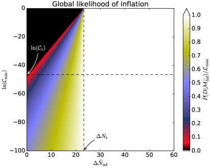
Figure 18: Evidences $p(D|\mathcal{M}_{\mathrm{FL}}^{-})$ for the purely decelerating Friedmann-Lemaître model and $p(D|\mathcal{M}_{\mathrm{inf}}^{-})$ for the inflationary model, given the spatial curvature $\Omega_{\mathcal{K}_{0}}$ measured today (see text). For the FL model, $p(D|\mathcal{M}_{\mathrm{FL}}^{-})$ is obtained for $\Delta\bar{N}_{\mathrm{inf}}=0$ and, hence, corresponds to the vertical axis. The quantity $\mathcal{C}_{\min}$ is the lowest possible value associated with a maximally uninformative prior on the initial absolute relative curvature $\varpi$. The black regions correspond to vanishing evidence for which the model cannot explain the data. In the case of inflation, as soon as $\Delta\bar{N}_{\mathrm{inf}}>\Delta N_{\flat}$, the evidence saturates to $p(D|\mathcal{M}_{\mathrm{inf}}^{-})=\mathcal{L}_{\max}$.

The dependence of $p(D|\mathcal{M}_{\mathrm{inf}}^{-})$ and $p(D|\mathcal{M}_{\mathrm{FL}}^{-})$ with respect to $\mathcal{C}_{\min}$ and $\Delta\bar{N}_{\mathrm{inf}}$ has been plotted in Fig. 18. Black regions in these plots correspond to vanishing evidence and the model cannot explain the current data, i.e., the actual value of $\Omega_{\mathcal{K}_{0}}$. For $\mathcal{M}_{\mathrm{FL}}$, all values of $\mathcal{C}_{\min}$ larger than $\mathcal{C}_{\flat}$, with

$$\ln\mathcal{C}_{\flat}\equiv\ln\left(\dfrac{\sigma_{\pm}}{1\mp\sigma_{\pm}}\right)-N_{0}\simeq-47,$$ (162)

are ruled out. For $\mathcal{M}_{\mathrm{inf}}$, as soon as the number of e-folds $\Delta\bar{N}_{\mathrm{inf}}$ is greater than

$$\Delta N_{\flat}\equiv\dfrac{1}{2}\left[N_{0}-\ln\left(\dfrac{\sigma_{\pm}}{1\mp\sigma_{\pm}}\right)\right]\simeq 24,$$ (163)

the evidence saturates to its maximal value, $\mathcal{L}_{\max}$, independently of $\mathcal{C}_{\min}$. The evidence for the submodel $\mathcal{M}_{\mathrm{inf}}^{+}$ and $\mathcal{M}_{\mathrm{FL}}^{+}$ has not be represented because $\sigma_{\pm}\ll 1$ and they are indistinguishable from the ones plotted in Fig. 18.

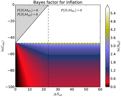
Figure 19: Bayes factor $B_{\mathrm{inf}}\equiv p(D|\mathcal{M}_{\mathrm{inf}})/p(D|\mathcal{M}_{\mathrm{FL}})$ in favor of inflation in the prior parameters plane $(\mathcal{C}_{\min},\Delta\bar{N}_{\mathrm{inf}})$. Up to the small upper-left corner where neither $\mathcal{M}_{\mathrm{FL}}$ nor $\mathcal{M}_{\mathrm{inf}}$ are compatible with the current measurement of curvature, inflation is always favored. In the white region, inflation is compatible with the data whereas $\mathcal{M}_{\mathrm{FL}}$ is not and the Bayes factor for inflation is infinite. For very small values of $\mathcal{C}_{\min}$, $\ln B_{\mathrm{inf}}<1$ and the evidence in favor of inflation becomes “inconclusive” according to the Jeffreys’ scale (see Table 1).

$\ln B_{\mathrm{inf}}$	Odds	Strength of evidence
$<1.0$	$\lesssim 3:1$	Inconclusive
$1.0$	$\sim 3:1$	Weak
$2.5$	$\sim 12:1$	Moderate
$5.0$	$\sim 150:1$	Strong

Table 1: Jeffreys’ scale in the strength of evidence in favor of inflation (from Refs. Gordon and Trotta (2007); Trotta (2008)).

In Fig. 19, we have represented the logarithm of the Bayes factor

$$B_{\mathrm{inf}}^{-}\equiv\dfrac{p(D|\mathcal{M}_{\mathrm{inf}}^{-})}{p(D|\mathcal{M}_{\mathrm{FL}}^{-})}\,,$$ (164)

in favor of inflation. Starting with non-committal model priors, i.e., $\pi(\mathcal{M}_{\mathrm{inf}})=\pi(\mathcal{M}_{\mathrm{FL}})$, $B_{\mathrm{inf}}$ is the factor by how much inflation is more probable than the always decelerating FL model. The correspondence between the values of $B_{\mathrm{inf}}$ and the so-called Jeffreys’ scale is reported in Table 1. As can be checked in Fig. 19, up to the upper-left corner in which both models are ruled out, this factor is always greater than one. In the white region for which $\mathcal{C}_{\min}>\mathcal{C}_{\flat}$, $B_{\mathrm{inf}}^{-}$ is infinite and $\mathcal{M}_{\mathrm{FL}}^{-}$ is ruled out. For $\mathcal{C}_{\min}<\mathcal{C}_{\flat}$, the evidence in favor of inflation rapidly decreases from “strong evidence” around $\mathcal{C}_{\flat}$ to weak and inconclusive evidence around $\mathcal{C}_{\min}=e^{-100}$.

One would obtain almost the same results for the other sign of the curvature and this is why we have not represented the Bayes factor in favor of $\mathcal{M}_{\mathrm{inf}}^{+}$ with respect to $\mathcal{M}_{\mathrm{FL}}^{+}$. Therefore, Fig. 19 is also what one would obtain by adding up the contribution of the two submodels and represents the overall Bayes factor in favor of inflation.

IX.3 Discussion

Let us stress again that the previous results are valid if one only considers the measurement of $\Omega_{\mathcal{K}_{0}}$ today. Some values of $\varpi$ in the previous plots are actually incompatible with many other measurements, such as the age of the universe, the density of matter, …. Moreover, the values for $N_{0}$, $\Delta N_{\flat}$ and $\mathcal{C}_{\flat}$ reported before have been derived under the very conservative hypothesis that $\mathcal{M}_{\mathrm{FL}}$ describes energies lower than $10\,\mathrm{MeV}$ only. If one assumes instead that the FL decelerated evolution starts at higher energies, then $\mathcal{C}_{\flat}$ would be pushed to much lower values while $\Delta N_{\flat}$ would be approaching its fiducial value, around $60$, the value usually reported for inflation to solve the flatness and horizon problems.

Fig. 19 shows that inflation is always a better model hypothesis than a purely decelerating FL model to solve the flatness problem. Both models become equally probable only when one has a theoretical prejudice in which exponentially low values of $\varpi$ within $\mathcal{M}_{\mathrm{FL}}$ are allowed. In particular, taking a flat prior over $\varpi$ effectively consists in taking $\mathcal{C}_{\min}\sim\mathcal{O}\!\left(1\right)$ where $B_{\mathrm{inf}}$ is infinite.

Being agnostic, the prior maximizing ignorance is the one derived in Eq. (150) and requires to specify, at least, one input parameter $\mathcal{C}_{\min}$ (in addition to $\Delta\bar{N}_{\mathrm{inf}}$). The value of $\mathcal{C}_{\min}$ mostly determines the strength of evidence by which inflation is solving the flatness problem compared to standard FL decelerated eras. Let us remark that improving the accuracy by which $\Omega_{\mathcal{K}_{0}}$ is measured, namely reducing the value of $\sigma_{\pm}$, pushes down the value of $\mathcal{C}_{\flat}$. However, this will not change the evidence for inflation if one already has a prior with $\mathcal{C}_{\min}\ll\mathcal{C}_{\flat}$.

In short, if one believes that (or has a theoretical reason why) having an initial curvature smaller than $\varpi_{{\scriptscriptstyle{\mathrm{BBN}}}}=e^{-100}$ is natural within FL cosmology, then the evidence for inflation is indeed “inconclusive”. Otherwise, it seems inevitable.

IX.4 Other instabilities

In the previous section, we have seen that using the prior (or measure) that maximizes ignorance, the Bayesian evidence for inflation to solve the flatness problem still depends on the minimal value allowed for the initial curvature in the decelerating FL model. This one has to be very small, $\varpi_{{\scriptscriptstyle{\mathrm{BBN}}}}<e^{-100}$, to put both models on an equal Bayesian footing.

Various attempts have been made to justify other priors that would render very low values of the initial curvature more probable. As an illustration of this line of reasoning, let us consider again the measure used in Ref. Gibbons and Turok (2008) and given by Eq. (101). Following Ref. Carroll and Tam (2010) and using the fact that $\Omega_{\mathcal{K}}=-\mathcal{K}/(a^{2}H^{2})$, this measure can be rewritten as

$$\omega_{{}_{\scriptscriptstyle{\mathrm{GHS}}},\mathscr{H}=0,H=H_{*}} =-3\sqrt{\frac{3}{2}}\frac{M_{\scriptscriptstyle{\mathrm{Pl}}}}{H_{*}^{2}|\Omega_{\mathcal{K}}|^{5/2}}$$

$$\times\frac{1-\Omega_{V}-2\Omega_{\mathcal{K}}/3}{\sqrt{1-\Omega_{V}-\Omega_{\mathcal{K}}}}\mathrm{d}|\Omega_{\mathcal{K}}|\wedge\mathrm{d}\phi,$$ (165)

in agreement with Eq. (39) of Ref. Carroll and Tam (2010). In the above expression, one has defined $\Omega_{V}\equiv V(\phi)/(3H_{*}^{2}M_{\scriptscriptstyle{\mathrm{Pl}}}^{2})$. This measure has several problems, in particular the fact that it blows up when $\Omega_{\mathcal{K}}\to 0$. In Ref. Carroll and Tam (2010), a scheme of regularization has been proposed which leads to [see their Eq. (56)]

$$\omega_{{}_{\mathrm{GHS}},\mathscr{H}=0,H=H_{*}} \propto\lim\limits_{\epsilon\rightarrow 0}\epsilon^{-3/2}F_{\epsilon}(\Omega_{\mathcal{K}})$$

$$\times\frac{1-\Omega_{V}-2\Omega_{\mathcal{K}}/3}{\sqrt{1-\Omega_{V}-\Omega_{\mathcal{K}}}}\mathrm{d}|\Omega_{\mathcal{K}}|\wedge\mathrm{d}\phi,$$ (166)

where the function $F_{\epsilon}$ tends to a Dirac delta function when $\epsilon$ goes to zero. As a consequence, Ref. Carroll and Tam (2010) obtains

$$\omega_{{\scriptscriptstyle{\mathrm{GHS}}},\mathscr{H}=0,H=H_{*}}\propto\sqrt{1-\Omega_{V}}\delta(\Omega_{\mathcal{K}})\,\mathrm{d}\phi.$$ (167)

Then, Ref. Carroll and Tam (2010) concludes that there is no flatness problem at all. Of course, this argument is based on the use of a regularized GHS measure and, in Sec. VI, we have explained why this is difficult to justify. But the point here is different and the previous considerations simply illustrate that, if one is given a measure strongly peaked at $\Omega_{\mathcal{K}}=0$, then the flatness problem can be alleviated.

Let us, however, stress that, in principle, the curvature parameter cannot be taken arbitrarily small due to the presence of unavoidable quantum or backreaction corrections Bolejko (2017a, b). To understand this point, let us use an analogy with another unstable system, namely a pencil balancing on its tip. If one comes up with a measure in phase-space that is peaked at vanishing tilt angle and initial velocity, it might be tempting to say that the pencil never falls. One might even argue that, in the absence of a well-justified measure, one cannot say whether it is surprising to find a pencil balancing on its tip. In the real world, however, there are always small fluctuations that cause the pencil to fall. Even if one manages to completely suppress thermal fluctuations, because of the Heisenberg uncertainty principle, both the initial angle and velocity cannot be set to zero simultaneously, which causes the pencil to fall in a few seconds Lynch (2014). The same should happen for the curvature parameter, although what value of $\mathcal{C}_{\min}$ quantum fluctuations or cosmological backreaction imply remains to be determined.

X The Multiverse

There exists a last type of criticism that, so far, we have not discussed, although it can play an important role in the literature Ijjas et al. (2013, 2014); Ijjas and Steinhardt (2016) (see also Ref. Guth et al. (2014)). This criticism is related to the claim that inflation necessarily implies the presence of a multiverse that, in turn, would imply a total loss of predictive power.

Inflation might indeed create a multiverse structure when it enters into the regime known as eternal inflation Vilenkin (1983); Linde (1986); Goncharov et al. (1987). Eternal inflation relies on the presence of non-perturbative quantum fluctuations that could affect the background geometry on scales much larger than the Hubble radius. In this picture, our universe could be a small part of an extremely large and inhomogeneous structure, filled with self-reproducing inflationary bubbles. This picture, combined with the effective-field-theory landscape, leads to a multiverse in which the landscape vacua are populated by the eternal inflation mechanism Kachru et al. (2003), and the fundamental constants could vary on the largest length scales.

Let us first notice that, while eternal inflation occurs in some inflationary models, it is not necessarily present in all scenarios, as concretely demonstrated e.g. in Refs. Mukhanov (2015); Dimopoulos and Artymowski (2017). Reference Ijjas and Steinhardt (2016) argues that this type of models is ultra-sensitive to initial conditions. But, according to the considerations in Sec. II, this should not be the case since, even in the presence of corrections, there is no reason not to join the slow-roll attractor solution on the plateau.

Second, the presence of eternal inflation is based on an extrapolation of the inflationary potential very far from the observational window: even if one has established that the potential is, say, a plateau in a regime relevant for cosmology (for which eternal inflation could occur), assuming it remains a plateau everywhere appears to be a strong assumption. If one expects the potential to receive corrections at high energies, then, the question becomes whether these corrections allow the mechanism of eternal inflation to occur, a difficult question since these corrections are usually hard to calculate in detail.

Third, the fact that what we assume at the eternal inflation scale could affect lower energy physics, shows (as it was already discussed for the model building problem) that, to a certain extent, inflation could have UV sensitivities. Although this can be seen as an undesired feature of inflation, let us notice that the standard model of particle physics also has some UV sensitivity (the hierarchy problem for the Higgs mass) but is not discarded for this reason.

Fourth, as explicitly shown in Refs. Ringeval et al. (2010); Hardwick et al. (2017), there are instances where super-Hubble quantum fluctuations actually reinforce inflation’s predictiveness, by washing away dependence on initial conditions that would otherwise be present.

Fifth, in order to properly assess whether the predictive power of inflation is increased or reduced once depicted in the multiverse approach, one needs to justify a measure across the spacetime manifold, and there is no clear procedure for doing that Winitzki (2008); Aguirre et al. (2007); Linde (2007).

Our view is that inflation should be thought of as an effective theory that needs to be tested within its domain of validity only. While the search for connections with higher-energy physics is an interesting and necessary endeavor, the fact that simple extrapolations might cause problems (if they really do) cannot be used as an argument to dismiss the entire model; for the same reason that discarding particle physics on the basis that it is difficult to embed it in an unified framework would appear quite radical.

XI Conclusions

With the advent of high-precision cosmological data, various observational predictions of inflation have been confirmed, which makes it one of the leading paradigms for describing the physics of the very early Universe. However, inflation has also received criticisms, and alternatives (matter bounce Finelli and Brandenberger (2002); Brandenberger (2009); Battefeld and Peter (2015); Brandenberger and Peter (2017), ekpyrotic Khoury et al. (2001, 2002) and cyclic models Steinhardt and Turok (2002), string gas cosmology Brandenberger and Vafa (1989) – as part of emergent universe theories Ellis et al. (2004) –, etc.) have been proposed.

In this article we have reviewed these criticisms and discussed how their status evolved (if it did) with the latest Planck measurements of the CMB temperature and polarization anisotropies. The punchline is that the class of inflationary potentials now favored by the data, namely plateau potentials, is precisely the one for which some of the criticisms raised against inflation are alleviated. This is notably the case for the initial condition problem, at least in an homogeneous situation. We have also shown that this conclusion is robust under UV completions of the models and alternative phase-space measures, and we have underlined the crucial role played by the slow-roll attractor in inflationary dynamics.

Although Planck favors the simplest implementations of inflation, such as Higgs inflation where one does not need to go beyond the Standard Model, or the Starobinsky model where a $R^{2}$ correction is simply added to General Relativity, model building issues remain (such as, for instance, the running of the coupling constants within these scenarios). It would, however, be naive to expect something different given that the energy scale of inflation can be as high as the Grand Unified Theory (GUT) scale. The importance of these issues can be assessed only by gaining more information about Physics at those scales, and they do not constitute inconsistencies of the inflationary mechanism per se.

Concerning the trans-Planckian problem of inflation, the fact that no super-imposed oscillations have been found in the Planck data shows that this effect is small. This confirms that the calculation of the correlation function of inflationary perturbations is robust.

Regarding the multiverse and the criticisms that go with it Ijjas et al. (2014); Ijjas and Steinhardt (2016), it is true that the models singled out by the data are usually associated with a multiverse. But this is the case only if one assumes that the potential remains unchanged way beyond the observational window, which is an additional assumption. In any case, the presence of a multiverse, even in potentials that would allow for it, remains speculative, and does not necessarily imply a loss of predictive power, as we have argued. It seems more reasonable to view inflation as an effective theory that should be used within its domain of validity only. This is similar to the way we use the standard model of particle physics, regardless of what new physics lies beyond it, and despite the fact that this new physics is likely to exist.

There are also criticisms the status of which has not really changed after the Planck data. But we have found that most of these criticisms (likelihood of inflation in the GHS measure, absence of a flatness problem) are not really relevant for inflation. However, questions related to difficulties in the interpretation of Quantum Mechanics remain and affect the discussion about the inflationary mechanism for structure formation.

In our opinion, the major challenge left for inflation is to better determine the conditions under which it can naturally start from highly inhomogeneous initial conditions. This is a difficult and model-dependent question but, clearly, an important issue for having a viable inflationary model.

It is also interesting to notice that the situation is not frozen and that new observations could (and will) change how we view inflation. For instance, the detection of primordial gravitational waves at a level consistent with the simplest models favored by Planck (namely $r\simeq 10^{-3}$) would clearly reinforce our confidence in inflation at high energy. A smoking gun would be the verification of the consistency relation $r=-8n_{\scriptscriptstyle{\mathrm{T}}}$ but, unfortunately, given the present bound on $r$ ($r\lesssim 0.07$), this already appears to be technologically difficult. A measurement of non-Gaussianity would also deeply affect the status of inflation and its preferred implementations.

Inflation appears to be in a better shape after Planck than before, even if, of course, the questions raised by the inflationary theory have not all found fully satisfactory answers.

Appendix A Phase-space volume with the $t$-measure

Let us recall that we consider two vectors ${\bm{u}}_{1}$ and ${\bm{u}}_{2}$ both attached at time $t$ to the point $(\phi,\dot{\phi})$ in phase-space and with components $(\delta\phi_{i},\delta\Pi_{i})$ for $i=1,2$ respectively. They describe an (algebraic) volume given by Eq. (113), namely $\mathscr{V}\left(t\right)={\bm{u}}_{1}\left(t\right)\wedge{\bm{u}}_{2}\left(t\right)=\delta\phi_{1}\delta\Pi_{2}-\delta\Pi_{1}\delta\phi_{2}$. At time $t+\mathrm{d}t$, the point that is located at $(\phi,\Pi)$ at time $t$ moves to

$$\phi \to\phi+\Pi\mathrm{d}t,$$ (168)

$$\Pi \to\Pi+\ddot{\phi}\left(\phi,\Pi\right)\mathrm{d}t.$$

In this expression, $\ddot{\phi}\left(\phi,\Pi\right)$ refers to the equation of motion. In the present case, it is given by Eq. (3). Under this transformation, one obtains

$$\delta\phi_{i} \to\delta\phi_{i}+\delta\Pi_{i}\mathrm{d}t$$ (169)

$$\delta\Pi_{i} \to\delta\Pi_{i}+\frac{\partial\ddot{\phi}\left(\phi,\Pi\right)}{\partial\phi}\delta{\phi}_{i}\mathrm{d}t+\frac{\partial\ddot{\phi}\left(\phi,\Pi\right)}{\partial\Pi}\delta\Pi_{i}\mathrm{d}t.$$ (170)

This gives rise to the coordinates of the vectors ${\bm{u}}_{i}(t+\mathrm{d}t)$ from which one can compute the volume they encompass at time $t+\mathrm{d}t$,

$$\mathscr{V}\left(t+\mathrm{d}t\right) =\left(\delta\phi_{1}\delta\Pi_{2}-\delta\Pi_{1}\delta\phi_{2}\right)\left[1+\frac{\partial\ddot{\phi}\left(\phi,\Pi\right)}{\partial\Pi}\mathrm{d}t+\mathcal{O}\!\left(\mathrm{d}t^{2}\right)\right].$$ (171)

Making use of Eq. (113), one obtains

$$\dfrac{\mathrm{d}\mathscr{V}}{\mathrm{d}t}=\frac{\partial\ddot{\phi}\left(\phi,\Pi\right)}{\partial\Pi}\mathscr{V}\,,$$ (172)

from which one concludes that attractor behaviors correspond to $\partial\ddot{\phi}\left(\phi,\Pi\right)/\partial\Pi<0$. For the field space $t$-measure, Eq. (3) gives rise to

$$\frac{\partial\ddot{\phi}\left(\phi,\Pi\right)}{\partial\Pi}=-3H\left(1+\frac{\Pi^{2}}{6M_{\scriptscriptstyle{\mathrm{Pl}}}^{2}H^{2}}\right).$$ (173)

Combining Eqs. (172) and (173) gives rise to Eq. (114) in the main text.

Appendix B Volume conservation in Hamiltonian measure

Let us now consider a vector ${\bm{u}}_{i}$ in phase-space with components $\delta\phi_{i},\delta p_{\phi,i},\delta a_{i},\delta p_{a,i}$. Because of the motion of the system, this vector changes and, after time $\mathrm{d}t$, the new components are given by

$$\delta\phi_{i} \to\delta\phi_{i}+\dfrac{\partial\dot{\phi}\left(\phi,p_{\phi},a,p_{a}\right)}{\partial\phi}\delta\phi_{i}\mathrm{d}t+\dfrac{\partial\dot{\phi}\left(\phi,p_{\phi},a,p_{a}\right)}{\partial p_{\phi}}\delta p_{\phi,i}\mathrm{d}t+\dfrac{\partial\dot{\phi}\left(\phi,p_{\phi},a,p_{a}\right)}{\partial a}\delta a_{i}\mathrm{d}t+\dfrac{\partial\dot{\phi}\left(\phi,p_{\phi},a,p_{a}\right)}{\partial p_{a}}\delta p_{a,i}\mathrm{d}t,$$ (174)

$$\delta p_{\phi,i} \to\delta p_{\phi,i}+\dfrac{\partial\dot{p_{\phi}}\left(\phi,p_{\phi},a,p_{a}\right)}{\partial\phi}\delta\phi_{i}\mathrm{d}t+\dfrac{\partial\dot{p_{\phi}}\left(\phi,p_{\phi},a,p_{a}\right)}{\partial p_{\phi}}\delta p_{\phi,i}\mathrm{d}t+\dfrac{\partial\dot{p_{\phi}}\left(\phi,p_{\phi},a,p_{a}\right)}{\partial a}\delta a_{i}\mathrm{d}t+\dfrac{\partial\dot{p_{\phi}}\left(\phi,p_{\phi},a,p_{a}\right)}{\partial p_{a}}\delta p_{a,i}\mathrm{d}t,$$ (175)

$$\delta a_{i} \to\delta a_{i}+\dfrac{\partial\dot{a}\left(\phi,p_{\phi},a,p_{a}\right)}{\partial\phi}\delta\phi_{i}\mathrm{d}t+\dfrac{\partial\dot{a}\left(\phi,p_{\phi},a,p_{a}\right)}{\partial p_{\phi}}\delta p_{\phi,i}\mathrm{d}t+\dfrac{\partial\dot{a}\left(\phi,p_{\phi},a,p_{a}\right)}{\partial a}\delta a_{i}\mathrm{d}t+\dfrac{\partial\dot{a}\left(\phi,p_{\phi},a,p_{a}\right)}{\partial p_{a}}\delta p_{a,i}\mathrm{d}t,$$ (176)

$$\delta p_{a,i} \to\delta p_{a,i}+\dfrac{\partial\dot{p_{a}}\left(\phi,p_{\phi},a,p_{a}\right)}{\partial\phi}\delta\phi_{i}\mathrm{d}t+\dfrac{\partial\dot{p_{a}}\left(\phi,p_{\phi},a,p_{a}\right)}{\partial p_{\phi}}\delta p_{\phi,i}\mathrm{d}t+\dfrac{\partial\dot{p_{a}}\left(\phi,p_{\phi},a,p_{a}\right)}{\partial a}\delta a_{i}\mathrm{d}t+\dfrac{\partial\dot{p_{a}}\left(\phi,p_{\phi},a,p_{a}\right)}{\partial p_{a}}\delta p_{a,i}\mathrm{d}t.$$ (177)

As a consequence, the change in the volume generated by four vectors ${\bm{u}}_{1}$, ${\bm{u}}_{2}$, ${\bm{u}}_{3}$ and ${\bm{u}}_{4}$ can be expressed as

$$\mathscr{V}(t)\to\mathscr{V}(t)\left[1+\dfrac{\partial\dot{\phi}\left(\phi,p_{\phi},a,p_{a}\right)}{\partial\phi}+\dfrac{\partial\dot{p_{\phi}}\left(\phi,p_{\phi},a,p_{a}\right)}{\partial p_{\phi}}+\dfrac{\partial\dot{a}\left(\phi,p_{\phi},a,p_{a}\right)}{\partial a}+\dfrac{\partial\dot{p_{a}}\left(\phi,p_{\phi},a,p_{a}\right)}{\partial p_{a}}\right].$$ (178)

We now make use of Hamilton’s equations, namely $\dot{\phi}=\partial\mathscr{H}/\partial p_{\phi}$, $\dot{p}_{\phi}=-\partial\mathscr{H}/\partial\phi$, $\dot{a}=\partial\mathscr{H}/\partial p_{a}$ and $\dot{p}_{a}=-\partial\mathscr{H}/\partial a$ and get

$$\mathscr{V}(t)\to\mathscr{V}(t)\left(1+\dfrac{\partial^{2}\mathscr{H}}{\partial\phi\partial p_{\phi}}-\dfrac{\partial^{2}\mathscr{H}}{\partial p_{\phi}\partial\phi}+\dfrac{\partial^{2}\mathscr{H}}{\partial a\partial p_{a}}-\dfrac{\partial^{2}\mathscr{H}}{\partial p_{a}\partial a}\right)=\mathscr{V}(t).$$ (179)

Therefore, volumes in phase-space are conserved under the Hamiltonian evolution.

Appendix C Phase-space volume with the $N$-measure

For the $N$-measure, the calculation follows in all points the one presented for the $t$-measure in Appendix A. Along the phase-space trajectories, after $\mathrm{d}N$ e-folds of evolution, one has

$$\Phi \to\Phi+\Gamma\mathrm{d}N,$$ (180)

$$\Gamma \to\Gamma+\Gamma_{\negthickspace,N}(\Phi,\Gamma)\,\mathrm{d}N,$$

where $\Gamma_{\negthickspace,N}(\Phi,\Gamma)$ can be read off from Eq. (8) and is given by

$$\Gamma_{\negthickspace,N}(\Phi,\Gamma)\equiv-\left(3-\dfrac{\Gamma^{2}}{2}\right)\left[\Gamma-\Gamma_{\mathrm{sr}}(\Phi)\right].$$ (181)

Similar to Eq. (172), an infinitesimal volume in phase space $(\Phi,\Gamma)$ evolves according to

$$\dfrac{\mathrm{d}\mathscr{V}}{\mathrm{d}N}=\dfrac{\partial\Gamma_{\negthickspace,N}(\Phi,\Gamma)}{\partial\Gamma}\mathscr{V}=\left[-3\left(1-\dfrac{1}{2}\Gamma^{2}\right)-\Gamma\Gamma_{\mathrm{sr}}(\Phi)\right]\mathscr{V}.$$ (182)

Introducing

$$\Gamma_{\pm}(\Phi)=\pm\sqrt{2+\dfrac{\Gamma_{\mathrm{sr}}^{2}(\Phi)}{9}}+\dfrac{\Gamma_{\mathrm{sr}}(\Phi)}{3}\,,$$ (183)

this gives rise to Eq. (117) in the main text.

Appendix D Flow compression with the $t$-measure

Let us consider a point $M_{0}$ in phase-space of coordinates $M_{0}(\phi_{0},\dot{\phi}_{0})$ at time $t$. In the neighborhood of $M_{0}$, its orbit is parametrized by

$$\mathscr{C}\left(M_{0}\right)\simeq\left\{\left[\phi_{0}+\dot{\phi}_{0}u,\dot{\phi}_{0}+\ddot{\phi}\left(\phi_{0},\dot{\phi}_{0}\right)u\right],u\in\mathbb{R}\right\},$$ (184)

where $u$ is a dummy parameter and, as explained in Appendix A, $\ddot{\phi}\left(\phi,\dot{\phi}\right)$ is given by Eq. (3). At time $t+\mathrm{d}t$, this point becomes $M_{1}$ with coordinates $M_{1}[\phi_{0}+\dot{\phi}_{0}\mathrm{d}t,\dot{\phi}_{0}+\ddot{\phi}\left(\phi_{0},\dot{\phi}_{0}\right)\mathrm{d}t]$ which obviously belongs to $\mathscr{C}(M_{0})$. We now consider another point $N_{0}$ infinitesimally displaced away from $M_{0}$, $N_{0}(\phi_{0}+\delta\phi,\dot{\phi}_{0}+\delta\dot{\phi})$, at time $t$. In the neighborhood of $N_{0}$ (and of $M_{0}$), its orbit is given by

$$\mathscr{C}\left(N_{0}\right)\simeq \left\{\left[\phi_{0}+\delta\phi+\left(\dot{\phi}_{0}+\delta\dot{\phi}\right)u,\dot{\phi}_{0}+\delta\dot{\phi}+\ddot{\phi}\left(\phi_{0}+\delta\phi,\dot{\phi}_{0}+\delta\dot{\phi}\right)u\right],u\in\mathbb{R}\right\}\,.$$ (185)

At time $t+\mathrm{d}t$, this point becomes $N_{1}$ with coordinates

$$N_{1}[ \phi_{0}+\delta\phi+\left(\dot{\phi}_{0}+\delta\dot{\phi}\right)\mathrm{d}t,\dot{\phi}_{0}+\delta\dot{\phi}+\ddot{\phi}\left(\phi_{0}+\delta\phi,\dot{\phi}_{0}+\delta\dot{\phi}\right)\mathrm{d}t],$$ (186)

which obviously belongs to $\mathscr{C}(N_{0})$. Let us now calculate how the distance $\mathscr{D}$ between these two points evolves between times $t$ and $t+\mathrm{d}t$.

Let us consider a point $N$ belonging to $\mathscr{C}(N_{0})$ with parameter $u$. The distance between $M_{0}$ and $N$ is given by

$$d^{2}\left(M_{0},N\right)=\mu^{2}\left[\delta\phi+\left(\dot{\phi}_{0}+\delta\dot{\phi}\right)u\right]^{2}+\left[\delta\dot{\phi}+\ddot{\phi}\left(\phi_{0}+\delta\phi,\dot{\phi}_{0}+\delta\dot{\phi}\right)u\right]^{2}.$$ (187)

By minimizing the above quantity over $u$, one finds

$$d^{2}\left[M_{0},\mathscr{C}\left(N_{0}\right)\right]=\dfrac{\mu^{2}\left[\delta\dot{\phi}\left(\dot{\phi}_{0}+\delta\dot{\phi}\right)-\delta\phi\ddot{\phi}\left(\phi_{0}+\delta\phi,\dot{\phi}_{0}+\delta\dot{\phi}\right)\right]^{2}}{\mu^{2}\left(\dot{\phi}_{0}+\delta\dot{\phi}\right)^{2}+\ddot{\phi}^{2}\left(\phi_{0}+\delta\phi,\dot{\phi}_{0}+\delta\dot{\phi}\right)}\,.$$ (188)

In the same manner, one can consider a point $M$ belonging to $\mathscr{C}(M_{0})$ with parameter $u$. The distance between $N_{0}$ and $M$ is given by

$$d^{2}\left(N_{0},M\right)=\mu^{2}\left(\delta\phi-\dot{\phi}_{0}u\right)^{2}+\left[\delta\dot{\phi}-\ddot{\phi}\left(\phi_{0},\dot{\phi}_{0}\right)u\right]^{2}\,.$$ (189)

By minimizing this quantity over $u$, one finds

$$d^{2}\left[N_{0},\mathscr{C}\left(M_{0}\right)\right]=\dfrac{\mu^{2}\left[\dot{\phi}_{0}\delta\dot{\phi}-\delta\phi\ddot{\phi}\left(\phi_{0},\dot{\phi}_{0}\right)\right]^{2}}{\mu^{2}\dot{\phi}_{0}^{2}+\ddot{\phi}^{2}\left(\phi_{0},\dot{\phi}_{0}\right)}\,.$$ (190)

Let us now consider again a point $N$ belonging to $\mathscr{C}(N_{1})=\mathscr{C}(N_{0})$ with parameter $u$. The distance between $M_{1}$ and $N$ is given by

$$d^{2}\left(M_{1},N\right)=\mu^{2}\left[\delta\phi+\left(\dot{\phi}_{0}+\delta\dot{\phi}\right)u-\dot{\phi}_{0}\mathrm{d}t\right]^{2}+\left[\delta\dot{\phi}+\ddot{\phi}\left(\phi_{0}+\delta\phi,\dot{\phi}_{0}+\delta\dot{\phi}\right)u-\ddot{\phi}\left(\phi_{0},\dot{\phi}_{0}\right)\mathrm{d}t\right]^{2}.$$ (191)

By minimizing this quantity over $u$, one finds

$$d^{2}\left[M_{1},\mathscr{C}\left(N_{1}\right)\right]=\dfrac{\mu^{2}\left\{\left(\dot{\phi}_{0}+\delta\dot{\phi}\right)\left[\delta\dot{\phi}-\ddot{\phi}\left(\phi_{0},\dot{\phi}_{0}\right)\mathrm{d}t\right]-\left(\delta\phi-\dot{\phi}_{0}\mathrm{d}t\right)\ddot{\phi}\left(\phi_{0}+\delta\phi,\dot{\phi}_{0}+\delta\dot{\phi}\right)\right\}^{2}}{\mu^{2}\left(\dot{\phi}_{0}+\delta\dot{\phi}\right)^{2}+\ddot{\phi}^{2}\left(\phi_{0}+\delta\phi,\dot{\phi}_{0}+\delta\dot{\phi}\right)}\,.$$ (192)

In the same manner, considering a point $M$ belonging to $\mathscr{C}(M_{1})=\mathscr{C}(M_{0})$ with parameter $u$, the distance between $N_{1}$ and $M$ is given by

$$d^{2}\left(N_{1},M\right)=\mu^{2}\left[\delta\phi+\left(\dot{\phi}_{0}+\delta\dot{\phi}\right)\mathrm{d}t-\dot{\phi}_{0}u\right]^{2}+\left[\delta\dot{\phi}+\ddot{\phi}\left(\phi_{0}+\delta\phi,\dot{\phi}_{0}+\delta\dot{\phi}\right)\mathrm{d}t-\ddot{\phi}\left(\phi_{0},\dot{\phi}_{0}\right)u\right]^{2}\,.$$ (193)

By minimizing this quantity over $u$, one finds

$$d^{2}\left[N_{1},\mathscr{C}\left(M_{1}\right)\right]=\dfrac{\mu^{2}\left\{\dot{\phi}_{0}\left[\delta\dot{\phi}+\ddot{\phi}\left(\phi_{0}+\delta\phi,\dot{\phi}_{0}+\delta\dot{\phi}\right)\mathrm{d}t\right]-\left[\delta\phi+\left(\dot{\phi}_{0}+\delta\dot{\phi}\right)\mathrm{d}t\right]\ddot{\phi}\left(\phi_{0},\dot{\phi}_{0}\right)\right\}^{2}}{\mu^{2}\dot{\phi}_{0}^{2}+\ddot{\phi}^{2}\left(\phi_{0},\dot{\phi}_{0}\right)}\,.$$ (194)

Expanding the previous expressions at quadratic order in $\delta\phi$ and $\delta\dot{\phi}$, and at leading order in $\mathrm{d}t$, one obtains

$$d^{2}\left[M_{0},\mathscr{C}\left(N_{0}\right)\right] =d^{2}\left[N_{0},\mathscr{C}\left(M_{0}\right)\right]=\dfrac{\mu^{2}\left(\dot{\phi}_{0}\delta\dot{\phi}-\delta\phi\ddot{\phi}_{0}\right)^{2}}{\mu^{2}\dot{\phi}_{0}^{2}+\ddot{\phi}_{0}^{2}}\,,$$ (195)

$$d^{2}\left[M_{1},\mathscr{C}\left(N_{1}\right)\right] =d^{2}\left[N_{1},\mathscr{C}\left(M_{1}\right)\right]=\dfrac{\mu^{2}\left(\dot{\phi}_{0}\delta\dot{\phi}-\delta\phi\ddot{\phi}_{0}\right)^{2}}{\mu^{2}\dot{\phi}_{0}^{2}+\ddot{\phi}_{0}^{2}}+2\mathrm{d}t\dfrac{\mu^{2}\left(\dot{\phi}_{0}\delta\dot{\phi}-\delta\phi\ddot{\phi}_{0}\right)}{\mu^{2}\dot{\phi}_{0}^{2}+\ddot{\phi}_{0}^{2}}\left(\dot{\phi}_{0}\dfrac{\partial\ddot{\phi}}{\partial\phi}\delta\phi+\dfrac{\partial\ddot{\phi}}{\partial\dot{\phi}}\dot{\phi}_{0}\delta\dot{\phi}-\ddot{\phi}_{0}\delta\dot{\phi}\right)\,,$$ (196)

where we have defined $\ddot{\phi}_{0}\equiv\ddot{\phi}\left(\phi_{0},\dot{\phi}_{0}\right)$. It is interesting to notice that at leading order, $d^{2}[M_{0},\mathscr{C}(N_{0})]=d^{2}[N_{0},\mathscr{C}(M_{0})]$ and $d^{2}[M_{1},\mathscr{C}(N_{1})]=d^{2}[N_{1},\mathscr{C}(M_{1})]$. This implies that in the definition (119), any way to symmetrize the expression would give the same result below. The above expression gives rise to

$$\dfrac{\mathrm{d}\mathscr{D}^{2}}{\mathrm{d}t}=2\dfrac{\mu^{2}\left(\dot{\phi}_{0}\delta\dot{\phi}-\delta\phi\ddot{\phi}_{0}\right)}{\mu^{2}\dot{\phi}_{0}^{2}+\ddot{\phi}_{0}^{2}}\left(\dot{\phi}_{0}\dfrac{\partial\ddot{\phi}}{\partial\phi}\delta\phi+\dfrac{\partial\ddot{\phi}}{\partial\dot{\phi}}\dot{\phi}_{0}\delta\dot{\phi}-\ddot{\phi}_{0}\delta\dot{\phi}\right),$$ (197)

and one obtains

$$\dfrac{\mathrm{d}\ln\mathscr{D}}{\mathrm{d}t}=\dfrac{\dot{\phi}_{0}\dfrac{\partial\ddot{\phi}}{\partial\phi}\delta\phi+\dfrac{\partial\ddot{\phi}}{\partial\dot{\phi}}\dot{\phi}_{0}\delta\dot{\phi}-\ddot{\phi}_{0}\delta\dot{\phi}}{\dot{\phi}_{0}\delta\dot{\phi}-\delta\phi\ddot{\phi}_{0}}\,.$$ (198)

Making use of Eq. (3) to evaluate the function $\ddot{\phi}(\phi,\dot{\phi})$, this gives rise to Eq. (121) in the main text.

Appendix E Flow compression with the Hamiltonian induced measure

As explained in Sec. VII.1.3, in order to be explicitly defined, the Hamiltonian induced measure needs to come with a choice of hypersurfaces of constant time in phase-space. Here, this choice is given by the scale $\mu$, in such a way that distances computed at a given time $t$ are measured along phase-space directions where the scale factor is constant and equal to $a(t)$, such that $d^{2}=\mu^{2}\delta\phi^{2}+a^{6}(t)\delta\dot{\phi}^{2}$.

The calculation then proceeds in a way that is very similar to Appendix D. For instance, Eq. (187) needs to be replaced with

$$d^{2}\left(M_{0},N\right)=\mu^{2}\left[\delta\phi+\left(\dot{\phi}_{0}+\delta\dot{\phi}\right)u\right]^{2}+a^{6}(t)\left[\delta\dot{\phi}+\ddot{\phi}\left(\phi_{0}+\delta\phi,\dot{\phi}_{0}+\delta\dot{\phi}\right)u\right]^{2},$$ (199)

which gives rise to

$$d^{2}\left[M_{0},\mathscr{C}\left(N_{0}\right)\right]=\dfrac{\mu^{2}a^{6}(t)\left[\delta\dot{\phi}\left(\dot{\phi}_{0}+\delta\dot{\phi}\right)-\delta\phi\ddot{\phi}\left(\phi_{0}+\delta\phi,\dot{\phi}_{0}+\delta\dot{\phi}\right)\right]^{2}}{\mu^{2}\left(\dot{\phi}_{0}+\delta\dot{\phi}\right)^{2}+a^{6}(t)\ddot{\phi}^{2}\left(\phi_{0}+\delta\phi,\dot{\phi}_{0}+\delta\dot{\phi}\right)}$$ (200)

instead of Eq. (188). The same modifications apply to Eqs. (189) and (190), as well as to Eqs. (191)-(194) except that the scale factor needs to be evaluated at time $t+\mathrm{d}t$ in the latter set of equations. Instead of Eqs. (195) and (196), one then has

$$d^{2}\left[M_{0},\mathscr{C}\left(N_{0}\right)\right] =d^{2}\left[N_{0},\mathscr{C}\left(M_{0}\right)\right]=\dfrac{\mu^{2}a^{6}(t)\left(\dot{\phi}_{0}\delta\dot{\phi}-\delta\phi\ddot{\phi}_{0}\right)^{2}}{\mu^{2}\dot{\phi}_{0}^{2}+a^{6}(t)\ddot{\phi}_{0}^{2}}\,,$$ (201)

$$d^{2}\left[M_{1},\mathscr{C}\left(N_{1}\right)\right] =d^{2}\left[N_{1},\mathscr{C}\left(M_{1}\right)\right]=\dfrac{\mu^{2}a^{6}(t+\mathrm{d}t)\left[\dot{\phi}_{0}\delta\dot{\phi}-\delta\phi\ddot{\phi}_{0}+\dot{\phi}_{0}\dfrac{\partial\ddot{\phi}}{\partial\phi}\delta\phi\mathrm{d}t+\left(\dfrac{\partial\ddot{\phi}}{\partial\dot{\phi}}\dot{\phi}_{0}-\ddot{\phi}_{0}\right)\delta\dot{\phi}\mathrm{d}t\right]^{2}}{\mu^{2}\dot{\phi}_{0}^{2}+a^{6}(t+\mathrm{d}t)\ddot{\phi}^{2}_{0}}+\mathcal{O}\!\left[\left(\delta\phi,\delta\dot{\phi}\right)^{3}\right].$$ (202)

One then obtains an additional term compared to the $t$-measure, that does not depend on $\delta\phi$ and $\delta\dot{\phi}$, namely

$$\dfrac{\mathrm{d}\ln\mathscr{D}}{\mathrm{d}t}=\dfrac{\dot{\phi}_{0}\dfrac{\partial\ddot{\phi}}{\partial\phi}\delta\phi+\dfrac{\partial\ddot{\phi}}{\partial\dot{\phi}}\dot{\phi}_{0}\delta\dot{\phi}-\ddot{\phi}_{0}\delta\dot{\phi}}{\dot{\phi}_{0}\delta\dot{\phi}-\delta\phi\ddot{\phi}_{0}}+3\dfrac{\mu^{2}H\dot{\phi}_{0}^{2}}{\mu^{2}\dot{\phi}_{0}^{2}+\ddot{\phi}_{0}^{2}}\,.$$ (203)

In terms of the slow-roll functions, this gives rise to Eq. (125) in the main text.

References

- Starobinsky (1979) A. A. Starobinsky, JETP Lett. 30, 682 (1979).
- Starobinsky (1980) A. A. Starobinsky, Phys. Lett. B91, 99 (1980).
- Guth (1981) A. H. Guth, Phys. Rev. D23, 347 (1981).
- Linde (1982) A. D. Linde, Phys. Lett. B108, 389 (1982).
- Albrecht and Steinhardt (1982) A. Albrecht and P. J. Steinhardt, Phys. Rev. Lett. 48, 1220 (1982).
- Linde (1983) A. D. Linde, Phys. Lett. B129, 177 (1983).
- Mukhanov and Chibisov (1981) V. F. Mukhanov and G. V. Chibisov, JETP Lett. 33, 532 (1981), [Pisma Zh. Eksp. Teor. Fiz.33,549(1981)].
- Mukhanov and Chibisov (1982) V. F. Mukhanov and G. V. Chibisov, Sov. Phys. JETP 56, 258 (1982), [Zh. Eksp. Teor. Fiz.83,475(1982)].
- Starobinsky (1982) A. A. Starobinsky, Phys. Lett. B117, 175 (1982).
- Guth and Pi (1982) A. H. Guth and S. Y. Pi, Phys. Rev. Lett. 49, 1110 (1982).
- Hawking (1982) S. W. Hawking, Phys. Lett. B115, 295 (1982).
- Bardeen et al. (1983) J. M. Bardeen, P. J. Steinhardt, and M. S. Turner, Phys. Rev. D28, 679 (1983).
- Guth et al. (2014) A. H. Guth, D. I. Kaiser, and Y. Nomura, Phys. Lett. B733, 112 (2014), eprint 1312.7619.
- Linde (2015) A. Linde, in Proceedings, 100th Les Houches Summer School: Post-Planck Cosmology: Les Houches, France, July 8 - August 2, 2013 (2015), pp. 231–316, eprint 1402.0526.
- Mishra et al. (2018) S. S. Mishra, V. Sahni, and A. V. Toporensky, Phys. Rev. D98, 083538 (2018), eprint 1801.04948.
- Marsh et al. (2018) M. C. D. Marsh, J. D. Barrow, and C. Ganguly, JCAP 1805, 026 (2018), eprint 1803.00625.
- Ijjas et al. (2013) A. Ijjas, P. J. Steinhardt, and A. Loeb, Phys. Lett. B723, 261 (2013), eprint 1304.2785.
- Goldwirth and Piran (1990) D. S. Goldwirth and T. Piran, Phys. Rev. Lett. 64, 2852 (1990).
- Goldwirth and Piran (1992) D. S. Goldwirth and T. Piran, Phys. Rept. 214, 223 (1992).
- Schwarz et al. (2001) D. J. Schwarz, C. A. Terrero-Escalante, and A. A. Garcia, Phys. Lett. B517, 243 (2001), eprint astro-ph/0106020.
- Schwarz and Terrero-Escalante (2004) D. J. Schwarz and C. A. Terrero-Escalante, JCAP 0408, 003 (2004), eprint hep-ph/0403129.
- Kinney (2005) W. H. Kinney, Phys. Rev. D72, 023515 (2005), eprint gr-qc/0503017.
- Martin et al. (2013) J. Martin, H. Motohashi, and T. Suyama, Phys. Rev. D87, 023514 (2013), eprint 1211.0083.
- Motohashi et al. (2015) H. Motohashi, A. A. Starobinsky, and J. Yokoyama, JCAP 1509, 018 (2015), eprint 1411.5021.
- Linde (2001) A. D. Linde, JHEP 11, 052 (2001), eprint hep-th/0110195.
- Handley et al. (2014) W. J. Handley, S. D. Brechet, A. N. Lasenby, and M. P. Hobson, Phys. Rev. D89, 063505 (2014), eprint 1401.2253.
- Pattison et al. (2018) C. Pattison, V. Vennin, H. Assadullahi, and D. Wands, JCAP 1808, 048 (2018), eprint 1806.09553.
- Ringeval (2008) C. Ringeval, Lect. Notes Phys. 738, 243 (2008), eprint astro-ph/0703486.
- Ringeval (2014) C. Ringeval, Mon. Not. Roy. Astron. Soc. 439, 3253 (2014), eprint 1312.2347.
- Martin et al. (2014a) J. Martin, C. Ringeval, and V. Vennin, Phys. Dark Univ. 5-6, 75 (2014a), eprint 1303.3787.
- Boubekeur and Lyth (2005) L. Boubekeur and D. H. Lyth, JCAP 0507, 010 (2005), eprint hep-ph/0502047.
- Tzirakis and Kinney (2007) K. Tzirakis and W. H. Kinney, Phys. Rev. D75, 123510 (2007), eprint astro-ph/0701432.
- Enckell et al. (2018) V.-M. Enckell, K. Enqvist, S. Rasanen, and E. Tomberg, JCAP 1806, 005 (2018), eprint 1802.09299.
- Martin et al. (2014b) J. Martin, C. Ringeval, R. Trotta, and V. Vennin, JCAP 1403, 039 (2014b), eprint 1312.3529.
- Yokoyama (1998) J. Yokoyama, Phys. Rev. D58, 083510 (1998), eprint astro-ph/9802357.
- Kallosh and Linde (2013) R. Kallosh and A. Linde, JCAP 1307, 002 (2013), eprint 1306.5220.
- Artymowski et al. (2015) M. Artymowski, Z. Lalak, and M. Lewicki, JCAP 1506, 032 (2015), eprint 1502.01371.
- Artymowski et al. (2016) M. Artymowski, Z. Lalak, and M. Lewicki, Phys. Rev. D93, 043514 (2016), eprint 1509.00031.
- De Felice and Tsujikawa (2010) A. De Felice and S. Tsujikawa, Living Rev. Rel. 13, 3 (2010), eprint 1002.4928.
- Bezrukov and Shaposhnikov (2008) F. Bezrukov and M. Shaposhnikov, Phys.Lett. B659, 703 (2008), eprint 0710.3755.
- Barvinsky et al. (2008) A. O. Barvinsky, A. Yu. Kamenshchik, and A. A. Starobinsky, JCAP 0811, 021 (2008), eprint 0809.2104.
- De Simone et al. (2009) A. De Simone, M. P. Hertzberg, and F. Wilczek, Phys. Lett. B678, 1 (2009), eprint 0812.4946.
- Bezrukov et al. (2011) F. Bezrukov, A. Magnin, M. Shaposhnikov, and S. Sibiryakov, JHEP 01, 016 (2011), eprint 1008.5157.
- Kunz et al. (2006) M. Kunz, R. Trotta, and D. Parkinson, Phys. Rev. D74, 023503 (2006), eprint astro-ph/0602378.
- Lewis (2013) A. Lewis, Phys. Rev. D87, 103529 (2013), eprint 1304.4473.
- Steigman and Turner (1983) G. Steigman and M. S. Turner, Phys. Lett. 128B, 295 (1983).
- Anninos et al. (1991) P. Anninos, R. A. Matzner, T. Rothman, and M. P. Ryan, Phys. Rev. D43, 3821 (1991).
- Turner and Widrow (1986) M. S. Turner and L. M. Widrow, Phys. Rev. Lett. 57, 2237 (1986).
- Albrecht and Brandenberger (1985) A. Albrecht and R. H. Brandenberger, Phys. Rev. D31, 1225 (1985).
- Albrecht et al. (1985) A. Albrecht, R. H. Brandenberger, and R. Matzner, Phys. Rev. D32, 1280 (1985).
- Albrecht et al. (1987) A. Albrecht, R. H. Brandenberger, and R. Matzner, Phys. Rev. D35, 429 (1987).
- Brandenberger (2016) R. Brandenberger, Int. J. Mod. Phys. D26, 1740002 (2016), eprint 1601.01918.
- Vachaspati and Trodden (1999) T. Vachaspati and M. Trodden, Phys. Rev. D61, 023502 (1999), eprint gr-qc/9811037.
- Berera and Gordon (2001) A. Berera and C. Gordon, Phys. Rev. D63, 063505 (2001), eprint hep-ph/0010280.
- Easther et al. (2014) R. Easther, L. C. Price, and J. Rasero, JCAP 1408, 041 (2014), eprint 1406.2869.
- Goldwirth and Piran (1989) D. S. Goldwirth and T. Piran, Phys. Rev. D40, 3263 (1989).
- Goldwirth (1991) D. S. Goldwirth, Phys. Rev. D43, 3204 (1991).
- Kurki-Suonio et al. (1987) H. Kurki-Suonio, R. A. Matzner, J. Centrella, and J. R. Wilson, Phys. Rev. D35, 435 (1987).
- Laguna et al. (1991) P. Laguna, H. Kurki-Suonio, and R. A. Matzner, Phys. Rev. D44, 3077 (1991).
- Kurki-Suonio et al. (1993) H. Kurki-Suonio, P. Laguna, and R. A. Matzner, Phys. Rev. D48, 3611 (1993), eprint astro-ph/9306009.
- East et al. (2016) W. E. East, M. Kleban, A. Linde, and L. Senatore, JCAP 1609, 010 (2016), eprint 1511.05143.
- Clough et al. (2017) K. Clough, E. A. Lim, B. S. DiNunno, W. Fischler, R. Flauger, and S. Paban, JCAP 1709, 025 (2017), eprint 1608.04408.
- Bloomfield et al. (2019) J. K. Bloomfield, P. Fitzpatrick, K. Hilbert, and D. I. Kaiser, Phys. Rev. D100, 063512 (2019), eprint 1906.08651.
- Calzetta and Sakellariadou (1992) E. Calzetta and M. Sakellariadou, Phys. Rev. D45, 2802 (1992).
- Perez and Pinto-Neto (2011) R. S. Perez and N. Pinto-Neto, Grav. Cosmol. 17, 136 (2011), eprint 1205.3790.
- Linde (1984) A. D. Linde, Sov. Phys. JETP 60, 211 (1984), [Zh. Eksp. Teor. Fiz.87,369(1984)].
- Linde (1985) A. D. Linde, Phys. Lett. 162B, 281 (1985).
- Coule and Martin (2000) D. H. Coule and J. Martin, Phys. Rev. D61, 063501 (2000), eprint gr-qc/9905056.
- Martin and Brandenberger (2001) J. Martin and R. H. Brandenberger, Phys. Rev. D63, 123501 (2001), eprint hep-th/0005209.
- Brandenberger and Martin (2001) R. H. Brandenberger and J. Martin, Mod. Phys. Lett. A16, 999 (2001), eprint astro-ph/0005432.
- Brandenberger and Martin (2013) R. H. Brandenberger and J. Martin, Class. Quant. Grav. 30, 113001 (2013), eprint 1211.6753.
- Brandenberger and Martin (2005) R. H. Brandenberger and J. Martin, Phys. Rev. D71, 023504 (2005), eprint hep-th/0410223.
- Martin and Brandenberger (2003) J. Martin and R. Brandenberger, Phys. Rev. D68, 063513 (2003), eprint hep-th/0305161.
- Martin and Brandenberger (2002) J. Martin and R. H. Brandenberger, Phys. Rev. D65, 103514 (2002), eprint hep-th/0201189.
- Brandenberger and Martin (2002) R. H. Brandenberger and J. Martin, Int. J. Mod. Phys. A17, 3663 (2002), eprint hep-th/0202142.
- Martin and Ringeval (2004a) J. Martin and C. Ringeval, Phys. Rev. D69, 083515 (2004a), eprint astro-ph/0310382.
- Martin and Ringeval (2005) J. Martin and C. Ringeval, JCAP 0501, 007 (2005), eprint hep-ph/0405249.
- Martin and Ringeval (2004b) J. Martin and C. Ringeval, Phys. Rev. D69, 127303 (2004b), eprint astro-ph/0402609.
- Martin and Ringeval (2006) J. Martin and C. Ringeval, JCAP 0608, 009 (2006), eprint astro-ph/0605367.
- Martin and Brandenberger (2000) J. Martin and R. H. Brandenberger, in Recent developments in theoretical and experimental general relativity, gravitation and relativistic field theories. Proceedings, 9th Marcel Grossmann Meeting, MG’9, Rome, Italy, July 2-8, 2000. Pts. A-C (2000), pp. 2001–2002, eprint astro-ph/0012031.
- Easther et al. (2001) R. Easther, B. R. Greene, W. H. Kinney, and G. Shiu, Phys. Rev. D64, 103502 (2001), eprint hep-th/0104102.
- Easther et al. (2002) R. Easther, B. R. Greene, W. H. Kinney, and G. Shiu, Phys. Rev. D66, 023518 (2002), eprint hep-th/0204129.
- Armendariz-Picon and Lim (2003) C. Armendariz-Picon and E. A. Lim, JCAP 0312, 006 (2003), eprint hep-th/0303103.
- Easther et al. (2005) R. Easther, W. H. Kinney, and H. Peiris, JCAP 0505, 009 (2005), eprint astro-ph/0412613.
- Polarski and Starobinsky (1996) D. Polarski and A. A. Starobinsky, Class. Quant. Grav. 13, 377 (1996), eprint gr-qc/9504030.
- Kiefer et al. (1998) C. Kiefer, D. Polarski, and A. A. Starobinsky, Int. J. Mod. Phys. D7, 455 (1998), eprint gr-qc/9802003.
- Martin and Vennin (2016a) J. Martin and V. Vennin, Phys. Rev. D93, 023505 (2016a), eprint 1510.04038.
- Martin and Vennin (2016b) J. Martin and V. Vennin, Phys. Rev. A93, 062117 (2016b), eprint 1605.02944.
- Martin and Vennin (2017) J. Martin and V. Vennin, Phys. Rev. D96, 063501 (2017), eprint 1706.05001.
- Sudarsky (2011) D. Sudarsky, Int. J. Mod. Phys. D20, 509 (2011), eprint 0906.0315.
- Goldstein et al. (2015) S. Goldstein, W. Struyve, and R. Tumulka (2015), eprint 1508.01017.
- Hartle et al. (2019) J. B. Hartle, U. o. California, and S. Barbara (2019), eprint 1901.03933.
- Kiefer et al. (2007) C. Kiefer, I. Lohmar, D. Polarski, and A. A. Starobinsky, Class. Quant. Grav. 24, 1699 (2007), eprint astro-ph/0610700.
- Perez et al. (2006) A. Perez, H. Sahlmann, and D. Sudarsky, Class. Quant. Grav. 23, 2317 (2006), eprint gr-qc/0508100.
- De Unanue and Sudarsky (2008) A. De Unanue and D. Sudarsky, Phys. Rev. D78, 043510 (2008), eprint 0801.4702.
- Leon and Sudarsky (2010) G. Leon and D. Sudarsky, Class. Quant. Grav. 27, 225017 (2010), eprint 1003.5950.
- Martin et al. (2012) J. Martin, V. Vennin, and P. Peter, Phys. Rev. D86, 103524 (2012), eprint 1207.2086.
- Cañate et al. (2013) P. Cañate, P. Pearle, and D. Sudarsky, Phys. Rev. D87, 104024 (2013), eprint 1211.3463.
- Das et al. (2013) S. Das, K. Lochan, S. Sahu, and T. P. Singh, Phys. Rev. D88, 085020 (2013), [Erratum: Phys. Rev.D89,no.10,109902(2014)], eprint 1304.5094.
- Peter et al. (2007) P. Peter, E. J. C. Pinho, and N. Pinto-Neto, Phys. Rev. D75, 023516 (2007), eprint hep-th/0610205.
- Pinto-Neto et al. (2012) N. Pinto-Neto, G. Santos, and W. Struyve, Phys. Rev. D85, 083506 (2012), eprint 1110.1339.
- Peter and Vitenti (2016) P. Peter and S. D. P. Vitenti, Mod. Phys. Lett. A31, 1640006 (2016), eprint 1603.02342.
- Gibbons et al. (1987) G. W. Gibbons, S. W. Hawking, and J. M. Stewart, Nucl. Phys. B281, 736 (1987).
- Schiffrin and Wald (2012) J. S. Schiffrin and R. M. Wald, Phys. Rev. D86, 023521 (2012), eprint 1202.1818.
- Gibbons and Turok (2008) G. W. Gibbons and N. Turok, Phys. Rev. D77, 063516 (2008), eprint hep-th/0609095.
- Corichi and Sloan (2014) A. Corichi and D. Sloan, Class. Quant. Grav. 31, 062001 (2014), eprint 1310.6399.
- Carroll and Tam (2010) S. M. Carroll and H. Tam (2010), eprint 1007.1417.
- Ijjas and Steinhardt (2016) A. Ijjas and P. J. Steinhardt, Class. Quant. Grav. 33, 044001 (2016), eprint 1512.09010.
- Finn and Karamitsos (2019) K. Finn and S. Karamitsos, Phys. Rev. D99, 063515 (2019), [Erratum: Phys. Rev.D99,no.10,109901(2019)], eprint 1812.07095.
- Remmen and Carroll (2013) G. N. Remmen and S. M. Carroll, Phys. Rev. D88, 083518 (2013), eprint 1309.2611.
- J. (1941) D. J., Transactions of the American Mathematical Society 50(1), 71 (1941).
- Clesse et al. (2009) S. Clesse, C. Ringeval, and J. Rocher, Phys. Rev. D80, 123534 (2009), eprint 0909.0402.
- Vennin (2014) V. Vennin, Phys. Rev. D89, 083526 (2014), eprint 1401.2926.
- Liddle et al. (1994) A. R. Liddle, P. Parsons, and J. D. Barrow, Phys. Rev. D50, 7222 (1994), eprint astro-ph/9408015.
- Golovnev et al. (2008) A. Golovnev, V. Mukhanov, and V. Vanchurin, JCAP 0806, 009 (2008), eprint 0802.2068.
- Aad et al. (2012) G. Aad et al. (ATLAS), Phys. Lett. B716, 1 (2012), eprint 1207.7214.
- Baumann and McAllister (2015) D. Baumann and L. McAllister, Inflation and String Theory (Cambridge University Press, 2015), ISBN 9781107089693, 9781316237182, eprint 1404.2601.
- Kawasaki et al. (2000) M. Kawasaki, M. Yamaguchi, and T. Yanagida, Phys. Rev. Lett. 85, 3572 (2000), eprint hep-ph/0004243.
- Cai et al. (2015) Y.-F. Cai, J.-O. Gong, S. Pi, E. N. Saridakis, and S.-Y. Wu, Nucl. Phys. B900, 517 (2015), eprint 1412.7241.
- Beltran Jimenez et al. (2015) J. Beltran Jimenez, L. Heisenberg, G. J. Olmo, and C. Ringeval, JCAP 1511, 046 (2015), eprint 1509.01188.
- Aghanim et al. (2018) N. Aghanim et al. (Planck) (2018), eprint 1807.06209.
- Lake (2005) K. Lake, Phys. Rev. Lett. 94, 201102 (2005), eprint astro-ph/0404319.
- Helbig (2012) P. Helbig, Mon. Not. Roy. Astron. Soc. 421, 561 (2012), eprint 1112.1666.
- Hossenfelder (2018) S. Hossenfelder, ArXiv e-prints (2018), eprint 1801.02176.
- Trotta (2008) R. Trotta, Contemp. Phys. 49, 71 (2008), eprint 0803.4089.
- March et al. (2011) M. March, G. Starkman, R. Trotta, and P. Vaudrevange, Mon.Not.Roy.Astron.Soc. 410, 2488 (2011), eprint 1005.3655.
- Martin et al. (2014c) J. Martin, C. Ringeval, R. Trotta, and V. Vennin, Phys.Rev. D90, 063501 (2014c), eprint 1405.7272.
- Martin et al. (2014d) J. Martin, C. Ringeval, and V. Vennin, JCAP 1410, 038 (2014d), eprint 1407.4034.
- Jaynes (2003) E. T. Jaynes, Probability Theory. The logic of science (Cambridge University Press, Cambridge, UK, 2003).
- Evrard and Coles (1995) G. Evrard and P. Coles, Class. Quant. Grav. 12, L93 (1995), eprint astro-ph/9507020.
- Martin et al. (2015) J. Martin, C. Ringeval, and V. Vennin, Phys. Rev. Lett. 114, 081303 (2015), eprint 1410.7958.
- Martin et al. (2016) J. Martin, C. Ringeval, and V. Vennin, Phys. Rev. D93, 103532 (2016), eprint 1603.02606.
- Gordon and Trotta (2007) C. Gordon and R. Trotta, Mon. Not. Roy. Astron. Soc. 382, 1859 (2007), eprint 0706.3014.
- Bolejko (2017a) K. Bolejko, JCAP 1706, 025 (2017a), eprint 1704.02810.
- Bolejko (2017b) K. Bolejko (2017b), eprint 1707.01800.
- Lynch (2014) P. Lynch, arXiv e-prints (2014), eprint 1406.1125.
- Ijjas et al. (2014) A. Ijjas, P. J. Steinhardt, and A. Loeb, Phys. Lett. B736, 142 (2014), eprint 1402.6980.
- Vilenkin (1983) A. Vilenkin, Phys. Rev. D27, 2848 (1983).
- Linde (1986) A. D. Linde, Physics Letters B 175, 395 (1986).
- Goncharov et al. (1987) A. S. Goncharov, A. D. Linde, and V. F. Mukhanov, Int. J. Mod. Phys. A2, 561 (1987).
- Kachru et al. (2003) S. Kachru, R. Kallosh, A. D. Linde, and S. P. Trivedi, Phys. Rev. D68, 046005 (2003), eprint hep-th/0301240.
- Mukhanov (2015) V. Mukhanov, Fortsch. Phys. 63, 36 (2015), eprint 1409.2335.
- Dimopoulos and Artymowski (2017) K. Dimopoulos and M. Artymowski, Astropart. Phys. 94, 11 (2017), eprint 1610.06192.
- Ringeval et al. (2010) C. Ringeval, T. Suyama, T. Takahashi, M. Yamaguchi, and S. Yokoyama, Phys. Rev. Lett. 105, 121301 (2010), eprint 1006.0368.
- Hardwick et al. (2017) R. J. Hardwick, V. Vennin, and D. Wands, Int. J. Mod. Phys. D26, 1743025 (2017), eprint 1705.05746.
- Winitzki (2008) S. Winitzki, Lect. Notes Phys. 738, 157 (2008), eprint gr-qc/0612164.
- Aguirre et al. (2007) A. Aguirre, S. Gratton, and M. C. Johnson, Phys. Rev. D75, 123501 (2007), eprint hep-th/0611221.
- Linde (2007) A. D. Linde, JCAP 0706, 017 (2007), eprint 0705.1160.
- Finelli and Brandenberger (2002) F. Finelli and R. Brandenberger, Phys. Rev. D65, 103522 (2002), eprint hep-th/0112249.
- Brandenberger (2009) R. Brandenberger, Phys. Rev. D80, 043516 (2009), eprint 0904.2835.
- Battefeld and Peter (2015) D. Battefeld and P. Peter, Phys. Rept. 571, 1 (2015), eprint 1406.2790.
- Brandenberger and Peter (2017) R. Brandenberger and P. Peter, Found. Phys. 47, 797 (2017), eprint 1603.05834.
- Khoury et al. (2001) J. Khoury, B. A. Ovrut, P. J. Steinhardt, and N. Turok, Phys. Rev. D64, 123522 (2001), eprint hep-th/0103239.
- Khoury et al. (2002) J. Khoury, B. A. Ovrut, N. Seiberg, P. J. Steinhardt, and N. Turok, Phys. Rev. D65, 086007 (2002), eprint hep-th/0108187.
- Steinhardt and Turok (2002) P. J. Steinhardt and N. Turok, Phys. Rev. D65, 126003 (2002), eprint hep-th/0111098.
- Brandenberger and Vafa (1989) R. H. Brandenberger and C. Vafa, Nucl. Phys. B316, 391 (1989).
- Ellis et al. (2004) G. F. R. Ellis, J. Murugan, and C. G. Tsagas, Class. Quant. Grav. 21, 233 (2004), eprint gr-qc/0307112.