The CARMENES search for exoplanets around M dwarfs

Chromospheric modeling of observed differences in stellar activity lines is imperative to fully understand the upper atmospheres of late-type stars. We present one-dimensional parametrized chromosphere models computed with the atmosphere code PHOENIX using an underlying photosphere of 3500 K. The aim of this work is to model chromospheric lines of a sample of 50 M2–3 dwarfs observed in the framework of the CARMENES, the Calar Alto high-Resolution search for M dwarfs with Exo-earths with Near-infrared and optical Echelle Spectrographs, exoplanet survey. The spectral comparison between observed data and models is performed in the chromospheric lines of Na i D₂, H$\alpha$, and the bluest Ca ii infrared triplet line to obtain best-fit models for each star in the sample. We find that for inactive stars a single model with a VAL C-like temperature structure is sufficient to describe simultaneously all three lines adequately. Active stars are rather modeled by a combination of an inactive and an active model, also giving the filling factors of inactive and active regions. Moreover, the fitting of linear combinations on variable stars yields relationships between filling factors and activity states, indicating that more active phases are coupled to a larger portion of active regions on the surface of the star.

1 Introduction

Magnetic stellar activity comprises a zoo of phenomena affecting different layers of stellar atmospheres. Magnetic activity is thought to be fundamental for the heating of the hot chromospheres and even hotter coronae of late-type stars, which produce all of their high-energy ultraviolet and X-ray fluxes observed from these stars. In addition, late-type stars are frequently planet hosts, and hence their activity is also recognized to have a crucial influence on the evolution of their planets, their atmospheric structure, and also possible life on their surfaces (e.g., Segura et al., 2010; France et al., 2016; O’Malley-James & Kaltenegger, 2017).

In late-type stars, the chromosphere is the atmospheric layer between the photosphere and transition region. In the classical, one-dimensional picture, the atmospheric temperature reaches a minimum at the base of the chromosphere and then starts increasing outward. Several heating processes, such as acoustic heating (Wedemeyer et al., 2004), back warming from the corona lying above the chromosphere and the transition region, and magnetic heating, are likely operating in the chromosphere. The importance and magnitude of the individual proposed heating processes still remains unsettled even in the case of the Sun.

The chromosphere is the origin of a plethora of emission lines used to study its structure and physical conditions. Solar images show the chromosphere to be highly inhomogeneous and constantly evolving (e.g., Kuridze et al., 2015). In the stellar context, there is the concept of the so-called basal chromospheric emission, since all stars show some small extent of chromospheric activity which is referred to as basal chromospheric activity (Schrijver, 1987; Schrijver et al., 1989; Mittag et al., 2013).

It is clear that a proper representation of such a chromosphere requires a dynamical three-dimensional approach. For example, Uitenbroek & Criscuoli (2011) give a thorough discussion about the limitations of one-dimensional modeling even of stellar photospheres. These authors concluded that the neglect of convective motions, nonlinearities of temperatures, and densities in computing the molecular equilibrium and level populations as well as the nonlinearities of the Planck function depending on the temperature may cause inaccurate interpretations of the calculated spectra. On the other hand, currently existing computer codes combining magnetohydrodynamic models with realistic radiative transfer for the chromosphere (and also for the photosphere) still remain computationally too costly to handle larger grids and cannot sensibly be juxtaposed to observations (De Gennaro Aquino, 2016). Therefore, irrespective of its shortcomings, we consider the inferred chromospheric parameters from one-dimensional modeling useful, in particular, in a comparison among a sample of stars.

Fundamental insights into the chromospheric structure can, however, already be obtained based on static one-dimensional models with a parametrized temperature stratification. In the case of stars we are presumably looking simultaneously at the integrated emission of many, spatially unresolved “mini-chromospheres”, which may be described by a mean one-dimensional model; at least, such models can reproduce observed stellar spectra well for M dwarfs (Fuhrmeister et al., 2005). On the other hand, the VAL C model by Vernazza et al. (1981) is often considered the classical model for the temperature structure in the photosphere, the chromosphere, and the transition region of the average quiet Sun. Up to now there are two approaches to model the chromospheres in late-type stars, viz., scaling the VAL C model (Mauas & Falchi, 1994; Fontenla et al., 2016) or parameterizing the chromosphere (Short & Doyle, 1997). Analyzing chromosphere models for a large stellar sample of homogeneous effective temperatures gives the opportunity to detect whether and how the chromospheres are distinguished.

In this study we use the state-of-the-art atmosphere code PHOENIX (Hauschildt, 1992, 1993; Hauschildt & Baron, 1999) to compute chromospheric model atmospheres based on a parametrized temperature stratification and obtain the resulting spectra. These spectra are then compared to observed high-resolution spectra obtained with the CARMENES spectrograph. Section 2 describes these observations and Sect. 3 highlights the model construction. We compare the computed model spectra to a stellar sample of M2.0, M2.5, and M3.0 dwarfs observed by CARMENES and search for the best-fit models to each star of the stellar sample in Sect. 4. Moreover, we also fit linear model combinations to the spectra to improve the modeling of the active stars where single models do not yield adequate fits. By calculating model combinations we obtain filling factors illustrating the coverage of inactive and active regions on the surfaces of the stars. In Sect. 5 we present our results and conclusions.

2 Observations

2.1 CARMENES

The CARMENES spectrograph (Calar Alto high-Resolution search for M dwarfs with Exo-earths with Near-infrared and optical Echelle Spectrographs; Quirrenbach et al., 2018) is a highly stabilized spectrograph attached to the $3.5\,$m telescope at the Calar Alto Observatory. The visual channel (VIS) operates in the wavelength range from $5200\,\AA$ to $9600\,\AA$, and the infrared channel (NIR) covers the range between $9600\,\AA$ and $17\,100\,\AA$. The spectral resolution of the VIS channel is about $R=94\,600$ and that of the NIR channel is $R=80\,400$.

Since the start of the observations at the beginning of 2016, CARMENES regularly observes a sample of $\sim$300 dM0 to dM9 stars in the context of its CARMENES survey (Alonso-Floriano et al., 2015; Reiners et al., 2018). The main goal of the survey is to find Earth-like planets in the habitable zone of M dwarfs by measuring periodic signals in the radial velocities of the stars with a precision on the order of $1\,\mathrm{m}\,\mathrm{s}^{-1}$ and long-term stability (Reiners et al., 2018; Ribas et al., 2018). The CARMENES survey sample is only magnitude limited in each spectral type. Notably, no activity selection was applied.

The CARMENES spectra cover a wide range of chromospheric activity indicators except for the classical Ca ii H and K lines. However, the Ca ii infrared triplet (IRT) lines can be observed, which were recently shown to be a good substitute of the blue Ca ii H and K lines (Martínez-Arnáiz et al., 2011; Martin et al., 2017). Additional chromospherically active lines covered by the CARMENES spectrograph are H$\alpha$, the Na i D lines, and the He i D₃ line. The shape of the different lines is well resolved, including possible self-reversal in H$\alpha$ (in case of emission lines) or the emission cores of Na i D. Traditionally, M dwarfs have been designated with spectral class identifiers dM, dM(e), and dMe depending on whether H$\alpha$ is in absorption, not detectable, or in emission in low-resolution spectra. We mainly use the indices of the Ca ii IRT lines as activity indicators, since they simply fill in and go into emission without showing a complicated line profile like H$\alpha$. Nevertheless, we refer to the traditional designations in Table 1 and examples of each class can be found in Fig. 4.

2.2 Stellar sample

This study focuses on simulations and observations of the chromospheric properties of dM-type stars with an effective temperature of about $3500$ K, a surface gravity of $\log g=5.0$, and solar metallicity $[\mathrm{Fe}/\mathrm{H}]=0.0\,$dex. These stars lie between the earliest M and the mid-M dwarfs. While the stellar parameters can be fixed in the modeling, we have to allow some margin in the selection of targets from the CARMENES sample. For this study, we selected all targets with stellar parameters fulfilling $T_{\mathrm{eff}}=3500\pm 50\,\mathrm{K}$, $\log g=5.0\pm 0.2\,$dex, and $[\mathrm{Fe}/\mathrm{H}]=0.0\pm 0.3\,$dex as measured by Passegger et al. (2018) using PHOENIX photospheric models and also given in the CARMENES input catalog Carmencita (Caballero et al., 2016a). Carmencita gathers information about the stars observed by CARMENES from different sources, including the effective temperature, gravity, and metallicity. We choose this range of effective temperature because it comprises a large number of M dwarfs, some of which show H$\alpha$ in emission. Below this effective temperature range the number of observed dM-type stars quickly decreases. The stellar sample investigated in this work comprises 50 M dwarfs with spectral types between dM1.5 and dM3.5. According to Pecaut & Mamajek (2013), dM2 and dM3 stars typically have effective temperatures at $3550$ and $3400\,$K. Table 1 gathers basic data about our stellar sample including Carmencita identifiers, names, spectral types, effective temperatures, surface gravities, and metallicities.

2.3 Data reduction

The spectra for our sample stars provided in the CARMENES archive are reduced by the CARMENES data reduction pipeline (Caballero et al., 2016b; Zechmeister et al., 2018); note that all wavelengths refer to vacuum. Typical exposure times of the spectra were $800$, $900$, $1200$, and $1800\,$s, but there are also several spectra with integration times lower than $500\,$s. Since we want to compare line shapes to the model predictions we require a minimum of $300\,$s of integration time in order to exclude very noisy spectra.

To investigate the spectra, we corrected them for the barycentric velocity shift and also systematic radial velocity shifts of the individual stars. We did not apply a telluric correction since the chromospheric lines used in our study are usually only weakly affected (H$\alpha$ and He i D₃). However, spectra containing airglow signals in the cores of the Na i D lines are neglected in the modeling. Therefore we inspected by eye the spectra exhibiting possible airglow contamination in the Na i D line cores (in the wavelength range of $\lambda_{\mathrm{NaD}}\pm 0.4\,\AA$) and excluded those affected; we only used spectra observed up until 21 December 2017. The number of available and used spectra of our sample stars are listed in Table 1; most of the excluded spectra contain airglow signals.

Table 1: Basic information about the considered stars.^a

Karmn	Name	Sp.	Ref.	$T_{\mathrm{eff}}$	$\log g$	$[\mathrm{Fe}/\mathrm{H}]$	$I_{\mathrm{H}\alpha}$	$I_{\mathrm{Ca\,IRT}}$	Available	Used
		type	(SpT)	$[\mathrm{K}]$	$[\mathrm{dex}]$	$[\mathrm{dex}]$	$[\AA]$	$[\AA]$	spectra	spectra
J00389+306	Wolf 1056	dM2.5	AF15	3537	4.89	–0.04	1.74	0.63	12	7
J01013+613	GJ 47	dM2.0	PMSU	3537	4.92	–0.13	1.75	0.63	8	1
J01025+716	BD+70 68	dM3.0	PMSU	3478	4.92	0.00	1.73	0.62	107	35
J01433+043	GJ 70	dM2.0	PMSU	3534	4.91	–0.08	1.71	0.63	5	4
J02015+637	G 244-047	dM3.0	PMSU	3495	4.93	–0.05	1.73	0.62	17	11
J02442+255	VX Ari	dM3.0	PMSU	3459	4.96	–0.07	1.72	0.62	34	19
J03531+625	Ross 567	dM3.0	Lep13	3484	4.94	–0.04	1.73	0.63	28	28
J06103+821	GJ 226	dM2.0	PMSU	3543	4.89	–0.05	1.76	0.63	19	5
J07044+682	GJ 258	dM3.0	PMSU	3469	4.94	–0.01	1.74	0.62	7	7
J07287-032	GJ 1097	dM3.0	PMSU	3458	4.95	–0.02	1.72	0.62	8	8
J07353+548	GJ 3452	dM2.0	PMSU	3526	4.93	–0.14	1.74	0.63	5	2
J09133+688	G 234-057	dM2.5(e)	Lep13	3545	4.93	–0.16	1.52	0.57	6	2
J09360-216	GJ 357	dM2.5	PMSU	3488	4.96	–0.14	1.73	0.63	2	1
J09425+700	GJ 360	dM2.0(e)	PMSU	3511	4.91	–0.03	1.47	0.58	16	12
J10167-119	GJ 386	dM3.0	PMSU	3511	4.89	0.01	1.75	0.63	6	3
J10350-094	LP 670-017	dM3.0	Sch05	3457	4.95	–0.03	1.74	0.62	5	1
J10396-069	GJ 399	dM2.5	PMSU	3524	4.91	–0.06	1.75	0.62	2	2
J11000+228	Ross 104	dM2.5	PMSU	3500	4.94	–0.10	1.74	0.63	47	39
J11201-104	LP 733-099	dM2.0e	Ria06	3540	4.97	–0.27	0.88	0.46	3	3
J11421+267	Ross 905	dM2.5	AF15	3512	4.90	–0.02	1.75	0.63	113	69
J11467-140	GJ 443	dM3.0	PMSU	3523	4.87	0.06	1.76	0.62	5	2
J12230+640	Ross 690	dM3.0	PMSU	3528	4.87	0.03	1.77	0.63	80	34
J12248-182	Ross 695	dM2.0	PMSU	3476	4.98	–0.18	1.73	0.63	2	2
J14152+450	Ross 992	dM3.0	PMSU	3456	4.94	0.00	1.74	0.62	8	6
J14251+518	$θ$ Boo B	dM2.5	AF15	3512	4.92	–0.08	1.75	0.63	8	5
J15095+031	Ross 1047	dM3.0	PMSU	3480	4.93	–0.01	1.72	0.62	7	7
J15474-108	LP 743-031	dM2.0	PMSU	3515	4.96	–0.21	1.75	0.61	8	6
J16092+093	G 137-084	dM3.0	Lep13	3455	4.98	–0.09	1.67	0.62	5	5
J16167+672N	EW Dra	dM3.0	PMSU	3504	4.91	0.00	1.75	0.62	35	23
J16254+543	GJ 625	dM1.5	AF15	3516	4.98	–0.27	1.75	0.63	32	28
J16327+126	GJ 1203	dM3.0	PMSU	3486	4.92	0.00	1.74	0.63	7	5
J16462+164	LP 446-006	dM2.5	PMSU	3505	4.92	–0.05	1.76	0.63	7	6
J17071+215	Ross 863	dM3.0	PMSU	3482	4.94	–0.05	1.73	0.62	7	7
J17166+080	GJ 2128	dM2.0	PMSU	3544	4.91	–0.10	1.75	0.63	8	6
J17198+417	GJ 671	dM2.5	PMSU	3499	4.93	–0.08	1.73	0.63	8	8
J17578+465	G 204-039	dM2.5	AF15	3459	4.94	0.00	1.67	0.61	9	8
J18174+483	TYC 3529-1437-1	dM2.0e	Ria06	3515	4.96	–0.18	0.99	0.51	32	32
J18419+318	Ross 145	dM3.0	PMSU	3473	4.95	–0.06	1.71	0.62	7	7
J18480-145	G 155-042	dM2.5	PMSU	3500	4.94	–0.09	1.75	0.63	13	5
J19070+208	Ross 730	dM2.0	AF15	3532	4.95	–0.21	1.69	0.63	10	8
J19072+208	HD 349726	dM2.0	PMSU	3535	4.94	–0.20	1.69	0.63	12	9
J20305+654	GJ 793	dM2.5	PMSU	3475	4.96	–0.08	1.64	0.62	25	11
J20567-104	Wolf 896	dM2.5	PMSU	3523	4.89	0.00	1.76	0.62	6	6
J21019-063	Wolf 906	dM2.5	AF15	3521	4.90	–0.05	1.76	0.62	9	5
J21164+025	LSPM J2116+0234	dM3.0	Lep13	3475	4.95	–0.05	1.75	0.62	21	9
J21348+515	Wolf 926	dM3.0	PMSU	3484	4.92	0.00	1.73	0.63	27	20
J22096-046	BD-05 5715	dM3.5	PMSU	3492	4.96	–0.01	1.76	0.62	41	26
J22125+085	Wolf 1014	dM3.0	PMSU	3500	4.92	–0.04	1.72	0.62	32	29
J23381-162	G 273-093	dM2.0	PMSU	3545	4.92	–0.13	1.78	0.63	8	5
J23585+076	Wolf 1051	dM3.0	PMSU	3470	4.94	0.00	1.73	0.62	16	10

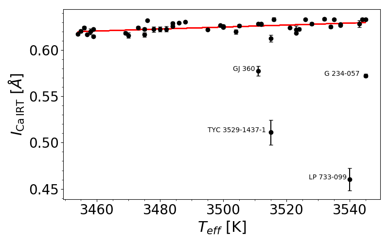
Figure 1: Average $I_{\mathrm{line}}$ in the Ca ii IRT line at $8500.35\,\AA$ against the $T_{\mathrm{eff}}$ of the investigated stars. The error bars correspond to the standard deviations of the line indices of individual spectra of the respective stars. The red line is a linear fit for the inactive stars exceeding $I_{\mathrm{Ca\,IRT}}=0.6\,\AA$. The four active stars are highlighted by their names.

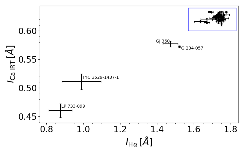
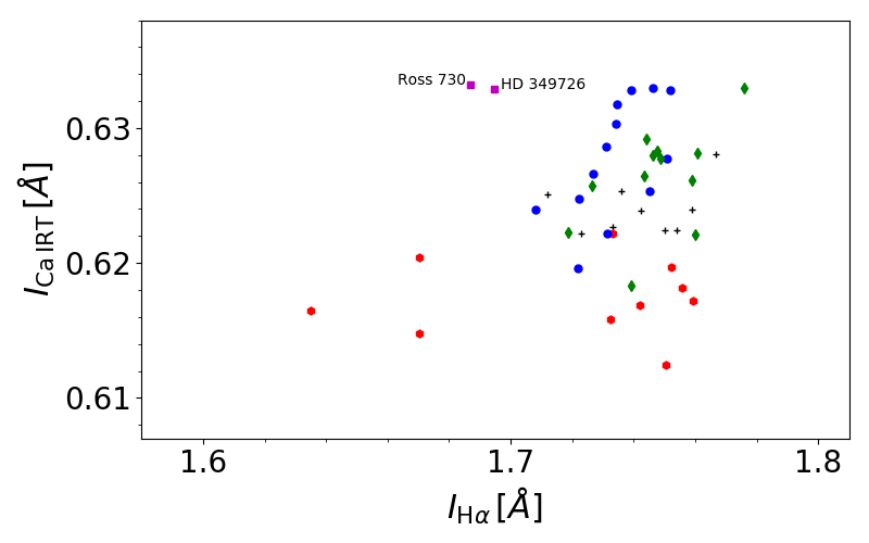
Figure 2: Upper panel: Average $I_{\mathrm{line}}$ in the Ca ii IRT line at $8500.35\,\AA$ against the average $I_{\mathrm{line}}$ in the H$\alpha$ line of the investigated stars. The error bars correspond to the standard deviations of the line indices of individual spectra of the respective stars. Lower panel: Zoom of the range of the inactive stars without error bars (blue box in the upper panel). The black pluses indicate the stars best fit by model #079, red hexagons indicate best fit by model #080, blue circles by #042, green diamonds by #047, and magenta squares by #029 (see Sect. 4.2). The model numbers and properties are given in Table LABEL:table_model_grid in the appendix. To improve clarity, the errors are faded out in the lower panel.

2.4 Activity characterization of the sample stars

The stars in the sample feature very different levels of stellar activity as can be easily seen qualitatively in the H$\alpha$ line, which is an absorption line for most of our sample stars, but goes into emission for four stars. The state of activity can be characterized quantitatively by the line index of chromospheric emission lines. Following the method of Fuhrmeister et al. (2018) and Robertson et al. (2016), the line index $I_{\mathrm{line}}$ is defined by

$$I_{\mathrm{line}}=w\left(1-\frac{\overline{F_{\mathrm{line}}}}{\overline{F_{\mathrm{ref1}}}+\overline{F_{\mathrm{ref2}}}}\right),$$ (1)

where $w$ is the bandwidth of the spectral line, and $\overline{F_{\mathrm{line}}}$, $\overline{F_{\mathrm{ref1}}}$, and $\overline{F_{\mathrm{ref2}}}$ indicate the mean flux densities of the spectral line and reference bands. The line index corresponds to the pseudo-equivalent width.

In this paper, we investigated the Na i D, H$\alpha$, and Ca ii IRT lines. These lines represent the most widely used chromospheric indicators in our wavelength range. Another known chromospheric line covered by our wavelength range is the He i D₃ line, which is seen in none of the spectra of our more inactive stars. Of the Na i D doublet and the Ca ii IRT triplet lines, we only considered the bluest components because the remaining lines are influenced in the same manner by the chromospheric structure. For the Ca ii IRT line we chose $w=0.5\,\AA$ to be the width of the line band centered at the (vacuum) wavelength of the line at $8500.35\,\AA$. The reference band located at the blue side of the Ca line is centered at $8481.33\,\AA$ with a half-width of $5\,\AA$, and the central wavelength of the red band is $8553.35\,\AA$ with a half-width of $1\,\AA$ to avoid telluric contamination for most radial and barycentric velocities. The center of the H$\alpha$ line band is located at a wavelength of $6564.62\,\AA$ and we chose the width of the line band to be $1.6\,\AA$. The reference bands are located at $6552.68\pm 5.25\,\AA$ and $6582.13\pm 4.25\,\AA$. For the Na i D₂ line at $5891.58\pm 0.2\,\AA$ the reference bands are $5872.3\pm 2.3\,\AA$ and $5912.0\pm 2.0\,\AA$.

Fig. 1 shows an overview of the activity levels and the spread in effective temperature of the stellar sample. Most of the stars are considered inactive indicated by the high Ca ii IRT index above $0.6\,\AA$, which should represent the average activity level of the star. The more active stars in our sample are GJ 360 and G 234-057 exhibiting line indices between $0.6\,\AA$ and $0.55\,\AA$ (further on also called semi-active), and even more active are LP 733-099 and TYC 3529-1437-1 with indices below $0.55\,\AA$. There is a photospheric trend to higher indices for higher effective temperatures marked as the linear fit in Fig. 1. This trend can also be found for the photospheric models by Husser et al. (2013) varying the effective temperatures between $3400$ and $3600\,$K ($\log g=5.0\,\mathrm{dex}$, $[\mathrm{Fe}/\mathrm{H}]=0.0\,\mathrm{dex}$ and $[\alpha/\mathrm{Fe}]=0.0\,\mathrm{dex}$). We used the index of the Ca ii IRT line to specify the different activity levels of the investigated stars, although in many studies, such as in Fuhrmeister et al. (2018), the line index of H$\alpha$ is used to determine the activity state. While the H$\alpha$ line is a strong line very sensitive to activity changes, the drawback in using the H$\alpha$ line is its evolution with increasing stellar activity: this line first goes into absorption, then fills up the line core and eventually goes into emission (see, e. g., Cram & Mullan, 1979). Thus more active stars can exhibit the same H$\alpha$ line index as less active stars. The Ca ii IRT line only fills in and goes into emission while the activity level increases, making its index easier to interpret in terms of the activity state.

In Fig. 2 we compare the average line indices of the Ca ii IRT line and the H$\alpha$ line that are given in Table 1. The plot exhibits a good correlation between the two indices with a Pearson correlation coefficient of $0.97$, while the indices of the more inactive stars form an uncorrelated cloud. At the highest Ca ii IRT line indices there are two stars, Ross 730 and HD 349726, exhibiting lower H$\alpha$ indices; we interpret these to be the most inactive stars of the sample being located in the branch where increasing activity means increasing H$\alpha$ line depth. As error bars we plot the standard deviation of the line indices derived from individual spectra of the respective stars. The scatter in the H$\alpha$ line index is obviously larger than that in the Ca ii IRT line. So the H$\alpha$ line appears to be more sensitive for activity variations in the whole observation period. This supports the choice for the Ca ii IRT line index as a robust estimate of the mean activity level of a given star. For further insight into the variability of individual stars we show the time series of the three considered lines for TYC 3529-1437-1 in Fig.  3 as one of the stars with the largest amount of variations. Fig.  3 demonstrates the typical temporal sampling of the spectral time series, which has been optimized for planet searches. The average sampling cadence is around 14 days. Also times of different levels of activity can be identified: the star was more active at the end of the time series. Since we do not want to average the variations of the lines or whole periods of enhanced activity, we do not co-add the observations. Co-adding would certainly boost the signal-to-noise ratio, but most stars also have signal-to-noise ratios above 50 in single spectra, which is sufficient for our analysis. Therefore, we examine the spectrum with the median line index $I_{\mathrm{Ca\,IRT}}$ as a representation of the median activity level of the star. For the inactive stars the level of variation is much lower and an averaging would be possible in the sense of not mixing different activity states, but for consistency we treat these like the four active stars.

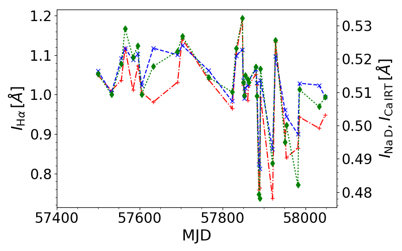
Figure 3: Time series of the indices $I_{\mathrm{line}}$ of the Na i D₂ (blue crosses), H$\alpha$ (red pluses), and Ca ii IRT line (green diamonds) of TYC 3529-1437-1.

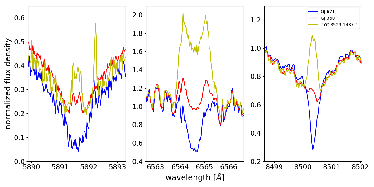
Figure 4: Example spectra of one inactive (GJ 671, blue line), one semi-active (GJ 360, red line), and one very active star (TYC 3529-1437-1, yellow line) in the stellar sample in the range between Na i D₂, H$\alpha,$ and the bluest Ca ii IRT line. The peak right to the sodium line of TYC 3529-1437-1 is an airglow line.

In Fig. 4 we show individual example spectra of one inactive (GJ 671) and two active stars (GJ 360, TYC 3529-1437-1). The inactive star exhibits absorption lines in Na i D₂, H$\alpha$, and the bluest Ca ii IRT line. For GJ 360 the spectral lines are in the transition from absorption to emission, while the lines in the spectrum of TYC 3529-1437-1 are clearly in emission. Thus we cover the bandwidth of rather inactive, semi-active, and very active M dwarfs in our sample.

3 Model construction

The state-of-the-art PHOENIX code models atmospheres and spectra of a wide variety of objects such as novae, supernovae, planets, and stars (Hauschildt, 1992, 1993; Hauschildt & Baron, 1999). A number of PHOENIX model libraries covering M dwarfs have been published. For instance, Allard & Hauschildt (1995) used local thermodynamic equilibrium (LTE) calculations for dwarfs with effective temperatures of $1500\,\mathrm{K}\leq T_{\mathrm{eff}}\leq 4000\,\mathrm{K}$ and Hauschildt et al. (1999) computed an even wider model grid in the temperature range between $3000\,$K and $10000\,$K. A recent library of PHOENIX model atmospheres was presented by Husser et al. (2013).

3.1 Selection of a photospheric model

All of the above-mentioned libraries are exclusively concerned with the photospheres. The first model calculations that investigated the chromospheres using PHOENIX were carried out by Short & Doyle (1997) and Fuhrmeister et al. (2005). These models extend the atmospheric range up to the transition region, but are still rooted in the atmospheric structure of the photosphere, which therefore, provides the basis for our calculations.

In this paper, we adopt a photospheric model from the Husser et al. (2013) library as the underlying photosphere. This model was calculated under the assumptions of spherical symmetry and LTE using 64 atmospheric layers. The particular model atmosphere we adopted was computed for the parameters $T_{\mathrm{eff}}=3500\,\mathrm{K}$, $\log g=5.0\,\mathrm{dex}$, $[\mathrm{Fe}/\mathrm{H}]=0.0\,\mathrm{dex,}$ and $[\alpha/\mathrm{Fe}]=0.0\,\mathrm{dex}$; in Fig. 5 (blue line) we show the temperature as a function of column mass for this model photosphere. Obviously, the temperature decreases continuously outward.

3.2 Chromospheric models

We now extend the photospheric model following the approach of Short & Doyle (1997) and Fuhrmeister et al. (2005). In particular, we add three sections of rising temperature to the model photosphere, which represent the lower and upper chromosphere and the transition region. To technically facilitate the extension, we increase the number of atmospheric layers in the model from originally 64 to 100 layers.

Our model chromosphere is described by a total of six free parameters. The column mass density at the onset of the lower chromosphere, $m_{\mathrm{min}}$, defines the location of the temperature minimum. The column mass densities and temperatures of the end points of the lower ($\log m_{\mathrm{mid}}$, $T_{\mathrm{mid}}$) and the upper chromosphere ($\log m_{\mathrm{max}}$, $T_{\mathrm{max}}$), and the temperature gradient in the transition region, $grad_{\mathrm{TR}}$, given by

$$grad_{\mathrm{TR}}=\frac{d\,T}{d\,\log\,m}={\rm const.}$$ (2)

as introduced by Fuhrmeister et al. (2005). The maximum temperature of the transition region is fixed at $T_{\mathrm{TR}}=98\,000\,$K. The temperature rise segments in the lower, upper chromosphere, and transition region are taken to be linear in the logarithm of the column mass density in our model. This is a rough approximation to the structure of the VAL C model. The meaning of the individual parameters is also illustrated in Fig. 5, where we show the temperature structure of the original photospheric model along with a modified structure including the photosphere, chromosphere, and transition region.

We used this modified temperature structure as a new starting point for the PHOENIX calculations. To account for the conditions in the chromosphere, the atomic species of H i, He i $-$ ii, C i $-$ ii, N i $-$ v, O i $-$ vi, Na i $-$ ii, Mg i $-$ ii, K i $-$ ii, and Ca i $-$ iii are computed in non-LTE (NLTE) for all available levels taken from the database of Kurucz & Bell (1995). This applies to all species but He, for which we consulted CHIANTI v4 (Landi et al., 2006). The PHOENIX code iteratively adapts the electron pressure and mean molecular weight to reconcile these with the NLTE H i/H ii ionization equilibrium. To that end, it is necessary that the population of all the states of the NLTE species are reiterated with the photoexciting and photoionizing radiation field, which is particularly important in the thin chromospheric and transition region layers. Moreover, the electron collisions have to be taken into account. A detailed comparison between LTE and NLTE atmospheric models is described by, for example, Short & Hauschildt (2003). Our calculations rely on the assumption of complete redistribution, as PHOENIX does not yet support partial redistribution, which would provide a more appropriate treatment in large parts of the chromosphere. However, its expected impact is largest for the Ly$\alpha$ line and resonance lines such as the Ca ii H and K line, which we also do not use in our study; the Na i D lines are much less affected (Mauas, 2000).

Figure 5: Photosphere model (blue solid line) at $T_{\mathrm{eff}}=3500\,$K, $\log g=5.0\,\mathrm{dex}$, $\left[\mathrm{Fe}/\mathrm{H}\right]=0\,\mathrm{dex,}$ and $\left[\alpha/\mathrm{Fe}\right]=0\,\mathrm{dex}$ taken from the Husser et al. (2013) library and an attached chromosphere model consisting of linear sections (red dashed line). The arrows indicate the variable parameters of the chromosphere model.

Table 2: Parameter ranges for the chromosphere models.

Parameter	Minimum value	Maximum value
$m_{\mathrm{min}}\,[\mathrm{dex}]$	$-4.0$	$-0.3$
$m_{\mathrm{mid}}\,[\mathrm{dex}]$	$-4.3$	$-1.5$
$T_{\mathrm{mid}}\,[\mathrm{K}]$	$3500$	$8000$
$m_{\mathrm{top}}\,[\mathrm{dex}]$	$-6.0$	$-3.5$
$T_{\mathrm{top}}\,[\mathrm{K}]$	$4500$	$8500$
$grad_{\mathrm{TR}}\,[\mathrm{dex}]$	$7.5$	$10.0$

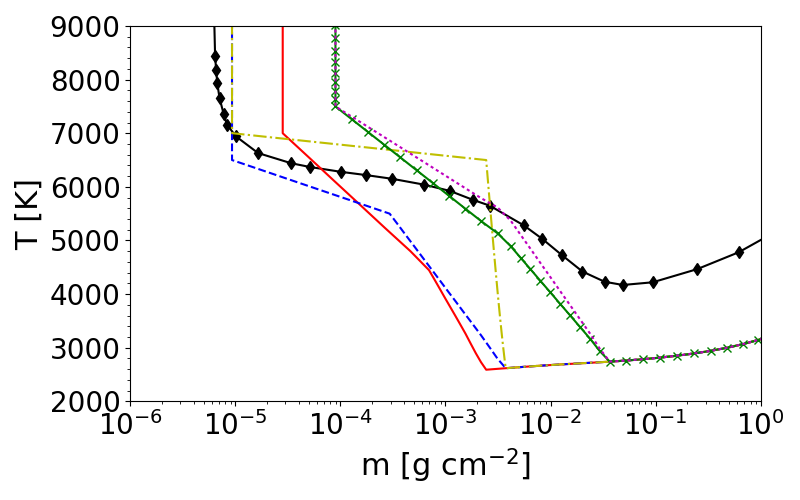
Figure 6: Upper panel: Temperature structure of the best single-component fits for the inactive stars as listed in Table 3 in the appendix. Model #029 is shown by the red solid line, #042 by the blue dashed line, #047 by the yellow dash-dotted line, #079 by the green crossed line, and #080 by the magenta dotted line. Lower panel: Same as in the upper panel for the active stars. Model #131 is plotted by the red solid line and #136 by the blue dashed line. The black solid diamond line shows the VAL C model for the Sun (Vernazza et al., 1981).

3.3 Hidden parameters

Besides the six parameters describing the temperature structure introduced in Sect. 3.2, there are further aspects of the model that can be modified and influence the solution, most importantly, the microturbulence and the chosen set of NLTE lines.

While in our models the photospheric microturbulent velocity is set to $2\,\mathrm{km}\,\mathrm{s}^{-1}$, in the chromosphere and the transition region the velocity is set to half the speed of sound in each layer, but is not allowed to exceed $20\,\mathrm{km}\,\mathrm{s}^{-1}$ which may otherwise happen in the transition region. This follows the ansatz by Fuhrmeister et al. (2005). We do not smooth the microturbulent velocity transition between photosphere and chromosphere but the conditions in the model lead to quasi-smooth transitions with increases between two layers not exceeding $3\,\mathrm{km}\,\mathrm{s}^{-1}$. Varying the microturbulent velocity leads to changes in the intensity as well as in the shape of the spectral lines (Jevremović et al., 2000). The considered NLTE set is practically restricted by the computational effort. While a more comprehensive NLTE set including, for example, higher O and Fe species would certainly be desirable to improve the synthetic spectra, we consider the here-adopted NLTE set sufficient to model the chromosphere in the context of the investigated lines.

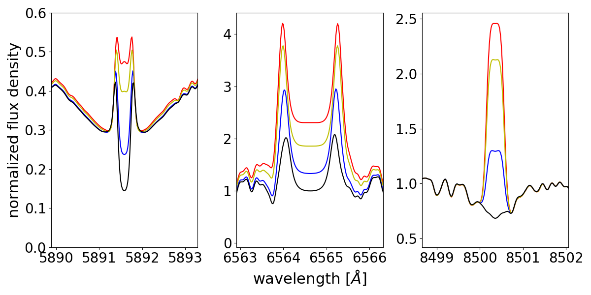
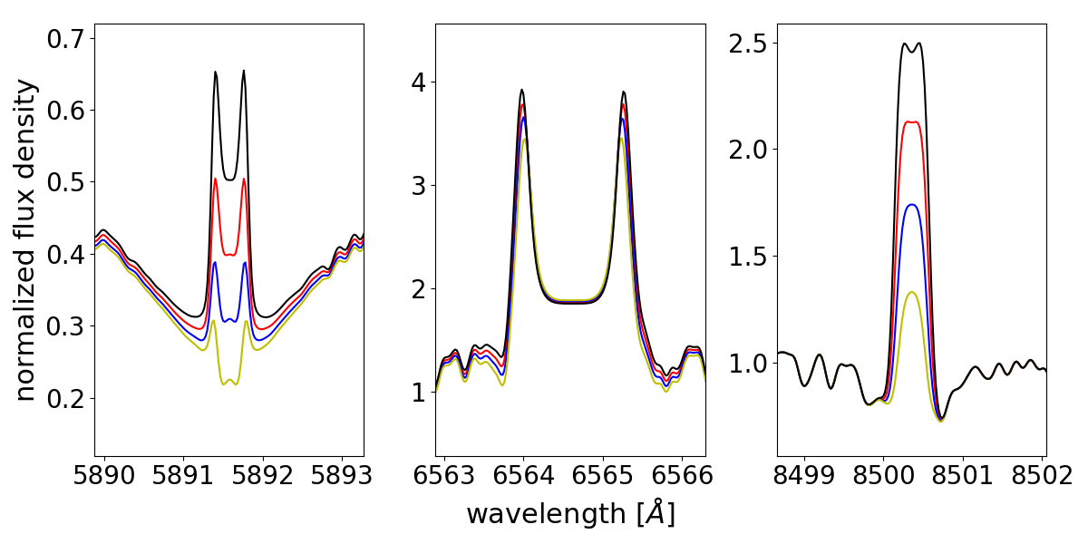
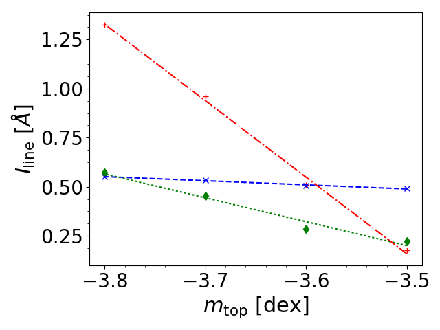
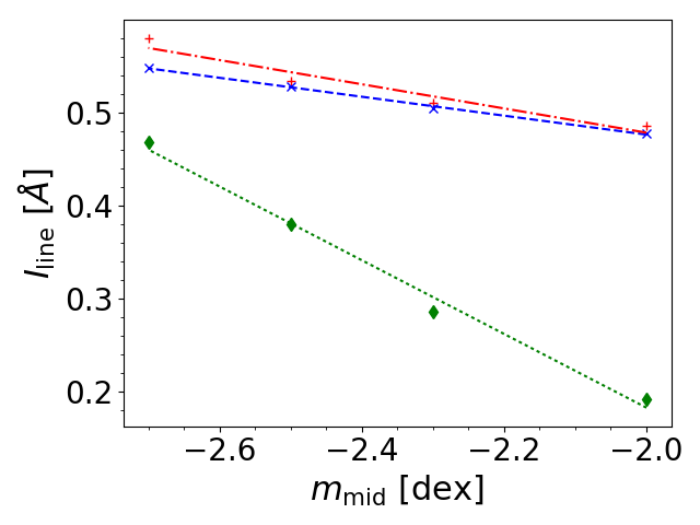
Figure 7: Top panel: left-hand side: Sequence of model spectra varying only the parameter $m_{\mathrm{top}}$ from $-4.0$ to $-3.5\,$dex, the models are: #136 (black), #137 (blue), #138 (yellow), and #139 (red). Right-hand side: Sequence for the parameter $m_{\mathrm{mid}}$ varying from $-2.7$ to $-2.0\,$dex, models: #121 (yellow), #126 (blue), #138 (red), and #153 (black). Bottom panel: Corresponding values of $I_{\mathrm{line}}$ against $m_{\mathrm{top}}$ for Na i D (blue crosses), H$\alpha$ (red pluses), and Ca ii IRT (green diamonds) for the top panels. Additionally the linear fits are plotted: the Na i D fit is plotted by the blue dashed line, the H$\alpha$ fit by the red dash-dotted line, and the Ca ii IRT fit by the green dotted line.

3.4 The model set

Our chromospheric model is described by six free parameters, and as a result of the rather large NLTE sets, each model calculation requires several dozens of CPU hours. While it may seem most straightforward to obtain a model grid homogeneously covering typical ranges for all free parameters, already a very moderate sampling of ten grid points per free parameter results in a grid with $10^{6}$ elements, which results in too high a computational demand. It is also clear that the large majority of the grid points are expected to result in spectra nowhere near the observations, which would be of little use in the subsequent analysis.

The challenge was therefore to identify reasonable parameter ranges and to explore these with a number of models. To that end, we first calculated limiting cases, such as models simultaneously showing all spectral lines in absorption or emission, in other words inactive or active chromosphere models. By visual comparison with the observed spectra, we subsequently identified the most promising parameter ranges to be explored further.

A particularly interesting comparison is between models with a steep temperature rise in the lower chromosphere and a plateau in the upper chromosphere, and models with a shallow temperature increase in the lower chromosphere and a steeper increase in the upper chromosphere. The first type of model is similar in structure to the VAL models used for the Sun.

The final set of models used in this study comprises 166 models with different model parameter configurations. The parameters are varied in the ranges listed in Table 2, and the properties of the individual models are given in Table LABEL:table_model_grid in the appendix. The activity levels of the models are given by the line index $I_{\mathrm{Ca\,IRT}}$ but, as shown in Sect. 3.6 and Sect. 3.7, H$\alpha$ can behave differently compared to the Ca ii IRT. Figure 6 shows an excerpt of the model set. Three models have steep gradients in the lower chromosphere and shallow gradients in the upper chromosphere, and it turns out these models represent more inactive states. The other three models have the shallow gradients in the lower and the steep gradients in the upper chromosphere and are rather characteristic of active chromospheres.

3.5 Synthetic high-resolution spectra

To compare our models to stellar spectra, we need densely sampled synthetic spectra. We calculated the synthetic spectra in the spectral ranges of $3900$–$4000\,\AA$, $4830$–$4890\,\AA$, $5700$–$7000\,\AA$, and $8000$–$8800\,\AA$ with a sampling of $\Delta\lambda=0.005\,\AA$ per spectral bin. These ranges comprise the chromospheric lines covered by CARMENES as discussed in Sect. 2.4 and additionally the Ca ii H and K, H$\epsilon$, and H$\beta$ lines to enable a comparison to spectra obtained by other instruments such as the High Accuracy Radial velocity Planet Searcher (HARPS; Mayor et al., 2003) in the context of further investigations. For the comparison to the CARMENES spectra, we lowered the model spectral resolution to that of CARMENES by folding with a Gaussian kernel of the approximated width. The stellar rotational velocities are neglected because none of the sample stars is a fast rotator with v $\sin i$ never exceeding $4\,\mathrm{km}\,\mathrm{s}^{-1}$ (Reiners et al., 2017; Jeffers et al., 2018). Even for the most active stars in our sample, relatively long rotation periods are not in contradiction with their activity. Newton et al. (2017) found the threshold between active and inactive stars (H$\alpha$ in emission or absorption) for early M dwarfs to be at a rotation period of about $30\,$days. For two of our active dwarfs we have rotation period measurements by Díez Alonso et al. (2019): GJ 360 has a period of $21\,$days and TYC 3529-1437-1 has a period of $15.8\,$days. These periods are consistent with the corresponding v $\sin i$ values and there is no need to assume that they are seen pole-on.

3.6 Sequences modeling the evolution of the chromospheric lines

The interaction of the parameters determines whether the chromospheric lines are in absorption or emission and determines the strengths and shapes of the lines. In order to obtain an impression of how variations of a single parameter affect the line properties, we show in Fig. 7 the lines of Na i D₂, H$\alpha$, and the blue Ca ii IRT line of different models only varying in the parameter $m_{\mathrm{top}}$ from $-4.0$ to $-3.5\,$dex (left-hand side) and in $m_{\mathrm{mid}}$ from $-2.7$ to $-2.0\,$dex (right-hand side). Changing a parameter of the upper chromosphere leads to stronger effects for H$\alpha$ compared to Na i D and Ca ii IRT, although the Ca ii IRT is clearly more influenced than Na i D. The line indices illustrated in the lower panel confirm this impression with the gradients of the linear fits. However, the line core of Na i D₂ is filled up while the peaks are increasing less. The H$\alpha$ and Ca ii IRT lines completely go from absorption to emission, and simultaneously the H$\alpha$ self-absorption becomes even stronger.

While H$\alpha$ is almost not influenced by the variation of $m_{\mathrm{mid}}$, the Ca ii IRT emission peak is approximately four times higher above the continuum for $m_{\mathrm{mid}}=-2.0\,$dex than for $m_{\mathrm{mid}}=-2.7\,$dex. The variation of Na i D is also visible in the spectra, but not as strong as for the Ca ii IRT line. The strong self-absorption of Na i D leads to a smaller variation of the line index than for the Ca ii IRT. This sequence suggests a weak relationship of the H$\alpha$ formation to the mid-chromosphere, while the other two lines clearly depend on the structure of the transition between lower and upper chromosphere.

Furthermore, we also found the location $m_{\mathrm{min}}$ of the temperature minimum of the chromosphere to be a decisive factor to determine whether lines appear in absorption or emission. More active lines are generated with a temperature minimum at higher density as found by Short & Doyle (1998) who calculated a model grid for the chromospheric lines of H$\alpha$ and Na i D in five M dwarfs.

3.7 Flux contribution functions

Performing sequences indicates that modeling the chromospheric lines of Na i D₂, H$\alpha$, and the bluest Ca ii IRT line turns out to be a challenge mainly due to different formation heights of the line wings and cores in the chromosphere. Therefore, we investigated where the lines form in order to improve the understanding of the chromospheric structure and to make restrictions for the calculations of the chromospheres. The PHOENIX code is capable of computing flux contribution functions following the concept of Magain (1986) and Fuhrmeister et al. (2006). The intensity contribution function $\mathscr{C}_{I}$ is defined by

$$\mathscr{C}_{I}(\log m)=\mu^{-1}\,\ln 10\,m\,\kappa\,S\,e^{-\tau/\mu},$$ (3)

where $m$ is the column mass density, $\kappa$ the absorption coefficient, $S$ the source function, $\tau$ the optical depth, and $\mu=\cos\theta$, with $\theta$ as the angle between the considered direction and surface normal. The flux contribution function $C$ is the intensity contribution function integrated over all $\mu$ and it gives information on where the flux density of every computed wavelength in the stellar atmosphere arises from. Fig. 8 illustrates the flux contribution function of the line core (upper panel) and wing (mid-panel) of the bluest Ca ii IRT line for model #080 (see Table LABEL:table_model_grid). Additionally, the source function $S_{\nu}$, Planck function $B_{\nu}$, and intensity $J_{\nu}$ are given in the plots. The core is formed nearly at the center of the upper chromosphere at $T=6200\,$K. In the lower panel the temperature structure of the model is shown to visualize at which temperatures the lines are formed and the formation regions of Na i D₂, H$\alpha$ and the Ca ii IRT line are given. The formation region is defined as the full width at half maximum around the maximum of the contribution function above the photosphere. The Na i D₂ core is formed in the transition between the lower and upper chromosphere at $T=5800\,$K, while the H$\alpha$ core is formed at the top of the chromosphere at $T=13700\,$K. This is in agreement with the results from the best-fit model by Fuhrmeister et al. (2005) for AD Leo in Na i D and H$\alpha$.

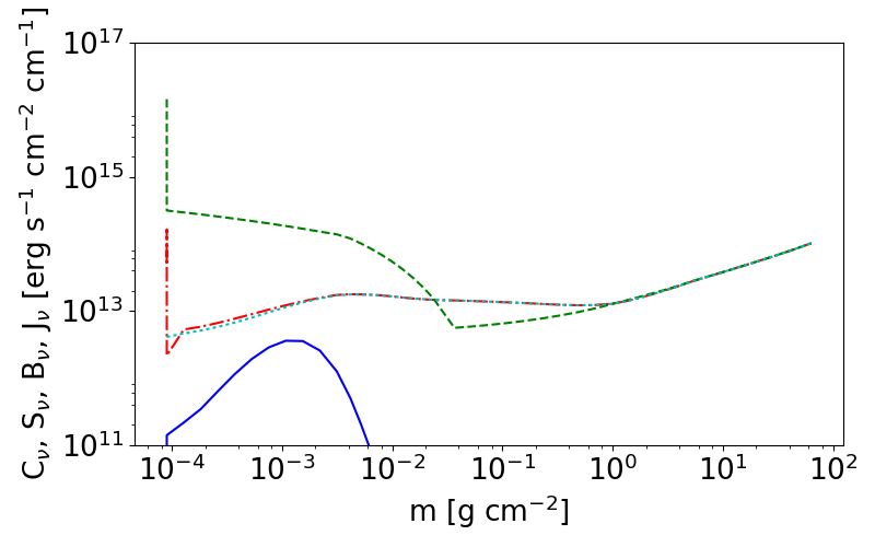
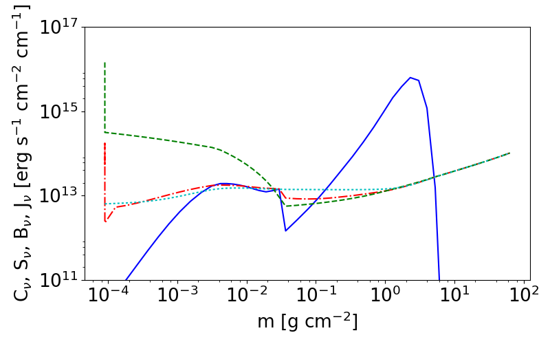
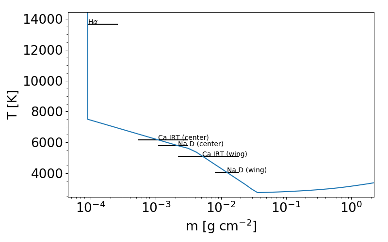
Figure 8: Upper and mid-panels: Scaled flux contribution function $C_{\nu}$ (solid blue), source function $S_{\nu}$ (dash-dotted red), Planck function $B_{\nu}$ (dashed green), and intensity $J_{\nu}$ (dotted cyan) for $\lambda=8500.36\,\AA$ representing the line core (upper panel) and $\lambda=8500.54\,\AA$ in the line wing (mid-panel) of the Ca ii IRT line in model #080. The peak at high column mass in the contribution function of the line wing shows that the photospheric flux already dominates at this wavelength but there is still some chromospheric contribution. Lower panel: Temperature structure of model #080 and the formation regions of Na i D₂, H$\alpha$, and the bluest Ca ii IRT line.

4 Results and discussion

4.1 Comparing synthetic and observed spectra

To compare our synthetic spectra to observations we focus on the Na i D₂, H$\alpha$, and the bluest Ca ii IRT lines. Before carrying out the comparison, the flux densities of the observed and synthetic spectra were normalized to the mean value in the blue reference bands of the respective chromospheric line (see Sect. 2.4). For stars with several available spectra, we used the spectrum with the median value of the $I_{\mathrm{Ca\,IRT}}$ line index for comparison.

Our comparison is based on a least-squares-like minimization. In particular, we consider the difference between the observed and synthetic spectra simultaneously in the wavelength ranges $\lambda_{\mathrm{NaD}}\pm 0.2\,\AA$, $\lambda_{\mathrm{H\alpha}}\pm 0.8\,\AA$ and $\lambda_{\mathrm{CaIRT}}\pm 0.25\,\AA$. These line bands cover the chromospheric cores of the respective spectral lines. In Fig. 9 we show the best-fit models to the individual lines of TYC 3529-1437-1 irrespective of the other two lines. In the case of the Ca ii IRT line, the best-fit model (yellow line) produces an almost perfect match to the observed line core, however, a comparison of this model to the shape of Na i D and H$\alpha$ shows clear mismatches with regard to the data. While the predicted H$\alpha$ line shows too strong an emission, the core of the associated Na i D line profile is strongly absorbed, which is clearly at odds with the observation. However, it is possible to obtain good fits for each of the three lines individually using appropriate models.

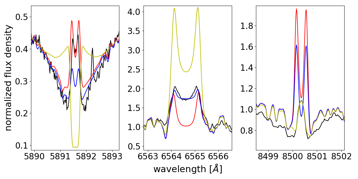
Figure 9: Comparison of the observed median activity spectrum of TYC 3529-1437-1 (black) as given by $I_{\mathrm{Ca\,IRT}}$ to the model spectrum fitting best in a single line. Best-fit models using only Na i D₂ are denoted in red (model #078), using only H$\alpha$ in blue (model #073), and Ca ii IRT in yellow (model #157).

For physical reasons, the line band used for the H$\alpha$ line is nearly three times as wide as that of the Ca ii IRT line and four times wider than that of the Na i D₂ line. Moreover, the observed (and modeled) amplitude of variation in these line profiles is by far largest for the H$\alpha$ line. Both factors boost the weight of the H$\alpha$ line profile in the minimization based on the summed $\chi^{2}$ values obtained in the three line bands as the objective. This reflects a relative overabundance of data in the H$\alpha$ line and makes it the dominant component in such a fit. However, we intend to find the model that provides the most appropriate representation of all three considered chromospheric lines simultaneously.

Therefore, we constructed a dedicated statistic, $\chi^{2}_{m}$, which we use as the objective function in our minimization. Specifically, we define

$$\chi^{2}_{m}=\chi^{2}_{\rm H\alpha}+w_{\rm Na}\,\chi^{2}_{\rm Na}+w_{\rm Ca}\,\chi^{2}_{\rm Ca}\;,$$ (4)

where $\chi^{2}_{\rm H\alpha}$, $\chi^{2}_{\rm Na}$, and $\chi^{2}_{\rm Ca}$ denote the sum of squared differences between model and observation obtained in the individual line bands. The weighting factors $w_{\rm Na}$ and $w_{\rm Ca}$ were adapted to give approximately the same weight to all three lines in the minimization. To counterbalance the different widths of the line bands we increase the weighting of the Na i D₂ and Ca ii IRT line bands by a factor of $3$. To account for the different flux density scales of variation in the Na i D₂ and Ca ii IRT lines, an additional factor of $4$ is added to further increase their weight. The factor of 4 was estimated based on the observed amplitude of variation of the H$\alpha$ line compared to the variation of the Na i D₂ and Ca ii IRT lines. We therefore end up with weighting factors of $w_{\rm Na}=w_{\rm Ca}=12$. The resulting $\chi^{2}_{m}$ statistic establishes a relative order among the model fits, but cannot be used as a goodness-of-fit criterion.

4.2 Single-component fits

In a first attempt, we directly compare our set of synthetic spectra with the observations using the modified $\chi^{2}_{m}$ criterion defined above. Since we normalize both the model and observation using the same reference band, no free parameters in this comparison remain; however, we compare every observed spectrum to all spectra from our set of models. Table 3 in the appendix lists the results of the single model fits for the whole stellar sample, i. e., the models with the lowest modified $\chi^{2}_{m}$ value. An inspection of Table 3 shows that this approach yields reasonable fits with $\chi^{2}_{m}$ values between 1.8 and 4.04 for most stars, while four stars, the outliers in Fig. 1, show only poor fits with $\chi^{2}_{m}$ values in excess of 10.

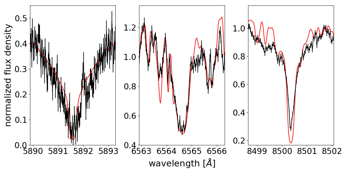
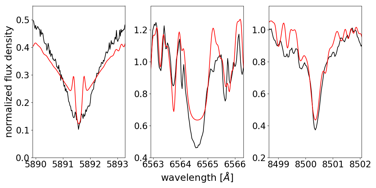
Figure 10: Comparison of the best-fit model spectrum (red) to the observed spectrum (black) with median activity as defined by $I_{\mathrm{Ca\,IRT}}$. Upper panel: GJ 671 and model #042. Lower panel: EW Dra and model #080.

4.2.1 Inactive stars

For the inactive stars in our sample interestingly a small subset of five models provides the best fits, viz., the models #029 (2 cases), #042 (13 cases), #047 (12 cases), #079 (9 cases), and #080 (10 cases). In the lower panel of Fig. 2, the distribution of inactive stars is shown in the plane spanned by the H$\alpha$ and Ca IRT activity indices. The color coding identifies the best-fitting models from Table 3. While for most of the stars with $I_{\mathrm{Ca\,IRT}}<0.625$ model #080 is the best from our set, the spectra of the majority of stars exceeding this value are best represented by model #042. The two stars Ross 730 and HD 349726, which we consider the most inactive in our sample (see Sect. 2.4), are best represented by model #029. The modified $\chi^{2}_{m}$ values range between $1.8$ and $4.5$ for the inactive stars.

As an example, we juxtapose the best-fitting models and observed spectra of the two inactive stars GJ 671 and EW Dra in Fig. 10. In these models as well as in the observations all the considered lines appear in absorption. We note that the observation of the sodium line of GJ 671 shows some telluric emission, however, sufficiently offset from the line core. From our point of view, the #042 provides a reasonable fit to all considered lines in the case of GJ 671. Despite some shortcomings, such as a too deep Ca IRT line in the model and a somewhat too narrow sodium trough, all aspects of the data are appropriately reproduced by the model spectrum.

For the case of EW Dra, the overall situation is less comfortable. The strongest deviation of model #080 from the observed spectrum of EW Dra is the width of the central part of the Na i D₂ line. The model clearly produces a too wide line with a signature of a central fill-in and self-absorption clearly more pronounced than in the observation. We emphasize, however, that despite these differences, the observation shows a similar structure in the line core, yet of course less pronounced. The line shapes of the H$\alpha$ and the Ca ii IRT line are well represented by this model although in particular the observed H$\alpha$ line is deeper than that predicted by the model.

Although there are shortcomings, we conclude that the spectra of inactive stars can be appropriately represented by our models. Notably, all best-fit models for inactive stars are characterized by a temperature structure with a steeper temperature rise in the lower chromosphere and a more shallow rise in the upper chromosphere. This is in fact not very different from the VAL C model (Vernazza et al., 1981) for the Sun, which also shows a steeper temperature rise in the lower chromosphere and a plateau in the upper chromosphere.

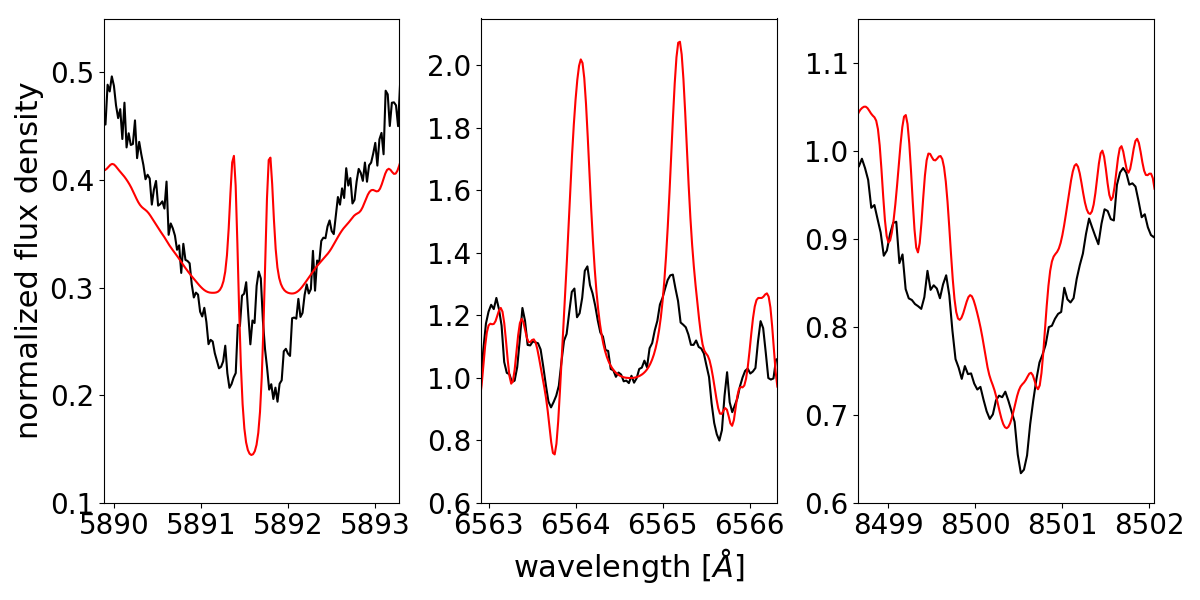
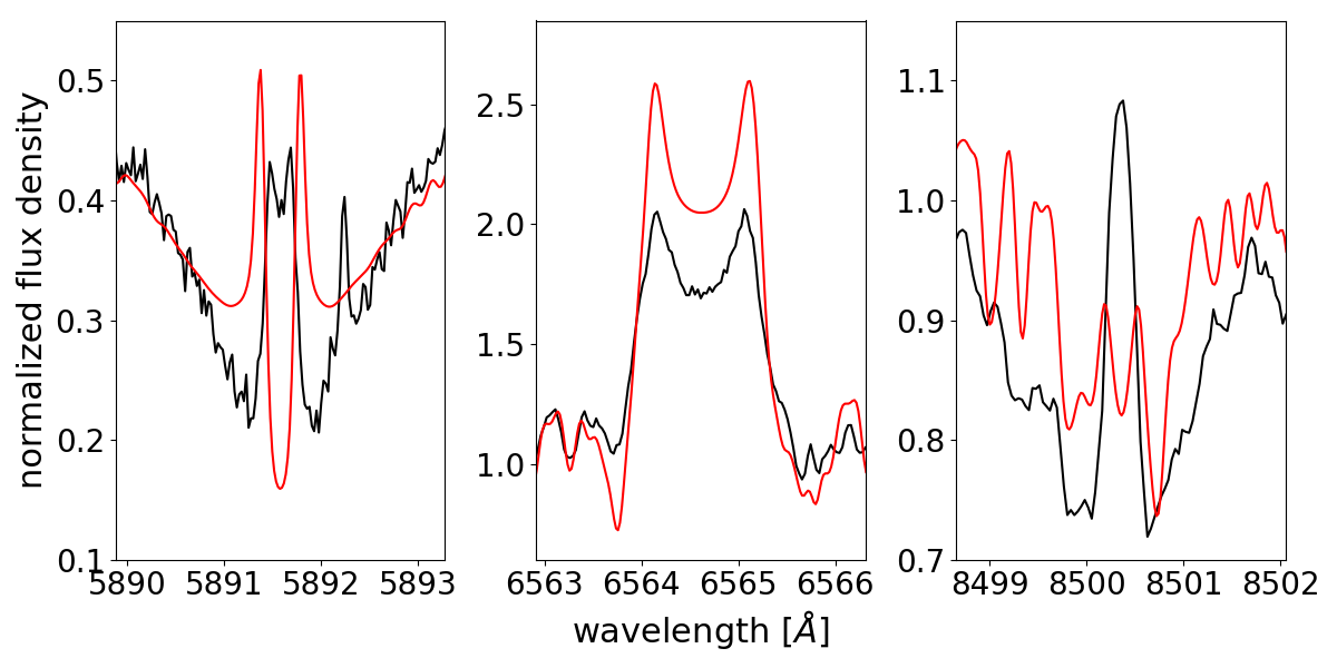
Figure 11: Same as Fig. 10. Upper panel: GJ 360 and model #136. Lower panel: TYC 3529-1437-1 and model #131.

4.2.2 Active stars

For the active stars in our sample we only need two models that provide the best fits, viz., the models #131 (2 cases) and #136 (2 cases). In Fig. 11 we show the observed spectra and best-fit models for the more active stars GJ 360 and TYC 3529-1437-1, and clearly, in both cases the modified $\chi^{2}_{m}$ values are more than twice as high as for any inactive star in the sample. The observed Na i D line profiles show self-absorption in both stars, which is also predicted by the model, but the width of the emission core is too broad for the models and the self-absorption is too strong. The observed H$\alpha$ lines of both stars show clear self-absorption. This aspect is reproduced by the models, although for GJ 360 the model strongly overpredicts the self-absorption. The overall H$\alpha$ line profile seems more appropriate for TYC 3529-1437-1, although the model yields a line that is too strong. The shape of the Ca ii IRT line in the model is roughly reproduced in GJ 360; the model for TYC 3529-1437-1 shows considerable self-absorption, which is not observed. In particular for the more active stars, it is hard to fit all three lines simultaneously by one model.

The column mass densities of the temperature minima $m_{\rm min}$ of the best-fit models of the active stars are obviously higher compared to the models of the inactive stars. Both models have a density of at least $\Delta m_{\rm min}=0.5\,$dex higher than the found inactive models. In notable contrast to our results for the inactive stars, the best-fit models for the spectra of the more active stars tend to show a more shallow rise in the lower chromosphere and a steeper rise in the upper chromosphere. It is possible to increase the flux of the H$\alpha$ and Na i D₂ lines by only moving the chromosphere to increasing densities, but the shape of the chromosphere needs to be changed to reconcile a more active chromosphere with the Ca ii IRT line. Although this result has to be viewed against the background of the shortcomings of the fit, we tentatively identify this reversal of gradients as a characteristic change in the chromospheric temperature structure associated with a change from an inactive to an active chromosphere.

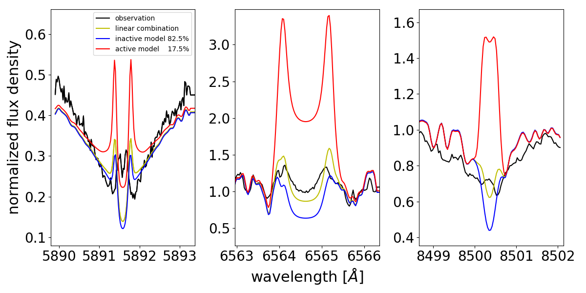
Figure 12: Comparison of the observed median activity spectrum to the best linear-combination fits for GJ 360 (upper panels, inactive model #080 and active model #132) and TYC 3529-1437-1 (lower panels, inactive model #079 and active model #149). The line of Na i $\mathrm{D}_{2}$ and the bluest Ca ii IRT line are weighted by a factor of $12$, respectively, compared to H$\alpha$ as described in Sect. 4.1.

4.3 Linear-combination fits

The solar chromospheric spectrum is well known for varying across the solar disk, in particular, when active regions and quiet regions are compared. To account for this fact, some studies using one-dimensional static models have combined models applying a filling factor. This method was first applied using models with a thermal bifurcation by Ayres (1981) to account for observations of molecular CO in the solar spectrum. However, it cannot be explained by chromospheric models alone, which have a temperature minimum well above a temperature allowing for CO. Such studies normally use linear combinations of a photospheric (or inactive chromospheric) and an active chromospheric model and have also been used for flare modeling (Fuhrmeister et al., 2010). Classically this treatment is also known as 1.5D modeling, since it tries to account for the inhomogeneity of the stellar atmospheres (Ayres et al., 2006). It relies on the assumption that the individual components are independent and influence each other neither radiatively nor collisionally via NLTE. This assumption would be satisfied if these regions were optically thick, which they are most probably not, but neither are they too optically thin. Therefore, we consider the assumption to be approximately satisfied.

We also adopt this approach in an attempt to improve especially the spectral fits of the more active dwarfs in our sample. In particular, we consider a linear combination of an inactive and an active spectral model, and determine a best-fit filling factor by again minimizing the modified $\chi^{2}_{m}$ value. This analysis is done for the whole stellar sample from Table 1, and Table 4 summarizes the results. The latter table contains the filling factors of the inactive and active component and the associated modified $\chi^{2}_{m}$ values. Although these values do not represent classical $\chi^{2}$ value, they can be compared with those of the single model fits (see Table 3). As expected, the modified $\chi^{2}_{m}$ values improve for every star when a second component is added to the model. Table 4 also lists the differences of the Ca ii IRT line indices ($\Delta I_{\mathrm{Ca\,IRT}}$) between the inactive and active model in the best combination fits giving an impression of the contrast in the respective combinations.

4.3.1 Inactive stars

In the spectral fits of the inactive sample stars, we start with the best-fit single-component model as the first component. We then add every model of our model set, determine a best-fit filling factor, and finally, choose the model combination providing the minimum modified $\chi^{2}_{m}$. The thus determined second model component mostly also exhibits the Na i D₂, H$\alpha$ and the Ca ii IRT lines in absorption. Although the combination leads to better matching of the line shapes, the overall improvement obtained for the inactive stars remains moderate.

4.3.2 Active stars

The spectra of the active stars could not be reproduced well with our single-component fits. Therefore, we do not consider the best-fit single model component as a good starting point for the fit as for the inactive stars and, instead, apply the following procedure. As the inactive spectral model component, we subsequently tested the five models, which produced the best fits for the inactive stars in the single-component approach (see Sect. 4.2). These were then tentatively combined with all other models from our set and the filling factor determined. Again, we finally opted for that combination providing the minimum modified $\chi^{2}_{m}$ value.

The best $\chi_{m}^{2}$ value is obtained by the combination with models with differences regarding the temperature structure in comparison to the found inactive models. The temperature gradient of the lower chromosphere is shallower and that of the upper chromosphere is steeper, which is the reverse case for the five best models of the inactive stars. While the active models of G 234-057 and GJ 360 have higher gradients in the upper than in the lower chromosphere, in the active model of LP 733-099 and TYC 3529-1437-1 the gradients of the lower and upper chromosphere are equal, meaning the chromosphere consists of only one linear section. Furthermore, in each of these active models the whole chromosphere is shifted inward about $\Delta m=0.5\,$dex compared to the inactive models. The width of the chromosphere nearly remains the same in every case, but the temperature at the top of the chromosphere increases at least by about $300\,$K. The interaction of the free parameters yields chromospheric emission lines in the corresponding synthetic spectra, i. e., varying only one parameter does not necessarily yield all the chromospheric lines in emission. In particular, the contribution function of PHOENIX can provide information about where the lines are formed, as discussed in Sect. 3.7.

In these three active models all three investigated lines clearly appear in emission. In Fig. 12, we show the observed spectrum of TYC 3529-1437-1 with median activity as given by $I_{\mathrm{Ca\,IRT}}$, the spectra of the inactive and active model, and the best linear-combination spectral fit of the two models to the observed spectrum. From the modified $\chi^{2}_{m}$ and in comparison to Fig. 11 it becomes obvious that the combination provides a better representation of the observation than the best-fit single model. In Fig. 12 we also show the linear-combination fit for the spectrum of GJ 360. Again the linear combination gives a better fit to the shape of the Na i D₂ and H$\alpha$ lines. However, reproducing the transition from absorption to emission in the Ca ii IRT line also turns out to be hard with this method. While in the fit for TYC 3529-1437-1 the inactive model spectrum contributes $75\%$, the filling factors for the moderately more active LP 733-099 yields $68\%$ for the inactive and $32\%$ for the active component. The semi-active stars G 234-057 and GJ 360 exhibit filling factors of $90\%$ and $82\%$ for the inactive chromospheric model. We therefore conclude that the resulting filling factors of the active model component match the activity levels of the stars as determined from spectral indices.

4.4 Filling factor as a function of activity level

To study the relationship between the activity state and the filling factors in individual stars, we perform an analysis of a set of available CARMENES spectra, considering the restrictions described in Sect. 2.3, of a subsample of stars. This subsample consists of all active stars and those inactive stars from which we have used more than five spectra and that show variability in the flux density of the considered chromospheric lines. We determine filling factors based on fits to all used CARMENES spectra, following the same method as in Sect. 4.3, but fix the combination of models to the pair previously determined.

In Fig. 13 we show the filling factor of the inactive model component as listed in Table 4 as a function of the $I_{\mathrm{Ca\,IRT}}$. Our modeling yields a decrease in the filling factor of the inactive chromospheric component as the level of activity rises (i.e., $I_{\mathrm{Ca\,IRT}}$ decreases), but even for LP 733-099, the most active star in our sample, the filling factor of the inactive model component remains as high as $\sim 65\%$. While this indicates that the major fraction of its surface is not covered with active chromosphere, we caution that our two-component approach remains a highly simplified description of the chromosphere. In the case of the inactive stars, the interpretation of the filling factor in Table 4 is more complicated. In particular, combinations of two inactive chromospheric components possibly yield formally large filling factors for either component.

Figure 13: Upper panel: Filling factors of the inactive models in the combination fits as a function of $I_{\mathrm{Ca\,IRT}}$ of the four active stars LP 733-099 (yellow dots), TYC 3529-1437-1 (blue crosses), GJ 360 (red pluses), and G 234-057 (magenta diamonds) are shown. Lower panel: Same as in the upper panel for Ross 905 (blue crosses), EW Dra (red pluses), LP 743-031 (yellow dots), GJ 625 (magenta diamonds), BD+70 68 (black asterisks), Ross 730 (cyan triangles), and GJ 793 (green circles). The solid lines show the linear fits of the stars. To improve clarity, the errors of $I_{\mathrm{Ca\,IRT}}$ are not shown.

In the upper panel of Fig. 13 we show the relation between the Ca IRT index, $I_{\mathrm{Ca\,IRT}}$, and the filling factor for the active stars LP 733-099, TYC 3529-1437-1, GJ 360, G 234-057. There is a clear relation between $I_{\mathrm{Ca\,IRT}}$ and the filling factor in all these stars, which can well be approximated by a linear trend (see Fig. 13). This trend can also be seen for most of the inactive stars considered in this study, some of these are plotted in the lower panel of Fig. 13. The filling factor of the inactive model decreases with increasing activity level.

Therefore linear regressions are performed to reveal the following linear trends:

$$FF_{\rm star}=a+b\left(I_{\mathrm{Ca\,IRT}}-\overline{I_{\mathrm{Ca\,IRT}}}\right)$$ (5)

for the filling factor ($FF_{\rm star}$) as a function of $I_{\mathrm{Ca\,IRT}}$, where $\overline{I_{\mathrm{Ca\,IRT}}}$ is the mean $I_{\mathrm{Ca\,IRT}}$ of the respective star. The gradients are denoted by $b$ and the intercepts by $a$, and the uncertainties on the coefficients ($\sigma_{b}$ and $\sigma_{a}$) were estimated using the Jackknife method (Efron & Stein, 1981). For example, the application of a linear regression for GJ 360 yields $a=0.83\pm 0.0015$ and $b=5.59\pm 0.28\,\AA^{-1}$. Table 5 lists the results of the linear regressions of our study. For nearly all of the subsample stars we obtain clear positive gradients. Ross 730 and Wolf 1014 show a slight negative trend that cannot be distinguished from noise as visible in the comparably high relative errors. The negative slope of Ross 730 is dominated by a single outlier data point. Therefore GJ 793 is the only star for which we find a significant negative gradient. In this case model #080 is more active than model #112 according to $I_{\mathrm{Ca\,IRT}}$, although it is the opposite for H$\alpha$. The variation of H$\alpha$ in GJ 793 leads the linear-combination method to give model #112 a higher weight with increasing activity state of GJ 793. The particular model combination is the reason for the negative slope of GJ 793.

Interestingly, the range of filling factors of the inactive part for the active stars shown in Fig. 13 is comparable irrespective of their activity level. However, with increasing $I_{\mathrm{Ca\,IRT}}$ the gradient of the relationship appears to increase except for G 234-057 from which we only used two spectra. Therefore, compared to an active star, the same change in filling factor in an inactive star produces only a comparably weak response in the Ca IRT line index, $I_{\mathrm{Ca\,IRT}}$. In our modeling, this results from a stronger contrast between inactive and active chromospheric components in active stars, which is also indicated by the differences of the Ca ii IRT line indices as given in Table 4.

5 Conclusions

We have calculated a set of one-dimensional parametrized chromosphere models for a stellar sample of M-type stars in the effective temperature range $3500\pm 50\,$K. The synthetic spectra of single models have turned out to be able to represent inactive stars in the lines of Na i D₂, H$\alpha$, and a Ca ii IRT line simultaneously, while a linear combination of at least two models is needed to simultaneously approach the chromospheric lines of active stars, suggesting that the enhanced activity originates only in parts of the stellar surface – as though the Sun is covered partially in active regions. The shape of the temperature structure of the models representing the inactive stars is comparable to the VAL C model for the Sun. A steep temperature gradient in the lower chromosphere is followed by a plateau-like structure in the upper chromosphere. Our best-fit inactive models resemble this general structure of the VAL C model, but the temperatures and column mass densities differ, of course.

Concerning the models representing the active regions of the four active stars in our sample, the temperature structure rather indicates a steeper temperature gradient in the upper chromosphere than a plateau-like structure. The deduced filling factors of inactive and active models correspond to the activity levels of the active stars under the constraint of the model combination. Furthermore, the variable stars revealed a linear relationship between the filling factors and the line index in the Ca ii IRT line, i. e., the higher the activity state, the less the coverage of the inactive chromosphere. The gradients of the filling factors of the variable stars depend on the model combinations, hence the gradients are not evenly distributed, but they only vary in their absolute value. Moreover, the model combination analysis also indicates an increasing contrast between the inactive and active regions with increasing level of activity.

Appendix A Best single-component fits and best linear-combination fits

Table 3: Best single-component fits for the considered stars.

Stars	Model	$\chi^{2}_{m}$
Wolf 1056	#047	2.75
GJ 47	#047	2.53
BD+70 68	#080	2.26
GJ 70	#079	2.29
G 244-047	#042	3.45
VX Ari	#079	3.61
Ross 567	#042	2.75
GJ 226	#047	1.8
GJ 258	#047	3.83
GJ 1097	#042	4.04
GJ 3452	#042	2.37
G 234-057★	#136	10.17
GJ 357	#042	2.63
GJ 360★	#136	10.12
GJ 386	#047	2.78
LP 670-017	#080	4.51
GJ 399	#079	2.54
Ross 104	#079	2.59
LP 733-099★	#131	28.11
Ross 905	#042	2.84
GJ 443	#080	2.04
Ross 690	#079	2.41
Ross 695	#042	2.91
Ross 992	#079	2.85
$\theta$ Boo B	#047	2.55
Ross 1047	#047	3.16
LP 743-031	#080	3.38
G 137-084	#080	2.66
EW Dra	#080	2.31
GJ 625	#042	2.41
GJ 1203	#047	2.5
LP 446-006	#047	2.82
Ross 863	#079	3.11
GJ 2128	#042	2.45
GJ 671	#042	3.3
G 204-039	#080	2.79
TYC 3529-1437-1★	#131	18.2
Ross 145	#042	3.28
G 155-042	#042	3.54
Ross 730	#029	2.82
HD 349726	#029	2.83
GJ 793	#080	3.01
Wolf 896	#047	2.59
Wolf 906	#079	2.43
LSPM J2116+0234	#079	3.08
Wolf 926	#047	2.99
BD-05 5715	#080	2.9
Wolf 1014	#042	3.32
G 273-093	#047	1.97
Wolf 1051	#080	2.31

Table 4: Best-fit models in a linear-combination fit with filling factors and the difference $\Delta I_{\mathrm{Ca\,IRT}}$ of the models.

Stars	Inactive model		More active model		$\chi^{2}_{m}$	$\Delta I_{\mathrm{Ca\,IRT}}$
	Model	Filling factor	Model	Filling factor		$[\AA]$
Wolf 1056	#047	0.8	#050	0.2	1.02	0.047
GJ 47	#047	0.81	#050	0.19	0.86	0.047
BD+70 68	#047	0.4	#080	0.6	1.18	0.033
GJ 70	#079	0.72	#049	0.28	1.18	0.067
G 244-047	#042	0.66	#049	0.34	1.08	0.071
VX Ari	#079	0.66	#049	0.34	2.04	0.067
Ross 567	#042	0.73	#049	0.27	1.25	0.071
GJ 226	#047	0.92	#064	0.08	0.66	0.189
GJ 258	#047	0.87	#064	0.13	1.08	0.189
GJ 1097	#042	0.63	#049	0.37	1.29	0.071
GJ 3452	#042	0.76	#049	0.24	1.22	0.071
G 234-057★	#080	0.9	#139	0.1	3.58	0.389
GJ 357	#042	0.74	#049	0.26	1.24	0.071
GJ 360★	#080	0.82	#132	0.17	5.13	0.215
GJ 386	#047	0.81	#050	0.19	1.21	0.047
LP 670-017	#042	0.49	#080	0.51	2.23	0.039
GJ 399	#079	0.8	#065	0.2	1.31	0.093
Ross 104	#079	0.71	#049	0.29	1.46	0.067
LP 733-099★	#079	0.68	#149	0.32	16.13	0.598
Ross 905	#042	0.7	#049	0.3	1.05	0.071
GJ 443	#047	0.37	#080	0.63	1.09	0.033
Ross 690	#079	0.82	#065	0.18	1.39	0.093
Ross 695	#042	0.73	#049	0.27	1.41	0.071
Ross 992	#079	0.68	#049	0.32	1.43	0.067
$\theta$ Boo B	#047	0.8	#050	0.2	0.83	0.047
Ross 1047	#047	0.88	#064	0.12	1.01	0.189
LP 743-031	#047	0.43	#080	0.57	2.12	0.033
G 137-084	#029	0.39	#080	0.61	1.39	0.038
EW Dra	#047	0.44	#080	0.56	0.96	0.033
GJ 625	#042	0.74	#049	0.26	1.02	0.071
GJ 1203	#047	0.81	#050	0.19	0.98	0.047
LP 446-006	#047	0.8	#050	0.2	1.08	0.047
Ross 863	#079	0.8	#060	0.2	1.87	0.102
GJ 2128	#042	0.75	#049	0.25	1.13	0.071
GJ 671	#042	0.7	#049	0.3	1.44	0.071
G 204-039	#029	0.36	#080	0.64	1.73	0.038
TYC 3529-1437-1★	#079	0.75	#149	0.25	14.25	0.598
Ross 145	#042	0.69	#049	0.31	1.27	0.071
G 155-042	#042	0.68	#049	0.32	1.44	0.071
Ross 730	#029	0.8	#049	0.2	1.89	0.070
HD 349726	#029	0.8	#049	0.2	1.91	0.070
GJ 793	#112	0.22	#080	0.78	1.93	0.050
Wolf 896	#047	0.89	#064	0.11	0.67	0.189
Wolf 906	#079	0.79	#065	0.21	1.09	0.093
LSPM J2116+0234	#079	0.78	#060	0.22	1.54	0.102
Wolf 926	#047	0.79	#050	0.21	1.05	0.047
BD-05 5715	#047	0.43	#080	0.57	1.66	0.033
Wolf 1014	#042	0.7	#049	0.3	1.43	0.071
G 273-093	#047	0.85	#050	0.15	0.92	0.047
Wolf 1051	#042	0.32	#080	0.68	1.44	0.039

Appendix B Linear regressions of the filling factors as a function of activity state

Table 5: Gradients $b\pm\sigma_{b}$ and intercepts $a\pm\sigma_{a}$ of the linear regressions of the filling factors of the inactive region as a function of $I_{\mathrm{Ca\,IRT}}$ (Eq. 5).

Stars	$b\,[\AA^{-1}]$	$a$
Wolf 1056	1.33 $\pm$ 19.94	0.79 $\pm$ 0.0128
BD+70 68	35.28 $\pm$ 3.60	0.42 $\pm$ 0.0060
G 244-047	9.66 $\pm$ 6.31	0.63 $\pm$ 0.0056
Ross 567	5.01 $\pm$ 2.13	0.71 $\pm$ 0.0033
GJ 258	2.27 $\pm$ 2.60	0.87 $\pm$ 0.0034
GJ 1097	10.96 $\pm$ 11.49	0.61 $\pm$ 0.0169
G 234-057★	2.44 $\pm$ 239.72	0.89 $\pm$ 0.4470
GJ 360★	5.59 $\pm$ 0.28	0.83 $\pm$ 0.0015
Ross 104	5.86 $\pm$ 2.31	0.72 $\pm$ 0.0017
LP 733-099★	1.78 $\pm$ 0.98	0.68 $\pm$ 0.0092
Ross 905	11.25 $\pm$ 4.82	0.69 $\pm$ 0.0019
Ross 690	4.13 $\pm$ 0.96	0.81 $\pm$ 0.0012
Ross 992	4.77 $\pm$ 3.19	0.69 $\pm$ 0.0056
Ross 1047	7.95 $\pm$ 1.35	0.87 $\pm$ 0.0036
LP 743-031	10.80 $\pm$ 7.01	0.41 $\pm$ 0.0143
G 137-084	31.95 $\pm$ 4.38	0.39 $\pm$ 0.0053
EW Dra	38.59 $\pm$ 2.54	0.42 $\pm$ 0.0060
GJ 625	10.03 $\pm$ 2.93	0.73 $\pm$ 0.0034
LP 446-006	2.67 $\pm$ 7.99	0.81 $\pm$ 0.0107
Ross 863	5.51 $\pm$ 4.24	0.80 $\pm$ 0.0063
GJ 2128	17.22 $\pm$ 4.75	0.73 $\pm$ 0.0052
GJ 671	14.65 $\pm$ 3.31	0.68 $\pm$ 0.0028
G 204-039	29.84 $\pm$ 6.28	0.29 $\pm$ 0.0097
TYC 3529-1437-1★	2.23 $\pm$ 0.11	0.75 $\pm$ 0.0011
Ross 145	12.94 $\pm$ 2.05	0.67 $\pm$ 0.0052
Ross 730	-5.76 $\pm$ 10.77	0.80 $\pm$ 0.0055
HD 349726	0.31 $\pm$ 7.66	0.78 $\pm$ 0.0048
GJ 793	-13.19 $\pm$ 5.83	0.20 $\pm$ 0.0100
Wolf 896	6.37 $\pm$ 0.69	0.88 $\pm$ 0.0024
LSPM J2116+0234	7.07 $\pm$ 1.06	0.78 $\pm$ 0.0011
Wolf 926	13.78 $\pm$ 2.52	0.77 $\pm$ 0.0042
BD-05 5715	19.60 $\pm$ 6.67	0.44 $\pm$ 0.0080
Wolf 1014	-1.07 $\pm$ 2.63	0.69 $\pm$ 0.0030

Appendix C Calculated model set

1]

Table 6: Calculated model set and parameters.

Model	$m_{\mathrm{min}}$	$m_{\mathrm{mid}}$	$T_{\mathrm{mid}}$	$m_{\mathrm{top}}$	$T_{\mathrm{top}}$	$grad_{\mathrm{TR}}$	$I_{\mathrm{Ca\,IRT}}$
	$[\mathrm{dex}]$	$[\mathrm{dex}]$	$[\mathrm{K}]$	$[\mathrm{dex}]$	$[\mathrm{K}]$	$[\mathrm{dex}]$	$[\AA]$
#001	-4.0	-4.3	5500	-6.0	6000	7.5	0.653
#002	-3.5	-3.6	4500	-5.2	5000	7.5	0.655
#003	-3.5	-3.6	4500	-5.2	5000	8.0	0.654
#004	-3.5	-3.6	4500	-5.1	5000	7.5	0.655
#005	-3.5	-3.8	5500	-5.5	6000	7.5	0.655
#006	-3.4	-3.6	4500	-5.1	5000	7.5	0.654
#007	-3.2	-3.6	4500	-5.1	5000	7.5	0.653
#008	-3.2	-3.6	4500	-5.0	5000	7.5	0.654
#009	-3.2	-3.6	5500	-5.1	6000	7.5	0.655
#010	-3.2	-3.5	4500	-5.0	5000	7.5	0.654
#011	-3.2	-3.5	4700	-5.0	5200	7.5	0.654
#012	-3.1	-3.6	4500	-5.0	5000	8.5	0.652
#013	-3.1	-3.3	4500	-5.0	5000	8.5	0.653
#014	-3.1	-3.3	5500	-5.0	6000	8.5	0.654
#015	-3.0	-3.6	4500	-5.0	5000	7.5	0.653
#016	-3.0	-3.6	5500	-5.0	6000	7.5	0.652
#017	-3.0	-3.4	4500	-4.9	5000	7.5	0.653
#018	-3.0	-3.3	4500	-5.0	5000	7.5	0.653
#019	-3.0	-3.3	4500	-5.0	5000	7.5	0.653
#020	-3.0	-3.3	5500	-5.0	6000	7.5	0.653
#021	-3.0	-3.3	5500	-5.0	6000	7.5	0.653
#022	-2.8	-3.6	4500	-5.0	5000	7.5	0.576
#023	-2.8	-3.6	5500	-5.0	6000	7.5	0.651
#024	-2.8	-3.3	4500	-5.0	5000	7.5	0.653
#025	-2.8	-3.3	5500	-5.0	6000	7.5	0.651
#026	-2.6	-3.6	4500	-5.0	5000	8.5	0.650
#027	-2.6	-3.2	4500	-4.5	5000	8.5	0.652
#028	-2.6	-3.2	4500	-4.5	6000	8.5	0.650
#029	-2.6	-3.2	4500	-4.5	7000	8.5	0.649
#030	-2.6	-3.0	4500	-4.5	5000	8.5	0.652
#031	-2.6	-3.0	4500	-4.5	6000	8.5	0.651
#032	-2.6	-3.0	4500	-4.5	7000	8.5	0.651
#033	-2.6	-2.8	3500	-4.5	5000	8.5	0.653
#034	-2.6	-2.8	4000	-4.5	4500	8.5	0.652
#035	-2.6	-2.8	4500	-4.5	5000	8.0	0.653
#036	-2.6	-2.8	4500	-4.5	5000	8.5	0.653
#037	-2.6	-2.8	4500	-4.5	6000	8.5	0.652
#038	-2.6	-2.8	4500	-4.5	7000	8.5	0.652
#039	-2.5	-3.6	4500	-5.0	5000	7.5	0.652
#040	-2.5	-3.6	5500	-5.0	6000	7.5	0.650
#041	-2.5	-3.6	5500	-5.0	6200	7.5	0.650
#042	-2.5	-3.6	5500	-5.0	6500	7.5	0.650
#043	-2.5	-3.3	4500	-5.0	5000	7.5	0.652
#044	-2.5	-3.3	5500	-5.0	6000	7.5	0.651
#045	-2.5	-2.8	4500	-4.5	5000	7.5	0.654
#046	-2.5	-2.8	5500	-4.5	6000	7.5	0.649
#047	-2.5	-2.7	6500	-5.0	7000	9.2	0.644
#048	-2.1	-2.6	4500	-4.0	5000	8.5	0.658
#049	-2.1	-2.6	6500	-4.5	7000	7.5	0.579
#050	-2.1	-2.6	6500	-4.0	7000	9.2	0.597
#051	-2.1	-2.3	4500	-4.0	5000	8.5	0.664
#052	-2.1	-2.3	5000	-5.0	5500	7.5	0.667
#053	-2.1	-2.3	5000	-4.0	6000	8.5	0.648
#054	-2.1	-2.3	5000	-4.0	6000	9.0	0.660
#055	-2.1	-2.3	5000	-4.0	6000	9.5	0.665
#056	-2.1	-2.3	5500	-5.0	6000	7.5	0.660
#057	-2.1	-2.3	5500	-4.5	6000	7.5	0.632
#058	-2.1	-2.3	5500	-4.0	6000	8.5	0.628
#059	-2.1	-2.3	5500	-4.0	6000	9.5	0.649
#060	-2.1	-2.3	6500	-5.0	7000	9.2	0.543
#061	-2.1	-2.3	6500	-4.5	7000	9.2	0.524
#062	-2.1	-2.3	6500	-4.2	7000	8.2	0.427
#063	-2.1	-2.3	6500	-4.0	7000	9.0	0.442
#064	-2.1	-2.3	6500	-4.0	7000	9.2	0.455
#065	-2.0	-2.5	6500	-5.0	8000	9.2	0.552
#066	-2.0	-2.5	6500	-4.5	8000	9.2	0.510
#067	-2.0	-2.3	5000	-4.0	7000	8.2	0.605
#068	-2.0	-2.3	6500	-5.0	7000	9.2	0.539
#069	-2.0	-2.3	6500	-4.5	7000	9.2	0.521
#070	-2.0	-2.3	6500	-4.0	7000	9.2	0.455
#071	-2.0	-2.2	6500	-5.0	7000	9.2	0.539
#072	-2.0	-2.2	6500	-4.5	7000	9.2	0.521
#073	-1.9	-2.3	6500	-4.0	7000	9.2	0.428
#074	-1.8	-2.6	3000	-4.0	7000	9.0	0.653
#075	-1.8	-2.6	3500	-4.0	7000	9.0	0.656
#076	-1.8	-2.3	3000	-4.0	7000	9.0	0.656
#077	-1.8	-2.3	3500	-4.0	7000	9.0	0.658
#078	-1.8	-2.3	6500	-4.0	7000	9.0	0.363
#079	-1.5	-2.5	5000	-4.0	7500	8.5	0.645
#080	-1.5	-2.5	5500	-4.0	7500	8.5	0.611
#081	-1.5	-2.5	6000	-4.1	7500	8.5	0.538
#082	-1.5	-2.5	6000	-4.0	7500	8.0	0.439
#083	-1.5	-2.5	6000	-4.0	7500	8.5	0.527
#084	-1.5	-2.5	6000	-4.0	8000	8.0	0.312
#085	-1.5	-2.5	6000	-3.9	7500	8.5	0.455
#086	-1.5	-2.5	6000	-3.8	7500	8.5	0.424
#087	-1.5	-2.5	6000	-3.7	6500	8.5	0.416
#088	-1.5	-2.5	6000	-3.7	7000	8.5	0.391
#089	-1.5	-2.5	6000	-3.7	7500	8.5	0.270
#090	-1.5	-2.5	6500	-4.0	7500	8.0	0.111
#091	-1.5	-2.5	6500	-3.5	7500	8.5	-0.326
#092	-1.5	-2.3	4000	-4.0	7000	9.0	0.665
#093	-1.5	-2.3	5000	-4.0	7000	8.2	0.604
#094	-1.5	-2.3	5000	-4.0	7000	9.0	0.650
#095	-1.5	-2.3	6500	-4.5	7000	9.0	0.408
#096	-1.5	-2.3	6500	-4.5	8000	9.2	0.089
#097	-1.5	-2.3	6500	-4.0	7000	9.0	0.302
#098	-1.5	-2.0	4500	-3.5	5000	8.5	0.668
#099	-1.5	-2.0	5000	-3.5	5500	8.0	0.584
#100	-1.5	-2.0	5000	-3.5	5500	8.5	0.599
#101	-1.5	-2.0	5000	-3.5	5700	8.5	0.562
#102	-1.5	-2.0	5000	-3.5	5900	8.5	0.510
#103	-1.5	-2.0	5000	-3.5	6000	8.5	0.487
#104	-1.5	-1.7	5500	-4.0	6000	8.0	0.444
#105	-1.5	-1.7	5500	-4.0	6000	8.5	0.537
#106	-1.5	-1.7	6000	-4.0	6500	8.5	0.366
#107	-1.0	-3.5	4000	-5.0	8000	9.5	0.663
#108	-1.0	-3.5	4000	-4.5	8000	9.5	0.666
#109	-1.0	-3.0	4000	-5.0	8000	9.5	0.659
#110	-1.0	-3.0	4000	-4.5	8000	9.5	0.662
#111	-1.0	-3.0	4000	-4.0	8000	9.5	0.672
#112	-1.0	-2.7	4000	-3.5	7000	9.5	0.661
#113	-1.0	-2.7	4000	-3.5	7500	9.5	0.650
#114	-1.0	-2.7	4000	-3.5	8000	9.5	0.607
#115	-1.0	-2.7	4000	-3.5	8100	9.5	0.580
#116	-1.0	-2.7	4000	-3.5	8200	9.5	0.539
#117	-1.0	-2.7	4000	-3.5	8250	9.5	0.514
#118	-1.0	-2.7	4200	-3.5	8200	9.5	0.516
#119	-1.0	-2.7	4200	-3.5	8250	9.5	0.484
#120	-1.0	-2.7	4500	-3.5	8300	8.5	0.256
#121	-1.0	-2.7	4600	-3.6	7800	8.5	0.468
#122	-1.0	-2.6	5000	-3.6	7800	8.5	0.411
#123	-1.0	-2.6	5000	-3.6	7800	9.5	0.599
#124	-1.0	-2.5	4000	-4.0	8000	9.5	0.671
#125	-1.0	-2.5	4300	-3.5	8250	8.5	0.190
#126	-1.0	-2.5	4600	-3.6	7800	8.5	0.380
#127	-1.0	-2.5	5200	-3.8	8000	8.5	0.503
#128	-1.0	-2.5	5200	-3.8	8200	8.5	0.425
#129	-1.0	-2.5	5200	-3.7	8000	8.5	0.345
#130	-1.0	-2.5	5200	-3.7	8000	8.8	0.424
#131	-1.0	-2.5	5200	-3.7	8000	9.5	0.534
#132	-1.0	-2.5	5200	-3.6	8000	9.6	0.396
#133	-1.0	-2.5	5200	-3.5	8000	9.5	0.324
#134	-1.0	-2.5	5500	-3.5	8000	9.5	0.194
#135	-1.0	-2.3	4550	-3.5	8000	8.5	0.155
#136	-1.0	-2.3	4600	-3.8	7800	8.5	0.572
#137	-1.0	-2.3	4600	-3.7	7800	8.5	0.452
#138	-1.0	-2.3	4600	-3.6	7800	8.5	0.286
#139	-1.0	-2.3	4600	-3.5	7800	8.5	0.222
#140	-1.0	-2.3	4600	-3.5	7800	10.0	0.529
#141	-1.0	-2.3	4800	-3.6	7800	8.5	0.240
#142	-1.0	-2.3	5000	-3.7	7800	8.5	0.372
#143	-1.0	-2.3	5000	-3.7	8000	8.5	0.285
#144	-1.0	-2.3	5000	-3.6	7800	8.5	0.184
#145	-1.0	-2.3	5000	-3.6	8000	8.5	0.073
#146	-1.0	-2.3	5000	-3.5	7800	8.5	0.115
#147	-1.0	-2.3	5000	-3.5	7900	8.5	0.060
#148	-1.0	-2.3	5500	-3.5	8000	9.8	0.030
#149	-1.0	-2.3	5500	-3.5	8000	10.0	0.047
#150	-1.0	-2.3	6000	-3.5	8000	10.0	-0.381
#151	-1.0	-2.2	5500	-3.6	8000	9.5	0.063
#152	-1.0	-2.0	4000	-4.0	8000	9.5	0.661
#153	-1.0	-2.0	4600	-3.6	7800	8.5	0.193
#154	-1.0	-2.0	5200	-3.5	8000	9.5	-0.021
#155	-1.0	-1.5	4000	-4.0	8000	9.5	0.576
#156	-1.0	-1.5	5000	-3.5	6000	8.5	0.332
#157	-0.5	-2.7	4200	-3.5	8200	9.5	0.515
#158	-0.5	-2.7	4200	-3.5	8250	9.5	0.483
#159	-0.3	-3.0	4000	-4.5	8000	9.5	0.675
#160	-0.3	-2.8	4000	-3.5	7000	9.5	0.674
#161	-0.3	-2.8	4000	-3.5	8000	9.5	0.640
#162	-0.3	-2.7	4000	-3.5	8000	9.5	0.606
#163	-0.3	-1.5	7000	-3.5	7800	8.5	-0.758
#164	-0.3	-1.5	7000	-3.5	8000	8.5	-0.816
#165	-0.3	-1.5	8000	-3.5	8500	9.5	0.234
#166	-0.3	-1.5	8000	-4.0	8500	9.5	0.227

Table 6: Continued.