Abstract

The recent data from Planck2018 shows that the equation of state parameter of effective cosmic fluid today is $w_{0}=-1.03\pm 0.03$. This indicates that it is possible for the universe to be in a phantom dominated era today. While a phantom field is essentially capable to explain this observation, it suffers from some serious problems such as instabilities and violation of the null energy condition. So, it would be interesting to realize this effective phantom behavior without adopting a phantom field. In this paper we study possible realization of an effective phantom behavior in modified teleparallel gravity. We show that modified teleparallel gravity is able essentially to realize an effective phantom-like behavior in the absence of a phantom field. For this purpose, we choose some observationally viable $f(T)$ functions and prove that there are some subspaces of the models parameter space capable of realizing a phantom-like behavior without adopting a phantom field.
PACS: 04.50.Kd, 95.36.+x
Key Words: Dark Energy, Modified Gravity, Phantom-like Behavior, Observational Data.

1 Introduction

Different cosmological observations of the last two decades such as measurements of luminosity distances of Supernova Type Ia (SNIa) [1,2], the cosmic microwave background (CMB) temperature anisotropy through the Wilkinson Microwave Anisotropy probe (WMAP) satellite [3-5], large scale structure [6], the integrated Sachs-Wolfe effect [7] and more recently the Planck satellite data [8,9] show that the universe is currently in a positively accelerating phase of expansion. Since general relativity with ordinary matter and energy components cannot explain such a novel observation, different solutions have been proposed to justify this late time cosmic speed up. There are generally two approaches to explain this observation by modification of the Einstein’s field equations. The first approach attempts to modify the energy-momentum (matter) part of the field equations by adding a yet unknown component dubbed dark energy, and the second approach that tries to modify the geometric part of the field equations. Scalar fields dark energy models [10-12] belong to the first category, while modified gravity theories such as $f(R)$ gravity [13,14], Gauss-Bonnet and $f(G)$ gravity [15-16], massive gravity [17], Lovelock gravity [18], extra-dimensional gravity [19,20], Teleparallel Equivalent of General Relativity (TEGR)[21-25] and $f(T)$ gravity [26-28] belong to the second category. A simple candidate for dark energy proposal is the cosmological constant [29,30] and the corresponding cosmological model (the $\Lambda$CDM) has very good agreement with recent observational data. But this scenario has not a dynamical behavior and its equation of state parameter stays always at $-1$. The origin of cosmological constant is not yet well-understood, it needs a huge amount of fine-tuning and it is impossible to realize phantom divide line crossing in the pure $\Lambda$CDM model. Because of these shortcomings with cosmological constant, in recent years attentions have been drawn toward modified gravity theories and among the various kinds of modified gravity models, teleparallel gravity (TEGR) and $f(T)$ gravity have recently obtained a lot of regard. Teleparallel gravity is completely equivalent with general relativity at the level of equations and in this theory the Lagrangian is written in terms of the torsion scalar $T$. Much similar to the $f(R)$ gravity that one replaces $R$ by $f(R)$ in the Einstein-Hilbert action of general relativity, $f(T)$ gravity is an extension of TEGR that replaces $T$ by a generic function of torsion as $f(T)$ in teleparallel gravity. In this model the Ricci scalar $R$ is zero since there is no curvature; instead the torsion field is considered in the framework of Einstein’s other (teleparallel) gravity. In recent years various aspects of teleparallel and modified teleparallel gravity are studied in details (see Refs. [31-37] for some various works in this field). The observational viability of teleparallel and modified teleparallel gravity has been studied in Refs. [38,39].

With an effective phantom-like behavior one means that the effective energy density of the cosmic fluid is positive and increases with time, and in the same time the effective equation of state parameter stays less than $-1$ [40] . Typically for realization of such a behavior phantom fields are considered, while the existence of phantom field causes instabilities and violates the null energy condition [41-43]. Possible realization of phantom-like behavior in some cosmological models such as the DGP braneworld model [44-46] and $f(R)$ gravity are studied [47]. Also possible existence of a phantom-like phase in teleparallel and also modified teleparalel gravity theories has been studied in some references such as Refs. [48-52]. In this paper, we study possible realization of the phantom-like behavior in modified teleparallel, $f(T)$, gravity. In order to achieve this goal, we choose three viable models of $f(T)$ gravity and with appropriate selection of the models parameters, we show that phantom-like behavior can be realized without any phantom fields in these models of modified teleparallel gravity. This result is important because unlike phantom fields, $f(T)$ gravity respects the null energy condition and more importantly, matter is always stable in this framework [53]. The paper is organized as follows. In section 2, we briefly review field equations in $f(T)$ gravity. In section 3, we choose three models of $f(T)$ in order to see whether the adopted models have an effective phantom behavior or not. For this purpose, we plot the effective energy density and the equation of state parameter versus the redshift $z$, and compare the results with the latest observational data from Planck2018. Finally, in section 4, we present the summary and conclusion.

2 Field Equations for Modified Teleparallel Gravity

2.1 Field Equations of $f(T)$ Gravity

In teleparallel (Einstein’s other) gravity one needs to define four orthogonal vector fields named tetrads which form a basis for spacetime manifold. In this framework, the manifold and the Minkowski metrics are related as follows [53,54]

$$g_{\mu\nu}=\eta_{ij}e_{\mu}^{i}e_{\nu}^{j}$$ (1)

where the Greek indices run from $0$ to $3$ in coordinate basis of the manifold while the Latin indices run the same but in the tangent space of the manifold and $\eta_{ij}=diag(+1,\,-1,\,-1,\,-1)$ is the Minkowski metric. The connection in teleparallel gravity, that is, the Weitzenbock connection, is defined as follows

$$\Gamma^{\rho}_{\,\,\,\,\mu\nu}=e^{\rho}_{i}\partial_{\nu}e^{i}_{\mu}\,,$$ (2)

which gives the spacetime a nonzero torsion but zero curvature in contrast to general relativity. By this definition the torsion tensor and its permutations are

$$T^{\rho}_{\,\,\,\,\mu\nu}\equiv e_{i}^{\rho}(\partial_{\mu}e_{\nu}^{i}-\partial_{\nu}e_{\mu}^{i})$$ (3)

$$K^{\mu\nu}_{\quad\rho}=-\frac{1}{2}(T^{\mu\nu}_{\quad\rho}-T^{\nu\mu}_{\quad\rho}-T_{\rho}^{\,\,\,\,\mu\nu})$$ (4)

$$S^{\,\,\,\,\mu\nu}_{\rho}=\frac{1}{2}(K^{\mu\nu}_{\quad\rho}+\delta^{\mu}_{\rho}T^{\alpha\nu}_{\quad\alpha}-\delta^{\nu}_{\rho}T^{\alpha\mu}_{\quad\alpha})\,,$$ (5)

where $S^{\,\,\,\,\mu\nu}_{\rho}$ is called the Superpotential. In correspondence with Ricci scalar we define a torsion scalar as

$$T=S^{\,\,\,\,\mu\nu}_{\rho}T^{\rho}_{\,\,\,\,\mu\nu}\,.$$ (6)

So, the gravitational action of teleparallel gravity can be written as follows

$$I=\frac{1}{16\pi G}\int d^{4}x\,|e|\,T\,,$$ (7)

where $|e|\equiv\det(e^{\alpha}_{\mu})=\sqrt{-\det(g_{\mu\nu}})$ is the determinant of the vierbein $e^{a}_{\mu}$ which is equal to $\sqrt{-g}$. Variation of this action with respect to the vierbeins gives the teleparallel field equations as follows

$$e^{-1}\partial_{\mu}(ee_{i}^{\rho}S^{\,\,\,\,\mu\nu}_{\rho})-e_{i}^{\lambda}T_{\,\,\,\,\mu\lambda}^{\rho}S^{\,\,\,\,\nu\mu}_{\rho}+\frac{1}{4}e_{i}^{\nu}T=4\pi Ge_{i}^{\rho}\Theta^{\,\,\nu}_{\rho}\,.$$ (8)

Now similar to modifying the action of general relativity which $R$ is replaced by a general function $f(R)$, one can replace the teleparallel action $T$ by a function $f(T)$. Doing this, the resulting modified field equations are

$$e^{-1}\partial_{\mu}(eS^{\,\,\,\,\mu\nu}_{i})f_{T}(T)-e^{\lambda}_{i}T^{\rho}_{\,\,\,\,\mu\lambda}S_{\rho}^{\,\,\,\,\nu\mu}f_{T}(T)$$

$$+S_{i}^{\,\,\,\,\mu\nu}\partial_{\mu}(T)f_{TT}(T)+\frac{1}{4}e^{\nu}_{i}f(T)=4\pi G\,e^{\rho}_{i}\,\Theta^{\,\,\nu}_{\rho}\,,$$ (9)

where $\Theta^{\,\,\,\nu}_{\rho}$ is the energy momentum tensor of matter, $f_{T}\equiv\frac{df}{dT}$ and $f_{TT}\equiv\frac{d^{2}f}{dT^{2}}$. We note that we have set the spin connection to zero (as usually it is done in the formulation of $f(T)$ gravity). In this case the theory does not have local Lorentz invariance. In what follows we set $4\pi G=1$.

2.2 Cosmological Considerations

Now for cosmological considerations we assume a spatially flat FRW metric as[34,55]

$$e^{\,\,\,\alpha}_{\mu}=diag\,\Big{(}1,-a(t),-a(t),-a(t)\Big{)}\,,$$ (10)

where $a(t)$ is the scale factor of the universe. for Lagrangian density, we obtain

$$T=-6(\frac{\dot{a}}{a})^{2}=-6H^{2}\,,$$ (11)

where $H=\frac{\dot{a}}{a}$ is the Hubble parameter. Therefore, the cosmological field equations become

$$12H^{2}f_{T}(T)+f(T)=16\pi G\rho,$$ (12)

and

$$48H^{2}\dot{H}f_{TT}(T)-4(\dot{H}+3H^{2})f_{T}(T)-f(T)=16\pi G\rho,$$ (13)

where $\rho$ and $p$ are the ordinary matter energy density and pressure respectively. The conservation equation in this framework is as follows

$$\dot{\rho}+3H(\rho+p)=0.$$ (14)

Now, equations (12) and (13) can be rewritten as follows

$$H^{2}=\frac{16\pi G}{3}(\rho+\rho^{(T)})\,,$$ (15)

and

$$2\dot{H}+3H^{2}=-8\pi G(P+P^{(T)}),$$ (16)

where $P^{(T)}$ and $\rho^{(T)}$ are the energy density and pressure of the torsion fluid that are defined as follows, respectively

$$\rho^{(T)}=\frac{2Tf_{T}(T)-f(T)-T}{16\pi G}\,,$$ (17)

$$P^{(T)}=\frac{4\dot{H}\Big{(}2Tf_{TT}(T)+f_{T}(T)-1\Big{)}-\rho^{(T)}}{16\pi G}.$$ (18)

Finally, the equation of state parameter of the torsion fluid, $\omega^{(T)}$, is defined as

$$\omega^{(T)}\equiv\frac{P^{(T)}}{\rho^{(T)}}=-1+\frac{4\dot{H}\Big{(}2Tf_{TT}(T)+f_{T}(T)-1\Big{)}}{2Tf_{T}(T)-f(T)-T}.$$ (19)

Note that if we consider $f(T)=T+F(T)$, then equations (17) and (19) can be rewritten as follows

$$\rho^{(T)}=\frac{2TF_{T}-F}{16\pi G}\,,$$ (20)

$$\omega^{(T)}=-1+\frac{(F-2TF_{T}-T)(F_{T}+2TF_{TT})}{(1+F_{T}+2TF_{TT})(F-2TF_{T})}\,,$$ (21)

respectively. With these preliminaries, in the next section we study possible realization of the phantom-like behavior in some observationally viable $f(T)$ models.

3 Phantom-like Behavior in $f(T)$ Gravity

To have an effective phantom-like behavior, the effective energy density must be positive and growing positively with time. Also the equation of state parameter should be less than $-1$. It has been shown that modifying the geometric part of the Einstein field equations alone leads to an effective phantom like behavior while there is no phantom field in the problem ( see Ref. [44-47]) . Now we show that modified teleparallel gravity ($f(T)$ gravity) can realize an effective phantom-like behavior while the null energy condition for the effective cosmic (torsion) fluid, that is, $(\rho^{(T)}+P^{(T)}\geq 0)$ is respected. We note that as has been shown in Ref. [53], matter is always stable in these theories. To see the phantom-like behavior of $f(T)$ gravity, we adopt some models of $f(T)$ gravity that could be viable through, for instance, cosmological and solar system tests. In this respect we consider a scale factor of the type

$$a(t)=\Big{(}t^{2}+\frac{t_{0}}{1-\nu}\Big{)}^{\frac{1}{1-\nu}}\,.$$ (22)

This scale factor has two adjustable parameters, $t_{0}$ and $\nu$ and by assumption $\nu\neq 1$. This choice is coming from bouncing cosmological solutions in the context of string theory with quintom matter [56]. Note that this choice belongs to the class of scale factors $a(t)=a_{0}t^{n}$ that are usually adopted in literature. Based on the definition $1+z=\frac{1}{a(t)}$, with this choice of the scale factor and equation(11), we find

$$T=\frac{-24\Big{(}\frac{1}{(1+z)^{1-\nu}}-\frac{t_{0}}{1-\nu}\Big{)}(1+z)^{2(1-\nu)}}{(1-\nu)^{2}}\,.$$ (23)

We note that it is easy to show that the scale factor (22) with two adjustable parameters, $t_{0}$ and $\nu$ is essentially a solution of the field equations. So, in what follows we explore possible realization of the effective phantom-like behavior with adopted $f(T)$ functions.

3.1 Phantom-like Effect with $f(T)=T+f_{0}(-T)^{p}$

In this form of $f(T)$, $f_{0}$ and $p$ are two model’s dimensionless parameters, which only $p$ is an independent parameter . As we can see, for $p=0$ this type of $f(T)$ gravity can reduce to $\Lambda CDM$ cosmology, while for $p=\frac{1}{2}$ it reduces to the Dvali, Gabadadze and Porrati (DGP) braneworld model. Inserting $f(T)=T+f_{0}(-T)^{p}$ into the first Friedmann equation (12), and calculating the result for the present time, we obtain $f_{0}$ as follows [34]

$$f_{0}=\frac{1-\Omega_{m0}}{(6H_{0}^{2})^{p-1}(2p-1)}\,,$$ (24)

where $\Omega_{m0}$ and $H_{0}$ are the dimensionless density parameter of the dust matter and the present Hubble parameter respectively. We note that in order to have a positively accelerating expansion of the universe, we need those values of $p$ where $p<1$ [57]. Now for this type of $f(T)$ gravity, we find that (remember that $f(T)\equiv T+F(T)$)

$$F(T)=f_{0}(-T)^{p}\,,$$ (25)

$$F_{T}=-f_{0}p(-T)^{p-1}\,,$$ (26)

and

$$F_{TT}=f_{0}p(p-1)(-T)^{p-2}\,.$$ (27)

By applying equation (20) and (21), we obtain the effective density and equation of state parameter for this model as

$$\rho^{(T)}=\frac{f_{0}(-T)^{p}(2p-1)}{16\pi G}$$ (28)

$$\omega^{(T)}=-1+\frac{\Big{(}pf_{0}(-T)^{p}(1-2p)-pT\Big{)}}{\Big{(}pf_{0}(-T)^{p}(1-2p)-T\Big{)}}.$$ (29)

Now to see whether this model has an effective phantom-like behavior or not, we plot the evolution of the effective energy density and the equation of state parameter versus the redshift, $z$. In this manner we obtain a suitable amount for the independent parameter $p$ to have an effective phantom-like behavior that this amount is about $p=0.028$ . In this respect, by using the equations (28) and (29), figures 1 and 2 are plotted. Also we have used $\Omega_{m0}=0.315$ , $H_{0}=67.4kms^{-1}Mpc^{-1}$ and $\nu=1.95$ in all numerical calculations in the paper. This value $p$ is in agreement with the results reported in literature. In figures 2, as we can see the effective equation of state parameter for the present time ($z=0$) is $\omega_{0}=-1.03$ that this amount is the favor of the recent data from Planck2018. However, we should pay attention that in this form of $f(T)$, the effective equation of state parameter crosses the cosmological constant (phantom divide) line, $\omega=-1$, from phantom-like phase to the quintessence-like phase in future. This behavior is not in the favor of the observational data that show transition from the quintessence phase to the phantom phase. Nevertheless, having a positively growing energy density is a favorable capability of this model.

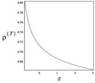
Figure 1: Variation of the effective energy density versus the redshift for $f(T)=T+f_{0}(-T)^{p}$.

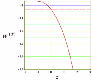
Figure 2: Variation of effective equation of state parameter versus the redshift for $f(T)=T+f_{0}(-T)^{p}$ ,where the dash lines represent $\omega^{(T)}_{0}=-1.03$

3.2 Phantom-like Effect with $f(T)=T+\xi T(1-e^{\frac{\alpha T_{0}}{T}})$

In this model $\alpha$ is an independent parameter and $T_{0}=T(z=0)$ is the current value of the torsion scaler. In the limit $\alpha\rightarrow 0$, this model recovers the $\Lambda CDM$ model[34]. Also, by using the modified Friedmann equation, we find

$$\xi=-\frac{1-\Omega_{m0}}{1-(1-2\alpha)e^{\alpha}}\,.$$ (30)

In this model, if $\alpha>0$ the universe has a phantom phase (with $\omega<-1$) and if $\alpha<0$ it has a quintessence phase (with $\omega>-1$) [48]. For this form of $f(T)$ function we obtain

$$F(T)=\xi T(1-e^{\frac{\alpha T_{0}}{T}})\,,$$ (31)

$$F_{T}=\frac{\xi\alpha T_{0}}{T}e^{\frac{\alpha T_{0}}{T}}+\xi(1-e^{\frac{\alpha T_{0}}{T}})\,,$$ (32)

and

$$F_{TT}=-\frac{\alpha^{2}T_{0}^{2}\xi}{T^{3}}e^{\frac{\alpha T_{0}}{T}}\,.$$ (33)

once again, using equations (20) and (21) we acquire $\rho^{(T)}$ and $\omega^{(T)}$ in the present model as follows

$$\rho^{(T)}=\frac{2\alpha\xi T_{0}e^{\frac{\alpha T_{0}}{T}}+T\xi(1-e^{\frac{\alpha T_{0}}{T}})}{16\pi G}\,,$$ (34)

and

$$\omega^{(T)}=-1+\frac{\Big{(}T\xi(e^{\frac{\alpha T_{0}}{T}}-1)-2\xi\alpha T_{0}e^{\frac{\alpha T_{0}}{T}}-T\Big{)}\Big{(}\xi-\xi e^{\frac{\alpha T_{0}}{T}}(1-\frac{\alpha T_{0}}{T}+\frac{2\alpha^{2}T_{0}^{2}}{T^{2}})\Big{)}}{\Big{(}T\xi(e^{\frac{\alpha T_{0}}{T}}-1)-2\xi\alpha T_{0}e^{\frac{\alpha T_{0}}{T}}\Big{)}\Big{(}\xi-\xi e^{\frac{\alpha T_{0}}{T}}(1-\frac{\alpha T_{0}}{T}+\frac{2\alpha^{2}T_{0}^{2}}{T^{2}})+1\Big{)}}\,,$$ (35)

respectively. We try to see possible realization of the effective phantom-like behavior in this model by numerical treatment of these quantities. We investigated the the behavior of $\rho^{(T)}$ and $\omega^{(T)}$ versus the redshift $z$ for different choices of the model parameter $\alpha$. Our analysis shows that the phase of expansion of the universe (according to the values of $\omega$) depends on the sign of the parameter $\alpha$. We find that $\alpha=0.07$ is the acceptable value for realization of an effective phantom-like behavior in this model. By using the equations (34) and (35), the evolution of $\rho^{(T)}$ and $\omega^{(T)}$ versus the redshift are shown respectively in figures 3 and 4. Figure 3 shows an increasing (positively growing) energy density with the cosmic time (inverse of the redshift). In figure 4, as we can see with the proper selection of parameters, this model can display $\omega^{(T)}=-1.03$ for present time. Also figure 4 shows that the effective equation of state stays always less than $-1$ in this model. Therefore, we note that in this model the crossing of the phantom divide could not occur and the universe evermore is in the phantom phase. Similar to the previous case, this behavior is not in the favor of the observational data that shows transition from the quintessence phase to the phantom phase. Therefore, we can conclude that the present model is not observationally viable.

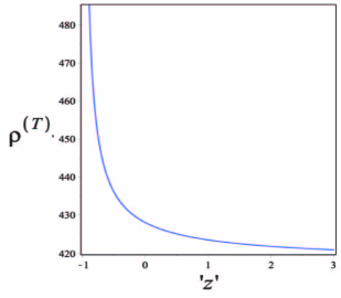
Figure 3: Variation of the effective energy density versus the redshift for $f(T)=T+\xi T(1-e^{\frac{\alpha T_{0}}{T}})$.

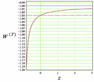
Figure 4: Variation of effective equation of state parameter versus the redshift for $f(T)=T+\xi T(1-e^{\frac{\alpha T_{0}}{T}})$, where the dash lines represent $\omega^{(T)}_{0}=-1.03$.

3.3 Phantom-like Effect with $f(T)=T+n\Big{(}T-Te^{(\frac{\beta T_{0}}{T})}+(-T)^{\beta}\Big{)}$

The above two models have been used in the literatures for a variety of purposes. Possible transition to the phantom phase of the cosmic expansion has been treated with the mentioned $f(T)$ models in a context a little different from our approach. Here, and for the sake of more novelty of the treatment, we consider a combined model that contains a relatively more general $f(T)$ function. This approach is introduced in Ref. [48]. The number of free parameters here are more than the previous cases. Usually with a wider parameter space one expects to encounter more fine-tuning of the parameter to have cosmologically viable solutions. But, in the same time it is more easier, in principle, to find some subspaces of the model parameter space to fulfill the required expectation. For the sake of simplicity,we have taken $\xi=f_{0}\equiv n$ and $p=\alpha\equiv\beta$ .Here $\beta$ and $n$ are two parameters of model that only $\beta$ is free parameter because $n$ can be obtained as

$$n=-\frac{\Omega_{m0}-1}{((1-2\beta)6H_{0})^{2\beta-2}+\Big{(}1-(1-2\beta)e^{\beta}\Big{)}}\,.$$ (36)

Also for this combined model, we can acquire

$$F(T)=n\Big{(}T-Te^{(\frac{\beta T_{0}}{T})}+(-T)^{\beta}\Big{)}\,,$$ (37)

$$F_{T}=\frac{n\beta T_{0}}{T}e^{\frac{\beta T_{0}}{T}}+n(1-e^{\frac{\beta T_{0}}{T}})-n\beta(-T)^{\beta-1}\,,$$ (38)

and

$$F_{TT}=-\frac{n\beta^{2}T_{0}^{2}}{T^{3}}e^{\frac{\beta T_{0}}{T}}+n\beta(\beta-1)(-T)^{p-2}\,.$$ (39)

Similar to the former two models, by using equations (20) and (21) we obtain the effective density and equation of state parameter for this model respectively as follows

$$\rho^{(T)}=\frac{n\Big{(}(-T)^{\beta}(2\beta-1)+T+e^{\frac{\beta T_{0}}{T}}(2\beta T_{0}-T)\Big{)}}{16\pi G}\,,$$ (40)

and

$$\omega^{(T)}=-1+\Theta\Upsilon\,,$$ (41)

where we have defined

$$\Theta\equiv\frac{\Big{(}n(-T)^{\beta}(1-2\beta)+e^{\frac{\beta T_{0}}{T}}(Tn-2n\beta T_{0})-T(1+n)\Big{)}}{\Big{(}(-T)^{n}(1-2\beta)+e^{\frac{\beta T_{0}}{T}}(T-2\beta T_{0})-T\Big{)}}$$ (42)

and

$$\Upsilon\equiv\frac{\Big{(}1+(\frac{\beta T_{0}}{T}-\frac{2\beta^{2}T_{0}^{2}}{T^{2}}-1)e^{\frac{\beta T_{0}}{T}}+(1-2\beta)\beta(-T)^{\beta-1}\Big{)}}{\Big{(}1+n(\frac{\beta T_{0}}{T}-\frac{2\beta^{2}T_{0}^{2}}{T^{2}}-1)e^{\frac{\beta T_{0}}{T}}+n+n\beta(1-2\beta)(-T)^{\beta-1}\Big{)}}\,.$$ (43)

Finally, to investigate the possible realization of the phantom-like behavior in this combined model,by using equations (40) and (41), we plot $\rho^{(T)}$ and $\omega^{(T)}$ versus the redshift for different values of $\beta$. We observe that the two conditions for effective phantom mimicry a)the effective energy density must be positive and growing with time b) the equation of state parameter should be less than $-1$, are satisfied if $\beta=0.2$. This typical behavior of $\rho_{T}$ and $\omega_{T}$ versus the redshift are shown in figures 5 and 6 respectively. We note that unlike the previous two cases, this model is strictly in the favor of the observational data. As is seen from figure 6, it is obvious that the effective equation of state parameter can cross the $\omega=-1$ line at $0.5<z_{cross}<1$ and amount $\omega_{T}$ for Current time $z=0$ is consistent with the resent observational data. It means that universe evolves from quintessence-like phase towards the phantom-like phase. We can conclude that this model is capable of realizing a suitable dynamical mechanism for getting the present time cosmic acceleration and transition to a phantom-like stage in a fascinating manner. Consequently, this model is more cosmologically viable than the previous two models.

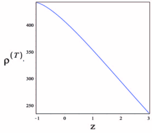
Figure 5: Variation of the effective energy density versus the redshift for $f(T)=T+n\Big{(}T-Te^{(\frac{\beta T_{0}}{T})}+(-T)^{\beta}\Big{)}$.

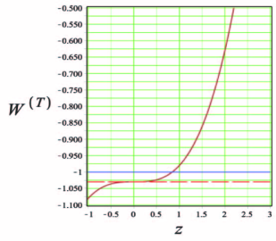
Figure 6: Variation of effective equation of state parameter versus the redshift for $f(T)=T+n\Big{(}T-Te^{(\frac{\beta T_{0}}{T})}+(-T)^{\beta}\Big{)}$, where the dash lines represent $\omega^{(T)}_{0}=-1.03$.

4 conclusion

In this paper we have investigated possible realization of an effective phantom behavior in some viable $f(T)$ gravity models. With effective phantom-like behavior we mean an effective energy density that should be positive and growing positively with time and also, the equation of state parameter should be less than $-1$. We have chosen three different models of $f(T)$ gravity that two of them are reliable based on previous studies and Our third model is a combined model. We have shown that model with $f(T)=T+f_{0}(-T)^{p}$ realizes an effective phantom-like behavior if $p=0.028$.As is shown in figure 2, we obtained the effective equation of state parameter for present time about $\omega^{(T)}_{0}=-1.03$ that this amount is acceptable according to the recent data from Planck2018. But, this model evolves from effective phantom-like phase towards the effective quintessence-like phase in future. Thus, this model is not in the complete favor of observation, since observation shows transition from quintessence-like to phantom-like phase. We have presented another $f(T)$ model, which is $f(T)=T+\xi T(1-e^{\frac{\alpha T_{0}}{T}})$. This $f(T)$ model realizes an effective phantom like behavior if $\alpha=0.07$. Although, $\omega^{(T)}_{0}$ is obtained a acceptable value that is shown in figure 4 ,but this $f(T)$ function is not also in the favor of observation. Since in this model the crossing of the phantom divide could not occur and the universe evermore is in the phantom phase . Finally, we have constructed a $f(T)$ theory by combining the two previous models that it only contains one model parameter $\beta$. This model realizes an effective phantom-like behavior if $\beta=0.2$. Unlike the previous two models, this model is cosmologically more viable, since the equation of state parameter in this model evolves from effective quintessence-like phase towards an effective phantom-like phase.As is shown in figure 6, it is obvious that $\omega^{(T)}$ can cross the $\omega=-1$ line at $0.5<z_{cross}<1$ and amount $\omega^{(T)}_{0}$ is consistent with the resent observational data. Therefore, this combined model is in agreement with the observational data.

Acknowledgment

It is a pleasure to thank Prof. Kourosh Nozari for helpful discussions and valuable comments.

Data Availability

The data used to support the findings of this study are included within the article.

References

- [1] S. Perlmutter et al, ”Measurements of Omega and Lambda from 42 High-Redshift Supernovae” , Astrophysical Journal, vol.517, pp.565-586, 1999.
- [2] A. G. Riess et al,”Type Ia Supernova Discoveries at From the Hubble Space Telescope Evidence for Past Deceleration and Constraints on Dark Energy Evolution”, Astrophysical Journal,vol.607, pp.665-687, 2004.
- [3] G.Hinshaw et al, ”Three-Year Wilkinson Microwave Anisotropy Probe (WMAP) Observations: Temperature Analysis”, The Astrophysical Journal Supplement Series, 2007.
- [4] D. Hinshaw et al, ”Nine-Year Wilkinson Microwave Anisotropy Probe (WMAP) Observations: Cosmological Parameter Results”,Astrophysics:Cosmology and Nongalactic Astrophysics,2012.
- [5] C. Bennett et al, ”Nine-Year Wilkinson Microwave Anisotropy Probe (WMAP) Observations: Final Maps and Results”,Astrophysics:Cosmology and Nongalactic Astrophysics,2012.
- [6] M. Tegmark et al,”Cosmological parameters from SDSS and WMAP”,Physical Review D: particles, fields, gravitation, and cosmology,Article ID 103501,2004.
- [7] S.P. Boughn and R.G. Crittenden,”A Detection of the Integrated Sachs-Wolfe Effect”,Nature,2004.
- [8] P. A. R. Ade et al,”Planck 2013 results. XVI. Cosmological parameters”,Astrophysics : Cosmology and Nongalactic Astrophysics, 2013.
- [9] N. Aghanim et al, ”Planck 2018 results. VI. Cosmological parameters”,Astrophysics : Cosmology and Nongalactic Astrophysics,2018.
- [10] J. Weller, ”Bubbles from dark energy?” ,Astrophysics,2000.
- [11] E. J. Copeland, M. Sami and S. Tsujikawa,”Dynamics of dark energy”,High Energy Physics - Theory,2006.
- [12] Y.-F. Cai, E. N. Saridakis, M. R. Setare and J.-Q. Xia, ”Quintom Cosmology: Theoretical implications and observations”, High Energy Physics - Theory,2009.
- [13] A. De Felice and S. Tsujikawa,”f(R) theories”,General Relativity and Quantum Cosmology,2010.
- [14] S. Nojiri and S. D. Odintsov, ”Unified cosmic history in modified gravity: from F(R) theory to Lorentz non-invariant models”,General Relativity and Quantum Cosmology,2011.
- [15] S. Nojiri and S. D. Odintsov, ”Modified Gauss-Bonnet theory as gravitational alternative for dark energy”,Physics Letters B,vol.631,2005.
- [16] A. De Felice and S. Tsujikawa,”Construction of cosmologically viable f(G) dark energy models”,Physics Letters B,vol.675,2009.
- [17] C. de Rham , ”Massive Gravity”,Living Review. Relativity,vol.17,no.7,2014.
- [18] N. Deruelle and L. Farina-Busto, ”The Lovelock Gravitational Field Equations in Cosmology”, Physical Review D , vol.41, no.3696, 1990.
- [19] P. Horava ,”Membranes at Quantum Criticality”,High Energy Physics - Theory,vol. 0903, no.020, 2009.
- [20] K. Nozari , ”DGP Cosmology with a Non-Minimally Coupled Scalar Field on the Brane”,Journal of Casmology and Astroparticle Physics,2007.
- [21] K. Hayashi and T. Shirafuji, ”New general relativity” , Physical Review D ,vol.19,no.3524,1979.
- [22] A. Unzicker and T. Case, ”Translation of Einstein’s Attempt of a Unified Field Theory with Teleparallelism”, History and Philosophy of Physics, 2005.
- [23] G. Y. Chee, Y. Zhang and Y. Guo,”Gravitational energy-momentum and the Hamiltonian formulation of the teleparallel gravity”,General Relativity and Quantum Cosmology, 2001.
- [24] R. Aldrovandi and J. G. Pereira, ”Teleparallel Gravity: An Introduction”, Springer,2013.
- [25] J. W. Maluf,”The teleparallel equivalent of general relativity”,General Relativity and Quantum Cosmology,2013.
- [26] G. R. Bengochea and R. Ferraro, ”Dark torsion as the cosmic speed-up”, Physical Review D ,vol.79, no.124019,2009.
- [27] P. Wu and H. Yu,”The dynamical behavior of f(T) theory”, Physics Letters B ,vol.692, pp.176-179,2010.
- [28] J. B. Dent, S. Dutta and E. N. Saridakis,”f(T) gravity mimicking dynamical dark energy Background and perturbation analysis”,Astrophysics : Cosmology and Nongalactic Astrophysics, 2011.
- [29] S. M. Carroll,”The Cosmological Constant”, Living Reviews in Relativity,vol. 4, no. 1, 2001.
- [30] T. Padmanabhan,”Cosmological Constant - the Weight of the Vacuum”, Physics Reports, vol.380, no. 235, 2003.
- [31] K. Nozari, R. Shojaee and S. Karimzadeh,”interpretation of Rotation Curves of Spiral Galaxies in Modified Teleparallel Gravity” ,Communications in Theoretical Physics , 2013.
- [32] A. Behboodi, S. Akhshabi and K. Nozari,”Braneworld setup and embedding in teleparallel gravity”, Physics Letters B,2014.
- [33] F. Kiani and K. Nozari ,”Energy conditions in gravity and compatibility with a stable de Sitter solution”,Physics Letters B, 2014 .
- [34] Y. -F. Cai, S. Capozziello, M. D. Laurentis and E. N. Saridakis,”f(T) teleparallel gravity and cosmology”,Review for Reports on Progress in Physics,vol.79, no.04, 2016.
- [35] R. C. Nunes,”Structure formation in f(T) gravity and a solution for H0 tension”,Journal of Casmology and Astroparticle Physics,vol.05, no.052, 2018.
- [36] G. G. L. Nashed and E. N. Saridakis,”Rotating AdS black holes in Maxwell-f(T)gravity”,High Energy Physics - Theory, 2018.
- [37] U. Debnath, ”Charge Gravastars in f(T) Modified Gravity”, General Relativity and Quantum Cosmology , 2019.
- [38] R. C. Nunes, S. Pan and E. N. Saridakis,”New observational constraints on f(T) gravity from cosmic chronometers”,Journal of Casmology and Astroparticle Physics,vol.1608, no.08,2016.
- [39] R. C. Nunes, A. Bonilla, S. Pan and E. N. Saridakis,”Observational Constraints on f(T) gravity from varying fundamental constants”,The Eropean Physical Journal C ,vol.77, no.230, 2017.
- [40] L. P. Chimento, R. Lazkoz, R. Maartens and I. Quiros,”Crossing the phantom divide without phantom matter”,Journal of Casmology and Astroparticle Physics, vol.609, no.004,2006.
- [41] V. Sahni and Y. Shtanov,”Braneworld models of dark energy”,Journal of Cosmology and Astroparticle Physics,2003.
- [42] V. Sahni,”Cosmological Surprises from Braneworld models of Dark Energy”,General relativity and Gravitation,2005.
- [43] A. Lue and G. D. Starkman,”How a brane cosmological constant can trick us into thinking that w ¡ -1”,Physical Review D,vol.70, no.101501, 2004.
- [44] K. Nozari and M. Pourghasemi,”Crossing the Phantom Divide Line in a DGP-Inspired -Gravity”,Journal of Cosmology and Astroparticle Physics,vol.10, no.044, 2008.
- [45] K. Nozari and T. Azizi, ”Phantom-Like Effects on Warped DGP Brane”,Communications in Theoretical Physics,2010.
- [46] K. Nozari and N. Alipour,”Phantom Mimicry on the Normal Branch of a DGP-inspired Braneworld Scenario with Curvature Effect”,General Relativity and Quantum Cosmology,2009.
- [47] K. Nozari and T. Azizi,”Phantom-Like in Gravity”,Physics Letters B,vol.608, no.205, 2009.
- [48] K. Bamba, C. -Q. Geng, C. -C Lee and L. -W. Luo,”Equation of state for dark energy in f(T) gravity”,Journal of Cosmology and Astroparticle Physics,2011.
- [49] R. -J. Yang,”New types of f(T) gravity”,The Eropean Physical Journal C ,2011.
- [50] P. Wu and H. Yu,”Observational constraints on f(T) theory”, Physics Letters B, 2010.
- [51] J. B. Dent, S. Dutta and E. N. Saridakis,”f(T) gravity mimicking dynamical dark energy. Background and perturbation analysis”,Journal of Cosmology and Astroparticle Physics,2010.
- [52] C. -Q. Geng, C. -C. Lee, E. N. Saridakis and Y. -P. Wu,”Teleparallel Dark Energy”,Physics Letters B, vol.704,pp.384-387, 2011.
- [53] A. Behboodi, S. Akhshabi and K. Nozari,”Matter stability in modified teleparallel gravity”,Physics Letters B, vol.718, no.30, 2012.
- [54] K. Hayashi and T. Shirafuji,”New general relativity”,Physical Review D ,1979.
- [55] A. Paliathanasis, J. D. Barrow and P.G.L. Leach,”Cosmological Solutions of f(T) Gravity”,Physical Review D ,vol.94, no.023525, 2016.
- [56] Y. -Fu. Cai, T. Qiu, Y. -S. Piao, M. Li and X. Zhang,Journal of Cosmology and Astroparticle Physics ,vol.0710,no.071,2007.
- [57] S. Nesseris, S. Basilakos, E. N. Saridakis, L. Perivolaropoulos,”Viable f(T) models are practically indistinguishable from LCDM”,Physical Review D ,2013.