Using discrete Darboux polynomials to detect and determine preserved measures and integrals of rational maps

Abstract

In this Letter we propose a systematic approach for detecting and calculating preserved measures and integrals of a rational map. The approach is based on the use of cofactors and Discrete Darboux Polynomials and relies on the use of symbolic algebra tools. Given sufficient computing power, all rational preserved integrals can be found. We show, in two examples, how to use this method to detect and determine preserved measures and integrals of the considered rational maps.

1 Introduction

The search for preserved measures and integrals of ordinary differential equations (ODEs) has been at the forefront of mathematical physics since the time of Galileo and Newton.

In this Letter our aim will be to develop an analogous theory for the (arguably more general) discrete-time case. This will lead to essentially linear algorithms for detecting and determining preserved measures and first and second integrals of (discrete) rational maps (both integrable and non-integrable).

But before we consider the discrete case, let us look at the continuous case, i.e. ODEs.

Consider two polynomials $P_{1}$ and $P_{2}$:

$$P_{1}(\mathbf{x}) = \sum a_{i_{1},\dots,i_{n}}x_{1}^{i_{1}}\dots x_{n}^{i_{n}}$$

$$P_{2}(\mathbf{x}) = \sum b_{i_{1},\dots,i_{n}}x_{1}^{i_{1}}\dots x_{n}^{i_{n}}.$$

Then $I:=P_{1}/P_{2}$ is a rational integral of the ODE $\frac{d\mathbf{x}}{dt}=f(\mathbf{x})$ if

$$\dot{P_{1}}P_{2}-P_{1}\dot{P_{2}}=0$$

along solutions of the ODE. Here $\dot{}$ denotes $\frac{d}{dt}$.

For a polynomial ODE, the problem of finding $P_{1}$ and $P_{2}$, as posed, is bilinear in the parameters $a_{i_{1},\dots,i_{n}}$ and $b_{i_{1},\dots,i_{n}}$.

1.1 Darboux polynomials (ODE case)

Let $P(\mathbf{x})$ and $C(\mathbf{x})$ be polynomials.

Then $P(\mathbf{x})$ is called a Darboux polynomial of the polynomial ODE $\frac{d\mathbf{x}}{dt}=f(\mathbf{x})$, if

$$\dot{P}(\mathbf{x})=C(\mathbf{x})P(\mathbf{x}).$$

Here $C(\mathbf{x})$ is called the co-factor of $P$.

Note that $P(\mathbf{\mathbf{x}}(0))=0$ implies $P(\mathbf{x}(t))=0$ for all $t$. Hence the set $P(\mathbf{x})=0$ is an invariant set in phase space.

Consider two Darboux polynomials with the same co-factor $C$:

$$\begin{array}[]{c}\dot{P}_{1}=CP_{1}\\ \dot{P}_{2}=CP_{2}\end{array}\Rightarrow\frac{d}{dt}\left(\frac{P_{1}}{P_{2}}\right)=\frac{\dot{P}_{1}P_{2}-P_{1}\dot{P}_{2}}{P_{2}^{2}}=\frac{CP_{1}P_{2}-P_{1}CP_{2}}{P_{2}^{2}}=0,$$ (1)

i.e. the ratio of two Darboux polynomials with the same cofactor is a rational integral. (The converse is also true).

However, finding $C$, $P_{1}$ and $P_{2}$ involves one bilinear problem, plus one linear problem. (Nevertheless, this approach can still be useful).

More generally,

$$\begin{array}[]{c}\dot{P}_{1}=C_{1}P_{1}\\ \dot{P}_{2}=C_{2}P_{2}\end{array}\Rightarrow\frac{d}{dt}(P_{1}P_{2})=\dot{P}_{1}P_{2}+P_{1}\dot{P}_{2}=(C_{1}+C_{2})P_{1}P_{2}.$$ (2)

A very nice introduction to Darboux polynomials for ODEs was given by Goriely [6]. Note that Darboux polynomials were studied by Darboux, Poincaré, Painlevé and others [6], and are also known by several other names, including “second integrals” and “weak integrals”.

1.2 Discrete Darboux Polynomials (mapping case)

Instead of polynomial ODEs $\frac{d\mathbf{x}}{dt}=f(\mathbf{x})$, we now consider rational maps $\mathbf{x}_{n+1}=\phi(\mathbf{x}_{n})$ (cf [4, 5]).

Then we define $P(\mathbf{x})$ to be a Discrete Darboux Polynomial of the rational map $\mathbf{x}_{n+1}=\phi(\mathbf{x}_{n})$ if

$$P(\mathbf{x}_{n+1})=C(\mathbf{x}_{n})P(\mathbf{x}_{n}),$$

where the co-factor $C$ is now a rational function whose form will be presented in §1.3.

We use the shorthand notation

$$P^{\prime}=CP$$

Note that, similarly to the continuous case, $P(\mathbf{x})=0$ is an invariant set in phase space.

Now consider again two Discrete Darboux Polynomials $P_{1}$ and $P_{2}$ with the same co-factor $C$:

$$\begin{array}[]{c}P_{1}^{\prime}=CP_{1}\\ P_{2}^{\prime}=CP_{2}\end{array}\Rightarrow\frac{P_{1}^{\prime}}{P_{2}^{\prime}}=\frac{P_{1}}{P_{2}},$$

i.e. the ratio of the two Discrete Darboux Polynomials with the same co-factors is again an integral (and the converse is also true).

More generally

$$\begin{array}[]{c}P_{1}^{\prime}=C_{1}P_{1}\\ P_{2}^{\prime}=C_{2}P_{2}\end{array}\Rightarrow(P_{1}P_{2})^{\prime}=C_{1}C_{2}(P_{1}P_{2})$$

How is all this going to help us find integrals of a given map?

The answer comes in two parts:

1. In the discrete case we use a non-trivial ansatz for the co-factors $C(\mathbf{x})$. This ansatz works in all examples we have tried so far.

2. In the discrete case the co-factor of the product is the product of the co-factors.
   In the continuous case the co-factor of the product is the sum of the co-factors.

The latter point is crucial: It means that in the discrete case we can use the fact that the factorization of the co-factor $C$ is unique. By contrast, in the ODE case we have addition, where splitting into summands is not unique.

1.3 Ansatz

Ansatz: The co-factors we use are of the form

$$C(\mathbf{x})=\frac{1}{D^{l}(\mathbf{x})}\prod_{i}K_{i}^{a_{i}}(\mathbf{x})$$

where $D(\mathbf{x})$ is the common denominator of the map, and the $K_{i}(\mathbf{x})$ are factors of the numerator of the Jacobian determinant $J(\mathbf{x})$ of the map:

$$J(\mathbf{x})=\frac{1}{D^{m}(\mathbf{x})}\prod_{i}K_{i}^{b_{i}}(\mathbf{x})$$

Comments:

1. There is a finite number of these co-factors up to a certain degree.

2. For each of this finite number of co-factors, we only need to solve a linear problem (up to a chosen degree).

3. If $C(\mathbf{x})=J(\mathbf{x})$, the corresponding Darboux polynomials are (inverse) densities of preserved measures.

2 Determining preserved measures and first and second integrals of rational maps

In this section we study the following two-dimensional ODE as an example:

$$\frac{dx}{dt} = x(x+6y-3)$$ (3)

$$\frac{dy}{dt} = y(-3y-2x+3)$$

The Kahan-Hirota-Kimura (KHK) discretization of (3) reads (cf [2, 3, 8, 9, 10, 11, 14])

$$x^{\prime} = \frac{x(1+h(x+6y-3)+\frac{h^{2}}{4}(9-6x))}{D(x)}$$ (4)

$$y^{\prime} = \frac{y(1+h(3-2x-3y)+\frac{9h^{2}}{4}(1-2y))}{D(x)}$$

where the common denominator $D(\mathbf{x})$ of the map is given by

$$D(\mathbf{x}):=1-\frac{h^{2}}{4}(9-12x-36y+4x^{2}+12xy+36y^{2})$$ (5)

The Jacobian determinant $J(\mathbf{x})$ of the mapping (4) is

$$J(\mathbf{x})=\frac{K_{1}(\mathbf{x})K_{2}(\mathbf{x})K_{3}(\mathbf{x})}{D^{3}(\mathbf{x})}$$ (6)

where

$$K_{1} = 1+h(x-3y)-\frac{3}{4}h^{2}(3-2x-6y)$$

$$K_{2} = 1+h(x+6y-3)-\frac{3}{4}h^{2}(3-2x)$$ (7)

$$K_{3} = 1+h(3-2x-3y)+\frac{9}{4}h^{2}(1-2y)$$

We have used cofactors $C_{1}=\frac{K_{1}}{D}$, $C_{2}=\frac{K_{2}}{D}$, $C_{3}=\frac{K_{3}}{D}$, $C_{4}=J$ to find the corresponding Discrete Darboux Polynomials for the map (4):

$$p_{1,1}= x+3y-3$$

$$p_{2,1}= x$$

$$p_{3,1}= y$$

$$p_{4,1}= xy(x+3y-3)$$

$$p_{4,2}= 1-\frac{h^{2}}{4}(9-12x-36y+4x^{2}+12xy+36y^{2})$$

Here $p_{i,j}$ denotes the $j^{th}$ Darboux polynomial corresponding to the cofactor $C_{i}$.

A phase plot for the map (4), clearly exhibiting the linear Darboux polynomials $p_{1,1}$, $p_{2,1}$, and $p_{3,1}$, is given in Figure 1.

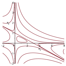
Figure 1: Phase plot for map (4) and for $h=\frac{1}{17}$

It follows that the map (4) preserves the integral

$$\tilde{I}(\mathbf{x})=\frac{xy(x+3y-3)}{1-\frac{h^{2}}{4}(9-12x-36y+4x^{2}+12xy+36y^{2})}$$ (8)

and the measure

$$\frac{dxdy}{1-\frac{h^{2}}{4}(9-12x-36y+4x^{2}+12xy+36y^{2})}$$ (9)

Taking the continuum limit $h\rightarrow 0$, we obtain the cofactors $\tilde{C}_{1}=x-3y$, $\tilde{C}_{2}=x+6y-3$, $\tilde{C}_{3}=3-2x-3y$, $\tilde{C}_{4}=0$, and the corresponding Darboux polynomials

$$p_{1,1}= x+3y-3$$

$$p_{2,1}= x$$

$$p_{3,1}= y$$

$$p_{4,1}= xy(x+3y-3)$$

$$p_{4,2}= 1$$

It follows that the ODE (3) preserves the integral

$$I(\mathbf{x})=xy(x+3y-3)$$ (10)

and the measure

$$dxdy.$$ (11)

It thus turns out that our original ODE (3) is Hamiltonian, with $H(x)=xy(x+3y-3)$.

Interpreted conversely, one can say that the KHK discretization (4) preserves the three affine Darboux polynomials of the ODE (3), as well as the modified integral (8) and the modified density (9). These results are no coincidences.

Indeed, the preservation of the three affine Darboux polynomials is the consequence of the following theorem (whose proof we will present elsewhere).

Theorem 1.

The KHK discretization preserves all affine Darboux polynomials of a given quadratic ODE.

Theorem 1 is a very significant step towards the full resolution of the open problem posed in 2002 in [12]: ‘How does one preserve more than $n-1$ integrals and weak integrals (of an $n$-dimensional vector field)?’

The preservation of the modified integral and measure is an example of a general result in [2] giving a modified integral for all systems with a cubic Hamiltonian in any dimension.

3 Detecting preserved measures and first and second integrals of rational maps

In this section we consider the following three-dimensional ODE as an example:

$$\frac{dx}{dt} = x(y-\mu z)$$

$$\frac{dy}{dt} = y(\lambda z-x)$$ (12)

$$\frac{dz}{dt} = z(\mu x-\lambda y),$$

where $\lambda$ and $\mu$ are arbitrary parameters.

Applying the Kahan-Hirota-Kimura discretization to (3), we obtain

$$\frac{x^{\prime}-x}{h} = \frac{x^{\prime}(y-\mu z)+x(y^{\prime}-\mu z^{\prime})}{2}$$

$$\frac{y^{\prime}-y}{h} = \frac{y^{\prime}(\lambda z-x)+y(\lambda z^{\prime}-x^{\prime})}{2}$$ (13)

$$\frac{z^{\prime}-z}{h} = \frac{z^{\prime}(\mu x-\lambda y)+z(\mu x^{\prime}-\lambda y^{\prime})}{2}.$$

Solving equation (3) for $x^{\prime}$, $y^{\prime}$, and $z^{\prime}$ we obtain the (rational) Kahan map discretizing (3). Using the Jacobian determinant $J(\mathbf{x})$ of the Kahan map as cofactor, our algorithm finds that for all $(\mu,\lambda)$, the map preserves the measure $\frac{dxdydz}{xyz}$ and the first integral $x+y+z$.

Moreover, the algorithm also detects the following special values of the parameters $(\mu,\lambda)$ where the map preserves an additional integral, and outputs the formula for the integral (cf. Table 1).

Table 1: Integrable parameter values and corresponding functionally independent additional first integrals detected by our algorithm.

$(\mu,\lambda)$	additional first integral
$(-1,0)$	$y/z$
$(1,0)$	$yz/(1-\frac{h^{2}}{4}x^{2})$
$(0,1)$	$xz/(1-\frac{h^{2}}{4}y^{2})$
$(0,-1)$	$z/x$
$(1,1)$	$xyz/(1-\frac{h^{2}}{4}(x^{2}+y^{2}+z^{2}-2xy-2xz-2yz))$
$(1,-1)$	$x/yz$
$(-1,-1)$	$z/xy$
$(-1,1)$	$y/xz$

4 Concluding remarks

In this Letter we have presented a method for detecting and determining first and second integrals of rational maps. There are in the literature several other methods for determining first and second integrals of discrete systems, cf. [4, 5, 13, 16] and references therein. There are also in the literature several other methods for detecting first and second integrals of discrete systems, cf. [1, 8, 15] and references therein.

However, to our knowledge none of the above combine all the following properties of the method presented in this Letter:

1. It is algorithmic, and requires no other input than the rational map in question. At heart the algorithm is linear and, to some extent apart from birationality, requires no knowledge about the map (such as symplecticity, measure preservation, time-reversal symmetry, integrability, Lax pairs, etc) on the part of the user.

2. Up to a certain prescribed degree, it determines and outputs all:

   1. rational first integrals

   2. polynomial second integrals

   3. preserved measures of the form $P(x)dx$ or $\frac{dx}{P(x)}$, where $P$ is a polynomial.

3. It can detect special parameter values where additional preserved first and/or second integrals and/or measures exist, and output those integrals and measures.

4. It works for both integrable and non-integrable cases.

5. It allows one to take the continuum limit, if appropriate.

References

• [1] Abarenkova N, AnglΓ¨s d’Auriac J-Ch, Boukraa S and Maillard J-M 2000, Real topological entropy versus metric entropy for birational measure-preserving transformations, Physica D144 387–433
• [2] Celledoni E, McLachlan RI, Owren B and Quispel GRW 2013, Geometric properties of Kahan’s method J. Phys. A 46 12 pp. 025201
• [3] Celledoni E, McLachlan RI, McLaren DI, Owren B and Quispel GRW 2014, Integrability properties of Kahan’s method. J. Phys. A 47 20 pp. 365202
• [4] Falqui G and Viallet C-M 1993, Singularity, complexity, and quasi-integrability of rational mappings, Comm. Math. Phys. A 154, 111–125
• [5] Gasull A and Manosa V 2010, A Darboux-type theory of integrability for discrete dynamical systems, Journal of Difference Equations and Applications 8 1171-1191
• [6] Goriely A 2001, Integrability and Nonintegrability of Dynamical Systems, World Scientific, Singapore, section 2.5
• [7] Halburd RG and Korhonen RJ 2017, Three approaches to detecting discrete integrability, ArXiv: 1704.07927
• [8] Hirota R and Kimura K 2000, Discretization of the Euler top, J. Phys. Soc. Jap. 69 627–630.
• [9] Hone A N W and Petrera M 2009, Three dimensional discrete systems of Hirota-Kimura type and deformed Lie-Poisson algebras, Journal of Geometric mechanics 1 No.1 55–85.
• [10] Kimura K and Hirota R, 2000, Discretization of the Lagrange top. J. Phys. Soc. Japan 69 3193–3199.
• [11] Kahan W 1993, Unconventional numerical methods for trajectory calculations, Unpublished lecture notes.
• [12] McLachlan RI and Quispel GRW 2002, Splitting Methods, Acta Numerica 11 341–434, section 6.1.
• [13] Papageorgiou VG, Nijhoff FW and Capel HW 1990, Integrable mappings and nonlinear integrable lattice equations, Phys Lett 147A 106–114
• [14] Petrera M, Pfadler A and Suris YB 2011, On integrability of Hirota–Kimura type discretizations, Regular and Chaotic Dynamics 16 245–289.
• [15] JAG Roberts and F Vivaldi, 2003, Arithmetical method to detect integrability in maps, Phys Rev Lett 90(3) 034102.
• [16] Tran DT, van der Kamp PH and Quispel GRW 2009, Closed-form expressions for integrals of travelling wave reductions of integrable lattice equations, J Phys A 42 225201