An analytic approach to the Riemann hypothesis

Abstract

In this work we consider an equation for the Riemann $\zeta$-function in the critical half-strip

$${\mathbb{S}}^{+}=\left\{s=x+iy\in{\mathbb{C}}\;:\;{\frac{1}{2}<x<1},\;{y>0}\right\}.$$

With the help of this equation we prove that finding non-trivial zeros of the Riemann $\zeta$-function outside the critical line ${\rm Re}(s)={1\over 2}$ would be equivalent to the existence of complex numbers $s=x+iy\in{\mathbb{S}}^{+}$ for which

$$\sum_{k=1}^{\infty}(-1)^{k+1}{1\over\zeta(2x)}\sum_{n=1}^{\infty}{\cos\left[y\log\left(1+{k\over n}\right)\right]\over n^{2x}\left(1+{k\over n}\right)^{x}}={1\over 2}.$$

Such a condition is studied, and the attempt of proving the Riemann hypothesis is found to involve also the functional equation

$$\chi_{n}(t)=-\chi_{n}\left(t+{1\over n}\right),$$

where $t$ is a real variable $\geq 1$, and $n$ is any natural number. The limiting behaviour of the solutions $\chi_{n}(t)$ as $t$ approaches $1$ is then studied in detail.

1 Introduction

This introduction, being written for the general reader, describes the early work from Euler’s definition to Riemann’s article. Riemann’s $\zeta$-function is the analytic extension to the whole complex plane of the $\zeta$-function

$${\zeta\left(s\right)=\sum_{n=1}^{\infty}{\frac{1}{{n^{s}}}}},$$ (1.1)

defined by Euler in the region of the complex plane

$${\mathbb{A}}=\left\{{s\in{\mathbb{C}}:{\rm Re}(s)>1}\right\},$$ (1.2)

where it is absolutely convergent. Euler proved that in the region ${\mathbb{A}}$ the $\zeta$-function admits a product representation

$$\zeta(s)=\prod_{p\in{\mathbb{P}}}{\frac{1}{{\left(1-\frac{1}{{p^{s}}}\right)}}}\;{\rm with}\;s\in{\mathbb{A}},\\$$ (1.3)

where ${\mathbb{P}}$ is the set of prime numbers. By virtue of the previous relation Euler was able to prove that in the region ${\mathbb{A}}$ the $\zeta$-function has neither zeros nor poles. Riemann was inspired by this observation to write his masterpiece article in which he looked for an analytical expression for the step-function $\pi\left(x\right)$ which counts the number of primes less than a given number $x\in{\mathbb{R}}^{+}$. During his investigation, he discovered three very important properties of the $\zeta$-function, probably noted but not proved before by Euler. The first was that the $\zeta$-function can be analytically extended to the whole complex plane by virtue of the integral representation

$$\zeta\left(s\right)=\frac{{\Gamma\left({1-s}\right)}}{{2\pi i}}\int\limits_{\gamma}{\frac{{z^{s-1}}}{{\left(e^{z}-1\right)}}dz},$$ (1.4)

where the symbol $\gamma$ indicates a Hankel’s contour of the kind in Fig. 1.

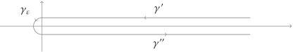
Figure 1: Hankel contour for the integral (1.4).

The second was the discovery of the functional equation

$$\pi^{-{s\over 2}}\Gamma\left(s\over 2\right)\zeta\left(s\right)=\pi^{-\frac{1-s}{2}}\Gamma\left(1-s\over 2\right)\zeta\left(1-s\right),$$ (1.5)

which connects the properties of $\zeta$ in the two half-planes in which the complex plane remains divided by the vertical line

$$r_{1/2}=\left\{s\in{\mathbb{C}}:{\rm Re}(s)=\frac{1}{2}\right\},$$ (1.6)

named the critical line. Riemann pointed out that, by virtue of the functional equation (1.5), upon setting $s_{k}=-2k$ one has $\zeta\left(s_{k}\right)=0$ for any $k\in{\mathbb{N}}$. These zeros, being obtained from the $\sin$ function, are called trivial zeros. Nevertheless, this relation does not assure us that they are all the zeros of the $\zeta$, but it proves only that, if other sets of zeros exist, they must lie in the critical strip

$${\mathbb{S}}=\left\{{s=x+iy\in{\mathbb{C}}:0<x<1}\right\},$$ (1.7)

and that the zeros have to be located symmetrically about the critical line. These zeros are called non-trivial zeros.

Figure 2: The four parts of the critical strip.

As far as their existence is concerned, Hardy [10] proved that, on the Critical Line $r_{1/2}$, there exist infinitely many zeros, but

The Riemann Hypothesis states that there are no non-trivial zeros outside the critical line $r_{1/2}$.

The third result obtained by Riemann was the discovery of a Product Representation in $[{\mathbb{S}}_{\varepsilon}]$ of the function

$$\xi(s)=\frac{{s\left({s-1}\right)}}{2}\pi^{-\frac{s}{2}}\Gamma\left({\frac{s}{2}}\right)\zeta\left(s\right),$$ (1.11)

symmetric, about the Critical Line, of the form

$$\xi(s)=\xi\left(0\right)\prod_{\rho\in{\cal R}}{\left({1-\frac{s}{\rho}}\right)},$$ (1.12)

where ${\cal R}$ is the set of all non-trivial zeros of the $\zeta$-function. By virtue of this representation the Functional Equation (1.5) becomes $\xi\left(s\right)=\xi\left(1-s\right)$. But how are they related with prime numbers? As we said before, the goal of Riemann’s masterpiece article was an analytic expression for the step-function $\pi\left(x\right)$. After having discovered these three properties he proposes the definition of the step function

$$J(x)=\sum_{n=1}^{\infty}{\frac{1}{n}\pi\left({x^{1/n}}\right)},$$

which is, for any $x\in{\mathbb{R}}^{+}$, a finite sum, since by definition $\pi\left(\alpha\right)\equiv 0$ for any $\alpha<2$. Thus, setting $x^{1/n}<2$ we have, for any $n>\frac{\log x}{\log 2}$, that $\pi\left(x^{1/n}\right)\equiv 0$. This sum can be inverted by the Möbius Inversion Formula, obtaining

$$\pi\left(x\right)=\sum_{n=1}^{\left[{\frac{{\log x}}{{\log 2}}}\right]}{\frac{{\mu\left(n\right)}}{n}J\left({x^{1/n}}\right)}.$$ (1.13)

His main result follows by a careful use of (1.3), hence obtaining the analytic expression of $J\left(x\right)$ as (on denoting by ${\rm Li}(x)=\int_{2}^{x}{dt\over(\log t)}$ the logarithmic integral)

$$J\left(x\right)={\rm Li}(x)-\sum\limits_{\rho\in{\cal R}}{{\rm Li}\left({x^{\rho}}\right)}-\log 2+\int\limits_{x}^{\infty}{\frac{{dt}}{{t\left({t^{2}-1}\right)\log t}}}.$$ (1.14)

Upon substituting this expression into (1.13) he obtained the desired result. The dominant term in the Riemann’s main formula (1.14) is

$${\rm Li}\left(x\right)=\frac{x}{{\log x}}-{2\over\log 2}+\int_{2}^{x}{dt\over(\log t)^{2}},$$

which is the asymptotic estimate of the number of primes between 2 and $x$, as stated by the Prime Number Theorem (here $a$ is a positive constant):

$$\left|\pi(x)-{\rm Li}(x)\right|={\rm O}\left(xe^{-a\sqrt{\log(x)}}\right),$$ (1.15)

proved by Hadamard and de La Vallée-Poussin [9, 6]. It was later proved by von Koch [20] that the remainder term in (1.15) is ${\rm O}(\sqrt{x}\log(x))$ if and only if the Riemann hypothesis holds. But the most interesting term of (1.14) is the second, whose sum runs over $\rho\in{\cal R}$. Thus, Riemann understood that his dream to obtain a staircase-function, whose steps were localized on the prime numbers, could be realized if and only if the positions of non-trivial zeros of the Riemann’s $\zeta$-function were known.

During the twentieth century, in the forties, it became clear that the Riemann $\zeta$-function is an element of a larger class of functions, called $L$-functions [ANT], but in our work we deal with Riemann’s $\zeta$-function only. Our paper is entirely devoted to a purely analytic approach to the Riemann hypothesis. For this purpose, Sec. $2$ outlines the strategy we adopt; Sec. $3$ studies a double series in the critical half-strip ${\mathbb{S}}^{+}$ that is crucial for our investigation; Sec. $4$ obtains an equation satisfied by Riemann’s $\zeta$-function in such a critical half-strip; Sec. $5$ obtains a necessary condition for finding non-trivial zeros in the critical half-strip ${\mathbb{S}}^{+}$; Sec. $6$ exploits the result in Sec. $5$ and derives the conditions under which the existence of non-trivial zeros in ${\mathbb{S}}^{+}$ leads to a contradiction; an assessment of our approach is presented in Sec. $7$, and some important technical results are provided by the $3$ Appendices.

2 The strategy we adopt

In order to prove that there are no non-trivial zeros outside the critical line, we consider an analytic continuation of the Riemann $\zeta$-function (1.1) to the whole critical strip ${\mathbb{S}}$ by means of the series with alternating signs

$$\zeta(s)={1\over(1-2^{1-s})}\sum_{n=1}^{\infty}{(-1)^{n-1}\over n^{s}},\;s\in{\mathbb{A}}\cup{\mathbb{S}}.$$ (2.1)

On the right-hand side of Eq. (2.1) we recognize the Dirichlet $\eta$-function

$$\eta(s)=1-{1\over 2^{s}}+{1\over 3^{s}}-...=\sum_{n=1}^{\infty}{(-1)^{(n-1)}\over n^{s}},$$ (2.2)

and one can easily prove that its zeros within the open strip, i.e. the critical strip ${\mathbb{S}}$ deprived of the vertical lines $s=0$ and $s=1$, coincide with non-trivial zeros of the Riemann $\zeta$-function. If we can now find, for all $\varepsilon>0$, a necessary condition for the existence of zeros in ${\mathbb{S}}_{\varepsilon}^{+}$ (i.e. the half-strip on the top right-hand sector of ${\mathbb{S}}$), for the $\eta$-function the invalidation of such a condition will be sufficient to prove the lack of zeros in ${\mathbb{S}}_{\varepsilon}^{+}$ for the $\zeta$-function, and hence the non-existence of zeros for every analytic continuation of the $\zeta$-function. In order to obtain the desired necessary condition mentioned above, we obtain preliminarily a fundamental identity by introducing a convergent double series in ${\mathbb{S}}^{+}$, where such a series is only conditionally convergent.

3 A double series in ${\mathbb{S}}^{+}$

The first step is to study the double series

$$\sum\limits_{n_{1}\neq n_{2}}{\frac{{\left({-1}\right)^{n_{1}+n_{2}}}}{{n_{1}^{s}n_{2}^{\bar{s}}}}},$$ (3.1)

where $n_{1},n_{2}\in{\mathbb{N}}$, and $s\equiv x+iy$, $\bar{s}\equiv x-iy$ are defined in ${\mathbb{S}}^{+}$ where $2x>1$. Hence we can write

$$\sum\limits_{n_{1}\neq n_{2}}{\frac{{\left({-1}\right)^{n_{1}+n_{2}}}}{{n_{1}^{s}n_{2}^{\bar{s}}}}}=\sum\limits_{n_{1}\neq n_{2}}{\frac{{\left({-1}\right)^{n_{1}+n_{2}}}}{{\left({n_{1}n_{2}}\right)^{x}}}}\left({\frac{{n_{2}}}{{n_{1}}}}\right)^{iy}$$ (3.2)

$$= \sum\limits_{n_{1}\neq n_{2}}{\frac{{\left({-1}\right)^{n_{1}+n_{2}}}}{{\left({n_{1}n_{2}}\right)^{x}}}e^{iy\log\frac{{n_{2}}}{{n_{1}}}}}$$

$$= \sum\limits_{n_{1}\neq n_{2}}{\frac{{\left({-1}\right)^{n_{1}+n_{2}}}}{{\left({n_{1}n_{2}}\right)^{x}}}\left\{{\cos\left({y\log\frac{{n_{2}}}{{n_{1}}}}\right)+i\sin\left({y\log\frac{{n_{2}}}{{n_{1}}}}\right)}\right\}}$$

$$= \sum\limits_{n_{1}\neq n_{2}}\frac{{\left({-1}\right)^{n_{1}+n_{2}}}}{{\left({n_{1}n_{2}}\right)^{x}}}\cos\left({y\log\frac{{n_{2}}}{{n_{1}}}}\right)$$

$$+ i\sum\limits_{n_{1}\neq n_{2}}{\frac{{\left({-1}\right)^{n_{1}+n_{2}}}}{{\left({n_{1}n_{2}}\right)^{x}}}\sin\left({y\log\frac{{n_{2}}}{{n_{1}}}}\right)}.$$

Since the sum over $n_{1}\not=n_{2}$ can be split into $2$ sums according to

$$\sum\limits_{n_{1}\neq n_{2}}{\left(\cdot\right)}=\sum\limits_{n_{1}>n_{2}}{\left(\cdot\right)}+\sum\limits_{n_{2}>n_{1}}{\left(\cdot\right)},$$ (3.3)

we can rewrite (3.2) as

$$\sum\limits_{n_{1}\neq n_{2}}{\frac{{\left({-1}\right)^{n_{1}+n_{2}}}}{{n_{1}^{s}n_{2}^{\bar{s}}}}}$$ (3.4)

$$= \biggr{[}\sum\limits_{n_{1}>n_{2}}{\frac{{\left({-1}\right)^{n_{1}+n_{2}}}}{{\left({n_{1}n_{2}}\right)^{x}}}\cos\left({y\log\frac{{n_{2}}}{{n_{1}}}}\right)}$$

$$+ \sum\limits_{n_{2}>n_{1}}{\frac{{\left({-1}\right)^{n_{1}+n_{2}}}}{{\left({n_{1}n_{2}}\right)^{x}}}\cos\left({y\log\frac{{n_{2}}}{{n_{1}}}}\right)}\biggr{]}$$

$$+ i\biggr{[}\sum\limits_{n_{1}>n_{2}}{\frac{{\left({-1}\right)^{n_{1}+n_{2}}}}{{\left({n_{1}n_{2}}\right)^{x}}}\sin\left({y\log\frac{{n_{2}}}{{n_{1}}}}\right)}$$

$$+ \sum\limits_{n_{2}>n_{1}}{\frac{{\left({-1}\right)^{n_{1}+n_{2}}}}{{\left({n_{1}n_{2}}\right)^{x}}}\sin\left({y\log\frac{{n_{2}}}{{n_{1}}}}\right)}\biggr{]}.$$

Since in the exchange $n_{1}\leftrightarrow n_{2}$ we have

$${\sum\limits_{n_{2}>n_{1}}{\frac{{\left({-1}\right)^{n_{1}+n_{2}}}}{{\left({n_{1}n_{2}}\right)^{x}}}\cos\left({y\log\frac{{n_{2}}}{{n_{1}}}}\right)}=\sum\limits_{n_{1}>n_{2}}{\frac{{\left({-1}\right)^{n_{1}+n_{2}}}}{{\left({n_{1}n_{2}}\right)^{x}}}\cos\left({y\log\frac{{n_{1}}}{{n_{2}}}}\right)}},$$ (3.5)

$$\sum\limits_{n_{2}>n_{1}}{\frac{{\left({-1}\right)^{n_{1}+n_{2}}}}{{\left({n_{1}n_{2}}\right)^{x}}}\sin\left({y\log\frac{{n_{2}}}{{n_{1}}}}\right)}$$

$$= \sum\limits_{n_{1}>n_{2}}{\frac{{\left({-1}\right)^{n_{1}+n_{2}}}}{{\left({n_{1}n_{2}}\right)^{x}}}\sin\left({y\log\frac{{n_{1}}}{{n_{2}}}}\right)}$$

together with the obvious symmetries

$${\cos\left({y\ln\frac{{n_{2}}}{{n_{1}}}}\right)=\cos\left({y\ln\frac{{n_{1}}}{{n_{2}}}}\right)},\;{\sin\left({y\ln\frac{{n_{2}}}{{n_{1}}}}\right)=-\sin\left({y\ln\frac{{n_{1}}}{{n_{2}}}}\right)},$$ (3.6)

we can write

$$\sum\limits_{n_{1}\neq n_{2}}{\frac{{\left({-1}\right)^{n_{1}+n_{2}}}}{{n_{1}^{s}n_{2}^{\bar{s}}}}}$$ (3.7)

$$= \left\{{\sum\limits_{n_{1}>n_{2}}{\frac{{\left({-1}\right)^{n_{1}+n_{2}}}}{{\left({n_{1}n_{2}}\right)^{x}}}\cos\left({y\log\frac{{n_{2}}}{{n_{1}}}}\right)}+\sum\limits_{n_{1}>n_{2}}{\frac{{\left({-1}\right)^{n_{1}+n_{2}}}}{{\left({n_{1}n_{2}}\right)^{x}}}\cos\left({y\log\frac{{n_{1}}}{{n_{2}}}}\right)}}\right\}$$

$$+ i\left\{{\sum\limits_{n_{1}>n_{2}}{\frac{{\left({-1}\right)^{n_{1}+n_{2}}}}{{\left({n_{1}n_{2}}\right)^{x}}}\sin\left({y\log\frac{{n_{2}}}{{n_{1}}}}\right)}+\sum\limits_{n_{1}>n_{2}}{\frac{{\left({-1}\right)^{n_{1}+n_{2}}}}{{\left({n_{1}n_{2}}\right)^{x}}}\sin\left({y\log\frac{{n_{1}}}{{n_{2}}}}\right)}}\right\}$$

$$= \sum\limits_{n_{1}>n_{2}}{\frac{{\left({-1}\right)^{n_{1}+n_{2}}}}{{\left({n_{1}n_{2}}\right)^{x}}}}\left\{{\cos\left({y\log\frac{{n_{2}}}{{n_{1}}}}\right)+\cos\left({y\log\frac{{n_{1}}}{{n_{2}}}}\right)}\right\}$$

$$+ i\sum\limits_{n_{1}>n_{2}}{\frac{{\left({-1}\right)^{n_{1}+n_{2}}}}{{\left({n_{1}n_{2}}\right)^{x}}}}\left\{{\sin\left({y\log\frac{{n_{2}}}{{n_{1}}}}\right)+\sin\left({y\log\frac{{n_{1}}}{{n_{2}}}}\right)}\right\}$$

$$= \sum\limits_{n_{1}>n_{2}}{\frac{{\left({-1}\right)^{n_{1}+n_{2}}}}{{\left({n_{1}n_{2}}\right)^{x}}}}\left\{{\cos\left({y\log\frac{{n_{2}}}{{n_{1}}}}\right)+\cos\left({y\log\frac{{n_{2}}}{{n_{1}}}}\right)}\right\}$$

$$+ i\sum\limits_{n_{1}>n_{2}}{\frac{{\left({-1}\right)^{n_{1}+n_{2}}}}{{\left({n_{1}n_{2}}\right)^{x}}}}\left\{{\sin\left({y\log\frac{{n_{2}}}{{n_{1}}}}\right)-\sin\left({y\log\frac{{n_{2}}}{{n_{1}}}}\right)}\right\}$$

$$= 2\sum\limits_{n_{1}>n_{2}}{\frac{{\left({-1}\right)^{n_{1}+n_{2}}}}{{\left({n_{1}n_{2}}\right)^{x}}}}\cos\left({y\log\frac{{n_{2}}}{{n_{1}}}}\right).$$

For any $n,k\in{\mathbb{N}}$, if we define $n_{1}\equiv n+k$ and $n_{2}\equiv n$ we can rewrite the previous relation in the form

$$\sum\limits_{n_{1}\neq n_{2}}{\frac{{\left({-1}\right)^{n_{1}+n_{2}}}}{{n_{1}^{s}n_{2}^{\bar{s}}}}}=2\sum\limits_{n+k>n}{\frac{{\left({-1}\right)^{n+k+n}}}{{\left[{n\left({n+k}\right)}\right]^{x}}}\cos\left[{y\log\left({\frac{{n+k}}{n}}\right)}\right]}$$ (3.8)

$$= 2\sum\limits_{k=1}^{\infty}{\left({-1}\right)^{k}\sum\limits_{n=1}^{\infty}{\frac{{\cos\left[{y\log\left({1+\frac{k}{n}}\right)}\right]}}{{\left[{n\left({n+k}\right)}\right]^{x}}}}}.$$

Now, $\zeta\left(2x\right)$ being bounded from above in ${\mathbb{S}}^{+}$ we can define the zeros’ functions

$$Z_{k+1}(x,y)=\frac{1}{{\zeta\left({2x}\right)}}\sum\limits_{n=1}^{\infty}{\frac{{\cos\left[{y\log\left({1+\frac{k}{n}}\right)}\right]}}{{\left[{n\left({n+k}\right)}\right]^{x}}}},$$ (3.9)

and hence we can write

$$\sum\limits_{n_{1}\neq n_{2}}{\frac{{\left({-1}\right)^{n_{1}+n_{2}}}}{{n_{1}^{s}n_{2}^{\bar{s}}}}} = -2\zeta\left({2x}\right)\sum\limits_{k=1}^{\infty}{\left({-1}\right)^{k+1}\left\{{\frac{1}{{\zeta\left({2x}\right)}}\sum\limits_{n=1}^{\infty}{\frac{{\cos\left[{y\log\left({1+\frac{k}{n}}\right)}\right]}}{{\left[{n\left({n+k}\right)}\right]^{x}}}}}\right\}}$$ (3.10)

$$= -2\zeta\left({2x}\right)\sum\limits_{k=1}^{\infty}{\left({-1}\right)^{k+1}Z_{k+1}\left({x,y}\right)}.$$

We refer the reader to Appendix B for a crucial remark concerning the $Z_{k+1}$ functions that we have just introduced.

4 Riemann’s $\zeta$-function in the critical half-strip ${\mathbb{S}}^{+}$

Before reverting to the critical half-strip ${\mathbb{S}}^{+}$ we want to prove that an identity for the $\zeta$-function holds on ${\mathbb{A}}$ (see (1.2)), whose maximal extension to the critical half-strip will be useful in the next sections. We start by taking in ${\mathbb{A}}$ two different points $s_{1},s_{2}\in{\mathbb{A}}$. Of course, $s_{1}+s_{2}$ lies in ${\mathbb{A}}$ as well, as we already pointed out in the Introduction. Thus, we can prove a lemma as follows. Lemma 1 (Fundamental Identity). For every $s_{1}$ and $s_{2}$ in ${\mathbb{A}}$, for which the series expressing $\zeta(s)$ is absolutely convergent, the relation

$$\zeta(s_{1})\zeta(s_{2})-\zeta(s_{1}+s_{2})=\sum\limits_{n_{1}\neq n_{2}}{\frac{1}{{n_{1}^{s_{1}}n_{2}^{s_{2}}}}}$$ (4.1)

holds. Proof. Starting from the definition of $\zeta(s)$ in ${\mathbb{A}}$, any series that we write is absolutely convergent, and in particular

$$\left({\sum\limits_{n_{1}}{\frac{1}{{n_{1}^{s_{1}}}}}}\right)\left({\sum\limits_{n_{2}}{\frac{1}{{n_{2}^{s_{2}}}}}}\right)=\sum\limits_{n=n_{1}=n_{2}}{\frac{1}{{n^{\left({s_{1}+s_{2}}\right)}}}}+\sum\limits_{n_{1}\neq n_{2}}{\frac{1}{{n_{1}^{s_{1}}n_{2}^{s_{2}}}}},$$ (4.2)

hence the thesis follows.

At this stage we need to revert to the Critical Half Strip ${\mathbb{S}}^{+}$, looking for an equation valid perhaps now in ${\mathbb{S}}^{+}$. Our aim is to obtain, thanks to such an equation, a relation in which the non-trivial zeros (i.e. those $s$ not given by $-2k$ with $k$ a positive integer, as we discussed after Eq. (1.5)) are involved in a characterization formula which may be a necessary condition for their existence. Upon violating it, we will obtain a sufficient condition for the impossibility to have zeros in ${\mathbb{S}}^{+}$. In order to extend the Fundamental Identity to ${\mathbb{S}}^{+}$ we need the proof of the following lemma: Lemma 2 (Maximal Extension of the Fundamental Identity). For every $s$ and $\bar{s}$ with ${\rm Re}(s)>1/2$ we have the relation

$$\left({1-2^{1-s}}\right)\left({1-2^{1-\bar{s}}}\right)\zeta(s)\zeta(\bar{s})-\left.{\zeta(2x)}\right|_{2x>1}=\sum\limits_{n_{1}\neq n_{2}}{\frac{{\left({-1}\right)^{n_{1}+n_{2}}}}{{n_{1}^{s}n_{2}^{\bar{s}}}}}.$$ (4.3)

Proof. We can extend the Fundamental Identity to the critical half-strip by virtue of the $\zeta$’s representation (2.1), valid for ${\rm Re}(s)>0$. Thus, taking $s=x+iy\in{\mathbb{S}}^{+}$, we have $2x>1$ and hence $\zeta\left(2x\right)<\infty$, obtaining therefore

$$\left({\sum\limits_{n=1}^{\infty}{\frac{{\left({-1}\right)^{n-1}}}{{n^{s}}}}}\right)\left({\sum\limits_{n=1}^{\infty}{\frac{{\left({-1}\right)^{n-1}}}{{n^{\bar{s}}}}}}\right)=\sum\limits_{n=1}^{\infty}{\frac{{\left({-1}\right)^{2(n-1)}}}{{n^{s+\bar{s}}}}}+\sum\limits_{n_{1}\neq n_{2}}{\frac{{\left({-1}\right)^{n_{1}+n_{2}}}}{{n_{1}^{s}n_{2}^{\bar{s}}}}}$$ (4.4)

$$= \sum\limits_{n=1}^{\infty}{\frac{1}{{n^{2x}}}}+\sum\limits_{n_{1}\neq n_{2}}{\frac{{\left({-1}\right)^{n_{1}+n_{2}}}}{{n_{1}^{s}n_{2}^{\bar{s}}}}}.$$

By re-expressing the first line of Eq. (4.4) with the help of (2.1), we obtain eventually the desired Eq. (4.3)

5 A necessary condition for the zeros of the Riemann $\zeta$-function in the critical half-strip ${\mathbb{S}}^{+}$

In this section we obtain a necessary condition for non-trivial zeros in the critical half-strip ${\mathbb{S}}^{+}$. In order to achieve our goal, we need to prove the next theorem. Theorem 1 (Critical Half-Strip’s Zeros). If $s=x+iy$ is a non-trivial Riemann zero in the critical half-strip ${\mathbb{S}}^{+}$, then (see (3.9))

$${{\sum\limits_{k=1}^{\infty}{\left({-1}\right)^{k+1}Z_{k+1}\left(x,y\right)}=\frac{1}{2}}}.$$ (5.1)

Proof. Remembering the Maximal Extension of the Fundamental Identity to the critical half-strip ${\mathbb{S}}^{+}$

$$\left({1-2^{1-s}}\right)\left({1-2^{1-\bar{s}}}\right)\zeta(s)\zeta(\bar{s})-\left.{\zeta(2x)}\right|_{2x>1}=\sum\limits_{n_{1}\neq n_{2}}{\frac{{\left({-1}\right)^{n_{1}+n_{2}}}}{{n_{1}^{s}n_{2}^{\bar{s}}}}},$$ (5.2)

and setting $\zeta\left(s\right)=0$ in it, we can write

$$-\left.{\zeta(2x)}\right|_{2x>1}=\sum\limits_{n_{1}\neq n_{2}}{\frac{{\left({-1}\right)^{n_{1}+n_{2}}}}{{n_{1}^{s}n_{2}^{\bar{s}}}}}.$$ (5.3)

By virtue of Eq. (3.10) we obtain the thesis. Corollary 1 (Symmetries of zeros about the $x$-axis). If $x+iy\in{\mathbb{S}}^{+}$ is a point of ${\mathbb{S}}^{+}$ that satisfies the necessary condition for non-trivial zeros, the same holds for its complex conjugate $x-iy\in{\mathbb{S}}_{-}$, i.e.

$$Z_{k+1}(x,y)=Z_{k+1}(x,-y),\;x+iy\in{\mathbb{S}}^{+}.$$ (5.4)

Proof. Since the cosine function is even, we find that (see again (3.9))

$$Z_{k+1}(x,y)=Z_{k+1}(x,-y).$$ (5.5)

6 The non-trivial zeros of the Riemann $\zeta$-function

Theorem 2 (Riemann hypothesis). Any non-trivial zero of the Riemann $\zeta$-function has the form $\rho=\frac{1}{2}+iy$. Proof. We suppose by contradiction that we can find a non-trivial zero $\bar{x}+i\bar{y}$ outside the critical line. By virtue of Eq. (5.1) we have necessarily that

$$\sum\limits_{k=1}^{\infty}{\left({-1}\right)^{k+1}Z_{k+1}\left({\bar{x},\bar{y}}\right)}=\frac{1}{2}.$$ (6.1)

On the other hand, by defining the finite-difference operators [12, 5]

$${\bf\Delta}_{h}f\left(t\right) = f\left({t+h}\right)-f\left(t\right),$$

$$\textbf{E}_{h}f\left(t\right) = \left({I+{\bf\Delta}_{h}}\right)f\left(t\right)=f\left({t+h}\right),$$

$$\textbf{M}_{h}f\left(t\right) = \frac{1}{2}\left({I+\textbf{E}_{h}}\right)f\left(t\right)=\frac{1}{2}\left\{{f\left(t\right)+f\left({t+h}\right)}\right\},$$ (6.2)

choosing $h=1/n$, $f\left(t\right)=\frac{\cos\left[y\log\left(t\right)\right]}{t^{x}}$ (whose domain is ${\mathbb{R}}^{+}$), and pointing out that $\textbf{E}^{k}_{h}f(t)=f(t+kh)$ we can set

$$\frac{{\cos\left[{y\log\left({1+\frac{k}{n}}\right)}\right]}}{{\left({1+\frac{k}{n}}\right)^{x}}}=f\left({1+\frac{k}{n}}\right)\equiv\mathop{\lim}\limits_{t\to 1}f\left({t+\frac{k}{n}}\right)=\mathop{\lim}\limits_{t\to 1}\textbf{E}_{1/n}^{k}f\left(t\right),$$ (6.3)

hence we can write

$$\sum\limits_{k=1}^{\infty}{\left({-1}\right)^{k+1}\frac{{\cos\left[{y\log\left({1+\frac{k}{n}}\right)}\right]}}{{\left({1+\frac{k}{n}}\right)^{x}}}}=\sum_{k=1}^{\infty}(-1)^{k+1}\mathop{\lim}\limits_{t\to 1}f\left({t+\frac{k}{n}}\right).$$ (6.4)

At this stage, it is of crucial importance to understand whether, on the right-hand side of (6.4), we can bring the limit outside the summation $\sum_{k=1}^{\infty}$. For this purpose, we need first a definition, and a theorem proved hereafter in three steps. Our approach aims at invalidating the condition (5.1), which proves in turn the Riemann hypothesis.

6.1 Legitimacy of exchanging limit as $t\rightarrow 1$ with summation over $k$

Definition. A sequence of equicontinuous and uniformly bounded functions $S_{L,N}(t)$ in the closed interval $[1,A]$ is here said to be of Cauchy-Cesàro type with respect to the subscript $L$ if and only if, for all $\varepsilon>0$, the exists a $\nu_{\varepsilon}\in{\mathbb{N}}$ such that, for all $M>\nu_{\varepsilon}$, one has

$$\left|S_{L+1,N}(t)-S_{L,N}(t)\right|_{(C,1)}=\left|{1\over M}\sum_{L=1}^{M}\Bigr{(}S_{L+1,N}(t)-S_{L,N}(t)\Bigr{)}\right|<\varepsilon,$$ (6.5)

for all $t$ in the closed interval $[1,A]$.

By relying upon this definition, our analysis goes on as follows. Theorem 2.0. The double sequence of equicontinuous and uniformly bounded functions

$$S_{L,N}(t)=\sum_{k=1}^{L}(-1)^{k+1}{1\over\zeta(2x)}\sum_{n=1}^{N}{1\over n^{2x}}{\cos\left[y\log\left(t+{k\over n}\right)\right]\over\left(t+{k\over n}\right)^{x}},$$ (6.6)

defined for $t\in[1,A]$, with $A<\infty$, converges uniformly to the function

$$S(t)=\lim_{L\to\infty}\;\lim_{N\to\infty}S_{L,N}(t)=\lim_{N\to\infty}\;\lim_{L\to\infty}S_{L,N}(t).$$ (6.7)

Proof. We must prove the following majorization:

$$\left|S_{L+1,N+1}(t)-S_{L,N}(t)\right|$$ (6.8)

$$\leq \left|S_{L+1,N+1}(t)-S_{L+1,N}(t)\right|+\left|S_{L+1,N}(t)-S_{L,N+1}(t)\right|$$

$$+ \left|S_{L,N+1}(t)-S_{L,N}(t)\right|<3\varepsilon.$$

First step. Upon bearing in mind the definition (6.6) we can write, for the first term on the second line of (6.8),

$$\Bigr{|}S_{L+1,N+1}(t)-S_{L+1,N}(t)\Bigr{|}$$ (6.9)

$$= \biggr{|}\sum_{k=1}^{L+1}(-1)^{k+1}\left\{{1\over\zeta(2x)}\sum_{n=1}^{N+1}{1\over n^{2x}}{\cos\left[y\log\left(t+{k\over n}\right)\right]\over\left(t+{k\over n}\right)^{x}}\right\}$$

$$- \sum_{k=1}^{L+1}(-1)^{k+1}\left\{{1\over\zeta(2x)}\sum_{n=1}^{N}{1\over n^{2x}}{\cos\left[y\log\left(t+{k\over n}\right)\right]\over\left(t+{k\over n}\right)^{x}}\right\}\biggr{|}$$

$$= {1\over\zeta(2x)}\biggr{|}\sum_{k=1}^{L+1}(-1)^{k+1}\left\{\sum_{n=1}^{N+1}{1\over n^{2x}}{\cos\left[y\log\left(t+{k\over n}\right)\right]\over\left(t+{k\over n}\right)^{x}}\right.$$

$$- \left.\sum_{n=1}^{N}{1\over n^{2x}}{\cos\left[y\log\left(t+{k\over n}\right)\right]\over\left(t+{k\over n}\right)^{x}}\right\}\biggr{|}$$

$$= {1\over\zeta(2x)}\left|\sum_{k=1}^{L+1}(-1)^{k+1}{1\over(N+1)^{2x}}{\cos\left[y\log\left(t+{k\over(N+1)}\right)\right]\over\left(t+{k\over(N+1)}\right)^{x}}\right|$$

$$\leq {1\over\zeta(2x)}\left|\sum_{k=1}^{L+1}(-1)^{k+1}b_{k}^{(N)}(t)\right|,$$

where we have defined

$$b_{k}^{(N)}(t)={1\over(N+1)^{2x}}{\cos\left[y\log\left(t+{k\over(N+1)}\right)\right]\over\left(t+{k\over(N+1)}\right)^{x}}.$$ (6.10)

Thus, for the sequence $S_{L,N}$ to be of Cauchy type with respect to $N$, it is sufficient to prove that, for all $\varepsilon>0$, there exists a $\mu_{\varepsilon}\in\mathbb{N}$ such that, for all $N>\mu_{\varepsilon}$, one has

$$\sigma=\left|\sum_{k=1}^{L+1}(-1)^{k+1}b_{k}^{(N)}(t)\right|<\;\varepsilon.$$ (6.11)

Indeed, on using the standard notation according to which $[a]$ is the integer part of a rational number $a$, one finds

$$\sigma={1\over(N+1)^{2x}}\left|\sum_{k=1}^{[{{L+1}\over 2}]}{\cos\left[y\log\left(t+{(2k-1)\over N+1)}\right)\right]\over\left(t+{(2k-1)\over(N+1)}\right)^{x}}\right.$$ (6.12)

$$- \left.\sum_{k=1}^{[{{L+1}\over 2}]}{\cos\left[y\log\left(t+{2k\over(N+1)}\right)\right]\over\left(t+{2k\over(N+1)}\right)^{x}}\right|$$

$$\leq {1\over(N+1)^{2x}}\sum_{k=1}^{[{{L+1}\over 2}]}\left|{\cos\left[y\log\left(t+{(2k-1)\over(N+1)}\right)\right]\over\left(t+{(2k-1)\over(N+1)}\right)^{x}}\right.$$

$$- \left.{\cos\left[y\log\left(t+{2k\over(N+1)}\right)\right]\over\left(t+{2k\over(N+1)}\right)^{x}}\right|$$

and this shows that it is sufficient to prove that, as $L$ approaches $\infty$, the resulting series on the third line of (6.12) is convergent for all $x+iy\in{\mathbb{S}}^{+}$. As a matter of fact, by applying the Abel criterion [8] to the strip ${\mathbb{S}}^{+}$, where $x\in]{1\over 2},1[$, we find

$$k^{2x}\left|{\cos\left[y\log\left(t+{(2k-1)\over(N+1)}\right)\right]\over\left(t+{(2k-1)\over(N+1)}\right)^{x}}-{\cos\left[y\log\left(t+{2k\over(N+1)}\right)\right]\over\left(t+{2k\over(N+1)}\right)^{x}}\right|$$ (6.13)

$$= k^{x}\left|\cos\left[y\log\left(t+{(2k-1)\over(N+1)}\right)\right]{k^{x}\over\left(t+{(2k-1)\over(N+1)}\right)^{x}}\right.$$

$$- \left.\cos\left[y\log\left(t+{2k\over(N+1)}\right)\right]{k^{x}\over\left(t+{2k\over(N+1)}\right)^{x}}\right|,$$

$$= k^{x}(N+1)^{x}\left|\cos\left[y\log\left(t+{(2k-1)\over(N+1)}\right)\right]\left({{k\over(N+1)}\over{t+{(2k-1)\over(N+1)}}}\right)^{x}\right.$$

$$- \left.\cos\left[y\log\left(t+{2k\over(N+1)}\right)\right]\left({{k\over(N+1)}\over{t+{2k\over(N+1)}}}\right)^{x}\right|$$

$$\leq k^{x}(N+1)^{x}\left|\cos\left[y\log\left(t+{(2k-1)\over(N+1)}\right)\right]-\cos\left[y\log\left(t+{2k\over(N+1)}\right)\right]\right|$$

$$= 2k^{x}(N+1)^{x}\left|\sin\left[{y\over 2}\log\left(\left(t+{(2k-1)\over(N+1)}\right)\left(t+{2k\over(N+1)}\right)\right)\right]\right|$$

$$\times \left|\sin\left[{y\over 2}\log{\left(t+{(2k-1)\over(N+1)}\right)\over\left(t+{2k\over(N+1)}\right)}\right]\right|$$

$$\leq 2k^{x}(N+1)^{x}\left|\sin\left[{y\over 2}\log{\left(t+{(2k-1)\over(N+1)}\right)\over\left(t+{2k\over(N+1)}\right)}\right]\right|$$

$$= 2k^{x}(N+1)^{x}\left|\sin\left[{y\over 2}\log{(t(N+1)+2k-1)\over(t(N+1)+2k)}\right]\right|$$

$$= 2k^{x}(N+1)^{x}\left|\sin\left[{y\over 2}\log\left(1-{1\over(t(N+1)+2k)}\right)\right]\right|$$

$$\leq {yk^{x}(N+1)^{x}\over(t(N+1)+2k)},$$

and this approaches $0$ as $k\rightarrow\infty$ in every compact set

$${\mathbb{S}}_{\varepsilon,T}^{+}=\left\{s=(x+iy)\in{\mathbb{S}}^{+}:\;x\in\left[{1\over 2}+\varepsilon,1-\varepsilon\right],\;y\in[0,T]\right\}.$$ (6.14)

Second step. It is now possible to prove that the $S_{L,N}(t)$ defined in (6.5) are, with respect to $L$, Cauchy-Cesàro sequences of functions according to our definition. Indeed, for all $t\in[1,A]$ one finds

$$\Bigr{|}S_{L+1,N}(t)-S_{L,N}(t)\Bigr{|}_{(C,1)}\equiv\left|{1\over M}\sum_{L=1}^{M}(S_{L+1,N}(t)-S_{L,N}(t))\right|$$ (6.15)

$$= \left|{1\over M}\sum_{L=1}^{M}\left\{\sum_{k=1}^{L+1}(-1)^{k+1}\left[{1\over\zeta(2x)}\sum_{n=1}^{N}{1\over n^{2x}}{\cos\left[y\log\left(t+{k\over n}\right)\right]\over\left(t+{k\over n}\right)^{x}}\right]\right.\right.$$

$$- \left.\left.\sum_{k=1}^{L}(-1)^{k+1}\left[{1\over\zeta(2x)}\sum_{n=1}^{N}{1\over n^{2x}}{\cos\left[y\log\left(t+{k\over n}\right)\right]\over\left(t+{k\over n}\right)^{x}}\right]\right\}\right|$$

$$= \left|{1\over M}\sum_{L=1}^{M}(-1)^{L}{1\over\zeta(2x)}\sum_{n=1}^{N}{1\over n^{2x}}{\cos\left[y\log\left(t+{(L+1)\over n}\right)\right]\over\left(t+{(L+1)\over n}\right)^{x}}\right|$$

$$= \left|{1\over M}\sum_{L=1}^{[{M\over 2}]}{1\over\zeta(2x)}\sum_{n=1}^{N}{1\over n^{2x}}\left[{\cos\left[y\log\left(t+{2L\over n}\right)\right]\over\left(t+{2L\over n}\right)^{x}}\right.\right.$$

$$- \left.\left.{\cos\left[y\log\left(t+{(2L+1)\over n}\right)\right]\over\left(t+{(2L+1)\over n}\right)^{x}}\right]\right|$$

$$\leq {1\over M}\sum_{L=1}^{[{M\over 2}]}{1\over\zeta(2x)}\sum_{n=1}^{N}{1\over n^{2x}}\left|{\cos\left[y\log\left(t+{2L\over n}\right)\right]\over\left(t+{2L\over n}\right)^{x}}\right.$$

$$- \left.{\cos\left[y\log\left(t+{(2L+1)\over n}\right)\right]\over\left(t+{(2L+1)\over n}\right)^{x}}\right|.$$

Now we exploit the Taylor expansion formula with remainder in the Lagrange form to find ($t_{0}^{*}$ being a point in the open interval $]t_{0},t[$)

$${\cos(y\log t)\over t^{x}}={\cos(y\log t_{0})\over t_{0}^{x}}+{{\rm d}\over{\rm d}t}\left.{\cos(y\log t)\over t^{x}}\right|_{t_{0}^{*}}(t-t_{0})$$ (6.16)

$$= {\cos(y\log t_{0})\over t_{0}^{x}}+{-y\sin(y\log t_{0}^{*})-x\cos(y\log t_{0}^{*})\over(t_{0}^{*})^{x+1}}(t-t_{0}),$$

and hence we can write, for all $t\geq 1$ and $(x+iy)\in{\mathbb{S}}^{+}$, $\alpha_{n}$ lying in the open interval $]0,1[$,

$$\left|{\cos\left[y\log\left(t+{2L\over n}\right)\right]\over\left(t+{2L\over n}\right)^{x}}-{\cos\left[y\log\left(t+{(2L+1)\over n}\right)\right]\over\left(t+{(2L+1)\over n}\right)^{x}}\right|$$ (6.17)

$$= {1\over n}\left|{y\sin\left(y\log\left(t+{(2L+1+\alpha_{n})\over n}\right)\right)\over\left(t+{(2L+1+\alpha_{n}\over n}\right)^{x+1}}\right.$$

$$+ \left.{x\cos\left(y\log\left(t+{(2L+1+\alpha_{n})\over n}\right)\right)\over\left(t+{(2L+1+\alpha_{n})\over n}\right)^{x+1}}\;\right|$$

$$= n^{x}\left|{y\sin\left(y\log\left(t+{(2L+1+\alpha_{n})\over n}\right)\right)+x\cos\left(y\log\left(t+{(2L+1+\alpha_{n})\over n}\right)\right)\over(nt+2L+1+\alpha_{n}))^{x+1}}\right|$$

$$\leq (y+x){n^{x}\over(nt+2L+1+\alpha_{n})^{x+1}}$$

$$< (y+x){(nt+2L+1+\alpha_{n})^{x}\over(nt+2L+1+\alpha_{n})^{x+1}}$$

$$< {(y+x)\over(nt+2L+1)},$$

from which we obtain the majorization

$${1\over\zeta(2x)}\sum_{n=1}^{N}{1\over n^{2x}}\left|{\cos\left[y\log\left(t+{2L\over n}\right)\right]\over\left(t+{2L\over n}\right)^{x}}-{\cos\left[y\log\left(t+{(2L+1)\over n}\right)\right]\over\left(t+{(2L+1)\over n}\right)^{x}}\right|$$ (6.18)

$$\leq {1\over\zeta(2x)}\sum_{n=1}^{N}{1\over n^{2x}}{(x+y)\over(nt+2L+1)}<{(x+y)\over 2L}{1\over\zeta(2x)}\sum_{n=1}^{N}{1\over n^{2x}}$$

$$< {(x+y)\over 2L}.$$

The Cesàro average (6.15) can be therefore majorized according to

$$\Bigr{|}S_{L+1,N}(t)-S_{L,N}(t)\Bigr{|}_{(C,1)}$$ (6.19)

$$\leq {1\over M}\sum_{L=1}^{[{M\over 2}]}{1\over\zeta(2x)}\sum_{n=1}^{N}{1\over n^{2x}}\left|{\cos\left[y\log\left(t+{2L\over n}\right)\right]\over\left(t+{2L\over n}\right)^{x}}-{\cos\left[y\log\left(t+{(2L+1)\over n}\right)\right]\over\left(t+{(2L+1)\over n}\right)^{x}}\right|$$

$$< {1\over M}\sum_{L=1}^{[{M\over 2}]}{1\over\zeta(2x)}\sum_{n=1}^{N}{1\over n^{2x}}{(y+x)\over(nt+2L+1)}$$

$$< {(y+x)\over M}\sum_{L=1}^{[{M\over 2}]}{1\over 2L}$$

$$< {(y+x)\over 2M}\log\left[{M\over 2}\right].$$

Therefore, for all $\varepsilon>0$ one can find a $\nu_{\varepsilon}$ such that, for any $M>\nu_{\varepsilon}$, one achieves convergence according to our definition (see (6.5)). It now remains to be proved that $\left|S_{L+1,N}-S_{L,N+1}\right|_{(C,1)}<\varepsilon$. Third step. We point out preliminarily that

$$S_{L+1,N}-S_{L,N+1}$$ (6.20)

$$= \sum_{k=1}^{L+1}(-1)^{k+1}\left\{{1\over\zeta(2x)}\sum_{n=1}^{N}{1\over n^{2x}}{\cos\left[y\log\left(t+{k\over n}\right)\right]\over\left(t+{k\over n}\right)^{x}}\right\}$$

$$- \sum_{k=1}^{L}(-1)^{k+1}\left\{{1\over\zeta(2x)}\sum_{n=1}^{N+1}{1\over n^{2x}}{\cos\left[y\log\left(t+{k\over n}\right)\right]\over\left(t+{k\over n}\right)^{x}}\right\}$$

$$= (-1)^{L}\left\{{1\over\zeta(2x)}\sum_{n=1}^{N}{1\over n^{2x}}{\cos\left[y\log\left(t+{(L+1)\over n}\right)\right]\over\left(t+{(L+1)\over n}\right)^{x}}\right\}$$

$$- \sum_{k=1}^{L}(-1)^{k+1}\left\{{1\over\zeta(2x)}{1\over(N+1)^{2x}}{\cos\left[y\log\left(t+{k\over(N+1)}\right)\right]\over\left(t+{k\over(N+1)}\right)^{x}}\right\}$$

$$= {1\over\zeta(2x)}\left\{(-1)^{L}\sum_{n=1}^{N}{1\over n^{2x}}{\cos\left[y\log\left(t+{(L+1)\over n}\right)\right]\over\left(t+{(L+1)\over n}\right)^{x}}\right.$$

$$- \left.{1\over(N+1)^{2x}}\sum_{k=1}^{L}(-1)^{k+1}{\cos\left[y\log\left(t+{k\over(N+1)}\right)\right]\over\left(t+{k\over(N+1)}\right)^{x}}\right\}.$$

Therefore, on taking the Cesàro average of (6.20) we find

$$\left|{1\over M}\sum_{L=1}^{M}(S_{L+1,N}-S_{L,N+1})\right|$$ (6.21)

$$= \left|{1\over M}\sum_{L=1}^{M}(-1)^{L+1}{1\over\zeta(2x)}\sum_{n=1}^{N}{1\over n^{2x}}{\cos\left[y\log\left(t+{(L+1)\over n}\right)\right]\over\left(t+{(L+1)\over n}\right)^{x}}\right.$$

$$- \left.{1\over\zeta(2x)}{1\over(N+1)^{2x}}\sum_{k=1}^{L}(-1)^{k+1}{\cos\left[y\log\left(t+{k\over(N+1)}\right)\right]\over\left(t+{k\over(N+1)}\right)^{x}}\right|$$

$$\leq \left|{1\over M}\sum_{L=1}^{[{M\over 2}]}{1\over\zeta(2x)}\sum_{n=1}^{N}{1\over n^{2x}}\left|{\cos\left[y\log\left(t+{2L\over n}\right)\right]\over\left(t+{2L\over n}\right)^{x}}-{\cos\left[y\log\left(t+{(2L+1)\over n}\right)\right]\over\left(t+{(2L+1)\over n}\right)^{x}}\right|\right.$$

$$- \left.{1\over\zeta(2x)}\sum_{k=1}^{L}(-1)^{k+1}b_{k}^{(N)}(t)\right|$$

$$\leq {1\over M}\sum_{L=1}^{[{M\over 2}]}{1\over\zeta(2x)}\sum_{n=1}^{N}{1\over n^{2x}}\left|{\cos\left[y\log\left(t+{2L\over n}\right)\right]\over\left(t+{2L\over n}\right)^{x}}-{\cos\left[y\log\left(t+{(2L+1)\over n}\right)\right]\over\left(t+{(2L+1)\over n}\right)^{x}}\right|$$

$$+ \left|{1\over\zeta(2x)}\sum_{k=1}^{L}(-1)^{k+1}b_{k}^{(N)}(t)\right|$$

$$\leq {(y+x)\over 2M}\log\left[{M\over 2}\right]+{1\over\zeta(2x)}\left|\sum_{k=1}^{L}(-1)^{k+1}b_{k}^{(N)}(t)\right|<2\epsilon,$$

for all $N,M>{\rm max}\left\{\mu_{\varepsilon},\nu_{\varepsilon}\right\}$. The majorizations (6.9), (6.19) and (6.21) hold for all $t\in[1,A]$. The resulting convergence is therefore uniform; moreover, since the $S_{L,N}(t)$ are sequences of equicontinuous and uniformly bounded functions, they converge to a unique uniformly bounded and continuous function $S$. This is the desired Pringsheim theorem within the Cesàro framework, and its validity ensures that, in (6.4), we can write

$$\sum_{k=1}^{\infty}(-1)^{k+1}{\cos\left[y\log\left(1+{k\over n}\right)\right]\over\left(1+{k\over n}\right)^{x}}=\lim_{t\to 1}\sum_{k=1}^{\infty}(-1)^{k+1}f\left(t+{k\over n}\right).$$

6.2 Completion of the proof

In light of (6.3)-(6.21), we can write that

$$\sum_{k=1}^{\infty}(-1)^{k+1}{\cos\left[y\log\left(1+{k\over n}\right)\right]\over\left(1+{k\over n}\right)^{x}}=\mathop{\lim}\limits_{t\to 1}\sum_{k=1}^{\infty}(-1)^{k+1}f\left(t+{k\over n}\right)$$ (6.22)

$$= \mathop{\lim}\limits_{t\to 1}\sum\limits_{k=1}^{\infty}{\left({-1}\right)^{k+1}\textbf{E}_{1/n}^{k}f\left(t\right)}=\mathop{\lim}\limits_{t\to 1}\left\{{1-\sum\limits_{k=0}^{\infty}{\left({-1}\right)^{k}\textbf{E}_{1/n}^{k}}}\right\}f\left(t\right)$$

$$= \mathop{\lim}\limits_{t\to 1}\left\{{1-\frac{1}{{(1+\textbf{E}_{1/n})}}}\right\}f\left(t\right)$$

From the definitions (6.2) we have that $\frac{1}{(1+\textbf{E}_{h})}=\frac{1}{2}\textbf{M}^{-1}_{h}$, and we can write

$$\sum\limits_{k=1}^{\infty}{\left({-1}\right)^{k+1}\frac{{\cos\left[{y\log\left({1+\frac{k}{n}}\right)}\right]}}{{\left({1+\frac{k}{n}}\right)^{x}}}}$$ (6.23)

$$= \mathop{\lim}\limits_{t\to 1}\left\{{1-\frac{1}{{(1+\textbf{E}_{1/n})}}}\right\}\frac{{\cos\left[{y\log\left(t\right)}\right]}}{{t^{x}}}=\mathop{\lim}\limits_{t\to 1}\left\{{1-\frac{1}{2}\textbf{M}_{1/n}^{-1}}\right\}\frac{{\cos\left[{y\log\left(t\right)}\right]}}{{t^{x}}}$$

$$\equiv \mathop{\lim}\limits_{t\to 1}\varphi_{n}\left(t\right).$$

By applying to the last equality the operator $\textbf{M}_{1/n}$, whose inverse is denoted by $\textbf{M}_{1/n}^{-1}$, we find

$$\mathop{\lim}\limits_{t\to 1}\textbf{M}_{1/n}\varphi_{n}\left(t\right)=\mathop{\lim}\limits_{t\to 1}\textbf{M}_{1/n}\left\{{1-\frac{1}{2}\textbf{M}_{1/n}^{-1}}\right\}\frac{{\cos\left[{y\log\left({t}\right)}\right]}}{{t^{x}}}$$ (6.24)

$$= \mathop{\lim}\limits_{t\to 1}\left\{\textbf{M}_{1/n}\frac{{\cos\left[{y\log\left({t}\right)}\right]}}{{t^{x}}}-\frac{1}{2}\frac{{\cos\left[{y\log\left({t}\right)}\right]}}{{t^{x}}}\right\}$$

$$= \frac{1}{2}\mathop{\lim}\limits_{t\to 1}\left\{{\frac{{\cos\left[{y\log\left({t}\right)}\right]}}{{t^{x}}}+\frac{{\cos\left[{y\log\left({t+\frac{1}{n}}\right)}\right]}}{{\left({t+\frac{1}{n}}\right)^{x}}}}\right\}-\frac{1}{2}\mathop{\lim}\limits_{t\to 1}\frac{{\cos\left[{y\log\left({t}\right)}\right]}}{{t^{x}}}$$

$$= \frac{1}{2}\mathop{\lim}\limits_{t\to 1}\frac{{\cos\left[{y\log\left({t+\frac{1}{n}}\right)}\right]}}{{\left({t+\frac{1}{n}}\right)^{x}}}\leq\frac{1}{2}\mathop{\lim}\limits_{t\to 1}\left|{\frac{{\cos\left[{y\log\left({t+\frac{1}{n}}\right)}\right]}}{{\left({t+\frac{1}{n}}\right)^{x}}}}\right|<\frac{1}{2},$$

for any $\left(x+iy\right)\in\mathbb{S}^{+}$, obtaining therefore the majorization $\mathop{\lim}\limits_{t\to 1}\textbf{M}_{1/n}\varphi_{n}\left(t\right)<\frac{1}{2}$. Upon remarking that, for any constant $c\in\mathbb{R}$ we have $\textbf{M}^{-1}_{1/n}c=c+\chi_{n}\left(t\right)$, where the $\chi_{n}$ are real-valued functions with vanishing mean value, and by applying to the first and the last member of the previous equation the operator $\textbf{M}^{-1}_{1/n}$, we can write

$${\mathop{\lim}\limits_{t\to 1}\varphi_{n}\left(t\right)=\mathop{\lim}\limits_{t\to 1}\sum\limits_{k=1}^{\infty}{\left({-1}\right)^{k+1}\frac{{\cos\left[{y\log\left({t+\frac{k}{n}}\right)}\right]}}{{\left({t+\frac{k}{n}}\right)^{x}}}}<\frac{1}{2}+\mathop{\lim}\limits_{t\to 1}\chi_{n}(t)},$$ (6.25)

where $\chi_{n}$ is such that $\textbf{M}_{1/n}\chi_{n}(t)=0.$ Since $\chi_{n}$ has vanishing mean value for any $n\in\mathbb{N}$, we have necessarily that

$${\textbf{M}_{1/n}\chi_{n}\left(t\right)=\frac{1}{2}\left\{{\chi_{n}(t)+\chi_{n}\left({t+\frac{1}{n}}\right)}\right\}=0}\Longrightarrow{\chi_{n}(t)=-\chi_{n}\left({t+\frac{1}{n}}\right)}.$$ (6.26)

This result must hold for any $t\in\mathbb{R}$ and $n\in\mathbb{N}$.

At this stage, it is clear that we need to know the limit as $t$ approaches $1$ of the solutions of Eq. (6.26). Our findings are presented in Lemmas $3$ and $4$ below. Lemma 3. Any infinite-dimensional vector space of functions dense in the set of solutions of the functional equation (6.26) has a basis $\left\{\psi_{n}^{m}\right\}_{m\in\mathbb{N}}$ consisting of anti-periodic functions as well. Proof. By virtue of the hypothesis of density, for any $\varepsilon>0$, we can find a sequence $\left\{b_{m}\right\}_{m\in\mathbb{N}}$ such that

$${\left|{\sum\limits_{m}{b_{m}\psi_{n}^{m}\left(t\right)}-\chi_{n}\left(t\right)}\right|<\varepsilon},\;\;{\left|{\sum\limits_{m}{b_{m}\psi_{n}^{m}\left({t+\frac{1}{n}}\right)}-\chi_{n}\left({t+\frac{1}{n}}\right)}\right|<\varepsilon},$$ (6.27)

for any $n\in\mathbb{N}$. From the hypothesis $\chi_{n}\left({t+\frac{1}{n}}\right)=-\chi_{n}\left(t\right)$ we can write

$$\biggr{|}\sum\limits_{m}{b_{m}\left\{{\psi_{n}^{m}\left(t\right)+\psi_{n}^{m}\left({t+\frac{1}{n}}\right)}\right\}}\biggr{|}\leq\biggr{|}\sum\limits_{m}{b_{m}\psi_{n}^{m}\left(t\right)}-\chi_{n}\left(t\right)\biggr{|}$$ (6.28)

$$+ \biggr{|}\chi_{n}\left(t\right)+\chi_{n}\left({t+\frac{1}{n}}\right)\biggr{|}$$

$$+ \biggr{|}\sum\limits_{m}{b_{m}\psi_{n}^{m}\left({t+\frac{1}{n}}\right)}-\chi_{n}\left({t+\frac{1}{n}}\right)\biggr{|}<2\varepsilon$$

for any choice of sequence $\left\{b_{m}\right\}_{m\in\mathbb{N}}$, hence we have that

$${\sum\limits_{m}{b_{m}\left\{{\psi_{n}^{m}\left(t\right)+\psi_{n}^{m}\left({t+\frac{1}{n}}\right)}\right\}}=0\;{\rm for\;any\;choice\;of}}\;{\left\{{b_{m}}\right\}_{m\in\mathbb{N}}},$$ (6.29)

from which it follows that the vectors $\psi_{n}^{m}\left(t\right)$ and $\psi_{n}^{m}\left({t+\frac{1}{n}}\right)$ depend on each other, and in particular $\psi_{n}^{m}\left(t\right)+\psi_{n}^{m}\left({t+\frac{1}{n}}\right)=0$, finding therefore

$${\psi_{n}^{m}\left(t\right)=-\psi_{n}^{m}\left({t+\frac{1}{n}}\right)}\;{\rm for\;any}\;{m\in\mathbb{N}},$$ (6.30)

i.e. is the thesis.

The next step of our analysis is as follows. Lemma 4 (All functions $\chi_{n}$ in Eq. (6.25) have vanishing limit as $t$ approaches $1$). For any $n\in\mathbb{N}$ we have the limit

$$\mathop{\lim}\limits_{t\to 1}\chi_{n}\left({t+\frac{1}{n}}\right)=-\mathop{\lim}\limits_{t\to 1}\chi_{n}\left(t\right)=0.$$ (6.31)

Proof. On taking into account the Gram-Schmidt Theorem, and exploiting the basis

$$\left\{\psi_{n}^{m}\right\}_{m\in\mathbb{N}}$$

we can find one and only one ortho-normalized basis $\left\{\tilde{\varphi}_{n}^{m}\right\}_{m\in\mathbb{N}}$ such that (on denoting by $\delta^{kl}$ the Kronecker symbol, equal to $1$ if $k=l$ and equal to $0$ if $k\not=l$)

$${\left({\tilde{\varphi}_{n}^{k}\left(t\right),\tilde{\varphi}_{n}^{l}\left(t\right)}\right)=\delta^{kl}}\;{\rm for}\;{k,l\in\mathbb{N}},$$ (6.32)

for any $t\in{\mathbb{R}}^{+}$. Now, by choosing a positive real number $A$ in the open interval $]1,\infty[$ (see below), the ortho-normal basis can be built for $t\in[1,A]$, finding therefore

$${\tilde{\varphi}_{n}^{m}\left(t\right)=a_{nm}\sin\left({nm\pi t}\right)}$$ (6.33)

for any $n,m\in{\mathbb{N}}$, where we have set

$$a_{nm}={1\over\sqrt{\int_{1}^{A}\sin^{2}(mn\pi t)dt}},$$ (6.34)

whose denominator never vanishes if $A>1$. Hence we can write

$${\underbrace{\mathop{\lim}\limits_{t\to 1}\sum\limits_{m=1}^{\infty}{a_{nm}b_{m}\sin\left[{nm\pi\left({t+\frac{1}{n}}\right)}\right]}}_{\mathop{\lim}\limits_{t\to 1}\chi_{n}\left({t+\frac{1}{n}}\right)}=-\underbrace{\mathop{\lim}\limits_{t\to 1}\sum\limits_{m=1}^{\infty}{a_{nm}b_{m}\sin\left({nm\pi t}\right)}}_{\mathop{\lim}\limits_{t\to 1}\chi_{n}\left(t\right)}}$$ (6.35)

for any $n\in{\mathbb{N}}$, obtaining therefore the thesis.

Having proved that $\chi_{n}$ is vanishing for all $n$ as $t$ approaches $1$, taking into account the Pringsheim Theorem about order of summation exchange proved in Appendix B, we can write (see (3.9) and (6.4))

$$\sum\limits_{k=1}^{\infty}{\left({-1}\right)^{k+1}Z_{k+1}\left({x,y}\right)}$$ (6.36)

$$= \mathop{\lim}\limits_{t\to 1}\sum\limits_{k=1}^{\infty}{\left({-1}\right)^{k+1}}\left\{{\frac{1}{{\zeta\left({2x}\right)}}\sum\limits_{n=1}^{\infty}{\frac{1}{{n^{2x}}}}\frac{{\cos\left[{y\log\left({t+\frac{k}{n}}\right)}\right]}}{{\left({t+\frac{k}{n}}\right)^{x}}}}\right\}$$

$$= \mathop{\lim}\limits_{t\to 1}\frac{1}{{\zeta\left({2x}\right)}}\sum\limits_{n=1}^{\infty}{\frac{1}{{n^{2x}}}}\left\{{\sum\limits_{k=1}^{\infty}{\left({-1}\right)^{k+1}}\frac{{\cos\left[{y\log\left({t+\frac{k}{n}}\right)}\right]}}{{\left({t+\frac{k}{n}}\right)^{x}}}}\right\}$$

$$= \mathop{\lim}\limits_{t\to 1}\frac{1}{{\zeta\left({2x}\right)}}\sum\limits_{n=1}^{\infty}{\frac{1}{{n^{2x}}}\varphi_{n}\left(t\right)}<\frac{1}{2},$$

obtaining therefore the desired contradiction.

7 Concluding remarks

At the risk of slight repetitions, we find it appropriate to summarize the original parts of our classical analysis approach to the Riemann hypothesis as follows. (i) A study of the double series (3.1) in ${\mathbb{S}}^{+}$, with the associated zeros’ functions defined in (3.9). (ii) Derivation of the fundamental identity (4.1), with its maximal extension (4.3). (iii) Proof in Appendix B of the Pringsheim convergence (cf. Refs. [16, 3, 11, 14]), which is necessary to make sure that the steps in (i) and (ii) are meaningful. (iv) Characterization (5.1) of non-trivial zeros of the Riemann $\zeta$-function, and invalidation (6.36) of this condition with the help of finite-difference operators defined in (6.2) and of the detailed sub-section $6.1$. As far as we can see, what remains to be done within our classical analysis framework is to prove an uniqueness theorem for the solution of the functional equation (6.26). Our aim was to develop a general classical analysis framework where the approach to proving the Riemann hypothesis relies upon the explicit proof of uniform convergence of double series. Our equivalent of the Riemann hypothesis is, as far as we can see, falsifiable with the help of classical analysis only.

Nevertheless, we are aware of the power of the methods of modern analysis, that are able to relate all equivalent formulations found so far [4]. The desired proof would provide therefore fundamental contributions, at the same time, to all branches of mathematics where the Riemann hypothesis plays a role (e.g. [13, 2, 1, 15]).

Appendix A Convergence of monotonic alternating double series and Pringsheim’s theorem

Before analyzing the properties of Riemann’s $\zeta$-function in ${\mathbb{S}}^{+}$, we need to get rid of any embarrassment about which Criterion of Convergence is used to give meaning to all series we have met in our investigation. In particular, we will need to study the conditions under which the sums used in section 3 and defined in ${\mathbb{S}}^{+}$ are meaningful.

Given an arbitrary function

$$a:{\mathbb{N}}\times{\mathbb{N}}\longrightarrow a_{ij}\in{\mathbb{C}}$$ (A.1)

its image is the infinite lattice

$${\cal L}=\left\{\begin{array}[]{*{20}c}{a_{11}}&{a_{12}}&\cdots&{a_{1j}}&\cdots\\ {a_{21}}&{a_{22}}&\cdots&{a_{2j}}&\cdots\\ \vdots&\vdots&\ddots&\vdots&{}\hfil\\ {a_{i1}}&{a_{i2}}&\cdots&{a_{ij}}&\cdots\\ \vdots&\vdots&{}\hfil&\vdots&\ddots\\ \end{array}\right\}.$$ (A.2)

We can ask whether the sum of all its terms, that we call double series, does exist and, in the affirmative case, whether it is finite or infinite. In order to specify what definition of convergence we adopt, we have to define different subsets in the lattice ${\cal L}$. The Pringsheim Region [16]

$${\cal R}_{pq}=\left\{a_{ij}\right\}_{i\leq p,j\leq q}$$ (A.3)

is a connected rectangular subset of the lattice containing any element $a_{ij}$ with $i\leq p$ and $j\leq q$:

$${\cal R}_{pq}=\left\{{\begin{array}[]{*{20}c}{a_{11}}&{a_{12}}&\cdots&{a_{1q}}\\ {a_{21}}&{a_{22}}&\cdots&{a_{2q}}\\ \vdots&\vdots&\ddots&\vdots\\ {a_{p1}}&{a_{p2}}&\cdots&{a_{pq}}\\ \end{array}}\right\}.$$ (A.4)

On it we define a partial sum on a Pringsheim set [16] as

$$\begin{array}[]{*{20}c}{S_{pq}=\sum_{i\leq p\hfill\atop j\leq q\hfill}{a_{ij}}}&{\rm{or}}&{S_{pq}=\sum_{\left\{{{\cal R}_{pq}}\right\}}{a_{ij}}}.\\ \end{array}$$ (A.5)

Thus, we can introduce the Pringsheim Convergence criterion [16] as

$$\begin{array}[]{*{20}c}{\forall\varepsilon>0}&{\exists\nu_{\varepsilon}\in{\mathbb{N}}}&{\exists S\in{\mathbb{C}}}&:&{\forall p,q>\nu_{\varepsilon}}&\Rightarrow&{\left|{S_{pq}-S}\right|<\varepsilon},\end{array}$$ (A.6)

where $i$ and $j$ run from $1$ through $p$ and $q$ independently. We refer to it with the concise notation $\sum_{\left\{{\cal R}\right\}}{a_{ij}}<\infty$, where with ${\cal R}$ we consider the whole class of rectangles ${\cal R}_{pq}$. Two other very important Pringsheim Sets are the columns ${\cal R}_{p\bar{h}}$ and the rows ${\cal R}_{\bar{h}q}$, where $\bar{h}$ is an index taking a fixed value. We can now define the row partial sum and the column partial sum as the sums

$$\begin{array}[]{*{20}c}{s_{i,q+l}=\sum\limits_{j=1}^{q+l}{a_{ij}}},&\;{s_{p+m,j}=\sum\limits_{i=1}^{p+m}{a_{ij}}},\\ \end{array}$$ (A.8)

and then introduce the concepts of column-convergence

$$\begin{array}[]{*{20}c}{\forall\varepsilon>0}&{\exists\nu_{\varepsilon}\in{\mathbb{N}}}&{\exists c_{\bar{h}}\in{\mathbb{C}}}&:&{\forall p>\nu_{\varepsilon}}&\Rightarrow&{\left|{s_{p\bar{h}}-c_{\bar{h}}}\right|<\varepsilon},\end{array}$$ (A.9)

and row-convergence

$$\begin{array}[]{*{20}c}{\forall\varepsilon>0}&{\exists\nu_{\varepsilon}\in{\mathbb{N}}}&{\exists r_{\bar{h}}\in{\mathbb{C}}}&:&{\forall q>\nu_{\varepsilon}}&\Rightarrow&{\left|{s_{\bar{h}q}-r_{\bar{h}}}\right|<\varepsilon}.\end{array}$$ (A.10)

After the introduction of these definitions, Pringsheim was able to prove the following [16] Theorem 3 (Pringsheim). If the double-series

$$\sum\limits_{i,j=1}^{\infty}a_{ij}$$

is Pringsheim-, column- and row-convergent one can exchange the order of summation, i.e.

$$\sum\limits_{i=1}^{\infty}{\left\{{\sum\limits_{j=1}^{\infty}{a_{ij}}}\right\}}=\sum\limits_{j=1}^{\infty}{\left\{{\sum\limits_{i=1}^{\infty}{a_{ij}}}\right\}}.$$ (A.11)

Proof. From the hypothesis of column- and row-convergence, for any $\varepsilon>0$ we can find a $\nu_{\varepsilon}\in{\mathbb{N}}$ such that, for any $p,q>\nu_{\varepsilon}$, we have

$$\left|\sum_{j=1}^{q}a_{ij}-r_{i}\right|=\left|s_{i,q}-r_{i}\right|<\varepsilon,\;\;\left|\sum_{i=1}^{p}a_{ij}-c_{j}\right|=\left|s_{p,j}-c_{j}\right|<\varepsilon.$$ (A.12)

Now we can see that, by increasing in a suitable way the limit of summation we can reduce in a convenient way the $\varepsilon$ upper bound; in particular, we can find two numbers $l=l(p)\in{\mathbb{N}}$ and $m=m(q)\in{\mathbb{N}}$ such that

$$\left|\sum_{j=1}^{q+l(p)}a_{ij}-r_{i}\right|=\left|s_{i,q+l}-r_{i}\right|<{\varepsilon\over\zeta(2)p^{2}}\leq{\varepsilon\over\zeta(2)i^{2}}\;\forall i\in\left\{1,...,p\right\},$$ (A.13)

$$\left|\sum_{i=1}^{p+m(q)}a_{ij}-c_{j}\right|=\left|s_{p+m,j}-c_{j}\right|$$

$$< {\varepsilon\over\zeta(2)q^{2}}\leq{\varepsilon\over\zeta(2)j^{2}}\;\forall j\in\left\{1,...,q\right\},$$

hence we have

$$\left|{\sum\limits_{i=1}^{p+m}{\left({s_{i,q+l}-r_{i}}\right)}}\right|\leq\sum\limits_{i=1}^{p+m}{\left|{s_{i,q+l}-r_{i}}\right|}<\sum\limits_{i=1}^{p+m}{\frac{\varepsilon}{{\zeta\left(2\right)i^{2}}}}<\varepsilon,$$ (A.14)

$$\left|{\sum\limits_{j=1}^{q+l}{\left({s_{p+m,j}-c_{j}}\right)}}\right|\leq\sum\limits_{j=1}^{q+l}{\left|{s_{p+m,j}-c_{j}}\right|}<\sum\limits_{j=1}^{q+l}{\frac{\varepsilon}{{\zeta\left(2\right)j^{2}}}}<\varepsilon.$$ (A.15)

From the hypothesis of Pringsheim convergence we can say that, for any $\varepsilon>0$, we can find a $\nu_{\varepsilon}\in{\mathbb{N}}$ and a $S\in{\mathbb{C}}$ such that, for any $p,q>\nu_{\varepsilon}$, we have $\left|{S_{pq}-S}\right|<\varepsilon$; moreover, for any $m$ and $l$ in ${\mathbb{N}}$, we can write

$$\begin{array}[]{*{20}c}{\left|{\sum\limits_{i=1}^{p+m}{\sum\limits_{j=1}^{q+l}{a_{ij}}}-S}\right|=\left|{S_{p+m,q+l}-S}\right|<\varepsilon},&{\forall p,q>\nu_{\varepsilon}},&{\forall l,m\in{\mathbb{N}}}.\end{array}$$ (A.16)

Now, in light of

$$\begin{array}[]{*{20}c}{\sum\limits_{i=1}^{p+m}{\sum\limits_{j=1}^{q+l}{a_{ij}}}-S=\sum\limits_{i=1}^{p+m}{\left({s_{i,q+l}-r_{i}}\right)}+\sum\limits_{i=1}^{p+m}{r_{i}}-S},&{\forall p,q\in{\mathbb{N}}},&{\forall l,m\in{\mathbb{N}}},\\ \end{array}$$ (A.17)

bearing in mind (A.14) and (A.15), we can write

$$\left|{\sum\limits_{i=1}^{p+m}{r_{i}}-S}\right|=\left|{\left({\sum\limits_{i=1}^{p+m}{\sum\limits_{j=1}^{q+l}{a_{ij}}}-S}\right)-\sum\limits_{i=1}^{p+m}{\left({s_{i,q+l}-r_{i}}\right)}}\right|$$ (A.18)

$$< \left|{\sum\limits_{i=1}^{p+m}{\sum\limits_{j=1}^{q+l}{a_{ij}}}-S}\right|+\left|{\sum\limits_{i=1}^{p+m}{\left({s_{i,q+l}-r_{i}}\right)}}\right|$$

$$< 2\varepsilon,\;\forall p,q>\nu_{\varepsilon},\;\forall l,m\in{\mathbb{N}},$$

hence, by adding and subtracting partial sums of columns and rows and exploiting (A.13), (A.14) and (A.17) we have eventually

$$\left|{\sum\limits_{i=1}^{p+m}{\sum\limits_{j=1}^{q+l}{a_{ij}}}-\sum\limits_{j=1}^{q+l}{\sum\limits_{i=1}^{p+m}{a_{ij}}}}\right|$$ (A.19)

$$= \left|\sum_{i=1}^{p+m}\left(\sum_{j=1}^{q+l}a_{ij}-r_{i}\right)-\sum_{j=1}^{q+l}\left(\sum_{i=1}^{p+m}a_{ij}-c_{j}\right)\right.$$

$$+ \left.\left(\sum_{i=1}^{p+m}r_{i}-S\right)-\left(\sum_{j=1}^{q+l}c_{j}-S\right)\right|$$

$$< \sum\limits_{i=1}^{p+m}{\left|{\sum\limits_{j=1}^{q+l}{a_{ij}}-r_{i}}\right|}+\sum\limits_{j=1}^{q+l}{\left|{\sum\limits_{i=1}^{p+m}{a_{ij}}-c_{j}}\right|}+\left|{\sum\limits_{i=1}^{p+m}{r_{i}}-S}\right|$$

$$+ \left|{\sum\limits_{j=1}^{q+l}{c_{j}}-S}\right|$$

$$< 4\varepsilon.$$

This result being true for arbitrary choice of $l,m\in{\mathbb{N}}$, we obtain the thesis when $l,m\to\infty$. Q.E.D.

Appendix B Pringsheim convergence of particular double series in ${\mathbb{S}}^{+}$

We have to prove that the series we have introduced in Sec. 3

$$\begin{array}[]{*{20}c}{\sum\limits_{n_{1}\neq n_{2}}{\frac{{\left({-1}\right)^{n_{1}+n_{2}}}}{{n_{1}^{s}n_{2}^{\bar{s}}}}}}&{;}&{\sum\limits_{n=1}^{\infty}{\frac{{\cos\left[{y\log\left({1+\frac{k}{n}}\right)}\right]}}{{\left[{n\left({n+k}\right)}\right]^{x}}}}}\;{\rm and}\;{\sum\limits_{k=1}^{\infty}{\left({-1}\right)^{k+1}{\sum\limits_{n=1}^{\infty}{\frac{{\cos\left[{y\log\left({1+\frac{k}{n}}\right)}\right]}}{{\left[{n\left({n+k}\right)}\right]^{x}}}}}}}\\ \end{array}$$ (B.1)

are meaningful. For this purpose, we begin by remarking that, since the $Z_{k+1}$ functions are uniformly bounded and equicontinuous for all $\varepsilon>0$, when the Ascoli-Arzelà theorem is applied to every compact subset of $S_{\varepsilon}^{+}$, their sequence converges uniformly to an uniformly bounded and equicontinuous function. Thus, if the Pringsheim criterion (see below) holds pointwise for numerical double series [16, 3, 14], it holds also for double series of uniformly bounded and equicontinuous functions.

As we know from (3.2), the first double series in (B.1) can be re-written in the form

$$\sum\limits_{n_{1}\neq n_{2}}{\frac{{\left({-1}\right)^{n_{1}+n_{2}}}}{{n_{1}^{s}n_{2}^{\bar{s}}}}} = \sum\limits_{n_{1}\neq n_{2}}{\frac{{\left({-1}\right)^{n_{1}+n_{2}}}}{{\left({n_{1}n_{2}}\right)^{x}}}\cos\left({y\log\frac{{n_{2}}}{{n_{1}}}}\right)}$$ (B.2)

$$+ i\sum\limits_{n_{1}\neq n_{2}}{\frac{{\left({-1}\right)^{n_{1}+n_{2}}}}{{\left({n_{1}n_{2}}\right)^{x}}}\sin\left({y\log\frac{{n_{2}}}{{n_{1}}}}\right)},$$

hence it is sufficient to prove that

$$\begin{array}[]{*{20}c}{\sum\limits_{n_{1}\neq n_{2}}{\frac{{\left({-1}\right)^{n_{1}+n_{2}}}}{{\left({n_{1}n_{2}}\right)^{x}}}\cos\left({y\log\frac{{n_{2}}}{{n_{1}}}}\right)}}&{\rm and}&{\sum\limits_{n_{1}\neq n_{2}}{\frac{{\left({-1}\right)^{n_{1}+n_{2}}}}{{\left({n_{1}n_{2}}\right)^{x}}}\sin\left({y\log\frac{{n_{2}}}{{n_{1}}}}\right)}}\\ \end{array}$$ (B.3)

$\forall x+iy\in{\mathbb{S}}^{+}$ are both Pringsheim-convergent. We prove the Pringsheim-convergence of the former. Before going ahead we define the partial sums with respect to $n_{1}$ and $n_{2}$:

$${s_{n_{1},p+l}=\sum_{n_{2}=1}^{p+l}{\frac{{\left({-1}\right)^{n_{1}+n_{2}}}}{{\left({n_{1}n_{2}}\right)^{x}}}\cos\left({y\log\frac{{n_{2}}}{{n_{1}}}}\right)}},$$ (B.4)

$${s_{p+m,n_{2}}=\sum_{n_{1}=1}^{p+m}{\frac{{\left({-1}\right)^{n_{1}+n_{2}}}}{{\left({n_{1}n_{2}}\right)^{x}}}\cos\left({y\log\frac{{n_{2}}}{{n_{1}}}}\right)}},$$

and row and column sums as

$${r_{n_{2}}=\frac{(-1)^{n_{2}}}{{n_{2}^{x}}}\sum_{n_{1}=1}^{\infty}{\frac{{\left({-1}\right)^{n_{1}}}}{{n_{1}^{x}}}\cos\left({y\log\frac{{n_{2}}}{{n_{1}}}}\right)}},$$ (B.5)

$${c_{n_{1}}=\frac{(-1)^{n_{1}}}{{n_{1}^{x}}}\sum_{n_{2}=1}^{\infty}{\frac{{\left({-1}\right)^{n_{2}}}}{{n_{2}^{x}}}\cos\left({y\log\frac{{n_{2}}}{{n_{1}}}}\right)}}.$$

Now, in order to go ahead it is necessary to prove the following Lemma 5. For any $x+iy\in{\mathbb{S}}^{+}$ we have that [19] (here $\alpha\in\{1,2\}$)

$$F_{\alpha}(x,y)=\sum_{n_{\alpha}=1}^{\infty}{(-1)^{n_{\alpha}}\over n_{\alpha}^{x}}\cos\left({y\log n_{\alpha}}\right)<\infty,$$ (B.6)

$$G_{\alpha}(x,y)=\sum_{n_{\alpha}=1}^{\infty}{(-1)^{n_{\alpha}}\over n_{\alpha}^{x}}\sin\left(y\log n_{\alpha}\right)<\infty.$$

Proof. We can observe that, by separating even and odd parts of the series, we have

$$F_{\alpha}\left(x,y\right)=\mathop{\lim}\limits_{k\to\infty}\sum_{m=1}^{k}{\left\{{\frac{{\cos\left[{y\log\left({2m+1}\right)}\right]}}{{\left({2m+1}\right)^{x}}}-\frac{{\cos\left[{y\log\left({2m+2}\right)}\right]}}{{\left({2m+2}\right)^{x}}}}\right\}}.$$ (B.7)

The difference in curly brackets in (B.7) can be written as follows:

$$\left|{\frac{{\cos\left[{y\log\left({2m+1}\right)}\right]}}{{\left({2m+1}\right)^{x}}}-\frac{{\cos\left[{y\log\left({2m+2}\right)}\right]}}{{\left({2m+2}\right)^{x}}}}\right|$$ (B.8)

$$= \left|{\frac{{\left({2m+2}\right)^{x}\cos\left[{y\log\left({2m+1}\right)}\right]-\left({2m+1}\right)^{x}\cos\left[{y\log\left({2m+2}\right)}\right]}}{{\left({2m+1}\right)^{x}\left({2m+2}\right)^{x}}}}\right|$$

$$= \left|{(2m+2)^{x}\left\{{\cos\left[{y\log\left({2m+1}\right)}\right]-\cos\left[{y\log\left({2m+2}\right)}\right]}\right\}\over(2m+1)^{x}(2m+2)^{x}}\right.$$

$$+ \left.{\left\{(2m+2)^{x}-(2m+1)^{x}\right\}\cos\left[{y\ln\left({2m+2}\right)}\right]\over(2m+1)^{x}(2m+2)^{x}}\right|.$$

Then, taking into account the Integral Mean Value Theorem we can find a $\lambda\in\left(0,1\right)$ such that

$$\left|{\frac{{y\sin\left[{y\log\left({2m+1+\lambda}\right)}\right]}}{{\left({2m+1}\right)^{x}\left({2m+1+\lambda}\right)}}+\frac{{x\cos\left[{y\log\left({2m+2}\right)}\right]\left({2m+1+\lambda}\right)^{x-1}}}{{\left({2m+1}\right)^{x}\left({2m+2}\right)^{x}}}}\right|$$ (B.11)

$$\leq \left|{\frac{{y\sin\left[{y\log\left({2m+1+\lambda}\right)}\right]}}{{\left({2m+1}\right)^{x}\left({2m+1+\lambda}\right)}}}\right|+\left|{\frac{{x\cos\left[{y\log\left({2m+2}\right)}\right]\left({2m+1+\lambda}\right)^{x-1}}}{{\left({2m+1}\right)^{x}\left({2m+2}\right)^{x}}}}\right|$$

$$\leq \left|{\frac{y}{{\left({2m+1}\right)^{1+x}}}}\right|+\left|{\frac{x}{{\left({2m+1}\right)^{1+x}}}}\right|.$$

By substituting in the series and taking the limits for $k\to\infty$ we prove the thesis for any $x>0$. An analogous proof holds for the $G_{\alpha}$ functions.

Hence we obtain Corollary 2 (Row and column sum)

$$r_{n_{2}}=F_{1}(x,y){(-1)^{n_{2}}\over n_{2}^{x}}\cos(y\log n_{2})+G_{1}(x,y){(-1)^{n_{2}}\over n_{2}^{x}}\sin(y\log n_{2}),$$ (B.12)

$$c_{n_{1}}=F_{2}(x,y){(-1)^{n_{1}}\over n_{1}^{x}}\cos(y\log n_{1})$$

$$+ G_{2}(x,y){(-1)^{n_{1}}\over n_{1}^{x}}\sin(y\log n_{1}).$$

Proof. We point out that

$$r_{n_{2}}=\frac{{\left({-1}\right)^{n_{2}}}}{{n_{2}^{x}}}\sum\limits_{n_{1}=1}^{\infty}{\frac{{\left({-1}\right)^{n_{1}}}}{{n_{1}^{x}}}\cos\left({y\log\frac{{n_{2}}}{{n_{1}}}}\right)}$$ (B.13)

$$= \frac{{\left({-1}\right)^{n_{2}}}}{{n_{2}^{x}}}\cos\left({y\log n_{2}}\right)\underbrace{\sum\limits_{n_{1}=1}^{\infty}{\frac{{\left({-1}\right)^{n_{1}}}}{{n_{1}^{x}}}\cos\left({y\log n_{1}}\right)}}_{F_{1}\left({x,y}\right)}$$

$$+ \frac{{\left({-1}\right)^{n_{2}}}}{{n_{2}^{x}}}\sin\left({y\log n_{2}}\right)\underbrace{\sum\limits_{n_{1}=1}^{\infty}{\frac{{\left({-1}\right)^{n_{1}}}}{{n_{1}^{x}}}\sin\left({y\log n_{1}}\right)}}_{G_{1}\left({x,y}\right)},$$

$$c_{n_{1}}=\frac{{\left({-1}\right)^{n_{1}}}}{{n_{1}^{x}}}\sum\limits_{n_{2}=1}^{\infty}{\frac{{\left({-1}\right)^{n_{2}}}}{{n_{2}^{x}}}\cos\left({y\log\frac{{n_{2}}}{{n_{1}}}}\right)}$$ (B.14)

$$= \frac{{\left({-1}\right)^{n_{1}}}}{{n_{1}^{x}}}\cos\left({y\log n_{1}}\right)\underbrace{\sum\limits_{n_{2}=1}^{\infty}{\frac{{\left({-1}\right)^{n_{2}}}}{{n_{2}^{x}}}\cos\left({y\log n_{2}}\right)}}_{F_{2}\left({x,y}\right)}$$

$$+ \frac{{\left({-1}\right)^{n_{1}}}}{{n_{1}^{x}}}\sin\left({y\log n_{1}}\right)\underbrace{\sum\limits_{n_{2}=1}^{\infty}{\frac{{\left({-1}\right)^{n_{2}}}}{{n_{2}^{x}}}\sin\left({y\log n_{2}}\right)}}_{G_{2}\left({x,y}\right)}.$$

Now we can prove Theorem 4 (Pringsheim convergence of an alternating double series). The double series defined for any $x+iy\in{\mathbb{S}}^{+}$

$$\sum\limits_{n_{2}\neq n_{1}}{\frac{{\left({-1}\right)^{n_{1}+n_{2}}}}{{\left({n_{2}n_{1}}\right)^{x}}}\cos\left({y\log\frac{{n_{2}}}{{n_{1}}}}\right)}$$ (B.15)

is Pringsheim-convergent. Proof. In light of (B.6) and Theorem 3, for any $\varepsilon>0$ we can find a $\nu_{\varepsilon}$ such that, for any $p,q>\nu_{\varepsilon}$, we have

$$\left|\sum_{n_{2}=1}^{q}a_{n_{1}\;n_{2}}-c_{n1}\right|=\left|s_{n_{1},q}-c_{n_{1}}\right|<\varepsilon,\;\left|\sum_{n_{1}=1}^{p}a_{n_{1}\;n_{2}}-r_{n_{2}}\right|=\left|s_{p,n_{2}}-r_{n_{2}}\right|<\varepsilon.$$ (B.16)

At this stage, inspired by Appendix A, we recognize that by a suitable increase of the limit of summation we can reduce in a convenient way the $\varepsilon$ upper bound; in particular, we can find two numbers $l=l(p)\in{\mathbb{N}}$ and $m=m(q)\in{\mathbb{N}}$ such that

$$\left|\sum_{n_{2}=1}^{q+l}a_{n_{1}\;n_{2}}-c_{n_{1}}\right|=\left|s_{n_{1},q+l}-c_{n_{1}}\right|<{\varepsilon\over\zeta(2)p^{2}}\leq{\varepsilon\over\zeta(2)n_{1}^{2}}\;\forall n_{1}\in\left\{1,...,p\right\},$$ (B.17)

$$\left|\sum_{n_{1}=1}^{p+m}a_{n_{1}\;n_{2}}-r_{n_{2}}\right|=\left|s_{p+m,n_{2}}-r_{n_{2}}\right|<{\varepsilon\over\zeta(2)q^{2}}\leq{\varepsilon\over\zeta(2)n_{2}^{2}}\;\forall n_{2}\in\left\{1,...,q\right\}.$$ (B.18)

Hence we have, summing over $n_{1}$ and $n_{2}$

$$\left|{\sum\limits_{n_{1}=1}^{p+m}{\left({s_{n_{1},q+l}-c_{n_{1}}}\right)}}\right|\leq\sum\limits_{n_{1}=1}^{p+m}{\left|{s_{n_{1},q+l}-c_{n_{1}}}\right|}<\sum\limits_{n_{1}=1}^{p+m}{\frac{\varepsilon}{{\zeta\left(2\right)n_{1}^{2}}}}<\varepsilon,$$ (B.19)

$$\left|{\sum\limits_{n_{2}=1}^{q+l}{\left({s_{p+l,n_{2}}-r_{n_{2}}}\right)}}\right|\leq\sum\limits_{n_{2}=1}^{q+l}{\left|{s_{p+l,n_{2}}-r_{n_{2}}}\right|}$$

$$< \sum\limits_{n_{2}=1}^{q+l}{\frac{\varepsilon}{{\zeta\left(2\right)n_{2}^{2}}}}<\varepsilon.$$

By virtue of the previous observation, for any $\varepsilon>0$, we can find a $\mu_{\varepsilon}$ such that, for positive integers $u,v>\mu_{\varepsilon}$,

$${\left|{\sum\limits_{n_{1}=1}^{p+m+u}{\frac{{\left({-1}\right)^{n_{1}}}}{{n_{1}^{x}}}\cos\left({y\log n_{1}}\right)}-F_{1}\left({x,y}\right)}\right|<{\varepsilon\over 4}},$$ (B.20)

$${\left|{\sum\limits_{n_{2}=1}^{q+l+v}{\frac{{\left({-1}\right)^{n_{2}}}}{{n_{2}^{x}}}\cos\left({y\log n_{2}}\right)}-F_{2}\left({x,y}\right)}\right|<{\varepsilon\over 4}},$$ (B.21)

and analogously we can write

$${\left|{\sum\limits_{n_{1}=1}^{p+m+u}{\frac{{\left({-1}\right)^{n_{1}}}}{{n_{1}^{x}}}\sin\left({y\log n_{1}}\right)}-G_{1}\left({x,y}\right)}\right|<\frac{\varepsilon}{4}},$$ (B.22)

$${\left|{\sum\limits_{n_{2}=1}^{q+l+v}{\frac{{\left({-1}\right)^{n_{2}}}}{{n_{2}^{x}}}\sin\left({y\log n_{2}}\right)}-G_{2}\left({x,y}\right)}\right|<\frac{\varepsilon}{4}}.$$ (B.23)

Thus, from the previous relations we find

$$\left|{\sum\limits_{n_{2}=1}^{q+l+v}{r_{n_{2}}}-\sum\limits_{n_{1}=1}^{p+m+u}{c_{n_{1}}}}\right|$$ (B.24)

$$< \left|F_{1}(x,y)\sum_{n_{2}=1}^{q+l+v}{(-1)^{n_{2}}\over n_{2}^{x}}\cos(y\log n_{2})\right.$$

$$- \left.F_{2}(x,y)\sum_{n_{1}=1}^{p+m+u}{(-1)^{n_{1}}\over n_{1}^{x}}\cos(y\log n_{1})\right|$$

$$+ \left|G_{1}(x,y)\sum_{n_{2}=1}^{q+l+v}{(-1)^{n_{2}}\over n_{2}^{x}}\sin(y\log n_{2})\right.$$

$$- \left.G_{2}(x,y)\sum_{n_{1}=1}^{p+m+u}{(-1)^{n_{1}}\over n_{1}^{x}}\sin(y\log n_{1})\right|$$

$$< \left|{F_{1}\left({x,y}\right)\left({F_{2}\left({x,y}\right)+\frac{\varepsilon}{4}}\right)-F_{2}\left({x,y}\right)\left({F_{1}\left({x,y}\right)-\frac{\varepsilon}{4}}\right)}\right|$$

$$+ \left|{G_{1}\left({x,y}\right)\left({G_{2}\left({x,y}\right)+\frac{\varepsilon}{4}}\right)-G_{2}\left({x,y}\right)\left({G_{1}\left({x,y}\right)-\frac{\varepsilon}{4}}\right)}\right|$$

$$< {\varepsilon\over 2}+{\varepsilon\over 2}<\varepsilon.$$

At this stage, upon evaluating the difference between the sums $S_{a,b}$ and ${\tilde{S}}_{b,a}$ with the order of summation inverted, i.e.

$$\left|{S_{p+m+u,q+l+v}-{\tilde{S}}_{q+l+v,p+m+u}}\right|=\left|{\sum\limits_{n_{1}=1}^{p+m+u}{s_{n_{1},q+l+v}}-\sum\limits_{n_{2}=1}^{q+l+v}{s_{p+m+u,n_{2}}}}\right|$$ (B.25)

$$\leq \left|\sum_{n_{1}=1}^{p+m+u}\Bigr{(}s_{n_{1},q+l+v}-c_{n_{1}}\Bigr{)}\right|+\left|\sum_{n_{2}=1}^{q+l+v}\Bigr{(}r_{n_{2}}-s_{p+m+u,n_{2}}\Bigr{)}\right|$$

$$+ \left|\sum_{n_{1}=1}^{p+m+u}c_{n_{1}}-\sum_{n_{2}=1}^{q+l+v}r_{n_{2}}\right|$$

$$\leq \sum\limits_{n_{1}=1}^{p+m+u}{\left|{s_{n_{1},q+l+v}-c_{n_{1}}}\right|}+\sum\limits_{n_{2}=1}^{q+l+v}{\left|{s_{p+m+u,n_{2}}-r_{n_{2}}}\right|}$$

$$+ \left|{\sum\limits_{n_{1}=1}^{p+m+u}{c_{n_{1}}}-\sum\limits_{n_{2}=1}^{q+l+v}{r_{n_{2}}}}\right|$$

$$< 3\varepsilon,$$

we have the thesis. These conclusions remain true when $u,v\to\infty$. Corollary 3. For any $x+iy\in{\mathbb{S}}^{+}$ the series

$$\sum\limits_{k=1}^{\infty}{\sum\limits_{n=1}^{\infty}{\frac{{\left({-1}\right)^{k+1}}}{{\left[{n\left({n+k}\right)}\right]^{x}}}\cos\left[{y\log\left({1+\frac{k}{n}}\right)}\right]}}$$ (B.26)

is Pringsheim-convergent. Proof. For any $n,k\in{\mathbb{N}}$, setting $n_{1}\equiv n$ and $n_{2}\equiv n+k$ in the series

$$\sum\limits_{n_{1}\neq n_{2}}{\frac{{\left({-1}\right)^{n_{1}+n_{2}}}}{{\left({n_{1}n_{2}}\right)^{x}}}\cos\left({y\log\frac{{n_{1}}}{{n_{2}}}}\right)},$$ (B.27)

its Pringsheim-convergence follows from the previous theorem.

Appendix C Maximal extension of the fundamental identity at $s=1$

We check the fundamental identity (4.3) for the value $x=1$: In light of

$${\mathop{\lim}\limits_{s\to 1}}\left({1-2^{1-s}}\right)\left({1-2^{1-\bar{s}}}\right)\zeta(s)\zeta({\bar{s}})=(\log 2)^{2},\;{\mathop{\lim}\limits_{x\to 1}}\zeta({2x})=\frac{{\pi^{2}}}{6},$$ (C.1)

considering the triangular convergence of the right-hand side of the equation which assures us of the Pringsheim convergence, checking that it is column- and row-convergent we obtain that the result is independent of the order of summation (Pringsheim Theorem):

$$\sum_{n_{1}\neq n_{2}}{\frac{{\left({-1}\right)^{n_{1}+n_{2}}}}{{n_{1}n_{2}}}}=\sum_{{\cal T}_{r}}{\left({\begin{array}[]{*{20}c}*&{-\frac{1}{2}}&{\frac{1}{3}}&{-\frac{1}{4}}&{\frac{1}{5}}&{-\frac{1}{6}}&\cdots\\ {-\frac{1}{2}}&*&{-\frac{1}{6}}&{\frac{1}{8}}&{-\frac{1}{{10}}}&\ddots&{}\hfil\\ {\frac{1}{3}}&{-\frac{1}{6}}&*&{-\frac{1}{{12}}}&\ddots&{}\hfil&{}\hfil\\ {-\frac{1}{4}}&{\frac{1}{8}}&{-\frac{1}{{12}}}&\ddots&{}\hfil&{}\hfil&{}\hfil\\ {\frac{1}{5}}&{-\frac{1}{{10}}}&\ddots&{}\hfil&*&{}\hfil&{}\hfil\\ {-\frac{1}{6}}&\ddots&{}\hfil&{}\hfil&{}\hfil&\ddots&{}\hfil\\ \vdots&{}\hfil&{}\hfil&{}\hfil&{}\hfil&{}\hfil&\ddots\\ \end{array}}\right)}$$

$$= 2\left\{{0-\frac{1}{2}+\frac{1}{3}-\frac{1}{4}-\frac{1}{6}+\frac{1}{5}+\frac{1}{8}-\frac{1}{6}-\frac{1}{{10}}-\frac{1}{{12}}+\cdots}\right\}$$

$$\longrightarrow \left(\log 2\right)^{2}-\frac{\pi^{2}}{6}\approx-1.164481,$$ (C.10)

which is the correct result.

References

- [1] J. Bernstein, S. Gelbart, S. S. Kudla, E. Kowalski, E. de Shalit, D. Gaitsgory, J. W. Cogdell, D. Bump, An introduction to the Langlands program, Birkhäuser, 2008.
- [2] E. Bombieri, Problems of the millennium: the Riemann hypothesis, Clay Mathematics Institute, 2000.
- [3] T. J. I. Bromwhich, An introduction to the theory of infinite series, MacMillan, 1908.
- [4] K. Broughan, Equivalents of the Riemann hypothesis, vols. 1,2, Cambridge University Press, 2017.
- [5] T. V. Davies, Nonlinear differential equations, Addison-Wesley, 1966.
- [6] C. J. de la vallée Poussin, Sur la fonction de Riemann et le nombre des nombres premiers inférieures a une limite donnée, Mémoires Courronnés et Autres Mémoires Publications Académie Royale Sciences des Lettres Beaux-Arts Belgique 59, 1899.
- [7] H. Edwards, Riemann’s zeta function, Dover, 2003.
- [8] E. Giusti, Esercizi e complementi di analisi matematica vol 1, Bollati Boringhieri, 1991.
- [9] J. Hadamard, Sur la distribution des zéros de la fonction et ses consequences arithmétiques, Bull. Soc. Math. France 24, 1899., 199-220.
- [10] G. H. Hardy, Sur les zéros de la fonction de Riemann, C. R. Acad. Sci. Paris 158, 1914., 1012-1014.
- [11] G. H. Hardy, Divergent series, Oxford University Press, 1949.
- [12] C. Jordan, Calculus of finite differences, AMS Chelsea Publishing, 1960.
- [13] N. M. Katz & W. Messing, Some consequences of the Riemann hypothesis for varieties over finite fields, Inv. Math. 23(1), 1974., 73-77.
- [14] B. V. Limaye & M. Zeltser, On the Pringsheim convergence of double series, Proc. Est. Acad. Sci. 58(2), 2009., 108-121.
- [15] https://heilbronn.ac.uk/2017/08/08/perspectives-on-the-riemann-hypothesis/ Perspectives on the Riemann Hypothesis, Bristol Conference (2018).
- [16] A. Pringsheim, Zur theorie der zweifach unendlichen zahlenfolgen, Math. Ann. 53(3), 1900., 289-321.
- [17] B. Riemann, On the number of prime numbers less than a given quantity, The Collected Works of Bernhard Riemann, edited by H. Weber, Dover, 1953.
- [18] L. Schwartz, Cours d’analyse, Hermann, 1967.
- [19] Y. S. Smyrlis, http://math.stackexchange.com/questions/937627.
- [20] H. von Koch, Sur la distribution des nombres premiers, Acta Math. 24(1), 1901., 159-182.