Structure and dynamics of a self-propelled semiflexible filament

Abstract

We investigate structural and dynamical properties of a self-propelled filament using coarse-grained Brownian dynamics simulations. A self-propulsion force is applied along the bond vectors, i.e., tangent to the filament and their locations are considered in two different manners. In the case one, force is applied to all beads of the filament, which is termed as homogeneous self-propulsion. Here, we obtain a monotonic decrease in the flexibility of the filament with Péclet number. Hence, radius of gyration also displays the same trend. Moreover, the radius of gyration of the filament shows universal dependence for various bending rigidities with flexure number. The effective diffusivity of the filament shows enhancement with the active force and it increases linearly with force and bending rigidity. In the case two, self-propulsion force is applied only to few bond vectors. The location of active forces is chosen in a periodic manner starting from the tail of the filament and leaving the front end without force. In this case, filament acquires various structures such as rod-like, helical, circular, and folded states. The transition from several states is understood in terms of tangent-tangent correlation, bending energy and torsional order parameter. The helical state is identified through a crossover from exponential to oscillatory behavior of the tangent-tangent correlation. A sudden increase in the bending energy separates a helical to a folded states of the filament.

I Introduction

Study of active matter systems such as a flock of birds Vicsek et al. (1995), school of fishesParrish and Hamner (1997), bacterial coloniesDombrowski et al. (2004), motility of spermatozoa etc., has drawn immense research interest in recent yearsMarchetti et al. (2013); Elgeti et al. (2015); Bechinger et al. (2016). Their movement is fuelled by the chemical energy, which is converted into mechanical energy. The presence of local excess energy drives the system out-of-equilibrium. Understanding behavior of driven systems is an intense area of research from the fundamental aspect. Out of various driven or active macromolecular systems, one widely studied example is an active filament, which is regarded as thin and long polymer chainsGhosh and Gov (2014); Eisenstecken et al. (2016, 2017); Jiang and Hou (2014); Kaiser et al. (2015); Chelakkot et al. (2012); Isele-Holder et al. (2015, 2016); Laskar and Adhikari (2017); Sarkar and Thakur (2016). Several types of active filaments are found in the cell, and they play a decisive role in providing shape, structure and motility to cell membranesHoward et al. (2001). Moreover, many microswimmers propel themselves by long hairy polymeric structures such as, cilia and flagellumBrennen and Winet (1977); Lyons et al. (2006); Elgeti et al. (2015). These active filaments exhibit interesting structural, dynamical and collective behaviorRodriguez et al. (2003); Vicsek and Zafeiris (2012); Abkenar et al. (2013); DeCamp et al. (2015); Sumino et al. (2012); Schaller et al. (2011); Schaller and Bausch (2013).

In the recent past, various studies have been done on the active filaments using theoreticalGhosh and Gov (2014); Eisenstecken et al. (2016, 2017) and simulation modelsGhosh and Gov (2014); Isele-Holder et al. (2015, 2016); Laskar and Adhikari (2017). In these models, either self-propulsion force is imposed tangential to the filamentChelakkot et al. (2014); Ghosh and Gov (2014); Isele-Holder et al. (2015, 2016); Laskar and Adhikari (2017) or monomers of the filament are treated as active Brownian particlesKaiser et al. (2015); Eisenstecken et al. (2016, 2017). A freely moving active filament acquires numerous dynamical conformations, such as rotational motion, snake-like motionIsele-Holder et al. (2015, 2016), straight translational motionJiang and Hou (2014); Sarkar and Thakur (2016), etc. The rigidity of a filament plays a crucial role in its conformational behavior, as a flexible polymer swells under strong active forceKaiser et al. (2015), while a semiflexible filament shrinks under activity. However, in extreme propulsion limit polymer swells againEisenstecken et al. (2016, 2017). A clamped filament shows beating and spontaneous rotational motion under tangential compressive forceChelakkot et al. (2014); Laskar and Adhikari (2017). Presence of a load in front shows stable circular, beating and spiral structures on the surfaces in the absence of hydrodynamicsIsele-Holder et al. (2015, 2016). However, hydrodynamic interactions induce instability to a filament when actuated with an active colloid on its terminusLaskar and Adhikari (2017).

Internal relaxation of the filament is altered in the presence of active force. The change in relaxation time is determined by the strength of force and their correlationsSamanta and Chakrabarti (2016). The longest relaxation time shows a crossover from bending dominated limit to the flexible limit under strong active forceEisenstecken et al. (2016, 2017). Active medium and the strength of force influences the diffusive behavior of the filament. Interestingly, an active filament shows enhanced diffusion as well as the superdiffusive behavior. In a viscoelastic medium with active bathVandebroek and Vanderzande (2015); Osmanovic and Rabin (2017), mean-square-displacement of the centre-of-mass of filament as well as monomers display a super-diffusive behaviorGhosh and Gov (2014); Vandebroek and Vanderzande (2015); Osmanovic and Rabin (2017). This dynamical aspect of the filament has been reported in several experimental investigations in cellular medium, cytoskeletons and chromatins Maharana et al. (2012); Talwar et al. (2013); Weber et al. (2012); Zidovska et al. (2013); Brangwynne et al. (2008).

In this article, we investigate a freely moving self-propelled filament in bulk (three dimensions) using over-damped Langevin dynamics. Self-propulsion force is imposed tangentially to the filament. Two different cases are considered for the tangential self-propulsion. In the case one, active force is applied homogeneously along the filament on each bond (figure 1a). In the second case, the role of inhomogeneity is considered in an averaged manner. Thus the self-propulsion force is applied only to few bonds on the filament, and their location is chosen in a periodic manner as shown in figure 1b. This can be understood as a filament is divided into equal length of segments and active force is placed on the tail of each segment as shown in figure 1b by red color. In this case, front monomers are passive which acts as load. So far the role of periodic sequence of self-propulsion on a filament has not been investigated in detail. Hydrodynamic interactions are ignored for the simplicity of the calculation throughout the article.

A freely swimming self-propelled filament buckles under the compressive force. We found that, the structural change, under homogeneous self-propulsion, shows a universal behavior with respect to a dimensionless parameter called flexure number for various bending rigidities. In the periodic self-propulsion, a filament undergoes a transition from extended state to a circular, helical, and folded or strongly buckled states. Our main emphasis in this article is to identify several phases emerging under various self-propulsion arrangement. To do so, we have calculated torsional order parameter Chelakkot et al. (2012), bending energy and tangent-tangent correlation of the filamentGiomi and Mahadevan (2010). In the extended state torsional parameter is small, that becomes very large in helical and folded states. Furthermore, structural correlations along the filament exhibit oscillatory behavior. Curvature radius of the helical phase shows a power law variation with force.

The article is organised as follows. In section-II, we discuss a coarse-grained model for the self-propelled filament. Structural and dynamical behavior of the homogeneously self-propelled filament is presented in section III. Results for the periodically arranged self-propelled monomers on the filament are discussed in section IV. Summary of the results is presented in section V.

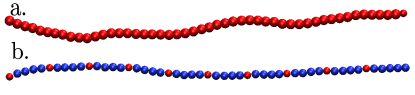
Figure 1: Figure displays arrangement of the active monomers on the filament in red color and passive monomers are in blue color. Top filament (a) corresponds for the homogeneous self-propulsion and the bottom one (b) is for the periodic sequence of the active monomers. Distance between two successive monomers is $l_{a}=5$ (in simulation units).

II Simulation Model

We model filament as a semiflexible linear polymer composed of a sequence of $N$ monomeric units connected via Harmonic spring. All the monomers in the polymer also interact via excluded volume interactions. The total potential energy of the filament can be written as, $U=U_{h}+U_{b}+U_{LJ}$, where $U_{h}$ is spring potential, $U_{b}$ is bending potential and $U_{LJ}$ corresponds to excluded volume potential. Harmonic potential is given as,

$$U_{h}=\frac{k_{s}}{2}\sum_{i=1}^{N-1}(|{\bm{r}}_{i+1}-{\bm{r}}_{i}|-l_{0})^{2},$$ (1)

where $l_{0}$ is average equilibrium bond length, ${\bf r}_{i}$ is position vector of the $i^{th}$ monomer, and $k_{s}$ is the spring constant. Bending potential energy $U_{b}$, which accounts for the stiffness of the polymer is written as,

$$U_{b}=\frac{\kappa}{2}\sum_{i=1}^{N-2}({\bm{R}}_{i+1}-{\bm{R}}_{i})^{2},$$ (2)

here $R_{i}$ is length of the $i^{th}$ bond vector, defined as ${\bf R}_{i}={\bf r}_{i+1}-{\bf r}_{i}$, and $\kappa$ is the bending rigidity of the polymer which can be expressed in terms of persistence length of the polymer $l_{p}$ as, $l_{p}=\kappa l_{0}^{3}/{k_{B}T}$, where $k_{B}T$ is thermal energy.

Excluded volume potential avoids overlap of beads in a polymer, and its form is taken from truncated repulsive part of Lennard-Jones potential, i.e., $R_{ij}<2^{1/6}\sigma$,

$$U_{LJ}=\sum_{i=1}^{N-1}\sum_{j=i+1}^{N}4\epsilon\left[\left(\frac{\sigma}{R_{ij}}\right)^{12}-\left(\frac{\sigma}{R_{ij}}\right)^{6}+\frac{1}{4}\right],$$ (3)

and for $R_{ij}\geq 2^{1/6}\sigma$, it is considered as, $U_{LJ}=0$. Here, $\epsilon$ is LJ interaction energy and $\sigma$ is LJ diameter of the monomer.

Newton’s equation of motion for a monomer in overdamped limit is,

$$\gamma\frac{d{\bm{r}_{i}}}{dt}=-\nabla_{i}U+\textbf{F}_{r}^{i}+\textbf{F}_{a}^{i},$$ (4)

where $\gamma$ is the friction coefficient, $\textbf{F}_{r}^{i}$ is the thermal noise with zero mean, and $\textbf{F}_{a}^{i}$ is the self-propulsion force which is exerted on the $i^{th}$ bond vector. Since hydrodynamics interactions are ignored in the simulations thereby solvent-mediated indirect coupling among the monomers is absent in the equation of motion.

The viscous drag and the thermal noise are related through the fluctuation-dissipation relation,

$$\left<\textbf{F}_{r}^{i}(t).\textbf{F}_{r}^{j}(t^{\prime})\right> = 6k_{B}T\gamma\delta_{ij}\delta(t-t^{\prime}).$$ (5)

Total self-propulsion force on the polymer is given as,

$$\textbf{F}_{a}^{T}=\sum_{i=1}^{N}{\bf F}_{a}^{i}=\sum_{i=1}^{N-1}f_{a}{\bf t}({\bf r}_{i})\Theta(r_{i}).$$ (6)

Where ${\bf t}({\bf r}_{i})={({\bm{r}}_{i+1}-{\bm{r}}_{i})}/{|{\bm{r}}_{i+1}-{\bm{r}}_{i}|}$ is unit tangent vector on the $i^{th}$ monomer. Active force is shared equally between $i^{th}$ and $(i+1)^{th}$ monomers as $f_{a}/2$. If step function $\Theta(r_{i})=1$, then $i^{th}$ monomer is active. Similarly if $\Theta(r_{i})=0$, then monomer will be passive. We consider here two different arrangements of self-propulsion force on the filament described as follows. i) Homogenous self-propulsion: Active force is applied on each bond of the polymer, therefore all monomers feel active force. We term it as homogenous self-propulsion. ii) Periodic sequence of self-propulsion: In this case, propulsion force is applied to few bonds arranged in a periodic sequence. Placement of active monomers starts from the tail of filament in equidistant manner with leaving front end as passive. Fig. 1b displays the clear picture of the periodic arrangement of active monomers on the filament.

In the periodic self-propulsion, number of active monomers are taken as a variable parameter which varies from $N_{a}=0$ to $N_{a}=N$. Here $N_{a}=0$ corresponds to the passive filament, while $N_{a}=N$ recovers the homogeneous self-propulsion. Strength of the active force is defined in units of thermal energy called as Péclet number, which is a dimensionless number. It is defined here as, $Pe=\frac{f_{a}l_{0}}{k_{B}T}$. In the limit of $Pe<<1$, thermal fluctuation dominates. However, in the limit of $Pe>>1$, active force dominates. The ratio of the Péclet number ($Pe$) and the scaled persistence length ($l_{p}/l_{0}$) is a dimensionless parameter given as, $\chi=l_{0}Pe/l_{p}$. Here, $\chi$ is called flexure number, which provides a measure of active force over the bending rigidity. Flexure number is used to understand the buckling instabilitiesSekimoto et al. (1995); Chelakkot et al. (2014), spontaneous spiral formation, spiral stability and rotational motionIsele-Holder et al. (2015, 2016) of active filaments.

All the physical parameters presented here are scaled in units of the bond length $l_{0}$, diffusion coefficient of a monomer $D_{m}$, and thermal energy $k_{B}T$. Simulations parameters are chosen as, $k_{s}=1000k_{B}T/l_{0}^{2}$, $\sigma=l_{0}$, $\epsilon/k_{B}T=1$, and time is in units of $\tau=l_{0}^{2}/D_{m}$, and stiffness parameter $\kappa$ is in units of $k_{B}T/l_{0}^{2}$. Separation between active sites are considered in the range of $l_{a}=1$ ($N_{a}=101$) to $l_{a}=25$ ($N_{a}=4$) and the bending rigidity of the polymer is varied in the range of $\kappa=0$ to $200$ for homogeneous self-propulsion, whereas for patterned case we take $\kappa=100$ and $\kappa=40$. Unless explicitly mentioned, number of monomers in the chain is taken to be $N=101$. We use Euler integration technique to solve Eq. 4. The integration time step $\Delta t$ is varied from the range of $10^{-2}\tau$ to $10^{-5}\tau$ to ensure stable simulation results. All the simulations are performed in cubic periodic box in three spatial dimensions.

All simulations are restricted in the range of Péclet number $0$ to $600$. A larger active force causes increase in the average bond length thus it requires larger spring constant. In addition to that, smaller integration time step needs to be taken into account for better numerical accuracy. In order to ensure better statistics, each data point is averaged over $50$ independent runs in small Péclet number limit,i.e., $Pe<1$. However, rest of the data points are averaged over 32 independent runs.

III Homogeneous Self-Propulsion

In this section, we present results for homogeneous self-propulsion where all monomers are active. In equilibrium, structural and dynamical behavior of the filament is very well understood in the pastWinkler et al. (1994); Harnau et al. (1997); Kratky and Porod (1949); Saitô et al. (1967); Hsu et al. (2010, 2011). The presence of propulsion on the filament causes bending, therefore its structural and dynamical behavior deviates from the equilibrium.

III.1 Structural Properties

The structural change is analysed by estimating average radius of gyration $R_{g}$, and average end-to-end distance $R_{e}$ of the filament. The radius of gyration and the end-to-end distance is computed by the expression,

$$R_{g}^{2}=\frac{1}{N}\left<\sum_{i=1}^{N}({\bm{r}}_{i}-{\bm{r}}_{cm})^{2}\right>~{};~{}R_{e}^{2}=\left<({\bm{r}_{1}}-{\bm{r}_{N}})^{2}\right>,$$ (7)

where ${\bm{r}}_{cm}$ is the centre-of-mass of the filament and angular brackets indicate the ensemble average of the physical quantities. Figure 2 shows the dependence of radius of gyration and end-to-end distance on flexure number for various bending rigidities.

First, we discuss results of the flexible polymer, i.e., for $\kappa=0$. In the weak active force,i.e., $\chi<<1$, the normalised radius of gyration $R_{g}/R_{g}^{0}$ decreases monotonically with increasing $\chi$. Further increase in $\chi$ results relatively large change in $R_{g}/R_{g}^{0}$ and eventually in the limit of large $\chi>10$, $R_{g}$ is almost independent of $\chi$, which is consistent with other simulations and theoretical resultsEisenstecken et al. (2017, 2016). The saturation in $R_{g}$ and $R_{e}$ occurs due to excluded volume interactions which prevents collapse of a polymer.

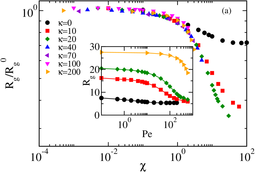
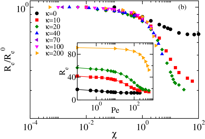
Figure 2: Figure shows the relative change in the mean radius of gyration $R_{g}/R_{g}^{0}$ (Plot a) and the end-to-end distance $R_{e}/R_{e}^{0}$ (Plot b) w.r.t. its equilibrium values $R_{g}^{0}$ and $R_{e}^{0}$ respectively as a function of flexure number $\chi$. Inset of figure a and b shows the mean radius of gyration and the mean end-to-end distance $R_{e}$ as a function of $Pe$. Various curves in figure a and b corresponds to $\kappa$ as displayed in the figures.

Now we present results for the semiflexible filament. Here, the radius of gyration decreases with activity as displayed in figure 2. In the limit of weak active force, i.e., $\chi<1$, the radius of gyration gradually decreases with $\chi$ similar to the flexible polymer. Further increase in active force, i.e., $\chi\geq 1$, the relative change in the radius of gyration increases substantially. Interestingly, for $\kappa>10$, all the curves display nearly a universal behavior up to four orders of magnitude in $\chi$ as shown in figure 2. The end-to-end distance also reflects the same universal trend whose properties can be understood in terms of a single master curve in limit of $\chi<10$. In the semiflexible regime, $R_{g}$ and $R_{e}$ decreases monotonically with $\chi$ up to $\chi\sim 1$. For $\chi>>1$, $R_{g}$ approaches to a plateau value for $\kappa=10$ and $20$ similar to the flexible polymer limit as reflected in Fig. 2a and 2b. The inset of Fig. 2 a and b display absolute values of $R_{g}$ and $R_{e}$ as a function of $Pe$ for various $\kappa$. This reflects the monotonic decrease of $R_{g}$ and $R_{e}$ in the range of $Pe\leq 10^{2}$. For the $\kappa\leq 20$, $R_{g}$ and $R_{e}$ are slowly approaching to a saturation limit. Note that for $\kappa>20$, the saturation limit is not reached in displayed simulation range, which will appear in the limit of $Pe>10^{3}$.

A filament shrinks under homogenous self-propulsion due to several competitive forces on it, which can be understood in terms of fluctuations in bond orientations due to random motion of monomers. As a bead always goes to random motion which causes fluctuations in bond orientations along the contour. Hence tangential force pushes filament along the randomly fluctuating bond directions, which leads to increase in the average noise over the filament. Thus it bends and buckles with $Pe$, which results in the shrinkage of the filament. Considerably larger values of $\kappa$ suppress bond fluctuations, thus shrinkage of the polymer is smaller, even for the substantially large Péclet numbers.

The shrinkage in the radius of gyration with activity reflects a decrease in the rigidity of the polymer. To quantify the change in the rigidity, we compute its persistence length with active force. This can be computed from the tangent-tangent auto-correlation of the filament, which is expressed as, $C(s)=<{\bf t}({\bm{r}_{i}})\cdot{\bf t}({\bm{r}_{1})}>$, where $s$ is the arc length, $s=|r_{i}-r_{1}|\equiv|i-1|$. We have estimated correlation from one end of the polymer, i.e., from the tail for $i=1,2...N-1$. The correlation decays exponentially as, $C(s)\sim\exp(-\frac{s}{l_{p}})$, with the arc length of the polymer for all values of $Pe$ and $\kappa$. We calculate persistence length by fitting exponential function in the correlation function. Figure 3 displays the persistence length as a function of $\chi$, as expected, $l_{p}$ decreases monotonically for all $\kappa$ in the limit of $\chi\leq 1$. In the limit of $\chi>1$, active polymer becomes flexible thereby persistence length, $l_{p}\approx l_{0}$, thus in the activity dominated regime $\chi>1$, $l_{p}$ nearly saturates as displayed in figure 3 for smaller $\kappa=10$ and $20$. In the limit of $\chi\leq 1$, all the curves display a universal behavior with $\kappa$ as illustrated in the plot. The analysis of the persistence length suggests that a semiflexible polymer behave as a flexible polymer in the limit of large $\chi>10$.

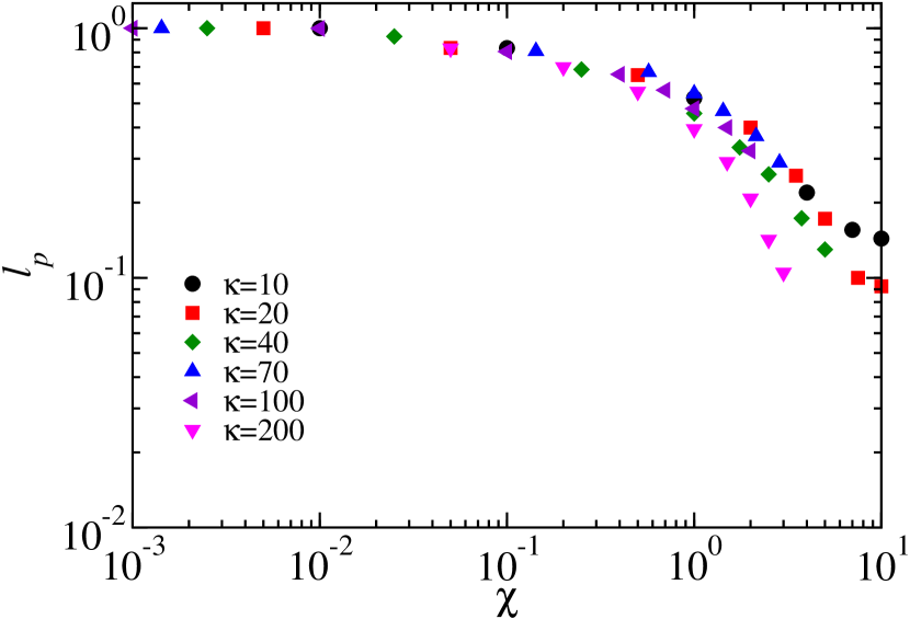
Figure 3: The persistence length $l_{p}$ as a function of $\chi$ for various $\kappa=10,20,40,70,100$ and $200$ for the polymer length $N=101$.

III.2 Diffusion of Filament

In this section, we discuss dynamics of a filament under homogeneous self-propulsion by estimating mean-square-displacement(MSD) of the centre-of-mass. The MSD of a filament is computed as, $<R_{cm}^{2}(t)>=<[r_{cm}(t)-r_{cm}(0)]^{2}>$, where angular bracket denotes ensemble average. In equilibrium, qualitative behavior of the MSD of a filament can be separated in mainly two time regimes. The short-time limit is called ballistic regime, where $<R_{cm}^{2}(t)>\sim t^{2}$, however long-time limit is called diffusive regime, here the MSD varies linearly in time given as, $<R_{cm}^{2}(t)>=6Dt$, where $D$ is the diffusion coefficient of the filament. Fig.4, displays the MSD of the filament with time for different $Pe$. The MSD of the passive filament is shown from the solid line. As expected, it reflects diffusive behavior in the long-time limit.

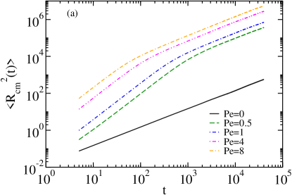
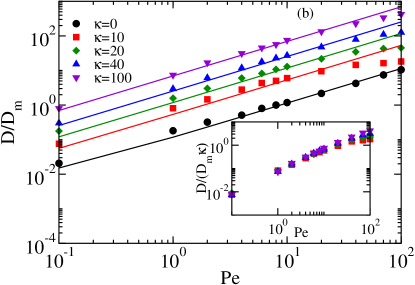
Figure 4: a) The mean-square displacement of the centre-of-mass of the filament for $\kappa=40$ for various $Pe=0.0,0.5,1,4$ and $8$. b) The scaled effective diffusivity $D/D_{m}$ of the filament as a function $Pe$ for various $\kappa=0,10,20,40$ and $100$. Inset shows scaled diffusivity $D/(D_{m}\kappa)$ with $Pe$ for $\kappa=10,20,40$ and $100$.

In the presence of tangential active force, the polymer is compressed and drifted along the end-to-end vector. Drift motion reflects the enhanced mean-square-displacement of the centre-of-mass in the intermediate time regime. Increase in the MSD is observed with $Pe$ in all time regimes. It is evident from the plot, the MSD exhibits superdiffusive behavior,i.e., $<R_{cm}^{2}>\sim t^{\alpha}$, with exponent $\alpha>1$, in the intermediate time regime. In the long time limit, the MSD recovers the linear behavior. Another interesting observation is the shift in timescale of super-diffusive regime to smaller time with Péclet number. This can be interpreted in terms of the flexibility and memory of directed motion. A filament becomes flexible with active force as shown in the structural analysis, which results decrease in the persistence length of the directed motion. Thereby, superdiffusive behavior persists relatively at smaller time. In a more intuitive way, we can also derive an approximate expression for the crossover time by equating the MSD expression in ballistic regime $<R_{cm}^{2}(t_{c})>\sim(f_{a}t_{c}/\gamma)^{2}$, and diffusive regime $<R_{cm}^{2}(t_{c})>\sim Dt_{c}$, which gives $t_{c}\sim D\gamma^{2}/f_{a}^{2}$.

The long time diffusivity of the filament is obtained by fitting a linear function to the MSD curves. Figure 4b displays diffusivity of the polymer with $Pe$ for several values of the rigidities. The diffusivity enhances with the Péclet number. Moreover, it increases linearly with $Pe$, as, $D\sim g(\kappa)Pe$, where $g(\kappa)$ shows bending dependence of $D$, for all $\kappa$ as illustrated in Fig. 4. The effective diffusivity of the filament increases due to active fluctuations in the system. In an active medium, a modified form of the fluctuation-dissipation-relation(FDR) is proposed that relates the measured effective diffusivity of a tracer particle with effective temperature as, $D=k_{B}T_{eff}/\gamma$ Loi et al. (2011); Palacci et al. (2010). We use above relation to define the effective temperature $T_{eff}$ in terms of long time diffusivity of the filament. Thus the effective temperature of the filament increases with active force as also reported in Ref. Ghosh and Gov (2014).

The crossover time $t_{c}$ defined above can be re-expressed in terms of $Pe$ and effective diffusivity as $t_{c}\sim D/Pe^{2}$, linear dependence of $D$ on $Pe$ gives $t_{c}\sim g(\kappa)/Pe$. Inset of Fig. 4b shows that $D/(\kappa D_{m})\sim Pe$,i.e., $g(\kappa)\sim\kappa$. Hence, we obtain, $t_{c}\sim\chi^{-1}$. Thus the crossover time decreases with increasing $\chi$, our simulation also shows decreases in $t_{c}$ with $\chi^{-1}$.

The linear form of the diffusivity of a filament with $Pe$ near the surfaces is also reported in previous studiesIsele-Holder et al. (2015, 2016). At large bending parameters, persistence length of the directional motion increases therefore the diffusivity also increases, which shows linear increase as expected with $\kappa$ for a given Péclet number. Thus, a stiffer filament diffuses relatively faster than the flexible polymer under homogeneous self-propulsion.

IV Periodic Sequence of Active Force

In this section, we explore various conformations of the filament under equally spaced active monomers. Leaving front monomers as passive, which acts as a load, leads to bending of the filament under compression. Presence of activity on the front monomers pull the front beads, which suppress the buckling between front active monomers. In addition to this, it also drags the filament along the same direction that leads to translation motion. Thereby, front monomers are always left as passive. Importance of load is discussed and analysed in the conclusion section for the case of inhomogeneous self-propulsion.

The arrangement of the active force on the filament is shown in Fig. 1 for the separation $l_{a}=5$. Here, $l_{a}$ is the distance between two successive active monomers. Interestingly, under a periodic sequence of active force, a filament acquires interesting conformations during motion which is not observed in homogenous self-propulsion in bulk. These conformations depend on the spacing between active forces $l_{a}$, the strength of propulsion and the rigidity of the filament.

In small Péclet number $Pe<1$, filament translates along the direction of end-to-end vector, thus its structure is weakly perturbed. In the intermediate regime of compressive force, external force becomes comparable to the elastic energy. Therefore an active monomer pushes against passive monomers, which causes bending of the filament. Further increase in the force buckles the filament in a correlated manner throughout the filament. This occurs for the separation of the active monomers $l_{a}\geq 5$. In case of correlated buckling, it forms a circular or helical structure. Circular phase appears in the range of $l_{a}\geq 14$ and narrow range of $Pe$. In our analysis, a circular phase is treated as helical phase. This can be visualised as a circular structure is a helix of one helical turn with very small pitch length. Further increase in the force pushes filament strongly against the viscous drag, which causes uncorrelated buckling and it leads to distortion in the structure. Large force results to sharp bending and twisting of the filament nearby the active monomers, such sharply bent structures are called folded structures here.

Few snapshots of the filament in the extended, helical, circular and folded states are shown in figure 5. We have also shown these structures in supplementary movie files in $S1$, $S2$ and $S3$. Our focus in this section is to identify helical, circular and folded states of a self-propelled filament in the parameter space of $Pe$ and $l_{a}$. To do so, we compute two-point tangent-tangent correlation of the bond vectors, the bending energy and the torsional order parameter of the filament.

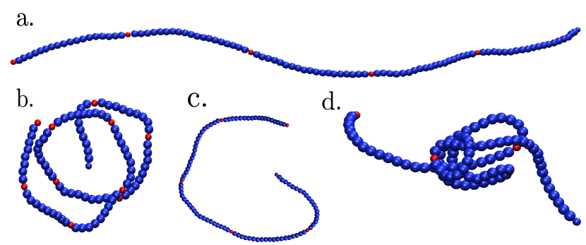
Figure 5: Few snapshots of the filament showing different structures under periodic arrangement of active monomers. Red color corresponds for the active monomer and blue color represents for the passive one. Top row represents for the extended state (a). In the bottom row helical(b), circular(c) and folded structures(d) are shown form left to right respectively.

IV.1 Helical Phase

A helical phase can be distinguished using tangent-tangent correlation of the filament. The characteristic behavior of helical state is function of $l_{a}$ and $Pe$. To quantify the helical state in above parameter space, we compute tangent-tangent correlation function of the filament as discussed earlier. Fig. 6 shows variation of the correlation for few Péclet numbers at $l_{a}=10$. Here the correlation is computed from the end monomers as a function of arc length $s$. The correlation function $C(s)$ decays exponentially in the weak force limit with $s$. For larger force,i.e.,$Pe=20$, correlation sharply reaches to negative values after approaching to a minimum it tends to zero from the negative side. Further increase in the $Pe$ shows oscillations in the correlation. At larger $Pe$, these oscillations show long-range correlation. Strong correlation and sinusoidal behavior signify the underlying helical phase of the filamentGiomi and Mahadevan (2010). Note that, under homogenous self-propulsion oscillatory behavior in the correlation is absent throughout the parameter regime presented in this article. Hence, we conclude that no helical structure occurs in this case. Therefore, crossover from the exponential to sinusoidal correlation is the signature of a helical phase. Sinusoidal behavior of correlation occurs in both circular and helical phases.

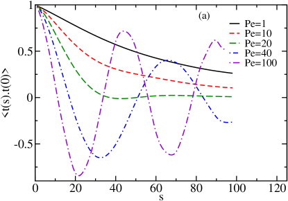
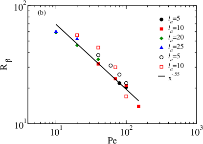
Figure 6: a) Figure displays tangent-tangent correlation function $<{\bf t}(s)\cdot{\bf t}(0)>$ of the self-propelled filament at $l_{a}=10$ and bending rigidity $\kappa=100$. b) Figure displays curvature radius $R_{\beta}$ of the helical phase obtained from fitting Eq. 8 for various $l_{a}=5,10,20$ and $25$ for $\kappa=100$ (filled symbols). Open symbols corresponds for $l_{a}=5$ and $10$ at $\kappa=40$. The solid line shows power behavior $\left({Pe}\right)^{-.55}$ of the curvature radius.

A characteristic length scale and wave number associated with the correlation can be estimated from the following expression,

$$C(s)=a_{\beta}\exp(-s/l_{p})(\cos(2\pi s/R_{\beta}),$$ (8)

where $a_{\beta}$ is some constant and $R_{\beta}$ is the length scale associated with the curvature radius of the filament. This function exhibits the property that it decays exponentially and captures oscillatory behavior also. Fitting Eq. 8 in the tangent-tangent correlation gives the curvature of the filament, which is plotted in Fig. 6 as a function of $Pe$. As expected, curvature radius decreases with increasing compressive force. Interestingly, $R_{\beta}$ for all the $l_{a}$’s shows a similar trend and it follows a master curve without any scaling parameter as shown in the graph. Moreover, the master curve exhibits a power law behavior with Péclet number, as $R_{\beta}\sim Pe^{-\beta}$, with the exponent $\beta\sim 0.55$. The solid line in Fig. 6 is shown for visualisation of the power law behavior with the same exponent. The curvature radius of the filament obtained here has slightly larger exponent compare to a buckled filament near the surfacesChelakkot et al. (2012), which we believe due to larger contour fluctuations in the bulk relative to the surfaces.

To show out of plane motion and twist of the filament in the helical phase, we compute average torsional order parameter of the filament. This is computed in a manner similat to that discussed in Ref. Chelakkot et al. (2012),

$$U_{t} = \sum_{i=2}^{N-1}\frac{1}{N-3}\cos{\theta_{i}},$$ (9)

$$\cos{\theta_{i}} = \frac{(\vec{R}_{i-1}\times\vec{R}_{i}).(\vec{R}_{i}\times\vec{R}_{i+1})}{|\vec{R}_{i-1}\times\vec{R}_{i}||\vec{R}_{i}\times\vec{R}_{i+1}|},$$

here $U_{t}$ is average of the sum of cosines of the torsion angle over the filament and $\theta_{i}$ is the angle given by three consecutive bond vectors $\vec{R}_{i-1},\vec{R}_{i}$ and $\vec{R}_{i+1}$. Figure 7 displays $U_{t}$ with Péclet number for various $l_{a}$. The torsional order parameter smoothly increases with $Pe$. Figure 7 displays $U_{t}$ that is very small in the limit of $Pe<<1$, further increase in $Pe$ leads to a monotonic increase in the torsional order parameter. In the limit of large $Pe$, $U_{t}$ has increased nearly two orders of magnitude. Large values of $U_{t}$ signifies that filament can be strongly twisted or folded, but it’s not sufficient enough to delineate the helical structure. The combination of torsional order parameter and tangent-tangent correlation can precisely define the helical state. It would be important to mention here that torsional angle does not reflect any sharp transition from extended to helical and later state to folded state. Rather it varies smoothly from one phase to another phase with forceKemp and Chen (1998).

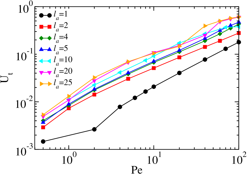
Figure 7: Average torsional order parameter $U_{t}$ as a function of $Pe$ for various $l_{a}$ as shown in the figure for a given $\kappa=100$.

Another interesting observation worth mentioning here is the increase in the torsional parameter with $l_{a}$ for a given $Pe$. Fewer active monomers produce large amount of twist or out of plane motion to the filament. In the limit of small separations, translation motion is dominant thus the change in torsional parameter is small. Increasing separations cause a larger drag force on the active monomers and thus reduce the translation motion, which buckles the filament between active locations. This is reflected in the increase in torsion order parameter, from this we infer that in order to have a correlated buckling large separation among the active monomers is essential.

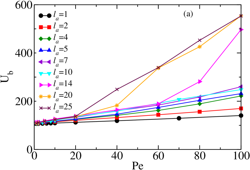
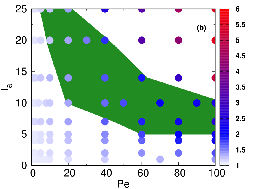
Figure 8: a) Average bending energy of the filament as a function of $Pe$ for various spacing between active monomers. b) Phase diagram for the equispaced activity on the polymer for a given $\kappa=100$. The light blue circle on the graph shows extended structure, green shaded area represents the helical and circular structures. Above the green shaded area the folded state is represented. In order to accomodate equal spacing between the active monomers we have taken filament length $N=99$ for the $l_{a}=7$ and $14$.

IV.2 Folded state

In this section, we quantify uncorrelated buckling of the filament. In the limit of large force, helical or circular states are followed by folded state. In this structure, a filament is strongly folded near the active monomers due to large buckling. To distinguish the helical state from the folded state, we compute the bending energy of the filament. Figure 8a displays variation of bending energy of the filament with $Pe$. Bending energy increases linearly with $Pe$ in the range of $l_{a}<14$. For the $l_{a}>14$, bending energy increases monotonically up to a certain Péclet number, after which an abrupt change in the bending energy appears specifically for $l_{a}=14,20$ and $25$ as shown the Fig .8a. The transition point from the helical to the folded state is recognised from the sharp increase in the bending energy.

A sudden increase in the bending energy arises from the sharp buckling of the filament, which is uncorrelated over the length scale of $l_{a}$. Therefore, sharp buckled filament exhibits very high bending energy. Once again it’s important to mention here that elastic or bending energy does not show any sharp transition between the extended state to the helical or circular state. However, a folded state does show sharp increase in the elastic energy. Furthermore, bending energies of the circular and the helical states exhibit similar behavior.

From the analysis of torsional order parameter, the bending energy, and the tangent-tangent correlation different structures of the filament in the parameter space of $Pe$ and spacing between active forces are recognised. A phase diagram is displayed in the Fig. 8b as a function of $Pe$ and $l_{a}$. A color map shows the variation in bending energy per monomer in different phases, similarly color of the symbols are also changed in the plot. In graph, extended state and uncorrelated folded state are separated by the green shaded area which reflects the helical and circular states.

In the green shaded area, a circular phase appears for $l_{a}=14,20$ and $25$ and a helical is for $l_{a}=5,7$ and $10$. We are analysing various structures in terms of bond correlation, torsional energy, and bending energy. These physical quantities do not show any significant change from a circular to helical states as displayed in figures 6, 7, and 8a. Thus in the phase diagram, a circular state is displayed together with the helical state. The region below the green shaded area represents the extended state, and above the shaded area corresponds to the folded state. Below the green area an extended phase appears, which occurs in smaller separation limit $l_{a}\leq 4$ for all $Pe$. In addition to that, for large separations extended state appears in the limit of small Péclet number.

V Summary and conclusions

In this article, we have performed a detailed study of the structural and dynamical behavior of a freely moving self-propelled filament in three dimensions. The location and the number of self-propelled monomers are considered as a variable, and they are mimicked in two different ways, homogeneously, i.e., on all monomers and periodic sequence of the self-propulsion on the filament.

In the homogeneous self-propulsion, the radius of gyration and the end-to-end distance decreases with increasing active force for all the bending parameters. We have shown that the change in structural properties for various rigidities can be described by flexure number with a single master curve in the limit of $\chi\leq 1$. Similarly, our analysis also reveals that the persistence length of the polymer decreases with active force, a universal behavior for all bending parameters is also shown in the limit of $\chi\leq 1$. The translation motion is dominant for $\chi<<1$, thus it acquires the extended state. In the limit of $\chi\approx 1$ the polymer gradually enters from semiflexible to flexible limit where it acquires coil-like structure. The later state is more favourable in the presence of large fluctuations due to higher entropy.

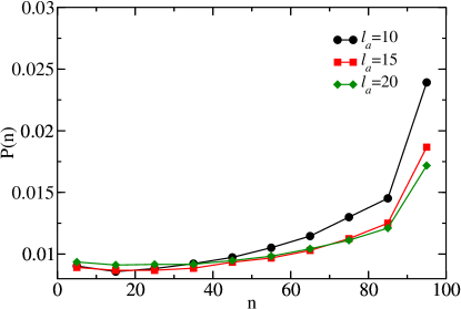
Figure 9: The distribution of active sites on the filament for the rod-like structure. Here $n=100$ corresponds to the head (front monomer) of the filament and $n=1$ is the tail.

The sequential arrangement of active monomers shows the large-scale conformational transition even at fewer number of active monomers and small force limit. In this case, filament acquires extended, circular, helical, and folded structures. A helical or circular phase appears for larger separation of active monomers $l_{a}\geq 5$ and under strong compressive force $Pe>1$. For the larger separations smaller activity is sufficient for the formation of helical structure. This state occurs due to the competition among drag, active and bending forces. A larger load applies more drag on the active monomers that requires larger force to push the filament. If active force is weaker to drag the passive monomers then active energy is converted into buckling of the filament. The transition point is recognised from the tangent-tangent correlation, which shows crossover from exponential decay to oscillatory behavior Giomi and Mahadevan (2010). Large torsional order parameter also confirms twisting and long-range ordering of bonds on the filamentChelakkot et al. (2012).

The load in a patterned case is very crucial at intermediate separations. Several interesting structures appear for large separations,i.e., $l_{a}\geq 5$. Here, polymer buckles under the load in front of active monomer that translates to all over polymer due to large separation among the active monomers. This leads to the rotation of the filament. Thus the presence of load and regular arrangement of the activity causes correlated buckling which eventually translated in circular, helical or folded structures with $Pe$. On the other hand, if the first monomer is also considered as an active for $l_{a}\geq 5$ (without load) then it pulls the filament from the front end, which suppresses buckling between first two active monomers and causes translation of the filament.

Furthermore, to display importance of the load on the active filaments, we perform simulations with randomly placed active monomers termed here inhomogeneous self-propulsion. In this case, few monomers are randomly chosen to be active whose locations are also shuffled at new uncorrelated locations with time. The shuffling is done in the fixed time interval chosen in such a way that it is larger than the longest relaxation time of the filament. A filament acquires structures similar to the periodic arrangement, these structures display a strong correlation with the location of the active monomers and their numbers.

We choose to analyse here only rod-like state under inhomogeneous self-propulsion. If $R_{e}\geq 0.9Nl_{0}$, then it is assumed to be in the rod-like state. We compute the distribution of active monomers over the filament for $R_{e}\geq 0.9Nl_{0}$. In other words, we identify the probability distribution of active monomers for a rod-like structure under inhomogeneous self-propulsion. The distribution of active sites (Fig. 9) reflects the probability of front few monomers to be active is nearly $3$ times higher relative to others. This can be interpreted as presence of large number of active sites in the front drags the filament easily through medium therefore it may always stay in the extended state. The structure is similar to pulling a filament by a constant force. Therefore, the presence of a load is very crucial for the transition from the extended to helical, circular and folded states.

A filament under inhomogeneous viscous drag often buckles in a helical or U-shape structures Chelakkot et al. (2012); Steinhauser et al. (2012). Such structures are very common in the biological systems, for example beating motion of the sperms,C.elegans, and helical structure of flagellum in the bacteriaElgeti et al. (2015); Marchetti et al. (2013); Bechinger et al. (2016). In summary, we have identified that a freely swimming filament acquires helical phase in the presence of load at the front end which is so far have not been investigated in previous study. The curvature radius of the filament shows a power law behavior as, $R_{\beta}\sim Pe^{-\beta}$ , $\beta\sim 0.55$. The strong buckling of the filament under the periodic arrangement of active force may provide insight in the understanding of mechanical response of the actin filaments in the presence of molecular motors Sanchez et al. (2012, 2011). It would be interesting to explore the conformations of the filament under the inhomogeneous self-propulsion in detail. This case may be able to provide a better comparison from the experimental systems where the medium is more complex and heterogeneous.

VI Acknowledgment

We thank funding agency DST SERB project grant no. YSS/02015/000230 for the financial support. Authors acknowledge the high performance computing facility at IISER Bhopal for the computation time.

References

- Vicsek et al. (1995) T. Vicsek, A. Czirók, E. Ben-Jacob, I. Cohen, and O. Shochet, Physical review letters 75, 1226 (1995).
- Parrish and Hamner (1997) J. K. Parrish and W. M. Hamner, Animal groups in three dimensions: how species aggregate (Cambridge University Press, 1997).
- Dombrowski et al. (2004) C. Dombrowski, L. Cisneros, S. Chatkaew, R. E. Goldstein, and J. O. Kessler, Physical review letters 93, 098103 (2004).
- Marchetti et al. (2013) M. C. Marchetti, J. F. Joanny, S. Ramaswamy, T. B. Liverpool, J. Prost, M. Rao, and R. A. Simha, Rev. Mod. Phys. 85, 1143 (2013).
- Elgeti et al. (2015) J. Elgeti, R. G. Winkler, and G. Gompper, Reports on Progress in Physics 78, 056601 (2015).
- Bechinger et al. (2016) C. Bechinger, R. Di Leonardo, H. Löwen, C. Reichhardt, G. Volpe, and G. Volpe, Rev. Mod. Phys. 88, 045006 (2016).
- Ghosh and Gov (2014) A. Ghosh and N. Gov, Biophysical Journal 107, 1065 (2014), ISSN 0006-3495.
- Eisenstecken et al. (2016) T. Eisenstecken, G. Gompper, and R. G. Winkler, Polymers 8, 304 (2016).
- Eisenstecken et al. (2017) T. Eisenstecken, G. Gompper, and R. G. Winkler, The Journal of Chemical Physics 146, 154903 (2017).
- Jiang and Hou (2014) H. Jiang and Z. Hou, Soft Matter 10, 1012 (2014).
- Kaiser et al. (2015) A. Kaiser, S. Babel, B. ten Hagen, C. von Ferber, and H. Löwen, The Journal of Chemical Physics 142, 124905 (2015), eprint http://dx.doi.org/10.1063/1.4916134.
- Chelakkot et al. (2012) R. Chelakkot, R. G. Winkler, and G. Gompper, Phys. Rev. Lett. 109, 178101 (2012).
- Isele-Holder et al. (2015) R. E. Isele-Holder, J. Elgeti, and G. Gompper, Soft Matter 11, 7181 (2015).
- Isele-Holder et al. (2016) R. E. Isele-Holder, J. Jager, G. Saggiorato, J. Elgeti, and G. Gompper, Soft Matter 12, 8495 (2016).
- Laskar and Adhikari (2017) A. Laskar and R. Adhikari, New Journal of Physics 19, 033021 (2017).
- Sarkar and Thakur (2016) D. Sarkar and S. Thakur, Physical Review E 93, 032508 (2016).
- Howard et al. (2001) J. Howard et al., Mechanics of motor proteins and the cytoskeleton (Sinauer associates Sunderland, MA, 2001).
- Brennen and Winet (1977) C. Brennen and H. Winet, Annual Review of Fluid Mechanics 9, 339 (1977).
- Lyons et al. (2006) R. Lyons, E. Saridogan, and O. Djahanbakhch, Human reproduction update 12, 363 (2006).
- Rodriguez et al. (2003) O. C. Rodriguez, A. W. Schaefer, C. A. Mandato, P. Forscher, W. M. Bement, and C. M. Waterman-Storer, Nature cell biology 5, 599 (2003).
- Vicsek and Zafeiris (2012) T. Vicsek and A. Zafeiris, Physics Reports 517, 71 (2012).
- Abkenar et al. (2013) M. Abkenar, K. Marx, T. Auth, and G. Gompper, Physical Review E 88, 062314 (2013).
- DeCamp et al. (2015) S. J. DeCamp, G. S. Redner, A. Baskaran, M. F. Hagan, and Z. Dogic, Nature materials 14, 1110 (2015).
- Sumino et al. (2012) Y. Sumino, K. H. Nagai, Y. Shitaka, D. Tanaka, K. Yoshikawa, H. Chaté, and K. Oiwa, Nature 483, 448 (2012).
- Schaller et al. (2011) V. Schaller, C. Weber, E. Frey, and A. R. Bausch, Soft Matter 7, 3213 (2011).
- Schaller and Bausch (2013) V. Schaller and A. R. Bausch, Proceedings of the National Academy of Sciences 110, 4488 (2013).
- Chelakkot et al. (2014) R. Chelakkot, A. Gopinath, L. Mahadevan, and M. F. Hagan, Journal of The Royal Society Interface 11, 20130884 (2014).
- Samanta and Chakrabarti (2016) N. Samanta and R. Chakrabarti, Journal of Physics A: Mathematical and Theoretical 49, 195601 (2016).
- Vandebroek and Vanderzande (2015) H. Vandebroek and C. Vanderzande, Phys. Rev. E 92, 060601 (2015).
- Osmanovic and Rabin (2017) D. Osmanovic and Y. Rabin, Soft Matter 13, 963 (2017).
- Maharana et al. (2012) S. Maharana, D. Sharma, X. Shi, and G. Shivashankar, Biophysical journal 103, 851 (2012).
- Talwar et al. (2013) S. Talwar, A. Kumar, M. Rao, G. I. Menon, and G. Shivashankar, Biophysical journal 104, 553 (2013).
- Weber et al. (2012) S. C. Weber, A. J. Spakowitz, and J. A. Theriot, Proceedings of the National Academy of Sciences 109, 7338 (2012).
- Zidovska et al. (2013) A. Zidovska, D. A. Weitz, and T. J. Mitchison, Proceedings of the National Academy of Sciences 110, 15555 (2013).
- Brangwynne et al. (2008) C. P. Brangwynne, G. H. Koenderink, F. C. MacKintosh, and D. A. Weitz, Physical review letters 100, 118104 (2008).
- Giomi and Mahadevan (2010) L. Giomi and L. Mahadevan, Physical review letters 104, 238104 (2010).
- Sekimoto et al. (1995) K. Sekimoto, N. Mori, K. Tawada, and Y. Y. Toyoshima, Phys. Rev. Lett. 75, 172 (1995).
- Winkler et al. (1994) R. G. Winkler, P. Reineker, and L. Harnau, The Journal of chemical physics 101, 8119 (1994).
- Harnau et al. (1997) L. Harnau, R. G. Winkler, and P. Reineker, The Journal of chemical physics 106, 2469 (1997).
- Kratky and Porod (1949) O. Kratky and G. Porod, Journal of Colloid Science 4, 35 (1949), ISSN 0095-8522.
- Saitô et al. (1967) N. Saitô, K. Takahashi, and Y. Yunoki, Journal of the Physical Society of Japan 22, 219 (1967).
- Hsu et al. (2010) H.-P. Hsu, W. Paul, and K. Binder, EPL (Europhysics Letters) 92, 28003 (2010).
- Hsu et al. (2011) H.-P. Hsu, W. Paul, and K. Binder, EPL (Europhysics Letters) 95, 68004 (2011).
- Loi et al. (2011) D. Loi, S. Mossa, and L. F. Cugliandolo, Soft Matter 7, 10193 (2011).
- Palacci et al. (2010) J. Palacci, C. Cottin-Bizonne, C. Ybert, and L. Bocquet, Physical Review Letters 105, 088304 (2010).
- Kemp and Chen (1998) J. P. Kemp and Z. Y. Chen, Phys. Rev. Lett. 81, 3880 (1998).
- Steinhauser et al. (2012) D. Steinhauser, S. Köster, and T. Pfohl, ACS Macro Letters 1, 541 (2012).
- Sanchez et al. (2012) T. Sanchez, D. T. Chen, S. J. DeCamp, M. Heymann, and Z. Dogic, Nature 491, 431 (2012).
- Sanchez et al. (2011) T. Sanchez, D. Welch, D. Nicastro, and Z. Dogic, Science 333, 456 (2011).