Dynamics of ferromagnetic domain walls under extreme fields

Abstract

We report the existence of a new regime for domain wall motion in uniaxial and near-uniaxial ferromagnetic nanowires, characterised by applied magnetic fields sufficiently strong that one of the domains becomes unstable. There appears a new stable solution of the Landau-Lifshitz-Gilbert equation, describing a nonplanar domain wall moving with constant velocity and precessing with constant frequency. Even in the presence of thermal noise, the new solution can propagate for distances on the order of 500 times the field-free domain wall width before fluctuations in the unstable domain become appreciable.

The dynamical response of magnetic domains in ferromagnetic nanostructures to applied fields and spin-polarized currents offers rich physics Tatara and Kohno (2004); Beach et al. (2005); Hayashi et al. (2007, 2008); Thomas et al. (2010), presents unresolved mathematical challenges Braun (2012); Hellman et al. (2017), and promises exciting technological applications Allwood et al. (2005); Parkin et al. (2008). Of particular importance is the problem of domain wall motion, in which a ferromagnetic material has two neighbouring magnetic domains, one expanding and the other contracting under the action of an applied field. To date, this problem has been addressed, analytically and numerically, in nanoscale systems with a variety of geometries and topologies, including tubes, ribbons and films (see e.g. Refs. Yan et al. (2011); Goussev et al. (2014); Depassier (2014); Gaididei et al. (2014, 2017); Boulle et al. (2013)). Here we focus on the important case of ferromagnetic nanowires Braun (2012); Tatara et al. (2008); Thiaville and Nakatani (2006); Goussev et al. (2013).

A common feature of most of these studies (but cf Refs. Depassier (2015); Benguria and Depassier (2016), discussed below) is the assumption that the applied field is not strong enough to destabilise either domain. Here, we consider the case of applied fields sufficiently strong that one of the two domains becomes intrinsically unstable. We show that there emerges a fast-travelling precessing domain wall with nonplanar profile – see Fig. 1, and calculate its velocity and precession frequency. We estimate the lifetime of the domain wall in the presence of thermal noise; for realistic parameters, it can travel 500 times the field-free domain-wall width before being overtaken by thermal fluctuations.

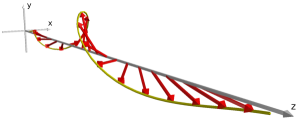
Figure 1: High-field domain wall with tail-to-tail boundary conditions. The envelope (yellow curve) of the magnetisation (red arrows) indicates a helical as opposed to planar profile. The asymptotic sense and pitch of the helix may be interpreted in terms of the chirality and wavelength of entrained spin waves.

We start from a standard model for domain wall dynamics under an applied field $H_{a}\bm{\hat{z}}$, taking the wire to be one dimensional along the $z$-axis. For definiteness, we take $H_{a}>0$. The evolution of the magnetisation, $M_{s}\bm{m}(z,t)$, where $M_{s}$ is the fixed saturation magnetisation and the unit-vector $\bm{m}=(m_{1},m_{2},m_{3})$ determines orientation, is governed by the Landau-Lifshitz-Gilbert (LLG) equation,

$$\partial_{t}\bm{m}=\gamma\bm{H}\times\bm{m}+\alpha\bm{m}\times\partial_{t}\bm{m}\,,$$ (1)

where $\bm{H}=-(M_{s})^{-1}\delta E/\delta\bm{m}+H_{a}\bm{\hat{z}}$ is the effective magnetic field, $\gamma$ the gyromagnetic ratio and $\alpha$ the Gilbert damping constant (typically $\alpha\ll 1$). The micromagnetic energy per unit cross-sectional area is given by

$$E=\tfrac{1}{2}\int\left(A\left|\partial_{z}\bm{m}\right|^{2}+K(1-m_{3}^{2})+K_{2}m_{2}^{2}\right)dz,$$ (2)

where $A$ is the exchange constant and $K,K_{2}\geq 0$ are the anisotropy constants along the (easy) $z$- and (hard) $y$-axes. The spatially uniform domains $\bm{m}=\pm\bm{\hat{z}}$ are global minimisers of the energy, so that boundary conditions appropriate for a (head-to-head) domain wall are $\bm{m}(\pm\infty,\cdot)=\mp\bm{\hat{z}}$. This description incorporates several simplifications, including reducing to one dimension and incorporating the magnetostatic energy into the local anisotropy; see Sanchez (2009); Slastikov and Sonnenberg (2012) for discussion and justification.

The model (1)–(2) has been extensively analysed in the literature (see e.g. Schryer and Walker (1974); Malozemoff and Slonczewski (1979); Kosevich et al. (1990); Thiaville and Nakatani (2006); Yan et al. (2010); Goussev et al. (2010, 2013); Slastikov et al. (2019)). We will restrict our attention to the case of near-uniaxial wires, for which $K\gg K_{2}$ (eventually, we will take $K_{2}=0$). For applied fields $H_{a}$ below the Walker breakdown field $H_{W}=\alpha K_{2}/(2M_{s})$, there appears an explicit stable travelling wave solution, $\bm{m_{*}}(z-vt)$, with velocity depending nonlinearly on $H_{a}$; for $H_{a}=H_{W}$, the Walker breakdown velocity is $V_{W}=\frac{\gamma}{M_{s}}\sqrt{\frac{A}{4K+2K_{2}}}K_{2}$ Schryer and Walker (1974). The Walker profile $\bm{m_{*}}$ lies in a fixed plane whose inclination to the $x$-axis increases with $H_{a}$ up to a maximum of $45^{\circ}$ at breakdown.

For fields above breakdown, the dynamics is more complicated. While there is no known explicit solution, numerical simulations, collective coordinate models and asymptotic analysis reveal profiles in which the magnetisation is no longer planar and executes periodic motion, including translation, precession and breathing (see e.g. Thiaville and Nakatani (2006); Goussev et al. (2013)). The mean velocity of the domain wall actually decreases with increasing $H_{a}$. For large enough applied fields so that $K_{2}$ can be neglected (but still with both domains stable), the behaviour approaches a simple explicit solution in which the static planar uniaxial profile moves with uniform velocity $V_{p}=\alpha\gamma H_{a}/M_{s}\color[rgb]{0,0,0}\ll V_{W}$ and precession frequency $\Omega_{p}=\gamma H_{a}$ Goussev et al. (2010).

The preceding description of domain wall dynamics applies when the spatially uniform domains $\bm{m}=\pm\bm{\hat{z}}$ are energetically stable; the condition for stability is $|H_{a}|<K/M_{s}$. For $H_{a}>K/M_{s}$, the uniform domain $\bm{m}=-\bm{\hat{z}}$ becomes unstable, and under perturbations, e.g. thermal fluctuations, switches spontaneously to $+\bm{\hat{z}}$.

A similar switching process takes place in the unstable tail of a domain wall. However, as we report here, before this occurs, there emerges a new, persistent domain-wall dynamics distinct from the well-known behaviour for $H_{a}<K/M_{s}$. The high-field profile is strongly nonplanar; the tails are helical with pitches that may have the same or opposite signs – see Fig. 2. The velocity of the high-field domain wall scales nonlinearly with applied field, and for suitable parameters is comparable to or may substantially exceed the Walker breakdown velocity for strongly anisotropic nanowires.

To simplify the analysis, we consider the strictly uniaxial case $K_{2}=0$, so that the problem has rotational symmetry about $\bm{\hat{z}}$; it turns out that the behaviour for small, nonzero $K_{2}$ is qualitatively similar. It is also convenient to introduce dimensionless variables $\zeta=\sqrt{K/A}\,z$ and $\tau=(\gamma K/M_{s})\,t$. Then the LLG equation (1) becomes

$$\bm{\dot{m}}=\left(\bm{m^{\prime\prime}}+m_{3}\bm{\hat{z}}+h_{a}\bm{\hat{z}}\right)\times\bm{m}+\alpha\bm{m}\times\bm{\dot{m}},$$ (3)

in which the only (dimensionless) parameters are $\alpha$ and $h_{a}=(M_{s}/K)H_{a}$, the rescaled applied field. In these units, the static (field-free) domain wall has unit width.

We look for solutions of Eq. (3) travelling with fixed (dimensionless) velocity $v$ and precessing with fixed (dimensionless) frequency $\omega$. These are of the form

$$\bm{m}(\zeta,\tau)={\mathcal{R}}_{3}(\omega\tau)\bm{n}(\zeta-v{\color[rgb]{0,0,0}\tau}),$$ (4)

where ${\mathcal{R}}_{3}(\phi)$ denotes the rotation about $\bm{\hat{z}}$ by angle $\phi$, and $\bm{n}$ is the domain wall profile. Substituting (4) into (3), we get the following second-order ODE for $\bm{n}$:

$$\bm{n^{\prime\prime}}=(\omega-n_{3}-h_{a})\bm{\hat{z}}-v\bm{n}\times\bm{n^{\prime}}+\alpha(\omega\bm{\hat{z}}\times\bm{n}-v\bm{n^{\prime}})-\lambda\bm{n},$$ (5)

where $\lambda=|\bm{n^{\prime}}|^{2}-(n_{3}+h_{a}-\omega)n_{3}$.

While the ODE (5) cannot be solved explicitly, we can obtain the main qualitative features of the high-field profile through a dynamical-systems analysis. To this end, it is helpful to introduce the following mechanical analogy. We temporarily regard $\bm{n}(\zeta)$ as the position of a particle moving on the surface of a sphere, with $\zeta$ regarded as a fictitious time coordinate. From this point of view, (5) describes the dynamics of a spherical pendulum (of unit length, mass and charge) subject to a uniform gravitational force $-(h_{a}-\omega)\bm{\hat{z}}$ as well as the following additional forces: (i) a Lorentz force, $v\bm{n}\times\bm{n^{\prime}}$, arising from a radial magnetic field of uniform strength (which may be interpreted as the field of a magnetic monopole of charge $-v$ at the centre of the sphere); (ii) a harmonic force arising from a potential $\tfrac{1}{2}n_{3}^{2}$; (iii) a damping force, $-\alpha v\bm{n^{\prime}}$; and (iv) a nonconservative azimuthal torque, $\alpha\omega\bm{\hat{z}}\times\bm{n}$. Finally, there is (v) a force of constraint, $\lambda\bm{n}$, ensuring that the length of the pendulum remains fixed. We remark that for $\alpha=0$, Eq. (5), regarded as a Hamiltonian system, is integrable, with energy ${\mathcal{E}}=\tfrac{1}{2}\bm{n^{\prime}}^{2}+(\tfrac{1}{2}n_{3}+h_{a}-\omega)n_{3}$ and canonical angular momentum ${\mathcal{L}}=\bm{\hat{z}}\cdot(\bm{n}\times\bm{n^{\prime}})-vn_{3}$ as conserved quantities.

The dynamics is no longer exactly solvable for $\alpha>0$. However, it is easy to establish that Eq. (5) has just two equilibria, namely $\bm{n}=\sigma\bm{\hat{z}}$, corresponding to the pendulum at rest and either upright ($\sigma=+1$) or downright ($\sigma=-1$). In fact, we are seeking a trajectory which connects these two equilibria - a heteroclinic orbit $\bm{n}(\zeta)$ - with the pendulum upright at $\zeta=-\infty$ and downright at $\zeta=+\infty$; this corresponds to a domain wall profile with the specified boundary conditions.

In order for such a heteroclinic orbit to exist for a range of values of $v$ and $\omega$, it turns out that we must require $+\bm{\hat{z}}$ to be a saddle point and $-\bm{\hat{z}}$ to be a stable node. To determine when these conditions hold, we consider the linearised dynamics about the two equilibria. For convenience, we write $\bm{n}=\sigma(\bm{\hat{z}}+\epsilon(\eta_{1}\bm{\hat{x}}+\eta_{2}\bm{\hat{y}}))+O(\epsilon^{2})$ and introduce the complex coordinate $\eta=\eta_{1}+i\eta_{2}$. Substituting into Eq. (5), we obtain the linearised equation

$$\eta^{\prime\prime}+rv\eta^{\prime}-(1+\sigma h_{a}+ir\omega)\eta=0,$$ (6)

where $r=\alpha+i\sigma$. The associated characteristic equation (obtained by substituting $\eta=e^{ik\zeta}$) is

$$k^{2}-irvk+(1+\sigma h_{a}+ir\omega)=0.$$ (7)

The stabilities of $\sigma\bm{\hat{z}}$ are determined by the imaginary parts of the roots $k_{\pm}$ of (7). For $\sigma=1$, it is straightforward to establish that $\operatorname{Im}k_{\pm}$ have opposite signs provided $h_{a}>1$, in which case $+\bm{\hat{z}}$ is a saddle point for all $v$ and $\omega$. For $\sigma=-1$, it is straightforward to establish that i) $\operatorname{Im}k_{\pm}$ have the same sign provided $\omega^{2}<(h_{a}-1)v^{2}$, in which case $-\bm{\hat{z}}$ is a node, and ii) $-\bm{\hat{z}}$ is a stable node provided $v>0$. Thus, the conditions for the existence of a heteroclinic orbit over a range of values of $v$ and $\omega$ are

$$v>0\text{ and }\omega^{2}<(h_{a}-1)v^{2}.$$ (8)

The heteroclinic orbit $\bm{n}(\zeta)$ is unique up to rotation about the $\bm{\hat{z}}$-axis and translation in $\zeta$. Via Eq. (4), it corresponds to a travelling-wave solution of the LLG equation with velocity $v$ and precession frequency $\omega$. Numerical solution of Eq. (5) confirms the existence of this heteroclinic orbit when Eq. (8) is satisfied; representative examples are shown in Fig. 2 .

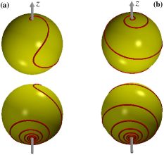
Figure 2: Two spherical pendulum trajectories, shown from perspectives above and below the sphere. In (a), with $h_{a}=2.3$, the sense of the azimuthal rotation changes sign as the trajectory passes from the north to the south pole. In (b), with $h_{a}=5$, the sense of rotation stays the same. In both cases, $\alpha=0.1$, and $v$ and $\omega$ are given by Eq. (16).

Numerical solution of the LLG equation (3) reveals the following surprising behaviour: For initial conditions describing a sufficiently sharp head-to-head domain wall, the evolving profile approaches a traveling wave solution Eq. (4) with specific values of $v$ and $\omega$. The selected velocity and precession frequency depend only on $h_{a}$ and $\alpha$, and not on the initial condition. This is illustrated in Fig. 3, where the initial configuration is taken to be the static (field-free) domain wall profile. At first, the evolution follows the exact precessing solution Goussev et al. (2010). The precessing solution is unstable, however Gou et al. (2011), and after a short time, the new high-field profile emerges, with much higher velocity.

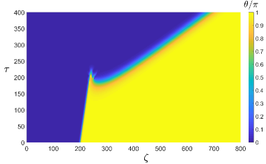
Figure 3: Emergence of high-field profile: the evolution of the polar angle $\theta(\zeta,\tau)=\cos^{-1}(m_{3})$ obtained from numerical solution of the LLG equation (3) with static (field-free) domain wall profile as initial condition. Here $h_{a}=3$ and $\alpha=0.1$.

For scalar PDEs, there is a well-established method for determining the selected velocity of travelling-wave solutions based on the theory of front propagation into unstable states (see, eg, van Saarloos (2003) and references therein). Here, we adapt this method for the vector-valued LLG equation (3). The idea is to linearise the LLG equation in the region of the unstable tail of the profile, ie where $\zeta\gg 1$, and find a frame of reference in which, at long times, the propagating solution is nearly stationary. With

$$\bm{m}=-(\bm{\hat{z}}+i\epsilon(\eta_{1}\bm{\hat{x}}+\eta_{2}\bm{\hat{y}}))+O(\epsilon^{2}),\quad\eta=\eta_{1}+i\eta_{2},$$

the linearised LLG equation for $\eta(\zeta,\tau)$ is given by

$$(1+i\alpha)\dot{\eta}=i\eta^{\prime\prime}+i(h_{a}-1)\eta.$$ (9)

The solution is given explicitly by

$$\eta(\zeta,\tau)=\int\hat{\eta}_{0}(k)e^{i(k\zeta-\Omega(k)\tau)}\,dk,\text{ where}$$ (10)

$$\Omega(k)=-(h_{a}-1-k^{2})/(1+i\alpha).$$ (11)

In a frame moving with velocity $v$ and precessing with frequency $\omega$, the profile appears as $\tilde{\eta}(\zeta,\tau)=\color[rgb]{0,0,0}e^{-i\omega\tau}\eta(\zeta-v\tau,\tau)$, with integral representation

$$\tilde{\eta}(\zeta,\tau)=\int\hat{\eta}_{0}(k)e^{i(kv-\Omega(k)-\omega)\tau}\,e^{ik\zeta}\,dk.$$ (12)

For long times $\color[rgb]{0,0,0}\tau$, the integral in (12) may be evaluated by the method of steepest descent; the contour is deformed through the (complex) saddle point $k_{*}$, characterised by

$$\Omega^{\prime}(k_{*})=v,\ \ \operatorname{Im}k_{*}>0.$$ (13)

Evaluation of (12) yields

$$\tilde{\eta}(\zeta,\tau)\approx\frac{\hat{\eta}_{0}(k_{*})}{(2\pi\Omega^{\prime\prime}(k_{*})\tau)^{1/2}}\,e^{i(k_{*}v-\Omega(k_{*})-\omega)\tau}\,e^{ik_{*}\zeta}.$$ (14)

We choose $v$ and $\omega$ so that $\tilde{\eta}(\zeta,\tau)$ is $\tau$-independent (apart for a diffusive prefactor $\tau^{-1/2}$), ie so that

$$k_{*}v=\Omega(k_{*})-\omega.$$ (15)

With some calculation, Eqs. (11), (13) and (15) yield

$$v=2\left(\frac{h_{a}-1}{1+\alpha^{2}}\right)^{1/2},\quad\omega=2\,\frac{h_{a}-1}{1+\alpha^{2}}.$$ (16)

We note that it is precisely when $v$ and $\omega$ are given by (16) that the roots of (7) with $\sigma=-1$ coincide. This phenemenon is well known for scalar PDEs of reaction-diffusion type, for example the KPP equation Kolmogorov et al. (1937).

Confirmation of the preceding theory is provided in Fig. 4. We solve the LLG equation (3) numerically for a variety of initial conditions, using a finite difference scheme on a uniform rectangular grid, where spatial derivatives are represented by central finite differences with Neumann boundary conditions. A time step is calculated via an explicit fourth-order Runge-Kutta method. In order to exactly maintain the constraint on the magnetization norm, the solution is renormalized after each time step. We determine the (initial-condition-independent) velocity and precession frequency of the emergent profile as functions of $h_{a}$ and of $\alpha$. These are in good agreement with the analytic formulas (16).

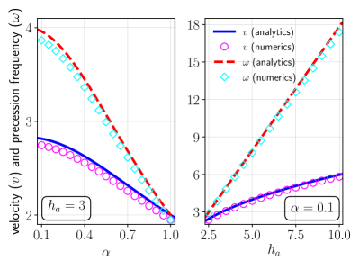
Figure 4: Velocity (circles) and precession frequency (diamonds) of the high-field profile obtained from numerical solution of the LLG equation (3), along with the analytic predictions of Eq. (16), plotted as functions of (a) damping constant $\alpha$ for $h_{a}=3$ and (b) applied field $h_{a}$ for $\alpha=0.1$.

Numerically computed profiles are shown in the Supplemental Material . They coincide with solutions of the ODE (5) with $v$ and $\omega$ given by (16). In particular, the chiralities of the domain wall tails are obtained from (7).

As noted previously, with $h_{a}>1$, the uniform profile $\bm{m}=-\bm{\hat{z}}$ is unstable. It follows that the high-field profile is unstable to perturbations in the region $\zeta\gg 1$, for example due to thermal excitation of spin waves. To estimate the time scale for this instability to set in, we model this region as a cylindrical nanowire of finite length $L\gg\delta_{ex}$, where the exchange length, $\delta_{ex}=\sqrt{A/K}$, is the width of the field-free domain wall. (The estimate turns out to be independent of the choice of $L$.) The magnetisation is governed by the linearised LLG equation (9) with transverse component, $\eta(\zeta,\tau)$, given by (10) but with the $k$-integral replaced by a sum over spin wave modes of wavenumber $k_{j}$, with spin wave amplitudes $\hat{\eta}_{0}(k_{j})$ and (complex) frequencies $\Omega(k_{j})$. The phases $\arg\hat{\eta}_{0}(k_{j})$ are uncorrelated, so that the mean squared amplitude $|\eta|^{2}$ is the sum of the squared amplitudes of the spin waves. We suppose the magnetic field is applied from $\tau=0$ onwards, and let $\tau_{c}$ denote the time required for $|\eta|^{2}$ to equal one.

As a crude approximation, we suppose that only spin waves with wavelengths greater than $\delta_{ex}$ contribute; the number of such spin waves is approximately $L/\delta_{ex}$. Moreover, for these spin waves, we replace $|\hat{\eta}(k_{j})|$ and $\Omega(k_{j})$ by their long wavelength limits $|\hat{\eta}_{0}|$ and $\Omega_{0}$, replacing $k_{j}$ by $k_{0}=1/L$ (more careful calculation does not change the estimate appreciably). We obtain $|\eta(\zeta,\tau)|^{2}\approx(L/\delta_{ex})|\hat{\eta}_{0}|^{2}e^{2\operatorname{Im}\Omega_{0}\tau}$, so that $2\operatorname{Im}\Omega_{0}\tau_{c}\approx\log((\delta_{ex}/L)/|\hat{\eta}_{0}|^{2})$. After time $\tau_{c}$, the domain wall travels a distance (in units of the exchange length)

$$d_{c}=v\tau_{c}=\frac{1}{\alpha}\sqrt{\frac{1+\alpha^{2}}{h_{a}-1}}\log\frac{\delta_{ex}/L}{|\hat{\eta}_{0}|^{2}},$$ (17)

where $v$ is given by (16) and we have used (11) for $\Omega_{0}$.

The initial amplitude $|\hat{\eta}_{0}|$ may be estimated from a simple equipartition argument. The associated spin wave energy is approximately $|\hat{\eta}_{0}|^{2}KSL$, where $S$ is the cross-sectional area of the wire (for long wavelengths, the exchange energy is negligible). At temperature $T$, before the magnetic field is applied, each spin wave mode has energy $k_{B}T$, where $k_{B}$ is Boltzmann’s constant. Thus,

$$|\hat{\eta}_{0}|^{2}=k_{B}T/(KSL).$$ (18)

To estimate $d_{c}$, we take as representative values $A=10^{-11}$ J/m, $M_{s}H_{a}=2K=10^{6}$ J/m³, $S=100$ nm², $T=100$K and $\alpha=0.01$. (For $M_{s}=10^{6}{\rm A/m}$, this corresponds to an applied field strength of 1 Tesla.) In this case, the high-field domain wall propagates for approximately 500 static domain-wall widths before being overtaken by thermal instabilities.

It is interesting to compare the (unscaled) high-field domain wall velocity $V$ in a uniaxial wire with easy-axis anistropy $K$ to the Walker velocity $V_{W}$ for a strongly anisotropic wire with easy-axis anisotropy $K$ and hard-axis anisotropy $K_{2}>K$, For large applied field in the uniaxial case and large $K_{2}$ in the anisotropic case (and weak damping for both),

$$V/V_{W}\sim\sqrt{8M_{s}H_{a}/K_{2}}.$$ (19)

Thus, for $H_{a}$ comparable to $K_{2}/M_{s}$, the high-field domain wall velocity in the uniaxial wire is greater than the Walker velocity in the anisotropic wire.

We have concentrated on the case of uniaxial nanowires. Numerical calculations reveal qualitatively similar behaviour for small nonvanishing hard-axis anisotropy – ie, a new high-field domain wall profile with characteristic velocity and precession frequency. A perturbative analysis can be developed for small $K_{2}>0$.

The dynamics of domain walls in nanowires under small applied fields and currents has been extensively studied. Here we consider the response of a domain wall to an applied magnetic field strong enough to make one of the domains unstable. Naively one might imagine the unstable domain to reorient itself spontaneously and incoherently. Surprisingly, we show that for small transverse anisotropy, there emerges a coherent reorientation, whereby the energetically stable domain grows via the propagation of a travelling and precessing domain wall.

The threshold for the high-field regime is $H_{a}>K/M_{s}$. For an isotropic material such as permalloy, $K\simeq\tfrac{1}{4}\mu_{0}M_{s}^{2}$ Muratov et al. (2017). In particular, for permalloy, $M_{s}\simeq 800\,$kA/m Bain (2001), so that the threshold is given approximately by $\tfrac{1}{4}\mu_{0}M_{s}\simeq 0.25\,$T. We note that early experiments on domain-wall motion in iron-garnet films at applied fields above the anisotropy threshold Logginov and Nepokoichitskii (1982); Ivanov et al. (1983) indicate a sublinear velocity response compatible with (16). Radiation damping at high fields is discussed in a related theoretical work Bar’yakhtar and Ivanov (1982).

The high-field domain wall profile has novel features. Unlike the well-known Walker profile, it is nonplanar with asymmetrical tails comprised of spin-wave trains of different characteristic wavenumbers and helicities. The coherent magnetization switching is eventually overtaken by thermal fluctuations far into the unstable domain, but can persist over length scales of many hundreds of widths of the domain wall. For realistic parameters, the domain wall velocity in the high-field regime can be comparable to or larger than the Walker velocity.

Benguria and Depassier Depassier (2015); Benguria and Depassier (2016) consider the complementary case of strong biaxial anisotropy $K\ll K_{2}$, characteristic of thin ferromagnetic films. There appear transitions (depending on $\alpha$ and $K/K_{2}$) between the Walker solution with velocity $v\sim H_{a}$ and a KPP-type solution (for which one of the domains is necessarily unstable) with $v\sim\sqrt{H_{a}}$. In this regime, the magnetisation is confined to a plane, and the LLG equation reduces to a scalar equation of reaction-diffusion type, for which the theory of unstable front propagation is highly developed (see e.g. van Saarloos (2003)). For the case of near-uniaxial wires considered here, the LLG equation is a vectorial equation; much less is known about unstable front propagation for systems as opposed to scalar equations.

We are grateful to L.P. Ivanov for drawing our attention to References Logginov and Nepokoichitskii (1982)–Bar’yakhtar and Ivanov (1982) and for interesting comments. AG thanks EPSRC for support under grant EP/K024116/1. JMR, VS and SV thank EPSRC for support under grant EP/K02390X/1. JMR and VS thank the Isaac Newton Institute for Mathematical Sciences for support and hospitality during the programme Mathematical Design of New Materials, supported by EPSRC grant number EP/R014604/1. JMR acknowledges support from a Lady Davis Visiting Professorship at Hebrew University and a University Research Fellowship from the University of Bristol.

References

- Tatara and Kohno (2004) G. Tatara and H. Kohno, Phys. Rev. Lett. 92, 086601 (2004).
- Beach et al. (2005) G. S. D. Beach, C. Nistor, C. Knutson, M. Tsoi, and J. L. Erskine, Nat. Mater. 4, 741 (2005).
- Hayashi et al. (2007) M. Hayashi, L. Thomas, C. Rettner, R. Moriya, and S. S. P. Parkin, Nat. Phys. 3, 21 (2007).
- Hayashi et al. (2008) M. Hayashi, L. Thomas, R. Moriya, C. Rettner, and S. S. P. Parkin, Science 320, 209 (2008).
- Thomas et al. (2010) L. Thomas, R. Moriya, C. Rettner, and S. S. Parkin, Science 330, 1810 (2010).
- Braun (2012) H.-B. Braun, Advances in Physics, Advances in Physics 61, 1 (2012).
- Hellman et al. (2017) F. Hellman, A. Hoffmann, Y. Tserkovnyak, G. S. D. Beach, E. E. Fullerton, C. Leighton, A. H. MacDonald, D. C. Ralph, D. A. Arena, H. A. Dürr, P. Fischer, J. Grollier, J. P. Heremans, T. Jungwirth, A. V. Kimel, B. Koopmans, I. N. Krivorotov, S. J. May, A. K. Petford-Long, J. M. Rondinelli, N. Samarth, I. K. Schuller, A. N. Slavin, M. D. Stiles, O. Tchernyshyov, A. Thiaville, and B. L. Zink, Reviews of Modern Physics 89, 025006 (2017).
- Allwood et al. (2005) D. A. Allwood, G. Xiong, C. C. Faulkner, D. Atkinson, D. Petit, and R. P. Cowburn, Science 309, 1688 (2005).
- Parkin et al. (2008) S. S. P. Parkin, M. Hayashi, and L. Thomas, Science 320, 190 (2008).
- Yan et al. (2011) M. Yan, C. Andreas, A. Kákay, F. García-Sánchez, and R. Hertel, Appl. Phys. Lett. 99, 122505 (2011).
- Goussev et al. (2014) A. Goussev, J. M. Robbins, and V. Slastikov, Europhys. Lett. 105, 67006 (2014).
- Depassier (2014) M. Depassier, Europhys. Lett. 108, 2 (2014).
- Gaididei et al. (2014) Y. Gaididei, V. P. Kravchuk, and D. D. Sheka, Phys. Rev. Lett. 112, 257203 (2014).
- Gaididei et al. (2017) Y. Gaididei, A. Goussev, V. P. Kravchuk, O. V. Pylypovskyi, J. M. Robbins, D. D. Sheka, V. Slastikov, and S. Vasylkevych, J. Phys. A: Math. Theor. 50, 385401 (2017).
- Boulle et al. (2013) O. Boulle, S. Rohart, L. D. Buda-Prejbeanu, E. Jué, I. M. Miron, S. Pizzini, J. Vogel, G. Gaudin, and A. Thiaville, Physical Review Letters 111, 217203 (2013).
- Tatara et al. (2008) G. Tatara, H. Kohno, and J. Shibata, Physics Reports 468, 213 (2008).
- Thiaville and Nakatani (2006) A. Thiaville and Y. Nakatani, in Spin Dynamics in Confined Magnetic Structures III, Topics in applied physics, Vol. 101 (Springer, 2006) pp. 161–205.
- Goussev et al. (2013) A. Goussev, R. G. Lund, J. Robbins, V. Slastikov, and C. Sonnenberg, Proc. R. Soc. Lond. A 469, 20130308 (2013).
- Depassier (2015) M. C. Depassier, Europhys. Lett. 111, 27005 (2015).