Nonlinear saturation and oscillations of collisionless zonal flows

Abstract

In homogeneous drift-wave (DW) turbulence, zonal flows (ZFs) can be generated via a modulational instability (MI) that either saturates monotonically or leads to oscillations of the ZF energy at the nonlinear stage. This dynamics is often attributed as the predator–prey oscillations induced by ZF collisional damping; however, similar dynamics is also observed in collisionless ZFs, in which case a different mechanism must be involved. Here, we propose a semi-analytic theory that explains the transition between the oscillations and saturation of collisionless ZFs within the quasilinear Hasegawa–Mima model. By analyzing phase-space trajectories of DW quanta (driftons) within the geometrical-optics (GO) approximation, we argue that the parameter that controls this transition is $N\sim\gamma_{{\rm MI}}/\omega_{{\rm DW}}$, where $\gamma_{{\rm MI}}$ is the MI growth rate and $\omega_{{\rm DW}}$ is the linear DW frequency. We argue that at $N\ll 1$, ZFs oscillate due to the presence of so-called passing drifton trajectories, and we derive an approximate formula for the ZF amplitude as a function of time in this regime. We also show that at $N\gtrsim 1$, the passing trajectories vanish and ZFs saturate monotonically, which can be attributed to phase mixing of higher-order sidebands. A modification of $N$ that accounts for effects beyond the GO limit is also proposed. These analytic results are tested against both quasilinear and fully-nonlinear simulations. They also explain the earlier numerical results by Connaughton et al. [J. Fluid Mech. 654, 207 (2010)] and Gallagher et al. [Phys. Plasmas 19, 122115 (2012)] and offer a revised perspective on what the control parameter is that determines the transition from the oscillations to saturation of collisionless ZFs.

I Introduction

Zonal flows (ZFs) are banded sheared flows that can spontaneously emerge from drift-wave (DW) turbulence in magnetized plasmas (Lin98, ; Diamond05, ; Rogers00, ; Jenko00, ) and, similarly, from Rossby-wave turbulence in the atmospheres of rotating planets (Vasavada05, ). They are considered important as regulators of turbulent transport and thus have been studied actively by many researchers. One mechanism of the ZF generation is the secondary (or zonostrophic) instability (Rogers00, ; Smolyakov00a, ; Smolyakov00b, ; Strintzi07, ; Srinivasan2012, ; Parker2013, ; Parker2014, ; Parker14Thesis, ; St-Onge17a, ; Marston16, ), and the modulational instability (MI) as a special case when the DW is monochromatic (Qi19, ; Chen00, ; Connaughton10, ; Gallagher12, ; Connaughton15, ; Champeaux01, ; Koshkarov16, ; Lashkin08, ; Jenko06, ; Shukla02, ; Manfredi01, ; Lashmore-Davies01, ; Gill74, ; Mahanti81, ; St-Onge17b, ). The linear stage of the MI is generally understood, but the dynamics of ZFs at the nonlinear stage is not sufficiently explored. Some progress in this area has been made by applying quasilinear (QL) models (Sec. II.4), such as the second-order cumulant expansion theory (CE2) (Srinivasan2012, ; Parker2013, ; Parker2014, ; Parker14Thesis, ; St-Onge17a, ; Marston16, ), or the stochastic structural stability theory (SSST) (Constantinou18, ; Farrell07, ; Bakas15, ); however, those are not particularly intuitive. A more intuitive paradigm was proposed based on a simpler QL model known as the wave-kinetic equation (WKE) (Smolyakov00a, ; Smolyakov00b, ; Ruiz16, ; Ruiz18, ; Zhu18a, ; Zhu18b, ; Parker16, ; Smolyakov99, ; Kaw2001, ). The WKE treats DW turbulence as a collection of DW quanta (“driftons”), for which the ZF velocity serves as a collective field. Then, the ZF–DW interactions can be viewed as the predator–prey dynamics, which can result in either monotonic or oscillatory energy exchange between the ZFs and DWs (Malkov01, ; Miki12, ; Diamond94, ; Kim03, ; Berionni11, ). Such dynamics is indeed observed in simulations (Kobayashi15, ). However, the existing paradigm substantially relies on collisional damping of ZFs, whereas simulations indicate that nonlinear saturation and oscillations are also possible when the ZF is collisionless (Connaughton10, ; Gallagher12, ; Manfredi01, ; Lashmore-Davies01, ; Mahanti81, ). This leads to the question of how this dynamics can be explained within a collisionless theory.

Here, we propose a semi-analytic theory that explains the transition between the oscillations and saturation of collisionless ZFs within the QL Hasegawa–Mima model. By analyzing phase-space trajectories of DW quanta (driftons) within the geometrical-optics (GO) approximation, we argue that the parameter that controls this transition is $N\sim\gamma_{{\rm MI}}/\omega_{{\rm DW}}$, where $\gamma_{{\rm MI}}$ is the MI growth rate and $\omega_{{\rm DW}}$ is the linear DW frequency. We argue that at $N\ll 1$, ZFs oscillate due to the presence of so-called passing drifton trajectories, and we derive an approximate formula for the ZF amplitude as a function of time in this regime. In doing so, we also extend the applicability of the popular “four-mode truncation” (4MT) model (Chen00, ; Connaughton10, ; Gallagher12, ; Connaughton15, ; Champeaux01, ; Koshkarov16, ; Lashkin08, ; Jenko06, ; Shukla02, ; Manfredi01, ; Lashmore-Davies01, ; Mahanti81, ; Gill74, ; St-Onge17b, ), which is commonly used for the linear stage, to nonlinear ZF–DW interactions. We also show that at $N\gtrsim 1$, the passing trajectories vanish and ZFs saturate monotonically, which can be attributed to phase mixing of higher-order sidebands. A modification of $N$ that accounts for effects beyond the GO limit is also proposed. These analytic results are tested against both QL and fully-nonlinear (NL) simulations. They also explain the earlier numerical results by Connaughton et al. (Connaughton10, ) and Gallagher et al. (Gallagher12, ) and offer a revised perspective on what the control parameter is that determines the transition from oscillations to saturation of collisionless ZFs.

Our paper is organized as follows. In Sec. II, we introduce the basic equations, including the Hasegawa–Mima equation, the 4MT, the QL approximation, the Wigner function, and the WKE that we use later on. In Sec. III, we discuss the nonlinear stage of the MI using both the 4MT description and the WKE, and we also propose our control parameter $N$. In Sec. IV, we compare our results with those in Refs (Connaughton10, ; Gallagher12, ). In Sec. VI we summarize our main conclusions.

II Basic equations

II.1 Hasegawa–Mima equation

Both electrostatic DW turbulence in plasmas and Rossby-wave turbulence in the atmospheres of rotating planets are often modeled by the Hasegawa–Mima equation (HME) (Hasegawa77, ):

$$\frac{\partial w}{\partial t}+(\hat{\boldsymbol{z}}\times\nabla\varphi)\cdot\nabla w+\beta\,\frac{\partial\varphi}{\partial x}=0,$$ (1)

$$w=(\nabla^{2}-L_{{\rm D}}^{-2}\hat{\alpha})\varphi.$$ (2)

(In geophysics, it is also known as the Obukhov–Charney equation (DolzhanskyBook, ).) Here, the geophysics coordinate convention is used to simplify comparisons with the earlier relevant studies (Sec. V). The HME describes wave turbulence on a two-dimensional plane $(x,y)$, where ZFs develop along the $x$-direction, and $\nabla^{2}\doteq\partial_{x}^{2}+\partial_{y}^{2}$ is the Laplacian. In the plasma-physics context, the system is assumed to be immersed in a uniform magnetic field along the $z$ axis, the plasma is assumed to have a constant density gradient along the $y$ axis, $\beta$ is a scalar constant proportional to this gradient, $L_{{\rm D}}$ is the ion-sound radius, and $\varphi$ is the perturbation of the electrostatic potential. In the geophysical context, the constant $\beta$ is proportional to the latitudinal gradient of the vertical rotation frequency, $L_{{\rm D}}$ is the deformation radius, and $\varphi$ is the stream function.

The operator $\hat{\alpha}$ is an identity operator in the original HME (oHME). The so-called modified HME (mHME), which is also known as “generalized” (Ruiz16, ; Krommes00, ) or “extended” HME (Connaughton15, ; Gallagher12, ), uses $\hat{\alpha}f\doteq f-\langle f\rangle$, where $f=f(x,y,t)$ is any field quantity and $\langle f\rangle\doteq\int_{0}^{L_{x}}fdx/L_{x}$ denotes the zonal average, where $L_{x}$ is the system length in the $x$-direction. (For more details, see, for example, Ref. (St-Onge17b, ; Hammett93, ).) Below, we consider both the oHME and mHME and treat them on the same footing.

II.2 Fourier decomposition and the 4MT

It is common to approach the dynamics of $\varphi$ in the Fourier representation, $\varphi=\sum_{\boldsymbol{k}}\varphi_{\boldsymbol{k}}(t)\exp(i\boldsymbol{k}\cdot\boldsymbol{x})$, where $\boldsymbol{k}=(k_{x},k_{y})$ and $\boldsymbol{x}=(x,y)$. This leads to the following equation for $\varphi_{\boldsymbol{k}}$:

$$\frac{\partial\varphi_{\boldsymbol{k}}}{\partial t}=i\omega_{\boldsymbol{k}}\varphi_{\boldsymbol{k}}+\frac{1}{2}\sum_{\boldsymbol{k}_{1},\boldsymbol{k}_{2}}T(\boldsymbol{k},\boldsymbol{k}_{1},\boldsymbol{k}_{2})\varphi_{\boldsymbol{k}_{1}}\varphi_{\boldsymbol{k}_{2}}\delta_{\boldsymbol{k},\boldsymbol{k}_{1}+\boldsymbol{k}_{2}}.$$ (3)

Here, $\delta_{\boldsymbol{k},\boldsymbol{k}_{1}+\boldsymbol{k}_{2}}$ equals one only if $\boldsymbol{k}=\boldsymbol{k}_{1}+\boldsymbol{k}_{2}$ and is zero otherwise,

$$\omega_{\boldsymbol{k}}\doteq-\frac{\beta k_{x}}{k_{{\rm D}}^{2}}$$ (4)

is the linear DW frequency, and

$$T(\boldsymbol{k},\boldsymbol{k}_{1},\boldsymbol{k}_{2})\doteq-\frac{k_{1,{\rm D}}^{2}-k_{2,{\rm D}}^{2}}{k_{{\rm D}}^{2}}\,(\boldsymbol{k}_{1}\times\boldsymbol{k}_{2})\cdot\hat{\boldsymbol{z}}$$ (5)

are the coefficients that govern the nonlinear mode coupling. Also,

$$k_{{\rm D}}^{2}\doteq|\boldsymbol{k}|^{2}+L_{{\rm D}}^{-2}\alpha_{\boldsymbol{k}},$$ (6)

and $k_{n,{\rm D}}^{2}$ (where $n=1,2$) are similarly defined as

$$k_{n,{\rm D}}^{2}\doteq|\boldsymbol{k}_{n}|^{2}+L_{{\rm D}}^{-2}\alpha_{\boldsymbol{k}_{n}}.$$ (7)

And finally, $\alpha_{\boldsymbol{k}}$ is the Fourier representation of the operator $\hat{\alpha}$; namely, for the oHME $\alpha_{\boldsymbol{k}}$ is unity, and for the mHME $\alpha_{\boldsymbol{k}}$ equals zero if $k_{x}=0$ and equals unity if $k_{x}\neq 0$.

It is also common to introduce the 4MT, which is a truncation of the system (3) that retains only four Fourier harmonics, namely, those with wave vectors $\boldsymbol{p}$, $\boldsymbol{q}$, and $\boldsymbol{p}_{\pm}\doteq\boldsymbol{p}\pm\boldsymbol{q}$. (Since $\varphi$ is real, one has $\varphi_{-\boldsymbol{k}}=\varphi_{\boldsymbol{k}}^{*}$; hence, the harmonics with wave vectors $-\boldsymbol{p}$, $-\boldsymbol{q}$, and $-\boldsymbol{p}_{\pm}$ are included too.) Then, for $\Phi_{\boldsymbol{k}}\doteq\varphi_{\boldsymbol{k}}\exp(-i\omega_{\boldsymbol{k}}t)$, Eq. (3) gives

$$\partial_{t}\Phi_{\boldsymbol{p}}=T(\boldsymbol{p},\boldsymbol{q},\boldsymbol{p}_{-})\Phi_{\boldsymbol{q}}\Phi_{\boldsymbol{p}_{-}}e^{i\Delta_{-}t}$$

$$+T(\boldsymbol{p},-\boldsymbol{q},\boldsymbol{p}_{+})\Phi_{\boldsymbol{q}}^{*}\Phi_{\boldsymbol{p}_{+}}e^{i\Delta_{+}t},$$ (8a)

$$\partial_{t}\Phi_{\boldsymbol{q}}=T(\boldsymbol{q},\boldsymbol{p},-\boldsymbol{p}_{-})\Phi_{\boldsymbol{p}}\Phi_{\boldsymbol{p}_{-}}^{*}e^{-i\Delta_{-}t}$$

$$+T(\boldsymbol{q},-\boldsymbol{p},\boldsymbol{p}_{+})\Phi_{\boldsymbol{p}}^{*}\Phi_{\boldsymbol{p}_{+}}e^{i\Delta_{+}t},$$ (8b)

$$\partial_{t}\Phi_{\boldsymbol{p}_{-}}=T(\boldsymbol{p}_{-},\boldsymbol{p},-\boldsymbol{q})\Phi_{\boldsymbol{p}}\Phi_{\boldsymbol{q}}^{*}e^{-i\Delta_{-}t},$$ (8c)

$$\partial_{t}\Phi_{\boldsymbol{p}_{+}}=T(\boldsymbol{p}_{+},\boldsymbol{p},\boldsymbol{q})\Phi_{\boldsymbol{p}}\Phi_{\boldsymbol{q}}e^{-i\Delta_{+}t},$$ (8d)

where $\Delta_{\pm}=\omega_{\boldsymbol{p}}\pm\omega_{\boldsymbol{q}}-\omega_{\boldsymbol{p}_{\pm}}$.

II.3 Modulational instability

Suppose a perturbation on a primary wave $\Phi_{\boldsymbol{p}}=\Phi_{0}$,

$$\left(\begin{array}[]{c}\Phi_{\boldsymbol{p}}\\ \Phi_{\boldsymbol{q}}\\ \Phi_{\boldsymbol{p}_{+}}\\ \Phi_{\boldsymbol{p}_{-}}\end{array}\right)=\left(\begin{array}[]{c}\Phi_{0}\\ 0\\ 0\\ 0\end{array}\right)+\varepsilon\left(\begin{array}[]{c}0\\ A_{\boldsymbol{q}}e^{-i\Omega_{\boldsymbol{q}}t}\\ A_{\boldsymbol{p}_{+}}e^{-i\Omega_{\boldsymbol{p}_{+}}t}\\ A_{\boldsymbol{p}_{-}}e^{-i\Omega_{\boldsymbol{p}_{-}}t}\end{array}\right),$$ (21)

where $\varepsilon$ is small. Then, the linearized Eq. (8) gives $\Omega_{\boldsymbol{p}\pm}=\Delta_{\pm}\pm\Omega_{\boldsymbol{q}}$ together with the following dispersion relation:

$$\Omega_{\boldsymbol{q}}+\frac{|\Phi_{0}|^{2}T(\boldsymbol{q},-\boldsymbol{p},\boldsymbol{p}_{+})T(\boldsymbol{p}_{+},\boldsymbol{q},\boldsymbol{p})}{\Delta_{+}+\Omega_{\boldsymbol{q}}}\\ -\frac{|\Phi_{0}|^{2}T(\boldsymbol{q},-\boldsymbol{p}_{-},\boldsymbol{p})T(\boldsymbol{p}_{-},-\boldsymbol{q},\boldsymbol{p})}{\Delta_{-}-\Omega_{\boldsymbol{q}}}=0.$$ (22)

(The derivation can be found, for example, in Ref. (Gallagher12, ).) This equation can have a complex solution for $\Omega_{\boldsymbol{q}}$ with $\text{Im}\,\Omega_{\boldsymbol{q}}>0$, which signifies the presence of the MI. As shown in Refs. (Connaughton10, ; Gill74, ), the 4MT is indeed often a good approximation at the linear stage of the MI.

In the following, we restrict our discussions to the case when $\boldsymbol{p}=(p,0)$ and $\boldsymbol{q}=(0,q)$. In this case, $\omega_{\boldsymbol{q}}=0$ and

$$\Delta_{\pm}\equiv\Delta\doteq\frac{\beta pq^{2}}{p_{{\rm D}}^{2}(p_{{\rm D}}^{2}+q^{2})},$$ (23)

where

$$p_{{\rm D}}^{2}\doteq L_{{\rm D}}^{-2}+p^{2}.$$ (24)

Then, one finds that $\Omega_{\boldsymbol{q}}^{2}$ is real, and hence the MI has a positive growth rate $\gamma_{{\rm MI}}$ if $\Omega_{\boldsymbol{q}}^{2}$ is negative; namely, $\gamma_{{\rm MI}}^{2}\doteq-\Omega_{\boldsymbol{q}}^{2}$, which can be explicitly written as

$$\gamma_{{\rm MI}}^{2}=\frac{2|\Phi_{0}|^{2}p^{2}q^{2}}{(1+\alpha L_{{\rm D}}^{-2}q^{-2})}\,\frac{\delta^{\prime}-1}{\delta+1}-\Delta^{2}.$$ (25)

Here,

$$\delta\doteq\frac{p_{{\rm D}}^{2}}{q^{2}},\quad\delta^{\prime}\doteq\frac{p_{{\rm D}}^{2}-\alpha L_{{\rm D}}^{-2}}{q^{2}},$$ (26)

with $\alpha=1$ for the oHME and $\alpha=0$ for the mHME. Notably, this implies that the mHME gives much larger growth rates than the oHME does. Also, a necessary condition for the modulation to be unstable is $\delta^{\prime}>1$, which requires

$$q^{2}<p_{{\rm D}}^{2}-\alpha L_{{\rm D}}^{-2}.$$ (27)

II.4 Quasilinear approximation

In order to describe the nonlinear stage of the MI analytically, we proceed as follows. Let us decompose the field quantities into the zonal-averaged part and the fluctuation part, $f=\langle f\rangle+\tilde{f}$. Then, Eqs. (1) and (2) become (Parker14Thesis, )

$$\frac{\partial\tilde{w}}{\partial t}+U\,\frac{\partial\tilde{w}}{\partial x}+\left[\beta-\left(\frac{\partial^{2}}{\partial y^{2}}-\alpha L_{{\rm D}}^{-2}\right)U\right]\frac{\partial\tilde{\varphi}}{\partial x}=f_{{\rm NL}},$$ (28)

$$\left[1-\alpha L_{{\rm D}}^{-2}\left(\frac{\partial}{\partial y}\right)^{-2}\right]\frac{\partial U}{\partial t}=-\frac{\partial}{\partial y}\langle\tilde{v}_{x}\tilde{v}_{y}\rangle.$$ (29)

Here, $U(y,t)\doteq-\partial_{y}\langle\varphi\rangle$ is the ZF velocity, $\tilde{\boldsymbol{v}}\doteq\hat{\boldsymbol{z}}\times\nabla\tilde{\varphi}$ is the fluctuation velocity, $\partial_{y}^{-2}$ is an operator that in the wave-vector (Fourier) representation is simply a multiplication by $-k_{y}^{-2}$, and $f_{{\rm NL}}\doteq\tilde{\boldsymbol{v}}\cdot\nabla\tilde{w}-\langle\tilde{\boldsymbol{v}}\cdot\nabla\tilde{w}\rangle$ describes self-interactions of DWs, or eddy–eddy interactions. We shall simplify the problem by ignoring these interactions, i.e., by adopting $f_{{\rm NL}}=0$. This is the commonly-used QL approximation, which often yields an adequate description of ZF–DW interactions (Parker14Thesis, ). (We shall also discuss the applicability of this approximation in Sec. IV.2). Notably, once the QL approximation is adopted, the 4MT model becomes the exact description of the linear MI.

We also assume, for simplicity, that the ZF is sinusoidal and non-propagating (assuming $\gamma_{{\rm MI}}$ is real),

$$U=u(t)\cos qy,$$ (30)

where for clarity we choose the origin on the $y$ axis such that $y=0$ corresponds to the maximum of $U$. (Propagating zonal structures are studied in detail in our Ref. (soliton, ).) The assumption of spatially-monochromatic ZF holds approximately if the ZF’s second and higher harmonics do not outpace the fundamental harmonic during the linear MI. Hence, the ansatz (30) implies that the value of $q$ is close to the one that maximizes $\gamma_{{\rm MI}}$. Then, the DW field can be represented as $\tilde{\varphi}={\rm Re}\sum_{m=-\infty}^{\infty}\varphi_{m}(t)\exp(ipx+imqy)$, where $\varphi_{0}(t=0)=\Phi_{0}$ is the primary-wave amplitude, and the DW equation (28) becomes

$$\frac{\partial\varphi_{m}}{\partial t}=i\omega_{m}\varphi_{m}+\frac{ipu}{2}\left(\frac{q^{2}+\alpha L_{{\rm D}}^{-2}-k_{m+1,{\rm D}}^{2}}{k_{m,{\rm D}}^{2}}\right)\varphi_{m+1}\\ +\frac{ipu}{2}\left(\frac{q^{2}+\alpha L_{{\rm D}}^{-2}-k_{m-1,{\rm D}}^{2}}{k_{m,{\rm D}}^{2}}\right)\varphi_{m-1},$$ (31)

where

$$\omega_{m}\doteq-\frac{\beta p}{k_{m,{\rm D}}^{2}},\quad k_{m,{\rm D}}^{2}\doteq p_{{\rm D}}^{2}+(mq)^{2}.$$ (32)

Note that the definition of $k_{m,D}$ is consistent with that given by Eq. (7).

II.5 Wigner function and WKE

Equation (31) describes the mode-coupling among different Fourier modes of DWs due to the ZF. Now, we seek to interpret this equation in terms of the drifton phase-space dynamics. Consider the zonal-averaged Wigner function of DWs,

$$W(y,\boldsymbol{k},t)=\int d^{2}se^{-i\boldsymbol{k}\cdot\boldsymbol{s}}\left<\tilde{w}(\boldsymbol{x}+\frac{\boldsymbol{s}}{2},t)\tilde{w}(\boldsymbol{x}-\frac{\boldsymbol{s}}{2},t)\right>.$$ (33)

It can be understood as the spectral representation of the DW two-point correlation function, such as the one used in the CE2. It can also be viewed as the quasiprobability of the drifton distribution in the $(y,\boldsymbol{k})$ space, where the prefix “quasi” reflects the fact that $W$ is not necessarily positive-definite. That said, it becomes positive-definite in the GO limit defined as (i) $\alpha L_{{\rm D}}^{-2}+q^{2}\ll L_{{\rm D}}^{-2}+p^{2}$ and (ii) $\partial_{k_{y}}W\ll q^{-1}W$, when it can be considered as the true distribution function of driftons (Cartwright76, ). Then, the Wigner function can be shown to satisfy the following partial differential equation (Ruiz16, ; Parker16, ):

$$\partial_{t}W(y,\boldsymbol{k},t)=\{\mathcal{H},W\}+2\Gamma W.$$ (34)

Here, $\{\cdot,\cdot\}$ is the Poisson bracket,

$$\{A,B\}\doteq\frac{\partial A}{\partial\boldsymbol{x}}\cdot\frac{\partial B}{\partial\boldsymbol{k}}-\frac{\partial A}{\partial\boldsymbol{k}}\cdot\frac{\partial B}{\partial\boldsymbol{x}},$$ (35)

and the functions $\mathcal{H}$ and $\Gamma$ can be interpreted as the drifton Hamiltonian and the drifton dissipation rate, respectively. Specifically, they are given by (Ruiz16, ; Zhu18b, )

$$\mathcal{H}(y,\boldsymbol{k},t)=k_{x}\left[u(t)\cos qy-\frac{\beta+(q^{2}+\alpha L_{{\rm D}}^{-2})u(t)\cos qy}{k_{{\rm D}}^{2}}\right],$$

$$\Gamma(y,\boldsymbol{k},t)=-\frac{k_{x}k_{y}q(q^{2}+\alpha L_{{\rm D}}^{-2})u(t)\sin qy}{k_{{\rm D}}^{4}}.$$ (36)

Equation (34) is the WKE that describes the phase-space dynamics of driftons (DW quanta). They obey Hamilton’s equations and move on constant-$\mathcal{H}$ surfaces in the phase-space $(y,k_{y})$ if the ZF is stationary. (The $x$-momentum $k_{x}=p$ serves only as a parameter.) In the GO limit, $\Gamma$ is small and unimportant for the discussions below. However, in general, keeping $\Gamma$ is necessary to ensure that the WKE preserves the conservation of the fundamental integrals of the HME (Parker16, ).

II.6 Evolution of $\boldsymbol{W}$ beyond the GO approximation

Beyond the GO approximation, the Wigner function satisfies a pseudo-differential equation known as the Wigner–Moyal equation (Ruiz16, ). But here, we use a somewhat different formulation. Following the procedure in Ref. (Ruiz16, ), we consider the spectrum of $W$,

$$W_{\lambda}(\boldsymbol{k},t)\doteq\int W(y,\boldsymbol{k},t)\exp(-i\lambda y)dy,$$ (37)

which is a function in the double-momentum space $(\lambda,k_{y})$. Then, Eq. (31) is transformed into

$$\partial_{t}W_{\lambda}(p,k_{y},t)=i\beta p\left(\frac{1}{\kappa_{+\lambda}^{2}}-\frac{1}{\kappa_{-\lambda}^{2}}\right)W_{\lambda,0}\\ -\frac{iup}{2}\,Q_{\lambda-2q}W_{\lambda-q,-q}+\frac{iup}{2}\,Q_{2q-\lambda}W_{\lambda-q,+q}\\ -\frac{iup}{2}\,Q_{\lambda+2q}W_{\lambda+q,+q}+\frac{iup}{2}\,Q_{-2q-\lambda}W_{\lambda+q,-q},$$ (38)

where we introduced

$$W_{a,b}\doteq W_{a}\left(p,k_{y}+\frac{b}{2},t\right),\quad\kappa_{a}^{2}\doteq p_{{\rm D}}^{2}+\left(k_{y}+\frac{a}{2}\right)^{2},$$

and

$$Q_{a}\doteq 1-\frac{\alpha L_{{\rm D}}^{-2}+q^{2}}{\kappa_{a}^{2}}.$$ (39)

Equation (38) is equivalent to Eq. (31), but describes the dynamics in the double-momentum space. The DW momentum flux can also be expressed through $W_{\lambda}$, whose gradient drives the Fourier component of the ZF, $U_{\lambda=q}\doteq\pi u(t)$. Specifically, from Eq. (29), the following equation is obtained:

$$\frac{\partial U_{q}}{\partial t}=\frac{i}{(1+\alpha L_{{\rm D}}^{-2}q^{-2})}\int\frac{d^{2}k}{(2\pi)^{2}}\frac{k_{x}k_{y}q}{\kappa_{+q}^{2}\kappa_{-q}^{2}}W_{q}(\boldsymbol{k},t).$$ (40)

III Nonlinear stage of the modulation instability

III.1 4MT description

In order to describe the nonlinear stage of the MI, let us first consider this instability within the 4MT model. We shall show that the 4MT has an exact analytic solution that not only gives the linear growth rate (25), but also predicts the reversal of the ZF growth. We shall also propose a toy-model modification of the 4MT that qualitatively explains the transition from ZF oscillations to saturation.

For the MI, the initial condition is $\tilde{\varphi}(\boldsymbol{x},t=0)=\Phi_{0}\exp(ipx)+{\rm c.c.}$, which corresponds to a delta function in the double-momentum space [Eq. (33)],

$$W_{\lambda}(\boldsymbol{k},t=0)=a_{0}\delta(\lambda)\delta(k_{y})[\delta(k_{x}-p)+\delta(k_{x}+p)],$$ (41)

$$a_{0}\doteq 8\pi^{3}(L_{{\rm D}}^{-2}+p^{2})^{2}|\Phi_{0}|^{2}.$$ (42)

According to Eq. (38), $W_{\lambda}(\boldsymbol{k},t)$ remains delta-shaped also at $t>0$, so we search it in the form

$$W_{\lambda}(p,k_{y},t)=\sum_{m,n}\bar{W}_{m,n}(t)\delta(\lambda-mq)\delta(k_{y}-nq/2),$$ (43)

where the factor $\delta(k_{x}-p)$ is omitted, and $W_{\lambda}(-\boldsymbol{k},t)=W_{\lambda}(\boldsymbol{k},t)$. The 4MT model (Sec. II.2) corresponds to keeping the following nine peaks:

$$\bar{W}_{0,0}\doteq a(t),\quad\bar{W}_{\pm 2,0}=\bar{W}_{0,\pm 2}\doteq d(t),$$

$$\bar{W}_{1,\pm 1}\doteq b(t)\pm ic(t),\quad\bar{W}_{-1,\pm 1}\doteq b(t)\mp ic(t).$$

Here, $a$, $b$, $c$, and $d$ are real, and the initial value of $a(t)$ is $a_{0}$. Using Eq. (38), one obtains

$$\dot{a}=2puc\,\frac{\delta^{\prime}}{1+\delta},\quad\dot{b}=\Delta c,\quad\dot{d}=puc\,\frac{1-\delta^{\prime}}{\delta},$$

$$\dot{c}=-\Delta b+\frac{pua}{2}\,\frac{1-\delta^{\prime}}{\delta}+pud\,\frac{\delta^{\prime}}{1+\delta}.$$ (44)

Here, $\Delta$, $\delta$, and $\delta^{\prime}$ are defined by Eqs. (23) and (26). Also, the ZF amplitude is governed by [Eq. (40)]

$$\dot{u}=-\frac{pq^{2}c}{\epsilon p_{{\rm D}}^{2}(p_{{\rm D}}^{2}+q^{2})},$$ (45)

where we introduced

$$\epsilon\doteq 2\pi^{3}(1+\alpha L_{{\rm D}}^{-2}q^{-2}).$$ (46)

Note that DWs with $k_{x}=p$ and $k_{x}=-p$ contribute equally to $\dot{u}$.

In the following, we simplify the above equations and obtain the time-evolution of $u$. First, notice that

$$\frac{\dot{d}}{\dot{a}}=\frac{(1-\delta^{\prime})(1+\delta)}{2\delta\delta^{\prime}}.$$ (47)

Thus, $d$ can be expressed through $a$:

$$d=\frac{(1-\delta^{\prime})(1+\delta)}{2\delta\delta^{\prime}}(a-a_{0}),$$ (48)

where $a_{0}$ is given by Eq. (42). Next, we introduce dimensionless variables

$$\tau=t/T,\quad\bar{a}=a/A,\quad\bar{b}=b/B,\quad\bar{c}=c/C,\quad\bar{u}=u/V,$$

where we choose $B=C=\beta\epsilon V$ and

$$T=\frac{q^{2}\delta(\delta+1)}{\beta p},\,A=\frac{\beta^{2}\epsilon}{q^{2}(\delta+1)(\delta^{\prime}-1)},\,V=\sqrt{\frac{A}{2\epsilon q^{2}\delta\delta^{\prime}}}.$$

Then, Eqs. (44) and (45) become

$$\frac{d\bar{a}}{d\tau}=\bar{u}\bar{c},\quad\frac{d\bar{u}}{d\tau}=-\bar{c},$$

$$\frac{d\bar{b}}{d\tau}=\bar{c},\quad\frac{d\bar{c}}{d\tau}=-\bar{b}-\left(\bar{a}-\frac{\bar{a}_{0}}{2}\right)\bar{u},$$ (49)

where $\bar{a}_{0}=a_{0}/A$. This leads to

$$\frac{d^{3}\bar{u}}{d\tau^{3}}=-\frac{d^{2}\bar{c}}{d\tau^{2}}=\frac{d\bar{b}}{d\tau}+\left(\bar{a}-\frac{\bar{a}_{0}}{2}\right)\frac{d\bar{u}}{d\tau}+\frac{d\bar{a}}{d\tau}u\\ =-\left[1-\left(\bar{a}-\frac{\bar{a}_{0}}{2}\right)\right]\frac{d\bar{u}}{d\tau}-\left(-\frac{d\bar{a}}{d\tau}u\right)=-\frac{d}{d\tau}(\bar{f}\bar{u}),$$

where

$$\bar{f}\doteq 1-\left(\bar{a}-\frac{\bar{a}_{0}}{2}\right).$$ (50)

Assuming infinitesimally small initial $\bar{u}$, we have

$$\frac{d^{2}\bar{u}}{d\tau^{2}}+\bar{f}\bar{u}=0.$$ (51)

Finally, since

$$\frac{d\bar{f}}{d\tau}=-\frac{d\bar{a}}{d\tau}=-\bar{u}\bar{c}=\frac{1}{2}\frac{d(\bar{u}^{2})}{d\tau},$$ (52)

one has that $\bar{f}-\bar{u}^{2}/2$ is conserved; namely,

$$\bar{f}-\frac{\bar{u}^{2}}{2}=-g^{2}\doteq 1-\frac{\bar{a}_{0}}{2}$$ (53)

is a constant. (Having $g^{2}<0$ is possible but does not lead to an instability; see below.) Hence, we obtain that $\bar{u}$ satisfies a nonlinear-oscillator equation

$$\frac{d^{2}\bar{u}}{d\tau^{2}}=-\frac{d\Theta}{d\bar{u}},\quad\Theta(\bar{u})\doteq-\frac{g^{2}\bar{u}^{2}}{2}+\frac{\bar{u}^{4}}{8}.$$ (54)

The effective potential $\Theta(\bar{u})$ is plotted in Fig. 1(a). (A small nonzero initial value of $\bar{u}$ causes a slight alteration of $\Theta$, but the qualitative picture remains the same.) The steady-state solution $\bar{u}=0$ is unstable if $g^{2}>0$, which signifies the presence of a linear instability (namely, the MI) with the growth rate

$$\gamma_{{\rm MI}}^{2}=\frac{g^{2}}{T^{2}}=\frac{1}{T^{2}}\left(\frac{a_{0}}{2A}-1\right),$$ (55)

which is in agreement with Eq. (25). Beyond the linear regime, i.e., when $\bar{u}^{4}$ is no longer negligible, Eq. (54) can also be integrated exactly, yielding

$$\bar{u}=2g\,{\rm sech}(g\tau),\quad g=\sqrt{\frac{\bar{a}_{0}}{2}-1}.$$ (56)

This solution corresponds to the initial condition $\bar{a}(\tau\to-\infty)=\bar{a}_{0}$ and $\bar{u}(\tau\to-\infty)=0$, and the origin on the time axis is chosen such that the ZF attains the maximum amplitude at $\tau=0$. (A comparison between this analytic solution and simulations is presented in Sec. IV.1) In our original variables, this maximum amplitude is given by

$$u_{{\rm max}}=2Vg=2VT\gamma_{{\rm MI}},$$ (57)

or more explicitly,

$$u_{{\rm max}}=\sqrt{\frac{2\delta(\delta+1)}{\delta^{\prime}(\delta^{\prime}-1)}}\,\frac{\gamma_{{\rm MI}}}{p}.$$ (58)

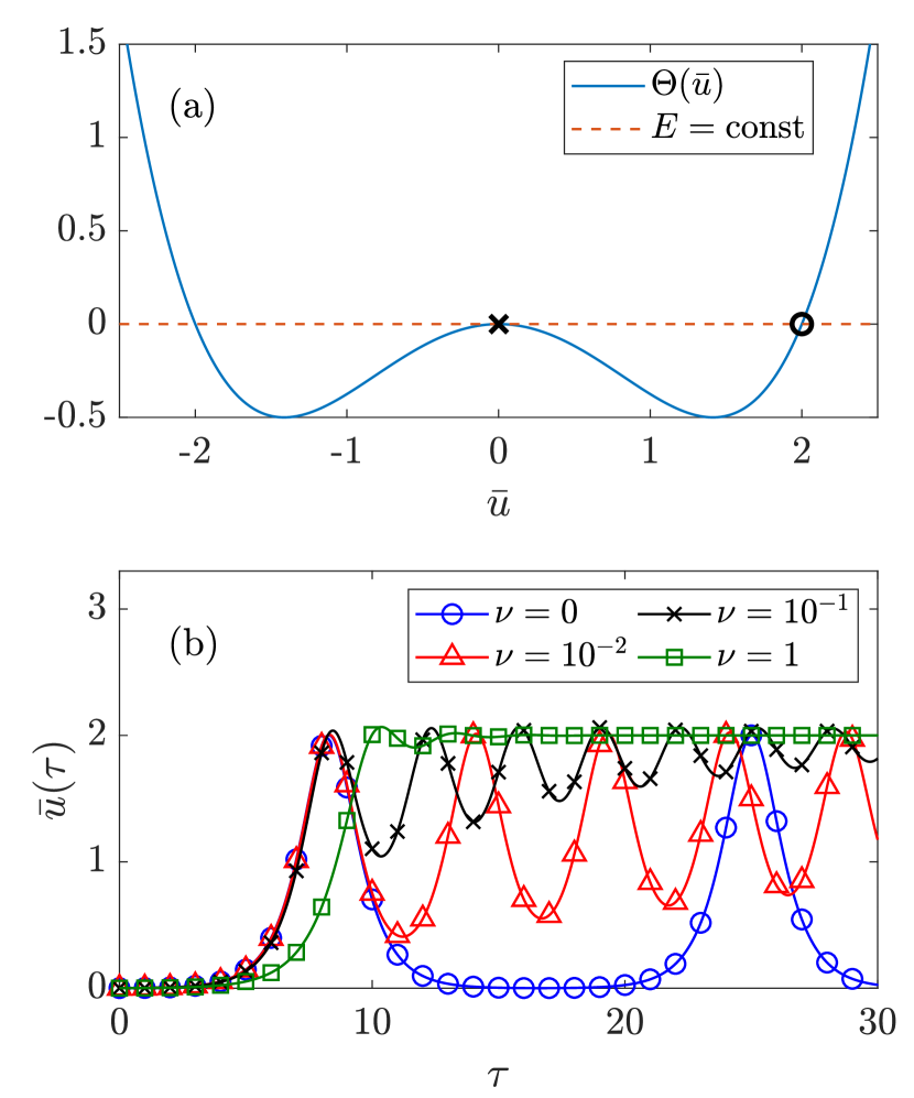
Figure 1: (a) The effective potential $\Theta(\bar{u})$ [Eq. (54)] with $\bar{a}_{0}=4$ (and hence $g^{2}=1>0$). The MI corresponds to a initial condition $\bar{u}=\bar{u}_{0}$ near the origin (black cross, $\bar{u}_{0}=10^{-3}$). At the nonlinear stage, $\bar{u}$ is constrained by the conservation of the “energy”, $E=(d_{\tau}\bar{u})^{2}/2+\Theta$ (dashed line), and hence will start to decrease when reaching $\bar{u}\approx 2$ (black circle). (b) Numerical solutions of the rescaled 4MT system governed by Eqs. (49) and (59). The coefficient $\nu$ in Eq. (59) describes an ad hoc damping that mimics the coupling to other DW sidebands beyond the 4MT. The initial conditions are $\bar{a}=\bar{a}_{0}=4$, $\bar{u}=10^{-3}$, and $\bar{b}=\bar{c}=0$. A transition from oscillations to saturation of $\bar{u}$ is observed as $\nu$ increases.

The 4MT dynamics is numerically illustrated in Fig. 1(b). Unlike the exact solution (56), a finite initial perturbation of $\bar{u}$ results in oscillations with a finite period [Fig. 1(b), blue curve with circles]. We also propose a toy model to illustrate the transition from oscillations to saturation of $\bar{u}$, which adds an ad hoc damping of the sidebands to mimic their coupling to higher harmonics. Specifically, we replace Eq. (49) with

$$\frac{d\bar{b}}{d\tau}=\bar{c}-\nu\bar{b},\quad\frac{d\bar{c}}{d\tau}=-\bar{b}-\left(\bar{a}-\frac{a_{0}}{2}\right)\bar{u}-\nu\bar{c},$$ (59)

where $\nu$ is some positive constant. Then, as we increase $\nu$, a gradual transition from oscillations to saturation of $\bar{u}$ is observed as shown in Fig. 1(b). In particular, at very large $\nu$ such that $\nu\gg d/d\tau$, one has

$$\bar{b}\approx\frac{\bar{c}}{\nu},\quad\bar{c}\approx-\frac{\bar{u}}{\nu}\left(\bar{a}-\frac{\bar{a}_{0}}{2}\right),$$ (60)

and Eq. (49) gives

$$\frac{d\bar{u}}{d\tau}\approx\frac{\bar{a}_{0}\bar{u}}{2\nu}\left(1-\frac{\bar{u}^{2}}{\bar{a}_{0}}\right).$$ (61)

This equation also has an exact solution

$$\bar{u}=\sqrt{\frac{\bar{a}_{0}}{2}}\exp\left(\frac{\bar{a}_{0}}{4\nu}\,\tau\right)\sqrt{{\rm sech}\left(\frac{\bar{a}_{0}}{2\nu}\,\tau\right)},$$ (62)

which describes monotonic saturation of the ZF [Fig. 1(b), green curve with squares]. This shows that, qualitatively, the ZF saturation can be explained as a result of phase mixing that occurs due to the primary-wave coupling to higher harmonics. For quantitative predictions, a more rigorous approach is proposed below based on exploring the drifton phase-space dynamics.

III.2 Control parameter $\boldsymbol{N}$ in the GO limit

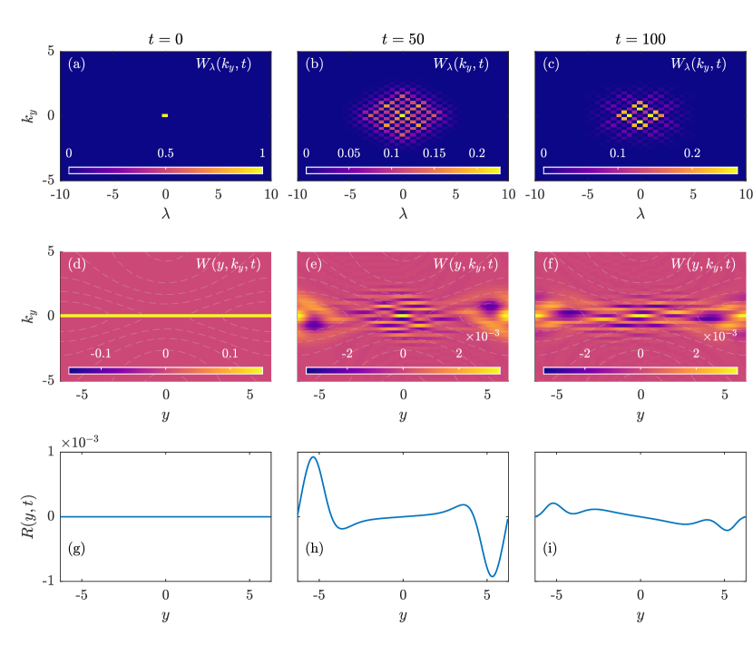
Figure 2: A numerical solution of Eq. (38) on the $(\lambda,k_{y})$ plane with constant $k_{x}=p$ and $257\times 257$ grid points, namely, $-128\leq m,n\leq 128$ [Eq. (43)]. The initial condition is $\bar{W}_{0,0}=1$, and $\bar{W}_{m,n}=0$ for the rest. The ZF amplitude $u$ is kept constant. The parameters are $\alpha=0,$ $\beta=1,$ $L_{{\rm D}}=1,$ $p=2,$ $q=0.5$, and $u=0.05.$ (a)-(e): $|\bar{W}_{m,n}|$ at $t=0$, $50$, and $100$, with $\lambda=mq$ and $k_{y}=nq/2$ at each grid point. (d)-(f): the corresponding Wigner function $W(y,k_{y},t)$ [the inverse Fourier transform of $W_{\lambda}$, Eq. (37)] at the same moments of time, where the gray dashed curves are constant-$\mathcal{H}$ contours [Eq. (36)]. The shape of the distribution function $W(y,k_{y})$ reflects the presence of passing trajectories at $y=0$ and trapped trajectories at $y=\pm\pi/q$. Since the initial condition is delta-shaped in $k_{y}$, the GO assumption is not strictly satisfied, causing $W(y,k_{y},t)$ to be negative in some regions. (g)-(i): the ZF drive $R(y,t)$ [Eq. (65)] at the corresponding moments of time. It is seen that due to the passing trajectories, the slope of $R$ at $y=0$ changes sign. (The associated dataset is available at http://doi.org/10.5281/zenodo.2563449. (zenodo, ))

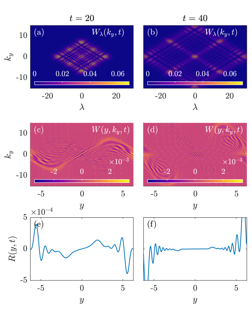
Figure 3: Same as Fig. 2 but for $u=0.4$. First row: $|\bar{W}_{m,n}|$ at $t=20$ and $t=40$. Second row: $W(y,k_{y},t)$ at the corresponding moments of time. The shape of the distribution function $W(y,k_{y})$ reflects the presence of trapped trajectories at $y=\pm\pi/q$ and runaway trajectories at larger-$|k_{y}|$ region. Third row: the ZF drive $R(y,t)$ [Eq. (65)] at the corresponding moments of time. Due to runaways, the slope of $R$ at $y=0$ quickly flattens and stays zero indefinitely. (The associated dataset is available at http://doi.org/10.5281/zenodo.2563449. (zenodo, ))

Let us study the nonlinear stage of the MI using the WKE [Eq. (34)], which naturally accounts for all DW sidebands. As a starting point, we appeal to the findings from Ref. (Zhu18b, ), where three types of drifton phase-space trajectories were identified: trapped, passing, and runaway. (The last one corresponds to driftons leaving to infinity along the $k_{y}$ axis while retaining finite $y$.) It was also found in Ref. (Zhu18b, ) that the drifton phase-space topology for a sinusoidal ZF can vary depending on how the ZF amplitude relates to the following two critical values:

$$u_{c,1}\doteq\frac{\beta}{2p_{{\rm D}}^{2}-(\alpha L_{{\rm D}}^{-2}+q^{2})},\quad u_{c,2}\doteq\frac{\beta}{\alpha L_{{\rm D}}^{-2}+q^{2}}.$$ (63)

The GO limit corresponds to $u_{c,1}\ll u_{c,2}$. At $u<u_{c,1}$ (regime 1), trajectories of all three types are possible; at $u_{c,1}\leq u<u_{c,2}$ (regime 2), passing trajectories vanish; and finally, at $u>u_{c,2}$ (regime 3), trapped trajectories also vanish.

Figures 2 and 3 show the corresponding evolution of $W_{\lambda}$ calculated numerically from Eq. (38) at fixed ZF velocity, namely, $U=u\cos qy$ with constant $u$. Under the GO assumption, the mHME and oHME exhibit similar dynamics, so for clarity, we consider only the mHME ($\alpha=0$). Since $u$ is assumed stationary, Eq. (38) is linear in $W$, and the initial condition is chosen as [Eq. (43)]

$$\bar{W}_{m,n}(t=0)=\delta_{m,0}\delta_{n,0},$$ (64)

where $\delta_{i,j}$ is the Kronecker delta. Figure 2 corresponds to $u<u_{c,1}$ (regime 1). In this case, the distribution $W(y,\boldsymbol{k})$ in the phase space is confined to small $|k_{y}|$ regions enclosed by the contours of passing and trapped trajectories, and no driftons reside on runaway trajectories (transport along $k_{y}$ is suppressed). The corresponding $\bar{W}_{m,n}$ are vanishingly small at large $m$ and $n$; i.e., only a finite number of harmonics are coupled. In contrast, Fig. 3 corresponds to $u_{c,1}<u<u_{c,2}$ (regime 2). In this case, passing trajectories are replaced by runaway trajectories, so driftons can propagate to much larger $|k_{y}|$ (transport along $k_{y}$ is not suppressed). Then, the corresponding $\bar{W}_{m,n}$ has a much wider distribution; i.e., many harmonics are coupled simultaneously.

Now, let us consider the ZF evolution that would be driven by the above dynamics (which we now consider prescribed for simplicity). As seen from Eq. (29), the ZF is driven by the gradient of the (minus) DW momentum flux,

$$R(y,t)\doteq-\langle\tilde{v}_{x}\tilde{v}_{y}\rangle(y,t),$$ (65)

which can be numerically calculated from the Wigner function (Ruiz16, ),

$$R(y,t)=\int\frac{d^{2}kd\lambda}{(2\pi)^{3}}\,\frac{k_{x}k_{y}}{\kappa_{+\lambda}^{2}\kappa_{-\lambda}^{2}}\,W_{\lambda}(\boldsymbol{k},t)e^{i\lambda y}.$$ (66)

The values of $R(y,t)$ are plotted in the lowest rows in Figs 2 and 3. Since $\kappa_{\pm\lambda}^{2}=p_{{\rm D}}^{2}+(k_{y}\pm\lambda/2)^{2}$, runaways with large $|k_{y}|$ contribute little to $R$, so the global dynamics is largely determined by passing driftons. Particularly, consider the slope of $R$ at the ZF peak ($y=0$). In regime 1, this slope oscillates [Figs. 2(g)-(i)], hence causing oscillations of the ZF amplitude. In contrast, in regime 2, this slope quickly flattens and stays zero indefinitely [Figs. 3(g)-(i)]. This is due to the fact that driftons largely accumulate on runaway and trapped trajectories near the ZF troughs ($y=\pm\pi/q$) and thus cannot influence the ZF peak anymore.

Hence, whether a ZF will oscillate or saturate monotonically depends on whether the “control parameter” $N\doteq u_{{\rm max}}/u_{c,1}$ is smaller or larger than unity. One can also make this estimate more quantitative as follows. As discussed above, the DW spectrum is confined to small $|k_{y}|$ when $N\lesssim 1$; hence, the 4MT can be considered as a reasonable model. By using Eq. (58) for $u_{{\rm max}}$, we obtain

$$u_{{\rm max}}\approx\frac{\sqrt{2}\gamma_{{\rm MI}}}{p},\quad u_{c,1}\approx\frac{\beta}{2p_{{\rm D}}^{2}},$$ (67)

where we adopted $\delta,\delta^{\prime}\gg 1$ for the GO limit. Then, $N$ can be expressed as

$$N\approx\frac{2\sqrt{2}\,\gamma_{{\rm MI}}}{\omega_{{\rm DW}}},\quad\omega_{{\rm DW}}\doteq\frac{\beta p}{p_{{\rm D}}^{2}},$$ (68)

where $\omega_{{\rm DW}}$ can be recognized as the (absolute value of) the characteristic DW frequency. In summary, the ZF oscillates if $\gamma_{{\rm MI}}\ll\omega_{{\rm DW}}$ and monotonically saturates otherwise.

III.3 Modifications due to full-wave effects

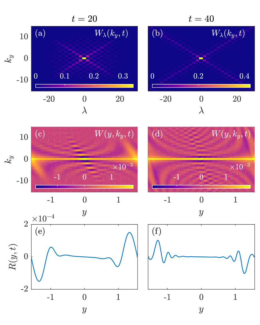
Figure 4: Same as Fig. 2 but for $q=2$ and $u=0.2$. Due to the large ZF wavenumber $q$, full-wave effects are significant. Namely, $|\bar{W}_{m,n}|$ are localized along the diagonals $k_{y}=\pm\lambda/2$. Also, $W(y,k_{y},t)$ cannot be easily interpreted as the drifton distribution function. Instead, each drifton is smeared out in the phase space. (The associated dataset is available at http://doi.org/10.5281/zenodo.2563449. (zenodo, ))

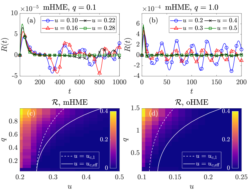
Figure 5: (a) and (b): Numerical solutions of Eq. (38) at fixed ZF amplitude $u$ for $\alpha=0$ (mHME) and $\beta=L_{{\rm D}}=p=1$. (a) The ZF drive $R(t)$ [Eq. (71)] at $y=0$ for various values of $u$ versus $t$ at $q=0.1$, which corresponds to $u_{c,1}\approx 0.25$ [Eq. (63)]. $R(t)$ oscillates when $u<u_{c,1}$ and decays to zero when $u>u_{c,1}$. (b) Same as (a) but for $q=1.0$, which corresponds to $u_{c,1}\approx 0.33$. The critical amplitude, when $R(t)$ decays to zero, becomes larger than $u_{c,1}$ and is estimated from Eq. (73). (c) and (d): A parameter scan over $q$ and $u$ for determining the critical ZF amplitude above which $R(t)$ decays to zero. The parameters are $\beta=L_{{\rm D}}=1$, $\alpha=0$ (mHME) and $p=1$ in (c), and $\alpha=1$ (oHME) and $p=2$ in (d). Shown in color is the value of $\mathcal{R}$ [Eq. (72)]. The white dashed and solid curves are $u=u_{c,1}$ and $u=u_{c,{\rm eff}}$. The latter roughly matches the threshold beyond which $\mathcal{R}$ is negligible. (The associated dataset is available at http://doi.org/10.5281/zenodo.2563449. (zenodo, ))

At large enough $q$, the WKE (34) ceases to be valid and one must take into account the deviations from the GO approximation. These deviations are called full-wave effects and can be understood from the coupling between harmonics in Eq. (37). At large $q$, the coupling coefficient $Q$ deviates from unity and becomes inhomogeneous [Eq. (39)]. Recall that

$$\kappa_{a}^{2}\doteq p_{{\rm D}}^{2}+\left(k_{y}+\frac{a}{2}\right)^{2},$$ (69)

hence the minimum value of $Q_{a}$ is achieved at $k_{y}+a/2=0$, and

$$\min Q=1-\delta_{\alpha}^{-1},\quad\delta_{\alpha}\doteq\frac{p_{{\rm D}}^{2}}{\alpha L_{{\rm D}}^{-2}+q^{2}}.$$ (70)

(Note that $\delta_{\alpha}>1$ is a necessary condition for the MI to happen, and hence $\min Q>0$.) When $\min Q\ll 1$, it can be seen from Eq. (39) that the modes along the diagonals $k_{y}=\pm\lambda/2$ are decoupled from the rest and the initial perturbation $\bar{W}_{0,0}$ propagates mainly along the diagonals, as demonstrated in Fig. 4.

When full-wave effects are important, the critical ZF amplitude can deviate from $u_{c,1}$ given by Eq. (63). Here, we study the critical ZF amplitude by numerically integrating Eq. (38) with stationary $u$ and recording the ZF drive at $y=0$, namely,

$$R(t)\doteq\partial_{y}R(y,t)|_{y=0}=-\partial_{y}\langle\tilde{v}_{x}\tilde{v}_{y}\rangle(y,t)|_{y=0}.$$ (71)

Specifically, we calculate

$$\mathcal{R}\doteq\sqrt{\frac{\overline{R^{2}(t)}}{\max R^{2}(t)}},$$ (72)

where $\overline{\cdot\cdot\cdot}$ is the time-average. (To exclude the initial transient dynamics, only the interval $0.25T<t<T$ is used for the time-averaging, where $T$ is the total integration time.) The critical amplitude is defined as the value of $u$ beyond which $\mathcal{R}$ becomes negligible.

As shown in Figs. 5(c) and (d), the critical amplitude starts to deviate from $u_{c,1}$ as $q$ increases. The following empirical correction can be adopted to account for the finite $q$-dependence of the critical amplitude:

$$u_{c,1}\to u_{c,{\rm eff}}\doteq\frac{u_{c,1}}{1-0.5\delta_{\alpha}^{-1}},$$ (73)

as seen in Figs. 5(c) and (d). Then, the control parameter (68) becomes

$$N =\frac{2\sqrt{2}\gamma_{{\rm MI}}}{\omega_{{\rm DW}}}\,\sqrt{\frac{\delta(\delta+1)}{\delta^{\prime}(\delta^{\prime}-1)}}\,\left(1-\frac{1}{2\delta_{\alpha}}\right)^{2},$$ (74)

where $\delta,$ $\delta^{\prime}$, and $\delta_{\alpha}$ are given by Eqs. (26) and (70). The ZF oscillates at $N\ll 1$ and saturates at $N\gtrsim 1$.

IV Numerical simulations

IV.1 Parameter scan

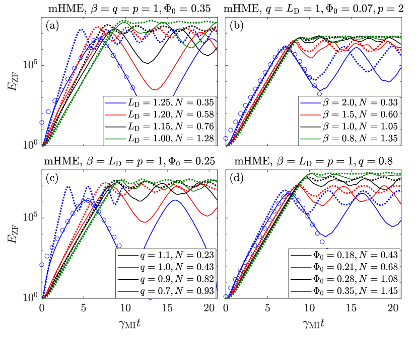
Figure 6: Numerical simulations of the QL (solid lines) and the NL mHWE (dotted lines, using the same parameters). The blue circles are the corresponding 4MT solutions (56). Shown is the ZF energy $E_{{\rm ZF}}$ [Eq. (77)] in units $E_{{\rm ZF}}(t=0)$ versus time $t$ in units $\gamma_{{\rm MI}}^{-1}$ [Eq. (25)]. The specific parameters are presented in the corresponding figures. The initial conditions are given by Eq. (76). The best agreement between the QL and NL simulations can be found in the $\beta$-scan [figure (b)], when the GO approximation is satisfied with the highest accuracy ($\delta_{\alpha}=5$). (The associated dataset is available at http://doi.org/10.5281/zenodo.2563449. (zenodo, ))

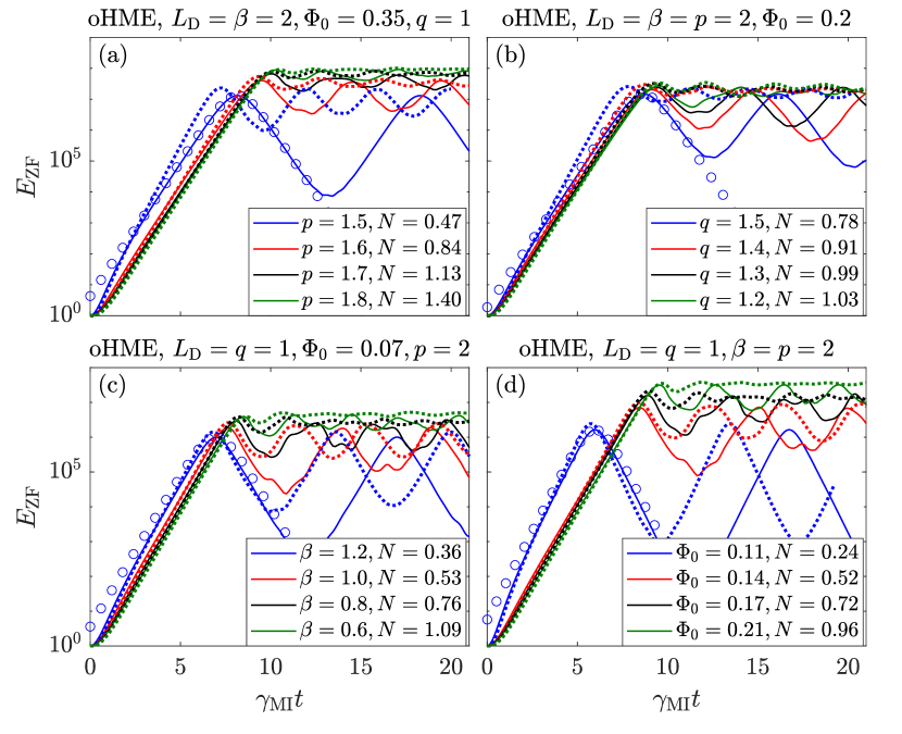
Figure 7: Same as in Fig. 6, but for the oHME ($\alpha=1$). Good agreement between the QL and NL simulations can be found in the $\beta$-scan and $\Phi_{0}$-scan [figures (c) and (d)], when the GO approximation is well satisfied ($\delta_{\alpha}=2.5$). (The associated dataset is available at http://doi.org/10.5281/zenodo.2563449. (zenodo, ))

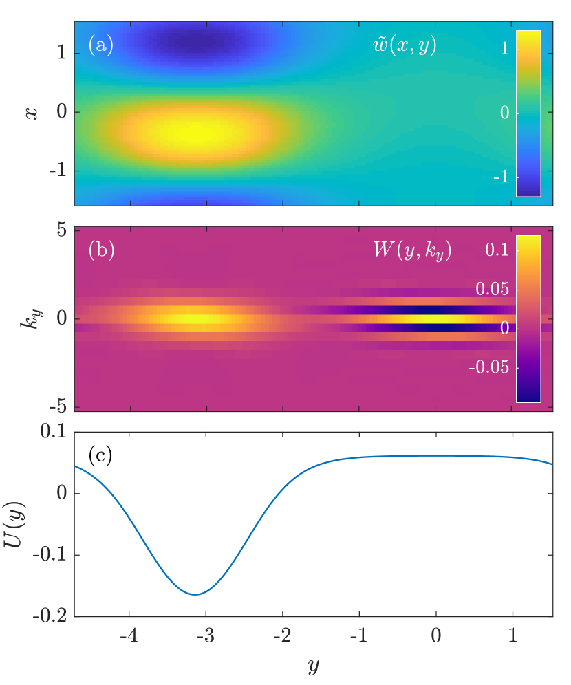
Figure 8: A snapshot of the DW vorticity field $\tilde{w}(x,y)$, the corresponding Wigner function $W(y,k_{y})$, and the ZF profile $U(y)$, at $\gamma_{{\rm MI}}t=7$ of the $\beta=2.0$ case in Fig. 6(b) (QL mHME simulations). At $U<0$, the vortex structure in $\tilde{w}$ corresponds to the trapped drifton distribution in $W$; at $U>0$, the absence of $\tilde{w}$ corresponds to driftons following passing trajectories and leaving this region. The striped structure in figure (b) is due to the interference between the shown trapped distribution and a similar distribution on the next spatial period (not shown). Such structures are discussed in further detail in Ref. (soliton, ). (The associated dataset is available at http://doi.org/10.5281/zenodo.2563449. (zenodo, ))

In order to test the above theory of the ZF fate beyond the linear stage, we numerically integrated both the the QL system [Eqs. (28) and (29)] and the NL system [Eqs. (1) and (2)] for various parameters such that

$$0<N\lesssim 1,\quad\delta_{\alpha}\gtrsim 1.$$ (75)

The second requirement means $\delta_{\alpha}$ shall not be too large, i.e., $q^{2}$ shall not be too small, because then ZF harmonics with wave numbers that are multiples of $q$ have higher growth rates and outpace the fundamental harmonic at the linear stage (see more discussions in Sec. V.1). Overall there are five parameters that determine the system dynamics at the nonlinear stage: $L_{{\rm D}}$, $p$, $\beta$, $q$, and $\Phi_{0}$. For the mHME ($\alpha=0$), we vary only $L_{{\rm D}}$, $\beta$, $q$, and $\Phi_{0}$, because $L_{{\rm D}}$ and $p$ mainly appear as a combination $L_{{\rm D}}^{-2}+p^{2}$, and the remaining $p$ in Eq. (38) only defines the time scale and can be absorbed by a variable transformation $t\to pt$. For the oHME ($\alpha=1$), we vary only $p$, $\beta$, $q$, and $\Phi_{0}$, because it is hard to satisfy the requirement (75) when $L_{{\rm D}}$ is varied with other parameters fixed. For both the oHME and the mHME, the initial conditions are chosen to be

$$\tilde{\varphi}=2\Phi_{0}\cos px,\quad U=u\cos qy,\quad u\ll p\Phi_{0},$$ (76)

where $\Phi_{0}$ is real

The simulation results of the QL and NL systems are shown in Figs. 6 (mHME) and 7 (oHME), where we plot the ZF energy

$$E_{{\rm ZF}}(t)\doteq\frac{1}{2}\int dy[U(y,t)]^{2}$$ (77)

versus time $t$. As predicted by our theory, in QL simulations, ZFs oscillate at the nonlinear stage if $N\ll 1$ and largely saturate monotonically if $N\gtrsim 1$. For comparison, we also plot the corresponding 4MT solutions (56) for the smallest-$N$ cases in each figure. The fact that the 4MT solutions agree with predictions of the QL theory confirms the 4MT applicability at the nonlinear stage of the MI in the weak-ZF limit.

Note that the ZF energy has a larger maximum at larger $N$. This is explained as follows. At larger $N$, driftons propagate to larger wave numbers and hence end up with lower energy, which is given by (Ruiz16, )

$$E_{{\rm DW}}(t)\doteq\frac{1}{2}\int\frac{d^{2}kdy}{(2\pi)^{2}}\,\frac{W(y,\boldsymbol{k},t)}{k_{{\rm D}}^{2}}.$$ (78)

Due to the total energy conservation, this leaves more energy for the ZFs.

In Figs. 6 and 7, NL simulation results are also shown for the same parameters. The transition from ZF oscillations to saturation is also recovered from these simulations. However, in terms of the oscillation amplitudes and frequencies, good agreement between QL and NL simulations occurs only when the GO approximation is satisfied with reasonable accuracy, say, at

$$\delta_{\alpha}\gtrsim 3.$$ (79)

At smaller $\delta_{\alpha}$, NL simulations show much smaller amplitudes of the ZF oscillations due to the additional DW–DW self-interactions. A brief explanation of the discrepancy between QL and NL simulations is given in Sec. IV.2.

In Fig. 8, we show a snapshot of the DW vorticity $\tilde{w}(x,y)$, the corresponding Wigner function $W(y,k_{y})$, and the ZF profile $U(y)$ from a QL mHME simulation. The snapshot is taken at $\gamma_{{\rm MI}}t=7$ of the $\beta=2.0$ case in Fig. 6(b). This corresponds to the time when the ZF energy reaches the maximum and is about to reverse. The DW vortex structure at $U<0$ is clearly seen and corresponds to trapped driftons in the phase space. In contrast, there is almost no DW activity at $U>0$, because driftons follow passing trajectories and have left this region. At this stage, the ZF velocity is no longer sinusoidal, and have a deep trough and a flat peak. This shape of the ZF is due to the larger ZF drive [Eq. (66)] induced by the trapped trajectories at the ZF trough, and hence cause the ZF to have a larger local amplitude. After this moment of time, passing driftons return to the ZF top since the system is periodic in $y$, and reduce the ZF amplitude; correspondingly, the ZF energy oscillates, as in Fig. 6(b).

IV.2 Difference between the QL and NL models

Here, we discuss why good agreement between QL and NL systems can be achieved when the GO approximation is well satisfied, and why discrepancies arise otherwise. Recall that the MI growth rate $\gamma_{{\rm MI}}$ (25) derived from the 4MT is exact for the QL model but not for the corresponding NL model. Therefore, it is expected that the discrepancy can be attributed, at least partly, to the difference between the QL and NL growth rates. We compare these growth rates by comparing the relative amplitude between the second DW sideband and the first DW sideband at the linear stage, the former being excluded from the 4MT. From Eq. (3), we have

$$\epsilon_{{\rm NL}}\doteq\left|\frac{\partial_{t}\varphi_{2\boldsymbol{p}+\boldsymbol{q}}}{\partial_{t}\varphi_{\boldsymbol{p}+\boldsymbol{q}}}\right|\sim\left|\frac{T(2\boldsymbol{p}+\boldsymbol{q},\boldsymbol{p}+\boldsymbol{q},\boldsymbol{p})\Phi_{0}\varphi_{\boldsymbol{p}+\boldsymbol{q}}}{T(\boldsymbol{p}+\boldsymbol{q},\boldsymbol{q},\boldsymbol{p})\Phi_{0}\varphi_{\boldsymbol{q}}}\right|$$ (80)

as a measure of the importance of NL effects. Also, $|\varphi_{\boldsymbol{p}}|=|\Phi_{0}|$ is assumed at the linear stage. From Eq. (5), the coupling coefficients are

$$|T(2\boldsymbol{p}+\boldsymbol{q},\boldsymbol{p}+\boldsymbol{q},\boldsymbol{p})|=\frac{q^{2}}{L_{{\rm D}}^{-2}+4p^{2}+q^{2}}\,pq,$$

$$|T(\boldsymbol{p}+\boldsymbol{q},\boldsymbol{q},\boldsymbol{p})|=\frac{(1-\alpha)L_{{\rm D}}^{-2}+p^{2}-q^{2}}{L_{{\rm D}}^{-2}+p^{2}+q^{2}}\,pq.$$

Then

$$\epsilon_{{\rm NL}}\sim\left|\frac{\varphi_{\boldsymbol{p}+\boldsymbol{q}}}{\varphi_{\boldsymbol{q}}}\right|\frac{q^{2}}{L_{{\rm D}}^{-2}+4p^{2}+q^{2}}\,\frac{L_{{\rm D}}^{-2}+p^{2}+q^{2}}{(1-\alpha)L_{{\rm D}}^{-2}+p^{2}-q^{2}}.$$ (81)

In the above expression for $\epsilon_{{\rm NL}}$, the first term $|\varphi_{\boldsymbol{p}+\boldsymbol{q}}/\varphi_{\boldsymbol{q}}|$ can be estimated from the 4MT equation (8), which gives

$$\left|\frac{\partial_{t}\varphi_{\boldsymbol{p}+\boldsymbol{q}}}{\partial_{t}\varphi_{\boldsymbol{q}}}\right|\sim\left|\frac{T(\boldsymbol{p}+\boldsymbol{q},\boldsymbol{q},\boldsymbol{p})\Phi_{0}\varphi_{\boldsymbol{q}}}{T(\boldsymbol{q},-\boldsymbol{p},\boldsymbol{p}+\boldsymbol{q})\Phi_{0}\varphi_{\boldsymbol{p}+\boldsymbol{q}}}\right|.$$ (82)

Since $\partial_{t}\varphi_{\boldsymbol{p}+\boldsymbol{q}}/\partial_{t}\varphi_{\boldsymbol{q}}\sim\varphi_{\boldsymbol{p}+\boldsymbol{q}}/\varphi_{\boldsymbol{q}}$ and $|T(\boldsymbol{q},-\boldsymbol{p},\boldsymbol{p}+\boldsymbol{q})|=pq$, this gives

$$\left|\frac{\varphi_{\boldsymbol{p}+\boldsymbol{q}}}{\varphi_{\boldsymbol{q}}}\right|\sim\sqrt{\frac{(1-\alpha)L_{{\rm D}}^{-2}+p^{2}-q^{2}}{L_{{\rm D}}^{-2}+p^{2}+q^{2}}},$$ (83)

and thus

$$\epsilon_{{\rm NL}}\sim\frac{q^{2}}{L_{{\rm D}}^{-2}+4p^{2}+q^{2}}\left(\frac{\delta+1}{\delta_{\alpha}-1}\right)^{1/2},$$ (84)

where $\delta$ and $\delta_{\alpha}$ are given by Eqs. (26) and (70), respectively. When $\delta,\delta_{\alpha}\gg 1$, i.e., $q^{2}\ll p^{2}+(1-\alpha)L_{{\rm D}}^{-2}$, one obtains $\epsilon_{{\rm NL}}\ll 1$. Then, NL effect is expected to be small, and hence QL and NL simulations produce similar results. In contrast, when $\delta_{\alpha}$ approaches unity, $\epsilon_{{\rm NL}}$ can become of order one. Then, the QL model ceases to be an adequate approximation to the NL model.

The above estimate also indicates that, at least for the mHME, when $p^{2}\gtrsim L_{{\rm D}}^{-2}$, one has

$$\epsilon_{{\rm NL}}\sim\frac{\epsilon_{{\rm GO}}}{4}\sqrt{\frac{1+\epsilon_{{\rm GO}}}{1-\epsilon_{{\rm GO}}}},$$ (85)

where $\epsilon_{{\rm GO}}\sim\delta^{-1}\ll 1$ under the GO approximation. Therefore, $\epsilon_{{\rm NL}}\ll 1$ at $\epsilon_{{\rm GO}}\ll 1$ and $\epsilon_{{\rm NL}}\gtrsim 1$ when $\epsilon_{{\rm GO}}$ approaches unity (and the MI vanishes when $\epsilon_{{\rm GO}}>1$). Hence, the applicability domain of the QL approximation is roughly the same as that of the GO approximation.

V Comparison with previous studies

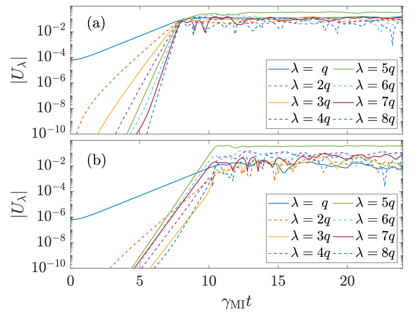
Figure 9: Numerical simulations of the QL oHME, which corresponds to the $M=1$ case in Ref. (Connaughton10, ). The parameters are $L_{{\rm D}}^{-2}=0,$ $\beta=p=10$, $q=1$, and $\Phi_{0}=10^{-2}$. The initial ZF perturbation is $U(y,t=0)=u\cos qy$. Shown are the amplitudes of the ZF harmonics $|U_{\lambda}|$ for different $\lambda$: (a) $u=2\times 10^{-5}$ and (b) $u=2\times 10^{-7}$. The time $t$ is normalized to $\gamma_{{\rm MI}}^{-1}$ of the fundamental harmonic $\lambda=q$. Since higher harmonics have larger MI growth rates, they grow faster and eventually, in (b), outpace the fundamental harmonic. For the larger initial ZF perturbation in (a), which is also assumed in Ref. (Connaughton10, ), higher harmonics are not as strong as in (b) because the linear stage ends sooner. Nevertheless, higher harmonics around $\lambda=5q$ still dominate at the nonlinear stage. Therefore, one should replace $q$ by $5q$ in the calculation of $N$ in order to achieve the correct prediction. (The associated dataset is available at http://doi.org/10.5281/zenodo.2563449. (zenodo, ))

V.1 Control parameters: $\boldsymbol{N}$ versus $\boldsymbol{M}$

Let us also compare our results with those in Refs. (Connaughton10, ; Gallagher12, ) where related simulations were performed. Specifically, Ref. (Connaughton10, ) reports NL oHME simulations for $p^{2}\gg q^{2}$ and $L_{{\rm D}}^{-2}=0$. Also, Ref. (Gallagher12, ) reports NL mHME simulations; however, the parameter is chosen such that $p^{2}\gg q^{2},L_{{\rm D}}^{-2}$, and the resulting dynamics is almost identical to that in the oHME. In both cases, the GO assumption is well satisfied ($\delta,\delta^{\prime},\delta_{\alpha}\approx 100\gg 1$). Hence, the difference between NL and QL simulations is expected to be small (see Sec. IV.2), and the results of Refs. (Connaughton10, ; Gallagher12, ) can be compared with ours within the scope of the QL approximation. (We have indeed been able to reproduce all the related results from QL simulations using the same parameters as in Refs. (Connaughton10, ; Gallagher12, ), but we choose not to duplicate the figures here.) Due to the similar choice of the parameters in Ref. (Connaughton10, ) and Ref. (Gallagher12, ), we compare with Ref. (Connaughton10, ) only.

Within the GO limit, our control parameter $N$ [Eq. (74)] is

$$N\approx\frac{2\sqrt{2}\,p\gamma_{{\rm MI}}}{\beta},\quad\gamma_{{\rm MI}}\approx\sqrt{2p^{2}q^{2}|\Phi_{0}|^{2}-\left(\frac{\beta q^{2}}{p^{3}}\right)^{2}}.$$ (86)

A different parameter was proposed in Ref. (Connaughton10, ), namely,

$$M\doteq\frac{p^{3}\Phi_{0}}{\beta}.$$ (87)

The authors argue that $M\ll 1/3$ corresponds to ZF oscillations and $M\gtrsim 1/3$ corresponds to monotonic ZF saturation. However, in contrast to our quantitative derivations, only a qualitative argument is provided in Ref. (Connaughton10, ) (also see Sec. V.2). As a result, the parameter $M$ cannot describe the sensitive dependence on $q$ or $L_{{\rm D}}$, as our $N$ does in Figs. 6(a), 6(c), and 7(b). Our $N$ is also better in terms of the predictive power. For example, for the case of $\beta=1.2$ in Fig. 7(c), one has $M=0.47>1/3$, so the ZF is supposed to saturate; however, the ZF actually oscillates, which can be predicted by our $N=0.36<1$.

We note that our theory can also predict the outcomes of three numerical examples used in Ref. (Connaughton10, ), where $M=0.1$, $1$, and $10$, respectively. For $M=0.1$ and $M=10$, our control parameter takes the values $N=0.028$ and $N=3.94$, respectively; hence, our theory predicts that the ZF oscillates in the former case and saturates monotonically in the latter case, which is indeed observed in Ref. (Connaughton10, ). However, Ref. (Connaughton10, ) reports ZF saturation at $M=1$, while our $N=0.39<1$. It may seem then that our theory predicts ZF oscillations instead of saturation, which would be incorrect. Actually, due to the small $q$ in this case, high harmonics of the ZF have much larger linear growth rates and outpace the fundamental harmonic (Fig. 9). This makes our analytic model inapplicable, for it assumes a quasi-sinusoidal ZF. That said, if one calculates $N$ by replacing $q$ with the wave number of the dominant harmonic, then $N$ becomes larger than unity and the ZF saturation is readily anticipated.

V.2 Relevance of the Rayleigh–Kuo threshold for the ZF saturation

The authors of Ref. (Connaughton10, ) proposed a brief explanation of the physical meaning of their parameter $M$, which is as follows. First, they assumed that DWs transfer an order-one fraction of their energy to ZFs, so the ZF maximum amplitude is

$$u_{{\rm max}}\sim p\Phi_{0}.$$ (88)

Second, they speculated that the ZF saturates when it reaches the Rayleigh–Kuo (RK) threshold (Kuo49, )

$$\partial_{y}^{2}U(y)-\beta>0.$$ (89)

We believe that this explanation is problematic, namely, for two reasons. First, the estimate (88) contradicts the 4MT estimate (58) that we have confirmed numerically (Figs. 6 and 7). A more accurate estimate within the GO regime would be $u_{{\rm max}}\gtrsim 2q\Phi_{0}$. (Note that this estimate reinstates the dependence on $q$, which is absent in $M$.) Second, the RK criterion does not describe the ZF saturation but rather determines the threshold of the instability of the Kelvin–Helmholtz type that destroys the ZF. (It is also called the “tertiary instability” by some authors (Rogers00, ; Zhu18a, ; Zhu18b, ; Kuo49, ; Zhu18c, ; Numata07, ; Kim2002, ; Rath18, ), and in previous studies we showed that this instability does not exist in the GO limit (Zhu18a, ; Zhu18b, ; Zhu18c, ).) Since the RK threshold corresponds to $u>u_{c,2}$ (Sec. III.2), and $u_{c,2}\gg u_{c,1}$ in the GO regime, we claim that ZFs saturate before the RK threshold is reached. In summary, we believe that our parameter $N$ is more substantiated than the parameter $M$ introduced in Refs. (Connaughton10, ; Gallagher12, ). We also emphasize that our theory withstands the test of numerical simulations, as shown in Sec. IV.1.

VI Conclusions

In this paper we propose a semi-analytic theory that explains the transition between the oscillations and saturation of collisionless ZFs within the QL HME. By analyzing phase-space trajectories of driftons within the GO approximation, we argue that the parameter that controls this transition is $N\sim\gamma_{{\rm MI}}/\omega_{{\rm DW}}$, where $\gamma_{{\rm MI}}$ is the MI growth rate and $\omega_{{\rm DW}}$ is the linear DW frequency. We argue that at $N\ll 1$, ZFs oscillate due to the presence of so-called passing drifton trajectories, and we derive an approximate formula for the ZF amplitude as a function of time in this regime. In doing so, we also extend the applicability of the popular 4MT model, which is commonly used for the linear stage, to nonlinear ZF–DW interactions. We also show that at $N\gtrsim 1$, the passing trajectories vanish and ZFs saturate monotonically, which can be attributed to phase mixing of higher-order sidebands. A modification of $N$ that accounts for effects beyond the GO limit is also proposed. These analytic results are tested against both QL and NL simulations. They also explain the earlier numerical results by Refs. (Connaughton10, ; Gallagher12, ) and offer a revised perspective on what the control parameter is that determines the transition from oscillations to saturation of collisionless ZFs.

- (1) Z. Lin, T. S. Hahm, W. W. Lee, W. M. Tang, and R. B. White, Science 281, 1835 (1998).
- (2) P. H. Diamond, S.-I. Itoh, K. Itoh, and T. S. Hahm, Plasma Phys. Controlled Fusion 47, R35 (2005).
- (3) B. N. Rogers, W. Dorland, and M. Kotschenreuther, Phys. Rev. Lett. 85, 5336 (2000).
- (4) F. Jenko, W. Dorland, M. Kotschenreuther, and B. N. Rogers, Phys. Plasmas 7, 1904 (2000).
- (5) A. R. Vasavada and A. P. Showman, Rep. Prog. Phys 68, 1935 (2005).
- (6) A. I. Smolyakov, P. H. Diamond, and V. I. Shevchenko, Phys. Plasmas 7, 1349 (2000).
- (7) A. I. Smolyakov, P. H. Diamond, and M. Malkov, Phys. Rev. Lett. 84, 491 (2000).
- (8) D. Strintzi and F. Jenko, Phys. Plasmas 14, 042305 (2007);
- (9) K. Srinivasan and W. R. Young, J. Atmos. Sci. 69, 1633 (2012).
- (10) J. B. Parker and J. A. Krommes, Phys. Plasmas 20, 100703 (2013).
- (11) J. B. Parker and J. A. Krommes, New J. Phys. 16, 035006 (2014).
- (12) J. B. Parker, Ph.D. thesis, Princeton University (2014).
- (13) D. A. St-Onge and J. A. Krommes, Phys. Plasmas 24, 042107 (2017).
- (14) J. B. Marston, G. P. Chini, and S. M. Tobias, Phys. Rev. Lett. 116, 214501 (2016).
- (15) D. Qi and A. J. Majda, arXiv:1901.08590.
- (16) L. Chen, Z. Lin, and R. White, Phys. Plasmas 7, 3129 (2000).
- (17) C. P. Connaughton, B. T. Nadiga, S. V. Nazarenko, and B. E. Quinn, J. Fluid Mech. 654, 207 (2010).
- (18) S. Gallagher, B. Hnat, C. Connaughton, S. Nazarenko, and G. Rowlands, Phys. Plasmas 19, 122115 (2012).
- (19) C. Connaughton, S. Nazarenko, and B. Quinn, Phys. Rep. 604, 1 (2015).
- (20) S. Champeaux and P. H. Diamond, Phys. Lett. A 288, 214 (2001).
- (21) O. Koshkarov, A. I. Smolyakov, and J. T. Mendonça, Plasma Phys. Rep. 42, 769 (2016).
- (22) V. M. Lashkin, Phys. Plasmas 15, 124502 (2008).
- (23) F. Jenko, Phys. Lett. A 351, 417 (2006).
- (24) P. K. Shukla and L. Stenflo, Eur. Phys. J. D 20, 103 (2002).
- (25) G. Manfredi, C. M. Roach, and R. O. Dendy, Plasma Phys. Control. Fusion 43, 825 (2001).
- (26) C. N. Lashmore-Davies, D. R. McCarthy, and A. Thyagaraja, Phys. Plasmas 8, 5121 (2001).
- (27) A. C. Mahanti, Arch. Met. Geoph. Biokl., Ser. A, 30, 211 (1981).
- (28) A. E. Gill, Geophys. Astrophys. Fluid Dyn. 6, 29 (1974).
- (29) D. A. St-Onge, J. Plasma Phys. 83, 905830504 (2017).
- (30) N. C. Constantinou and J. B. Parker, Astrophys. J. 863, 46 (2018).
- (31) B. F. Farrell and P. J. Ioannou, J. Atmospheric Sci. 64, 3652 (2007).
- (32) N. A. Bakas, N. C. Constantinou, and P. J. Ioannou J. Atmospheric Sci. 72, 1689 (2015).
- (33) D. E. Ruiz, J. B. Parker, E. L. Shi and I. Y. Dodin, Phys. Plasmas 23, 122304 (2016).
- (34) D. E. Ruiz, M. E. Glinsky, and I. Y. Dodin, J. Plasma Phys. 85, 905850101 (2019).
- (35) H. Zhu, Y. Zhou, D. E. Ruiz, and I. Y. Dodin, Phys. Rev. E 97, 053210 (2018).
- (36) H. Zhu, Y. Zhou, and I. Y. Dodin, Phys. Plasmas 25, 072121 (2018).
- (37) J. B. Parker, J. Plasma Phys. 82, 595820602 (2016).
- (38) A. I. Smolyakov and P. H. Diamond, Phys. Plasmas 6, 4410 (1999).
- (39) P. Kaw, R. Singh, and P. H. Diamond, Plasma Phys. Controlled Fusion 44, 51 (2002).
- (40) M. A. Malkov, P. H. Diamond, and A. Smolyakov, Phys. Plasmas 8, 1553 (2001).
- (41) K. Miki, P. H. Diamond, Ö. D. Gürcan, G. R. Tynan, T. Estrada, L. Schmitz, and G. S. Xu, Phys. Plasmas 19, 092306 (2012).
- (42) P. H. Diamond and Y.-M. Liang, Phys. Rev. Lett. 72, 2565 (1994).
- (43) E.-J. Kim and P. H. Diamond, Phys. Rev. Lett. 90, 185006 (2003).
- (44) V. Berionni and Ö. D. Gürcan, Phys. Plasmas 18, 112301 (2011).
- (45) S. Kobayashi, Ö. D. Gürcan, and P. H. Diamond, Phys. Plasmas 22, 090702 (2015).
- (46) A. Hasegawa and K. Mima, Phys. Rev. Lett. 39, 205 (1977).
- (47) F. V. Dolzhansky, Fundamentals of Geophysical Hydrodynamics (Springer-Verlag Berlin Heidelberg, 2013), Chap. 7.
- (48) J. A. Krommes and C.-B. Kim, Phys. Rev. E 62, 8508 (2000).
- (49) G. W. Hammett, M. A. Beer, W. Dorland, S. C. Cowley, and S. A. Smith, Plasma Phys. Control. Fusion 35, 973 (1993).
- (50) Y. Zhou, H. Zhu, and I. Y. Dodin, Formation of solitary zonal structures via the modulational instability, in preparation.
- (51) N. D. Cartwright, Physica A 83, 210 (1976).
- (52) H. Zhu, Y. Zhou, and I. Y. Dodin (2019). Nonlinear saturation and oscillations of collisionless zonal flows, Zenodo. http://doi.org/10.5281/zenodo.2563449.
- (53) H. L. Kuo, J. Meteorol. 6, 105 (1949).
- (54) H. Zhu, Y. Zhou, and I. Y. Dodin, Phys. Plasmas 25, 082121 (2018).
- (55) R. Numata, R. Ball, and R. L. Dewar, Phys. Plasmas 14, 102312 (2007).
- (56) E.-J. Kim and P. H. Diamond, Phys. Plasmas 9, 4530 (2002).
- (57) F. Rath, A. G. Peeters, R. Buchholz, S. R. Grosshauser, F. Seiferling, and A. Weikl, Phys. Plasmas 25, 052102 (2018).