Squeezed tensor non-Gaussianity in non-attractor inflation

Ogan Özsoy^⋆, Maria Mylova^⋆, Susha Parameswaran^†, Cari Powell^⋆,

Gianmassimo Tasinato^⋆, Ivonne Zavala^⋆

^⋆ Physics Department, Swansea University, Swansea, SA2 8PP, UK
^† Department of Mathematical Sciences, University of Liverpool, Liverpool, L69 7ZL, UK

  We investigate primordial tensor non-Gaussianity in single field inflation, during a phase of non-attractor evolution when the spectrum of primordial tensor modes can be enhanced to a level detectable at interferometer scales. Making use of a tensor duality we introduced in [1], we analytically compute the full bispectrum of primordial tensor fluctuations during the non-attractor era. During this epoch the shape of the tensor bispectrum is enhanced in the squeezed limit, its amplitude can be amplified with respect to slow-roll models, and tensor non-Gaussianity can exhibit a scale dependence distinctive of our set-up. We prove that our results do not depend on the frame used for the calculations. Squeezed tensor non-Gaussianity induces a characteristic quadrupolar anisotropy on the power spectrum of the stochastic background of primordial tensor perturbations. As a step to make contact with gravitational wave experiments, we discuss the response function of a ground based Michelson interferometer to a gravitational wave background with such a feature.  

1 Introduction

The possibility to directly detect a stochastic background of primordial tensor modes with gravitational wave experiments would offer new ways to probe the physics of inflation. Such an opportunity would allow us to probe a much larger range of frequency scales than what can be tested with CMB physics. Various scenarios have been proposed for enhancing the primordial tensor spectrum at interferometer scales: from coupling the inflation to additional fields, whose dynamics are characterised by instabilities that amplify the tensor spectrum (see e.g. [2, 3, 4, 5, 6, 7, 8, 9, 10, 11, 12, 13, 14, 15, 16, 17, 18, 19, 20, 21, 22, 23, 24]), to models that break space-time symmetries during inflation, leading to a blue spectrum for primordial tensor modes (see e.g. [25, 26, 27, 28, 29, 30, 31, 32, 33, 34, 35, 36, 37]). See the general discussion in [38].

In this work, we focus on a third possibility, and further develop on the idea introduced in [1]. We investigate single field scenarios in which the inflationary expansion undergoes a brief phase of non-attactor dynamics that amplify the tensor modes. Non-attractor cosmological evolution is known to enhance the scalar sector of fluctuations, for example during ultra-slow roll or in constant roll inflationary systems [39, 40, 41, 42, 43, 44, 45, 46, 47]: this property has been exploited in models producing primordial black holes in single field inflation (see e.g. [48, 49, 50] for reviews and [51, 52, 53, 54, 55, 56, 57, 58, 59] for specific models). In [1] we showed that a similar behaviour can apply to the primordial tensor sector, if we non-minimally couple the inflationary scalar field with gravity during inflation. During the non-attractor phase, the amplitude of the would be decaying tensor mode becomes amplified instead of suppressed at superhorizon scales (while the usual growing mode has constant amplitude), and the total tensor spectrum can be enhanced to a level detectable with gravitational wave experiments. Interestingly, there exists a ‘tensor duality’ (which generalises to the tensor sector a similar duality for the scalar sector [60]) which maps the evolution of tensor fluctuations during the non-attractor phase to the dynamics of tensor fluctuations in a slow-roll phase of expansion. We use the duality to obtain an analytic control on the physics of tensor modes during the phase of non-attractor evolution – even if we are far from a slow-roll approximation – and to analytically compute the properties of tensor non-Gaussianity during the non-attractor phase. Tensor non-Gaussianity is an interesting observable which can help to characterise and distinguish different scenarios of inflation that enhance tensor modes at small or large frequency scales (see e.g. [61, 62, 63, 64, 65, 20, 23, 66, 67, 68, 69, 70, 71] and the review in Section 5 of [72] for more a comprehensive reference list). In our framework, tensor non-Gaussianity is characterised by the following properties, which we are going to discuss in what follows:

• The amplitude of the tensor bispectrum during the non-attractor evolution can be enhanced with respect slow-roll inflation, and its shape is amplified in a squeezed limit. We analytically show that the tensor bispectrum exhibits a characteristic scale dependence distinctive of our scenario, which can make our model quantitatively distinguishable from other frameworks with large tensor non-Gaussianity.

• We show that our results remain the same after applying a disformal plus a conformal transformation to our system. These transformations, at quadratic level in a perturbative expansion in tensor fluctuations, render the system identical to Einstein gravity minimally coupled with a scalar field [73, 74]. On the other hand, as we shall discuss, at cubic level in a perturbative expansion tensor interactions include terms as $\dot{h}_{ij}^{3}$ which cannot be associated with contributions of standard Einstein gravity.

• The squeezed limit of the tensor bispectrum during non-attractor evolution does not satisfy Maldacena’s consistency relations [61], and can be parametrically amplified with respect to standard slow-roll scenarios. This is due to the fact that the would be decaying tensor mode is also excited in our system, and the corresponding dynamics is not a ‘single tensor’ adiabatic system where Maldacena’s arguments apply. This is analogous to what happens for models discussing non-attractor inflation in the scalar sector.

• Squeezed tensor non-Gaussianity induces a characteristic quadrupolar anisotropy on the power spectrum of the stochastic background of primordial tensor perturbations. As a step to make contact with gravitational wave experiments, we discuss the response function of a ground based Michelson interferometer to a gravitational wave background with such a feature.

Conventions

We will use natural units, $\hbar=c=1$, with reduced Planck mass $M_{\rm pl}^{2}=(8\pi G)^{-1}\,=\,1$. Our metric signature is mostly plus $(-,+,+,+)$. The background metric is a FRW universe with line element $ds^{2}\,=\,-dt^{2}+a^{2}(t)\,d\vec{x}^{2}\,=\,a^{2}(\tau)\,\left(-d\tau^{2}+d\vec{x}^{2}\right)$. Throughout the paper, we adopt the following Fourier convention

$$q_{ij}({\bf x},t)=\int\frac{{\rm d}^{3}k}{(2\pi)^{3}}\leavevmode\nobreak\ q_{ij}({\bf k},t)\leavevmode\nobreak\ e^{-i{\bf k}.{\bf x}}.$$ (1.1)

2 Non-attractor dynamics and tensor fluctuations

We discuss a new method [1] for enhancing tensor fluctuations during inflation, which exploits the structure of tensor kinetic terms in inflationary theories with non-minimal derivative couplings between scalars and gravity. This Section is mainly intended as an enlightening review of the methods and results developed in [1]. We fix the notation and set the stage for the calculations of tensor non-Gaussianity in Section 3.

2.1 A mechanism for enhancing tensor fluctuations at super-horizon scales

We focus on spin-2 tensor fluctuations around a FRW cosmological background, defined as [61]

$$ds^{2}\,=\,-{\rm d}t^{2}+a^{2}(t)\,\left(e^{h}\right)_{ij}\,{\rm d}x^{i}{\rm d}x^{j}\,,$$ (2.1)

with

$$\left(e^{h}\right)_{ij}\,=\,\delta_{ij}+h_{ij}+\frac{1}{2}h_{ik}h_{kj}+\frac{1}{6}h_{ik}h_{kl}h_{lj}+\dots$$ (2.2)

where $h_{ij}$ is a transverse traceless spin-2 tensor perturbation. At leading order in a derivative expansion, the quadratic action for tensor perturbations can be expressed as (see e.g. [75]. From now on, unless otherwise stated, we set $M_{\rm pl}=1$)

$$S_{T} = \frac{1}{8}\,\int{\rm d}t\,{\rm d}^{3}x\,a^{3}(t)\,\,\left[{\cal G}_{T}(t)\,\left(\partial_{t}h_{ij}\right)^{2}-\frac{{\cal F}_{T}(t)}{a^{2}(t)}\left(\vec{\nabla}h_{ij}\right)^{2}\right]\,,$$

$$= \frac{1}{2}\,\int{\rm d}y\,{\rm d}^{3}x\,z_{T}^{2}(y)\,\left[\left(\partial_{y}h_{ij}\right)^{2}-\left(\vec{\nabla}h_{ij}\right)^{2}\right]\,,$$ (2.3)

$$\underset{\left(z_{T}\,h_{ij}\,\equiv\,v_{ij}\right)}{=} \,\,\frac{1}{2}\,\int{\rm d}y\,{\rm d}^{3}x\,\left[\left(v^{\prime}_{ij}\right)^{2}-\,\left(\vec{\nabla}v_{ij}\right)^{2}+\frac{z_{T}^{\prime\prime}}{z_{T}}\,v_{ij}^{2}\right]\,.$$

The first line of this formula contains two functions of time ${\cal G}_{T}$, ${\cal F}_{T}$ that characterise the tensor kinetic terms . Their structure depends on non-minimal couplings of gravity to the scalar field driving inflation, and on the homogeneous scalar profile (see Subsection 2.2 and [75]). In the second line of eq (2.3) we redefine the time variable as

$${\rm d}t = a\,\left(\frac{{\cal G}_{T}}{{\cal F}_{T}}\right)^{1/2}\,{\rm d}y\,,$$ (2.4)

$$= \frac{a(y)}{c_{T}(y)}\,{\rm d}y$$ (2.5)

in order to express the action for tensor fluctuations as the one for a free field in a time dependent background. We also introduce the convenient combination

$$z_{T}^{2}(y)\,=\,\frac{a^{2}(y)}{4}\,\sqrt{{\cal G}_{T}(y)\,{\cal F}_{T}(y)}\,,$$ (2.6)

dubbed as tensor pump field in analogy with the nomenclature used in the literature for the scalar sector.

Focussing on super-horizon evolution, defined in Fourier space as the condition $k^{2}\ll|z_{T}^{\prime\prime}/z_{T}|$, the equations of motion for tensor fluctuations associated with action (2.3) admits the following solution

$$h_{ij}(y)\,=\,q_{1}+q_{2}\,\int^{y}\,\frac{{\rm d}y^{\prime}}{z_{T}^{2}(y^{\prime})}\,,$$ (2.7)

with $q_{1}$ and $q_{2}$ two integration constants, which can be fixed by matching with the solution at sub-horizon scales. $q_{1}$ corresponds to the usual constant mode at super-horizon scales, while the coefficient of $q_{2}$ would be the decaying mode, if $z_{T}$ were an increasing function of the time variable $y$. On the other hand, whenever $z_{T}$ becomes a decreasing function of $y$, we enter in a non-attractor phase where tensor modes can grow on super-horizon scales:

$$\frac{z_{T}^{\prime}}{z_{T}}\,<\,0\hskip 28.45274pt\Longrightarrow\hskip 28.45274pt{\text{Tensor modes grow on super-horizon scales\,.}}$$ (2.8)

This is a non-attractor phase for tensor fluctuations, since the would be decaying mode actually increases and controls the amplitude of tensor fluctuations at large scales. Such behaviour for the pump field $z_{T}$ usually requires a departure from a slow-roll approximation, and the evolution and properties of fluctuations cannot be described in terms of usual slow-roll formulae. On the other hand, as shown in [1], we can make use of tensor duality – which generalises to the tensor spectrum the scalar duality first pointed out in [60] (see also [76, 77, 78, 79, 80, 81, 82, 83]) – to analytically investigate the dynamics of tensor modes in the non-attractor phase.

Tensor duality is defined as follows. In the third line of eq (2.3) we rescale tensor modes as $h_{ij}\,\equiv\,v_{ij}/z_{T}$ in order to rewrite the action as a free system in flat space with a time-dependent mass term for the mode $v_{ij}$. The mass parameter $z^{\prime\prime}_{T}/z_{T}$ depends on time, and its value can change during the inflationary evolution. We consider two distinct phases of cosmological expansion, each lasting for a certain time interval, characterised respectively by two regimes for the parameters $z_{T}$ and $\tilde{z}_{T}$ related by the duality condition

$$\frac{\tilde{z}_{T}^{\prime\prime}}{\tilde{z}_{T}}\,=\,\frac{{z}_{T}^{\prime\prime}}{{z}_{T}}\hskip 28.45274pt\Longrightarrow\hskip 28.45274pt\tilde{z}_{T}(y)\,=\,z_{T}(y)\left(c_{1}+c_{2}\int^{y}\,\frac{{\rm d}y^{\prime}}{z_{T}^{2}(y^{\prime})}\right)$$ (2.9)

for constant values of $c_{1}$, $c_{2}$ (not to be confused with the $q_{1,\,2}$ of eq (2.7)). Then the quantity $v_{ij}$ is described by the very same action in the two phases (the third line of eq (2.3)) and the corresponding mode $h_{ij}$ is described by the same statistics in the two epochs – only the time-dependent overall normalization changes. The most useful application of such tensor duality is perhaps the tensor dual of a slow-roll phase characterised by constant functions ${\cal G}_{T}$ and ${\cal F}_{T}$, leading to the slow-roll condition $z_{T}\,=\,{\rm const}\,\times a(y)$. In the dual epoch, $|\tilde{z}_{T}|\,=\,{\rm const}/a^{2}(y)$: we are in a non-attractor phase of evolution, since $\tilde{z}_{T}$ decreases with time. On the other hand, in both phases,

$$\frac{\tilde{z}^{\prime\prime}_{T}}{\tilde{z}_{T}}\,=\,\frac{z^{\prime\prime}_{T}}{z_{T}}\,=\,\frac{2}{y^{2}}\,.$$ (2.10)

The corresponding spectrum of tensor modes $\tilde{h}_{ij}\,=\,\tilde{z}_{T}\,v_{ij}$ is scale invariant (as in slow-roll), and its amplitude increases with time at super-horizon scales during the non-attractor phase

$${\cal P}_{\tilde{h}}(t)\,=\,\left(\frac{a(t)}{a_{0}}\right)^{6}\,{\cal P}_{h}$$ (2.11)

with $a_{0}$ being the value of the scale factor at the onset of the non-attractor era, and ${\cal P}_{h}$ is the (nearly constant) value of the tensor spectrum at superhorizon scales in the initial slow-roll phase. See the technical Appendix A and [1] for details on the computation of the tensor power spectrum during the non-attractor phase, leading to the aforementioned amplification.

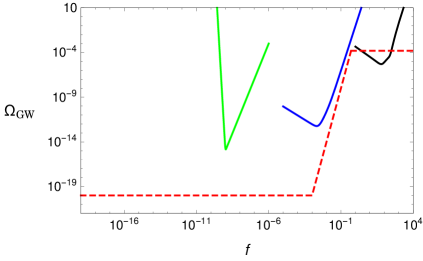
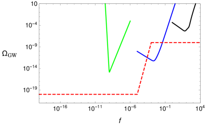
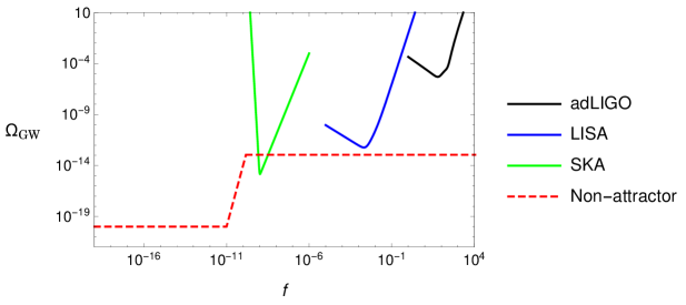
Figure 1: This figure shows qualitatively how primordial tensor modes get amplified during a non-attractor phase. They can contribute to the GW energy density $\Omega_{GW}$, and thus enter within the sensitivity curves for GW detectors in their appropriate frequency ranges (expressed in Hz). We model inflation as a pure de Sitter phase, during which a short period of non-attractor evolution occurs – whose starting time and duration depend on the model one considers – enhancing the tensor spectrum. We use formula (2.11), and assume for simplicity instantaneous transitions between attractor and non-attractor eras. Our conventions for the definition of the GW energy density $\Omega_{GW}$ are the same as in [84].

Such amplification of tensor fluctuations during a (typically short) non-attractor phase can lead to a very steep increase of the tensor spectrum as a function of frequency, once the amplitude of primordial tensor modes is transferred to the present cosmological epoch using standard formulae – see e.g. [84]. In Figure 1, we show how the spectrum of the superhorizon modes can be amplified to enter within the sensitivity curves for GW detectors, using formula (2.11), and assuming for simplicity instantaneous transitions between attractor and non-attractor eras. The figure is only indicative, because it does not take into account the transition phases during different epochs and, above all, does not take into consideration additional model-dependent constraints from amplification of scalar modes. In the next subsection we briefly review an example of a concrete realisation of a tensor dual to a slow-roll phase in single field inflation.

2.2 A concrete realisation in single field inflation

We now briefly review an explicit realisation of the mechanism of the previous subsection in a single field inflationary scenario, first presented in [1]. For convenience, we wish to find a single field inflationary model where the functions ${\cal F}_{T}$ and ${\cal G}_{T}$ introduced in the action (2.3) are directly proportional to the square of scalar field velocity $\dot{\phi}$ as

$${\cal F}_{T} \propto \frac{\dot{\phi}^{2}}{H_{0}^{2}}\,,\hskip 28.45274pt;\hskip 28.45274pt{\cal G}_{T}\,\propto\,\frac{\dot{\phi}^{2}}{H_{0}^{2}}\,,$$ (2.12)

during the entire phase of the inflationary evolution, which for simplicity we describe in terms of pure de Sitter evolution with constant Hubble parameter $H_{0}$. The scalar field follows a slow-roll evolution with constant velocity $\dot{\phi}\,=\,{\rm const}$ for most of the inflationary phase, but there is a brief phase of non-attractor evolution (whose duration is tunable in terms of the available parameters) during which $\dot{\phi}\propto 1/a^{3}$:

$$\dot{\phi}\,\propto\left\{\begin{array}[]{l}{\rm const}\hskip 28.45274pt{\text{during slow-roll phase}}\\ 1/a^{3}\hskip 28.45274pt{\text{during non-attractor phase}}\end{array}\right.$$

See Fig 2 for a representation of the scalar field time dependent profile. Plugging these scalar profiles into the expressions for the functions ${\cal F}_{T}$, ${\cal G}_{T}$ of eq (2.12) and recalling the definition of the pump field $z_{T}$, eq (2.6), it is easy to show that during the non-attractor phase we can use the tensor duality of eq (2.9), and the tensor power spectrum is enhanced by a factor $a^{6}(t)$ in this era (2.11). Indeed, such a scenario is conceptually similar to the model of Starobinsky [39], designed to enhance scalar fluctuations during non-attractor inflation (see also [59] and references therein).

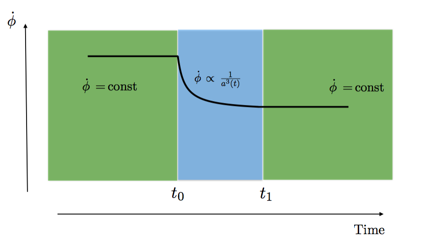
Figure 2: Behaviour of the scalar field derivative in our system.

The conditions described above can be realised if the scalar field has non-minimal couplings with gravity during inflation. We consider a scenario based on Horndeski theory of gravity, the most general scalar-tensor set-up with second order equations of motion, which is described by the Lagrangian

$${\cal L}_{\text{tot}} = {\cal L}_{2}+{\cal L}_{3}+{\cal L}_{4}+{\cal L}_{5}\,,$$ (2.14)

$${\cal L}_{2} = G_{2}\,\,,$$ (2.15)

$${\cal L}_{3} = -G_{3}\,\Box\phi\,\,,$$ (2.16)

$${\cal L}_{4} = G_{4}\,R+G_{4X}\left[\left(\Box\phi\right)^{2}-\left(\nabla_{\mu}\nabla_{\nu}\phi\right)^{2}\right]\,,$$ (2.17)

$${\cal L}_{5} = G_{5}\,G_{\mu\nu}\,\nabla^{\mu}\nabla^{\nu}\,\phi-\frac{G_{5X}}{6}\,\left[\left(\Box\phi\right)^{3}-3\Box\phi\,\left(\nabla_{\mu}\nabla_{\nu}\phi\right)^{2}+2\left(\nabla_{\mu}\nabla_{\nu}\phi\right)^{3}\right]\,.$$ (2.18)

The quantities $G_{a}\,=\,G_{a}(\phi,X)$ ($a=1,\dots 5$) are in principle arbitrary functions of the scalar field $\phi$ and

$$X\,=\,-\,\frac{1}{2}\,\partial_{\mu}\phi\partial^{\mu}\phi\,,$$ (2.19)

$R$ is the Ricci tensor, $G_{\mu\nu}$ is the Einstein tensor, and $G_{a\,X}=\partial G_{a}/\partial X$. For simplicity, in this work we focus on scenarios where a shift symmetry $\phi\to\phi+c$ is imposed, and the $G_{i}$ only depend on the kinetic function $X$. Inflation in scenarios based on Horndeski and Galileon Lagrangians have a long history, starting from [85] and the more general G-inflation [86, 75] models. Scenarios of ultra slow-roll, non-attractor G-inflation have been discussed in [87]. The quadratic Lagrangian for tensor fluctuations is described by our initial action (2.3) with

$${\cal F}_{T} = 2\left[G_{4}-X\,\ddot{\phi}\,G_{5X}\right]$$ (2.20)

$${\cal G}_{T} = 2\left[G_{4}-2\,X\,G_{4X}-X\,H_{0}\,\dot{\phi}\,G_{5X}\right]\,.$$ (2.21)

In [1] we showed that the conditions (2.12) can be realised by choosing the following structure for the functions $G_{a}(X)$

$$G_{2} = \rho X+\frac{\sqrt{2}\,H_{0}^{2}\,\alpha}{3}\,\sqrt{X}-\nu\,,\hskip 28.45274ptG_{3}\,=\,\frac{\sqrt{2}\,\delta}{3\,H_{0}}\,\sqrt{X}\,,$$

$$G_{4} = -\frac{\beta}{6H_{0}^{2}}\,X\,,\hskip 96.73918ptG_{5}\,=\,\frac{\sigma}{\sqrt{2}\,H_{0}^{3}}\,\sqrt{X}\,,$$ (2.22)

where the Greek letters are constant coefficients – which can be different during the three different phases of evolution summarised in Figure 2 – and $H_{0}$ is the constant Hubble parameter during inflation. We refer the reader to [1] for a detailed analysis of the system, with a quantitative discussion on the conditions necessary to avoid instability and to enhance the tensor power spectrum at superhorizon scales during the non-attractor phase. Notice that besides the tensor modes, scalar modes are also typically enhanced in these scenarios, although with a smaller amplitude [1].

3 Tensor non-Gaussianity in non-attractor inflation

The mechanism we analysed in the previous Section shows that it is possible to enhance the tensor power spectrum at small (interferometer) scales by exploiting the behaviour of the would-be decaying mode, which can grow in a regime of non-attractor inflation. An interesting feature of our mechanism is that there exists a tensor duality which allows us to obtain analytical expressions for the tensor power spectrum even in regimes that are far from a slow-roll period. In this Section, we study the tensor bispectrum, providing analytical expressions for this quantity during the non-attractor phase, and showing that the amplitude, shape and scale dependence of the tensor bispectrum can be different with respect to standard slow-roll inflation.

The tensor bispectrum is an interesting theoretical quantity which allows to discriminate between primordial and astrophysical sources of stochastic gravitational wave backgrounds (SGWB) [72]: if large tensor non-Gaussianity is detected, then it is likely that the SGWB has primordial origin, since an astrophysical GW background – formed by contributions from many unresolved sources – is likely to be Gaussian from the central limit theorem. The properties of the tensor bispectrum – shape, scale dependence, its value in the squeezed limit – are important for characterising the field content during inflation, and to further distinguish among different primordial sources that can amplify the tensor spectrum at interferometer scales [72].

Remarkably, the cubic action for tensor fluctuations around FRW in single field inflationary theories with second order equations of motion – the starting point for the computation of the bispectrum – has a simple structure, and contains only two contributions [88, 89]

$$S_{T}^{(3)} = \int{\rm d}t\,{\rm d}^{3}x\,a^{3}\,\left[\frac{\mathcal{F}_{T}}{4a^{2}}\left(h_{ik}h_{jl}-\frac{1}{2}h_{ij}h_{kl}\right)\partial_{k}\partial_{l}h_{ij}+\frac{\dot{\phi}XG_{5X}}{12}\dot{h}_{ij}\dot{h}_{jk}\dot{h}_{ki}\right],$$ (3.1)

$$= S_{T(\rm GR)}^{(3)}+S_{T(\rm new)}^{(3)}\,.$$

This action is obtained expanding the Horndeski Lagrangian density (2.14) up to cubic order in fluctuations, and the functions ${\cal F}_{T}$ and $G_{5}$ are given respectively in (2.20) and (2.18). The result of standard single field inflation with canonical kinetic terms is obtained setting ${\cal F}_{T}\,=\,1$ (recall that we choose units such that $M_{\rm pl}^{2}=1$). The structure of the first contribution, containing spatial derivatives only, is the same as the one obtained expanding the Ricci scalar at cubic order around a FRW background: this is the reason we denote it as $S_{T(\rm GR)}^{(3)}$. The second contribution, $S_{T(\rm new)}^{(3)}$, is instead specific to the Horndeski action: notice that it contains three time derivatives $\dot{h}_{ij}^{3}$, a feature to which we will return later. Tensor non-Gaussianity associated with the action (3.1) was studied in detail in a slow-roll regime in [88, 89], where it was found that the ‘GR’ term gives a bispectrum enhanced in the squeezed limit, while the ‘new’ contribution gives a bispectrum peaked in equilateral configurations. In this work, instead, we will work out the tensor non-Gaussianity during a transient non-attractor phase, finding quite different results.

3.1 Amplitude of tensor non-Gaussianity

We discuss the amplitude and some properties of tensor non-Gaussianity during an era of non-attractor inflation, which is dual to a slow-roll phase as explained in Section 2. For simplicity, we focus on the case where the background geometry is exactly described by a de Sitter universe, with constant Hubble parameter $H_{0}$ (in [1] we proved that the equations of motion admit this solution for the scale factor). We relegate all the technical details to Appendix A, and we discuss here the physical consequences of our computation of the tensor three point function in Fourier space during a non-attractor era. In order to express our results more concisely, we define two polarisation modes as (here, $e_{ij}^{(s)}$ is the polarization tensor with the helicity states $s=\pm$, satisfying $e_{ii}^{(s)}(\mathbf{k})=0=k_{j}e_{ij}^{(s)}(\mathbf{k})$. See Appendix A for more information regarding our conventions on the polarisation tensors)

$$\xi^{(s)}({\bf k})\equiv h_{ij}({\bf k})e^{*(s)}_{ij}({\bf k}),$$ (3.2)

which allow us to express the three point function in the non-attractor era as

$$\langle\xi^{(s_{1})}(\mathbf{k}_{1})\xi^{(s_{2})}(\mathbf{k}_{2})\xi^{(s_{3})}(\mathbf{k}_{3})\rangle = (2\pi)^{7}\delta({\bf k}_{1}+{\bf k}_{2}+{\bf k}_{3})\frac{\mathcal{P}^{(\rm end)^{2}}_{h}}{\Pi_{i}\leavevmode\nobreak\ k_{i}^{3}}\leavevmode\nobreak\ \bigg{(}\mathcal{A}^{s_{1}s_{2}s_{3}}_{(\rm new)}+\mathcal{A}^{s_{1}s_{2}s_{3}}_{(\rm GR)}\bigg{)}\,,$$ (3.3)

$$\equiv (2\pi)^{7}\,\delta({\bf k}_{1}+{\bf k}_{2}+{\bf k}_{3})\,B^{s_{1}s_{2}s_{3}}(\mathbf{k}_{i})\,.$$ (3.4)

Hence we define the tensor bispectrum $B^{s_{1}s_{2}s_{3}}(\mathbf{k}_{i})$ as the coefficient of the $\delta$-function in the previous expression, which depends on the momenta as well as on the polarisation indices.

Using (A.18), (A.27), the amplitudes

$$\mathcal{A}^{s_{1}s_{2}s_{3}}_{(\rm new),(\rm GR)}\equiv e^{*(s_{1})}_{i_{1}j_{1}}(\mathbf{k}_{1})e^{*(s_{2})}_{i_{2}j_{2}}(\mathbf{k}_{2})e^{*(s_{3})}_{i_{3}j_{3}}(\mathbf{k}_{3})\mathcal{A}^{(\rm new),(\rm GR)}_{i_{1}j_{i}i_{2}j_{2}i_{3}j_{3}}$$

can be calculated following the same methods of [89]. For our scenario, in the non-attractor regime, we find

$$\mathcal{A}^{s_{1}s_{2}s_{3}}_{(\rm new)} =\mathcal{A}^{(\rm new)}(k_{1},k_{2},k_{3})F(s_{1}k_{1},s_{2}k_{2},s_{3}k_{3})$$

$$\mathcal{A}^{s_{1}s_{2}s_{3}}_{(\rm GR)} =\mathcal{A}^{(\rm GR)}(k_{1},k_{2},k_{3})\frac{(s_{1}k_{1}+s_{2}k_{2}+s_{3}k_{3})^{2}}{2}F(s_{1}k_{1},s_{2}k_{2},s_{3}k_{3}),$$ (3.5)

where

$$F(x,y,z)=\frac{1}{64}\frac{1}{x^{2}y^{2}z^{2}}(x+y+z)^{3}(x-y+z)(x+y-z)(x-y-z).$$ (3.6)

$\mathcal{A}^{(\rm GR)}$ and $\mathcal{A}^{(\rm new)}$ are obtained in equations (A) and (A) respectively, which we rewrite here:

$$\mathcal{A}^{(\rm GR)} =-\frac{K}{64}\Bigg{[}\left(1-\frac{3}{K^{3}}\sum_{i\neq j}k_{i}^{2}k_{j}-\frac{6}{K^{3}}\Pi_{i}k_{i}\right)(-Ky_{\rm end})^{2}$$

$$\leavevmode\nobreak\ \leavevmode\nobreak\ \leavevmode\nobreak\ \leavevmode\nobreak\ \leavevmode\nobreak\ \leavevmode\nobreak\ \leavevmode\nobreak\ \leavevmode\nobreak\ \leavevmode\nobreak\ \leavevmode\nobreak\ \leavevmode\nobreak\ -\frac{\pi}{4}\left(1-\frac{4}{K^{3}}\sum_{i\neq j}k_{i}^{2}k_{j}-\frac{4}{K^{3}}\Pi_{i}k_{i}\right)(-Ky_{\rm end})^{3}+\dots\Bigg{]},$$ (3.7)

$$\mathcal{A^{(\rm new)}}=-\frac{3H\mu^{(\rm end)}}{16\mathcal{G}^{(\rm end)}_{T}} \Bigg{\{}\left(K^{3}-3\sum_{i\neq j}k_{i}^{2}k_{j}-6\leavevmode\nobreak\ \Pi_{i}k_{i}\right)$$

$$-\frac{1}{4}\Bigg{(}K^{3}-5\sum_{i\neq j}k_{i}^{2}k_{j}+\frac{2}{K^{2}}\sum_{i\neq j}k_{i}^{3}k_{j}^{2}\Bigg{)}(-Ky_{\rm end})^{2}\Bigg{\}}.$$ (3.8)

In these formulae, $K\,=\,k_{1}+k_{2}+k_{3}$,

$$\mu^{(\rm end)}\equiv\dot{\phi}^{(\rm end)}X^{(\rm end)}G_{5X}^{(\rm end)}$$

and the ‘end’ indicates the end of the non-attractor phase: our results then quantify the non-Gaussianity accumulated by the tensor modes during the non-attractor era. Before proceeding, some observations are in order:

• The squeezed limit of the bispectrum does not satisfy Maldacena’s consistency relations [61]. Indeed, computing the bispectrum of eq (3.4) for $s_{1}=s_{2}$ in the limit of squeezed isosceles triangles, we find

  $$B^{s_{1}s_{1}s_{3}}({\bf k}_{1},\,-{\bf k}_{1},\,{\bf k}_{3}\to 0) = \,\frac{\left({\cal P}_{h}^{({\rm end})}\right)^{2}}{32\,k_{1}^{3}\,k_{3}^{3}}\,\left[\frac{3\,H\mu^{(\rm end)}}{\mathcal{G}_{T}^{(\rm end)}}\left(1+\frac{(-k_{1}y_{\rm end})^{2}}{2}\right)+\frac{(-k_{1}y_{\rm end})^{2}}{2}\right]\,,$$

  while we find zero for $s_{1}\neq s_{2}$. Instead, Maldacena’s consistency relation (with our conventions) would read in this case

  $$B^{s_{1}s_{1}s_{3}}({\bf k}_{1},\,-{\bf k}_{1},\,{\bf k}_{3}\to 0)\,=\,\frac{3}{64\,k_{1}^{3}\,k_{3}^{3}}\,\left({\cal P}_{h}^{({\rm end})}\right)^{2}\,.$$

  This can be expected, since during the non-attractor era, besides the usual growing tensor mode, the would be tensor decaying mode is excited as well, and we are no longer working in a ‘single tensor’ adiabatic system where Maldacena’s arguments apply . By tuning the parameters of the model, this implies that the amplitude of the tensor bispectrum can be enhanced in the squeezed limit (see also [27, 28, 94, 95, 96] for different scenarios with enhanced squeezed tensor bispectrum), with potentially interesting phenomenological consequences that we shall discuss in Section 3.3.

• While the scenario studied so far is characterised by non-standard kinetic terms for the tensor sector, it is known that by performing a conformal followed by a disformal transformation the second order action for tensor modes – our eq. (2.3) – acquires the very same structure of the second order action of Einstein gravity around FRW homogeneous backgrounds [73]. On the other hand, the third order action we are considering here, eq (3.1), contains a piece with three time derivatives $\dot{h}_{ij}^{3}$ – an operator that cannot be recast into a pure ‘GR’ contribution via disformal/conformal transformations. This said, in Appendix B we show in detail that all our results remain the same also in an ‘Einstein frame’ with standard second order tensor action: the only difference is that in this frame the non-attractor phase corresponds to a short period of universe contraction.

• Our expressions for the tensor bispectrum contain a characteristic scale dependence with overall factors containing powers of $(-K\,y_{\rm end})$, that are distinctive of our scenario – being absent in other frameworks with large tensor non-Gaussianity. The explicit dependence on the time $y_{end}$ when the non-attractor phase ends is due to the fact that the bispectrum has been computed specifically at the end of the non-attractor phase. For simplicity, we assume that this era is immediately followed by a standard slow-roll inflation, where tensor modes and their statistics are frozen in a super-horizon regime. The overall scale dependence of the tensor bispectrum controlled by $K$ is also distinctive of our set-up. Similar situations have been encountered in the scalar sector, starting from the work [82], for models with non-standard cosmological expansion history, leading to interesting observables associated with scale-dependent non-Gaussianity (explored in general terms in [97, 98, 99]). A consequence of this fact is that non-Gaussianity depends on the scale and might be different at different interferometer scales (for example, LIGO-VIRGO and LISA): it would be interesting to further explore phenomenological consequences of this property, which goes beyond the scope of our work.

We now continue by estimating the amplitude of non-Gaussian signal. As a measure for the amount of non-Gaussianity, we use the following definition of the non-linearity parameter $f_{\rm NL}$, as in the works [88, 89]

$$\hat{f}^{s_{1}s_{2}s_{3}}_{\rm NL(\rm new),(\rm GR)}\equiv 30\frac{\mathcal{A}^{s_{1}s_{2}s_{3}}_{(\rm new),(\rm GR)}}{K^{3}}\bigg{\rvert}_{k_{1}=k_{2}=k_{3}},$$ (3.10)

which is analogous to the standard $f_{\rm NL}$ for the scalar curvature perturbation. Notice that the $f_{\rm NL}$ above is defined in terms of equilateral configurations for tensor bispectra, and its value depends on the polarisations. Using the definitions of the two amplitudes in (3.1), we find

$$\hat{f}^{s_{1}s_{2}s_{3}}_{\rm NL(\rm new)} =-\frac{45}{32}\leavevmode\nobreak\ \big{[}3+2(s_{1}s_{2}+s_{1}s_{3}+s_{2}s_{3})\big{]}\frac{\mathcal{A}^{(\rm new)}(K/3,K/3,K/3)}{K^{3}},$$ (3.11)

$$\hat{f}^{s_{1}s_{2}s_{3}}_{\rm NL(\rm GR)} =-\frac{5}{64}\big{[}21+20(s_{1}s_{2}+s_{1}s_{3}+s_{2}s_{3})\big{]}\frac{\mathcal{A}^{(\rm GR)}(K/3,K/3,K/3)}{K}.$$ (3.12)

The dependence of the non-linerity parameter on the polarization implies the following symmetry $\hat{f}^{++-}_{\rm NL(\rm new),(\rm GR)}=\hat{f}^{+--}_{\rm NL(\rm new),(\rm GR)}$ and $\hat{f}^{+++}_{\rm NL(\rm new),(\rm GR)}=\hat{f}^{---}_{\rm NL(\rm new),(\rm GR)}$ which follows from the fact that the interactions we consider do not violate parity. More concretely, we have

$$\hat{f}^{+++}_{\rm NL(\rm new)}=\frac{135}{512}\frac{H\mu^{(\rm end)}}{\mathcal{G}_{T}^{(\rm end)}}\left(1+\frac{5}{36}(-Ky_{\rm end})^{2}\right)$$ (3.13)

and

$$\hat{f}^{++-}_{\rm NL(\rm new)}=\frac{15}{512}\frac{H\mu^{(\rm end)}}{\mathcal{G}_{T}^{(\rm end)}}\left(1+\frac{5}{36}(-Ky_{\rm end})^{2}\right).$$ (3.14)

Similarly for $f^{s_{1}s_{2}s_{3}}_{\rm NL(\rm GR)}$ we have

$$\hat{f}^{+++}_{\rm NL(\rm GR)}=\frac{45}{4096}\leavevmode\nobreak\ (-Ky_{\rm end})^{2}\leavevmode\nobreak\ \bigg{[}1+\frac{\pi}{12}(-Ky_{\rm end})\bigg{]}$$ (3.15)

and

$$\hat{f}^{++-}_{\rm NL(\rm GR)}=\frac{5}{36864}\leavevmode\nobreak\ (-Ky_{\rm end})^{2}\leavevmode\nobreak\ \bigg{[}1+\frac{\pi}{12}(-Ky_{\rm end})\bigg{]}.$$ (3.16)

These results show that the $f_{\rm NL}$ parameter is generically positive during the non-attractor phase, similar to the case of contracting universes considered in [82]. Importantly, due to the strong scale dependence of the $f_{\rm NL(\rm GR)}$, $f_{\rm NL(\rm new)}$ dominates the bispectrum for $-k_{i}y_{\rm end}\ll 1$ and $H\mu^{(\rm end)}/\mathcal{G}_{T}^{(\rm end)}\sim\mathcal{O}(1)$. Recall that $\mathcal{G}_{T}\supset\mu H$, in particular

$$\mathcal{G}_{T}=2\left(G_{4}-2XG_{4X}-\mu H\right)$$ (3.17)

for the background model we discussed earlier. The expression above (3.17) indicates that we need accidental cancellations between the first two terms in $\mathcal{G}_{T}>0$ and $\mu H$ in order to ensure $H\mu/\mathcal{G}_{T}\gg 1$. We discuss in Appendix C a concrete scenario leading to large tensor non-Gaussianity within the framework we reviewed in Section 2.2.

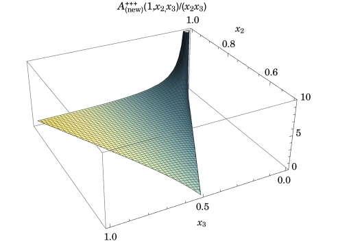
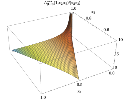
Figure 3: $\mathcal{A}^{+++}_{(\rm new)}(1,x_{2},x_{3})/(x_{2}x_{3})$ as a function of $x_{2}$ and $x_{3}$ where we set $H\mu^{\rm end}/\mathcal{G}_{T}^{\rm end}\to 1$ (Left). $\mathcal{A}^{+++}_{(\rm GR)}(1,x_{2},x_{3})/(x_{2}x_{3})$ as a function of $x_{2}$ and $x_{3}$ (Right). In both plots we normalized the amplitudes $\mathcal{A}^{+++}_{(\rm new)}$ and $\mathcal{A}^{+++}_{(\rm GR)}$ to unity for equilateral configurations $x_{2}=x_{3}=1$ and took $-Ky_{\rm end}=10^{-2}$.

3.2 Shape of tensor non-Gaussianity

We now study the shape of non-Gaussianity in our model. Since both of the amplitudes have non-trivial scale dependence, we examine the shape of the amplitudes  at fixed $-Ky_{\rm end}$. We focus on the dimensionless ratio $\mathcal{A}^{s_{1}s_{2}s_{3}}_{(\rm new),(\rm GR)}/(k_{1}k_{2}k_{3})$ of both amplitudes in (3.1) following the literature for scalar perturbations [100]. In particular, we will plot $\mathcal{A}^{s_{1}s_{2}s_{3}}_{(\rm new),(\rm GR)}/(k_{1}k_{2}k_{3})$ in the $x_{2}-x_{3}$ plane where $x_{j}\equiv k_{j}/k_{1}$ with $j\neq 1$ by restricting ourselves to the range $1-x_{2}\leq x_{3}\leq x_{2}$. Note that the first inequality follows from the triangle inequality whereas the latter allows us to avoid plotting the same configuration twice. The non-Gaussian amplitudes $\mathcal{A}^{+++}_{(\rm new)}/(k_{1}k_{2}k_{3})$ and $\mathcal{A}^{+++}_{(\rm GR)}/(k_{1}k_{2}k_{3})$ are shown in Figure 3. We see that both the interaction terms in (3.1) give rise to non-Gaussianity that peaks in the squeezed limit. This result is in contrast with the slow-roll case where the new contribution peaks in the equilateral configuration. This difference is due to the fact that during the non-attractor phase, the fluctuations in $h_{ij}$ keeps growing outside the horizon due to the dynamics of the would be decaying mode, i.e. $\dot{h}_{ij}=3Hh_{ij}$ and therefore the non-Gaussian amplitude peaks when one of the wave numbers is small, corresponding to the squeezed-triangle limit. In the standard attractor slow-roll background however, tensor fluctuations freeze on large scales, $\dot{h}_{ij}\to 0$ and therefore only wave-numbers comparable to the size of the horizon can contribute to the non-Gaussianity for the interaction proportional to the time derivatives of $h_{ij}$ in (3.1).

3.3 Interferometer response function for anisotropic tensor power spectrum

As we explained in Subsection 3.1, our system does not satisfy Maldacena consistency relations: the squeezed limit of the bispectrum can be enhanced by the contributions of the would be decaying tensor mode. This means that we can develop a scenario where at the same time we have a large tensor power spectrum at interferometer scales, accompanied by enhanced squeezed tensor non-Gaussianity. In this subsection, we start with a brief ‘theory’ part to connect the squeezed limit of the tensor bispectrum with a quadrupolar anisotropy of the tensor power spectrum; we then continue with a discussion on possible ways to detect an anisotropic gravitational wave power spectrum with ground based interferometers, building on the results of [101].

Theory: A large non-Gaussianity in the squeezed limit can induce couplings between modes at different scales: the tensor power spectrum is modulated by long tensor modes that induce large scale anisotropies. This fact has been explored in several contexts, mainly in the scalar, but also in the tensor sector: see e.g. [102, 103, 104, 105]. Other scenarios that can induce large tensor non-Gaussianity in the squeezed limit, by violating the adiabaticity condition in the tensor sector, are supersolid inflation [25, 26, 27, 28, 33, 32], bigravity or higher spin theories [35, 36, 94, 37, 95, 96]; our considerations can apply to these cases as well.

When focussing on the ‘GR’ operator of action, one finds that squeezed non-Gaussianity induces a quadrupolar anisotropy in the tensor power spectrum, with (see e.g. [106, 36])

$${\cal P}_{h}({\bf{k}},\,{\bf x})\,=\,{\cal P}_{h}^{(0)}({{k}})\,\left[1+{\cal Q}_{ij}({\bf{k}},\,{\bf x})\,\hat{k}_{i}\hat{k}_{j}\right]$$ (3.18)

and

$${\cal Q}_{ij}({\bf{k}},\,{\bf x})\,=\,\sum_{s_{1},s_{2}}\int_{L^{-1}}\,\frac{d^{3}q}{(2\pi)^{3}}\,e^{i\,{\bf q}\,{\bf x}}\,\left(\frac{B^{s_{1}s_{1}s_{2}}({\bf q},\,{\bf k},\,-{\bf q}-{\bf k})}{P_{h}(q)P_{h}(k)}\right)\,h_{\bf q}e_{ij}^{(s_{2})}({\bf q})\,.$$ (3.19)

We expect that the modulation (3.18) of the tensor power spectrum arises in any scenario with enhanced squeezed tensor non-Gaussianity. The integral defining the anisotropy parameter is evaluated in a patch centered at the position ${\bf x}$ and spans over long tensor modes with momenta within the non-attractor phase, corresponding to scales well larger than the gravitational wave wavelengths under consideration (see e.g. Section 4.4 of [36]). Being dependent on a linear combination of the polarization tensors $e_{ij}^{(s)}$, the quantity $Q_{ij}$ is traceless. It is convenient to define the squeezed limit of the bispectrum as

$$\lim_{{\bf q}\to 0}\frac{B^{s_{1}s_{1}s_{2}}({\bf k},\,-{\bf k},{\bf q})}{P_{h}(q)P_{h}(k)}\,=\,\frac{3}{64}+\hat{f}_{\rm NL}^{\rm sqz}\,,$$ (3.20)

where the quantity $\hat{f}_{\rm NL}^{\rm sqz}$ parameterises the deviation from the Maldacena’s consistency conditions. In our case, the quantity $\hat{f}_{\rm NL}^{\rm sqz}$ can be read from eq (LABEL:sqxbisf). The anisotropy parameter ${\cal Q}_{ij}$ is determined in a statistical sense, averaging over many large patches. Its average equal to zero, and its variance results (see e.g. [106, 36])

$$\langle{\cal Q}_{ij}({\bf k})\,{\cal Q}_{mn}({\bf k})\rangle = \frac{\pi}{20}\left(\delta_{im}\delta_{jn}+\delta_{in}\delta_{jm}-\frac{2}{3}\delta_{ij}\delta_{mn}\right)\,\int\frac{dk}{k}\,\big{|}\hat{f}_{\rm NL}^{\rm sqz}\big{|}^{2}\,{\cal P}_{h}^{2}\,,$$ (3.21)

$$\simeq \left(\delta_{im}\delta_{jn}+\delta_{in}\delta_{jm}-\frac{2}{3}\delta_{ij}\delta_{mn}\right)\big{|}\hat{f}_{\rm NL}^{\rm sqz}\big{|}^{2}\,{\cal P}_{h}^{2}\,\Delta N$$ (3.22)

where in the last line we specialised for simplicity to the case of scale invariant power-spectrum and squeezed $f_{\rm NL}^{\rm sqz}$, and $\Delta N$ indicates the number of e-folds of cosmological evolution associated with the non-attractor era. The value of ${\cal P}_{h}$ in the previous formula indicates the magnitude of the tensor power spectrum at the end of non-attractor, which can be much larger than its value during the initial phase of slow-roll. Assuming that the magnitude of tensor spectrum is of order $\sim 10^{-14}$ at large scales, and it receives a $10^{10}$ enhancement during three e-folds of non-attractor inflation (using eq (2.11)), we learn that $f_{\rm NL}^{\rm sqz}\sim 100$ is sufficient to give a value for $\sqrt{\langle{\cal Q}_{ij}^{2}\rangle}$ of the order of a few percent (but $\sqrt{\langle{\cal Q}_{ij}^{2}\rangle}$ can be larger depending on the magnitude of tensor non-Gaussianity).

These results imply that the size of the anisotropy parameter can be a probe of the squeezed tensor bispectrum. We now outline a possible way to test such quantity with ground based interferometers .

Connection with gravitational wave experiments: The possibility of detecting anisotropies in a SGWB has started with the work [101], that derived the formalism necessary to quantitatively address the subject. The motivation for such investigations is to detect signals from a stochastic background due to astrophysical sources that can generate multipolar anisotropies. On the other hand, the formalism of [101] is sufficiently general and can be used with little changes also to investigate tensor anisotropies from the early universe. We apply the formulae and arguments of [101] to analyse tensor power spectra with a quadrupolar anisotropic structure as in eq (3.18). We focus for simplicity on analysing the response function for a single Michelson ground-based interferometer (see [108, 109] for reviews).

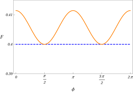
Figure 4: Modulation of the response function $F$ of eq (3.26) as the interferometer rotates an angle $\phi$ around an axis aligned with one of the interferometer arms. We assume that this arm points along the earth’s rotation axis, and we choose a reference frame so that it corresponds to the direction $\hat{x}$. The dashed blue line shows the case with no anisotropy, $Q_{ij}=0$, whereas the orange line shows the case with one component $Q_{33}\,=\,-Q_{11}\,=\,0.1$ turned on.

The total signal detected by an interferometer can decomposed as $S(t)\,=\,s(t)+n(t)$, with $n(t)$ the noise and $s(t)$ the contribution due to the gravitational wave. The relation between $s(t)$ and the mode $h_{ij}$ can be written as [108]

$$s(t)\,=\,{D}^{ij}\,h_{ij}(t)\,,$$ (3.23)

with ${D}_{ij}$ the detector tensor. For ground-based interferometers with arm directions $\hat{u}$ and $\hat{v}$ it reads

$${D}^{ij}\,=\,\frac{1}{2}\,\left(\hat{u}^{i}\hat{u}^{j}-\hat{v}^{i}\hat{v}^{j}\right)\,.$$ (3.24)

We introduce the detector pattern function

$$F^{\lambda}({\bf k})\,=\,D^{ij}\,e^{(\lambda)}_{ij}({\bf k})\,.$$ (3.25)

The single detector response function, as defined for example in Section 3 of [108] is the proportionality constant $F$ between the equal time 2pt function of the ground-based interferometer signal and the integral over frequencies of the amplitude of the primordial power spectrum ${\cal P}^{(0)}$. Using the techniques developed in [101], we find that the response function reads in our case

$$F\,=\,\frac{2}{5}-\frac{16}{35}\,{\cal Q}_{ij}{D}_{ik}D_{kj}\,.$$ (3.26)

The first contribution $2/5$ is the well known response function for an isotropic SGWB for a single, ground-based Michelson interferometer (see [108], Section 3). The additional contribution is instead new, and contains the anisotropic contributions of (3.18) to the interferometer response function: notice that it depends on the detector tensor ${D}_{ij}$.

As pointed out in [101], a response function as eq (3.26) can lead to a diurnal modulation of a ground-based interferometer signal, since the interferometer arms change orientation with respect to the anisotropy parameter ${\cal Q}_{ij}$ as the earth rotates around its axis. As a representative example, we plot in Fig 4 the modulation of the interferometer response function as the interferometer arms make a full rotation around the axis of rotation of the earth, when some of the components of the anisotropy parameter ${\cal Q}_{ij}$ is turned on. From the figure we learn that if we can probe percent variations of the interformeter response function – corresponding to diurnal modulations of the same order in the stochastic background – then we can probe anisotropies of the same magnitude: they correspond to values of $f_{\rm NL}^{\rm sqz}$ of the order of one hundred, which can be achieved in the model we are considering (see Appendix C).

It would be very interesting to study quantitatively whether current and future ground-based interferometers can set constraints on the size of $Q_{ij}$ for realistic values of $\hat{f}_{\rm NL}^{\rm sqz}$, by studying correlations among signals from different instruments in the presence of the primordial quadrupolar asymmetry, and by computing the corresponding signal-to-noise ratio. We plan to further develop these topics in a future publication.

4 Conclusions

We investigated the consequences of a non-attractor phase of cosmological evolution for the dynamics of primordial tensor modes, focussing on the properties of primordial tensor non-Gaussianity in scenarios with non-minimal couplings of gravity to the scalar sector. Thanks to a tensor duality, we have been able to analytically compute the properties of the tensor bispectrum during this phase. We have shown that the tensor bispectrum is enhanced in the squeezed limit with respect to standard slow-roll scenarios, and can parametrically violate Maldacena’s consistency relations. Moreover, tensor non-Gaussianity exhibits a scale dependence characteristic of our set-up, that can help to distinguish our model from other scenarios with large tensor non-Gaussianity. Squeezed tensor non-Gaussianity induces a characteristic quadrupolar anisotropy on the power spectrum of the stochastic background of primordial tensor perturbations. To make contact with gravitational wave experiments, we discussed the response function of a ground based Michelson interferometer to a gravitational wave background with such a feature.

Much work is left for the future. It would be interesting to apply our approach to more general scenarios then the ones considered so far, including theories of Beyond Horndeski or DHOST [110, 111, 112, 113, 114]. This would also allow one to study in more general terms the transition phase between attractor and non-attractor, and related possible instabilities associated with violations of energy conditions (see the discussion in the Appendix of [1]). At the phenomenological level, it would be important to further investigate to what extent gravitational wave experiments can probe the quadrupolar anisotropy in the tensor power spectrum induced by squeezed non-Gaussianity, by computing the corresponding signal-to-noise ratio for actual experiments, and relating it to the size of non-Gaussian observables. We plan to return on these topics soon.

Appendix A Technical appendix:
computation of two-point and three-point functions for tensor modes

In this Appendix, we go through the technical details of the results we discuss in the main text. We start showing that tensor duality allows us to obtain an analytical expression for tensor mode functions during the non-attractor era dual to a slow-roll phase: this is the basic ingredient we need for then analytically evaluating two point and three point functions in the non-attractor regime. For definiteness, the set-up we have in mind to realise this scenario is the same of Subsection 2.2, first discussed in [1]. In this case,

$${\cal F}_{T} \propto 1/a^{6}\hskip 28.45274ptc_{T}^{2}\,=\,{\cal F}_{T}/{\cal G}_{T}\,\propto\,{\rm constant}\hskip 28.45274pt{\text{ during non-attractor phase}}\,,$$ (A.1)

$${\cal F}_{T} \propto {\rm constant}\hskip 8.5359ptc_{T}^{2}\,=\,{\cal F}_{T}/{\cal G}_{T}\,\propto\,{\rm constant}\hskip 28.45274pt{\text{ during slow-roll phase}}\,.$$ (A.2)

We start by discussing the computation of the quadratic case, leading to the tensor power spectrum. To investigate the behavior of the tensor fluctuations, we define the canonically normalized tensor fluctuation $v_{ij}=z_{T}h_{ij}$ to re-write the leading order action (2.3) as

$$S_{T}^{(2)}\,=\,\frac{1}{2}\,\int{\rm d}y\,{\rm d}^{3}x\,\left[\left(v^{\prime}_{ij}\right)^{2}-\,\left(\vec{\nabla}v_{ij}\right)^{2}+\frac{z_{T}^{\prime\prime}}{z_{T}}\,v_{ij}^{2}\right]\,.$$ (A.3)

Using the expression (2.10), this leads to the following equation of motion in Fourier space

$${v_{\bf k}^{\prime\prime}+\left(k^{2}-\frac{2}{y^{2}}\right)v_{\bf k}=0,}$$ (A.4)

where we have used the following expansion for the canonical tensor perturbation

$$v_{ij}(y,\mathbf{k})=\sum_{s}e_{ij}^{(s)}(\mathbf{k})\bigg{[}v_{\mathbf{k}}(y)a_{s}(\mathbf{k})+v^{*}_{-\mathbf{k}}(y)a_{s}^{\dagger}(-\mathbf{k})\bigg{]}.$$ (A.5)

Here, $e_{ij}^{(s)}$ is the polarization tensor with the helicity states $s=\pm$, satisfying $e_{ii}^{(s)}(\mathbf{k})=0=k_{j}e_{ij}^{(s)}(\mathbf{k})$. Our normalisation is

$$e_{ij}^{(s)}(\mathbf{k})e_{ij}^{*(s^{\prime})}(\mathbf{k})=\delta_{ss^{\prime}},$$ (A.6)

and we choose the phase so that the following relations hold:

$$e_{ij}^{*(s)}(\mathbf{k})=e_{ij}^{(-s)}(\mathbf{k})=e_{ij}^{(s)}(-\mathbf{k}).$$ (A.7)

The commutation relation for the creation and annihilation operators is

$$[a_{s}(\mathbf{k}),a_{s^{\prime}}^{\dagger}(\mathbf{k}^{\prime})]=(2\pi)^{3}\delta_{ss^{\prime}}\delta(\mathbf{k}-\mathbf{k}^{\prime}).$$ (A.8)

The mode equation in (A.4) implies that the power spectrum of the fluctuations $v_{\bf k}$ is scale invariant on large scales. In order to see this, we note the solution to the differential equation in (A.4) that reduces to the adiabatic vacuum on small scales which reads

$${v_{\bf k}(y)=\frac{1}{\sqrt{2k}}\left(1-\frac{i}{ky}\right)e^{-iky}},$$ (A.9)

so that $\mathcal{P}_{h}\sim k^{3}|v_{k}|^{2}\propto k^{0}$ in the limit $-ky\to 0$, as anticipated. Using (A.9) and the formulae for $z_{T}$, we write the solution to the original tensor mode function by using $h_{\bf k}\equiv v_{\bf k}/z_{T}$,

$$h_{\bf k}(y)=\frac{i\sqrt{2}H}{\sqrt{c_{T}\mathcal{F}_{T}k^{3}}}\leavevmode\nobreak\ (1+iky)\leavevmode\nobreak\ e^{-iky},$$ (A.10)

which essentially has the same form as the one in the slow-roll approximation (see eq (11) of [89]), although in this case ${\cal F}_{T}$ is strongly time dependent, as discussed in Section 2.2 of the main text. Indeed, $\mathcal{F}_{T}$ is evolving rapidly as $\propto a^{-6}$ during the non-attractor regime contrary to the case in slow-roll where $\mathcal{F}_{T}\simeq$ constant, see eqs (2.12).

The two point function and the tensor power spectrum

Starting from the two point function of tensor modes in Fourier space, the power spectrum of tensor fluctuations can be defined by $\mathcal{P}_{h}=(k^{3}/2\pi^{2})\mathcal{P}_{ij,ij}$ using the following expressions

$$\langle h_{ij}(\mathbf{k})h_{kl}(\mathbf{k}^{\prime})\rangle = (2\pi)^{3}\delta(\mathbf{k}+\mathbf{k}^{\prime})\mathcal{P}_{ij,kl}(\mathbf{k}),$$ (A.11)

$$\mathcal{P}_{ij,kl}(\mathbf{k}) = |h_{\mathbf{k}}|^{2}\Pi_{ij,kl}(\mathbf{k}),$$ (A.12)

where

$$\Pi_{ij,kl}(\mathbf{k})=\sum_{s}e_{ij}^{(s)}(\mathbf{k})e_{kl}^{*(s)}(\mathbf{k}).$$ (A.13)

We learn that on super horizon scales $-ky\to 0$, one still gets a scale invariant power spectrum of primordial tensor fluctuations during the non-attractor phase.

$$\mathcal{P}_{h}=\lim_{-ky\to 0}\frac{k^{3}}{2\pi^{2}}2|h_{\bf k}|^{2}=\frac{2}{\pi^{2}}\frac{H^{2}}{\mathcal{F}_{T}c_{T}}.$$ (A.14)

However, since the tensor kinetic term evolves as $\mathcal{F}_{T}\propto a^{-6}$, the amplitude of the power spectrum grows on super-horizon scales and therefore it has to be evaluated at the end of the non-attractor era. These result shows an agreement with what one would expect from the duality arguments discussed in [58], namely the power spectrum grows on superhorizon scales while it preserves a scale invariant form.

The three point function and the tensor bispectrum

The tensor bispectrum can be computed by employing the in-in formalism (see e.g. [115]), starting from the three point function in Fourier space

$$\langle h_{i_{1}j_{1}}(\mathbf{k}_{1})h_{i_{2}j_{2}}(\mathbf{k}_{2})h_{i_{3}j_{3}}(\mathbf{k}_{3})\rangle$$

$$=-i\int^{t}_{t_{i}}{\rm d}t^{\prime}\leavevmode\nobreak\ \langle\leavevmode\nobreak\ \left[h_{i_{1}j_{1}}(t,\mathbf{k}_{1})h_{i_{2}j_{2}}(t,\mathbf{k}_{2})h_{i_{3}j_{3}}(t,\mathbf{k}_{3}),H_{\rm int}(t^{\prime})\right]\leavevmode\nobreak\ \rangle,$$ (A.15)

where $t_{i}$ is some early time when the perturbation is well inside the sound horizon and the interaction Hamiltonian is given by $H_{\rm int}(t)=-\int{\rm d}^{3}x\leavevmode\nobreak\ \mathcal{L}_{T}^{(3)}$. We find it convenient to work with the time coordinate $y$ in evaluating the three point function. We express all the time dependent quantities with respect to the time when the non-attractor era ends, $y_{\rm end}$. Using (A.10), the mode functions therefore take the following form

$$h_{\bf k}(y)=\frac{i\sqrt{2}H}{\sqrt{c_{T}\mathcal{F}_{T}^{(\rm end)}k^{3}}}\leavevmode\nobreak\ (1+iky)\leavevmode\nobreak\ e^{-iky}\left(\frac{y_{\rm end}}{y}\right)^{3},$$ (A.16)

where ⁽⁰⁾ denotes the value of the quantity at the beginning of the non-attractor era. Using the expansions in (A.5) (and noting $h_{ij}=v_{ij}/z_{T}$), we take the commutators in (A) by taking into account the relations between the polarization tensors (A.6),(A.7) and (A.8).

This procedure yields to the following expression for three point function,

$$\langle h_{i_{1}j_{1}}(\mathbf{k}_{1})h_{i_{2}j_{2}}(\mathbf{k}_{2})h_{i_{3}j_{3}}(\mathbf{k}_{3})\rangle$$

$$=(2\pi)^{3}\delta({\bf k}_{1}+{\bf k}_{2}+{\bf k}_{3})\leavevmode\nobreak\ \mathcal{T}^{(\alpha)}_{i_{1}j_{i}i_{2}j_{2}i_{3}j_{3}}\bigg{(}2\leavevmode\nobreak\ {\rm Im}[\leavevmode\nobreak\ \mathcal{I}^{(\alpha)}(y)\leavevmode\nobreak\ ]\bigg{)},$$ (A.17)

where the form of tensorial part $\mathcal{T}^{(\alpha)}$ and the function $\mathcal{I}^{(\alpha)}(y)$ depends on the interaction term under consideration in the third order action (3.1), denoted by the superscript $\alpha\,=\,\left({\rm GR},{\rm new}\right)$.

$\bullet$ The ‘GR’ contribution

We begin our calculations by the first term in the interaction Hamiltonian $H_{\rm int}(t)=-\int{\rm d}^{3}x\leavevmode\nobreak\ \mathcal{L}_{T}^{(3)}$, using the interaction Lagrangian (3.1) which we denote by $\alpha\to{\rm GR}$. In this case the tensorial part is given by

$$\mathcal{T}_{i_{1}j_{1}i_{2}j_{2}i_{3}j_{3}}^{({\rm GR})}=\bigg{\{}\Pi_{i_{1}j_{1},ik}(\mathbf{k}_{1})\Pi_{i_{2}j_{2},jl}(\mathbf{k}_{2})\bigg{[}k_{3k}k_{3l}\Pi_{i_{3}j_{3},ij}(\mathbf{k}_{3}) - \frac{1}{2}k_{3i}k_{3k}\Pi_{i_{3}j_{3},jl}(\mathbf{k}_{3})\bigg{]}$$ (A.18)

$$+ 5\leavevmode\nobreak\ {\rm perms}\leavevmode\nobreak\ {\rm of}\leavevmode\nobreak\ 1,2,3\leavevmode\nobreak\ \bigg{\}}.$$

where recall the definition of the four-index tensor $\Pi$ in eq (A.13). Since the tensor modes evolve outside the horizon during the non-attractor regime, we need to evaluate the function $\mathcal{I}$ (and hence the bispectrum) at the end of the non-attractor era beyond which we assume the mode functions (as well as time dependent quantities such as ${\mathcal{F}}_{T}$) freeze-out, since we return into a standard slow-roll phase. We are therefore interested in the following expression

$$\mathcal{I}^{(\rm GR)}=h_{\bf k_{1}}(y_{\rm end})h_{\bf k_{2}}(y_{\rm end})h_{\bf k_{3}}(y_{\rm end})\int_{-\infty}^{y_{\rm end}}{\rm d}y^{\prime}\leavevmode\nobreak\ \frac{a^{2}(y^{\prime}){\mathcal{F}}_{T}(y^{\prime})}{4\leavevmode\nobreak\ c_{T}}\leavevmode\nobreak\ h^{*}_{\bf k_{1}}(y^{\prime})h^{*}_{\bf k_{2}}(y^{\prime})h^{*}_{\bf k_{3}}(y^{\prime}),$$ (A.19)

where we take $y_{i}\to-\infty$ to ensure all modes of interest are inside the horizon initially and $y_{\rm end}$ denotes the end of non-attractor era. Noting the behavior of the mode functions in (A.10) and of the tensor kinetic function ${\mathcal{F}}_{T}\propto y^{6}$ during the non-attractor era, the function $\mathcal{I}^{(\rm GR)}$ contains integrals of the following form

$$\mathcal{C}^{(\alpha)}_{p}=\int_{\infty}^{x_{\rm end}}{\rm d}x^{\prime}\leavevmode\nobreak\ (x^{\prime})^{-p}\leavevmode\nobreak\ e^{-ix^{\prime}},$$ (A.20)

where we defined $x^{\prime}\equiv-Ky^{\prime}$ with $K=\sum_{i}k_{i}$ and $|{\bf k_{i}}|=k_{i}$. For the GR contribution we are focussing on, $p$ is a positive integer with the following possible values, $p=\{5,4,3,2\}$. The result of the integration can be expressed in terms of the incomplete Gamma functions,

$$\mathcal{C}^{(\alpha)}_{p}=-(-i)^{1-p}\leavevmode\nobreak\ \Gamma(1-p,ix_{\rm end})$$ (A.21)

which has the following series expansion for negative integer values of its first argument

$$\Gamma(-m,z)=\frac{1}{m!}\left(\frac{e^{-z}}{z^{m}}\sum_{k=0}^{m-1}(-1)^{k}(m-k-1)!\leavevmode\nobreak\ z^{k}+(-1)^{m}\leavevmode\nobreak\ \Gamma(0,z)\right).$$ (A.22)

The results above are valid as far as we are away from the origin $x_{\rm end}=0$ but diverges as $x_{\rm end}\to 0$. In the following, we will express our results for small but non-zero value of $x_{\rm end}\equiv-Ky_{\rm end}<1$. Moreover, notice that the incomplete Gamma $\Gamma(0,z)$ (also known as the exponential integral $E_{1}(z)$) admits the following useful power series expansion in terms of elementary functions,

$$\Gamma(0,z)=-\gamma_{E}-\ln(z)-\sum_{k=1}^{\infty}\frac{(-z)^{k}}{k\leavevmode\nobreak\ k!},$$ (A.23)

where $\gamma_{E}$ is the Euler-Mascheroni constant. Following the discussion above, we use (A.21) with (A.22) and (A.23) to present our results at next to leading order in $-Ky_{\rm end}<1$. Keeping in mind the full expression in (A.19), we thus have

$$2\leavevmode\nobreak\ {\rm Im}[\mathcal{I}^{(\rm GR)}] =\frac{(2\pi)^{4}\mathcal{P}_{h}^{(\rm end)^{2}}}{\Pi_{i}\leavevmode\nobreak\ k_{i}^{3}}$$

$$\leavevmode\nobreak\ \leavevmode\nobreak\ \times-\frac{K}{64}\Bigg{[}\left(1-\frac{3}{K^{3}}\sum_{i\neq j}k_{i}^{2}k_{j}-\frac{6}{K^{3}}\Pi_{i}k_{i}\right)(-Ky_{\rm end})^{2}$$

$$\leavevmode\nobreak\ \leavevmode\nobreak\ \leavevmode\nobreak\ \leavevmode\nobreak\ \leavevmode\nobreak\ \leavevmode\nobreak\ \leavevmode\nobreak\ \leavevmode\nobreak\ \leavevmode\nobreak\ \leavevmode\nobreak\ \leavevmode\nobreak\ \leavevmode\nobreak\ -\frac{\pi}{4}\left(1-\frac{4}{K^{3}}\sum_{i\neq j}k_{i}^{2}k_{j}-\frac{4}{K^{3}}\Pi_{i}k_{i}\right)(-Ky_{\rm end})^{3}\Bigg{]},$$ (A.24)

where we made use of the expression for the power spectrum in (A.14) evaluated at the end of the non-attractor era. With these ingredients, we can express the tensor three point function associated with the ‘GR’ contribution as

$$\langle h_{i_{1}j_{1}}(\mathbf{k}_{1})h_{i_{2}j_{2}}(\mathbf{k}_{2})h_{i_{3}j_{3}}(\mathbf{k}_{3})\rangle=(2\pi)^{7}\delta({\bf k}_{1}+{\bf k}_{2}+{\bf k}_{3})\frac{\mathcal{P}^{(\rm end)^{2}}_{h}}{\Pi_{i}\leavevmode\nobreak\ k_{i}^{3}}\leavevmode\nobreak\ \mathcal{A}^{(\rm GR)}_{i_{1}j_{i}i_{2}j_{2}i_{3}j_{3}},$$ (A.25)

where we defined $\mathcal{A}^{(\rm GR)}_{i_{1}j_{i}i_{2}j_{2}i_{3}j_{3}}\equiv\mathcal{A^{(\rm GR)}}(k_{1},k_{2},k_{3})\leavevmode\nobreak\ \mathcal{T}^{(\rm GR)}_{i_{1}j_{i}i_{2}j_{2}i_{3}j_{3}}$ with $\mathcal{T}^{(\rm GR)}$ given in eq (A.18),

$$\mathcal{A}^{(\rm GR)} =-\frac{K}{64}\Bigg{[}\left(1-\frac{3}{K^{3}}\sum_{i\neq j}k_{i}^{2}k_{j}-\frac{6}{K^{3}}\Pi_{i}k_{i}\right)(-Ky_{\rm end})^{2}$$

$$\leavevmode\nobreak\ \leavevmode\nobreak\ \leavevmode\nobreak\ \leavevmode\nobreak\ \leavevmode\nobreak\ \leavevmode\nobreak\ \leavevmode\nobreak\ \leavevmode\nobreak\ \leavevmode\nobreak\ \leavevmode\nobreak\ \leavevmode\nobreak\ -\frac{\pi}{4}\left(1-\frac{4}{K^{3}}\sum_{i\neq j}k_{i}^{2}k_{j}-\frac{4}{K^{3}}\Pi_{i}k_{i}\right)(-Ky_{\rm end})^{3}+\dots\Bigg{]},$$ (A.26)

and dots indicates sub-leading terms higher order in $-Ky_{\rm end}$. The amplitude $\mathcal{A}^{(\rm GR)}$ shows the scale dependence of the non-Gaussianity parametrized by the powers of $-Ky_{\rm end}<1$ during the non-attractor era.

$\bullet$ The ‘new’ contribution

In a similar fashion, we now move on to calculate the contribution to the tensor three point function from the second term in the interaction Hamiltonian (see e.g. (3.1)). Following the same steps as we did for the previous term, we write the three point function in the same form as in (A) with

$$\mathcal{T}_{i_{1}j_{1}i_{2}j_{2}i_{3}j_{3}}^{({\rm new})}=\Pi_{i_{1}j_{1},ij}(\mathbf{k}_{1})\Pi_{i_{2}j_{2},jk}(\mathbf{k}_{2})\Pi_{i_{3}j_{3},kl}(\mathbf{k}_{3})$$ (A.27)

and

$$\mathcal{I}^{(\rm new)}=-h_{\bf k_{1}}(y_{\rm end})h_{\bf k_{2}}(y_{\rm end})h_{\bf k_{3}}(y_{\rm end})\int_{-\infty}^{y_{\rm end}}{\rm d}y^{\prime}\leavevmode\nobreak\ \frac{c_{T}^{2}a\dot{\phi}XG_{5X}}{2}\leavevmode\nobreak\ h^{*^{\prime}}_{\bf k_{1}}(y^{\prime})h^{*^{\prime}}_{\bf k_{2}}(y^{\prime})h^{*^{\prime}}_{\bf k_{3}}(y^{\prime}).$$ (A.28)

Here a prime on the mode functions denotes a time derivative with respect to their argument $y^{\prime}$. We note that since the integral contains these time derivatives, the calculation of the 3-pt function associated with this contribution is more involved compared to the previous case. In order to deal with the integral in (A.28), we note the time derivative of the complex conjugated mode function as

$$h^{*^{\prime}}_{\bf k}(y)=-\frac{i\sqrt{2}H}{\sqrt{c_{T}\mathcal{F}_{T}^{(\rm end)}k^{3}}}\left(\frac{y_{\rm end}}{y}\right)^{3}\leavevmode\nobreak\ \left\{-\frac{3}{y}(1-iky)+k^{2}y\right\}\leavevmode\nobreak\ e^{iky},$$ (A.29)

which reflects the rapid change of the mode functions after horizon crossing ($-ky\to 0$). Noting the time dependence of the functions inside the integral, i.e. $\dot{\phi}\propto a^{-3}$, $X\propto a^{-6}$ and $G_{5X}\propto a^{3}$, we see that we need to deal with integrals that has the same form as in (A.20) with $p=\{7,6,5,4,3,2,1\}$. Therefore, repeating the same steps as we did for the “GR” term, we obtain the following results for $2{\rm Im}[\mathcal{I}^{(\rm new)}]$ at next to leading order in $-Ky_{\rm end}$,

$$2\leavevmode\nobreak\ {\rm Im}[\mathcal{I}^{(\rm new)}]=-\frac{(2\pi)^{4}\mathcal{P}_{h}^{(\rm end)^{2}}}{\Pi_{i}\leavevmode\nobreak\ k_{i}^{3}}\leavevmode\nobreak\ \frac{3H\mu^{(\rm end)}}{16\mathcal{G}^{(\rm end)}_{T}} \Bigg{\{}\left(K^{3}-3\sum_{i\neq j}k_{i}^{2}k_{j}-6\leavevmode\nobreak\ \Pi_{i}k_{i}\right)$$

$$-\frac{1}{4}\Bigg{(}K^{3}-5\sum_{i\neq j}k_{i}^{2}k_{j}+\frac{2}{K^{2}}\sum_{i\neq j}k_{i}^{3}k_{j}^{2}\Bigg{)}(-Ky_{\rm end})^{2}\Bigg{\}},$$ (A.30)

where we defined $\mu^{(\rm end)}\equiv\dot{\phi}^{(\rm end)}X^{(\rm end)}G_{5X}^{(\rm end)}$. The contribution of this term to the 3pt function can be written similarly to the expression in (A.25) where we define the amplitude $\mathcal{A}^{(\rm new)}_{i_{1}j_{i}i_{2}j_{2}i_{3}j_{3}}\equiv\mathcal{A^{(\rm new)}}(k_{1},k_{2},k_{3})\leavevmode\nobreak\ \mathcal{T}^{(\rm new)}_{i_{1}j_{i}i_{2}j_{2}i_{3}j_{3}}$ and

$$\mathcal{A^{(\rm new)}}=-\frac{3H\mu^{(\rm end)}}{16\mathcal{G}^{(\rm end)}_{T}} \Bigg{\{}\left(K^{3}-3\sum_{i\neq j}k_{i}^{2}k_{j}-6\leavevmode\nobreak\ \Pi_{i}k_{i}\right)$$

$$-\frac{1}{4}\Bigg{(}K^{3}-5\sum_{i\neq j}k_{i}^{2}k_{j}+\frac{2}{K^{2}}\sum_{i\neq j}k_{i}^{3}k_{j}^{2}\Bigg{)}(-Ky_{\rm end})^{2}\Bigg{\}}.$$ (A.31)

This result shows that the contribution of the new term to the amplitude of the bispectrum has a scale independent piece plus a scale dependent subleading term, which becomes small as $-Ky_{\rm end}\to 0$. The difference between the scale dependence of the $\mathcal{A^{(\rm new)}}$ and $\mathcal{A^{(\rm GR)}}$ can be understood by analyzing the time dependence of each term in the interaction Lagrangian (3.1). For example, during the non-attractor phase the new term can be written schematically as $a^{-6}hhh$ whereas the GR term scales with scale factor as $a^{-8}hhh$ where we have suppressed the indices on the metric. This explains why the contribution from each term differs by a factor $y_{\rm end}^{-2}$ at leading order in the amplitude of the bispectrum.

Appendix B Disformal transformation and tensor non-Gaussianity

The general quadratic action for tensors in (2.3) can be transformed into a form identical to the action for tensor fluctuations in general relativity (GR) by applying a disformal and conformal transformation to the metric successively [73, 74]. In this appendix, we discuss the implications of such transformations for the background dynamics and for the tensor bispectrum we discussed earlier in Section 3 and Appendix A. For our system, the corresponding combination of disformal and conformal transformation is given by

$$g_{\mu\nu}\to\frac{\mathcal{F}_{T}}{c_{T}}\left[g_{\mu\nu}+(1-c_{T}^{2})n_{\mu}n_{\nu}\right],$$ (B.1)

which corresponds to the following re-labeling of the time coordinate and re-definition of the scale factor,

$${\rm d}\hat{t}=(c_{T}\mathcal{F}_{T})^{1/2}{\rm d}t,\leavevmode\nobreak\ \leavevmode\nobreak\ \leavevmode\nobreak\ \leavevmode\nobreak\ \hat{a}(\hat{t})=\left(\frac{\mathcal{F}_{T}}{c_{T}}\right)^{1/2}a(t).$$ (B.2)

Using the transformations in (B.2), the quadratic action in (2.3) take the standard form that appear in GR,

$$S_{T}^{(2)} = \frac{1}{8}\int{\rm d}\hat{t}\leavevmode\nobreak\ {\rm d}^{3}x\leavevmode\nobreak\ \hat{a}(\hat{t})^{3}\left[(\partial_{\hat{t}}h_{ij})^{2}-\frac{1}{\hat{a}(\hat{t})^{2}}(\vec{\nabla}h_{ij})^{2}\right],$$ (B.3)

$$= \frac{1}{2}\int{\rm d}y\leavevmode\nobreak\ {\rm d}^{3}x\leavevmode\nobreak\ \frac{\hat{a}^{2}}{4}\left[(\partial_{y}h_{ij})^{2}-(\vec{\nabla}h_{ij})^{2}\right],$$

where in the second line we have used the fact that the conformal time in the GR frame is defined by the coordinate $y$ , namely ${\rm d}\hat{t}/\hat{a}(\hat{t})\equiv{\rm d}y$, which can be seen by combining the expressions given in (B.2).

In order to describe the time evolution of the background in the Einstein Frame, we make use of the relation between two scale factors in (B.2) together with the fact that $\mathcal{F}_{T}\propto a^{-6}$ and $a\propto-1/y$. This procedure leads to the conclusion that, universe appear to be collapsing as in a dust dominated universe, that is

$$\hat{a}\propto y^{2},$$ (B.4)

as $y\to 0$. Similarly, we can relate the Hubble rate in the Einstein frame, $\hat{H}={\rm d}\ln\hat{a}/{\rm d}\hat{t}$, to the Hubble rate in the Jordan frame using (B.2), which leads to

$$\hat{H}=-\frac{2H}{(c_{T}\mathcal{F}_{T})^{1/2}}\propto\hat{a}^{-3/2},$$ (B.5)

as expected from a dust dominated universe. Using the transformation (B.5) for the Hubble rate, the power spectrum of tensor fluctuations in the Jordan frame can be expressed in terms of the quantities in the Einstein frame as

$$\mathcal{P}_{h}=\frac{\hat{H}^{2}}{2\pi^{2}}\propto\hat{a}^{-3}.$$ (B.6)

This expression reflects the equivalence of the interpretation of the results in both frames. In the Einstein frame, the power spectrum of tensor fluctuations also appear to be increasing during the transient collapsing phase as $\hat{a}\to 0$.

The equivalence of the results in both frames also extends to the observables such as the tensor non-Gaussianity. In the following, we prove that the calcuation of the bispectrum is equivalent in both frames. For this purpose, we first realize from (B.3) and (B.4) that the canonical variable $v_{ij}=z_{T}h_{ij}$ with $z_{T}=\hat{a}/2$ satisfies the same equation in Fourier space similar to the case during the non-attractor phase (See, e.g. eq. (A.4)). Therefore, in the Einstein frame, the mode functions that reduces to the Bunch-Davies vacuum is given by,

$$h_{\bf k}=\frac{-i\hat{H}}{\sqrt{2k^{3}}}\left(1+iky\right)e^{-iky}.$$ (B.7)

Notice that using the relation (B.5), the mode functions appear to have the same form as the one in the non-attractor phase (A.16):

$$h_{\bf k}=\frac{i\sqrt{2}H}{\sqrt{c_{T}\mathcal{F}_{T}k^{3}}}\left(1+iky\right)e^{-iky},$$ (B.8)

where $\mathcal{F}_{T}=\mathcal{F}_{T}^{(\rm end)}(y/y_{\rm end})^{6}$. In order to establish the equivalence of the in-in calculation in both frames, we therefore only need to focus on the time dependence of the interaction Hamiltonian in the Einstein frame, which is given by

$$H_{\rm int}(y)=-\int{\rm d}^{3}x\leavevmode\nobreak\ \bigg{[}\frac{Q_{\rm new}(y)}{12}\leavevmode\nobreak\ h^{\prime}_{ij}h^{\prime}_{jk}h^{\prime}_{ki}+\frac{\hat{a}^{2}(y)}{4}\left(h_{ik}h_{jl}-\frac{1}{2}h_{ij}h_{kl}\right)\partial_{k}\partial_{l}h_{ij}\bigg{]},$$ (B.9)

where prime denotes a time derivative w.r.t $y$ and we have defined the time dependent pre-factor of the new interaction as

$$Q_{\rm new}=\frac{\hat{a}\mathcal{F}_{T}^{3/4}}{\mathcal{G}_{T}^{5/4}}X\dot{\phi}G_{5X}.$$ (B.10)

We proceed the in-in calculation in the Einstein frame by defining analogues of the functions $\mathcal{I}^{(\rm new)}$ and $\mathcal{I}^{(\rm GR)}$ that we defined earlier in the Jordan frame. Following the same steps as we before, these functions in the Einstein frame is given by

$$\hat{\mathcal{I}}^{(\rm GR)} =h_{\bf k_{1}}(y_{\rm end})h_{\bf k_{2}}(y_{\rm end})h_{\bf k_{3}}(y_{\rm end})\int_{-\infty}^{y_{\rm end}}{\rm d}y^{\prime}\leavevmode\nobreak\ \frac{\hat{a}^{2}(y^{\prime})}{4}\leavevmode\nobreak\ h^{*}_{\bf k_{1}}(y^{\prime})h^{*}_{\bf k_{2}}(y^{\prime})h^{*}_{\bf k_{3}}(y^{\prime}),$$

$$\hat{\mathcal{I}}^{(\rm new)} =-h_{\bf k_{1}}(y_{\rm end})h_{\bf k_{2}}(y_{\rm end})h_{\bf k_{3}}(y_{\rm end})\int_{-\infty}^{y_{\rm end}}{\rm d}y^{\prime}\leavevmode\nobreak\ \frac{Q_{\rm new}(y^{\prime})}{2}\leavevmode\nobreak\ h^{*^{\prime}}_{\bf k_{1}}(y^{\prime})h^{*^{\prime}}_{\bf k_{2}}(y^{\prime})h^{*^{\prime}}_{\bf k_{3}}(y^{\prime}),$$ (B.11)

where $y_{\rm end}$ denotes the end of the collapsing phase. Noting $\hat{a}\propto y^{2}$ and $Q_{\rm new}\propto\hat{a}^{5/2}\propto y^{5}$ and the mode functions in (B.8), we see that we need to deal with identical integrals in the calculation of bispectrum amplitude in the Einstein frame. In particular, defining the dimensionless variable $x^{\prime}=-Ky^{\prime}$, integrals have the same form as before (See for example, eq. (A.20)):

$$\mathcal{C}^{(\alpha)}_{p}=\int_{\infty}^{x_{\rm end}}{\rm d}x^{\prime}\leavevmode\nobreak\ (x^{\prime})^{-p}\leavevmode\nobreak\ e^{-ix^{\prime}},$$ (B.12)

where $\alpha$ labels the new or the GR term with $p=\{7,6,5,4,3,2,1\}$ and $p=\{5,4,3,2\}$. Therefore, as expected, one can reach at the same results we derived earlier for the amplitude of the bispectrum in the Einstein frame.

Appendix C An explicit scenario with large tensor non-Gaussianity

In this appendix we apply the results presented in the main text, for the amplitude of tensor non-Gaussianity during a phase of non-attractor inflation, to a concrete model. We use the model introduced in Section 2.2, which is based on the Horndeski theory of gravity, choosing the Horndeski functions as in (2.2). The model is discussed in detail in [1], and we present in this appendix only a brief summary of the relevant dynamics and parameter space. In particular, our purpose here is to identify a consistent parameter space for the model, which gives rise to a large tensor bispectrum during a non-attractor phase.

We allow the free parameters, $\rho,\alpha,\nu,\delta,\beta$ and $\sigma$ in (2.2) to take different values during three different phases of inflationary evolution. Provided that the parameters satisfy certain relations, the equations of motion admit a solution with a constant Hubble parameter and continuous metric and $\dot{\phi}$, consisting of two slow roll inflationary phases, during which $\dot{\phi}=const$, connected by a transient non-attractor self-accelerating de Sitter phase that is tensor dual to the initial slow roll phase, with $\dot{\phi}\propto 1/a^{3}$. As we show in [1], such a solution is possible provided that the parameters satisfy $\rho=2\delta+3\beta+4\sigma$ and $\nu=0$, during the non-attractor phase.

Whilst the non-minimal derivative couplings between metric and scalar in Horndeski Lagrangians have been chosen to allow a non-attractor inflationary phase, tensor dual to slow roll, care must be taken so that they do not also introduce ghost or gradient instabilities in the tensor and scalar fluctuations. As discussed in detail in [1], the stability constraints restrict the parameter space to $\rho<0$, $\beta>0$, $\sigma<0$, $\delta<0$, $\beta+9\sigma<0$, $\beta+3\sigma>0$ and $f_{s}>0$, during the non-attractor era, where

$$f_{s}=\frac{-2\beta^{2}+\delta(\beta+9\sigma)+3\sigma(\beta+3\sigma)}{6(3\beta+\delta+6\sigma)}.$$ (C.1)

Referring to [1] for the explicit solution for $\dot{\phi}$ in the non-attractor phase, we now write the non-linearity parameter given in (3.10) in terms of the model parameters:

$$\hat{f}^{+++}_{\rm NL(\rm new)}=\frac{135}{512}\frac{H\mu^{\rm end}}{\mathcal{G}_{T}^{\rm end}}=-\frac{135}{512}\frac{3\sigma}{2(\beta+3\sigma)}.$$ (C.2)

It is clear from the expression above that bispectrum amplitude can be large, in the limit $\beta\to-3\sigma$. In order to parametrize the proximity to this limit and hence the enhancement of the bispectrum, we thus set $\beta=-3\sigma+\epsilon$ where $0<\epsilon\ll-3\sigma$. Notice that this parametrization guarantees that the stability conditions $\beta+3\sigma>0$ and $\beta+9\sigma<0$ are satisfied, when $\sigma<0$. The condition $f_{s}>0$ can then be satisfied by fixing the parameter $\delta$ within the range:

$$3\sigma-3\epsilon+\frac{5\epsilon^{2}}{6\sigma}<\delta<3\sigma-3\epsilon.$$ (C.3)

We can then set the final parameter $\rho$ using $\rho=2\delta+3\beta+4\sigma$ as required by the equations of motion in the non-attractor self-accelerating de Sitter background.

The expressions (C.2) and (C.3) imply that in order to enhance the bisepctrum by an amount $\epsilon^{-1}$, we require a cancellation between $\beta$ and $3|\sigma|$ at the order of $\epsilon$, together with a fine-tuning of $\delta$ (and thus $\rho$) at the order of $\epsilon^{2}$. As shown in [1], an enhancement for the tensor power spectrum is also achieved, by choosing the parameter $\alpha$ to be suppressed in the non-attractor regime, with respect to the slow-roll regime preceding it. The scalar power spectrum is also enhanced, by a smaller factor. For example, for the parameters considered in [1] – $\sigma=-0.2$, $\beta=1.5$, $\delta=-4$, $\alpha_{\rm sr}/\alpha_{\rm na}=10^{-3}$ – the scalar power spectrum is enhanced by a factor $5.3\times 10^{6}$, the tensor power spectrum by a factor of $5.0\times 10^{7}$ and the non-linearity parameter, (C.2), is $\hat{f}^{+++}_{\rm NL(\rm new)}=0.088$. Fine-tuning instead $\sigma=-1$, $\beta=3.001$, $\delta=-3.003007$ and $\alpha_{\rm sr}/\alpha_{\rm na}=10^{-6}$, the scalar power spectrum is enhanced by a factor $5.5\times 10^{7}$, the tensor power spectrum by a factor of $1.3\times 10^{8}$ and the non-linearity parameter, (C.2), is $\hat{f}^{+++}_{\rm NL(\rm new)}=395.5$. We see that – with sufficient fine-tuning – large, potentially observable tensor non-Gaussianities can occur.

References

- [1] M. Mylova, O. Ozsoy, S. Parameswaran, G. Tasinato, and I. Zavala, “A new mechanism to enhance primordial tensor fluctuations in single field inflation,” arXiv:1808.10475 [gr-qc].
- [2] J. L. Cook and L. Sorbo, “Particle production during inflation and gravitational waves detectable by ground-based interferometers,” Phys. Rev. D85 (2012) 023534, arXiv:1109.0022 [astro-ph.CO]. [Erratum: Phys. Rev.D86,069901(2012)].
- [3] L. Senatore, E. Silverstein, and M. Zaldarriaga, “New Sources of Gravitational Waves during Inflation,” JCAP 1408 (2014) 016, arXiv:1109.0542 [hep-th].
- [4] D. Carney, W. Fischler, E. D. Kovetz, D. Lorshbough, and S. Paban, “Rapid field excursions and the inflationary tensor spectrum,” JHEP 11 (2012) 042, arXiv:1209.3848 [hep-th].
- [5] M. Biagetti, M. Fasiello, and A. Riotto, “Enhancing Inflationary Tensor Modes through Spectator Fields,” Phys. Rev. D88 (2013) 103518, arXiv:1305.7241 [astro-ph.CO].
- [6] M. Biagetti, E. Dimastrogiovanni, M. Fasiello, and M. Peloso, “Gravitational Waves and Scalar Perturbations from Spectator Fields,” JCAP 1504 (2015) 011, arXiv:1411.3029 [astro-ph.CO].
- [7] C. Goolsby-Cole and L. Sorbo, “Nonperturbative production of massless scalars during inflation and generation of gravitational waves,” JCAP 1708 no. 08, (2017) 005, arXiv:1705.03755 [astro-ph.CO].
- [8] L. Sorbo, “Parity violation in the Cosmic Microwave Background from a pseudoscalar inflaton,” JCAP 1106 (2011) 003, arXiv:1101.1525 [astro-ph.CO].
- [9] M. M. Anber and L. Sorbo, “Non-Gaussianities and chiral gravitational waves in natural steep inflation,” Phys. Rev. D85 (2012) 123537, arXiv:1203.5849 [astro-ph.CO].
- [10] N. Barnaby and M. Peloso, “Large Nongaussianity in Axion Inflation,” Phys. Rev. Lett. 106 (2011) 181301, arXiv:1011.1500 [hep-ph].
- [11] N. Barnaby, J. Moxon, R. Namba, M. Peloso, G. Shiu, and P. Zhou, “Gravity waves and non-Gaussian features from particle production in a sector gravitationally coupled to the inflaton,” Phys. Rev. D86 (2012) 103508, arXiv:1206.6117 [astro-ph.CO].
- [12] O. Ozsoy, “On Synthetic Gravitational Waves from Multi-field Inflation,” JCAP 1804 no. 04, (2018) 062, arXiv:1712.01991 [astro-ph.CO].
- [13] A. Maleknejad and M. M. Sheikh-Jabbari, “Gauge-flation: Inflation From Non-Abelian Gauge Fields,” Phys. Lett. B723 (2013) 224–228, arXiv:1102.1513 [hep-ph].
- [14] E. Dimastrogiovanni and M. Peloso, “Stability analysis of chromo-natural inflation and possible evasion of Lyth’s bound,” Phys. Rev. D87 no. 10, (2013) 103501, arXiv:1212.5184 [astro-ph.CO].
- [15] P. Adshead, E. Martinec, and M. Wyman, “Gauge fields and inflation: Chiral gravitational waves, fluctuations, and the Lyth bound,” Phys. Rev. D88 no. 2, (2013) 021302, arXiv:1301.2598 [hep-th].
- [16] P. Adshead, E. Martinec, and M. Wyman, “Perturbations in Chromo-Natural Inflation,” JHEP 09 (2013) 087, arXiv:1305.2930 [hep-th].
- [17] I. Obata, T. Miura, and J. Soda, “Chromo-Natural Inflation in the Axiverse,” Phys. Rev. D92 no. 6, (2015) 063516, arXiv:1412.7620 [hep-ph]. [Addendum: Phys. Rev.D95,no.10,109902(2017)].
- [18] A. Maleknejad, “Axion Inflation with an SU(2) Gauge Field: Detectable Chiral Gravity Waves,” JHEP 07 (2016) 104, arXiv:1604.03327 [hep-ph].
- [19] E. Dimastrogiovanni, M. Fasiello, and T. Fujita, “Primordial Gravitational Waves from Axion-Gauge Fields Dynamics,” JCAP 1701 no. 01, (2017) 019, arXiv:1608.04216 [astro-ph.CO].
- [20] A. Agrawal, T. Fujita, and E. Komatsu, “Large Tensor Non-Gaussianity from Axion-Gauge Fields Dynamics,” arXiv:1707.03023 [astro-ph.CO].
- [21] P. Adshead and E. I. Sfakianakis, “Higgsed Gauge-flation,” JHEP 08 (2017) 130, arXiv:1705.03024 [hep-th].
- [22] R. R. Caldwell and C. Devulder, “Axion Gauge Field Inflation and Gravitational Leptogenesis: A Lower Bound on B Modes from the Matter-Antimatter Asymmetry of the Universe,” Phys. Rev. D97 no. 2, (2018) 023532, arXiv:1706.03765 [astro-ph.CO].
- [23] A. Agrawal, T. Fujita, and E. Komatsu, “Tensor Non-Gaussianity from Axion-Gauge-Fields Dynamics : Parameter Search,” arXiv:1802.09284 [astro-ph.CO].
- [24] J. R. Espinosa, D. Racco, and A. Riotto, “A Cosmological Signature of the SM Higgs Instability: Gravitational Waves,” arXiv:1804.07732 [hep-ph].
- [25] S. Endlich, A. Nicolis, and J. Wang, “Solid Inflation,” JCAP 1310 (2013) 011, arXiv:1210.0569 [hep-th].
- [26] N. Bartolo, D. Cannone, A. Ricciardone, and G. Tasinato, “Distinctive signatures of space-time diffeomorphism breaking in EFT of inflation,” JCAP 1603 no. 03, (2016) 044, arXiv:1511.07414 [astro-ph.CO].
- [27] A. Ricciardone and G. Tasinato, “Primordial gravitational waves in supersolid inflation,” Phys. Rev. D96 no. 2, (2017) 023508, arXiv:1611.04516 [astro-ph.CO].
- [28] A. Ricciardone and G. Tasinato, “Anisotropic tensor power spectrum at interferometer scales induced by tensor squeezed non-Gaussianity,” JCAP 1802 no. 02, (2018) 011, arXiv:1711.02635 [astro-ph.CO].
- [29] G. Domènech, T. Hiramatsu, C. Lin, M. Sasaki, M. Shiraishi, and Y. Wang, “CMB Scale Dependent Non-Gaussianity from Massive Gravity during Inflation,” JCAP 1705 no. 05, (2017) 034, arXiv:1701.05554 [astro-ph.CO].
- [30] G. Ballesteros, D. Comelli, and L. Pilo, “Massive and modified gravity as self-gravitating media,” Phys. Rev. D94 no. 12, (2016) 124023, arXiv:1603.02956 [hep-th].
- [31] D. Cannone, J.-O. Gong, and G. Tasinato, “Breaking discrete symmetries in the effective field theory of inflation,” JCAP 1508 no. 08, (2015) 003, arXiv:1505.05773 [hep-th].
- [32] C. Lin and L. Z. Labun, “Effective Field Theory of Broken Spatial Diffeomorphisms,” JHEP 03 (2016) 128, arXiv:1501.07160 [hep-th].
- [33] D. Cannone, G. Tasinato, and D. Wands, “Generalised tensor fluctuations and inflation,” JCAP 1501 no. 01, (2015) 029, arXiv:1409.6568 [astro-ph.CO].
- [34] M. Akhshik, “Clustering Fossils in Solid Inflation,” JCAP 1505 no. 05, (2015) 043, arXiv:1409.3004 [astro-ph.CO].
- [35] M. Biagetti, E. Dimastrogiovanni, and M. Fasiello, “Possible signatures of the inflationary particle content: spin-2 fields,” JCAP 1710 no. 10, (2017) 038, arXiv:1708.01587 [astro-ph.CO].
- [36] E. Dimastrogiovanni, M. Fasiello, and G. Tasinato, “Probing the inflationary particle content: extra spin-2 field,” JCAP 1808 no. 08, (2018) 016, arXiv:1806.00850 [astro-ph.CO].
- [37] T. Fujita, S. Kuroyanagi, S. Mizuno, and S. Mukohyama, “Blue-tilted Primordial Gravitational Waves from Massive Gravity,” arXiv:1808.02381 [gr-qc].
- [38] N. Bartolo et al., “Science with the space-based interferometer LISA. IV: Probing inflation with gravitational waves,” JCAP 1612 no. 12, (2016) 026, arXiv:1610.06481 [astro-ph.CO].
- [39] A. A. Starobinsky, “Spectrum of adiabatic perturbations in the universe when there are singularities in the inflation potential,” JETP Lett. 55 (1992) 489–494. [Pisma Zh. Eksp. Teor. Fiz.55,477(1992)].
- [40] S. Inoue and J. Yokoyama, “Curvature perturbation at the local extremum of the inflaton’s potential,” Phys. Lett. B524 (2002) 15–20, arXiv:hep-ph/0104083 [hep-ph].
- [41] A. D. Linde, “Fast roll inflation,” JHEP 11 (2001) 052, arXiv:hep-th/0110195 [hep-th].
- [42] W. H. Kinney, “Horizon crossing and inflation with large eta,” Phys. Rev. D72 (2005) 023515, arXiv:gr-qc/0503017 [gr-qc].
- [43] J. Martin, H. Motohashi, and T. Suyama, “Ultra Slow-Roll Inflation and the non-Gaussianity Consistency Relation,” Phys. Rev. D87 no. 2, (2013) 023514, arXiv:1211.0083 [astro-ph.CO].
- [44] H. Motohashi, A. A. Starobinsky, and J. Yokoyama, “Inflation with a constant rate of roll,” JCAP 1509 (2015) 018, arXiv:1411.5021 [astro-ph.CO].
- [45] Z. Yi and Y. Gong, “On the constant-roll inflation,” JCAP 1803 no. 03, (2018) 052, arXiv:1712.07478 [gr-qc].
- [46] K. Dimopoulos, “Ultra slow-roll inflation demystified,” Phys. Lett. B775 (2017) 262–265, arXiv:1707.05644 [hep-ph].
- [47] C. Pattison, V. Vennin, H. Assadullahi, and D. Wands, “The attractive behaviour of ultra-slow-roll inflation,” arXiv:1806.09553 [astro-ph.CO].
- [48] J. Garcia-Bellido, “Massive Primordial Black Holes as Dark Matter and their detection with Gravitational Waves,” J. Phys. Conf. Ser. 840 no. 1, (2017) 012032, arXiv:1702.08275 [astro-ph.CO].
- [49] M. Sasaki, T. Suyama, T. Tanaka, and S. Yokoyama, “Primordial black holes?perspectives in gravitational wave astronomy,” Class. Quant. Grav. 35 no. 6, (2018) 063001, arXiv:1801.05235 [astro-ph.CO].
- [50] B. Carr, F. Kuhnel, and M. Sandstad, “Primordial Black Holes as Dark Matter,” Phys. Rev. D94 no. 8, (2016) 083504, arXiv:1607.06077 [astro-ph.CO].
- [51] R. Saito, J. Yokoyama, and R. Nagata, “Single-field inflation, anomalous enhancement of superhorizon fluctuations, and non-Gaussianity in primordial black hole formation,” JCAP 0806 (2008) 024, arXiv:0804.3470 [astro-ph].
- [52] J. Garcia-Bellido and E. Ruiz Morales, “Primordial black holes from single field models of inflation,” Phys. Dark Univ. 18 (2017) 47–54, arXiv:1702.03901 [astro-ph.CO].
- [53] C. Germani and T. Prokopec, “On primordial black holes from an inflection point,” Phys. Dark Univ. 18 (2017) 6–10, arXiv:1706.04226 [astro-ph.CO].
- [54] H. Motohashi and W. Hu, “Primordial Black Holes and Slow-Roll Violation,” Phys. Rev. D96 no. 6, (2017) 063503, arXiv:1706.06784 [astro-ph.CO].
- [55] G. Ballesteros and M. Taoso, “Primordial black hole dark matter from single field inflation,” Phys. Rev. D97 no. 2, (2018) 023501, arXiv:1709.05565 [hep-ph].
- [56] J. M. Ezquiaga, J. Garcia-Bellido, and E. Ruiz Morales, “Primordial Black Hole production in Critical Higgs Inflation,” Phys. Lett. B776 (2018) 345–349, arXiv:1705.04861 [astro-ph.CO].
- [57] M. Cicoli, V. A. Diaz, and F. G. Pedro, “Primordial Black Holes from String Inflation,” JCAP 1806 no. 06, (2018) 034, arXiv:1803.02837 [hep-th].
- [58] O. Ozsoy, S. Parameswaran, G. Tasinato, and I. Zavala, “Mechanisms for Primordial Black Hole Production in String Theory,” JCAP 1807 no. 07, (2018) 005, arXiv:1803.07626 [hep-th].
- [59] M. Biagetti, G. Franciolini, A. Kehagias, and A. Riotto, “Primordial Black Holes from Inflation and Quantum Diffusion,” JCAP 1807 no. 07, (2018) 032, arXiv:1804.07124 [astro-ph.CO].
- [60] D. Wands, “Duality invariance of cosmological perturbation spectra,” Phys. Rev. D60 (1999) 023507, arXiv:gr-qc/9809062 [gr-qc].
- [61] J. M. Maldacena, “Non-Gaussian features of primordial fluctuations in single field inflationary models,” JHEP 05 (2003) 013, arXiv:astro-ph/0210603 [astro-ph].
- [62] J. M. Maldacena and G. L. Pimentel, “On graviton non-Gaussianities during inflation,” JHEP 09 (2011) 045, arXiv:1104.2846 [hep-th].
- [63] J. Soda, H. Kodama, and M. Nozawa, “Parity Violation in Graviton Non-gaussianity,” JHEP 08 (2011) 067, arXiv:1106.3228 [hep-th].
- [64] M. Shiraishi, D. Nitta, and S. Yokoyama, “Parity Violation of Gravitons in the CMB Bispectrum,” Prog. Theor. Phys. 126 (2011) 937–959, arXiv:1108.0175 [astro-ph.CO].
- [65] N. Bartolo and G. Orlando, “Parity breaking signatures from a Chern-Simons coupling during inflation: the case of non-Gaussian gravitational waves,” JCAP 1707 (2017) 034, arXiv:1706.04627 [astro-ph.CO].
- [66] T. Zhu, W. Zhao, Y. Huang, A. Wang, and Q. Wu, “Effects of parity violation on non-gaussianity of primordial gravitational waves in Horava-Lifshitz gravity,” Phys. Rev. D88 (2013) 063508, arXiv:1305.0600 [hep-th].
- [67] Y. Huang, A. Wang, R. Yousefi, and T. Zhu, “Primordial non-Gaussianity of gravitational waves in Ho?ava-Lifshitz gravity,” Phys. Rev. D88 no. 2, (2013) 023523, arXiv:1304.1556 [hep-th].
- [68] J. L. Cook and L. Sorbo, “An inflationary model with small scalar and large tensor nongaussianities,” JCAP 1311 (2013) 047, arXiv:1307.7077 [astro-ph.CO].
- [69] J. Garcia-Bellido, M. Peloso, and C. Unal, “Gravitational Wave signatures of inflationary models from Primordial Black Hole Dark Matter,” JCAP 1709 no. 09, (2017) 013, arXiv:1707.02441 [astro-ph.CO].
- [70] N. Bartolo, V. De Luca, G. Franciolini, M. Peloso, D. Racco, and A. Riotto, “Testing Primordial Black Holes as Dark Matter through LISA,” arXiv:1810.12224 [astro-ph.CO].
- [71] N. Bartolo, V. De Luca, G. Franciolini, M. Peloso, and A. Riotto, “The Primordial Black Hole Dark Matter - LISA Serendipity,” arXiv:1810.12218 [astro-ph.CO].
- [72] N. Bartolo, V. Domcke, D. G. Figueroa, J. Garcia-Bellido, M. Peloso, M. Pieroni, A. Ricciardone, M. Sakellariadou, L. Sorbo, and G. Tasinato, “Probing non-Gaussian Stochastic Gravitational Wave Backgrounds with LISA,” arXiv:1806.02819 [astro-ph.CO].
- [73] P. Creminelli, J. Gleyzes, J. Norena, and F. Vernizzi, “Resilience of the standard predictions for primordial tensor modes,” Phys. Rev. Lett. 113 no. 23, (2014) 231301, arXiv:1407.8439 [astro-ph.CO].
- [74] D. Baumann, H. Lee, and G. L. Pimentel, “High-Scale Inflation and the Tensor Tilt,” JHEP 01 (2016) 101, arXiv:1507.07250 [hep-th].
- [75] T. Kobayashi, M. Yamaguchi, and J. Yokoyama, “Generalized G-inflation: Inflation with the most general second-order field equations,” Prog. Theor. Phys. 126 (2011) 511–529, arXiv:1105.5723 [hep-th].
- [76] F. Finelli and R. Brandenberger, “On the generation of a scale invariant spectrum of adiabatic fluctuations in cosmological models with a contracting phase,” Phys. Rev. D65 (2002) 103522, arXiv:hep-th/0112249 [hep-th].
- [77] M. Gasperini and G. Veneziano, “The Pre - big bang scenario in string cosmology,” Phys. Rept. 373 (2003) 1–212, arXiv:hep-th/0207130 [hep-th].
- [78] S. Gratton, J. Khoury, P. J. Steinhardt, and N. Turok, “Conditions for generating scale-invariant density perturbations,” Phys. Rev. D69 (2004) 103505, arXiv:astro-ph/0301395 [astro-ph].
- [79] L. A. Boyle, P. J. Steinhardt, and N. Turok, “A New duality relating density perturbations in expanding and contracting Friedmann cosmologies,” Phys. Rev. D70 (2004) 023504, arXiv:hep-th/0403026 [hep-th].
- [80] Y.-S. Piao, “On the dualities of primordial perturbation spectrums,” Phys. Lett. B606 (2005) 245–250, arXiv:hep-th/0404002 [hep-th].
- [81] L. E. Allen and D. Wands, “Cosmological perturbations through a simple bounce,” Phys. Rev. D70 (2004) 063515, arXiv:astro-ph/0404441 [astro-ph].
- [82] J. Khoury and F. Piazza, “Rapidly-Varying Speed of Sound, Scale Invariance and Non-Gaussian Signatures,” JCAP 0907 (2009) 026, arXiv:0811.3633 [hep-th].
- [83] J. Khoury and G. E. J. Miller, “Towards a Cosmological Dual to Inflation,” Phys. Rev. D84 (2011) 023511, arXiv:1012.0846 [hep-th].
- [84] T. L. Smith, M. Kamionkowski, and A. Cooray, “Direct detection of the inflationary gravitational wave background,” Phys. Rev. D73 (2006) 023504, arXiv:astro-ph/0506422 [astro-ph].
- [85] C. Burrage, C. de Rham, D. Seery, and A. J. Tolley, “Galileon inflation,” JCAP 1101 (2011) 014, arXiv:1009.2497 [hep-th].
- [86] T. Kobayashi, M. Yamaguchi, and J. Yokoyama, “G-inflation: Inflation driven by the Galileon field,” Phys. Rev. Lett. 105 (2010) 231302, arXiv:1008.0603 [hep-th].
- [87] S. Hirano, T. Kobayashi, and S. Yokoyama, “Ultra slow-roll G-inflation,” Phys. Rev. D94 no. 10, (2016) 103515, arXiv:1604.00141 [astro-ph.CO].
- [88] X. Gao, T. Kobayashi, M. Yamaguchi, and J. Yokoyama, “Primordial non-Gaussianities of gravitational waves in the most general single-field inflation model,” Phys. Rev. Lett. 107 (2011) 211301, arXiv:1108.3513 [astro-ph.CO].
- [89] X. Gao, T. Kobayashi, M. Shiraishi, M. Yamaguchi, J. Yokoyama, and S. Yokoyama, “Full bispectra from primordial scalar and tensor perturbations in the most general single-field inflation model,” PTEP 2013 (2013) 053E03, arXiv:1207.0588 [astro-ph.CO].
- [90] M. H. Namjoo, H. Firouzjahi, and M. Sasaki, “Violation of non-Gaussianity consistency relation in a single field inflationary model,” EPL 101 no. 3, (2013) 39001, arXiv:1210.3692 [astro-ph.CO].
- [91] X. Chen, H. Firouzjahi, M. H. Namjoo, and M. Sasaki, “A Single Field Inflation Model with Large Local Non-Gaussianity,” EPL 102 no. 5, (2013) 59001, arXiv:1301.5699 [hep-th].
- [92] Q.-G. Huang and Y. Wang, “Large Local Non-Gaussianity from General Single-field Inflation,” JCAP 1306 (2013) 035, arXiv:1303.4526 [hep-th].
- [93] X. Chen, H. Firouzjahi, E. Komatsu, M. H. Namjoo, and M. Sasaki, “In-in and calculations of the bispectrum from non-attractor single-field inflation,” JCAP 1312 (2013) 039, arXiv:1308.5341 [astro-ph.CO].
- [94] E. Dimastrogiovanni, M. Fasiello, G. Tasinato, and D. Wands, “Tensor non-Gaussianities from Non-minimal Coupling to the Inflaton,” arXiv:1810.08866 [astro-ph.CO].
- [95] G. Goon, K. Hinterbichler, A. Joyce, and M. Trodden, “Shapes of gravity: Tensor non-Gaussianity and massive spin-2 fields,” arXiv:1812.07571 [hep-th].
- [96] D. Anninos, V. De Luca, G. Franciolini, A. Kehagias, and A. Riotto, “Cosmological Shapes of Higher-Spin Gravity,” arXiv:1902.01251 [hep-th].
- [97] X. Chen, “Running non-Gaussianities in DBI inflation,” Phys. Rev. D72 (2005) 123518, arXiv:astro-ph/0507053 [astro-ph].
- [98] C. T. Byrnes, S. Nurmi, G. Tasinato, and D. Wands, “Scale dependence of local fNL,” JCAP 1002 (2010) 034, arXiv:0911.2780 [astro-ph.CO].
- [99] C. T. Byrnes, M. Gerstenlauer, S. Nurmi, G. Tasinato, and D. Wands, “Scale-dependent non-Gaussianity probes inflationary physics,” JCAP 1010 (2010) 004, arXiv:1007.4277 [astro-ph.CO].
- [100] D. Babich, P. Creminelli, and M. Zaldarriaga, “The Shape of non-Gaussianities,” JCAP 0408 (2004) 009, arXiv:astro-ph/0405356 [astro-ph].
- [101] B. Allen and A. C. Ottewill, “Detection of anisotropies in the gravitational wave stochastic background,” Phys. Rev. D56 (1997) 545–563, arXiv:gr-qc/9607068 [gr-qc].
- [102] S. B. Giddings and M. S. Sloth, “Semiclassical relations and IR effects in de Sitter and slow-roll space-times,” JCAP 1101 (2011) 023, arXiv:1005.1056 [hep-th].
- [103] M. Gerstenlauer, A. Hebecker, and G. Tasinato, “Inflationary Correlation Functions without Infrared Divergences,” JCAP 1106 (2011) 021, arXiv:1102.0560 [astro-ph.CO].
- [104] L. Dai, D. Jeong, and M. Kamionkowski, “Anisotropic imprint of long-wavelength tensor perturbations on cosmic structure,” Phys. Rev. D88 no. 4, (2013) 043507, arXiv:1306.3985 [astro-ph.CO].
- [105] E. Dimastrogiovanni, M. Fasiello, D. Jeong, and M. Kamionkowski, “Inflationary tensor fossils in large-scale structure,” JCAP 1412 (2014) 050, arXiv:1407.8204 [astro-ph.CO].
- [106] L. Bordin, P. Creminelli, M. Mirbabayi, and J. Norena, “Tensor Squeezed Limits and the Higuchi Bound,” JCAP 1609 no. 09, (2016) 041, arXiv:1605.08424 [astro-ph.CO].
- [107] B. Thorne, T. Fujita, M. Hazumi, N. Katayama, E. Komatsu, and M. Shiraishi, “Finding the chiral gravitational wave background of an axion-SU(2) inflationary model using CMB observations and laser interferometers,” Phys. Rev. D97 no. 4, (2018) 043506, arXiv:1707.03240 [astro-ph.CO].
- [108] M. Maggiore, “Gravitational wave experiments and early universe cosmology,” Phys. Rept. 331 (2000) 283–367, arXiv:gr-qc/9909001 [gr-qc].
- [109] M. Maggiore, Gravitational Waves. Vol. 1: Theory and Experiments. Oxford University Press, 2007.
- [110] M. Zumalacarregui and J. Garcia-Bellido, “Transforming gravity: from derivative couplings to matter to second-order scalar-tensor theories beyond the Horndeski Lagrangian,” Phys. Rev. D89 (2014) 064046, arXiv:1308.4685 [gr-qc].
- [111] J. Gleyzes, D. Langlois, F. Piazza, and F. Vernizzi, “Healthy theories beyond Horndeski,” Phys. Rev. Lett. 114 no. 21, (2015) 211101, arXiv:1404.6495 [hep-th].
- [112] D. Langlois and K. Noui, “Degenerate higher derivative theories beyond Horndeski: evading the Ostrogradski instability,” JCAP 1602 no. 02, (2016) 034, arXiv:1510.06930 [gr-qc].
- [113] M. Crisostomi, K. Koyama, and G. Tasinato, “Extended Scalar-Tensor Theories of Gravity,” JCAP 1604 no. 04, (2016) 044, arXiv:1602.03119 [hep-th].
- [114] J. Ben Achour, M. Crisostomi, K. Koyama, D. Langlois, K. Noui, and G. Tasinato, “Degenerate higher order scalar-tensor theories beyond Horndeski up to cubic order,” JHEP 12 (2016) 100, arXiv:1608.08135 [hep-th].
- [115] S. Weinberg, “Quantum contributions to cosmological correlations,” Phys. Rev. D72 (2005) 043514, arXiv:hep-th/0506236 [hep-th].
- [116] G. Domènech, A. Naruko, and M. Sasaki, “Cosmological disformal invariance,” JCAP 1510 no. 10, (2015) 067, arXiv:1505.00174 [gr-qc].