Modelling the observed luminosity function and clustering evolution of Lyman-$\alpha$ emitters: growing evidence for late reionization

Abstract

We model the high redshift ($z>5$) Lyman-$\alpha$ emitting (LAE) galaxy population using the empirical rest-frame equivalent width distribution. We calibrate to the observed luminosity function and angular correlation function at $z=5.7$ as measured by the SILVERRUSH survey. This allows us to populate the high-dynamic-range Sherwood simulation suite with LAEs, and to calculate the transmission of their Ly $\alpha$ emission through the inter-galactic medium (IGM). We use this simulated population to explore the effect of the IGM on high-redshift observations of LAEs, and make predictions for the narrowband filter redshifts at $z=6.6$, $7.0$ and $7.3$. Comparing our model with existing observations, we find a late reionization is suggested, consistent with the recent low optical depth derived from the cosmic microwave background (CMB) by the Planck collaboration and the opacity fluctuations in the Ly $\alpha$ forest. We also explore the role of the circum-galactic medium (CGM) and the larger volume of gas which is infalling onto the host halo versus the IGM in attenuating the Ly $\alpha$ signal, finding that a significant fraction of the attenuation is due to the CGM and infalling gas, which increases towards the end of reionization, albeit with a large scatter across the mock LAE population.

1 Introduction

Observational studies of Lyman-$\alpha$ emitting galaxies (LAEs) at high redshifts, $z\geq 5$, have now amassed a considerable population of objects that can be used to learn much about the reionization era and galaxy evolution. These include widefield narrowband surveys such as Itoh et al. (2018); Konno et al. (2018); Zheng et al. (2017); Bagley et al. (2017); Ota et al. (2017); Santos et al. (2016); Matthee et al. (2015); Konno et al. (2014); Kashikawa et al. (2011); Ouchi et al. (2010, 2008), probing redshifts $z=$ 5.7, 6.6, 7.0 and 7.3 using filters on instruments such as the SuprimeCam and HyperSuprimeCam of the Subaru telescope (Miyazaki et al., 2002, 2012). Spectroscopic studies such as Mainali et al. (2018); Matthee et al. (2017); Diener et al. (2017); Shibuya et al. (2014); Pentericci et al. (2014); Ono et al. (2012); Schenker et al. (2012); Stark et al. (2011); Stark et al. (2010); Kashikawa et al. (2006) have allowed detailed confirmation of some of the most interesting objects, including CR7 (Sobral et al., 2015, 2017) and COLA1 (Hu et al., 2016; Matthee et al., 2018), as well as a better understanding of how LAEs fit into a bigger picture of high-$z$ galaxies.

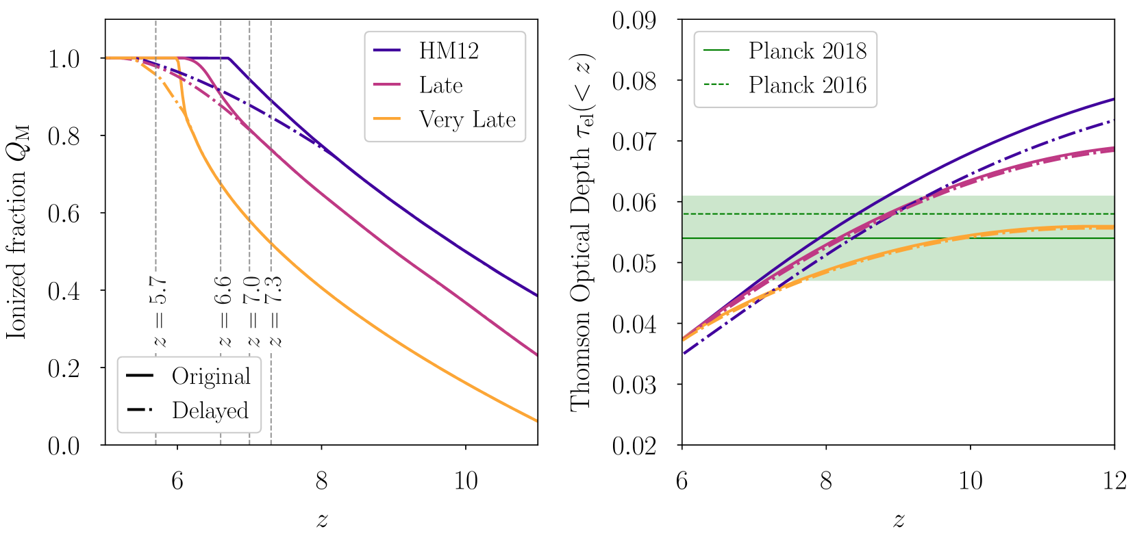
Figure 1: Left: Mass-averaged global ionized fraction for the reionization histories tested in this work, labelled HM12 (blue) Late (purple), Very Late (orange). The solid lines show the original models, whilst the dash-dotted lines are modified to have a delayed end to reionization. The HM12 model reionizes completely by $z=6.7$, whilst the Late/Very Late models finish by $z=6$, and the Delayed models finish at $z=5.3$. These six histories allow us to bracket the range of possible reionization paths that are constrained by CMB and Ly $\alpha$ forest measurements. Right: the Thomson optical depth to electron scattering as a function of redshift for the different reionization histories. For comparison the Planck Collaboration et al. (2018) and Planck Collaboration et al. (2016) CMB results are shown in green (with shading indicating the 1 $\sigma$ uncertainty).

LAEs have been established as a key tool for understanding the progress of reionization at $z\geq 6$. Given the resonant scattering of Ly $\alpha$ by neutral hydrogen in the intergalactic medium (IGM) and circumgalactic medium (CGM) (Gunn & Peterson, 1965; Madau & Rees, 2000), the visibility of LAEs should decrease as observations probe further into the reionization era (Dijkstra et al., 2007). This attenuation can be seen in the redshift evolution of both the luminosity function (e.g. Konno et al., 2018) and the clustering signal (e.g. Ouchi et al., 2018). Studies at lower redshifts are also important for understanding the ionizing photon budget, for example Nakajima et al. (2018) used LAEs to understand ionizing photon escape fractions, to determine if LAEs could have played a significant role in (re)ionizing their surrounding IGM. Green Pea galaxies, low-redshift analogs of LAEs, present a further avenue for understanding the properties of LAEs (Yang et al., 2016).

There has been extensive theoretical modelling of LAEs, considering both the ‘intrinsic’ Ly $\alpha$ emission properties of galaxies as a result of radiative transfer within the halo (such as Gronke & Dijkstra, 2016; Dijkstra, 2014; Zheng et al., 2010; Dijkstra & Westra, 2010; Laursen et al., 2009; Partridge & Peebles, 1967) as well as the effect of further attenuation by resonant scattering with neutral gas in the CGM and IGM (such as Laursen et al., 2018; Mason et al., 2018; Inoue et al., 2018; Weinberger et al., 2018; Sadoun et al., 2017; Kakiichi et al., 2016; Hutter et al., 2015; Mesinger et al., 2015; Choudhury et al., 2015; Hutter et al., 2014; Jensen et al., 2014, 2013; Bolton & Haehnelt, 2013; Laursen et al., 2011; Dijkstra et al., 2011; Dayal et al., 2009). In particular these two regimes are often modelled differently: the escape of Ly $\alpha$ photons from within a galaxy is frequently treated using full radiative transfer post-processing of high resolution hydrodynamic simulations (e.g. Verhamme et al., 2006), whilst the scattering in the IGM can be well approximated using $e^{-\tau}$ models (e.g. Laursen et al., 2011). On top of this it is important to model how LAEs form part of the wider galaxy population; Dijkstra & Wyithe (2012) for example modelled LAEs as a subset of the Lyman break galaxy (LBG) population with a $M_{UV}$-dependent distribution of Ly $\alpha$ equivalent widths. Given a mapping between host halo mass and galaxy UV luminosity, it is possible to employ such a model to fit the UV and Ly $\alpha$ luminosity function evolution, whilst also being consistent with observed equivalent width distributions. There is however some degeneracy in the mapping from mass to $M_{UV}$, which can be broken by considering the spatial clustering of LAEs (Lee et al., 2009). It is possible to fit all these observational constraints if a duty cycle is employed (Trenti et al., 2010).

In Weinberger et al. (2018) we employed large, high-dynamic-range hydrodynamical simulations of the IGM in combination with a semi-analytic reionization model in order to calculate the transmission of Ly $\alpha$ from LAE host haloes. The effects of the CGM, self-shielded neutral gas, and host halo mass dependence on the transmission were explored. In this work we now extend those transmission models to include an empirically-constrained model for the population of LAEs. Our modelling updates previous work and employs large scale simulations of the IGM to test the effects of reionization at observable redshifts, and to predict the LAE luminosity function, angular correlation function and rest-frame equivalent width probability distribution simultaneously. The underlying simulations have been used to model the 21 cm signal during reionization (Kulkarni et al., 2016) as well as opacity fluctuations after reionization (Kulkarni et al., 2018), such that we will be able to perform like-for-like comparisons with these other reionization observables in future work. This allows us to make predictions for the evolution of the Ly $\alpha$ luminosity function and clustering signal, which we compare to available observational data.

This paper is structured as follows: in section 2 we outline how we model the LAE populations using a suite of cosmological hydrodynamic simulations, then in section 3 we present a comparison of the predictions of our models with current observed data. In section 4 we discuss the assumptions of our modelling, before concluding in section 5.

2 Methods

2.1 Numerical simulations of the IGM

In order to model the IGM gas properties we employ the high-dynamic-range Sherwood simulation suite of cosmological hydrodynamic simulations (Bolton et al., 2017), with the same set up as in Weinberger et al. (2018). We refer the reader to that work for full details of the simulation and reionization modelling, but we summarize the salient points below.

The IGM gas properties are derived from the cosmological hydrodynamical simulations, which were performed using the P-Gadget-3 SPH code, a modified version of the original Gadget branch (Springel, 2005; Springel et al., 2001). In this work we utilize a simulation box of side length $L=320$ cMpc/h and particle number $N=2\times 2048^{3}$, so as to be large enough to capture the clustering signal at large scales. Dark matter haloes were identified on-the-fly using a friends-of-friends algorithm. The cosmological parameters were set to match the Planck Collaboration et al. (2014) results: $h=0.678$, $\Omega_{m}=0.308$, $\Omega_{\Lambda}=0.692$, $\Omega_{b}=0.0482$, $\sigma_{8}=0.829$, $n=0.961$, and $Y_{\mathrm{He}}=0.24$. The gas properties were smoothed onto a uniform grid with cell size $L_{\mathrm{cell}}=156.25$ ckpc/h, using the SPH kernel.

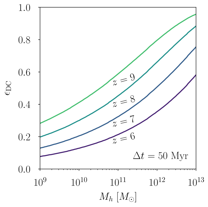
Figure 2: Effective duty cycle defined by Trenti et al. (2010), as a function of halo mass and redshift, where $\Delta t$ is a free parameter. This weights the abundance matching towards haloes that could have formed within $\Delta t$; for example shown here is our fiducial choice of $\Delta t=50$ Myr.

In order to derive the ionization properties of the gas, a semi-analytic framework is employed in which the large-scale ionization is modelled using an excursion set approach (Furlanetto et al., 2004; Mesinger & Furlanetto, 2007; Choudhury et al., 2009; Mesinger et al., 2011; Santos et al., 2010; Hassan et al., 2016) whilst the small-scale ionization is calibrated self-consistently within the simulation volume (Choudhury et al., 2015; Kulkarni et al., 2016). In particular we use the self-shielding prescription of Chardin et al. (2018), itself a modification of the Rahmati et al. (2013) parametrization, in order to accurately model small-scale neutral features. This framework allows us to test arbitrary reionization histories without needing to explicitly model the ionizing emissivity of sources. In appendix A we compare this excursion set scheme to a full radiative transfer calculation, and find that our results are largely insensitive to the use of this approximation.

As in Weinberger et al. (2018), we will test the three bracketing reionization histories first established in Choudhury et al. (2015), referred to as HM12, Late and Very Late. The evolution of the mass-averaged global neutral fraction in these models can be seen in the left panel of Figure 1 with the solid lines. We note that in the early HM12 model, reionization ends (i.e. when $Q(z_{\mathrm{end}})=1$) at $z=6.7$. The Late model is the same as the HM12 model but shifted in redshift so that reionization is completed by $z=6$. Finally in the Very Late model reionization also ends at $z=6$ but with a different redshift gradient $\mathrm{d}Q/\mathrm{d}z$, so that it finishes more abruptly. In this work we also consider modified versions of these three models in which the end of reionization is delayed to $z\sim 5.3$, but with the same evolution at higher redshifts. These will be referred to as the “Delayed” models (in comparison to the “Original” models). Physically these delayed models can result from an ionizing emissivity evolution that peaks around $z\sim 7$ and then falls dramatically at lower redshifts, as suggested in Puchwein et al. (2018). We note that the Delayed Very Late reionization history has a similar neutral fraction evolution to the model of Kulkarni et al. (2018), which was found to reproduce the opacity fluctuations in the Lyman-$\alpha$ forest (after reionization). The Delayed models are shown in Figure 1 with the dash-dotted lines. In the right panel of Figure 1 we compare the electron scattering optical depths predicted by these histories with the recent Planck CMB measurements. The low value of $\tau=0.054\pm 0.007$ measured by Planck Collaboration et al. (2018) favours a later reionization, and we see that our Very Late models are consistent within 1$\sigma$ of this recent measurement.

These reionization histories are then calibrated on the simulation so that the background photoionization rate, $\Gamma_{\mathrm{HI}}$, (which is naturally coupled to the global average ionization fraction) is self-consistent. The strength of the self-shielding and the equilibrium value of the neutral fraction within ionized regions is dependent on this UV background. Our calibrated simulation is also consistent with observed background photoionization rates and ionizing photon mean free paths (Faucher-Giguère et al., 2009; Calverley et al., 2011; Wyithe & Bolton, 2011) and the observed CMB optical depth Planck Collaboration et al. (2018). We note that our Very Late models are also consistent with current observational estimates from the SILVERRUSH survey on the neutral fraction evolution (see appendix C).

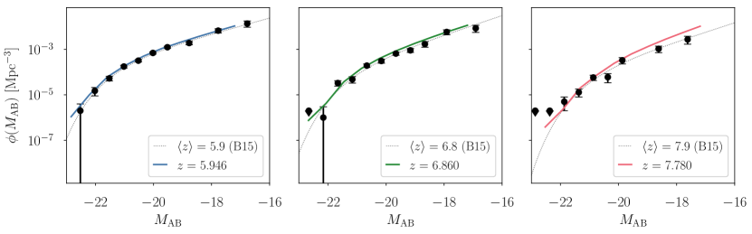
Figure 3: The evolution of the LBG UV luminosity function. The thick solid lines show our model predictions, compared to the data-points from Bouwens et al. (2015) (and the dotted line best fit Schechter functions). The abundance matching is performed at $z=5.9$, so the agreement in the left-most panel is by construction. At higher redshift the evolution is due to the evolution of the halo mass function, and we see good agreement between our model predictions and the observed luminosity functions.

2.2 Populating haloes with LBGs

We implement the Improved Conditional Luminosity Function (ICLF) method of Trenti et al. (2010) in order to populate the dark matter haloes in our simulations with LBG-type galaxies. This involves abundance matching the halo mass function to the observed UV luminosity function (as in, e.g. Lee et al., 2009; Bouwens et al., 2008). This assumes that each halo hosts one galaxy, and then equates the number of halos above a certian mass $M_{h}$ with the number of LBGs above a certain luminosity $L_{\mathrm{UV}}$,

$$\epsilon_{\mathrm{DC}}(M_{h},z)\int_{M_{h}}^{\infty}n(M,z)\mathrm{d}M=\int_{L_{\mathrm{UV}}}^{\infty}\phi(L,z)\mathrm{d}L,$$ (1)

where $n(M,z)$ is the halo mass function, $\phi(L,z)$ is the UV luminosity function, and $\epsilon_{\mathrm{DC}}(M_{h},z)\leq 1$ is a mass and redshift dependent duty cycle which accounts for how likely it is that we will observe the galaxy hosted by a given halo at a particular time. Eq. (1) implicitly defines a mapping between halo mass and UV luminosity, $L_{\mathrm{UV}}(M_{h})$. We use the same form of the duty cycle as Trenti et al. (2010),

$$\epsilon_{\mathrm{DC}}(M_{h},z)=\frac{\int_{M_{h}}^{\infty}\mathrm{d}M\left[n(M,z)-n(M,z_{\Delta t})\right]}{\int_{M_{h}}^{\infty}\mathrm{d}M\>n(M,z)}.$$ (2)

Note that,

$$\Delta t=t_{H}(z)-t_{H}(z_{\Delta t}),$$ (3)

where $t_{H}$ is the local Hubble time (Trenti & Stiavelli, 2009). $\Delta t$ is a free parameter in this duty cycle model; in this work we choose $\Delta t=50$ Myr (originally a duty cycle with $\Delta t=200$ Myr was employed by Trenti et al., 2010). The time interval between $z=10$ and $z=6$ (when reionization is underway) is less than 500 Myr, and so we choose a smaller $\Delta t$ to reflect the bursty nature of star formation across this period. We note that other numerical work has found similar time scales for luminosity variation between 10–100 Myr, such as Rosdahl et al. (2018) who found large temporal variation of the fraction of escaping ionizing photons, $f_{\mathrm{esc}}$, from galaxies during reionization. Our choice will be further justified when we present the effect that varying $\Delta t$ has on the clustering signal in section 4.1. The $\Delta t=50$ Myr duty cycle as a function of redshift and mass is shown in Figure 2. We finally note that the $\Delta t$ parameter itself may in reality evolve with cosmic time, which would affect the evolution of the clustering signal of galaxies.

A heuristic picture of this duty cycle is as follows: although we expect galaxies to exist in most dark matter haloes (above a minimum mass), it is not the case that we expect these galaxies to always be bright enough (in the UV) to be observed. The stochastic nature of star formation, and possibly geometric radiative transfer effects, might allow us to only observe a fraction of the underlying galaxy population (at a given time). In the above abundance matching procedure, enforcing a duty cycle will alter the mapping $L_{\mathrm{UV}}(M_{h})$ in such a way as to shift the mapping to lower masses. This means lower mass haloes can be brighter (compared to the result if $\epsilon_{\mathrm{DC}}=1$), which will further impact the clustering. Recently, Gurung López et al. (2018) explored the role of radiative transfer effects within a given Ly $\alpha$ emitting galaxy, and found that carefully including these effects for a population of LAEs causes the LAEs to reside in less massive host haloes (compared to when such RT effects are neglected). Although our duty cycle is somewhat more agnostic to specific internal galaxy physics, it has the same effect. As in that work, we find that populating less massive haloes leads to better agreement with observables such as the clustering signal (Lee et al., 2009).

We perform the abundance matching detailed in Eq. (1) using the Sheth-Mo-Tormen (SMT) halo mass function (Sheth et al., 2001), with HMFcalc (Murray et al., 2013). For the UV luminosity functions, we employ the best-fit Schechter functions from Bouwens et al. (2015). In particular we calibrate our luminosity mapping $L_{\mathrm{UV}}(M_{h})$ at $\langle z\rangle=5.9$, and can then apply this to the halo populations at each redshift of interest. Trenti et al. (2010) found that their mapping, calibrated at $z\sim 6$, was able to capture the evolution down to $z\sim 4$ of the observed UV luminosity function. The shape of $L_{\mathrm{UV}}(M_{h})$ we find is similar to that found by Trenti et al. (2010), but shifted to lower masses due to the lower $\Delta t$ that we employ in this work.

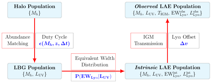
Figure 4: Summary schematic representing the different parts of the LAE modelling: first the halo population of a given simulation snapshot is abundance matched to the observed UV population with an assumed duty cycle, to create a mock LBG population. Then we draw from an empirical ‘intrinsic’ REW distribution to create a mock ‘intrinsic’ LAE population. Finally the effects of IGM transmission are taken into account to create a mock ‘observed’ LAE population.

We can test that the evolution of the UV luminosity function is well fit by the underlying halo mass evolution by using the $L_{\mathrm{UV}}(M_{h})$ mapping on the simulated halo populations. In Figure 3 we show this evolution starting with the calibrated redshift $z=5.9$ on the left, and then higher redshifts on the right. Note the average redshift of the observational sample can be compared to the precise redshift of the simulation snapshot in the lower righthand subplot legends.

After this step in the framework, we now have an observationally calibrated mock sample of LBGs in our simulation. A subset of these will end up as a final LAE mock sample, after the selection detailed below.

2.3 LAE equivalent width distribution

We implement the rest-frame equivalent width (REW) distribution model proposed by Dijkstra & Wyithe (2012) in order to determine which of our LBG population will have observable Ly $\alpha$ emission. This is calibrated to empirical equivalent width distributions, therefore bypassing the need to model Ly $\alpha$ escape fractions and emission mechanisms. The model starts with a $M_{\mathrm{UV}}$-dependent distribution of Ly $\alpha$ REWs,

$$P(\mathrm{REW}|M_{\mathrm{UV}})=\mathcal{N}\exp{\left(-\frac{\mathrm{REW}}{\mathrm{REW}_{c}(M_{\mathrm{UV}})}\right)},$$ (4)

where $\mathrm{REW}_{c}(M_{\mathrm{UV}})$ is a charactestic REW for a given $M_{\mathrm{UV}}$, given by (the best fit model of Dijkstra & Wyithe, 2012),

$$\mathrm{REW}_{c}(M_{\mathrm{UV}})=23+7(M_{\mathrm{UV}}+21.9)+6(z-4).$$ (5)

The normalization is defined such that the population has $\mathrm{REW}_{\mathrm{min}}\leq\mathrm{REW}\leq\mathrm{REW}_{\mathrm{max}}$, where we choose $\mathrm{REW}_{\mathrm{max}}=300$ Å, and $\mathrm{REW}_{\mathrm{min}}$ is a function of $M_{\mathrm{UV}}$,

$$\mathrm{REW}_{\mathrm{min}}=\\ \begin{cases}-20\text{ \AA}&\quad M_{\mathrm{UV}}<-21.5;\\ 17.5\text{ \AA}&\quad M_{\mathrm{UV}}>-19.0;\\ -20+6(M_{\mathrm{UV}}+21.5)^{2}\text{ \AA}&\quad\mathrm{otherwise}.\end{cases}$$ (6)

Therefore the explicit form for the ($M_{\mathrm{UV}}$-dependent) normalization is,

$$\mathcal{N}=\frac{1}{\mathrm{REW}_{c}}\left(\exp{\left(\frac{-\mathrm{REW}_{\mathrm{min}}}{\mathrm{REW}_{c}}\right)}-\exp{\left(\frac{-\mathrm{REW}_{\mathrm{max}}}{\mathrm{REW}_{c}}\right)}\right)^{-1}$$ (7)

This choice of $M_{\mathrm{UV}}$ dependence reproduces the so-called Ando relation (Ando et al., 2007). We note Dijkstra & Wyithe (2012) compared this choice of distribution to the observed distributions at $z=$ 3.1, 3.7 and 5.7 by Ouchi et al. (2008). They found good agreement at the lower redshifts, but that their model over-estimated the number of large REW systems at the higher redshifts. This was calculated in the absence of attenuation by the CGM/IGM, which is non-zero even after reionization has completed at $z\sim 6$. We find that the inclusion of an IGM transmission fraction $<1$ compensates for the overprediction, and hence we do not modify the model to try to correct this. We further discuss this in section 3.3.

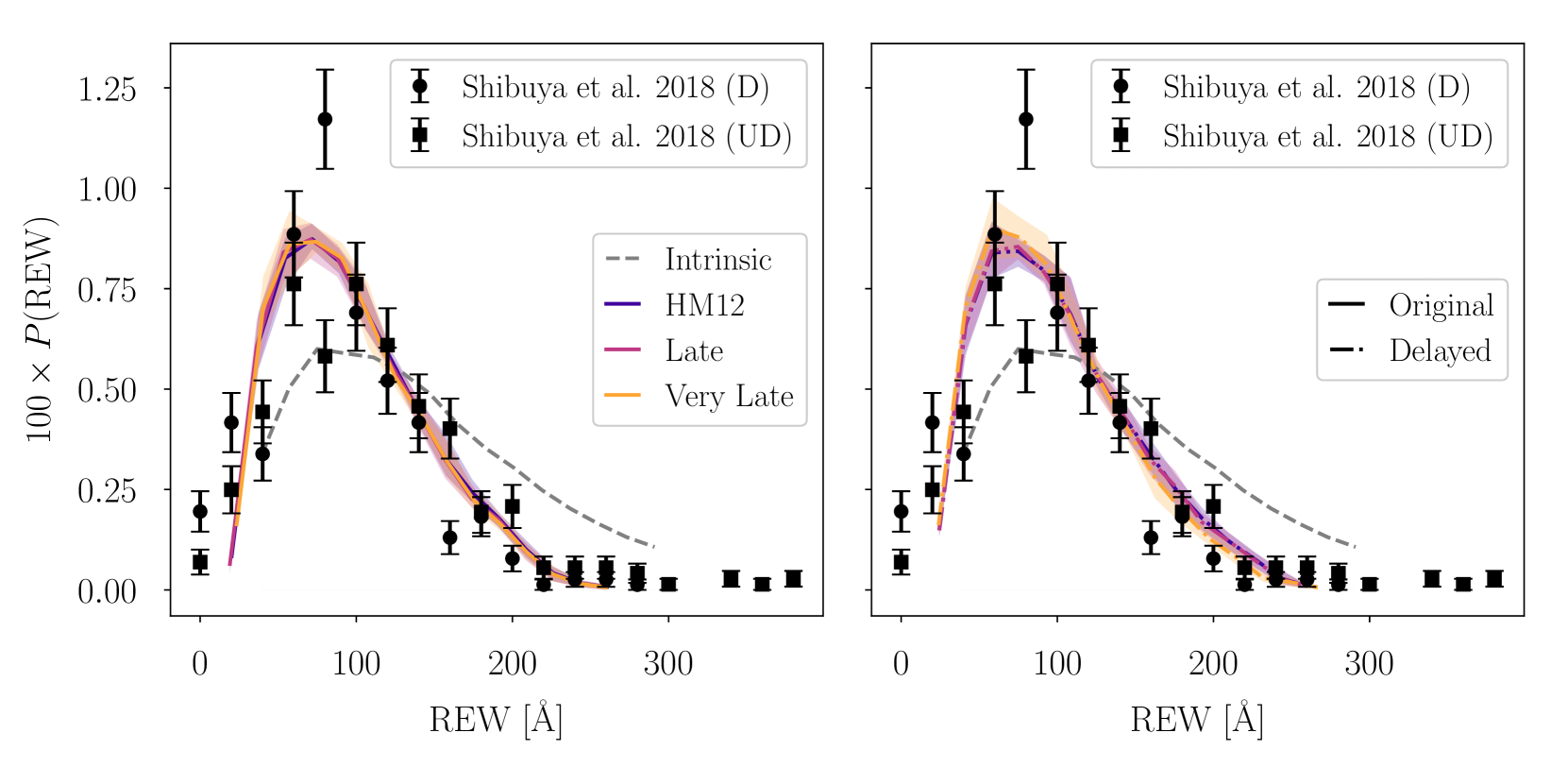
Figure 5: Comparison of our model mock REW distribution at $z=5.756$ with the observed distribution from the SILVERRUSH survey at $z=5.7$. The different reionization histories are shown by the different colours, whilst the intrinsic un-attenuated model is shown with the grey dashed line. On the left hand panel in the solid lines we show the original reionization histories; on the right hand panel we show the Delayed models with dash-dotted lines. For the chosen emission offset parameter, $\Delta v\propto v_{\mathrm{circ}}$, we find that the IGM transmission corrects the over-abundance of high REW systems predicted by the intrinsic model.

For each of the haloes in our LBG sample, we draw a random REW from this conditional probability distribution, thereby assigning them a Ly $\alpha$ luminosity defined by,

$$L_{\mathrm{Ly\alpha}}=\frac{\nu_{\alpha}}{\lambda_{\alpha}}\left(\frac{\lambda_{\mathrm{UV}}}{\lambda_{\alpha}}\right)^{-\beta-2}\times\mathrm{REW}\times L_{\mathrm{UV,\nu}},$$ (8)

where $\nu_{\alpha}=2.47\times 10^{15}$ Hz is the Ly $\alpha$ transition frequency, $\lambda_{\alpha}=1216$ Å the corresponding Ly $\alpha$ wavelength, $\lambda_{\mathrm{UV}}=1600$ Å is the rest-frame wavelength at which the UV luminosity function was measured (Bouwens et al., 2015), $\beta=-1.7$ is the assumed UV spectral index, and the UV luminosity density, $L_{\mathrm{UV,\nu}}$, is related to $M_{\mathrm{UV}}$ by (Ouchi et al., 2008),

$$M_{\mathrm{UV}}=-2.5\log{L_{\mathrm{UV,\nu}}}+51.6.$$ (9)

Having generated $L_{\mathrm{Ly\alpha}}$ for the LBG mock sample, we then apply selections based on luminosity and equivalent width limits to match a given observational study. Table (1) shows some of the observational thresholds used in the SILVERRUSH survey (Ouchi et al., 2018; Konno et al., 2018; Shibuya et al., 2018), which we adopt here.

Table 1: Observational selection thresholds^† used in this work to generate mock observed samples.

Based on survey	$z$	REWmin [Å]	$L_{\mathrm{Ly\alpha,min}}^{\dagger\dagger}$ [erg/s]
Konno et al. (2018)	5.7	10	6.3$\times 10^{42}$
Konno et al. (2018)	6.6	14	7.9$\times 10^{42}$
Ota et al. (2017)	7.0	10	2$\times 10^{42}$
Itoh et al. (2018)
Konno et al. (2014)	7.3	0	2.4$\times 10^{42}$

Note:

^†The observational surveys we derived these limits from measured different fields on the sky, across which different selection thresholds were sometimes applied. The values we have chosen are representative despite this variation.

^††As in Dijkstra & Wyithe (2012), when not quoted in the original survey, we estimate $L_{\mathrm{min}}$ as the lower bin edge of the lowest luminosity bin in the presented luminosity function.

We note that Dijkstra & Wyithe (2012) concluded that equivalent width and luminosity cuts are only an approximation to the real selection thresholds used in observational LAE studies. They found that in order to match both the observed equivalent width distribution and the luminosity function, they had to scale the number density by $\sim 0.5$. With this scaling included, their modelling then matched the redshift evolution very well.

When calculating the IGM transmission (as described in detail in section  2.4) in our simulations we find that even at $z=5.7$ the transmission redwards of Ly $\alpha$ is not 100%. As was suggested in Sadoun et al. (2017) (and explored further in Weinberger et al., 2018), this is due mostly to the neutral gas in the outer part of the host halo (close to the virial radius), controlled by the background photoionization rate (see section 3.2). In our delayed models there is also an increased fraction of neutral gas in the rest of the IGM, but we find the attenuation at these redshifts is dominated by CGM and surrounding halo gas . This means that when we include the transmission we find the number density of ‘observed’ LAEs drops, in good agreement with the real observed luminosity functions. We therefore choose to use the REW distribution from Dijkstra & Wyithe (2012) to model the ‘intrinsinc’ distribution of our population, which is then attenuated by the IGM to give the ‘observed’ REWs and Ly $\alpha$ luminosities. As such we do not apply the $\sim 0.5$ scaling to the number density in our model predictions which was needed in Dijkstra & Wyithe (2012); we find agreement with the observational results without this.

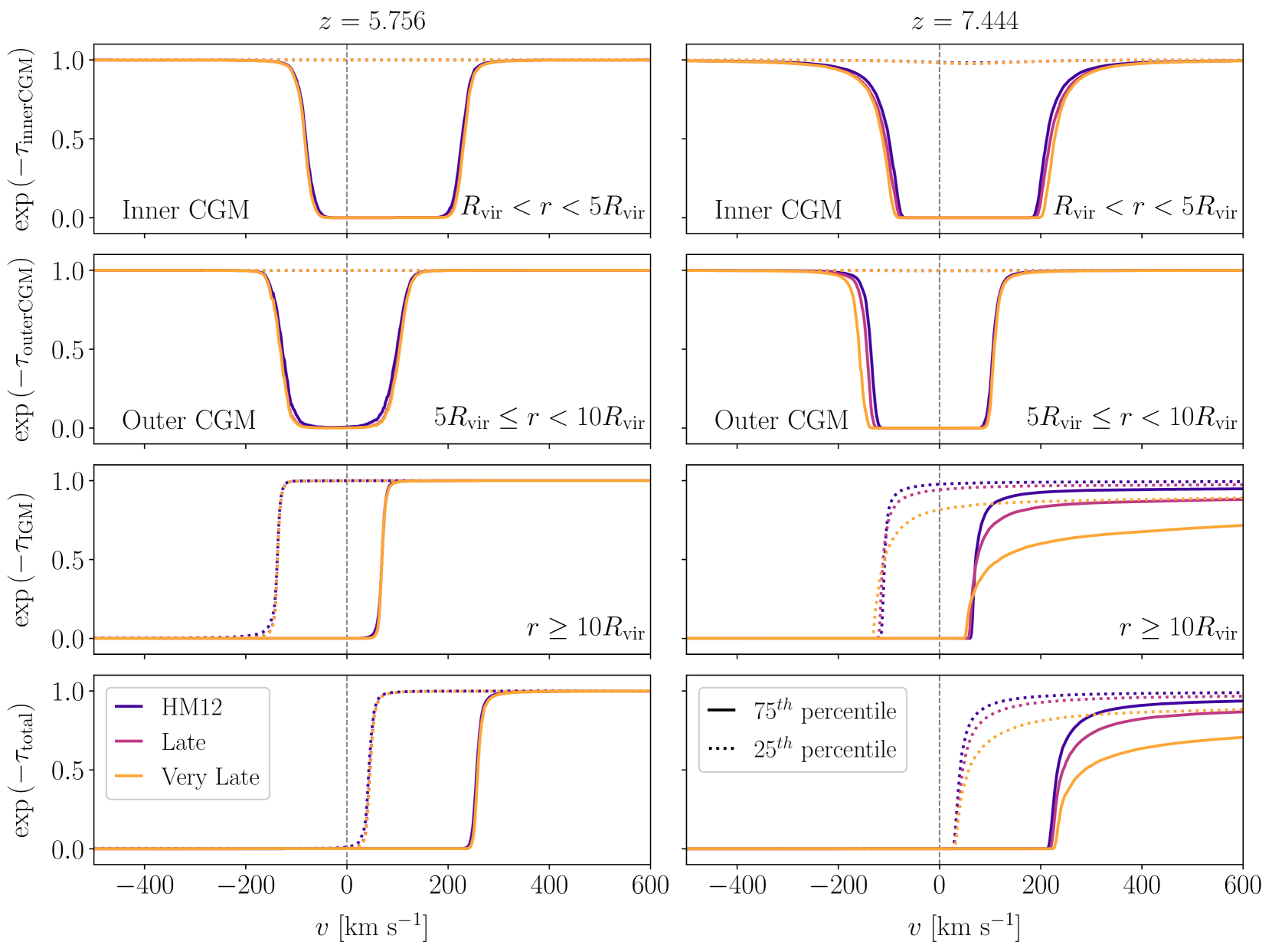
Figure 6: Separating the contributions to the Ly $\alpha$ transmission: (i) in the top panels we show the transmission due to the CGM and surrounding gas (split into an “inner” part between $R_{\mathrm{vir}}<r<5R_{\mathrm{vir}}$ and an “outer” part between $5R_{\mathrm{vir}}\leq r<10R_{\mathrm{vir}}$) (ii) in the middle panels the contribution from the IGM ($r\geq 10R_{\mathrm{vir}}$); (iii) in the bottom panels the transmission from all the gas outside the halo ($r>R_{\mathrm{vir}}$). In all panels the solid (dotted) curves correpond to the $75^{th}$ ($25^{th}$) percentile as measured across our mock observed sample of LAEs (i.e. after $L_{\mathrm{Ly\alpha}}$ and REW selection), which spans an order of magnitude in luminosity. The transmission is shown as a function of velocity offset from line-centre, at redshift $z=5.756$ on the left and $z=7.444$ on the right. The three original reionization histories are shown using the coloured solid lines. For clarity we do not plot the delayed-end models, however their corresponding transmission curves are very similar.

This means we now have a mock LAE sample, in which each object has a value of $M_{h}$, $M_{\mathrm{UV}}$, REW, and $L_{\mathrm{Ly\alpha}}$ that conforms to the chosen observational selection window. The final step in the framework, before we can compare with observations, is to calculate the IGM transmission fraction for a given halo in the sample, and reduce the luminosity accordingly.

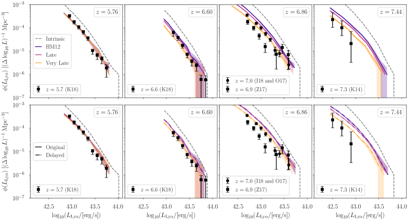
Figure 7: From left to right: The luminosity function evolution, at $z=5.756$, 6.604, 6.860 and 7.444, for each of the reionization histories shown as coloured lines. The top panel with solid lines shows the original three reionization histories, whilst the bottom panel with dash-dotted lines shows the delayed-end histories. Some observed data is overplotted for comparison with black markers, from Konno et al. (2018) (K18, $z=5.7$ & 6.6), Itoh et al. (2018) (I18, $z=7.0$), Ota et al. (2017) (O17, $z=7.0$), Zheng et al. (2017) (Z17, $z=6.9$), Konno et al. (2014) (K14, $z=7.3$).

2.4 Ly $\alpha$ transmission

We calculate the CGM/IGM transmission as in Weinberger et al. (2018), extracting sightlines through the halo sample to find the optical depth to Ly $\alpha$, $\tau_{\mathrm{Ly\alpha}}(v)$, as a function of velocity offset from the emitter (Bolton & Haehnelt, 2007). This can be used to calculate a transmission fraction, assuming an intrinsic emission profile $J(v)$ for the galaxy, which itself accounts for the radiative transfer within the halo as photons escape the galaxy’s ISM. The emission profiles of LAEs seen in both observations (e.g. Hashimoto et al., 2015) and radiative transfer simulations (e.g. Zheng & Wallace, 2014) are non-trivial to model, with complicated dependences on the local gas dynamics.

We make the simplifying assumption that the emission profile is a single-peaked Gaussian profile with width $\sigma_{v}$, offset redwards from the systemic by $\Delta v$ due to resonant scattering within the halo. We choose $\sigma_{v}=88$ km/s as in Choudhury et al. (2015). Our fiducial choice for the velocity offset is to set it proportional to the virial circular velocity of a given LAE’s host halo, $\Delta v\propto v_{\mathrm{circ}}$. This is motivated by observational and theoretical work such as Verhamme et al. (2018); Smith et al. (2018); Dijkstra et al. (2006); Neufeld (1990), which has shown that the radiative transfer (as a strong function of HI opacity) in a galaxy’s ISM/CGM leads to a coupling between the dispersion of the Ly $\alpha$ line and its velocity offset. We might expect the dispersion to be proportional to a halo’s circular velocity, which in turn gives the same proportionality for the offset. Previously in Weinberger et al. (2018) we used a fixed value of $\Delta v=100$ km/s, neglecting any dependence on the emitter properties and assuming no variation across the population. Although this choice was simplistic, we found that the relative transmission fraction, $T^{\mathrm{IGM}}_{\mathrm{Ly\alpha}}(z)/T^{\mathrm{IGM}}_{\mathrm{Ly\alpha}}(z=5.7)$, was largely insensitive to this choice. In the present work we now need to consider the absolute transmission fraction at a given redshift and so we have updated our model for the intrinsic emission.

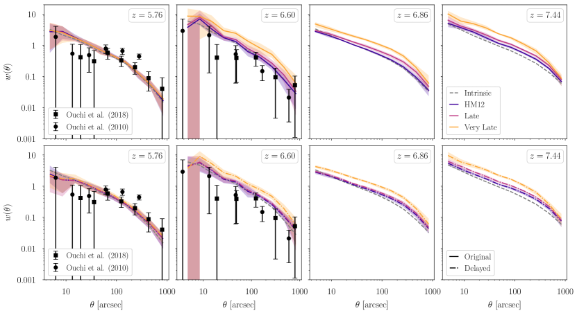
Figure 8: From left to right: The angular correlation function, measuring the clustering signal at $z=5.756$, 6.604, 6.860 and 7.444, for our fiducial model with $\Delta t=50$ Myr. As in Figure 6, the top panel shows the original reionization histories in solid lines, whilst the bottom panel shows the delayed-end versions in dash-dotted lines. At $z=5.756$ the reionization histories have converged (reionization has ended) and so the models are equivalent. At higher redshifts we start to see some divergence of the amount of clustering predicted for each reionization history, with the Very Late model predicting the most clustering power. For each redshift these mock surveys correspond to 10 slices of our simulation volume (each with area $320\times 320$ (cMpc/h)²), therefore simulating a total survey area of $2.2$ Gpc². We also refer the reader to Table (1) for the mock selection limits used at each redshift.

Other theoretical works have treated the intrinsic emission profile differently, for example Inoue et al. (2018) used the single peaked profiles that result from full radiative transfer calculations applied to an outflowing spherical volume of gas. This is strongly dependent on the chosen HI column density and outflow velocity; our modelling assumes an explicit halo mass dependence for the profile rather than fixing these quantities across the population.

We finally note that this is a poorly constrained quantity observationally, and so we later test the effect of varying our $\Delta v$ assumption. In reality the intrinsic emission profile of an LAE will evolve and vary across its lifetime, a feature we do not attempt to model in this work.

The transmission fraction for this profile can then calculated as (Mesinger et al., 2015),

$$T^{\mathrm{IGM}}_{\mathrm{Ly\alpha}}=\frac{\int\mathrm{d}\nu\>J(\nu)\>e^{-\tau(\nu)}}{\int\mathrm{d}\nu\>J(\nu)}.$$ (10)

Note that specifically this is the transmission fraction redwards of systemic; in choosing a single-peaked profile we have accepted that the IGM is sufficiently optically thick at the redshifts we consider such that even if a blue peak emerges after radiative transfer in the ISM, the HI damping wing of the IGM will not transmit bluewards of systemic. This method of separating the radiative transfer into a galaxy stage (which we simply model with our velocity offset $\Delta v$) and an IGM stage (which we model using the $e^{-\tau}$ approximation) has been employed successfully before, for example in Laursen et al. (2018, 2011). As we account for the galactic radiative transfer already, we exclude the host halo gas in our calculation of $\tau_{\mathrm{Ly\alpha}}$. Our fiducial choice is to exclude halo gas within 1 $R_{\mathrm{vir}}$ of the halo centre, the effect of which was tested in Weinberger et al. (2018). Similarly Laursen et al. (2018) chose to transition between the two calculation regimes at 1.5 $R_{\mathrm{vir}}$. We reiterate that the choice of intrinsic emission profile has a strong effect on the transmission fraction, and therefore also on the resulting population statistics for our LAE mock catalogues.

Having performed the transmission fraction calculation for each halo, we can update the derived Ly $\alpha$ luminosity,

$$L^{\mathrm{obs}}_{\mathrm{Ly\alpha}}=T^{\mathrm{IGM}}_{\mathrm{Ly\alpha}}L_{\mathrm{Ly\alpha}},$$ (11)

and similarly for the equivalent widths. This completes our generation of a mock LAE sample from our simulated halo population. This framework allows us to generate samples at any desired redshift to compare with observations, and make predictions at higher redshifts for the evolution of the luminosity function and clustering signal. Note that when the transmission fraction falls below unity, some of the LAEs will drop below the flux-limit, hence we reapply the selection after accounting for transmission. In Figure 4 we show a summary schematic for the different stages of the LAE modelling.

2.5 Modelling caveats

Although this model framework is successful at matching the evolution of observed luminosity functions and clustering studies (as we will present in section 3), there are a number of important caveats to consider:

• We do not use sub-find catalogs with satellite haloes. As we are only using central haloes we will naturally underestimate the 1-halo term of the clustering signal. However at the redshifts of interest $z\gtrsim 6$ the halo occupation distribution (HOD) populates only very large mass haloes with satellites. For example Bhowmick et al. (2018) found that the satellite fraction of haloes is around $\sim 10\%$ at $z=7.5$, and that the mean number of satellites is less than unity for halo masses below $M_{h}\sim 10^{11}\>M_{\odot}/h$. Similarly Gurung López et al. (2018) found that satellite galaxies only start to dominate the abundance of haloes with mass $M_{h}\gtrsim 10^{12}\>M_{\odot}/h$.

• There are a number of tunable parameters in this model. The primary free parameters are $\Delta t$ which controls the duty cycle, and $\Delta v$ which controls the ‘intrinsic’ emission profile and hence has a strong effect on the calculated transmission fraction. We take the best-fit REW distribution from Dijkstra & Wyithe (2012) and so do not leave any of those model parameters free, but use their empirically constrained values.

• Although we predict the transmission, and leave the duty cycle as a free parameter, these variables have a degenerate effect on the clustering. Increasing (decreasing) the duty cycle (the transmission) can lead to an increase in the measured clustering signal. We have used physically motivated values for the free parameters $\Delta t$ and $\Delta v$.

3 Results

We now discuss the results of applying our LAE framework to the halo population in the Sherwood simulations. In particular we consider the IGM transmission across this population, and how this affects the luminosity function evolution. We also confirm that our model matches the observed equivalent width distribution and luminosity function at $z=5.7$. Taking this redshift as an anchor we then also create mock survey slices from which we calculate the angular correlation function, a 2-point measure of the clustering signal. Finally we extend our models to higher redshifts to make predictions for future surveys.

Note for all plots where we compare our model predictions to the observational data, we have taken slices of the simulation volume and calculated the relevant statistical quantity for the sample of LAEs in each slice. The shading shown for the model predictions corresponds to 68% scatter across the slices. Specifically we divide the box up in configuration-space into 10 slices perpendicular to the direction along which we calculated the transmission, giving a comoving thickness of 32 cMpc/h. This is not exactly equivalent to the narrowband selection, which is instead a slice in redshift (velocity) space; however given the width of the narrowband slice and the comparatively small amplitudes of peculiar motions of the LAEs in our simulation volume, we find that the results using configuration-space slicing are indistinguishable from the velocity-space slicing. In all figures we show the intrinsic (unattenuated) quantities using a dashed grey line, whilst the different model (attenuated) quantities are shown using coloured solid lines (original reionization histories) and dash-dotted lines (delayed-end models).

3.1 IGM attenuation of the $z=5.7$ equivalent width distribution

In Figure 5 we compare the observed REW distribution from the SILVERRUSH survey (Shibuya et al., 2018) at $z=5.7$ with that predicted from our mock LAE population. We show the un-attenuated ‘intrinsic’ distribution with the dashed grey line, whilst the IGM attenuated distributions are shown for the three different reionization histories in blue (HM12), purple (Late) and orange (Very Late).

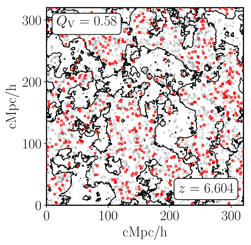
Figure 9: A mock map of a sample of LAEs within a 32 cMpc/h slice of the simulation volume, showing the whole population in grey empty circles and those above the observational thresholds in red empty squares. A black contour at a value of half the maximum projected neutral fraction is also plotted, segregating the regions within this projected slice which are largely neutral from those which are ionized. It is visible by eye that the majority of the observed mock LAEs (in red) lie within the ionized regions.

We see at this redshift that although our original reionization histories give a global average ionized fraction of unity, the IGM transmission fraction is sufficiently below unity that it has a significant effect on the observed REW distribution. This attenuation results from (photoionization) equilibrium and self-shielded neutral gas around haloes which contributes little to the average ionized fraction but has a strong effect on the Ly $\alpha$ attenuation (see section  3.2). In particular the transmission fraction distribution is such that it attenuates the high REW objects, thereby reducing the over-abundance of such objects which is predicted by the intrinsic distribution. We have chosen to use a velocity offset of $\Delta v=a\>v_{\mathrm{circ}}$ where,

$$a=\begin{cases}1.5&\mathrm{Original},\\ 1.8&\mathrm{Delayed},\end{cases}$$ (12)

which gives a distribution consistent with the observed data. We also tested proportionality constants $a=1$ and $a=2$ and found that these resulted in either too much attenuation or too little, respectively. The larger value of $a$ is required in the Delayed models, where reionization has not yet ended by $z=5.7$, so there is considerably more attenuation by residual neutral gas. In particular we find that these models require a lower background photoionization rate, therefore increasing the amount of neutral gas present in the outer parts of the LAE host haloes (in the CGM). The presence of this gas is sufficient to reduce the transmission redwards of Ly $\alpha$.

The resonant scattering of Ly $\alpha$ radiation by neutral hydrogen within the galaxy tends to diffuse the emission profile away from line-centre, with radiation escaping in blue or red peaks where the scattering cross-section is smaller. If the galaxy has outflows, the red peak can be enhanced such that the dominant emission comes at redder velocities. This is seen in shell models with an expanding H i outflow (e.g. Dijkstra et al., 2011; Verhamme et al., 2006). We might therefore expect that the velocity offset $\Delta v$ should be coupled to the galaxy wind velocity which, to avoid stalling, must be of order the escape velocity of the halo, i.e. $\sim\sqrt{2}v_{\mathrm{circ}}$. Hence the values of $a$ in Eq. (12) are reasonable.

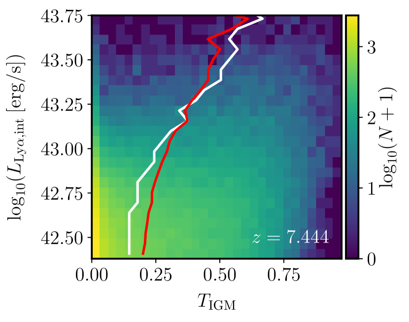
Figure 10: Histogram for the transmission fraction distribution and the ‘intrinsic’ Ly $\alpha$ luminosity for our mock LAE population at $z=7.444$. The number of objects in each bin is indicated by the colourmap, whilst the red (white) line indicates the mean (median) transmission fraction for a given luminosity bin. We see that the brighter LAEs are preferentially more visible than the fainter LAEs.

3.2 Attenuation from the partially neutral CGM

As seen in section 3.1, even at $z=5.756$ (where our original reionization histories are fully reionized, i.e. $Q_{\mathrm{M}}=1$) there is still an attenuation of radiation redwards of Ly $\alpha$. This is due to infalling neutral gas around the halo (including the CGM around the LAEs), which is not fully ionized by either the LAE itself or the ionizing UV background. Sadoun et al. (2017) found that the drop in observed numbers of LAEs doesn’t necessarily imply a largely neutral IGM, since this infalling CGM gas can also bring the Ly $\alpha$ transmission below $100\%$. We note again that our usage of the term CGM refers to a larger volume of the infalling gas that surrounds the host halo than the more common observational definition.

To quantify this further, in Figure 6 we plot the $75^{th}$ and $25^{th}$ percentiles of the transmission along sightlines to our observed samples of mock LAEs. We show the transmission as a function of velocity offset from line-centre due to: (i) the infalling CGM and surrounding gas (split into an “inner” part between $R_{\mathrm{vir}}<r<5R_{\mathrm{vir}}$ and an “outer” part between $5R_{\mathrm{vir}}\leq r<10R_{\mathrm{vir}}$ around the halo center); (ii) the exterior IGM gas ($r\geq 10R_{\mathrm{vir}}$); and (iii) the total gas around the LAE. We show this for our three original reionization histories at the two bracketing redshifts. We see that there is significant halo-to-halo variation in the CGM component, where the transmission can vary from 100% at all velocities (in the $25^{th}$ percentile) to 0% around $v=0$ km/s (in the $75^{th}$ percentile). In the left panel (at $z=5.756$) we see that the IGM is transmitting at $\sim 100\%$ redwards of Ly $\alpha$ (i.e. $v>0$ km/s) for the $25^{th}$ percentile, whereas the $75^{th}$ percentile starts to transmit at $\sim 100\%$ for redder velocities $v\gtrsim 100$ km/s. Furthermore we see the drop in transmission due to the CGM gas extends redwards of line-centre, because the gas is infalling onto the halo. In particular the “inner” part of the CGM attenuates redwards of the “outer” part because the amplitude of the infalling gas velocity peaks in that region. This means that radiation redwards of line-centre can be blue-shifted in the frame of the gas towards line-centre, and hence resonantly scattered out of the line of sight. The CGM transmission evolves across the redshifts as a function of the photoionization rate, which controls how neutral the gas is.

Figure 11: Histogram for the mass distribution and the ‘observed’ Ly $\alpha$ luminosity for our mock LAE population at $z=5.756$. The number of objects in each bin is indicated by the colourmap, whilst the red (white) line indicates the mean (median) host halo mass for a given luminosity bin. The white datapoint shows the median luminosity and effective halo mass for the NB816 sample of Khostovan et al. (2018).

In comparison the IGM transmission gradually decreases with increasing redshift as the average neutral fraction increases. Considering the shape of the attenuation imprinted by these different components, we note that the CGM evolution (dependent on the photoionization rate) causes a velocity shift in the transmission curve along the horizontal axis, whilst the IGM evolution (a function of the average neutral fraction) causes less transmission, i.e. a shift along the vertical axis. In particular we note that near the end of reionization the horizontal shift caused by the CGM is the dominant component of the attenuation. At higher redshifts we can distinguish the different reionization histories because their average neutral fractions diverge significantly, causing varying amounts of vertical shift in the transmission curve. We find there is a luminosity (or mass) dependence in the evolution of these two components, explored further in appendix B.

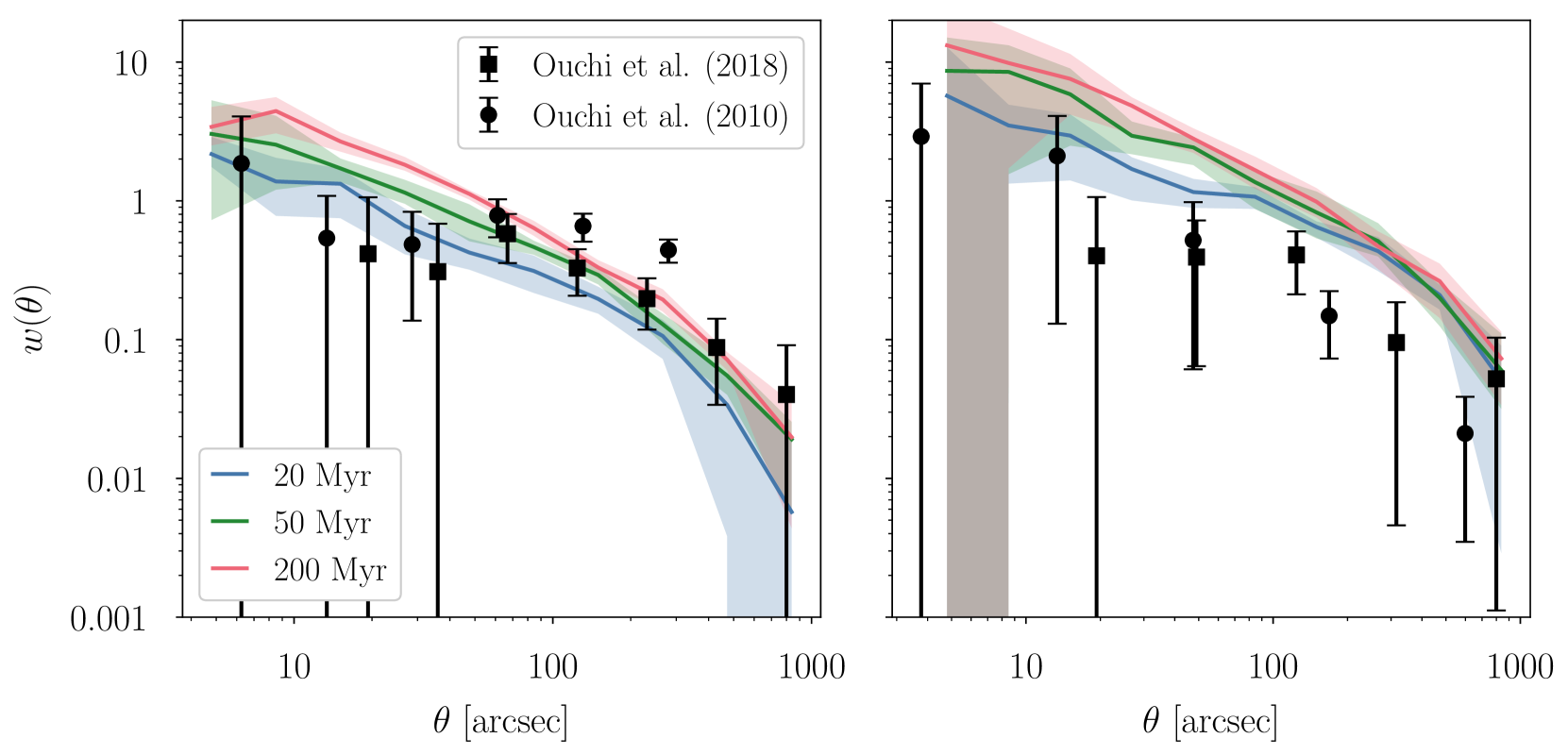
Figure 12: Angular correlation functions at $z=5.756$ and 6.604, comparing different choices of the $\Delta t$ duty cycle parameter: a smaller value of 20 Myr in blue, our fiducial value of 50 Myr in green, and the fiducial value of Trenti et al. (2010) in red. All lines are calculated for the same reionization history.

3.3 Ly $\alpha$ luminosity function evolution

Given the mock LAE sample for each redshift which includes the IGM transmission fraction and the intrinsic luminosity, we can construct the observed sample using Eq. (11). This allows us to construct the (spatial) luminosity function and compare to observed results. In Figure 7 we show the evolution of the luminosity function for our six reionization histories, using our fiducial $\Delta v\propto v_{\mathrm{circ}}$ model. From left to right the redshift of our mock population increases from $z=5.756$ to $z=7.444$. As described above, the luminosity function is calculated by slicing the simulation volume and taking the mean across the slices for each luminosity bin. The shading represents the 68% scatter around this slice mean.

We see that the reionization history which qualitatively fits the observed data across the available narrowband redshifts is the Delayed Very Late model, suggesting that a later reionization is most consistent (as found in Kulkarni et al., 2018; Planck Collaboration et al., 2018). We note that the most difficult constraint to match is the strong attenuation seen in the $z=7.3$ data. The earlier reionization histories under-predict the IGM attenuation required to match the data at $z=7.3$. Since these datasets require the deepest observations in order to find the very rare LAEs visible at such high redshifts, it is also possible that some of the $z=7.3$ bins are not fully complete and may move up in the future SILVERRUSH data release. Attenuation at $z=7.3$ maybe evidence for an even later start to reionization, even later perhaps than our Very Late model. We also note that there is some inconsistency between the different observed datasets at $z=7.0$, which has been discussed in the literature.

3.4 Clustering evolution

As with the luminosity function calculation, we divide the simulation volume into slices of approximately the same depth as the narrowband surveys (10 slices of depth 32 cMpc/h), and assume the same luminosity cuts. We then use the Landy & Szalay (1993) estimator:

$$w(\theta)=\frac{DD(\theta)-2DR(\theta)+RR(\theta)}{RR(\theta)},$$ (13)

to calculate the angular correlation function $w(\theta)$, where $DD(\theta)$ is the number of galaxy-galaxy pairs at separation theta, $RD(\theta)$ the number of random-galaxy pairs, and $RR(\theta)$ the random-random pairs, all of which are normalized appropriately. We employ the swot code (Coupon et al., 2012) to perform the calculation efficiently. Our random field is generated by drawing from a uniform distribution, with similar number density to that of Ouchi et al. (2018) (see Coupon et al., 2018). In Figure 8 we plot the angular correlation function for each test redshift, showing the different reionization histories as in Figure 7. The scatter across the slices is shown by the shading, whilst the lines are the mean value of $w(\theta)$. We note that at both $z=5.756$ (left) and $z=6.604$ (middle-left) our predictions are within the scatter of the observational results from Ouchi et al. (2018). In the $z=6.604$ panel, we already start to see the effect of the different transmission fractions predicted by the reionization history models. The Very Late model, with the lowest average transmission, gives the highest clustering signal.

Considering the SILVERRUSH clustering data (Ouchi et al., 2018, 2010) alone, there is very little evolution in the angular correlation function. Since we expect the clustering to be increased due both to the higher bias at higher redshifts as well as due to the ionized bubble structure of the IGM, this lack of evolution between $z=5.7$ and 6.6 is puzzling, perhaps suggesting that samples are not yet large enough for an accurate determination of the clustering of this higher redshift. From the modelling perspective, it would be possible to reduce the predicted clustering signal at $z=6.6$ further by using a shorter duty cycle, i.e. a lower value of $\Delta t$, however this will also affect the quality of the agreement at $z=5.7$.

3.5 Clustering predictions for $z\geq 7.0$

In the right-hand two panels of Figure 8 we make predictions for the clustering signal at redshifts $z=6.860$ and $=7.444$, which are close to the narrowband filters NB973 and NB101. We see a similar pattern as was observed for the left-hand panels: the clustering signal increases for all models, and in particular the HM12 history (in blue) exhibits the least clustering whilst the Very Late model (in orange) exhibits the most. On intermediary scales these models are non-overlapping at the 68% scatter level. In particular the 2-point correlation function is a function of the reionization history, suggesting that measurements at these redshifts could be strongly constraining.

Apart from the angular correlation function, the clustering signal might also be useful for understanding ionized bubble structure deep into reionization (e.g. Kakiichi et al., 2016). As an example of how this might be possible, we plot a projected mock LAE slice in Figure 9 indicating the intrinsic population in grey and the observed population in red, at $z=6.604$ for the Very Late reionization history. We also plot a contour partioning the map based on the projected ionization fraction, to indicate where the LAEs reside with respect to the ionized bubbles. We note that the observed LAEs seem to lie within ionized bubbles, whereas the unobserved objects are in neutral regions. This configuration could therefore allow us to constrain bubble sizes, perhaps in concert with proposed 21 cm methods (Giri et al., 2018). We leave the construction of such methods to future work.

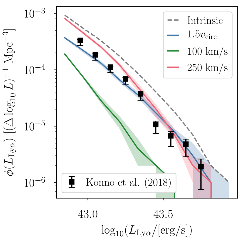
Figure 13: Luminosity functions at $z=5.756$, comparing different choices for the $\Delta v$ emission parameter: our fiducial 1.5 $v_{\mathrm{vcirc}}$ in blue, a fixed value of 100 km/s in green, and a fixed value of 250 km/s in red. All lines are calculated using the same reionization history.

3.6 Differential evolution of the bright and faint end of the luminosity function

In Figure 10 we plot a 2D histogram for the mock LAE population at $z=7.444$, binning by transmission fraction and ‘intrinsic’ Ly $\alpha$ luminosity. We see that for our chosen transmission model the brighter LAEs are preferentially more visible than the fainter objects. In particular the mean and median transmission fractions are shown with the red and white lines, and we see that both curve towards higher transmission fractions as the luminosity increases.

Considering the results of Weinberger et al. (2018), there are two components of this differential visibility to understand. Firstly the absolute transmission fraction at a given redshift is strongly dependent on the emission profile; for our models it is therefore dependent on the choice of $\Delta v$. Our choice in this work assumes $\Delta v\propto v_{\mathrm{circ}}$ which means that $\Delta v\propto M_{\mathrm{vir}}^{\frac{1}{3}}$. This partly explains the behaviour seen in Figure 10; other theoretical work such as Mason et al. (2018) assumed $\Delta v\propto M_{\mathrm{vir}}$ and found a similar boost in the transmission of bright LAEs. However in Weinberger et al. (2018) it was found that there can also be a differential visibility for the relative transmission fraction (i.e. the transmission fraction at a given redshift relative to another redshift). The differential evolution of this relative transmission was partly caused by the presence of brighter LAEs within larger ionized regions, as well as the different host environments of the haloes that the LAEs resided in. Importantly it was found that this differential evolution of the relative transmission was insensitive to the choice of $\Delta v$.

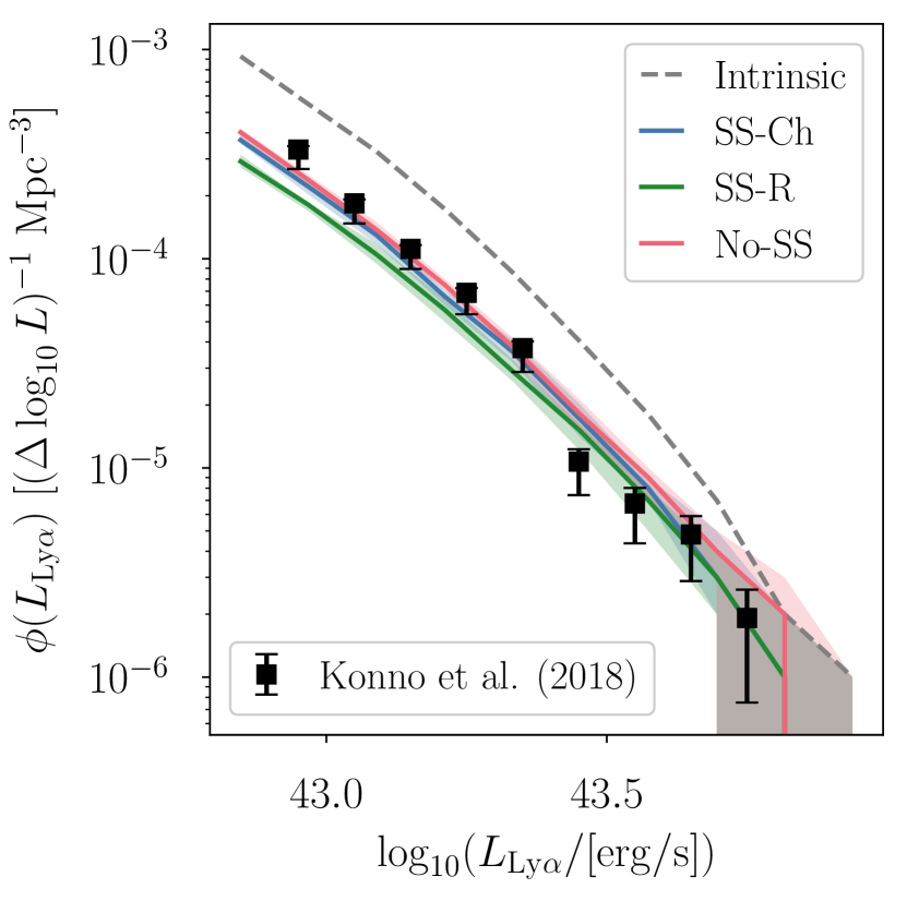
Figure 14: Luminosity functions at $z=5.756$, comparing different self-shielding prescriptions: our fiducial Chardin et al. (2018) based choice in blue, the prescription of Rahmati et al. (2013) in green, and also using no self-shielding prescription in red. All lines are calculated using the same reionization history.

3.7 Typical LAE masses

In Figure 11 we plot the distribution of host halo masses as a function of ‘observed’ Ly $\alpha$ luminosity for our mock population at $z=5.756$. Overplotted on our model histogram we show the observed NB816 data from Khostovan et al. (2018) with a white marker. As in Figure 10 the mean and median of the distributions are shown in red and white lines. We see the strong correlation between halo mass and luminosity, expected from Eq (1), which prevails even after IGM attenuation. The mean host halo mass of our $z=5.756$ mock sample is $10^{11.0}M_{\odot}$, whilst the minimum is $10^{10.3}M_{\odot}$ and the maximum is $10^{12.6}M_{\odot}$.

4 Discussion

Our model, detailed above, reproduces the evolution of the LAE luminosity function and angular correlation function reasonably well. The main free parameters were chosen in our fiducial model as $\Delta v=1.5v_{\mathrm{circ}}$ and $\Delta t=50$ Myr. We now discuss further the motivation for these choices, and the effect of varying these parameters on the observables.

4.1 The effect of varying $\Delta t$ on the clustering

In Figure 12 we show the the angular correlation function at $z=5.756$ and 6.604 for three different values of $\Delta t$: 20, 50 and 200 Myr. We see that increasing this parameter causes an increase in the clustering power, especially at smaller scales. In particular comparing to observations from Ouchi et al. (2018, 2010), the 200 Myr duty cycle causes too much small scale correlation to be consistent with the observed correlation at scales around $10\lesssim\theta\lesssim 60$ arcsec.

As discussed in section 2.2, the $\Delta t$ parameter controls the LBG duty cycle, weighting the abundance matching step towards haloes that have undergone a change in mass within the past $\Delta t$ epoch. The motivation for this prescription is that such variation might correlate with recent bursts of star formation, and therefore UV luminosity and observability. Trenti et al. (2010) chose as their fiducial value $\Delta t=200$ Myr, however we see that in our implementation this does not match the SILVERRUSH clustering signal. We also note that LAE selected galaxies tend to have younger ages than LBG selected populations (Gawiser et al., 2007).

We note again that the absence of any evolution in the observational data across these redshifts is puzzling. Even the $\Delta t=20$ Myr duty cycle model does not achieve a low enough clustering to match the observations at $z=6.6$.

We find that the luminosity function is insensitive to these tested variations in $\Delta t$.

4.2 The effect of varying $\Delta v$ on the luminosity function

In Figure 13 we show the luminosity function at $z=5.756$, and the effect of varying the $\Delta v$ parameter. As the transmission fraction is a strong function of the intrinsic emission profile (Dijkstra et al., 2011), the luminosity function is also dependent on our assumptions about this profile. We see that a fixed value of $\Delta v$ does not fit well; for example the use of $\Delta v=250$ km/s shown in red does fit the bright end reasonable well but overpredicts the number density of LAEs at the faint end. Fixing to a lower value, for example the fiducial choice of Weinberger et al. (2018) of $\Delta v=100$ km/s, results in too much attenuation by the IGM at all luminosities. Our fiducial choice in this work was to set $\Delta v\propto v_{\mathrm{circ}}$, which means that it scales with the LAE host halo mass as $\propto M_{h}^{1/3}$. Due to our population modelling (described in section 2.2–2.4) the LAE luminosity should scale with the UV luminosity (with some stochasticity due to the REW distribution), and hence the host halo mass. This leads to the transmission distribution seen in Figure 10 and the good agreement in Figure 13.

4.3 The effect of self-shielding on the luminosity function

Finally in Figure 14 we show the luminosity function at $z=5.756$, and the effect of varying the self-shielding prescription. Here we compare our fiducial self-shielding prescription with the cases of no self-shielding or a Rahmati et al. (2013) prescription. We see that our luminosity function predictions are largely insensitive to the choice of prescription, although there is some increase in attenuation when self-shielding is added. We note that the non-negligible attenuation is present even in the absence of self-shielding; this is due to the non-zero neutral fraction that is found in photoionization equilibrium at the outskirts of the halo.

5 Conclusions

In conclusion we have built an empirically constrained, self-consistent model of the evolution of LAEs in the epoch of reionization. This modelling made use of the halo population in the state-of-the-art Sherwood simulations, and the hydrodynamic gas structure for quantifying the transmission of Ly $\alpha$ emission through the IGM.

• We used the best fit REW probability distribution of Dijkstra & Wyithe (2012) to model the intrinsic REW distribution of our mock LAE population, and found that incorporating the IGM transmission fraction (calculated for each LAE individually) we reproduced the observed $z=5.7$ REW distribution. Our transmission modelling assumes that the intrinsic LAE emission is a single Gaussian peak, with a velocity offset proportional to the host halo virial circular velocity. This gives a transmission fraction probability distribution across the mock population which corrects the overabundance of high equivalent widths predicted by the Dijkstra & Wyithe (2012) distribution at this redshift.

• In both our original reionization histories and the delayed-end versions, there is sufficient neutral hydrogen in the CGM and infalling gas further surrounding the halo at $z\sim 5.7$ that there is some attenuation redwards of Ly $\alpha$. The attenuation by the neutral hydrogen in the CGM dominates (near the end of reionization) over the attenuation due to the large-scale IGM, even with the presence of residual neutral islands in the delayed-end models (when the average neutral fraction is non-zero). However at higher redshifts around the midpoint of reionization (when $Q\lesssim 0.5$) we find that variations in the neutral fraction of the wider IGM have a dominant effect on the Ly $\alpha$ transmission compared to the CGM neutral gas.

• Using this model we generated mock LAE populations at the redshifts of interest for narrowband surveys, and made predictions for the luminosity function and angular correlation function. Comparing these predictions with current data, in particular from the SILVERRUSH survey, we find that a rather late reionization history (our Very Late model) is in best agreement.

• In order to match the luminosity function across redshifts, we find that the delayed-end Very Late model has the best fitting evolution whilst still able to attenuate the signal enough at the highest redshifts.

• Employing a duty cycle in our LBG modelling allowed us to match the LAE 2-point correlation function with our mock population at $z=5.7$. Our predictions for higher redshifts suggest that the ionization structure of the IGM can enhance the clustering signal significantly already at $z=6.6$. The lack of evolution in the current observed clustering at these redshifts is difficult to explain consistently with the evolution in the luminosity function and equivalent width distribution, and may suggest that the clustering at this redshift has not been measured with sufficient accuracy to extract the effect of reionization.

• In agreement with the results of Weinberger et al. (2018), which found that comparing more and less massive host haloes there is a differential evolution in the relative transmission fraction (e.g. $T_{\mathrm{IGM}}(z)/T_{\mathrm{IGM}}(z=5.7)$), we find that our transmission model also leads to a difference in the absolute transmission (e.g. $T_{\mathrm{IGM}}(z)$). We find that the more luminous LAEs are preferentially less attenuated by the IGM neutral fraction, albeit with a large scatter.

Lyman-$\alpha$ emitting galaxies have been considered as probes of reionization for over 20 years, and many attempts have been made at observing and modelling their behaviour at high redshifts. The ongoing ambitious Ly $\alpha$ surveys are starting to collect samples sufficiently large to allow us to put tight contraints on the reionization history of hydrogen. We find that the evolution of the luminosity function and angular correlation function are indeed strongly dependent on the reionization history, such that further observations at $z\geq 7$ and future Ly $\alpha$ surveys should allow us to map out in detail the second half ($Q\geq 0.5$) of reionization.

Appendix A Comparing the use of full radiative transfer post-processing with the excursion set based method

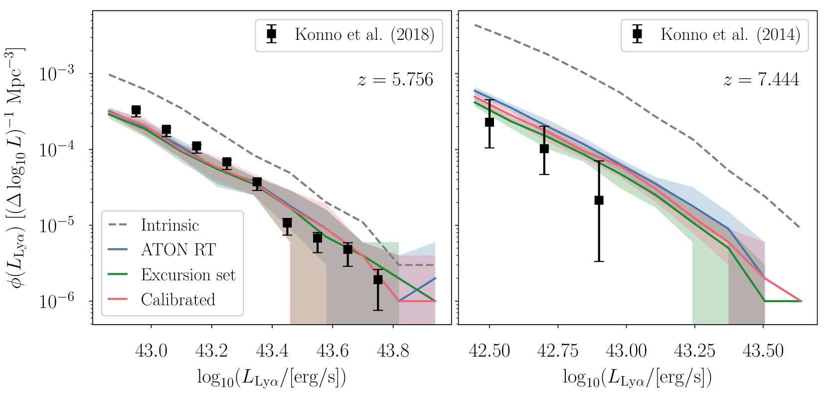
Figure 15: Luminosity function at $z=5.756$ and 7.444 for the same reionization history: calculated using full radiative transfer post-processing in blue, a simple excursion set implementation in green, and using our calibrated excursion set method in red.

In this section we compare three post-processing methods for constructing the large-scale ionization field within the hydrodynamic simulation. We compare (i) a simple excursion set prescription, (ii) the calibrated excursion set method used in Choudhury et al. (2015) (detailed in Weinberger et al. (2018)) and also in this work, and (iii) a full radiative transfer calculation. The full radiative transfer post-processing was performed using the Aton code (Aubert & Teyssier, 2008), as detailed in Kulkarni et al. (2018). All methods were applied to the grids of the $L=160$ cMpc/h, $N=2\times 2048^{3}$ Sherwood simulations to generate the ionized fraction in each grid cell. So that we are comparing like-for-like, we apply the same self-shielding prescription for all three methods to model the small-scale ionization structure. We then generated mock LAE populations as detailed in sections 2.2–2.4 and calculated the observable luminosity function and equivalent width distribution.

In Figure 15 we compare the luminosity functions predicted by these three methods. We show the Aton reionization model of Kulkarni et al. (2018) in blue, the equivalent reionization history implemented with the simple excursion set method in green, and finally our calibrated excursion set method in red. In order to compare like-for-like we have applied the excursion set method in the following two ways: firstly in the simple prescription we have used as inputs the mass-averaged ionized fraction, $\langle x_{\mathrm{HII}}\rangle_{\mathrm{m}}$, and the volume-averaged photoionization rate within ionized regions, $\langle\Gamma_{\mathrm{HI}}\rangle_{\mathrm{v}}$, from the Aton fields. Given these two inputs we can apply the excursion set method and the self-shielding prescription to create the ionization structure at large and small scales. Secondly we have used our calibrated method, in which we take the mass-averaged ionized fraction as before, but instead of using the Aton photoionization rate directly we rather take the mean free path, $\lambda_{\mathrm{mfp}}$, from the Aton fields. This is used to solve for the background photoionization rate consistently within our simulation volume (as detailed in Weinberger et al. (2018), section 2.3).

We find that the three methods give similar predictions, consistent within the 68% scatter across the slices, and that the calibrated method is closer to the full Aton method at all redshifts. When the photoionization rate is $\Gamma_{\mathrm{HI}}\gtrsim 10^{-13}\mathrm{s}^{-1}$ the simple excursion set model is close to the other models, however they start to diverge at higher redshifts when this is no longer the case. We find that the simple excursion set method, which assumes a uniform UV background, slightly overattenuates the luminosity function compared to the Aton method. We note that the full radiative transfer will not have a uniform UV background, and instead we would expect higher photoionization rates near to the LAEs (where also the gas density is highest). This means that when we compare the neutral hydrogen densities around the LAEs, the Aton method gives a more ionized CGM compared to the excursion set method which sees the uniform UV background. This can be seen for $z=7.444$ in Figure 15. For the lower redshifts near to the end of reionization ($z\sim 6$) we find that the photoionization rate is high enough that the ionized fraction saturates, such that the two methods are in good agreement, as seen in the left hand panel. In general our calibrated method predicts slightly higher background photoionization rates which improves the agreement with the Aton results compared to the simple case.

Appendix B Luminosity dependence of the CGM and IGM attenuation

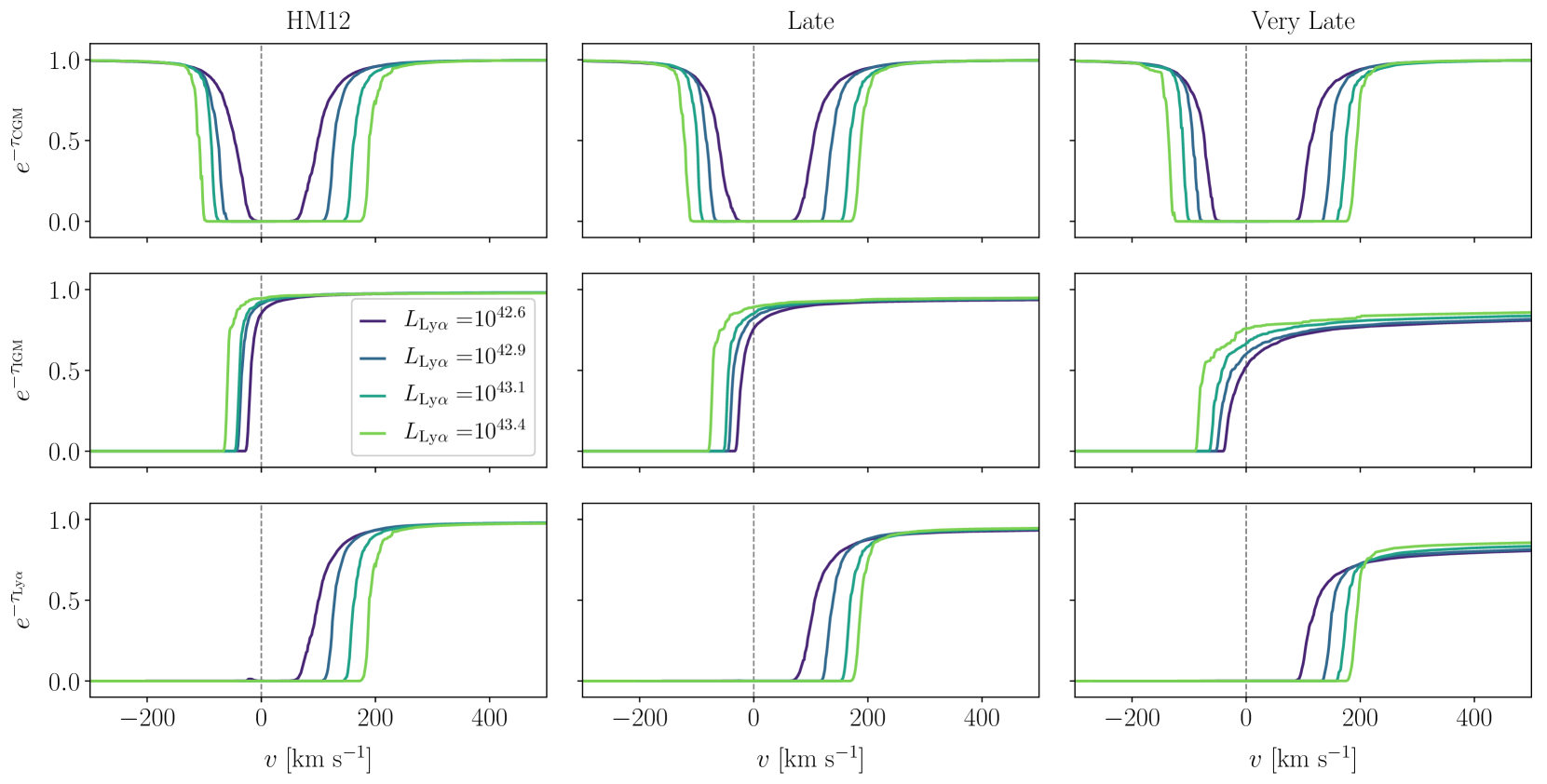
Figure 16: The median transmission in different luminosity bins for the mock LAE population at $z=7.444$, split into CGM (top), IGM (middle) and total (bottom) components as in Figure 6. The different (logarithmic) luminosity bins are indicated by the colour of the lines, with the centre of the bin indicated in the legend. From left to right we show the three original reionization histories: HM12, Late and Very Late.

In section 3.2 we demonstrated that the CGM can play a significant role in the attenuation of Ly $\alpha$, particularly relevant near the end of reionization. However in that section we considered only the median transmission of the full observed sample. We now quantify the variation in the role of CGM/IGM components across luminosity. We note that the Ly $\alpha$ luminosity of our sample broadly scales with the host halo mass (see Figure 11), hence the following also applies to the variation with mass. These results confirm what was found in Weinberger et al. (2018).

In Figure 16 we show the median transmission curves, split into CGM, IGM and total components as in Figure 6, but calculated for samples in different luminosity bins. For brevity we show only the $z=7.444$ original reionization history curves, from left to right showing the HM12, Late and Very Late models respectively. The colour scale of the lines indicates the different luminosity bins, with the faintest bin centred on $10^{42.6}$ erg/s and the brightest centred on $10^{43.4}$ erg/s.

We see in Figure 16 that the attenuation from both the CGM and IGM components depends on luminosity. In particular for the CGM component we see that the fainter objects have more transmission around line-centre, compared to the brightest objects which have a wider absorption trough. This results from higher densities around the more massive haloes, which for the same UV background leads to more neutral gas around the brighter LAEs compared to the faint ones. In contrast for the IGM component, the brighter LAEs have more transmission compared to the faint ones. This is because the brighter LAEs (more massive haloes) reside in larger ionized regions compared to the fainter LAEs. As found in Kakiichi et al. (2016), these different luminosity dependences work against each other in the combined transmission.

Considering a given luminosity bin (one of the colours in Figure 16) we see that the CGM component is similar across the different reionization history models. In comparison the IGM component shows more difference, with the Very Late model in particular showing the most attenuation. This suggests that even with a CGM component that depends on the background photoionization rate, for low enough average ionized fractions (at high enough redshifts into the second half of reionization) the LAE transmission is indeed a strong function of the IGM neutral fraction, and hence LAE observations can provide good constraints.

We note finally that our modelling of the CGM makes various simplifying assumptions which may start to break down in the brightest LAEs. In particular we do not model the source emissivity when calculating the neutral hydrogen density around the halo. Furthermore with our assumption of an intrinsic emission profile we ignore the gas within $R_{\mathrm{vir}}$ of the halo centre. These limitations may affect the CGM transmission for the most massive (brightest) haloes.

Appendix C Reionization history parameters

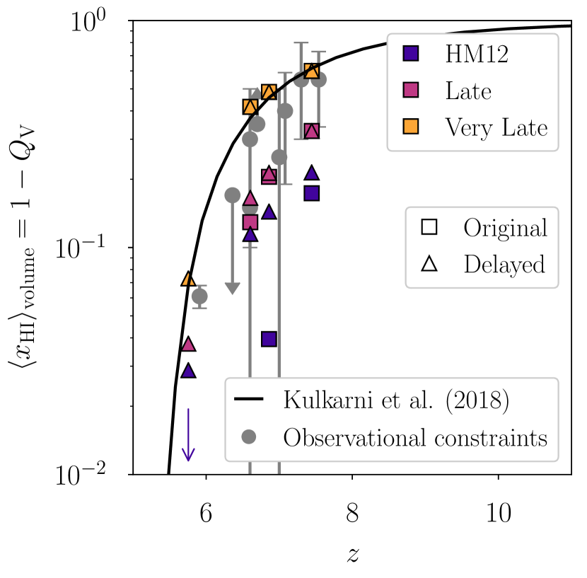
Figure 17: The volume-averaged neutral fraction predicted in our models shown in squares (original histories) and triangles (delayed-end histories), compared to recent observational constraints from a variety of studies, shown with grey circles. These correspond to measurements of LAEs (Konno et al., 2018, $z=6.6$), (Konno et al., 2014, $z=7.3$), (Ouchi et al., 2018, $z=6.6$), (Itoh et al., 2018, $z=7$); QSOs (Greig et al., 2017, $z=7.1$), (Bañados et al., 2018, $z=7.5$); and GRBs (Totani et al., 2016, $z=5.9$), (Totani et al., 2006, $z=6.4$), (Greiner et al., 2009, $z=6.7$). The black solid line shows the model of Kulkarni et al. (2018), which is similar to our delayed-end Very Late model, and was found to reproduce the opacity fluctuations in the Ly $\alpha$ forest. The vertical scale of this figure is logarithmic.

Table 2: Volume-averaged neutral fractions, $\langle x_{\mathrm{HI}}\rangle_{\mathrm{v}}$, for the reionization histories considered in this work.

		Original			Delayed
$z$	HM12	Late	Very Late	HM12	Late	Very Late
5.756	0.0000	0.0000	0.0000	0.0288	0.0377	0.0731
6.604	0.0000	0.1294	0.4168	0.1148	0.1654	0.4168
6.860	0.0395	0.2049	0.4849	0.1440	0.2132	0.4849
7.444	0.1734	0.3263	0.5999	0.2142	0.3263	0.5999

Table 3: Calibrated background photoionization rates, $\log_{10}(\Gamma_{\mathrm{HI}}/\mathrm{s}^{-1})$, for the reionization histories considered in this work.

		Original			Delayed
$z$	HM12	Late	Very Late	HM12	Late	Very Late
5.756	-12.50	-12.61	-12.64	-13.45	-13.47	-13.32
6.604	-12.79	-13.04	-13.26	-13.26	-13.24	-13.26
6.860	-12.88	-13.14	-13.26	-13.25	-13.21	-13.26
7.444	-13.07	-13.21	-13.27	-13.30	-13.20	-13.27

Our reionization prescription takes as input a reionization history given in terms of the mass-averaged ionized fraction evolution with redshift. However observers usually infer the volume-averaged fraction, which is weighted more towards volume-filling voids. In order to convert between the two quantities in practice is difficult; in the case of our simulations we can use a given snapshot (which is a realization of the mass distribution) in order to measure both quantities.

In Table 2 we show for each of our reionization history models the values of the volume-averaged neutral fraction, and similarly in Table 3 the photoionization rates, at the redshifts we considered in this work. In Figure 17 we compare these values to a selection of observational constraints on the average neutral fraction of the IGM, on a logarithmic scale. These constraints were derived from observations of LAEs (Konno et al., 2018, 2014; Ouchi et al., 2018; Itoh et al., 2018), QSOs (Greig et al., 2017; Bañados et al., 2018) and GRBs (Totani et al., 2016, 2006; Greiner et al., 2009). We note that the points representing our reionization histories are not constraints but predictions of the models. The squares show the evolution in our original reionization histories, whilst the triangles show the delayed-end histories. Note that the delayed-end histories only deviate near the end of reionization, so for example the delayed-end Very Late model has the same neutral fraction evolution as the original for $z>6$. The arrow indicates that because the original models have reionized by $z=6$ (Late/Very Late) or $z=6.7$ (HM12), the lower redshift datapoints where $\langle x_{\mathrm{HI}}\rangle_{\mathrm{v}}=0$ are not visible within the logarithmic scale of the figure. We also show with a solid black curve the reionization history model of Kulkarni et al. (2018) which was able to match opacity fluctuations in the Ly $\alpha$ forest, and note that it is very similar to our successful delayed-end Very Late model. In particular we highlight that both versions of our Very Late model are consistent with the SILVERRUSH observational constraints.

References

- Ando et al. (2007) Ando M., Ohta K., Iwata I., Akiyama M., Aoki K., Tamura N., 2007, Publications of the Astronomical Society of Japan, 59, 717
- Aubert & Teyssier (2008) Aubert D., Teyssier R., 2008, MNRAS, 387, 295
- Bañados et al. (2018) Bañados E., et al., 2018, Nature, 553, 473
- Bagley et al. (2017) Bagley M. B., et al., 2017, ApJ, 837, 11
- Behnel et al. (2011) Behnel S., Bradshaw R., Citro C., Dalcin L., Seljebotn D. S., Smith K., 2011, Computing in Science Engineering, 13, 31
- Bhowmick et al. (2018) Bhowmick A. K., Campbell D., DiMatteo T., Feng Y., 2018, preprint, (arXiv:1806.10612)
- Bolton & Haehnelt (2007) Bolton J. S., Haehnelt M. G., 2007, MNRAS, 374, 493
- Bolton & Haehnelt (2013) Bolton J. S., Haehnelt M. G., 2013, MNRAS, 429, 1695
- Bolton et al. (2017) Bolton J. S., Puchwein E., Sijacki D., Haehnelt M. G., Kim T.-S., Meiksin A., Regan J. A., Viel M., 2017, MNRAS, 464, 897
- Bouwens et al. (2008) Bouwens R. J., Illingworth G. D., Franx M., Ford H., 2008, ApJ, 686, 230
- Bouwens et al. (2015) Bouwens R. J., et al., 2015, ApJ, 803, 34
- Calverley et al. (2011) Calverley A. P., Becker G. D., Haehnelt M. G., Bolton J. S., 2011, MNRAS, 412, 2543
- Chardin et al. (2018) Chardin J., Kulkarni G., Haehnelt M. G., 2018, MNRAS,
- Choudhury et al. (2009) Choudhury T. R., Haehnelt M. G., Regan J., 2009, MNRAS, 394, 960
- Choudhury et al. (2015) Choudhury T. R., Puchwein E., Haehnelt M. G., Bolton J. S., 2015, MNRAS, 452, 261
- Coupon et al. (2012) Coupon J., et al., 2012, A&A, 542, A5
- Coupon et al. (2018) Coupon J., Czakon N., Bosch J., Komiyama Y., Medezinski E., Miyazaki S., Oguri M., 2018, Publications of the Astronomical Society of Japan, 70, S7
- Dayal et al. (2009) Dayal P., Ferrara A., Saro A., Salvaterra R., Borgani S., Tornatore L., 2009, MNRAS, 400, 2000
- Diener et al. (2017) Diener C., et al., 2017, MNRAS, 471, 3186
- Dijkstra (2014) Dijkstra M., 2014, Publ. Astron. Soc. Australia, 31, e040
- Dijkstra & Westra (2010) Dijkstra M., Westra E., 2010, MNRAS, 401, 2343
- Dijkstra & Wyithe (2012) Dijkstra M., Wyithe J. S. B., 2012, MNRAS, 419, 3181
- Dijkstra et al. (2006) Dijkstra M., Haiman Z., Spaans M., 2006, ApJ, 649, 14
- Dijkstra et al. (2007) Dijkstra M., Lidz A., Wyithe J. S. B., 2007, MNRAS, 377, 1175
- Dijkstra et al. (2011) Dijkstra M., Mesinger A., Wyithe J. S. B., 2011, MNRAS, 414, 2139
- Faucher-Giguère et al. (2009) Faucher-Giguère C.-A., Lidz A., Zaldarriaga M., Hernquist L., 2009, ApJ, 703, 1416
- Furlanetto et al. (2004) Furlanetto S. R., Zaldarriaga M., Hernquist L., 2004, ApJ, 613, 1
- Gawiser et al. (2007) Gawiser E., et al., 2007, ApJ, 671, 278
- Giri et al. (2018) Giri S. K., Mellema G., Dixon K. L., Iliev I. T., 2018, MNRAS, 473, 2949
- Greig et al. (2017) Greig B., Mesinger A., Haiman Z., Simcoe R. A., 2017, MNRAS, 466, 4239
- Greiner et al. (2009) Greiner J., et al., 2009, ApJ, 693, 1610
- Gronke & Dijkstra (2016) Gronke M., Dijkstra M., 2016, ApJ, 826, 14
- Gunn & Peterson (1965) Gunn J. E., Peterson B. A., 1965, ApJ, 142, 1633
- Gurung López et al. (2018) Gurung López S., Orsi Á. A., Bonoli S., Baugh C. M., Lacey C. G., 2018, preprint, (arXiv:1807.00006)
- Hashimoto et al. (2015) Hashimoto T., et al., 2015, ApJ, 812, 157
- Hassan et al. (2016) Hassan S., Davé R., Finlator K., Santos M. G., 2016, MNRAS, 457, 1550
- Hu et al. (2016) Hu E. M., Cowie L. L., Songaila A., Barger A. J., Rosenwasser B., Wold I. G. B., 2016, ApJ, 825, L7
- Hunter (2007) Hunter J. D., 2007, Computing in Science Engineering, 9, 90
- Hutter et al. (2014) Hutter A., Dayal P., Partl A. M., Müller V., 2014, MNRAS, 441, 2861
- Hutter et al. (2015) Hutter A., Dayal P., Müller V., 2015, MNRAS, 450, 4025
- Inoue et al. (2018) Inoue A. K., et al., 2018, PASJ,
- Itoh et al. (2018) Itoh R., et al., 2018, preprint, (arXiv:1805.05944)
- Jensen et al. (2013) Jensen H., Laursen P., Mellema G., Iliev I. T., Sommer-Larsen J., Shapiro P. R., 2013, MNRAS, 428, 1366
- Jensen et al. (2014) Jensen H., Hayes M., Iliev I. T., Laursen P., Mellema G., Zackrisson E., 2014, MNRAS, 444, 2114
- Jones et al. (2001) Jones E., Oliphant T., Peterson P., et al., 2001, SciPy: Open source scientific tools for Python, http://www.scipy.org/
- Kakiichi et al. (2016) Kakiichi K., Dijkstra M., Ciardi B., Graziani L., 2016, MNRAS, 463, 4019
- Kashikawa et al. (2006) Kashikawa N., et al., 2006, ApJ, 648, 7
- Kashikawa et al. (2011) Kashikawa N., et al., 2011, ApJ, 734, 119
- Khostovan et al. (2018) Khostovan A. A., et al., 2018, preprint, p. arXiv:1811.00556 (arXiv:1811.00556)
- Konno et al. (2014) Konno A., et al., 2014, ApJ, 797, 16
- Konno et al. (2018) Konno A., et al., 2018, PASJ, 70, S16
- Kulkarni et al. (2016) Kulkarni G., Choudhury T. R., Puchwein E., Haehnelt M. G., 2016, MNRAS, 463, 2583
- Kulkarni et al. (2018) Kulkarni G., Keating L. C., Haehnelt M. G., Bosman S. E. I., Puchwein E., Chardin J., Aubert D., 2018, preprint, p. arXiv:1809.06374 (arXiv:1809.06374)
- Landy & Szalay (1993) Landy S. D., Szalay A. S., 1993, ApJ, 412, 64
- Laursen et al. (2009) Laursen P., Sommer-Larsen J., Andersen A. C., 2009, ApJ, 704, 1640
- Laursen et al. (2011) Laursen P., Sommer-Larsen J., Razoumov A. O., 2011, ApJ, 728, 52
- Laursen et al. (2018) Laursen P., Sommer-Larsen J., Milvang-Jensen B., Fynbo J. P. U., Razoumov A. O., 2018, preprint, p. arXiv:1806.07392 (arXiv:1806.07392)
- Lee et al. (2009) Lee K.-S., Giavalisco M., Conroy C., Wechsler R. H., Ferguson H. C., Somerville R. S., Dickinson M. E., Urry C. M., 2009, ApJ, 695, 368
- Madau & Rees (2000) Madau P., Rees M. J., 2000, ApJ, 542, L69
- Mainali et al. (2018) Mainali R., et al., 2018, MNRAS, p. 1569
- Mason et al. (2018) Mason C. A., et al., 2018, ApJ, 857, L11
- Matthee et al. (2015) Matthee J., Sobral D., Santos S., Röttgering H., Darvish B., Mobasher B., 2015, MNRAS, 451, 400
- Matthee et al. (2017) Matthee J., Sobral D., Darvish B., Santos S., Mobasher B., Paulino- Afonso A., Röttgering H., Alegre L., 2017, MNRAS, 472, 772
- Matthee et al. (2018) Matthee J., Sobral D., Gronke M., Paulino- Afonso A., Stefanon M., Röttgering H., 2018, preprint, p. arXiv:1805.11621 (arXiv:1805.11621)
- Mesinger & Furlanetto (2007) Mesinger A., Furlanetto S., 2007, Astrophys. J., 669, 663
- Mesinger et al. (2011) Mesinger A., Furlanetto S., Cen R., 2011, MNRAS, 411, 955
- Mesinger et al. (2015) Mesinger A., Aykutalp A., Vanzella E., Pentericci L., Ferrara A., Dijkstra M., 2015, MNRAS, 446, 566
- Miyazaki et al. (2002) Miyazaki S., et al., 2002, Publications of the Astronomical Society of Japan, 54, 833
- Miyazaki et al. (2012) Miyazaki S., et al., 2012, in Ground-based and Airborne Instrumentation for Astronomy IV. p. 84460Z, doi:10.1117/12.926844
- Murray et al. (2013) Murray S. G., Power C., Robotham A. S. G., 2013, Astronomy and Computing, 3, 23
- Nakajima et al. (2018) Nakajima K., Fletcher T., Ellis R. S., Robertson B. E., Iwata I., 2018, MNRAS, 477, 2098
- Neufeld (1990) Neufeld D. A., 1990, ApJ, 350, 216
- Ono et al. (2012) Ono Y., et al., 2012, ApJ, 744, 83
- Ota et al. (2017) Ota K., et al., 2017, ApJ, 844, 85
- Ouchi et al. (2008) Ouchi M., et al., 2008, ApJS, 176, 301
- Ouchi et al. (2010) Ouchi M., et al., 2010, ApJ, 723, 869
- Ouchi et al. (2018) Ouchi M., et al., 2018, Publications of the Astronomical Society of Japan, 70, S13
- Partridge & Peebles (1967) Partridge R. B., Peebles P. J. E., 1967, ApJ, 147, 868
- Pentericci et al. (2014) Pentericci L., et al., 2014, ApJ, 793, 113
- Planck Collaboration et al. (2014) Planck Collaboration et al., 2014, A&A, 571, A16
- Planck Collaboration et al. (2016) Planck Collaboration Adam R., Aghanim N., Ashdown M., Aumont J., Baccigalupi C., et al. 2016, A&A, 596, A108
- Planck Collaboration et al. (2018) Planck Collaboration Aghanim N., Akrami Y., Ashdown M., Aumont J., et al. 2018, preprint, p. arXiv:1807.06209 (arXiv:1807.06209)
- Puchwein et al. (2018) Puchwein E., Haardt F., Haehnelt M. G., Madau P., 2018, preprint, (arXiv:1801.04931)
- Rahmati et al. (2013) Rahmati A., Pawlik A. H., Raičevic̀ M., Schaye J., 2013, MNRAS, 430, 2427
- Rosdahl et al. (2018) Rosdahl J., et al., 2018, MNRAS, 479, 994
- Sadoun et al. (2017) Sadoun R., Zheng Z., Miralda-Escudé J., 2017, ApJ, 839, 44
- Santos et al. (2010) Santos M. G., Ferramacho L., Silva M. B., Amblard A., Cooray A., 2010, MNRAS, 406, 2421
- Santos et al. (2016) Santos S., Sobral D., Matthee J., 2016, MNRAS, 463, 1678
- Schenker et al. (2012) Schenker M. A., Stark D. P., Ellis R. S., Robertson B. E., Dunlop J. S., McLure R. J., Kneib J.-P., Richard J., 2012, ApJ, 744, 179
- Sheth et al. (2001) Sheth R. K., Mo H. J., Tormen G., 2001, MNRAS, 323, 1
- Shibuya et al. (2014) Shibuya T., et al., 2014, ApJ, 788, 74
- Shibuya et al. (2018) Shibuya T., et al., 2018, Publications of the Astronomical Society of Japan, 70, S14
- Smith et al. (2018) Smith A., Ma X., Bromm V., Finkelstein S. L., Hopkins P. F., Faucher- Giguère C.-A., Kereš D., 2018, preprint, p. arXiv:1810.08185 (arXiv:1810.08185)
- Sobral et al. (2015) Sobral D., Matthee J., Darvish B., Schaerer D., Mobasher B., Röttgering H. J. A., Santos S., Hemmati S., 2015, ApJ, 808, 139
- Sobral et al. (2017) Sobral D., et al., 2017, preprint, p. arXiv:1710.08422 (arXiv:1710.08422)
- Springel (2005) Springel V., 2005, Monthly Notices of the Royal Astronomical Society, 364, 1105
- Springel et al. (2001) Springel V., Yoshida N., White S. D. M., 2001, New Astron., 6, 79
- Stark et al. (2010) Stark D. P., Ellis R. S., Chiu K., Ouchi M., Bunker A., 2010, MNRAS, 408, 1628
- Stark et al. (2011) Stark D. P., Ellis R. S., Ouchi M., 2011, ApJ, 728, L2
- Steidel et al. (2010) Steidel C. C., Erb D. K., Shapley A. E., Pettini M., Reddy N., Bogosavljević M., Rudie G. C., Rakic O., 2010, ApJ, 717, 289
- Totani et al. (2006) Totani T., Kawai N., Kosugi G., Aoki K., Yamada T., Iye M., Ohta K., Hattori T., 2006, Publications of the Astronomical Society of Japan, 58, 485
- Totani et al. (2016) Totani T., Aoki K., Hattori T., Kawai N., 2016, Publications of the Astronomical Society of Japan, 68, 15
- Trenti & Stiavelli (2009) Trenti M., Stiavelli M., 2009, ApJ, 694, 879
- Trenti et al. (2010) Trenti M., Stiavelli M., Bouwens R. J., Oesch P., Shull J. M., Illingworth G. D., Bradley L. D., Carollo C. M., 2010, ApJ, 714, L202
- Verhamme et al. (2006) Verhamme A., Schaerer D., Maselli A., 2006, A&A, 460, 397
- Verhamme et al. (2018) Verhamme A., et al., 2018, MNRAS, 478, L60
- Weinberger et al. (2018) Weinberger L. H., Kulkarni G., Haehnelt M. G., Choudhury T. R., Puchwein E., 2018, MNRAS, 479, 2564
- Wyithe & Bolton (2011) Wyithe J. S. B., Bolton J. S., 2011, MNRAS, 412, 1926
- Yang et al. (2016) Yang H., Malhotra S., Gronke M., Rhoads J. E., Dijkstra M., Jaskot A., Zheng Z., Wang J., 2016, ApJ, 820, 130
- Zheng & Wallace (2014) Zheng Z., Wallace J., 2014, ApJ, 794, 116
- Zheng et al. (2010) Zheng Z., Cen R., Trac H., Miralda-Escudé J., 2010, ApJ, 716, 574
- Zheng et al. (2017) Zheng Z.-Y., et al., 2017, ApJ, 842, L22
- van der Walt et al. (2011) van der Walt S., Colbert S. C., Varoquaux G., 2011, Computing in Science Engineering, 13, 22