A Robust Riemann Solver for Multiple Hydro-Elastoplastic Solid Mediums

Abstract

We propose a robust approximate solver for the hydro-elastoplastic solid material, a general constitutive law extensively applied in explosion and high speed impact dynamics, and provide a natural transformation between the fluid and solid in the case of phase transitions. The hydrostatic components of the solid is described by a family of general Mie-Grüneisen equation of state (EOS), while the deviatoric component includes the elastic phase, linearly hardened plastic phase and fluid phase. The approximate solver provides the interface stress and normal velocity by an iterative method. The well-posedness and convergence of our solver are proved with mild assumptions on the equations of state. The proposed solver is applied in computing the numerical flux at the phase interface for our compressible multi-medium flow simulation on Eulerian girds. Several numerical examples, including Riemann problems, shock-bubble interactions, implosions and high speed impact applications, are presented to validate the approximate solver.

1 Introduction

Significant interest has arisen in the modeling and simulation of dynamic events that involve high-load conditions and large deformations, such as shock-driven motions, high-speed impacts, implosions, and so on. The numerical analysis of these problems demands the implementation of very specific capabilities that enable the simulation of multiple mediums and their interactions through accurate descriptions of boundary conditions and high-resolution shock and wave capturing.

There are two typical frameworks to describe the motion of multi-medium flows [1], that is, the Lagrangian framework and the Eulerian framework. In the Lagrangian framework, the equations for mass, momentum and energy conservations are solved using a computational mesh that conforms to the material boundaries and moves with particles [2, 3], which benefits from its simplicity and natural description of deformation, but suffers from mesh distortion when dealing with large deformation problems. In Eulerian framework the mesh is fixed in space, which makes these methods very suitable for flows with large deformations, such as Udaykumar et al. [4, 5, 6, 7, 8, 9], Liu et al. [10, 11, 12, 13, 14, 15], Mehmandoust et al. [16], Sijoy et al. [17], and so on. A typical procedure of multi-medium interaction in Eulerian grids mainly consists of two steps. The first step is the interface capture, including the diffuse interface method (DIM) [18, 19, 20, 21, 22, 23], and the sharp interface method (SIM), such as the volume of fluid (VOF) method [24, 25], level set method [26, 27], moment of fluid (MOF) method [28, 29, 30] and front-tracking method [31, 32]. The second step is the accurate prediction of the interface states, which can be used to stabilize the numerical diffusion in diffuse interface methods, and to compute the numerical flux and interface motion in sharp interface methods. One common approach is to solve a multi-medium Riemann problem which contains the fundamentally physical and mathematical properties of the governing equations and plays a key role in designing the numerical flux.

The solution of a multi-medium Riemann problem depends not only on the initial states at each side of the interface, but also on the forms of constitutive relations. There exist some difficulties in the cases of real materials due to the high nonlinearity of the equation of state and non-conservation of the deviatoric evolution. A variety of methods to solve the corresponding Riemann problems have then been proposed. For example, Yadav [33] analyzed spherical shocks in metals by employing a hydrostatic Mie-Grüneisen equation of state that does not consider the effects of shear deformation. Shyue [34] developed a Roe’s approximate Riemann solver for the Mie-Grüneisen EOS with variable Grüneisen coefficient. Arienti et al. [35] applied a Roe-Glaster solver to compute the equations combining the Euler equations involving chemical reaction with the Mie-Grüneisen EOS. Lee et al. [36] developed an exact Riemann solver for the Mie-Grüneisen EOS with constant Grüneisen coefficient, where the integral terms are evaluated using an iterative Romberg algorithm. Banks [37] and Kamm [38] developed a Riemann solver for the convex Mie-Grüneisen EOS by solving a nonlinear equation for the density increment involved in the numerical integration of rarefaction curves. Unlike the fluid, there may exist more than one nonlinear wave in a solid when it undergoes an elastoplastic deformation, which will increase the difficulty to obtain the exact solution of the Riemann problem. Kaboudian et al. [39] analyzed the elastic Riemann problem in the Lagrangian framework, and established the corresponding Riemann solver according to the characteristic theory. Xiao et al. [40] raised an iterative procedure to solve the Riemann problem approximately by linearizing the Riemann invariants. Tang et al. [41] put forward a nearly exact Riemann solver for the perfectly elastoplastic solid based on the physical observation, where the Murnagham EOS and perfectly plastic model were chosen for the hydrostatic pressure and deviatoric stress respectively. Abouziarov et al. [42] and Bazhenov et al. [43] analyzed the structures of shock waves and rarefaction waves in an elastoplastic material on the assumption of barotropy, without taking into account the internal energy equation. Cheng et al. [13, 14] analyzed the wave structures of one-dimensional elastoplastic flows and developed a two-rarefaction approximate Riemann solver. Menshov et al. [44] provided an analysis of the Riemann problem in a complete statement for the perfect plasticity on the assumption of one-dimensional motion and uniaxial strain. Liu et al. [45, 46], Feng et al. [47] and Gao et al. [48, 49] analyzed the exact solution of the elastic-perfectly plastic solid with the Murnagham EOS and stiffened gas EOS, and combined it with the modified ghost fluid method to solve multi-medium problems. Gavirilyuk et al. [50] constructed a Riemann solver for the linearly elastic system of the hyperbolic non-conservative models with transverse waves. In addition, the elastic energy was included in the total energy, and an extra evolution equation, on the basis of Despres et al. [51], was added in order to make the elastic transformation reversible in the absence of shock wave.

In this paper, we propose an approximate multi-medium Riemann solver with a family of general Mie-Grüneisen EOS and hydro-elastoplastic deviatoric deformation, which can provide a smooth transformation between the fluid and solid in the case of phase transitions. The Riemann problem together with its approximate solver in such case, which has not been well studied in the literature yet, can be applied in the numerical scheme developed in [52] conveniently. The study we carried out here is a further exploration of our previous work in [53], which is restricted on the fluid-fluid Riemann solver with Mie-Grüneisen EOS. Similar to the solver in [53], some mild conditions on the coefficients of Mie-Grüneisen EOS are assumed to ensure the convexity of the equation of state, which guarantees the existence and uniqueness of the algebraic equation derived from the Riemann problem. The algebraic equation is derived by a detailed analysis on the structure of the Riemann fan. Then we solve the algebraic equation by an inexact Newton method [54], where the function and its derivatives are evaluated approximately since the analytical expressions are not available. The approximate evaluations of the function and its derivatives are quite involved since they depend on the wave structure and the error estimate in the run time. In spite of its complexity, we find that the convergence of the inexact Newton iteration can be achieved, which is significant to the success of large-scale simulations in engineering applications. To validate the proposed approximate Riemann solver, we employ it in the computation of multi-medium compressible flows with Mie-Grüneisen EOS and elastoplastic deformation. The approximate solver developed here enhances the capacity of the numerical scheme for our multi-medium compressible fluid flows [52, 53], and allows us to simulate the problems with highly nonlinear fluids and elastoplastic solids.

The rest of this paper is arranged as follows. In Section 2, a solution strategy for the multi-medium Riemann problem with Mie-Grüneisen EOS and hydro-elastoplastic deviatoric deformation is presented. In Section 3, the procedures of our approximate Riemann solver are outlined, and the well-posedness and convergence are analyzed. In Section 4, the application of our Riemann solver in multi-medium compressible flow calculations is briefly introduced. In Section 5, several classical Riemann problems and applications for shock-bubble interaction, implosion and high speed impact problems are carried out to validate the accuracy and robustness of our schemes. Finally, a short conclusion is drawn in Section 6.

2 Multi-medium Riemann Problem

The one-dimensional compressible multi-medium Riemann problem, in the absence of heat conduction and radiation, can be written as

$$\dfrac{\partial\bm{U}}{\partial\tau}+\dfrac{\partial\bm{F}(\bm{U})}{\partial\xi}=\bm{0},\quad\bm{U}(\xi,\tau=0)=\begin{cases}\bm{U}_{l},&\xi<0,\\ \bm{U}_{r},&\xi>0.\end{cases}$$ (1)

Here $\tau$ is time, $\xi$ is spatial coordinate. $\bm{U}=[\rho,\rho u,E]^{\top}$ is the vector of conservative variables, and $\bm{F}(\bm{U})=[\rho u,\rho u^{2}-\sigma,(E-\sigma)u]^{\top}$ is the corresponding flux. $\rho$, $u$ and $E$ are the density, velocity and total energy respectively, and $\sigma$ is the normal Cauchy stress of the hydro-elastoplastic solid.

To close the governing equations (1), we need an equation of state or constitutive law to relate the thermodynamic variables. The hydro-elastoplastic model is a general form of nonlinear fluid, elasticity, perfect elastoplasticity and linearly hardened elastoplasticity, as a mix and match combination of isotropic models.

In the hydro-elastoplastic model, the deformation is decomposed into the volumetric deformation and shear deformation, and the Cauchy stress tensor $\bm{\sigma}$ is also divided into the hydrostatic pressure and deviatoric stress tensor respectively,

$$\bm{\sigma}=-p{\bf I}+{\bf S},$$

where $p$ is the hydrostatic pressure, $\bf S$ is the deviatoric stress tensor, and $\bf I$ is the unit tensor.

The hydrostatic pressure $p$ is expressed by the Mie-Grüneisen EOS, which may be varied independently of the deviatoric response and has the following general form

$$p(\rho,e)=\varGamma(\rho)\rho e+h(\rho),$$ (2)

where $e$ is the specific internal energy, $\varGamma(\rho)$ is the Grüneisen coefficient, and $h(\rho)$ is a reference state associated with the cold contribution resulting from the interactions of atoms at rest [55]. For the ease of our analysis, we impose on $\varGamma(\rho)$ and $h(\rho)$ the following assumptions

(C1) $\varGamma^{\prime}(\rho)\leq 0,~{}(\rho\varGamma(\rho))^{\prime}\geq 0,~{}(\rho\varGamma(\rho))^{\prime\prime}\geq 0$;

(C2) $\lim\limits_{\rho\rightarrow+\infty}\varGamma(\rho)=\varGamma_{\infty}>0,~{}\varGamma(\rho)\leq\varGamma_{\infty}+2$;

(C3) $h^{\prime}(\rho)\geq 0,~{}h^{\prime\prime}(\rho)\geq 0$,

similar to our previous work in [53]. A lot of equations of state of our interests fulfill these assumptions. Particularly, we collect some equations of state in Appendix A which are used in our numerical tests as examples.

The deviatoric stress $\bf S$ has a piecewisely complex constitutive relations, which is governed by means of Hooke’s law in the elastic region, the linearly hardened plastic flow rule during the plastic region, and constant states when the plastic limit is violated. The von Mises criterion is adopted to determine whether the material is under elastic region, plastic region or fluid region, which can be written in terms of the deviatoric stress

$${\mathscr{H}}(\mathbf{S},Y)=\mathbf{S}:\mathbf{S}-\dfrac{2}{3}Y^{2},$$

where $Y$ is the yield stress limit of the solid material. $Y=Y^{{}_{\mathscr{E}}}$ corresponds to the elastic yield stress, and $Y=Y^{{}_{\mathscr{P}}}$ stands for the plastic yield stress, respectively.

The evolution of the deviatoric stress tensor can be written in the following piecewise expressions

$$\dfrac{\partial{\mathbf{S}}}{\partial{t}}+\bm{u}\cdot\nabla\mathbf{S}=\left\{\begin{array}[]{ll}2\mu^{{}_{\mathscr{E}}}\left(\mathbf{D}-\dfrac{1}{3}\operatorname{tr}(\mathbf{D})\mathbf{I}\right),&\left|S_{\rm eff}\right|\leq Y^{{}_{\mathscr{E}}},\\ 2\mu^{{}_{\mathscr{P}}}\left(\mathbf{D}-\dfrac{1}{3}\operatorname{tr}(\mathbf{D})\mathbf{I}\right),&Y^{{}_{\mathscr{E}}}<\left|S_{\rm eff}\right|<Y^{{}_{\mathscr{P}}},\\ \bm{0},&\left|S_{\rm eff}\right|=Y^{{}_{\mathscr{P}}},\\ \end{array}\right.$$

where

$$\mathbf{D}=\dfrac{1}{2}\left(\dfrac{\partial{\bm{u}}}{\partial{\bm{x}}}+\left(\dfrac{\partial{\bm{u}}}{\partial{\bm{x}}}\right)^{\top}\right)$$

is the rate of the deformation tensor, $S_{\rm eff}=\sqrt{\frac{3}{2}\mathbf{S}:\mathbf{S}}$ is the effective stress, and $\mu^{{}_{\mathscr{E}}}$ and $\mu^{{}_{\mathscr{P}}}$ are the elastic and plastic shear modulus, respectively.

Utilizing the continuity equation, we can obtain the following balance law

$$\dfrac{\partial{\rho S_{ij}}}{\partial{t}}+\dfrac{\partial{\rho u_{k}S_{ij}}}{\partial{x_{k}}}=\left\{\begin{array}[]{ll}\beta^{{}_{\mathscr{E}}}\left(\dfrac{\partial{u_{i}}}{\partial{x_{j}}}+\dfrac{\partial{u_{j}}}{\partial{x_{i}}}\right)-\dfrac{2}{3}\beta^{{}_{\mathscr{E}}}\delta_{ij}\dfrac{\partial{u_{k}}}{\partial{x_{k}}},&\left|S_{\rm eff}\right|\leq Y^{{}_{\mathscr{E}}},\\ \beta^{{}_{\mathscr{P}}}\left(\dfrac{\partial{u_{i}}}{\partial{x_{j}}}+\dfrac{\partial{u_{j}}}{\partial{x_{i}}}\right)-\dfrac{2}{3}\beta^{{}_{\mathscr{P}}}\delta_{ij}\dfrac{\partial{u_{k}}}{\partial{x_{k}}},&Y^{{}_{\mathscr{E}}}<\left|S_{\rm eff}\right|\leq Y^{{}_{\mathscr{P}}},\\ 0,&\left|S_{\rm eff}\right|=Y^{{}_{\mathscr{P}}},\end{array}\right.$$

where $\beta^{{}_{\mathscr{E}}}=\rho\mu^{{}_{\mathscr{E}}}$, $\beta^{{}_{\mathscr{P}}}=\rho\mu^{{}_{\mathscr{P}}}$, $\delta_{ij}$ is the Dirac function.

Remark 1.

The hydro-elastoplastic model can degenerate to the elastic model, perfectly elastoplastic model, linearly hardened elastoplastic model and fluid model naturally. Fox example, it will degenerate to the elastic model when $\mu^{{}_{\mathscr{E}}}=\mu^{{}_{\mathscr{P}}}$ and $Y^{{}_{\mathscr{E}}}=Y^{{}_{\mathscr{P}}}=\infty$, to the perfectly elastoplastic model when $\mu^{{}_{\mathscr{P}}}=0$ and $Y^{{}_{\mathscr{P}}}=\infty$, to the linearly hardened elastoplasticity when $\mu^{{}_{\mathscr{P}}}<\mu^{{}_{\mathscr{E}}}$ and $Y^{{}_{\mathscr{P}}}=\infty$, and to the fluid model when $\mu^{{}_{\mathscr{P}}}=\mu^{{}_{\mathscr{E}}}=0$ and $Y^{{}_{\mathscr{E}}}=Y^{{}_{\mathscr{P}}}=0$, respectively.

The model presented above is a conventional Eulerian non-conservative model for the elastoplastic behavior, which couples the nonlinear Euler equations of compressible fluids with the augmented elastoplastic deformation. In high-rate and large deformation region, the volumeric deformation is dominant and the deviatoric deformation can be neglected. When the load is removed, the elastoplastic effect should be taken into account again. For elastic deviatoric response the shear moduli may be taken to be functions of temperature and pressure. Plasticity is based on an additive decomposition of the rate of deformation tensor into elastic and plastic parts [56].

Here we discuss the multi-medium Riemann problem between hydro-elastoplastic models, which can be treated in a similar way as the single-medium Riemann problem as long as the materials remain immiscible. The Riemann solution consists of several constant regions separated by the phase interface and genuinely nonlinear waves. The key of the Riemann problem is to compute the states in the region adjacent to the phase interface (the so called star region). To understand the influence of material deformation on the interface states, the solution structure in each medium should be analyzed with consideration of the elastoplastic deformation. Without loss of generality, we take the medium at the right side of the interface as the example, and the left side can be analyzed in a similar manner.

2.1 Solution in the elastic phase

The Riemann solution in the elastic phase consists of two constant states separated by an elastic acoustic wave, whose speed is given by

$$\lambda=u+\sqrt{c^{2}+\dfrac{4\mu^{{}_{\mathscr{E}}}}{3\rho}}.$$

Figure 1: Wave structure of the elastic solid phase in the $\xi-\tau$ space.

Figure 2: Wave structure of the elastoplastic solid phase in the $\xi-\tau$ space.

A typical wave structure for the elastic Riemann problem is shown in Fig. 2. The acoustic wave is genuinely nonlinear, while the contact wave is linearly degenerate [50]. The jump of the normal deviatoric stress $S$ across the acoustic wave satisfies

$$S_{k}^{*}-S_{k}=\dfrac{4\beta^{{}_{\mathscr{E}}}_{k}}{3}\left(\dfrac{1}{\rho_{k}^{*}}-\dfrac{1}{\rho_{k}}\right),$$ (3)

where the superscript “*” stands for the star region state.

• Rarefaction wave

  Denote by $q=p-S$ the negative normal component of Cauchy stress tensor on the interface. If $q_{k}^{*}\leq q_{k}$, the acoustic wave is a rarefaction wave. It can be found that

  $$u-\int\dfrac{1}{\rho}\sqrt{c^{2}+\dfrac{4\beta^{{}_{\mathscr{E}}}}{3\rho^{2}}}\mathrm{d}\rho,\quad p-\int c^{2}\mathrm{d}\rho,$$

  are Riemann invariants, which yield the relation

  $$u^{*}_{k}-u_{k} =\displaystyle\int_{q_{k}}^{q^{*}_{k}}\left(\rho^{2}c^{2}+\dfrac{4}{3}\beta^{{}_{\mathscr{E}}}_{k}\right)^{1/2}\mathrm{d}q,$$

  $$\rho_{k}^{*}-\rho_{k} =\displaystyle\int_{p_{k}}^{p_{k}^{*}}\dfrac{\mathrm{d}p}{c^{2}}.$$

• Shock wave

  If $q_{k}^{*}>q_{k}$, then the acoustic wave is a shock wave. Applying the analysis of non-conservative product [50] we have

  $$\begin{array}[]{c}u^{*}_{k}-u_{k}=\left(\dfrac{1}{\rho^{*}_{k}}-\dfrac{1}{\rho_{k}}\right)\left(-\dfrac{q^{*}_{k}-q_{k}}{1/\rho^{*}_{k}-1/\rho_{k}}\right)^{1/2},\\ e_{k}(p^{*}_{k},\rho^{*}_{k})-e_{k}(p_{k},\rho_{k})+\dfrac{1}{2}(p^{*}_{k}+p_{k})\left(\dfrac{1}{\rho^{*}_{k}}-\dfrac{1}{\rho_{k}}\right)=0.\end{array}$$

  We define $\varphi^{{}_{\mathscr{E}}}_{k}(p,\rho)$ to relate $p$ and $\rho$ on the elastic Hugoniot locus,

  $$\varphi^{{}_{\mathscr{E}}}_{k}(p,\rho):=\varGamma_{k}(\rho_{k})\rho_{k}(p-h_{k}(\rho))-\varGamma_{k}(\rho)\rho(p_{k}-h_{k}(\rho_{k}))-\dfrac{1}{2}\varGamma_{k}(\rho_{k})(p+p_{k})\varGamma_{k}(\rho)(\rho-\rho_{k}),$$

  and $\varphi^{{}_{\mathscr{SE}}}_{k}(S,\rho)$ to relate $S$ and $\rho$ on the elastic Hugoniot locus, according to (3),

  $$\varphi^{{}_{\mathscr{SE}}}_{k}(S,\rho):=\left(\varGamma_{k}(\rho_{k})\rho_{k}-\dfrac{1}{2}\varGamma_{k}(\rho_{k})\varGamma_{k}(\rho)(\rho-\rho_{k})\right)\left(S-S_{k}-\dfrac{4\beta^{{}_{\mathscr{E}}}_{k}}{3}\left(\dfrac{1}{\rho}-\dfrac{1}{\rho_{k}}\right)\right)=0.$$

  Define

  $$\varPhi^{{}_{\mathscr{E}}}_{k}(q,\rho): =\varphi^{{}_{\mathscr{E}}}_{k}(p,\rho)-\varphi^{{}_{\mathscr{SE}}}_{k}(S,\rho)$$ (4)

  $$=\varGamma_{k}(\rho_{k})\rho_{k}\left(q+S_{k}^{{}_{\mathscr{E}}}-h_{k}(\rho)\right)-\varGamma_{k}(\rho)\rho(p_{k}-h_{k}(\rho_{k}))$$

  $$-\dfrac{1}{2}\varGamma_{k}(\rho_{k})(q+S_{k}^{{}_{\mathscr{E}}}+p_{k})\varGamma_{k}(\rho)(\rho-\rho_{k}),$$

  where $S_{k}^{{}_{\mathscr{E}}}=S_{k}+\dfrac{4}{3}\left(\dfrac{1}{\rho}-\dfrac{1}{\rho_{k}}\right)$.

  We have the following results on the function $\varPhi^{{}_{\mathscr{E}}}_{k}(q,\rho)$.

  Lemma 1.

  The Hugoniot function $\varPhi^{{}_{\mathscr{E}}}_{k}(q,\rho)$ defined in (4) satisfies the following properties: 1). $\varPhi^{{}_{\mathscr{E}}}_{k}(q,\rho_{k})>0$;  2). $\varPhi^{{}_{\mathscr{E}}}_{k}(q,\rho_{\max})<0$;  3). ${\partial\varPhi^{{}_{\mathscr{E}}}_{k}}(q,\rho)/{\partial\rho}<0$;  4). ${\partial^{2}\varPhi^{{}_{\mathscr{E}}}_{k}}(q,\rho)/{\partial\rho^{2}}<0$ if $h^{\prime\prime}_{k}(\rho)\geq(8+2\varGamma_{k}(\rho))\beta^{{}_{\mathscr{E}}}_{k}/3\rho^{3}$.

  Proof.

  (1). 1), 2) are obvious results from our previous work in [53].

  (2). The first derivative of $\varPhi^{{}_{\mathscr{E}}}_{k}(q,\rho)$ in the elastic region with respect to the density is

  $$\dfrac{\partial{\varPhi_{k}^{{}_{\mathscr{E}}}}}{\partial{\rho}}(q,\rho) =\dfrac{\partial{\varphi_{k}^{{}_{\mathscr{E}}}}}{\partial{\rho}}(p,\rho)-\dfrac{\partial{\varphi^{{}_{\mathcal{S}}}_{k}}}{\partial{\rho}}(S,\rho)$$

  $$=\dfrac{\partial{\varphi_{k}^{{}_{\mathscr{E}}}}}{\partial{\rho}}(p,\rho)-\varGamma_{k}(\rho_{k})\left(2\rho_{k}-\varGamma_{k}(\rho)(\rho-\rho_{k})\right)\dfrac{2\beta^{{}_{\mathscr{E}}}_{k}}{3\rho^{2}}.$$

  Since $\dfrac{\partial{\varphi_{k}^{{}_{\mathscr{E}}}}}{\partial{\rho}}(p,\rho)<0$, and $2\rho_{k}-\varGamma_{k}(\rho)(\rho-\rho_{k})>0$, we can conclude that

  $$\dfrac{\partial{\varPhi_{k}^{{}_{\mathscr{E}}}}}{\partial{\rho}}(q,\rho)<0.$$

  (3). The second derivative of $\varPhi^{{}_{\mathscr{E}}}_{k}(q,\rho)$ with respect to the density is

  $$\dfrac{\partial{{}^{2}\varPhi_{k}^{{}_{\mathscr{E}}}}}{\partial{\rho^{2}}}(q,\rho) =\dfrac{\partial{{}^{2}\varphi_{k}^{{}_{\mathscr{E}}}}}{\partial{\rho^{2}}}(p,\rho)-\dfrac{\partial{{}^{2}\varphi^{{}_{\mathcal{S}}}_{k}}}{\partial{\rho^{2}}}(S,\rho)$$

  $$=\dfrac{\partial{{}^{2}\varphi_{k}^{{}_{\mathscr{E}}}}}{\partial{\rho^{2}}}(p,\rho)+\dfrac{2\beta^{{}_{\mathscr{E}}}_{k}}{3\rho^{3}}\varGamma_{k}(\rho_{k})\left(4\rho_{k}-\rho\varGamma_{k}(\rho)+2\rho_{k}\varGamma_{k}(\rho)\right)$$

  $$<\dfrac{\partial{{}^{2}\varphi_{k}^{{}_{\mathscr{E}}}}}{\partial{\rho^{2}}}(p,\rho)+\dfrac{(8+2\varGamma_{k}(\rho))\varGamma_{k}(\rho_{k})\beta^{{}_{\mathscr{E}}}_{k}\rho_{k}}{3\rho^{3}}.$$

  It is an obvious result that $\dfrac{\partial{{}^{2}\varPhi_{k}^{{}_{\mathscr{E}}}}}{\partial{\rho^{2}}}(q,\rho)<0$ when $\varGamma_{k}^{\prime\prime}(\rho)=0$ and $h^{\prime\prime}_{k}(\rho)\geq(8+2\varGamma_{k}(\rho))\beta^{{}_{\mathscr{E}}}_{k}/3\rho^{3}$.

  This completes the whole proof. ∎

  The slope of the Hugoniot locus in the elastic solid phase can be found by the method of implicit differentiation, namely,

  $$\chi_{k}^{{}_{\mathscr{E}}}(q,\rho):=\left.\dfrac{\partial{q}}{\partial{\rho}}\right|_{\varPhi_{k}^{{}_{\mathscr{E}}}}=-\dfrac{2\partial\varPhi^{{}_{\mathscr{E}}}_{k}(q,\rho)/\partial\rho}{\varGamma_{k}(\rho_{k})(2\rho_{k}-{\varGamma_{k}(\rho)}(\rho-\rho_{k}))}>0.$$

Remark 2.

The wave structure in the linearly hardened region can be treated as a similar case as the elastic region. And the wave structure in the fluid region will can be viewed as $\beta_{k}^{{}_{\mathscr{P}}}=\mu_{k}^{{}_{\mathscr{P}}}=0$.

2.2 Solution in the elastic-plastic phase

When the solid undergoes an elastoplastic phase transition, the constitutive model is distinguished by the elastic limit. Due to the discrepancy of the elastic and plastic wave, there exists a jump in the slope of the rarefaction curve or Hugoniot locus, which leads to the occurrence of split wave. Since the elastic wave propagates faster than the plastic wave, the acoustic wave structure, shown in Fig. 2, will include a leading elastic wave which connects the initial state $\bm{U}_{k}$ to the elastic limit state $\bm{U}_{k}^{\Delta}$, and a trailing plastic wave which connects the elastic limit state to the star region state $\bm{U}^{*}_{k}$, where the superscript “$\Delta$” denotes the state at the elastic limit.

• Elastic limit state

  Before we discuss the elastoplastic flow, let us introduce the solid densities at the elastic limit of compression $\rho_{{}_{\mathscr{C}}}$ and tension $\rho_{{}_{\mathscr{T}}}$ respectively, such that the effective stress $\sqrt{\mathbf{S}:\mathbf{S}}$ reaches the elastic yield stress limit $\sqrt{2/3}Y^{{}_{\mathscr{E}}}$.

  According to the jump conditions of the deviatoric stress across the acoustic wave (3), we can get the corresponding effective stress after the elastic acoustic wave,

  $$\mathbf{S}_{k}^{\Delta}:\mathbf{S}_{k}^{\Delta}=\dfrac{8}{3}\left(\beta^{{}_{\mathscr{E}}}_{k}\right)^{2}\left(\dfrac{1}{\rho_{k}^{\Delta}}-\dfrac{1}{\rho_{k}}\right)^{2}+4\beta^{{}_{\mathscr{E}}}_{k}\left(\dfrac{1}{\rho_{k}^{\Delta}}-\dfrac{1}{\rho_{k}}\right)S_{k}+\mathbf{S}_{k}:\mathbf{S}_{k}.$$

  where $\mathbf{S}_{k}$ is the deviatoric stress tensor in the normal direction of the phase interface. Setting $\mathbf{S}_{k}^{\Delta}:\mathbf{S}_{k}^{\Delta}=2\left(Y^{{}_{\mathscr{E}}}\right)^{2}/3$ yields the definition of $\rho_{{}_{\mathscr{C}}}$ and $\rho_{{}_{\mathscr{T}}}$

  $$\rho_{{}_{\mathscr{C}}} =\left(\dfrac{1}{\rho_{k}}-\dfrac{3}{4\beta^{{}_{\mathscr{E}}}_{k}}S_{k}-\dfrac{3}{4\beta^{{}_{\mathscr{E}}}_{k}}\sqrt{S_{k}^{2}+\dfrac{4}{9}\left(Y^{{}_{\mathscr{E}}}\right)^{2}-\dfrac{2}{3}\mathbf{S}_{k}:\mathbf{S}_{k}}\right)^{-1},$$ (5)

  $$\rho_{{}_{\mathscr{T}}} =\left(\dfrac{1}{\rho_{k}}-\dfrac{3}{4\beta^{{}_{\mathscr{E}}}_{k}}S_{k}+\dfrac{3}{4\beta^{{}_{\mathscr{E}}}_{k}}\sqrt{S_{k}^{2}+\dfrac{4}{9}\left(Y^{{}_{\mathscr{E}}}\right)^{2}-\dfrac{2}{3}\mathbf{S}_{k}:\mathbf{S}_{k}}\right)^{-1}.$$

  Note that for most applications the elastic yield stress limit $Y^{{}_{\mathscr{E}}}$ is much smaller than the elastic shear modulus $\mu^{{}_{\mathscr{E}}}$ (about $2\sim 3$ orders of magnitude smaller). Therefore, both $\rho_{{}_{\mathscr{C}}}$ and $\rho_{{}_{\mathscr{T}}}$ must be positive. The other relevant quantities can also be calculated

  $$p_{{}_{\mathscr{C}}}=\dfrac{2\varGamma_{k}(\rho_{k})\rho_{k}h_{k}(\rho_{{}_{\mathscr{C}}})+2\varGamma_{k}(\rho_{{}_{\mathscr{C}}})\rho_{{}_{\mathscr{C}}}(p_{k}-h_{k}(\rho_{k}))+\varGamma_{k}(\rho_{k})\varGamma_{k}(\rho_{{}_{\mathscr{C}}})p_{k}(\rho_{{}_{\mathscr{C}}}-\rho_{k})}{\varGamma_{k}(\rho_{k})\left((2+\varGamma_{k}(\rho_{{}_{\mathscr{C}}}))\rho_{k}-\varGamma_{k}(\rho_{{}_{\mathscr{C}}})\rho_{{}_{\mathscr{C}}}\right)},$$

  $$p_{{}_{\mathscr{T}}}=\int_{\rho_{k}}^{\rho_{{}_{\mathscr{T}}}}c^{2}\mathrm{d}\rho,$$

  $$S_{{}_{\mathscr{C}}}=S_{k}+\dfrac{4\beta_{k}^{{}_{\mathscr{E}}}}{3}\left(\dfrac{1}{\rho_{{}_{\mathscr{C}}}}-\dfrac{1}{\rho_{k}}\right),$$

  $$S_{{}_{\mathscr{T}}}=S_{k}+\dfrac{4\beta_{k}^{{}_{\mathscr{E}}}}{3}\left(\dfrac{1}{\rho_{{}_{\mathscr{T}}}}-\dfrac{1}{\rho_{k}}\right),$$

  $$q_{{}_{\mathscr{T}}}=p_{{}_{\mathscr{T}}}-S_{{}_{\mathscr{T}}},\quad q_{{}_{\mathscr{C}}}=p_{{}_{\mathscr{C}}}-S_{{}_{\mathscr{C}}},$$

  where $p_{{}_{\mathscr{C}}},S_{{}_{\mathscr{C}}},q_{{}_{\mathscr{C}}}$ and $p_{{}_{\mathscr{T}}},S_{{}_{\mathscr{T}}},q_{{}_{\mathscr{T}}}$ are the hydrostatic pressure, the normal component of deviatoric stress tensor and negative Cauchy stress tensor at the elastic limit of compression and tension, respectively.

• Elastoplastic rarefaction wave

  If $q_{k}^{*}\leq q_{{}_{\mathscr{T}}}\leq q_{k}$, the acoustic elastic wave and plastic wave are both rarefaction waves,

  $$\begin{cases}u^{*}_{k}-u_{k}=\displaystyle\int_{q_{k}}^{q_{{}_{\mathscr{T}}}}\left(\rho^{2}c^{2}+\dfrac{4\beta^{{}_{\mathscr{E}}}_{k}}{3}\right)^{-1/2}\mathrm{d}q+\displaystyle\int_{q_{{}_{\mathscr{T}}}}^{q_{k}^{*}}\left(\rho^{2}c^{2}+\dfrac{4\beta^{{}_{\mathscr{P}}}_{k}}{3}\right)^{-1/2}\mathrm{d}q,\\ \rho_{k}^{*}-\rho_{k}=\displaystyle\int_{q_{k}}^{q_{{}_{\mathscr{T}}}}\left(c^{2}+\dfrac{4\beta^{{}_{\mathscr{E}}}_{k}}{3\rho^{2}}\right)^{-1}\mathrm{d}q+\displaystyle\int_{q_{{}_{\mathscr{T}}}}^{q_{k}^{*}}\left(c^{2}+\dfrac{4\beta^{{}_{\mathscr{P}}}_{k}}{3\rho^{2}}\right)^{-1}\mathrm{d}q.\end{cases}$$

• Elastoplastic shock wave

  If $q_{k}^{*}>q_{{}_{\mathscr{C}}}>q_{k}$, then the acoustic elastic wave and plastic wave are both shock waves,

  $$\begin{cases}u^{*}_{k}-u_{k}=\left(-(q_{{}_{\mathscr{C}}}-q_{k})\left(\dfrac{1}{\rho_{{}_{\mathscr{C}}}}-\dfrac{1}{\rho_{k}}\right)\right)^{1/2}+\left(-(q_{k}^{*}-q_{{}_{\mathscr{C}}})\left(\dfrac{1}{\rho}-\dfrac{1}{\rho_{{}_{\mathscr{C}}}}\right)\right)^{1/2},\\ e_{k}(p^{*}_{k},\rho^{*}_{k})-e_{k}(p_{k},\rho_{k})+\dfrac{1}{2}(p_{k}^{*}+p_{{}_{\mathscr{C}}})\left(\dfrac{1}{\rho^{*}_{k}}-\dfrac{1}{\rho_{{}_{\mathscr{C}}}}\right)+\dfrac{1}{2}(p_{{}_{\mathscr{C}}}+p_{k})\left(\dfrac{1}{\rho_{{}_{\mathscr{C}}}}-\dfrac{1}{\rho_{k}}\right)=0.\end{cases}$$

  Similar to the elastic solid phase, we define $\varPhi^{{}_{\mathscr{EP}}}_{k}(q,\rho)$ to relate $q$ and $\rho$ on the elastoplastic Hugoniot locus,

  $$\varPhi^{{}_{\mathscr{EP}}}_{k}(q,\rho):=\varPhi^{{}_{\mathscr{E}}}_{k}(q_{{}_{\mathscr{C}}},\rho_{{}_{\mathscr{C}}})+\varPhi^{{}_{\mathscr{P}}}_{k}(q,\rho),\quad q>q_{{}_{\mathscr{C}}}>q_{k},$$ (6)

  where

  $$\varPhi^{{}_{\mathscr{E}}}_{k}(q_{{}_{\mathscr{C}}},\rho_{{}_{\mathscr{C}}}): =\varGamma_{k}(\rho_{k})\rho_{k}\left(q_{{}_{\mathscr{C}}}+S_{{}_{\mathscr{C}}}-h_{k}(\rho_{{}_{\mathscr{C}}})\right)-\varGamma_{k}(\rho_{{}_{\mathscr{C}}})\rho_{{}_{\mathscr{C}}}(p_{k}-h_{k}(\rho_{k}))$$

  $$-\dfrac{1}{2}\varGamma_{k}(\rho_{k})(q_{{}_{\mathscr{C}}}+S_{{}_{\mathscr{C}}}+p_{k})\varGamma_{k}(\rho_{{}_{\mathscr{C}}})(\rho_{{}_{\mathscr{C}}}-\rho_{k}),$$

  $$\varPhi^{{}_{\mathscr{P}}}_{k}(q,\rho): =\varGamma_{k}(\rho_{{}_{\mathscr{C}}})\rho_{{}_{\mathscr{C}}}\left(q+S_{k}^{{}_{\mathscr{P}}}-h_{k}(\rho)\right)-\varGamma_{k}(\rho)\rho(p_{{}_{\mathscr{C}}}-h_{k}(\rho_{{}_{\mathscr{C}}}))$$

  $$-\dfrac{1}{2}\varGamma_{k}(\rho_{{}_{\mathscr{C}}})(q+S_{k}^{{}_{\mathscr{P}}}+p_{{}_{\mathscr{C}}})\varGamma_{k}(\rho)(\rho-\rho_{{}_{\mathscr{C}}}),$$

  $$S_{k}^{{}_{\mathscr{P}}} =S_{{}_{\mathscr{C}}}+\dfrac{4}{3}\beta_{k}^{{}_{\mathscr{P}}}\left(\dfrac{1}{\rho}-\dfrac{1}{\rho_{{}_{\mathscr{C}}}}\right).$$

  We have the following results on the function $\varPhi^{{}_{\mathscr{EP}}}_{k}(q,\rho)$ by a similar calculus to the elastic case in Lemma 1.

  Lemma 2.

  The Hugoniot function $\varPhi^{{}_{\mathscr{EP}}}_{k}(q,\rho)$ defined in (6) satisfies the following properties: 1). $\varPhi^{{}_{\mathscr{EP}}}_{k}(q,\rho_{k})>0$;  2). $\varPhi^{{}_{\mathscr{EP}}}_{k}(q,\rho_{\max})<0$;  3). ${\partial\varPhi^{{}_{\mathscr{EP}}}_{k}}(q,\rho)/{\partial\rho}<0$;  4). ${\partial^{2}\varPhi^{{}_{\mathscr{EP}}}_{k}}(q,\rho)/{\partial\rho^{2}}<0$ if $h^{\prime\prime}_{k}(\rho)\geq(8+2\varGamma_{k}(\rho))\beta^{{}_{\mathscr{P}}}_{k}/3\rho^{3}$.

  Similar to the elastic solid phase, the slope of the Hugoniot locus in the elastoplastic solid phase can be found by the method of implicit differentiation, namely,

  $$\chi_{k}^{{}_{\mathscr{EP}}}(q,\rho):=\left.\dfrac{\partial{q}}{\partial{\rho}}\right|_{\varPhi_{k}^{{}_{\mathscr{EP}}}}=-\dfrac{2\partial\varPhi^{{}_{\mathscr{EP}}}_{k}(q,\rho)/\partial\rho}{\varGamma_{k}(\rho_{k})(2\rho_{k}-{\varGamma_{k}(\rho)}(\rho-\rho_{k}))}>0.$$

2.3 Solution in the plastic-fluid phase

Similar to the elastoplastic phase, the constitutive model is distinguished by the plastic limit when the solid undergoes a plastic-fluid phase transition. The discrepancy of the plastic and fluid wave leads to the split of plastic and fluid wave, shown in Fig. 4, which includes a leading plastic wave which connects the initial state $\bm{U}_{k}$ to the plastic limit state $\bm{U}_{k}^{\nabla}$, and a trailing fluid wave which connects the plastic limit state to the star region state $\bm{U}^{*}_{k}$, where the superscript “$\nabla$” denotes the state at the plastic limit.

• Plastic limit state

  The solid densities at the plastic limit of compression $\rho_{{}_{\mathscr{PC}}}$ and tension $\rho_{{}_{\mathscr{PT}}}$ can be calculated when the effective stress $\sqrt{\mathbf{S}:\mathbf{S}}$ reaches the plastic stress limit $\sqrt{2/3}Y^{{}_{\mathscr{P}}}$, similar to Eq. (5)

  $$\begin{array}[]{c}\rho_{{}_{\mathscr{PC}}}=\left(\dfrac{1}{\rho_{k}}-\dfrac{3}{4\beta_{k}^{{}_{\mathscr{P}}}}S_{k}-\dfrac{3}{4\beta_{k}^{{}_{\mathscr{P}}}}\sqrt{(S_{k})^{2}+\dfrac{4}{9}(Y^{{}^{\mathscr{P}}})^{2}-\dfrac{2}{3}\mathbf{S}_{k}:\mathbf{S}_{k}}\right)^{-1},\\ \rho_{{}_{\mathscr{PT}}}=\left(\dfrac{1}{\rho_{k}}-\dfrac{3}{4\beta_{k}^{{}_{\mathscr{P}}}}S_{k}+\dfrac{3}{4\beta_{k}^{{}_{\mathscr{P}}}}\sqrt{(S_{k})^{2}+\dfrac{4}{9}(Y^{{}^{\mathscr{P}}})^{2}-\dfrac{2}{3}\mathbf{S}_{k}:\mathbf{S}_{k}}\right)^{-1}.\end{array}$$

  Then the other relevant quantities can also be calculated

  $$\begin{array}[]{c}p_{{}_{\mathscr{PC}}}=\dfrac{2\varGamma_{k}(\rho_{k})\rho_{k}h_{k}(\rho_{{}_{\mathscr{PC}}})+2\varGamma_{k}(\rho_{{}_{\mathscr{PC}}})\rho_{{}_{\mathscr{PC}}}(p_{k}-h_{k}(\rho_{k}))+\varGamma_{k}(\rho_{k})\varGamma_{k}(\rho_{{}_{\mathscr{PC}}})p_{k}(\rho_{{}_{\mathscr{PC}}}-\rho_{k})}{\varGamma_{k}(\rho_{{}_{\mathscr{C}}})\left((2+\varGamma_{k}(\rho_{{}_{\mathscr{PC}}}))\rho_{k}-\varGamma_{k}(\rho_{{}_{\mathscr{PC}}})\rho_{{}_{\mathscr{PC}}}\right)},\end{array}$$

  $$\begin{array}[]{c}p_{{}_{\mathscr{PT}}}=\int_{\rho_{k}}^{\rho_{{}_{\mathscr{PT}}}}c^{2}\mathrm{d}\rho,\end{array}$$

  $$\begin{array}[]{c}S_{{}_{\mathscr{PC}}}=S_{k}+\dfrac{4\beta_{k}^{{}_{\mathscr{P}}}}{3}\left(\dfrac{1}{\rho_{{}_{\mathscr{PC}}}}-\dfrac{1}{\rho_{k}}\right),\\ \vspace{3mm}S_{{}_{\mathscr{PT}}}=S_{k}+\dfrac{4\beta_{k}^{{}_{\mathscr{P}}}}{3}\left(\dfrac{1}{\rho_{{}_{\mathscr{PT}}}}-\dfrac{1}{\rho_{k}}\right),\\ \vspace{2mm}q_{{}_{\mathscr{PC}}}=p_{{}_{\mathscr{PC}}}-S_{{}_{\mathscr{PC}}},\quad q_{{}_{\mathscr{PT}}}=p_{{}_{\mathscr{PT}}}-S_{{}_{\mathscr{PT}}}.\end{array}$$

• Plastic-fluid rarefaction wave

  If $q_{k}^{*}\leq q_{{}_{\mathscr{PT}}}\leq q_{k}\leq q_{{}_{\mathscr{T}}}$, the acoustic plastic wave and fluid wave are both rarefaction waves,

  $$\begin{cases}u^{*}_{k}-u_{k}=\displaystyle\int_{q_{k}}^{q_{{}_{\mathscr{PT}}}}\left(\rho^{2}c^{2}+\dfrac{4\beta^{{}_{\mathscr{P}}}_{k}}{3}\right)^{-1/2}\mathrm{d}q+\displaystyle\int_{q_{{}_{\mathscr{PT}}}}^{q_{k}^{*}}\dfrac{1}{\rho c}\mathrm{d}q,\\ \rho_{k}^{*}-\rho_{k}=\displaystyle\int_{q_{k}}^{q_{{}_{\mathscr{PT}}}}\left(c^{2}+\dfrac{4\beta^{{}_{\mathscr{P}}}_{k}}{3\rho^{2}}\right)^{-1}\mathrm{d}q+\displaystyle\int_{q_{{}_{\mathscr{PT}}}}^{q_{k}^{*}}\dfrac{1}{c^{2}}\mathrm{d}q.\end{cases}$$

• Plastic-fluid shock wave

  If $q_{k}^{*}>q_{{}_{\mathscr{PC}}}>q_{k}>q_{{}_{\mathscr{C}}}$, then the acoustic plastic wave and fluid wave are both shock waves,

  $$\begin{cases}u^{*}_{k}-u_{k}=\left(-(q_{{}_{\mathscr{PC}}}-q_{k})\left(\dfrac{1}{\rho_{{}_{\mathscr{PC}}}}-\dfrac{1}{\rho_{k}}\right)\right)^{1/2}+\left(-(q_{k}^{*}-q_{{}_{\mathscr{PC}}})\left(\dfrac{1}{\rho}-\dfrac{1}{\rho_{{}_{\mathscr{PC}}}}\right)\right)^{1/2},\\ e_{k}(p^{*}_{k},\rho^{*}_{k})-e_{k}(p_{k},\rho_{k})+\dfrac{1}{2}(p_{k}^{*}+p_{{}_{\mathscr{PC}}})\left(\dfrac{1}{\rho^{*}_{k}}-\dfrac{1}{\rho_{{}_{\mathscr{PC}}}}\right)+\dfrac{1}{2}(p_{{}_{\mathscr{PC}}}+p_{k})\left(\dfrac{1}{\rho_{{}_{\mathscr{PC}}}}-\dfrac{1}{\rho_{k}}\right)=0.\end{cases}$$

  Similar to the elastoplastic solid phase, we define $\varPhi^{{}_{\mathscr{PF}}}_{k}(q,\rho)$ to relate $q$ and $\rho$ on the plastic-fluid Hugoniot locus,

  $$\varPhi^{{}_{\mathscr{PF}}}_{k}(q,\rho):=\varPhi^{{}_{\mathscr{P}}}_{k}(q_{{}_{\mathscr{PC}}},\rho_{{}_{\mathscr{PC}}})+\varPhi^{{}_{\mathscr{F}}}_{k}(q,\rho),\quad q>q_{{}_{\mathscr{PC}}}>q_{k}>q_{{}_{\mathscr{C}}},$$ (7)

  where

  $$\varPhi^{{}_{\mathscr{P}}}_{k}(q_{{}_{\mathscr{PC}}},\rho_{{}_{\mathscr{PC}}}): =\varGamma_{k}(\rho_{k})\rho_{k}\left(q_{{}_{\mathscr{PC}}}+S_{{}_{\mathscr{PC}}}-h_{k}(\rho_{{}_{\mathscr{PC}}})\right)-\varGamma_{k}(\rho_{{}_{\mathscr{PC}}})\rho_{{}_{\mathscr{PC}}}(p_{k}-h_{k}(\rho_{k}))$$

  $$-\dfrac{1}{2}\varGamma_{k}(\rho_{k})(q_{{}_{\mathscr{PC}}}+S_{{}_{\mathscr{PC}}}+p_{k})\varGamma_{k}(\rho_{{}_{\mathscr{PC}}})(\rho_{{}_{\mathscr{PC}}}-\rho_{k}),$$

  $$\varPhi^{{}_{\mathscr{F}}}_{k}(q,\rho) =\varGamma_{k}(\rho_{{}_{\mathscr{PC}}})\rho_{{}_{\mathscr{PC}}}\left(q+S_{{}_{\mathscr{F}}}-h_{k}(\rho)\right)-\varGamma_{k}(\rho)\rho(p_{{}_{\mathscr{PC}}}-h_{k}(\rho_{{}_{\mathscr{PC}}}))$$

  $$-\dfrac{1}{2}\varGamma_{k}(\rho_{{}_{\mathscr{PC}}})(q+S_{{}_{\mathscr{F}}}+p_{{}_{\mathscr{PC}}})\varGamma_{k}(\rho)(\rho-\rho_{{}_{\mathscr{PC}}}),$$

  $$S_{{}_{\mathscr{F}}} =S_{{}_{\mathscr{PC}}}.$$

  Similarly, we have the following results on the function $\varPhi^{{}_{\mathscr{PF}}}_{k}(q,\rho)$ by a simple calculus

  Lemma 3.

  The Hugoniot function $\varPhi^{{}_{\mathscr{PF}}}_{k}(q,\rho)$ defined in (7) satisfies the following properties: 1). $\varPhi^{{}_{\mathscr{PF}}}_{k}(q,\rho_{k})>0$;  2). $\varPhi^{{}_{\mathscr{PF}}}_{k}(q,\rho_{\max})<0$;  3). ${\partial\varPhi^{{}_{\mathscr{PF}}}_{k}}(q,\rho)/{\partial\rho}<0$;  4). ${\partial^{2}\varPhi^{{}_{\mathscr{PF}}}_{k}}(q,\rho)/{\partial\rho^{2}}<0$ if $\varGamma^{\prime\prime}_{k}(\rho)=0$.

Figure 3: Wave structure of the plastic-fluid phase in the $\xi-\tau$ space.

Figure 4: Wave structure of the elastic-plastic-fluid solid phase in the $\xi-\tau$ space.

2.4 Solution in the elastic-plastic-fluid phase

If the solid undergoes an elastic-plastic-fluid phase transition, shown in Fig. 4, there exist acoustic elastic, plastic and fluid rarefaction waves or shock waves on the isentropic curves or Hugoniot loci, which are distinguished by the elastic limit and plastic limit, respectively.

• Elastic-plastic-fluid rarefaction wave

  If $q_{k}^{*}\leq q_{{}_{\mathscr{PT}}}<q_{{}_{\mathscr{T}}}\leq q_{k}$, the acoustic elastic, plastic and fluid wave are all rarefaction waves,

  $$u_{k}^{*}-u_{k} =\displaystyle\int_{q_{k}}^{q_{{}_{\mathscr{T}}}}\left(\rho^{2}c^{2}+\dfrac{4\beta_{k}^{{}_{\mathscr{E}}}}{3}\right)^{-1/2}\mathrm{d}q+\displaystyle\int_{q_{{}_{\mathscr{T}}}}^{q_{{}_{\mathscr{PT}}}}\left(\rho^{2}c^{2}+\dfrac{4\beta_{k}^{{}_{\mathscr{P}}}}{3}\right)^{-1/2}\mathrm{d}q+\displaystyle\int_{q_{{}_{\mathscr{PT}}}}^{q_{k}^{*}}\dfrac{1}{\rho c}\mathrm{d}q,$$

  $$\rho_{k}^{*}-\rho_{k} =\displaystyle\int_{q_{k}}^{q_{{}_{\mathscr{T}}}}\left(c^{2}+\dfrac{4\beta_{k}^{{}_{\mathscr{E}}}}{3\rho^{2}}\right)^{-1}\mathrm{d}q+\displaystyle\int_{q_{{}_{\mathscr{T}}}}^{q_{{}_{\mathscr{PT}}}}\left(c^{2}+\dfrac{4\beta_{k}^{{}_{\mathscr{P}}}}{3\rho^{2}}\right)^{-1}\mathrm{d}q+\displaystyle\int_{q{{}_{{}_{\mathscr{PT}}}}}^{q_{k}^{*}}\dfrac{1}{c^{2}}\mathrm{d}q.$$

• Elastic-plastic-fluid shock wave

  If $q_{k}^{*}>q_{{}_{\mathscr{PC}}}>q_{{}_{\mathscr{C}}}>q_{k}$, then the acoustic elastic, plastic and fluid wave are all shock waves,

  $$u_{k}^{*}-u_{k} =\left(-(q_{{}_{\mathscr{C}}}-q_{k})\left(\dfrac{1}{\rho_{{}_{\mathscr{C}}}}-\dfrac{1}{\rho_{k}}\right)\right)^{1/2}$$ (8)

  $$+\left(-(q_{{}_{\mathscr{PC}}}-q_{{}_{\mathscr{C}}})\left(\dfrac{1}{\rho_{{}_{\mathscr{PC}}}}-\dfrac{1}{\rho_{{}_{\mathscr{C}}}}\right)\right)^{1/2}+\left(-(q_{k}^{*}-q_{{}_{\mathscr{PC}}})\left(\dfrac{1}{\rho_{k}^{*}}-\dfrac{1}{\rho_{{}_{\mathscr{PC}}}}\right)\right)^{1/2},$$

  $$e_{k}(p_{k}^{*},\rho_{k}^{*}) -e_{k}(p_{k},\rho_{k})+\dfrac{1}{2}(p_{k}^{*}+p_{{}_{\mathscr{PC}}})\left(\dfrac{1}{\rho_{k}^{*}}-\dfrac{1}{\rho_{{}_{\mathscr{PC}}}}\right)$$

  $$+\dfrac{1}{2}(p_{{}_{\mathscr{PC}}}+p_{{}_{\mathscr{C}}})\left(\dfrac{1}{\rho_{{}_{\mathscr{PC}}}}-\dfrac{1}{\rho_{{}_{\mathscr{C}}}}\right)+\dfrac{1}{2}(p_{{}_{\mathscr{C}}}+p_{k})\left(\dfrac{1}{\rho_{{}_{\mathscr{C}}}}-\dfrac{1}{\rho_{k}}\right)=0.$$

  Similar to the elastoplastic solid phase, we define $\varPhi^{{}_{\mathscr{EPF}}}_{k}(q,\rho)$ to relate $q$ and $\rho$ on the elastic-plastic-fluid Hugoniot locus

  $$\varPhi^{{}_{\mathscr{EPF}}}_{k}(q,\rho):=\varPhi^{{}_{\mathscr{E}}}_{k}(q_{{}_{\mathscr{C}}},\rho_{{}_{\mathscr{C}}})+\varPhi^{{}_{\mathscr{PC}}}_{k}(q_{{}_{\mathscr{PC}}},\rho_{{}_{\mathscr{PC}}})+\varPhi^{{}_{\mathscr{F}}}_{k}(q,\rho),\quad q>q_{{}_{\mathscr{C}}}>q_{{}_{\mathscr{PC}}}>q_{k},$$ (9)

  where

  $$\varPhi^{{}_{\mathscr{PC}}}_{k}(q_{{}_{\mathscr{PC}}},\rho_{{}_{\mathscr{PC}}}): =\varGamma_{k}(\rho_{{}_{\mathscr{C}}})\rho_{{}_{\mathscr{C}}}\left(q_{{}_{\mathscr{PC}}}+S_{{}_{\mathscr{PC}}}-h_{k}(\rho_{{}_{\mathscr{PC}}})\right)-\varGamma_{k}(\rho_{{}_{\mathscr{PC}}})\rho_{{}_{\mathscr{PC}}}(p_{{}_{\mathscr{C}}}-h_{k}(\rho_{{}_{\mathscr{C}}}))$$

  $$-\dfrac{1}{2}\varGamma_{k}(\rho_{{}_{\mathscr{C}}})(q_{{}_{\mathscr{PC}}}+S_{{}_{\mathscr{PC}}}+p_{{}_{\mathscr{C}}})\varGamma_{k}(\rho_{{}_{\mathscr{PC}}})(\rho_{{}_{\mathscr{PC}}}-\rho_{{}_{\mathscr{C}}}).$$

  Similarly, we have the following results on the function $\varPhi^{{}_{\mathscr{EPF}}}_{k}(q,\rho)$ by a simple calculus

  Lemma 4.

  The Hugoniot function $\varPhi^{{}_{\mathscr{EPF}}}_{k}(q,\rho)$ defined in (9) satisfies the following properties: 1). $\varPhi^{{}_{\mathscr{EPF}}}_{k}(q,\rho_{k})>0$;  2). $\varPhi^{{}_{\mathscr{EPF}}}_{k}(q,\rho_{\max})<0$;  3). ${\partial\varPhi^{{}_{\mathscr{EPF}}}_{k}}(q,\rho)/{\partial\rho}<0$;  4). ${\partial^{2}\varPhi^{{}_{\mathscr{EPF}}}_{k}}(q,\rho)/{\partial\rho^{2}}<0$ if $\varGamma^{\prime\prime}_{k}(\rho)=0$.

2.5 Solution of the Riemann problem

For the hydro-elastoplastic solid Riemann problem, the following compatibility conditions are imposed across the interface

$$u_{l}^{*} =u_{r}^{*},$$

$$p_{l}^{*}-S_{l}^{*} =p_{r}^{*}-S_{r}^{*}.$$

Let $q^{*}=p_{l}^{*}-S_{l}^{*}=p_{r}^{*}-S_{r}^{*}$. Equating the interface normal velocity $u^{*}=u_{l}^{*}=u_{r}^{*}$ yields

$$u^{*}=u_{l}-f_{l}(q^{*})=u_{r}+f_{r}(q^{*}),$$

where the expressions of $f_{k}(q),~{}f_{k}^{\prime}(q),~{}f_{k}^{\prime\prime}(q)~{}(k=l,r)$ for each phase are collected in Tab. 1. Here “$|$” denotes the interface, the superscript “$S$” and “$R$” stand for the shock wave and rarefaction wave, respectively. $\varPhi^{m}_{k}(q,\rho)$ denotes the algebraic equation of the Hugoniot locus for the shock wave, and $\chi_{k}^{m}(q,\rho)$ denotes its slope, where $m=\mathscr{F},\mathscr{E},\mathscr{P},\mathscr{EP},\mathscr{PF},\mathscr{EPF}$. “$\mathscr{F}$”, “$\mathscr{E}$”, “$\mathscr{P}$”, “$\mathscr{EP}$”, “$\mathscr{PF}$” and “$\mathscr{EPF}$” denote the types of acoustic wave in hydro-elastoplastic solid, which is elastic wave, plastic wave, fluid wave, elastic-plastic wave, plastic-fluid wave and elastic-plastic-fluid wave, respectively.

Therefore, the interface normal stress $q^{*}$ is exactly the zero of the following stress function

$$f(q):=f_{l}(q)+f_{r}(q)+u_{r}-u_{l}.$$ (10)

And the interface velocity $u^{*}$ can be determined from

$$u^{*}=\dfrac{1}{2}(u_{l}+u_{r}+f_{r}(q^{*})-f_{l}(q^{*})).$$

The behavior of $f_{k}(q)$ is related to the existence and uniqueness of the solution of the Riemann problem. We claim on $f_{k}(q)$ that

Lemma 5.

Assume that the conditions (C1)-(C3) hold for $\varGamma_{k}(\rho)$ and $h_{k}(\rho)$, the function $f_{k}(q)$ is monotonically increasing and concave, i.e.

$$f_{k}^{\prime}(q)>0\quad\text{ and }\quad f_{k}^{\prime\prime}(q)<0,$$

if the Hugoniot function is concave with respect to the density, i.e. ${\partial^{2}\varPhi^{m}_{k}(q,\rho)}/{\partial\rho^{2}}<0$.

Proof.

The first and second derivatives of $f_{k}(q)$ can be found in Tab. 1. The result then follows by a direct observation. ∎

Here we provide a short proof of the results for the Riemann problem with Mie-Grüneisen EOS and hydro-elastoplastic constitutive law in the following theorem.

Theorem 1.

The Riemann problem (10) has a unique solution (in the class of admissible shocks, interfaces and rarefaction waves separating constant states) if and only if the initial states satisfy the constraint

$$u_{r}-u_{l}<\displaystyle\int_{q_{l,\min}}^{q_{l}}\dfrac{1}{\rho c}{\mathrm{d}q}+\displaystyle\int_{q_{r,\min}}^{q_{r}}\dfrac{1}{\rho c}{\mathrm{d}q},$$ (11)

where $q_{l,\min},~{}q_{r,\min}$ are the cut-off stresses in tension for each hydro-elastoplastic solid.

Proof.

We first notice that for the left- and right-facing waves, the derivative $f_{k}^{\prime}(q)$ in Tab. 1 and Tab. 2 is always positive, and as a result, the stress function $f(q)$ is monotonically increasing.

Next we study the behavior of $f(q)$ when $q$ tends to infinity. Let $\tilde{\rho}$ represent the density such that $\varPhi^{m}_{k}(\tilde{q},\tilde{\rho})=0$ for a given $\tilde{q}$, which is the equation relates $\rho$ and $q$ along the Hugoniot locus. When the stress $q>\tilde{q}$, we have $\rho>\tilde{\rho}$, according to the monotonicity of the Hugoniot locus, and thus

$$f_{k}^{2}(q)=(q-q_{k})\left(\dfrac{1}{\rho_{k}}-\dfrac{1}{\rho}\right)>(q-q_{k})\left(\dfrac{1}{\rho_{k}}-\dfrac{1}{\tilde{\rho}}\right).$$

As a result, $f_{k}(q)$ tends to positive infinity as $q\rightarrow+\infty$ and so does $f(q)$.

Based on the behavior of the function $f(q)$, a necessary and sufficient condition for the interface stress $q^{*}>q_{\min}$ such that $f(q^{*})=0$ to be uniquely defined is given by

$$f(q_{\min})=f_{l}(q_{\min})+f_{r}(q_{\min})+u_{r}-u_{l}<0,$$

or equivalently, the constraint given by (11), where $q_{\min}=\max({q_{l,\min},q_{r,\min}})$. This completes the proof of the theorem. ∎

Remark 3.

When the initial states violate the constraint (11), the Riemann problem has no solution in the above sense. One can yet define a solution by introducing a vacuum. However, we are not going to address this issue which is beyond the scope of our current study.

Table 1: Expressions of stress functions and their derivatives for rarefaction waves.

	$q$	$f_{k}(q)$	$f_{k}^{\prime}(q)$	$f_{k}^{\prime\prime}(q)$	Acoustic wave type
Solid	$q_{{}_{\mathscr{PT}}}<q_{{}_{\mathscr{T}}}<q\leq q_{k}$	$\displaystyle\int^{q}_{q_{k}}\left(\rho^{2}c^{2}+\dfrac{4}{3}\beta_{k}^{\mathscr{E}}\right)^{-1/2}\mathrm{d}q$	$\left(\rho^{2}c^{2}+\dfrac{4}{3}\beta_{k}^{\mathscr{E}}\right)^{-1/2}$	$-\rho\mathscr{G}\left(\rho^{2}c^{2}+\dfrac{4}{3}\beta_{k}^{\mathscr{E}}\right)^{-3/2}$	$\left(\left|{}_{k}^{R}\right.\right)^{\mathscr{E}}$
	$q_{{}_{\mathscr{PT}}}<q\leq q_{k}<q_{{}_{\mathscr{T}}}$	$\displaystyle\int^{q}_{q_{k}}\left(\rho^{2}c^{2}+\dfrac{4}{3}\beta_{k}^{\mathscr{P}}\right)^{-1/2}\mathrm{d}q$	$\left(\rho^{2}c^{2}+\dfrac{4}{3}\beta_{k}^{\mathscr{P}}\right)^{-1/2}$	$-\rho\mathscr{G}\left(\rho^{2}c^{2}+\dfrac{4}{3}\beta_{k}^{\mathscr{P}}\right)^{-3/2}$	$\left(\left|{}_{k}^{R}\right.\right)^{\mathscr{P}}$
	$q\leq q_{k}<q_{{}_{\mathscr{PT}}}<q_{{}_{\mathscr{T}}}$	$\displaystyle\int^{q}_{q_{k}}\dfrac{1}{\rho c}\mathrm{d}q$	$\dfrac{1}{\rho c}$	$-\dfrac{\mathscr{G}}{\rho^{2}c^{3}}$	$\left(\left|{}_{k}^{R}\right.\right)^{\mathscr{F}}$
	$q_{{}_{\mathscr{PT}}}<q\leq q_{{}_{\mathscr{T}}}\leq q_{k}$	$\begin{aligned} &\displaystyle\int^{q_{{}_{\mathscr{T}}}}_{q_{k}}\left(\rho^{2}c^{2}+\dfrac{4}{3}\beta_{k}^{\mathscr{E}}\right)^{-1/2}\mathrm{d}q+\\ &\displaystyle\int^{q}_{q_{{}_{\mathscr{T}}}}\left(\rho^{2}c^{2}+\dfrac{4}{3}\beta_{k}^{\mathscr{P}}\right)^{-1/2}\mathrm{d}q\end{aligned}$	$\left(\rho^{2}c^{2}+\dfrac{4}{3}\beta_{k}^{\mathscr{P}}\right)^{-1/2}$	$-\rho\mathscr{G}\left(\rho^{2}c^{2}+\dfrac{4}{3}\beta_{k}^{\mathscr{P}}\right)^{-3/2}$	$\left(\left|{}_{k}^{R}\right.\right)^{\mathscr{EP}}$
	$q\leq q_{{}_{\mathscr{PT}}}<q_{k}\leq q_{{}_{\mathscr{T}}}$	$\begin{aligned} &\displaystyle\int^{q_{{}_{\mathscr{PT}}}}_{q_{k}}\left(\rho^{2}c^{2}+\dfrac{4}{3}\beta_{k}^{\mathscr{P}}\right)^{-1/2}\mathrm{d}q+\\ &\displaystyle\int^{q}_{q_{{}_{\mathscr{PT}}}}\dfrac{1}{\rho c}\mathrm{d}q\end{aligned}$	$\dfrac{1}{\rho c}$	$-\dfrac{\mathscr{G}}{\rho^{2}c^{3}}$	$\left(\left|{}_{k}^{R}\right.\right)^{\mathscr{PF}}$
	$q\leq q_{{}_{\mathscr{PT}}}<q_{{}_{\mathscr{T}}}\leq q_{k}$	$\begin{aligned} &\displaystyle\int^{q_{{}_{\mathscr{T}}}}_{q_{k}}\left(\rho^{2}c^{2}+\dfrac{4}{3}\beta_{k}^{\mathscr{E}}\right)^{-1/2}\mathrm{d}q+\\ &\displaystyle\int^{q_{{}_{\mathscr{PT}}}}_{q_{\mathscr{T}}}\left(\rho^{2}c^{2}+\dfrac{4}{3}\beta_{k}^{\mathscr{P}}\right)^{-1/2}\mathrm{d}q+\\ &\displaystyle\int^{q}_{q_{{}_{\mathscr{PT}}}}\dfrac{1}{\rho c}\mathrm{d}q\end{aligned}$	$\dfrac{1}{\rho c}$	$-\dfrac{\mathscr{G}}{\rho^{2}c^{3}}$	$\left(\left|{}_{k}^{R}\right.\right)^{\mathscr{EPF}}$

Table 2: Expressions of stress functions and their derivatives for shock waves.

	$q$	$f_{k}(q)$	$f_{k}^{\prime}(q)$	$f_{k}^{\prime\prime}(q)$	Acoustic wave type
Solid	$q_{k}<q<q_{{}_{\mathscr{C}}}<q_{{}_{\mathscr{PC}}}$	$\left((q-q_{k})\left(\dfrac{1}{\rho_{k}}-\dfrac{1}{\rho}\right)\right)^{1/2}$	$\dfrac{1}{2f_{k}(q)}\left(\dfrac{1}{\rho_{k}}-\dfrac{1}{\rho}+\dfrac{q-q_{k}}{\rho^{2}\chi_{{}_{\mathscr{E}}}}\right)$	$\begin{aligned} &-\dfrac{1}{4f_{k}^{3}(q)}\left(\dfrac{2(q-q_{k})^{2}}{\rho^{2}\chi_{{}_{\mathscr{E}}}^{2}}\left(\dfrac{1}{\rho_{k}}-\dfrac{1}{\rho}\right)\right.+\\ &\left.\left(\dfrac{2}{\rho}+\left.\dfrac{\partial{\chi_{{}_{\mathscr{E}}}}}{\partial{q}}\right|_{\varPhi_{k}^{\mathscr{E}}}\right)\left(\dfrac{1}{\rho_{k}}-\dfrac{1}{\rho}-\dfrac{q-q_{k}}{\rho^{2}\chi_{{}_{\mathscr{E}}}}\right)^{2}\right)\end{aligned}$	$\left(\left|{}_{k}^{S}\right.\right)^{\mathscr{E}}$
	$q_{{}_{\mathscr{C}}}\leq q_{k}<q<q_{{}_{\mathscr{PC}}}$	$\left((q-q_{k})\left(\dfrac{1}{\rho_{k}}-\dfrac{1}{\rho}\right)\right)^{1/2}$	$\dfrac{1}{2f_{k}(q)}\left(\dfrac{1}{\rho_{k}}-\dfrac{1}{\rho}+\dfrac{q-q_{k}}{\rho^{2}\chi_{{}_{\mathscr{P}}}}\right)$	$\begin{aligned} &-\dfrac{1}{4f_{k}^{3}(q)}\left(\dfrac{2(q-q_{k})^{2}}{\rho^{2}\chi_{{}_{\mathscr{P}}}^{2}}\left(\dfrac{1}{\rho_{k}}-\dfrac{1}{\rho}\right)\right.+\\ &\left.\left(\dfrac{2}{\rho}+\left.\dfrac{\partial{\chi_{{}_{\mathscr{P}}}}}{\partial{q}}\right|_{\varPhi_{k}^{\mathscr{P}}}\right)\left(\dfrac{1}{\rho_{k}}-\dfrac{1}{\rho}-\dfrac{q-q_{k}}{\rho^{2}\chi_{{}_{\mathscr{P}}}}\right)^{2}\right)\end{aligned}$	$\left(\left|{}_{k}^{S}\right.\right)^{\mathscr{P}}$
	$q_{{}_{\mathscr{PC}}}\leq q_{k}<q<q_{{}_{\mathscr{PC}}}$	$\left((q-q_{k})\left(\dfrac{1}{\rho_{k}}-\dfrac{1}{\rho}\right)\right)^{1/2}$	$\dfrac{1}{2f_{k}(q)}\left(\dfrac{1}{\rho_{k}}-\dfrac{1}{\rho}+\dfrac{q-q_{k}}{\rho^{2}\chi_{{}_{\mathscr{F}}}}\right)$	$\begin{aligned} &-\dfrac{1}{4f_{k}^{3}(q)}\left(\dfrac{2(q-q_{k})^{2}}{\rho^{2}\chi_{{}_{\mathscr{F}}}^{2}}\left(\dfrac{1}{\rho_{k}}-\dfrac{1}{\rho}\right)\right.+\\ &\left.\left(\dfrac{2}{\rho}+\left.\dfrac{\partial{\chi_{{}_{\mathscr{F}}}}}{\partial{q}}\right|_{\varPhi_{k}^{\mathscr{F}}}\right)\left(\dfrac{1}{\rho_{k}}-\dfrac{1}{\rho}-\dfrac{q-q_{k}}{\rho^{2}\chi_{{}_{\mathscr{F}}}}\right)^{2}\right)\end{aligned}$	$\left(\left|{}_{k}^{S}\right.\right)^{\mathscr{F}}$
	$q_{k}<q_{{}_{\mathscr{C}}}\leq q<q_{{}_{\mathscr{PC}}}$	$\begin{aligned} &\left((q_{{}_{\mathscr{C}}}-q_{k})\left(\dfrac{1}{\rho_{k}}-\dfrac{1}{\rho_{c}}\right)\right)^{1/2}\\ +&\left((q-q_{{}_{\mathscr{C}}})\left(\dfrac{1}{\rho_{{}_{\mathscr{C}}}}-\dfrac{1}{\rho}\right)\right)^{1/2}\end{aligned}$	$\dfrac{1}{2f_{k}(q)}\left(\dfrac{1}{\rho_{{}_{\mathscr{C}}}}-\dfrac{1}{\rho}+\dfrac{q-q_{{}_{\mathscr{C}}}}{\rho^{2}\chi_{{}_{\mathscr{EP}}}}\right)$	$\begin{aligned} &-\dfrac{1}{4f_{k}^{3}(q)}\left(\dfrac{2(q-q_{{}_{\mathscr{C}}})^{2}}{\rho^{2}\chi_{{}_{\mathscr{EP}}}^{2}}\left(\dfrac{1}{\rho_{{}_{\mathscr{C}}}}-\dfrac{1}{\rho}\right)\right.+\\ &\left.\left(\dfrac{2}{\rho}+\left.\dfrac{\partial{\chi_{{}_{\mathscr{EP}}}}}{\partial{q}}\right|_{\varPhi_{k}^{\mathscr{EP}}}\right)\left(\dfrac{1}{\rho_{{}_{\mathscr{C}}}}-\dfrac{1}{\rho}-\dfrac{q-q_{{}_{\mathscr{C}}}}{\rho^{2}\chi_{{}_{\mathscr{EP}}}}\right)^{2}\right)\end{aligned}$	$\left(\left|{}_{k}^{S}\right.\right)^{\mathscr{EP}}$
	$q_{{}_{\mathscr{C}}}<q_{k}<q_{{}_{\mathscr{PC}}}<q$	$\begin{aligned} &\left((q_{{}_{\mathscr{PC}}}-q_{k})\left(\dfrac{1}{\rho_{k}}-\dfrac{1}{\rho_{{}_{\mathscr{PC}}}}\right)\right)^{1/2}\\ +&\left((q-q_{{}_{\mathscr{PC}}})\left(\dfrac{1}{\rho_{{}_{\mathscr{PC}}}}-\dfrac{1}{\rho}\right)\right)^{1/2}\end{aligned}$	$\dfrac{1}{2f_{k}(q)}\left(\dfrac{1}{\rho_{{}_{\mathscr{PC}}}}-\dfrac{1}{\rho}+\dfrac{q-q_{{}_{\mathscr{PC}}}}{\rho^{2}\chi_{{}_{\mathscr{PF}}}}\right)$	$\begin{aligned} &-\dfrac{1}{4f_{k}^{3}(q)}\left(\dfrac{2(q-q_{{}_{\mathscr{PC}}})^{2}}{\rho^{2}\chi_{{}_{\mathscr{PF}}}^{2}}\left(\dfrac{1}{\rho_{{}_{\mathscr{PC}}}}-\dfrac{1}{\rho}\right)\right.+\\ &\left.\left(\dfrac{2}{\rho}+\left.\dfrac{\partial{\chi_{{}_{\mathscr{PF}}}}}{\partial{q}}\right|_{\varPhi_{k}^{\mathscr{PF}}}\right)\left(\dfrac{1}{\rho_{{}_{\mathscr{PC}}}}-\dfrac{1}{\rho}-\dfrac{q-q_{{}_{\mathscr{PC}}}}{\rho^{2}\chi_{{}_{\mathscr{PF}}}}\right)^{2}\right)\end{aligned}$	$\left(\left|{}_{k}^{S}\right.\right)^{\mathscr{PF}}$
	$q_{k}<q_{{}_{\mathscr{PC}}}<q_{{}_{\mathscr{C}}}<q$	$\begin{aligned} &\left((q_{{}_{\mathscr{C}}}-q_{k})\left(\dfrac{1}{\rho_{k}}-\dfrac{1}{\rho_{{}_{\mathscr{C}}}}\right)\right)^{1/2}\\ +&\left((q_{{}_{\mathscr{PC}}}-q{{}_{{}_{\mathscr{C}}}})\left(\dfrac{1}{\rho_{{}_{\mathscr{C}}}}-\dfrac{1}{\rho_{{}_{\mathscr{PC}}}}\right)\right)^{1/2}\\ +&\left((q-q_{{}_{\mathscr{PC}}})\left(\dfrac{1}{\rho_{{}_{\mathscr{PC}}}}-\dfrac{1}{\rho}\right)\right)^{1/2}\end{aligned}$	$\dfrac{1}{2f_{k}(q)}\left(\dfrac{1}{\rho_{{}_{\mathscr{PC}}}}-\dfrac{1}{\rho}+\dfrac{q-q_{{}_{\mathscr{PC}}}}{\rho^{2}\chi_{{}_{\mathscr{EPF}}}}\right)$	$\begin{aligned} &-\dfrac{1}{4f_{k}^{3}(q)}\left(\dfrac{2(q-q_{{}_{\mathscr{PC}}})^{2}}{\rho^{2}\chi_{{}_{\mathscr{EPF}}}^{2}}\left(\dfrac{1}{\rho_{{}_{\mathscr{PC}}}}-\dfrac{1}{\rho}\right)\right.+\\ &\left.\left(\dfrac{2}{\rho}+\left.\dfrac{\partial{\chi_{{}_{\mathscr{EPF}}}}}{\partial{q}}\right|_{\varPhi_{k}^{\mathscr{EPF}}}\right)\left(\dfrac{1}{\rho_{{}_{\mathscr{PC}}}}-\dfrac{1}{\rho}-\dfrac{q-q_{{}_{\mathscr{PC}}}}{\rho^{2}\chi_{{}_{\mathscr{EHF}}}}\right)^{2}\right)\end{aligned}$	$\left(\left|{}_{k}^{S}\right.\right)^{\mathscr{EPF}}$

3 Approximate Riemann Solver

Our algorithm of the Riemann solver is to find the unique zero of the stress function $f(q)$ using the Newton-Raphson method [57]

$$q_{n+1}=q_{n}-\dfrac{f(q_{n})}{f^{\prime}(q_{n})}=q_{n}-\dfrac{f_{l}(q_{n})+f_{r}(q_{n})+u_{r}-u_{l}}{f_{l}^{\prime}(q_{n})+f_{r}^{\prime}(q_{n})}.$$

Unfortunately, there is generally no close-form expression for the stress function $f(q)$ or its derivative $f^{\prime}(q)$ for some complex equations of state. Instead we perform the inexact Newton method, which is formulated as

$$\left\{\begin{aligned} q_{n+1}&=q_{n}-\dfrac{F_{n}}{F_{n}^{\prime}}=q_{n}-\dfrac{F_{n,l}+F_{n,r}+u_{r}-u_{l}}{F^{\prime}_{n,l}+F^{\prime}_{n,r}},\\ u_{n}&=\dfrac{1}{2}(u_{l}+u_{r}+F_{n,r}-F_{n,l}),\end{aligned}\right.$$ (12)

where $F_{n,k}$ and $F^{\prime}_{n,k}$ approximate $f_{k}(q_{n})$ and $f_{k}^{\prime}(q_{n})$, respectively.

To specify the sequences $F_{n,k}$ and $F^{\prime}_{n,k}$, we compute the shock branch using an iterative method, and the rarefaction branch through numerical integration. It is natural to expect that the sequences $q_{n}$ and $u_{n}$ will tend to $q^{*}$ and $u^{*}$ respectively, whenever the evaluation errors $|F_{n,k}-f_{k}(q_{n})|$ and $|F^{\prime}_{n,k}-f^{\prime}_{k}(q_{n})|$ are going to zero, which have been proved in our previous work [53]. The convergence is guaranteed by a posteriori control on the evaluation errors of $f_{k}(q_{n})$ and $f^{\prime}_{k}(q_{n})$, which depend on the residual of the algebraic equation in the shock branch as well as the truncation error of the ordinary differential equation in the rarefaction branch. Here we apply the Newton-Raphson method to solve the Hugoniot loci, and the adaptive Runge-Kutta-Fehlberg method [58] to solve the isentropic curves.

Precisely, if $q_{n}>q_{k}$, for the given $n$-th iterator $q_{n}$, we solve the following algebraic equation

$$\varPhi^{m}_{k}(q_{n},\tilde{\rho}_{n,k})=0,$$ (13)

to obtain $\tilde{\rho}_{n,k}$ to a prescribed tolerance by the Newton-Raphson method

$$\rho_{n,k,j+1}=\rho_{n,k,j}-\dfrac{\varPhi^{m}_{k}(q_{n},\rho_{n,k,j})}{\partial\varPhi^{m}_{k}(q_{n},\rho_{n,k,j})/\partial\rho}.$$

By Lemma 1, 2, 3 and 4, we can naturally get the conclusion that the Newton-Raphson iteration for (13) must converge for any initial guess $\rho>\rho_{k}$. Then the values of $F_{n,k}$ and $F^{\prime}_{n,k}$ for the shock branch are thus taken as

$$F_{n,k} =\left((q_{n}-q_{k})\left(\dfrac{1}{\rho_{k}}-\dfrac{1}{\tilde{\rho}_{n,k}}\right)\right)^{1/2},$$ (14)

$$F^{\prime}_{n,k} =\dfrac{1}{2F_{n,k}}\left(\dfrac{1}{\rho_{k}}-\dfrac{1}{\tilde{\rho}_{n,k}}+\dfrac{q_{n}-q_{k}}{\rho_{n,k}^{2}~{}\chi_{k}^{m}(q_{n},\tilde{\rho}_{n,k})}\right).$$ (15)

If, on the other hand, $q_{n}\leq q_{k}$, then we solve the following system of the initial value problem

$$\left\{\begin{array}[]{ll}\dfrac{\mathrm{d}f_{k}(q)}{\mathrm{d}q}=\left(\rho^{2}c^{2}+\dfrac{4\beta^{m}_{k}}{3}\right)^{-1/2},&f_{k}|_{q=q_{k}}=0,\\ \dfrac{\mathrm{d}\rho}{\mathrm{d}q}=\left(c^{2}+\dfrac{4\beta^{m}_{k}}{3\rho^{2}}\right)^{-1},&\rho|_{q=q_{k}}=\rho_{k},\end{array}\right.$$ (16)

backwards until $q=q_{n}$ using the adaptive Runge-Kutta-Fehlberg method.

When the initial states $\bm{U}_{l},\bm{U}_{r}$ and the global tolerance $\epsilon_{0}$ are given, the whole procedure of the approximate Riemann solver for (10) is as below. Step 1 Provide an initial estimate of the interface normal stress $$q_{0}=\dfrac{\rho_{l}c_{l}q_{r}+\rho_{r}c_{r}q_{l}+\rho_{l}c_{l}\rho_{r}c_{r}(u_{l}-u_{r})}{\rho_{l}c_{l}+\rho_{r}c_{r}}.$$ Step 2 Assume that the $n$-th iteration $q_{n}$ is obtained. Determine the type of the left and right nonlinear waves. (i) If $q_{n}>\max\{q_{l},q_{r}\}$, then both nonlinear waves are shock waves. (ii) If $\min\{q_{l},q_{r}\}\leq q_{n}\leq\max\{q_{l},q_{r}\}$, then one of the two nonlinear waves is a shock wave, and the other is a rarefaction wave. (iii) If $q_{n}<\min\{q_{l},q_{r}\}$, then both nonlinear waves are rarefaction waves. Step 3 Evaluate $F_{n,k}$ and $F^{\prime}_{n,k}$ according to the type of nonlinear waves and the local evaluation error $\varepsilon_{n,k}$. (i) When the nonlinear wave is a rarefaction wave, estimate the local evaluation error $\varepsilon_{n,k}$ according to the condition numbers of system (16), and calculate $F_{n,k}$ and $F^{\prime}_{n,k}$ by using the adaptive Runge-Kutta-Fehlberg method. (ii) When the nonlinear wave is a shock wave, estimate the local residual of the algebraic equation (13) according to its condition number, and get the corresponding $\tilde{\rho}_{n,k}$ by using the Newton-Raphson method. Then calculate $F_{n,k}$ and $F^{\prime}_{n,k}$ by (14) and (15). Step 4 Update the interface normal stress through $$q_{n+1}=q_{n}-\dfrac{F_{n,l}+F_{n,r}+u_{r}-u_{l}}{F^{\prime}_{n,l}+F^{\prime}_{n,r}}.$$ Step 5 Terminate whenever the relative change of the stress reaches the prescribed tolerance $\epsilon_{0}$. The sufficiently accurate estimate $q_{n}$ is then taken as the approximate interface normal stress $q^{*}$. Otherwise return to Step 2. Step 6 Compute the interface velocity $u^{*}$ through $$u^{*}=\dfrac{1}{2}\left(u_{l}+u_{r}+F_{n,r}-F_{n,l}\right).$$

4 Application on Multi-medium Interaction

Now we consider the compressible multi-medium interaction problems described by an immiscible model in the domain $\Omega$. Two mediums are separated by a sharp interface $\Gamma(t)$ characterized by the zero of the level set function $\phi(\bm{x},t)$. The region occupied by each medium can be expressed in terms of $\phi(\bm{x},t)$

$$\Omega^{+}(t):=\{\bm{x}\in\Omega~{}|~{}\phi(\bm{x},t)>0\}\text{~{}~{}and~{}~{}}\Omega^{-}(t):=\{\bm{x}\in\Omega~{}|~{}\phi(\bm{x},t)<0\}.$$

And the medium in each region is governed by the following governing equations

$$\dfrac{\partial\bm{U}}{\partial t}+\nabla\cdot\bm{F}(\bm{U})=\bm{0},\quad\bm{x}\in\Omega^{\pm}(t),$$ (17)

where $\bm{U}=[\rho,~{}\rho\bm{u},~{}E]^{\top}$, $\bm{F(\bm{U})}=[\rho\bm{u}^{\top},~{}\rho\bm{u}\otimes\bm{u}-\bm{\sigma},~{}E\bm{u}^{\top}-\bm{\sigma}\cdot\bm{u}^{\top}]^{\top}$. Here $\bm{u}$ stands for the velocity vector, and other variables represent the same as that in (1). The equation of state and constitutive law have been given in Section 2.

We extend the numerical scheme in Guo et al. [52] to the hydro-elastoplastic problems, which is implemented on Eulerian grids. For completeness, we briefly sketch the main steps of the numerical scheme for the multi-medium flow therein. The approximate Riemann solver we proposed is applied to calculate the numerical flux at the phase interface in the overall numerical scheme. The whole domain $\Omega$ is divided into a conforming mesh with simplex cells, and the overall scheme is mainly divided into three steps:

• Evolution of the interface

  The level set function is approximated by a continuous piecewisely linear function, which satisfies

  $$\dfrac{\partial\phi}{\partial t}+\tilde{u}|\nabla\phi|=0.$$ (18)

  Here $\tilde{u}$ denotes the normal velocity of the phase interface, where the normal direction is chosen as the gradient of the level set function.

  The discretized level set function (18) is updated through the characteristic line tracking method once the motion of the phase interface is given. Due to the nature of the level set equation, it remains to specify the normal velocity $\tilde{u}$ within a narrow band near the phase interface. This can be achieved by firstly solving a multi-medium Riemann problem across the phase interface and then extending the velocity field to the nearby region using the harmonic extension technique of Di et al. [59]. The solution of the multi-medium Riemann problem has been elaborated in Section 2.

  In order to keep the property of the signed distance function, we solve the following reinitialization equation

  $$\begin{cases}\dfrac{\partial\psi}{\partial\tau}=\operatorname{sgn}(\psi_{0})\cdot\left(1-\left|\nabla\psi\right|\right),\\ \psi(\bm{x},0)=\psi_{0}=\phi(\bm{x},t),\end{cases}$$

  until steady state using the explicitly positive coefficient scheme [59].

  Once the level set function is updated until the $n$-th time level, we can obtain the discretized phase interface $\Gamma_{h,n}$. A cell $\mathscr{K}_{i,n}$ is called an interface cell if the intersection of $\mathscr{K}_{i,n}$ and $\Gamma_{h,n}$, denoted as $\Gamma_{\mathscr{K}_{i,n}}$, is nonempty. Since the level set function is piecewisely linear and the cell is simplex, $\Gamma_{\mathscr{K}_{i,n}}$ must be a linear manifold in $\mathscr{K}_{i,n}$. The interface $\Gamma_{h,n}$ further cuts the cell $\mathscr{K}_{i,n}$ and one of its boundaries $\mathscr{L}_{ij,n}$ into two parts, which are represented as $\mathscr{K}_{i,n}^{\pm}$ and $\mathscr{L}_{ij,n}^{\pm}$ respectively (may be an empty set). The unit normal of $\Gamma_{\mathscr{K}_{i,n}}$, pointing from $\mathscr{K}_{i,n}^{-}$ to $\mathscr{K}_{i,n}^{+}$, is denoted as $\bm{n}_{{}_{\mathscr{K}_{i,n}}}$. These quantities can be readily computed from the geometries of the phase interface and cells. See Fig. 5 for an illustration.

  Figure 5: Illustration of the fluid-solid interaction model.

• Numerical flux

  The numerical flux for the multi-medium flow is composed of two parts: the cell edge flux and the phase interface flux. Below we explain the flux contribution towards any given cell $\mathscr{K}_{i,n}$. We introduce two sets of flow variables at the $n$-th time level

  $$\bm{U}_{{}_{\mathscr{K}_{i,n}}}^{\pm}=\left[\begin{array}[]{c}\rho_{{}_{\mathscr{K}_{i,n}}}^{\pm}\\ \rho_{{}_{\mathscr{K}_{i,n}}}^{\pm}\bm{u}_{{}_{\mathscr{K}_{i,n}}}^{\pm}\\ E_{{}_{\mathscr{K}_{i,n}}}^{\pm}\end{array}\right],$$

  which refer to the constant states in the cell $\mathscr{K}_{i,n}^{\pm}$. Note that the flow variables vanish if there is no corresponding medium in a given cell.

  • Cell edge flux

    The cell edge flux is the exchange of the flux between the same medium across the cell boundary. For any edge $\mathscr{L}_{ij}$ between the cell $\mathscr{K}_{i,n}$ and one of its adjacent cells $\mathscr{K}_{j,n}$, let $\bm{n}_{ij,n}$ be the unit normal pointing from $\mathscr{K}_{i,n}$ to $\mathscr{K}_{j,n}$. The cell edge flux across $\mathscr{L}_{ij,n}^{\pm}$ is calculated as

    $$\hat{\bm{F}}_{ij,n}^{\pm}=\Delta t_{n}\left|\mathscr{L}_{ij,n}^{\pm}\right|\hat{\bm{F}}\left(\bm{U}_{{}_{\mathscr{K}_{i,n}}}^{\pm},\bm{U}_{{}_{\mathscr{K}_{j,n}}}^{\pm};\bm{n}_{ij,n}\right),$$ (19)

    where $\Delta t_{n}$ denotes the current time step length, and $\hat{\bm{F}}(\bm{U}_{l},\bm{U}_{r};\bm{n})$ is a consistent monotonic numerical flux along $\bm{n}$. Here we adopt the local Lax-Friedrich flux

    $$\hat{\bm{F}}(\bm{U}_{l},\bm{U}_{r};\bm{n})=\dfrac{1}{2}\left(\bm{F}(\bm{U}_{l})+\bm{F}(\bm{U}_{r})\right)\cdot\bm{n}-\dfrac{1}{2}\lambda\left(\bm{U}_{r}-\bm{U}_{l}\right),$$

    where $\lambda$ is the maximal signal speed over $\bm{U}_{l}$ and $\bm{U}_{r}$.

  • Phase interface flux

    The phase interface flux is the exchange of the flux between two mediums due to the interaction of mediums at the phase interface. If $\mathscr{K}_{i,n}$ is an interface cell, then the flux across the interface $\Gamma_{{}_{\mathscr{K}_{i,n}}}$ can be approximated by

    $$\hat{\bm{F}}_{{}_{\mathscr{K}_{i,n}}}^{\pm}=\Delta t_{n}\left|\Gamma_{{}_{\mathscr{K}_{i,n}}}\right|\begin{bmatrix}0\\ q_{{}_{\mathscr{K}_{i,n}}}^{*}\bm{n}_{{}_{\mathscr{K}_{i,n}}}\\ q_{{}_{\mathscr{K}_{i,n}}}^{*}u_{{}_{\mathscr{K}_{i,n}}}^{*}\end{bmatrix}.$$ (20)

    Here $q_{{}_{\mathscr{K}_{i,n}}}^{*}$ and $u_{{}_{\mathscr{K}_{i,n}}}^{*}$ are the interface stress and normal velocity, which are obtained by applying the approximate solver we proposed in Section 3 to a local one-dimensional Riemann problem in the normal direction of the phase interface with initial states

    $$\left[\rho_{l},u_{l},p_{l},S_{l}\right]^{\top} =\left[\rho_{{}_{\mathscr{K}_{i,n}}}^{-},~{}\bm{u}_{{}_{\mathscr{K}_{i,n}}}^{-}\cdot\bm{n}_{{}_{\mathscr{K}_{i,n}}},~{}p_{{}_{\mathscr{K}_{i,n}}}^{-},~{}\bm{n}_{{}_{\mathscr{K}_{i,n}}}^{\top}\cdot{\bf S}_{{}_{\mathscr{K}_{i,n}}}^{-}\cdot\bm{n}_{{}_{\mathscr{K}_{i,n}}}\right]^{\top},$$

    $$\left[\rho_{r},u_{r},p_{r},S_{r}\right]^{\top} =\left[\rho_{{}_{\mathscr{K}_{i,n}}}^{+},~{}\bm{u}_{{}_{\mathscr{K}_{i,n}}}^{+}\cdot\bm{n}_{{}_{\mathscr{K}_{i,n}}},~{}p_{{}_{\mathscr{K}_{i,n}}}^{+},~{}\bm{n}_{{}_{\mathscr{K}_{i,n}}}^{\top}\cdot{\bf S}_{{}_{\mathscr{K}_{i,n}}}^{+}\cdot\bm{n}_{{}_{\mathscr{K}_{i,n}}}\right]^{\top}.$$

    Here $p_{{}_{\mathscr{K}_{i,n}}}^{\pm}$ and ${\bf S}_{{}_{\mathscr{K}_{i,n}}}^{\pm}$ in the initial states are given through the corresponding equations of state and deviatoric constitutive laws, respectively.

• Update of conservative variables

  Once the edge flux (19) and phase interface flux (20) are computed, the conservative variables at the $(n+1)$-th time level are thus assigned as

  $$\bm{U}^{\pm}_{{}_{\mathscr{K}_{i,n+1}}}\!=\!\left\{\begin{array}[]{ll}\bm{0},&\mathscr{K}^{\pm}_{i,n+1}\!=\!\varnothing,\\ \dfrac{1}{\left|\mathscr{K}^{\pm}_{i,n+1}\right|}\!\left(|\mathscr{K}^{\pm}_{i,n}|\bm{U}^{\pm}_{{}_{\mathscr{K}_{i,n}}}\!+\!\displaystyle\sum_{\mathscr{L}_{ij,n}^{\pm}\subseteq\partial\mathscr{K}_{i,n}^{\pm}}\hat{\bm{F}}_{ij,n}^{\pm}\!+\!\hat{\bm{F}}^{\pm}_{{}_{\mathscr{K}_{i,n}}}\right),&\mathscr{K}^{\pm}_{i,n+1}\!\neq\!\varnothing.\end{array}\right.$$

Basically, the steps we present above include the overall numerical scheme, while there are more details in the practical implementation to guarantee the stability of the scheme. Please see [52] for those details.

5 Numerical Examples

In this section we present some numerical examples to validate our methods, including one-dimensional Riemann problems and two-dimensional shock impact problems. One-dimensional simulations are carried out on uniform interval meshes, while two-dimensional simulations are carried out on unstructured triangular meshes.

5.1 One-dimensional Riemann problems

In this part, we present some numerical examples of one-dimensional Riemann problems. The computational domain is $[0,1]$ with $400$ cells, and both the left and right boundaries are set as outflow conditions. The reference solutions, if mentioned, are given from either published results or computed on a very fine mesh with $10^{4}$ cells.

5.1.1 Gas-gas Riemann problem

In the first example, we study a single-phase problem from [60], where a standard Eulerian scheme also works well with no oscillation. We take it as a two-phase problem by artifically embedding an interface at $x=0.5$ initially. The initial values are

$$[\rho,u,p]^{\top}=\left\{\begin{array}[]{ll}[1.0,~{}0,~{}10^{3}]^{\top},&x<0.5,\\[5.69054pt] [1.0,~{}0,~{}10^{-2}]^{\top},&x>0.5.\end{array}\right.$$

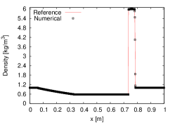
(a) Density

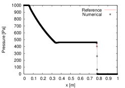
(b) Pressure

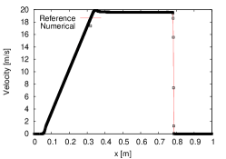
(c) Velocity

Figure 6: Gas-gas Riemann problem.

We carry out the simulation to a final time of 0.012. Fig. 6 shows the comparison between numerical results and exact solutions. From the comparison we can see that the numerical results behave in perfect agreement with the exact solutions.

5.1.2 JWL-polynomial Riemann problem

This example concerns the JWL-polynomial Riemann problem. The initial states are

$$[\rho,u,p]^{\top}=\left\{\begin{array}[]{ll}[1630,~{}0,~{}8.3\times 10^{9}]^{\top},&x<0.5,\\[5.69054pt] [1000,~{}0,~{}1.0\times 10^{5}]^{\top},&x>0.5.\end{array}\right.$$

We use the following values to describe the TNT [61]: $A_{1}=3.712\times 10^{11}\,\mathrm{Pa}$, $A_{2}=3.230\times 10^{9}\,\mathrm{Pa}$, $\omega=0.30$, $R_{1}=4.15$, $R_{2}=0.95$ and $\rho_{0}=1630\,\mathrm{kg/m^{3}}$. The parameters of the polynomial EOS are $\rho_{0}=1000\,\mathrm{kg/m^{3}}$, $A_{1}=2.20\times 10^{9}\,\mathrm{Pa}$, $A_{2}=9.54\times 10^{9}\,\mathrm{Pa}$, $A_{3}=1.45\times 10^{10}\,\mathrm{Pa}$, $B_{0}=B_{1}=0.28$, $T_{1}=2.20\times 10^{9}\,\mathrm{Pa}$ and $T_{2}=0$ [62].

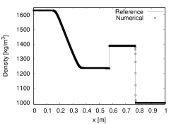
(a) Density

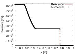
(b) Pressure

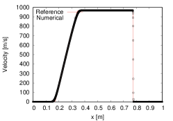
(c) Velocity

Figure 7: JWL-polynomial Riemann problem.

The result at $t=8.0\times 10^{-5}$ is shown in Fig. 7, where we can observe that both the interface and shock are captured well without spurious oscillation.

5.1.3 Gavrilyuk’s elastic solid Riemann problem

In this problem, we simulate an elastic solid Riemann problem [50]. The hydrostatic pressure of the solid is described by the stiffened gas EOS with parameters $\gamma=4.4$, $p_{\infty}=6\times 10^{6}$ Pa. And the deviatoric component obeys the Hooke’s law, whose elastic shear modulus is $\mu^{{}_{\mathscr{E}}}=10^{10}$ Pa. The initial values are given by

$$[\rho,u,p]^{\top}=\left\{\begin{array}[]{ll}[10^{3},~{}100,~{}10^{5}]^{\top},&x<0.5,\\[5.69054pt] [10^{3},~{}-100,~{}10^{5}]^{\top},&x>0.5.\end{array}\right.$$

The comparison between our numerical results and reference solutions at $6.1\times 10^{-5}$ is shown in Fig. 8, from which we can see that our results agree well with the reference solutions, and there is no oscillation in the vicinity of phase interface and shock waves.

(a)

(b)

(c)

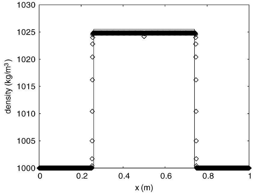
(a) Density

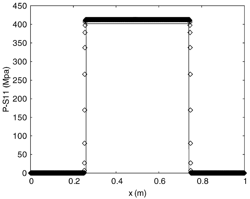
(b) Pressure

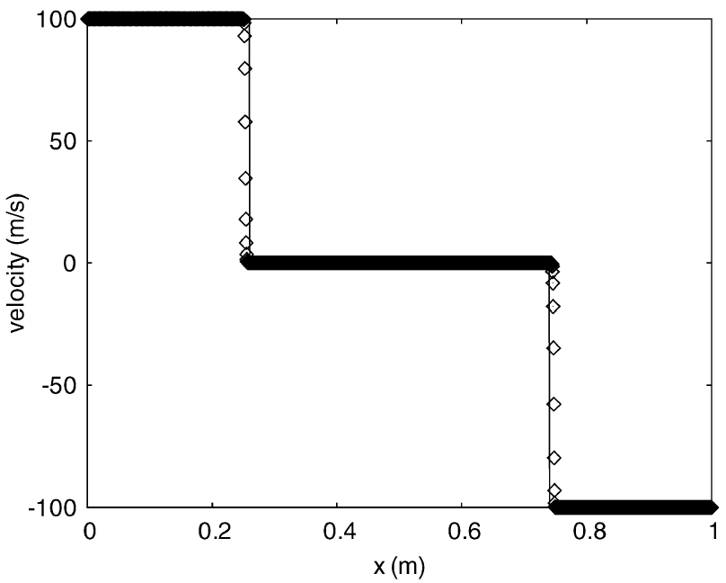
(c) Velocity

Figure 8: Gavrilyuk’s elastic solid Riemann problem (top row: our results, bottom row: results from Gavrilyuk et al. [50]).

5.1.4 JWL-elastic solid Riemann problem

In this problem, we simulate a JWL-elastic solid Riemann problem. The JWL EOS has the following parameter: $A_{1}=8.545\times 10^{11}\,\mathrm{Pa}$, $A_{2}=2.050\times 10^{10}\,\mathrm{Pa}$, $\omega=0.25$, $R_{1}=4.6$, $R_{2}=1.35$, $\rho_{0}=1840\,\mathrm{kg/m^{3}}$. The elastic solid has the same constitutive law as Section 5.1.3 with $\beta^{{}_{\mathscr{E}}}=10^{14}~{}\mbox{Pa}\cdot\mbox{kg/m}^{3}$. The initial values are

$$[\rho,u,p]^{\top}=\left\{\begin{array}[]{ll}[1630,~{}0,~{}9.2\times 10^{9}]^{\top},&x<0.5,\\[5.69054pt] [7800,~{}0,~{}10^{5}]^{\top},&x>0.5.\end{array}\right.$$

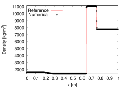
(a) Density

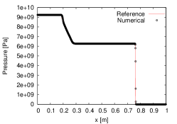
(b) Pressure

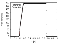
(c) Velocity

Figure 9: JWL-elastic solid Riemann problem.

The computation terminates at $10^{-4}$. Fig. 9 displays the results of our numerical scheme and the exact solutions, where we can see that there is no non-physical pressure and velocity across the contact discontinuity in our numerical scheme.

5.1.5 Perfectly elastoplastic solid Riemann problem

In this problem, we extend our methods to simulate the perfectly elastoplastic solid-solid Riemann problem [45]. We take the Murnagham EOS (23) to describe the hydrostatic pressure of the solid, and set the following parameters for the solid: $\mu^{{}_{\mathscr{E}}}=8.53\times 10^{5}\,\mathrm{Pa},~{}\mu^{{}_{\mathscr{P}}}=0,~{}K=2.225\times 10^{6}\,\mathrm{Pa},~{}Y^{{}_{\mathscr{E}}}=6.50\times 10^{3}\,\mathrm{Pa}$, $Y^{{}_{\mathscr{P}}}=0$. The initial values are given by

$$[\rho,u,p]^{\top}=\left\{\begin{array}[]{ll}[7.8,~{}10,~{}1.0]^{\top},&x<0.5,\\[5.69054pt] [7.8,~{}-5,~{}1.0]^{\top},&x>0.5.\end{array}\right.$$

The comparison between our numerical results and reference solutions at $6.751\times 10^{-4}$ is shown in Fig. 10. Each solid has two nonlinear waves, the leading elastic shock wave and tailing plastic shock wave, and there is no oscillation in the vicinity of phase interface and shock waves. Both the elastic and plastic shock waves are captured correctly.

(a)

(b)

(c)

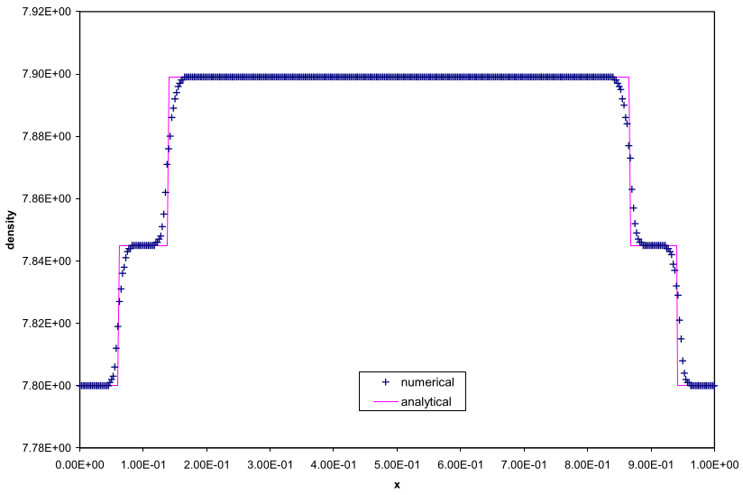
(a) Density

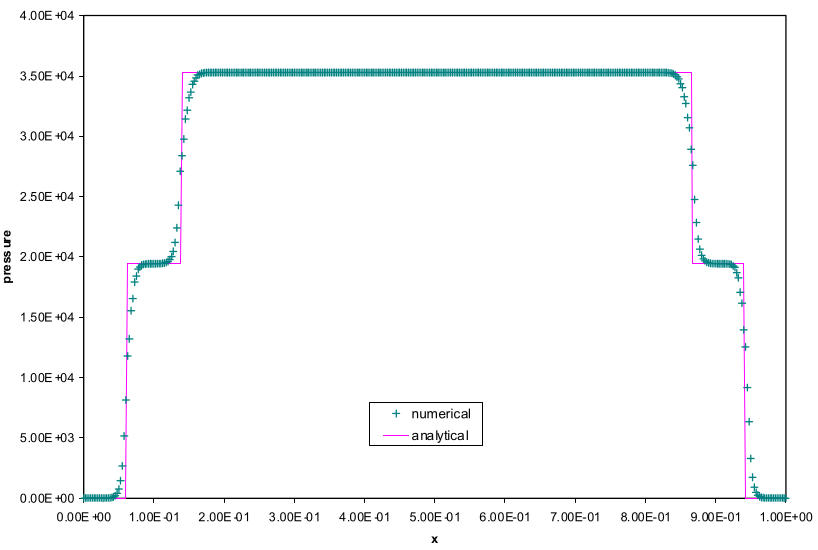
(b) Pressure

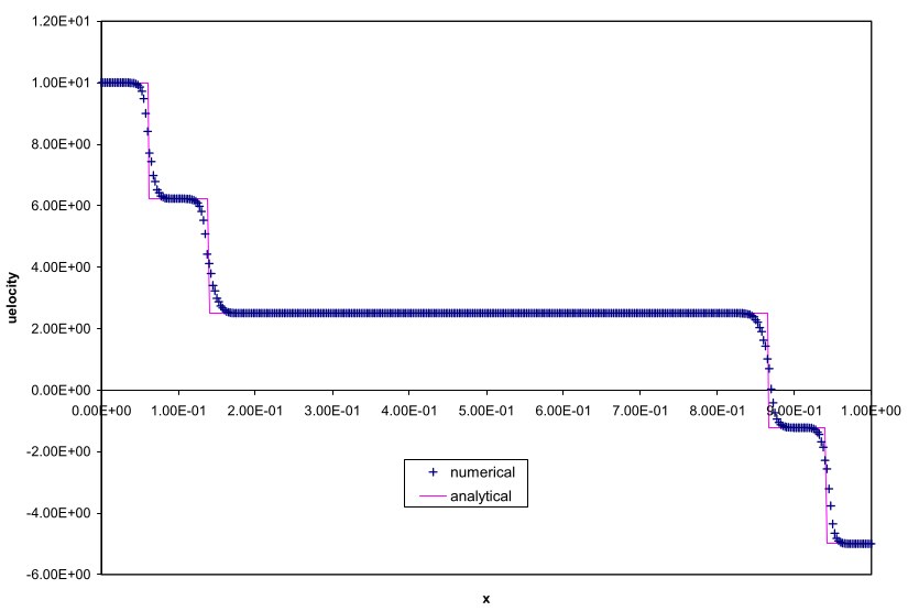
(c) Velocity

Figure 10: Perfectly elastoplastic solid Riemann problem (top panel: our numerical results, bottom panel: reference solutions from T.G. Liu [45]).

5.1.6 Hydro-elastoplastic solid Riemann problem

In this problem, we extend our methods to simulate the hydro-elastoplastic solid Riemann problem [45], which has the same initial conditions and parameters as Section 5.1.5 except $Y^{{}_{\mathscr{P}}}=9.75\times 10^{3}\,\mathrm{Pa}$, $\mu^{{}_{\mathscr{P}}}=\mu^{{}_{\mathscr{E}}}/2$.

Our numerical results at $6.751\times 10^{-4}$ is shown in Fig. 11. Due to the discrepency of the deviatoric constitutive law, each solid has three nonlinear waves, a leading elastic shock wave, an intermediate plastic shock wave and a tailing fluid shock wave. From the comparison, we can see that there is no oscillation in the vicinity of phase interface and shock waves.

(a) Density

(b) Pressure

(c) Velocity

Figure 11: Hydro-elastoplastic solid Riemann problem.

5.2 Two-dimensional applications

In this part, we present a few two-dimensional problems in engineering applications, which are carried out on triangular meshes, including gas-bubble interaction, blast wave reflection, implosion compression and high speed impact problems.

5.2.1 Gas-bubble interaction problem

In this problem, we simulate a gas-bubble interaction problem from Hass [63, 64, 65], which has been widely used as a benchmark problem for validations of numerical schemes. The computational domain for our simulation is shown in Fig. 12. A cylindrical bubble with diameter 50mm is placed in the middle of the square shock tube filled with air. A planar weak shock of Mach number 1.22 vertical to the walls of the shock tube is produced on the right of the bubble, and it propagates towards and hits the bubble. The behaviors of the helium bubble and air are modeled by the ideal gas EOS, and the initial parameters are presented in Tab. 3. The reflective wall boundary conditions are presented on the top and bottom, and outflow conditions are prescribed on the left and right ends of the domain.

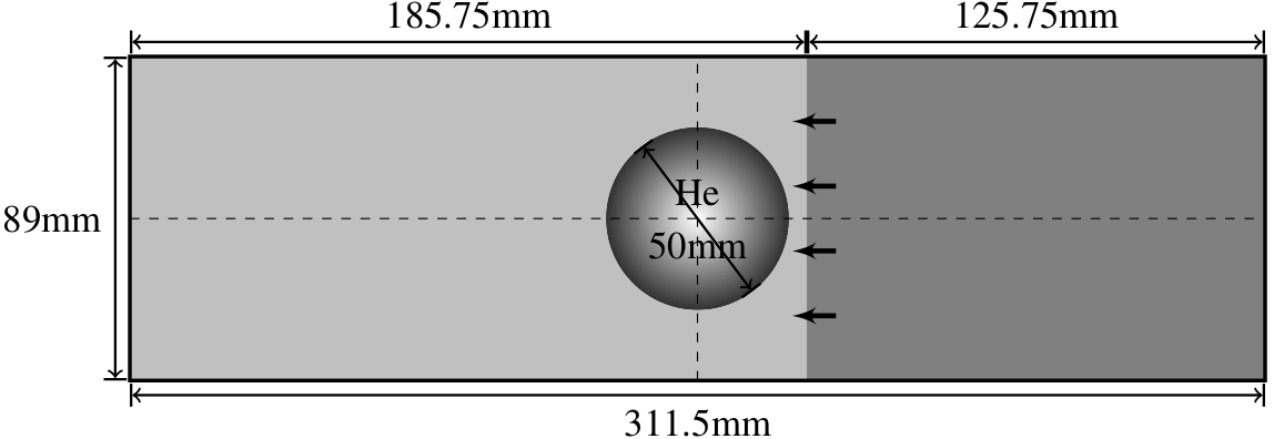
Figure 12: Model of gas-bubble interaction problem.

Table 3: Initial parameters for gas-bubble problem.

Parameters	$\rho(\mbox{kg/m}^{3})$	$u(\mbox{m/s})$	$p(\mbox{Pa})$	$\gamma$
Helium(bubble)	0.2228	0	101325	1.648
Air(Before Shock)	1.2250	0	101325	1.400
Air(After Shock)	1.6861	-113.534	159059	1.400

We present the contour images of the numerical density at the times 23 $\mu$s, 43 $\mu$s, 53 $\mu$s, 66 $\mu$s, 75 $\mu$s, 102 $\mu$s, 260 $\mu$s, 445 $\mu$s, 674 $\mu$s and 983 $\mu$s, and compare them with the experimental shadowgraphs picked from [63] at times 32 $\mu$s, 53 $\mu$s, 62 $\mu$s, 72 $\mu$s, 82 $\mu$s, 102 $\mu$s, 245 $\mu$s, 427 $\mu$s, 674 $\mu$s and 983 $\mu$s. As is seen from the comparison, our numerical results are qualitatively in good agreement with the experiment. Our numerical simulation provides clear images for the severely deformed bubble, especially from 427 $\mu$s to 983 $\mu$s, which show the ability of our methods in dealing with the large deformation of phase interface.

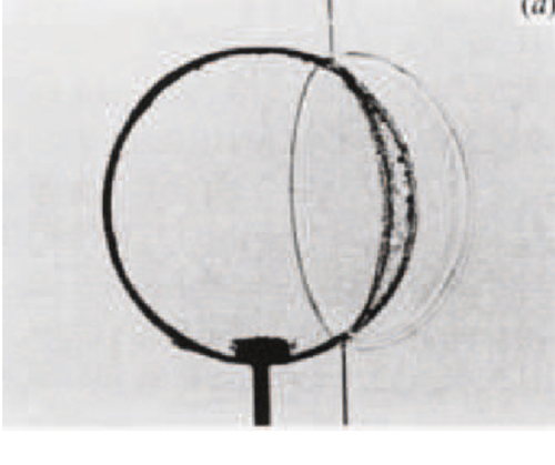
(a)

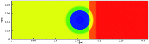
(b)

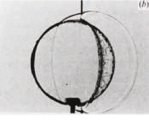
(c)

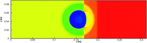
(d)

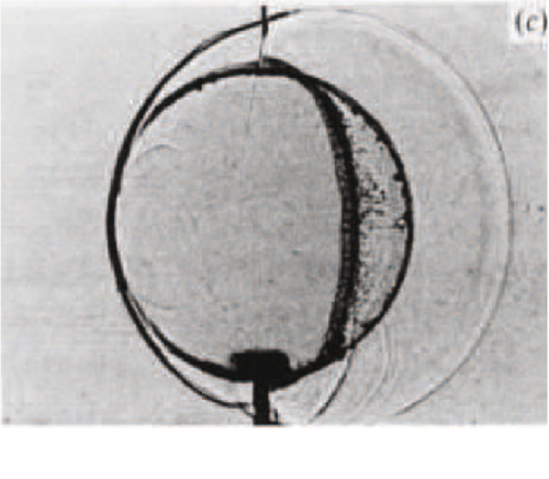
(e)

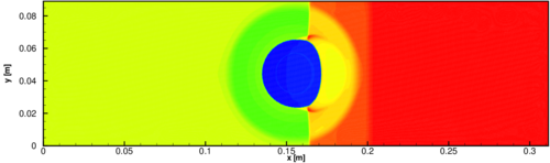
(f)

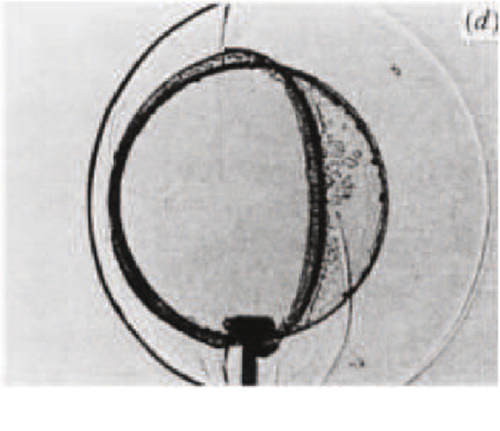
(g)

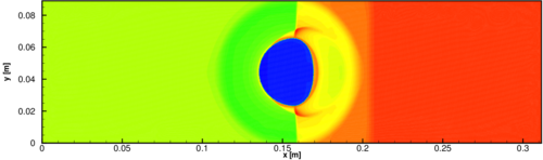
(h)

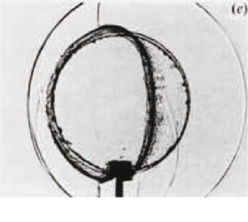
(i)

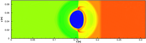
(j)

Figure 13: Gas-bubble interaction problem. The first row: 32$\mu\mbox{s}$, 53$\mu\mbox{s}$, 62$\mu\mbox{s}$, 72$\mu\mbox{s}$, 82$\mu\mbox{s}$;  The second row: 23$\mu\mbox{s}$, 43$\mu\mbox{s}$, 53$\mu\mbox{s}$, 66$\mu\mbox{s}$, 75$\mu\mbox{s}$.

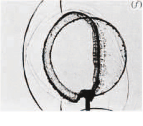
(a)

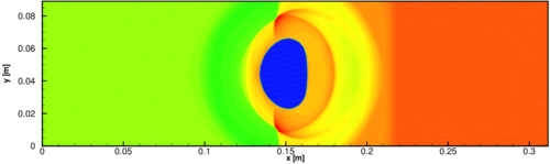
(b)

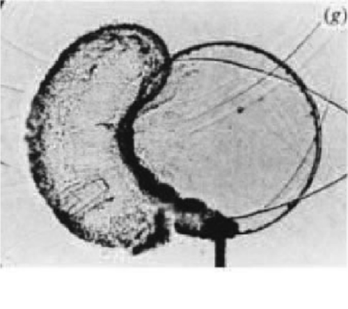
(c)

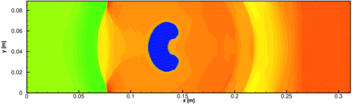
(d)

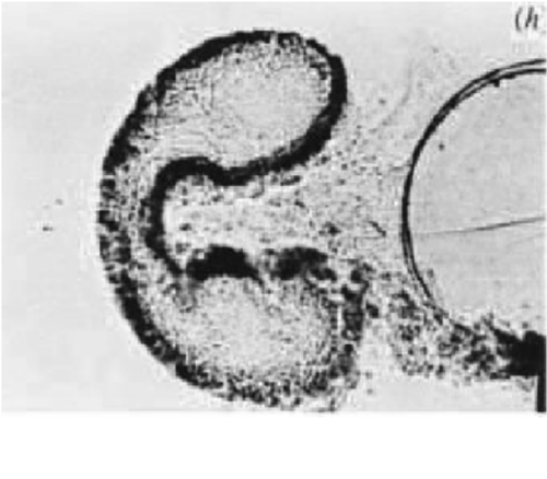
(e)

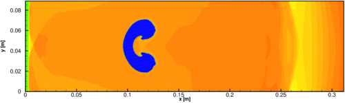
(f)

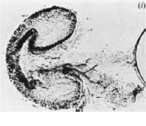
(g)

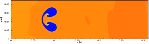
(h)

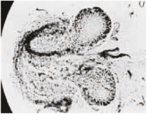
(i)

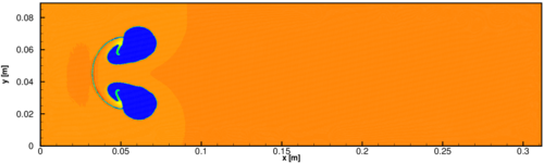
(j)

Figure 14: Gas-bubble interaction problem. The first row: 102$\mu\mbox{s}$, 245$\mu\mbox{s}$, 427$\mu\mbox{s}$, 674$\mu\mbox{s}$, 983$\mu\mbox{s}$;  The second row: 102$\mu\mbox{s}$, 260$\mu\mbox{s}$, 445$\mu\mbox{s}$, 674$\mu\mbox{s}$, 983$\mu\mbox{s}$.

5.2.2 Blast wave reflection of TNT explosion

In this problem, we simulate a TNT explosion problem, where the blast wave is reflected by a rigid surface near the explosion center. We use this example to assess the isotropic behavior of TNT explosion in a computational domain $0\leq r\leq 1\,\mathrm{m},~{}2\,\mathrm{m}\leq z\leq 8\,\mathrm{m}$. The air is modeled by the ideal gas EOS with adiabatic exponent $\gamma=1.4$, and the TNT is modeled by the JWL EOS with the same parameters as Section 5.1.2. The initial conditions are: $\rho=1630\,\mathrm{kg/m^{3}}$, $u=0\,\mathrm{m/s}$, $p=9.5\times 10^{9}\,\mathrm{Pa}$ for the TNT, and $\rho=1.29\,\mathrm{kg/m^{3}}$, $u=0\,\mathrm{m/s}$, $p=1.013\times 10^{5}\,\mathrm{Pa}$ for the air. The initial interface is a sphere of radius $0.0527\,\mathrm{m}$ centered at the height $z=5\,\mathrm{m}$. All of the physical boundaries are set as rigid walls.

The results of shock produced by the high explosives are shown in Fig. 16. From here we can see that the shock wave propagates as an expansive spherical surface in the earlier period. When the spherical shock wave impinges on the rigid surface, it will be reflected firstly and propagate along the rigid wall simultaneously. When the incident angle exceeds the limit, the reflective wave switches from regular to irregular, and a Mach blast wave occurs. The shock parameters, shown in Fig. 16, agree well with the experimental data in [66, 67, 68] and [69].

(a) $t=1.0\mu$s

(b) $t=4.3\mu$s

(c) $t=3.0\mu$s

(d) $t=7.0\mu$s

(e) $t=11.0\mu$s

Figure 15: Pressure contours for TNT explosion problem.

(a) Peak overpressure

(b) Impulse

Figure 16: Shock wave parameters for TNT explosion problem. The reference solution 1 is taken from [66], the reference solution 2 is taken from [67], the reference solution 3 is taken from [68], and the experiment solution is taken from [69].

5.2.3 Implosion compression problem

We consider a two dimensional problem of implosion compression, which is applied widely in inertial confinement fusion applications [70, 71]. The initial shape of the model is a sphere containing three distinct mediums, TNT, tungsten and air. The outmost layer is the high explosive products of TNT , which is described by the JWL EOS with parameters $A_{1}=8.524\times 10^{11}\,\mathrm{Pa}$, $A_{2}=1.802\times 10^{10}\,\mathrm{Pa}$, $\omega=0.38$, $R_{1}=4.6$, $R_{2}=1.3$, $\rho_{0}=1842\,\mathrm{kg/m^{3}}$. The intermediate layer is the tungsten, which is described by the stiffened gas EOS with parameters $\gamma=4.075$, $\rho_{0}=7.85~{}\mbox{g/cm}^{3}$. The innermost layer is the air, which is described by the ideal gas with $\gamma=1.4$. All the boundaries are set as outflow conditions. The initial values are

$$[\rho,u,p]^{\top}=\left\{\begin{array}[]{ll}[1.29,~{}0,~{}10^{5}]^{\top},&r<0.1,\\[5.69054pt] [1.9237\times 10^{4},~{}0,~{}10^{5}]^{\top},&0.1\leq r\leq 0.105,\\[5.69054pt] [1.63\times 10^{3},~{}0,~{}10^{5}]^{\top},&0.105<r<0.12.\\[5.69054pt] \end{array}\right.$$

Fig. 17 and 18 show the pressure contours of the whole computational domain at different time. Due to the high pressure of the explosives at the outmost layer, it produces a strong shock wave inward and drives the tungsten and air moving into the center. The shock wave reaches a smallest radius at $37.5~{}\mu\mbox{s}$, whose pressure will increase to about $1.29\times 10^{12}~{}\mbox{Pa}$. Then the shock wave will expand and propagate outward with a decreasing shock front. The symmetry of shock waves and interfaces are kept well during the whole computation, which shows good efficiency of our schemes dealing with the highly nonlinear equations of state.

(a) $10\times 10^{-6}~{}\mbox{s}$

(b) $20\times 10^{-6}~{}\mbox{s}$

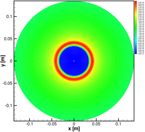
(c) $30\times 10^{-6}~{}\mbox{s}$

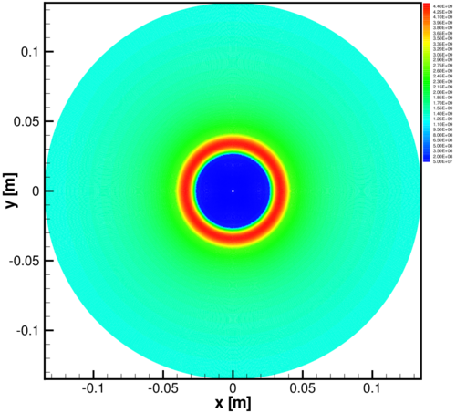
(d) $32\times 10^{-6}~{}\mbox{s}$

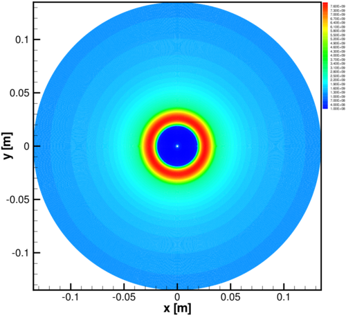
(e) $34\times 10^{-6}~{}\mbox{s}$

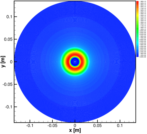
(f) $36\times 10^{-6}~{}\mbox{s}$

Figure 17: Pressure contours for implosion compression problems.

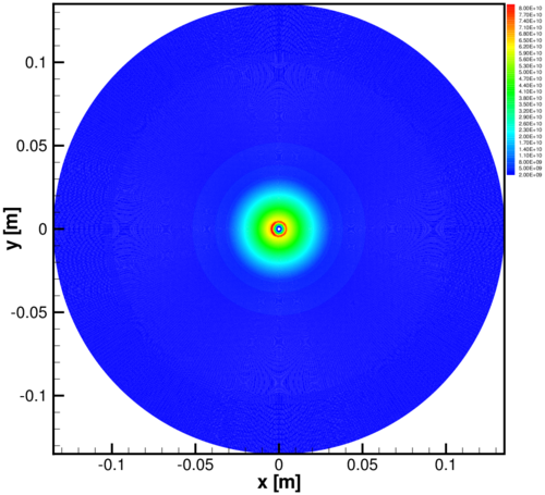
(a) $37\times 10^{-6}~{}\mbox{s}$

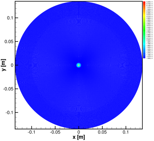
(b) $37.2\times 10^{-6}~{}\mbox{s}$

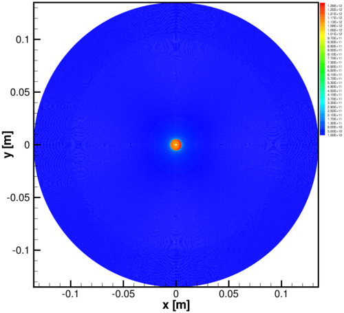
(c) $37.5\times 10^{-6}~{}\mbox{s}$

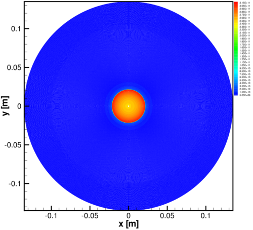
(d) $39\times 10^{-6}~{}\mbox{s}$

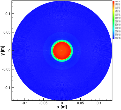
(e) $40\times 10^{-6}~{}\mbox{s}$

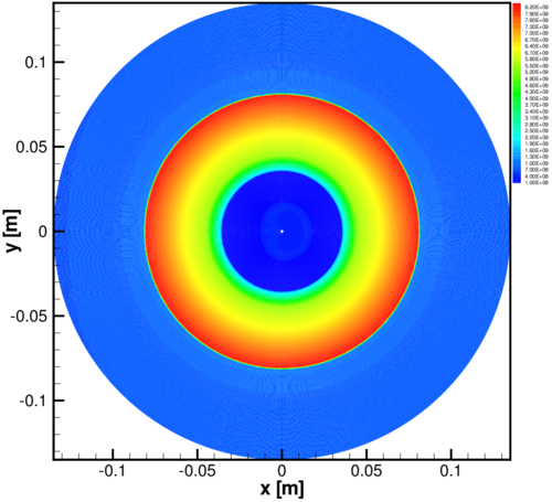
(f) $50\times 10^{-6}~{}\mbox{s}$

Figure 18: Pressure contours for implosion compression problems.

5.2.4 High speed impact applications

In this problem, we simulate a two dimensional high speed impact problem between three elastoplastic solids. A cylindrical rod made of steel with an initial radius of $0.2\,\mathrm{m}$ is given a velocity of $7000\,\mathrm{m/s}$ and impacts against two layers of static aluminum, shown as Fig. 19 (a). Each aluminum has an initial radius of $0.5\,\mathrm{m}$ and a length of $0.2\,\mathrm{m}$. In fact, the whole problem involves three mediums, the steel, the aluminum and the air. The equations of state for the hydrostatic pressure component of the steel and aluminum are both taken as the stiffened gas EOS, and the deviatoric component are both taken as the perfect elastoplasticity. The initial parameters are $\rho_{0}=7840\,\mathrm{kg/m^{3}}$, $\gamma=4.075$, $\mu^{{}_{\mathscr{E}}}=78.5\times 10^{9}\,\mathrm{Pa}$, $\mu^{{}_{\mathscr{P}}}=0$, $Y^{{}_{\mathscr{E}}}=160\times 10^{6}\,\mathrm{Pa}$ for the steel, and $\rho_{0}=2790\,\mathrm{kg/m^{3}}$, $\gamma=2.75$, $\mu^{{}_{\mathscr{E}}}=27.4\times 10^{9}\,\mathrm{Pa}$, $\mu^{{}_{\mathscr{P}}}=0$, $Y^{{}_{\mathscr{E}}}=34\times 10^{6}\,\mathrm{Pa}$ for the aluminum. The air is modeled by the ideal gas EOS with the following initial parameters: $\rho_{0}=1.29\,\mathrm{kg/m^{3}}$, $\gamma=1.4$ and $p_{0}=1.013\times 10^{5}\,\mathrm{Pa}$.

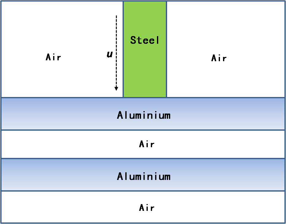
(a) Illustration of the impact model

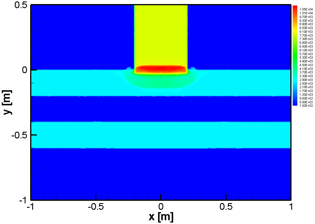
(b) $2.0\times 10^{-7}~{}\mbox{s}$

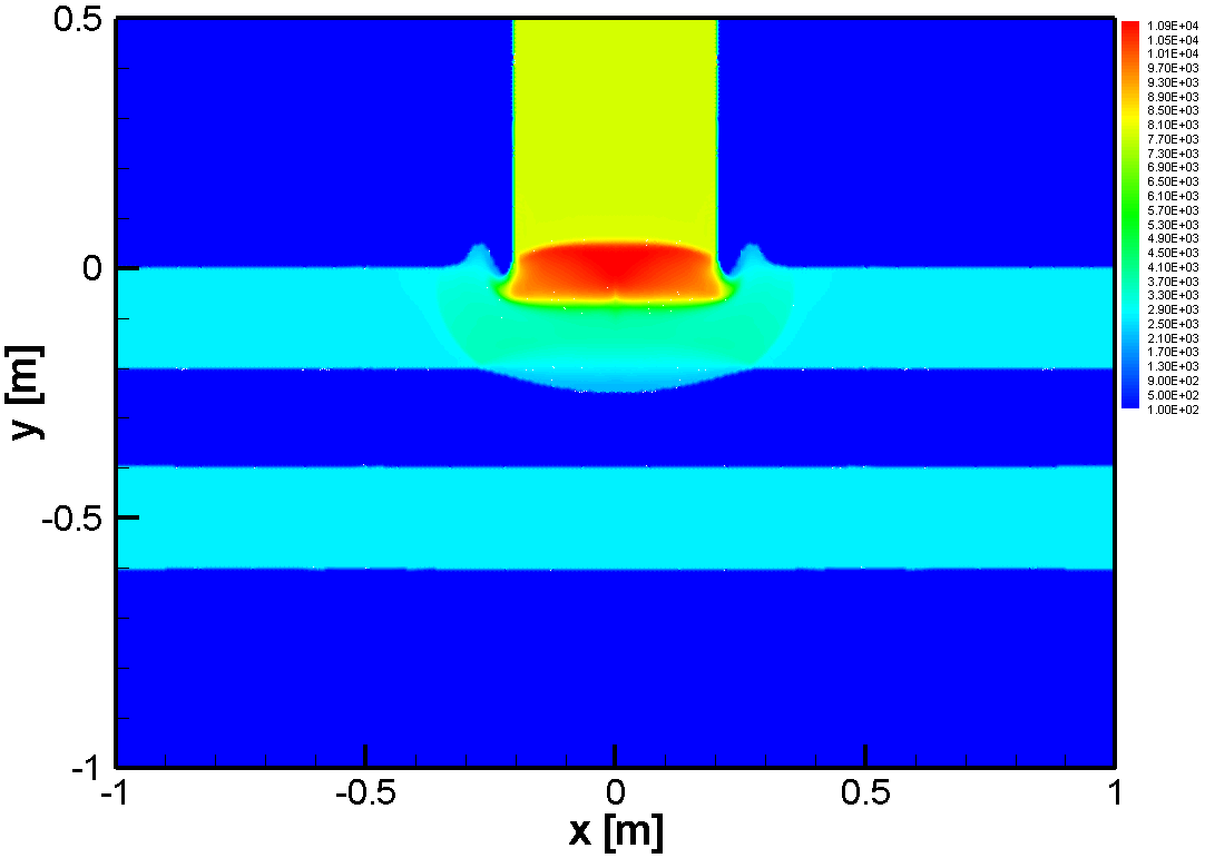
(c) $1.0\times 10^{-6}~{}\mbox{s}$

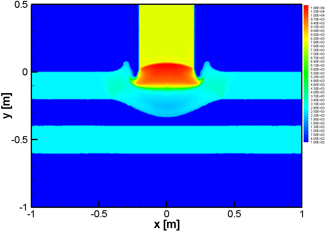
(d) $1.8\times 10^{-6}~{}\mbox{s}$

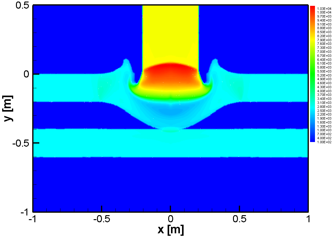
(e) $2.5\times 10^{-6}~{}\mbox{s}$

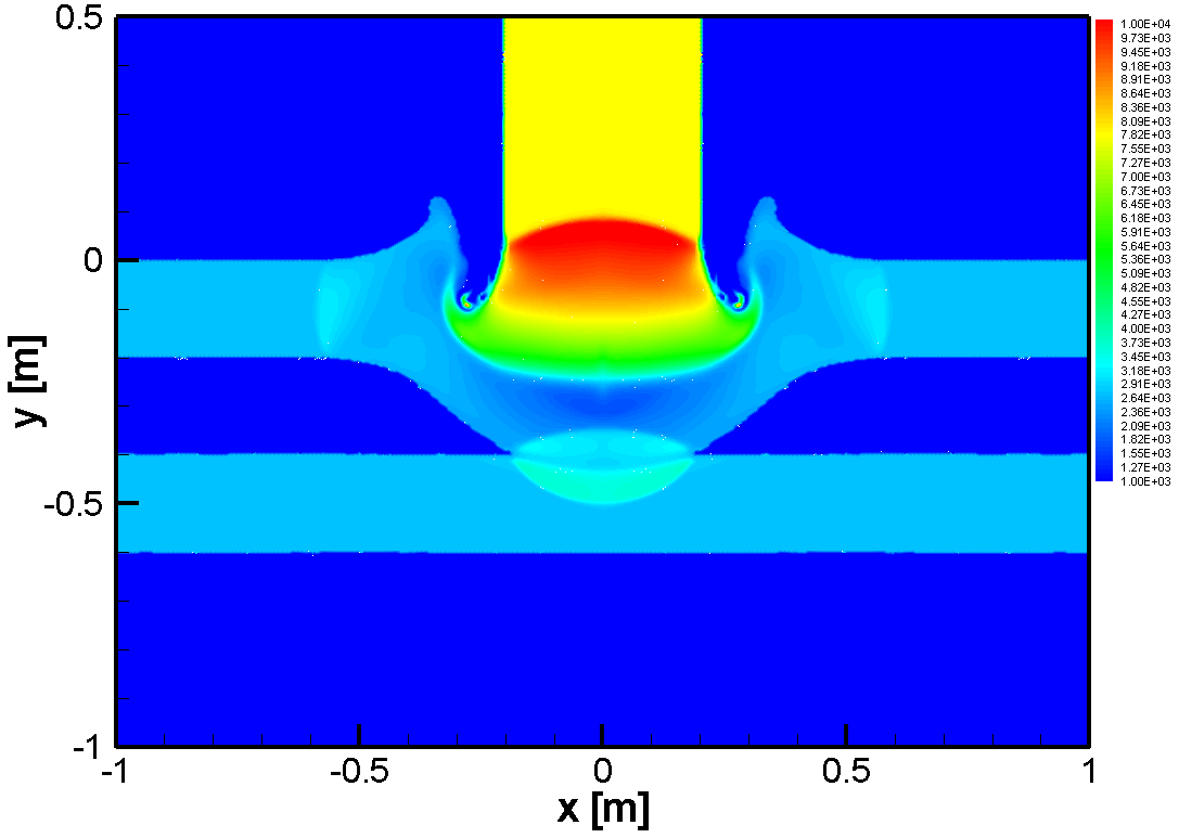
(f) $3.6\times 10^{-6}~{}\mbox{s}$

Figure 19: Density contours for high speed impact problems.

Fig. 19 (b)–(f) show the density contours of the whole steel and aluminum at different time. When the steel rod reaches the aluminum, strong interaction occurs between them. Since the steel has a much higher density and stiffness, it will lead to the severe deformation and penetration of the aluminum finally. In the whole calculation, we can see that the interfaces between each pair of the aluminum, steel and air can be captured sharply, which show that our numerical scheme can handle the large deformation of compressible materials and phase interfaces naturally.

6 Conclusions

We extend the numerical scheme in Guo et al. [52] to the multi-medium interaction problems that obey a general Mie-Grüneisen equations of state for the volumetric deformation and hydro-elastoplastic constitutive law for the deviatoric deformation. The numerical procedures to solve the multi-medium Riemann problem are elaborated. A variety of preliminary numerical examples and engineering applications validate our methods. In our future work, we will generalize the framework to more complex multiphase problems, such as multiphase flow with chemical reaction, heat radiation, and so on, which have great initial density and pressure discrepencies and more complex physical phenomena.

References

References

• [1] D.J. Benson. Computational methods in Lagrangian and Eulerian hydrocodes. Computer Methods in Applied Mechanics and Engineering, 99(2-3):235–394, 1992.
• [2] G.T. Camacho and M. Ortiz. Adaptive Lagrangian modelling of ballistic penetration of metallic targets. Computer Methods in Applied Mechanics and Engineering, 142(3-4):269–301, 1997.
• [3] G.C. Bessette, E.B. Becker, L.M. Taylor, and D.L. Littlefield. Modeling of impact problems using an h-adaptive, explicit lagrangian finite element method in three dimensions. Computer Methods in Applied Mechanics and Engineering, 192(13-14):1649–1679, 2003.
• [4] H.S. Udaykumar, H.C. Kan, W. Shyy, and R. Tran-Son-Tay. Multiphase dynamics in arbitrary geometries on fixed Cartesian grids. Journal of Computational Physics, 137(2):366–405, 1997.
• [5] L. Tran and H.S. Udaykumar. A particle-level set-based sharp interface Cartesian grid method for impact, penetration, and void collapse. Journal of Computational Physics, 193(2):469–510, 2004.
• [6] H.S. Udaykumar, L. Tran, D.M. Belk, and K.J. Vanden. An Eulerian method for computation of multimaterial impact with ENO shock-capturing and sharp interfaces. Journal of Computational Physics, 186(1):136–177, 2003.
• [7] S.K. Sambasivan and H.S. Udaykumar. A sharp interface method for high-speed multi-material flows: strong shocks and arbitrary materialpairs. International Journal of Computational Fluid Dynamics, 25(3):139–162, 2011.
• [8] S. Sambasivan, A. Kapahi, and H.S. Udaykumar. Simulation of high speed impact, penetration and fragmentation problems on locally refined Cartesian grids. Journal of Computational Physics, 235:334–370, 2013.
• [9] A. Kapahi, S. Sambasivan, and H.S. Udaykumar. A three-dimensional sharp interface cartesian grid method for solving high speed multi-material impact, penetration and fragmentation problems. Journal of Computational Physics, 241:308–332, 2013.
• [10] J.T. Wang, K.X. Liu, and D.L. Zhang. An improved CE/SE scheme for multi-material elastic–plastic flows and its applications. Computers & Fluids, 38(3):544–551, 2009.
• [11] G. Wang, D.L. Zhang, and K.X. Liu. An improved CE/SE scheme and its application to detonation propagation. Chinese Physics Letters, 24(12):3563, 2007.
• [12] G. Wang, D.L. Zhang, K.X. Liu, and J.T. Wang. An improved CE/SE scheme for numerical simulation of gaseous and two-phase detonations. Computers & Fluids, 39(1):168–177, 2010.
• [13] Q.Y. Chen and K.X. Liu. A high-resolution Eulerian method for numerical simulation of shaped charge jet including solid–fluid coexistence and interaction. Computers & Fluids, 56:92–101, 2012.
• [14] Q.Y. Chen, J.T. Wang, and K.X. Liu. Improved CE/SE scheme with particle level set method for numerical simulation of spall fracture due to high-velocity impact. Journal of Computational Physics, 229(19):7503–7519, 2010.
• [15] S. Hua, K.X. Liu, and D.L. Zhang. Three-dimensional simulation of detonation propagation in a rectangular duct by an improved CE/SE scheme. Chinese Physics Letters, 28(12):124705, 2011.
• [16] B. Mehmandoust and A.R. Pishevar. An Eulerian particle level set method for compressible deforming solids with arbitrary EOS. International Journal for Numerical Methods in Engineering, 79(10):1175–1202, 2009.
• [17] C.D. Sijoy and S. Chaturved. An Eulerian multi-material scheme for elastic–plastic impact and penetration problems involving large material deformations. European Journal of Mechanics-B/Fluids, 53:85–100, 2015.
• [18] R. Abgrall. How to prevent pressure oscillations in multicomponent flow calculations: a quasi conservative approach. Journal of Computational Physics, 125(1):150–160, 1996.
• [19] R. Abgrall and S. Karni. Computations of compressible multifluids. Journal of Computational Physics, 169(2):594–623, 2001.
• [20] R. Saurel and R. Abgrall. A simple method for compressible multifluid flows. SIAM Journal on Scientific Computing, 21(3):1115–1145, 1999.
• [21] R. Saurel, F. Petitpas, and R.A. Berry. Simple and efficient relaxation methods for interfaces separating compressible fluids, cavitating flows and shocks in multiphase mixtures. Journal of Computational Physics, 228(5):1678–1712, 2009.
• [22] F. Petitpas, J. Massoni, and R. Saurel. Diffuse interface model for high speed cavitating underwater systems. International Journal of Multiphase Flow, 35(8):747–759, 2009.
• [23] M.R. Ansari and A. Daramizadeh. Numerical simulation of compressible two-phase flow using a diffuse interface method. International Journal of Heat and Fluid Flow, 42(8):209–223, 2013.
• [24] R. Scardovelli and S. Zaleski. Direct numerical simulation of free-surface and interfacial flow. Annual Review of Fluid Mechanics, 31(1):567–603, 1999.
• [25] W.F. Noh and P. Woodward. SLIC (simple line interface calculation). In Proceedings of the Fifth International Conference on Numerical Methods in Fluid Dynamics, pages 330–340. Springer, 1976.
• [26] J.A. Sethian. Evolution, implementation, and application of level set and fast marching methods for advancing fronts. Journal of Computational Physics, 169(2):503–555, 2001.
• [27] M. Sussman, P. Smereka, and S. Osher. A level set approach for computing solutions to incompressible two-phase flow. Journal of Computational Physics, 114(1):146–159, 1994.
• [28] H.T. Ahn and M. Shashkov. Multi-material interface reconstruction on generalized polyhedral meshes. Journal of Computational Physics, 226(2):2096–2132, 2007.
• [29] V. Dyadechko and M. Shashkov. Reconstruction of multi-material interfaces from moment data. Journal of Computational Physics, 227(11):5361–5384, 2008.
• [30] H.R. Anbarlooei and K. Mazaheri. Moment of fluid interface reconstruction method in multi-material arbitrary Lagrangian Eulerian (MMALE) algorithms. Computer Methods In Applied Mechanics And Engineering, 198(47):3782–3794, 2009.
• [31] J. Glimm, J.W. Grove, and X.L. Li. Three-dimensional front tracking. SIAM Journal on Scientific Computing, 19(3):1703–727, 1998.
• [32] G. Tryggvason, B. Bunner, and A. Esmaeeli. A front-tracking method for the computations of multiphase flow. Journal of Computational Physics, 169(2):708–759, 2001.
• [33] H.S. Yadav and V.P. Singh. Converging shock waves in metals. Pramana, 18(4):331–338, 1982.
• [34] K.M. Shyue. A fluid-mixture type algorithm for compressible multicomponent flow with Mie–Grüneisen equation of state. Journal of Computational Physics, 171(2):678–707, 2001.
• [35] M. Arienti, E. Morano, and J.E. Shepherd. Shock and detonation modeling with the Mie-Grüneisen equation of state. Technical report, California Institute of Technology, 2004.
• [36] B.J. Lee, E.F. Toro, C.E. Castro, and N.Nikiforakis. Adaptive Osher-type scheme for the Euler equations with highly nonlinear equations of state. Journal of Computational Physics, 246:165–183, 2013.
• [37] J.W. Banks. On exact conservation for the Euler equations with complex equations of state. Communications in Computational Physics, 8(5):995, 2010.
• [38] J.R. Kamm. Solution of the 1D Riemann problem with a general EOS in ExactPack. In 4th ASME Conference on Verification and Validation of Simulations, Las Vegas, NV, 2015.
• [39] A. Kaboudian and B.C. Khoo. The ghost solid method for the elastic solid–solid interface. Journal of Computational Physics, 257:102–125, 2014.
• [40] L. Xiao. Numerical computation of stress waves in solids. Akademie Verlag Gmbh, Berlin, 1996.
• [41] H.S. Tang and F. Sotiropoulos. A second-order Godunov method for wave problems in coupled solid–water–gas systems. Journal of Computational Physics, 151(2):790–815, 1999.
• [42] M. Abouziarov, V.G. Bazhenov, V. Kotov, A.V. Kochetkov, S.V. Krylov, and V.R. Fel’dgun. A Godunov-type method in dynamics of elastoplastic media. Zhurnal Vychislitel’noi Matematiki i Matematicheskoi Fiziki, 40(6):940–953, 2000.
• [43] V.G. Bazhenov and V.L. Kotov. Modification of Godunov’s numerical scheme for solving problems of pulsed loading of soft soils. Journal of Applied Mechanics and Technical Physics, 43(4):603–611, 2002.
• [44] I.S. Menshov, A.V. Mischenko, and A.A. Serejkin. Numerical modeling of elastoplastic flows by the Godunov method on moving Eulerian grids. Mathematical Models and Computer Simulations, 6(2):127–141, 2014.
• [45] T.G. Liu, W.F. Xie, and B.C. Khoo. The modified ghost fluid method for coupling of fluid and structure constituted with hydro-elasto-plastic equation of state. SIAM Journal on Scientific Computing, 30(3):1105–1130, 2008.
• [46] T.G. Liu, A.W. Chowdhury, and B.C. Khoo. The modified ghost fluid method applied to fluid-elastic structure interaction. Advances in Applied Mathematics and Mechanics, 3(05):611–632, 2011.
• [47] Z.W. Feng, A. Kaboudian, J.L. Rong, and B.C. Khoo. The simulation of compressible multi-fluid multi-solid interactions using the modified ghost method. Computers & Fluids, 2017.
• [48] S. Gao and T.G. Liu. 1D exact elastic-perfectly plastic solid Riemann solver and its multi-material application. Advances in Applied Mathematics and Mechanics, 9(3):621–650, 2017.
• [49] S. Gao, T.G. Liu, and C.B. Yao. A complete list of exact solutions for one-dimensional elastic-perfectly plastic solid Riemann problem without vacuum. Communications in Nonlinear Science and Numerical Simulation, 63(2):205–227, 2018.
• [50] S.L. Gavrilyuk, N. Favrie, and R. Saurel. Modelling wave dynamics of compressible elastic materials. Journal of Computational Physics, 227(5):2941–2969, 2008.
• [51] B. Despres. A geometrical approach to nonconservative shocks and elastoplastic shocks. Archive for Rational Mechanics and Analysis, 186(2):275–308, 2007.
• [52] Y.H. Guo, R. Li, and C.B. Yao. A numerical method on Eulerian grids for two-phase compressible flow. Advances in Applied Mathematics and Mechanics, 8(2):187–212, 2016.
• [53] L. Chen, R. Li, and C.B. Yao. An approximate solver for multi-medium Riemann problem with Mie-Grüneisen equations of state. Research in the Mathematical Sciences, 5(3):31–59, 2018.
• [54] R.S. Dembo, S.C. Eisenstat, and T. Steihaug. Inexact Newton methods. SIAM Journal on Numerical Analysis, 19(2):400–408, 1982.
• [55] O. Heuzé. General form of the Mie–Grüneisen equation of state. Comptes Rendus Mecanique, 340(10):679–687, 2012.
• [56] J.A. Trangenstein and P. Colella. A higher-order Godunov method for modeling finite deformation in elastic-plastic solids. Communications on Pure and Applied Mathematics, 44(1):41–100, 1991.
• [57] S.K. Godunov, A.V. Zabrodin, M.I. Ivanov, A.N. Kraiko, and G.P. Prokopov. Numerical solution of multidimensional problems of gas dynamics. Moscow Izdatel Nauka, 1, 1976.
• [58] E. Fehlberg. Klassische Runge-Kutta-Formeln vierter und niedrigerer Ordnung mit Schrittweiten-Kontrolle und ihre Anwendung auf Wäermeleitungsprobleme. Computing, 6(1-2):61–71, 1970.
• [59] Y. Di, R. Li, T. Tang, and P. Zhang. Level set calculations for incompressible two-phase flows on a dynamically adaptive grid. Journal of Scientific Computing, 31(1):75–98, 2007.
• [60] E.F. Toro. Riemann Solver and Numerical Methods for Fluid Dynamics. Springer, 2008.
• [61] R.W. Smith. AUSM (ALE): a geometrically conservative arbitrary Lagrangian–Eulerian flux splitting scheme. Journal of Computational Physics, 150(1):268–286, 1999.
• [62] N. Jha and B.S.K. Kumar. Under water explosion pressure prediction and validationa using ANSYS/AUTODYN. International Journal of Science and Research, 3:1162–1165, 2014.
• [63] J.F. Haas and B. Sturtevant. Interaction of weak shock waves with cylindrical and spherical gas inhomogeneities. Journal of Fluid Mechanics, 181:41–76, 1987.
• [64] M.A. Ullah, W. Gao, and D. Mao. Towards front-tracking based on conservation in two space dimensions III, tracking interfaces. Journal of Computational Physics, 242:268–303, 2013.
• [65] J.J. Quirk and S. Karni. On the dynamics of a shock–bubble interaction. Journal of Fluid Mechanics, 318:129–163, 1996.
• [66] W.E. Baker. Explosions in Air. University of Texas Press, 1973.
• [67] N.J. Huffington Jr and W.O. Ewing. Reflected impulse near spherical charges. 1985.
• [68] J.C. Hokanson, E.D. Esparza, and A.B. Wenzel. Blast Effects of Simultaneous Multiple-Charge Detonations. 1978.
• [69] D.Z. Zhang, Y. Li, and D.W. Wang. Experiment investigations on normal reflected blast wave near the sperical explosive (in chinese). Acta Armamentarii, 12:1663–1667, 2009.
• [70] J.D. Lindl. Inertial confinement fusion: the quest for ignition and energy gain using indirect drive. American Institute of Physics, 1998.
• [71] Z.P. Jia, H.D. Zhang, and X.J. Yu. Numerical Methods of Multi-material Simulations. Peking: Science Press, 2014.
• [72] A.S.D. Rallu. A Multiphase Fluid-Structure Computational Framework for Underwater Implosion Problems. PhD thesis, Stanford University, 2009.
• [73] C. Wang, H. Tang, and T. Liu. An adaptive ghost fluid finite volume method for compressible gas–water simulations. Journal of Computational Physics, 227(12):6385–6409, 2008.
• [74] N.N. Autodyn. Autodyn Theory Manual, 2003.