Seismic characterization of multiple fracture sets at Rulison Field, Colorado

Abstract

Conventional fracture-characterization methods assume the presence of a single set of aligned, vertical cracks in the subsurface. We relax this assumption and demonstrate the feasibility of seismic characterization of multiple fracture sets. Our technique relies on recent numerical findings, indicating that multiple, differently oriented, possibly intersecting planar cracks embedded in an otherwise isotropic host rock result in a nearly orthorhombic (or orthotropic) effective medium. Here, the governing parameters of crack-induced orthotropy are estimated from 3D, wide-azimuth, multicomponent seismic reflection data acquired over the tight-gas Rulison Field in Colorado, USA.

We translate strong azimuthal variations of the normal-moveout velocities into interval crack densities, fracture orientations, type of fluid infill, and velocities of the P- and S-waves in an unfractured rock. Our inversion procedure identifies a set of cracks aligned in approximately WNW-ESE direction in the western part of the study area and multiple, likely intersecting fractures in its eastern part. We validate both our underlying theoretical model and the obtained estimates by two independent measurements: (i) the estimated fluid-infill parameter indicates dry cracks as expected for the gas-producing sandstones at Rulison; and (ii) the obtained crack orientations are supported by measurements in a well. As a by-product of fracture characterization, we build an anisotropic velocity model of the Rulison reservoir that, we believe, is the first orthorhombic velocity field constructed from surface seismic data.

I Introduction

Naturally fractured rocks are widely recognized as potential hydrocarbon-bearing formations. Perhaps this is why the 2004 Summer Research Workshop of the Society of Exploration Geophysics (SEG) and the European Association of Geoscientists and Engineers (EAGE) was held to determine the state of the art of seismic characterization of fractured reservoirs. The workshop demonstrated that current industry capabilities of inverting parameters of small, sub-seismic fractures are limited to a single set of penny-shaped, vertical cracks embedded in an otherwise isotropic host rock. This arrangement leads to the effective horizontal transverse isotropy (HTI), its anisotropy coefficients can be estimated from seismic data and related back to the fractures. The papers presented at the workshop exploited HTI model and discussed various approaches to inferring the crack density, fracture orientation, and the type of fluid infill from such seismic signatures as normal-moveout (NMO) velocitiesBerthetetal2004 , amplitude-versus-offset (AVO) variationsdelMonteetal2004 ; GrayTodorovic2004 ; Minsleyetal2004 ; Todorovicetal2004 , and shear-wave splitting coefficientsGaiserVanDok2004 .

As all of the above mentioned techniques are inherently based on measuring the magnitude of azimuthal anisotropy in a selected seismic signature and translating it into the parameters of a single set of cracks, they are bound to produce misleading results in the presence of differently oriented fractures. Such fractures are observed at numerous outcrops throughout the globe and usually identified in the borehole televiewer dataLaubachetal2004 . Given the ubiquity of multiple fracturing, the inadequacy of existing fracture-characterization technology might be explained by an inherent nonuniqueness in inverting the effective anisotropy (estimated from seismic data) for the parameters associated with multiple crack systems. Indeed, the number of fracture-related parameters can be arbitrarily large, whereas the maximum number of independent effective stiffness coefficients for any homogeneous rock volume is 21. While the number 21 obviously imposes an ultimate limit on the number $N$ of fracture sets that can be uniquely resolved from long-wavelength seismic data, this $N$ is typically greater than one. Grechka and TsvankinGrechkaTsvankin2003 used the linear slip theorySchoenberg1980 to derive limits for $N$. They found, in agreement with earlier resultsBakulinetalPart22000 , that seismic data can uniquely constrain the parameters of up to two vertical, rotationally-invariant fracture sets embedded in isotropic background rock.

To make further progress in fracture characterization, one has to rely on certain microstructural information related to the cracks. Such information was utilized in the effective media theory proposed by KachanovKachanov1980 . Being similar to the popular linear slip theorySchoenberg1980 for dry cracks, Kachanov’s theory adds the following important insight: the collective contribution of multiple sets of dry fractures to the effective elasticity is largely controlled by a symmetric, second-rank crack-density tensor; such fractures are sometimes termed scalarSchoenbergSayers1995 . The ability of representing multiple crack systems in an otherwise isotropic rock by a second-rank tensor leads to orthorhombic effective symmetry for any orientations of multiple fracture sets, implying that arbitrarily oriented, vertical cracks can be replaced by two mutually orthogonal sets, called the principal sets, as far as propagation of long seismic waves is concerned. (Here and throughout the paper, the term “long” refers to waves whose lengths are orders of magnitude greater than the crack sizes.) The effective orthotropy induced by dry cracks residing in a purely isotropic host rock turns out to be remarkably simple: it is fully described by only four independent quantities instead of nine needed for general orthotropy. These quantities are the two principal crack densities and two Lamé constants of the isotropic background.

Those findingsKachanov1980 ; Kachanov1993 are extremely valuable for fracture characterization because they reduce any number of vertical fracture sets to just two and, thus, provide a theoretical basis for estimating parameters of multiple systems of fractures. Prior to using these theoretical predictions for parameter estimation, however, it is important to establish their accuracy and the range of validity. This work has been carried out in a series of papersGrechkaKachanovORTfrac2006 ; GrechkaKachanovXfrac2006 ; GrechkaetalSfrac2006 . Their authors performed finite element simulations of effective elasticity for a wide variety of crack arrays that contained planar, open and partially closed, intersecting and non-intersecting, circular and irregular dry fractures. The resultsGrechkaKachanovORTfrac2006 ; GrechkaKachanovXfrac2006 ; GrechkaetalSfrac2006 demonstrate that deviations from effective orthotropy do not exceed 2% in the entire range of the crack densities expected in naturally fractured formations. Moreover, the effective orthotropy holds for liquid-filled cracks even with a better accuracy than for dry cracks because of the stiffening of fractures by fluids and a subsequent reduction of crack contribution to the overall elasticityGrechkaKachanovORTfrac2006 . Following numerical verification of the effective crack-induced orthotropy, a technique for characterization of multiple vertical fracture sets was proposedGrechkaKachanovORTfrac2006 . While being similar to an earlier suggested methodBakulinetalPart22000 , the former does not require information about the vertical velocities. It utilizes only multiazimuth, multicomponent seismic reflection data to estimate the orientations and crack densities of two principal fracture sets, the density-normalized Lamé constants of the background, and the so-called fluid factor that varies from 0 (when the cracks are dry) to 1 (when the bulk modulus of the infill approaches that of the background).

Here we apply this fracture-characterization technique to a 3D, 9C, wide-azimuth data set acquired by the Reservoir Characterization Project (Colorado School of Mines) over the tight-gas Rulison Field located in Colorado, USA. We invert the interval NMO ellipses of the P, S₁ (fast shear), and S₂ (slow shear) waves for the two principal crack densities, fracture azimuths, and fluid factors. The fracture orientations obtained from seismic are supported by direct borehole measurements, whereas the fluid factors turn out to be less than 0.01, as expected for the gas-bearing sandstones at the Rulison. Overall, we find the model of crack-induced orthotropy to adequately explain our data and allow us to characterize multiple fracture sets.

II Theoretical background

II.1 Effective anisotropy induced by vertical cracks

The effective compliance tensor, $\bm{s}_{e}$, of a fractured isotropic rock is generally represented as the sum,

$$\bm{s}_{e}=\bm{s}_{b}+\Delta\bm{s}\,,$$ (1)

of the compliance, $\bm{s}_{b}$, of the unfractured background and the cumulative contribution, $\Delta\bm{s}$, of multiple fractures. In the non-interaction approximationKachanov1980 ; Kachanov1993 ; GrechkaKachanovORTfrac2006 , the nonzero elements of tensor $\Delta\bm{s}$ (in Voigt notation) are

$$\Delta s_{11} =\frac{16\,{e}_{1}\,(1-\nu_{b}^{2})}{3\,E_{b}}\,(1-\varsigma)\,,\quad\Delta s_{55}=\frac{32\,{e}_{1}\,(1-\nu_{b}^{2})}{3\,E_{b}\,(2-\nu_{b})}\,,$$

$$\Delta s_{22} =\frac{16\,{e}_{2}\,(1-\nu_{b}^{2})}{3\,E_{b}}\,(1-\varsigma)\,,\quad\Delta s_{44}=\frac{32\,{e}_{2}\,(1-\nu_{b}^{2})}{3\,E_{b}\,(2-\nu_{b})}\,,$$ (2)

$$\Delta s_{66} =\Delta s_{44}+\Delta s_{55}\,.$$

Here ${e}_{1}$ and ${e}_{2}$ are the densities of the two principal vertical fracture sets, $0\leq\varsigma\leq 1$ is the fluid factor ($\varsigma\approx 0$ for dry cracks, $\varsigma\approx 1$ for liquid-filled ones), and $E_{b}$ and $\nu_{b}$ are the Young’s modulus and Poisson’s ratio of the background, respectively. They are given by the standard expressions,

$$E_{b}=\mu_{b}\,\frac{3\,\lambda_{b}+2\,\mu_{b}}{\lambda_{b}+\mu_{b}}~{}~{}\text{and}~{}~{}\nu_{b}=\frac{\lambda_{b}}{2\,(\lambda_{b}+\mu_{b})}\,,$$ (3)

in terms of the Lamé parameters $\lambda_{b}$ and $\mu_{b}$ of the host rock. The compliance components in equations II.1 are written in the coordinate frame whose ${x}_{1}$ and ${x}_{2}$ axes are normal to the two principal fracture sets, and the ${x}_{3}$ axis is vertical.

The predictions of the non-interaction effective media theory (equations 1 and II.1) appear to be remarkably simple. Yet, their high accuracy has been confirmed numerically for fracture arrays that grossly violate the assumptions of the non-interaction approximationGrechkaKachanovORTfrac2006 ; GrechkaKachanovXfrac2006 ; GrechkaetalSfrac2006 . Specifically, formulations 1 and II.1 remain sufficiently accurate for multiple sets of differently oriented, irregularly shaped, partially closed cracks that might intersect each other and form interconnected fracture networks. This means that long (compared to the crack sizes) seismic waves propagating through those fractures “see” them as if they were isolated and orthogonal to each other. As a result, the effective symmetry sensed by such long seismic waves is nearly orthorhombic even though no local symmetry exists on the scale of a few fractures. This conclusion leads to devising an efficient scheme for inverting the fracture parameters from seismic data.

II.2 Inversion strategy

As follows from equations 1 – 3, the effective elastic properties of rocks with multiple vertical fracture sets are described by the parameter vector

$$\bm{m}=\big{\{}\lambda_{b},\,\mu_{b},\,{e}_{1},\,{e}_{2},\,\varsigma\big{\}}\,$$ (4)

that might vary spatially on the scale of seismic survey. Grechka and KachanovGrechkaKachanovORTfrac2006 demonstrated that all components of $\bm{m}$ can be uniquely estimated from 3D, multiazimuth, multicomponent seismic reflection data. (Of course, seismic data constrain the density-normalized background Lamé constants rather than $\lambda_{b}$ and $\mu_{b}$ themselves.) In particular, it has been shown that $\bm{m}$ can be unambiguously inverted from data

$$\bm{d}(\bm{m})=\left\{\frac{V_{S1}}{V_{P0}},\,\frac{V_{S2}}{V_{P0}},\,\bm{W}^{P},\,\bm{W}^{S1},\,\bm{W}^{S2}\right\},$$ (5)

where $V_{P0}$, $V_{S1}$, and $V_{S2}$ are the velocities of the vertically propagating P- and two split shear-waves (the fast S₁ and the slow S₂). The velocity ratios entering $\bm{d}$ can be computed from the zero-offset times after establishing the P-to-S event correspondence. The $2\times 2$ matrices $\bm{W}$ in equation 5 are the normal-moveout (NMO) ellipses of pure modes reflected from a horizontal interfaceGrechkaTsvankin1998 .

Vertical cracks result in effective orthorhombic media with two vertical symmetry planes, therefore, all three NMO ellipses $\bm{W}^{P}$, $\bm{W}^{S1}$, and $\bm{W}^{S2}$ are always co-oriented for a horizontal reflector, their axes pointing along the normals to the two principal fracture sets. Consequently, data vector $\bm{d}$ given by equation 5 contains eight quantities: two velocity ratios and three pairs of the ellipse semi-axes — the symmetry-direction NMO velocities of the P-, S₁-, and S₂-waves. Only seven quantities of those eight are independent because two out of four semi-axes of the shear-wave NMO ellipses coincideGrechkaTheophanisTsvankin1999 . Thus, the functional dependence $\bm{d}(\bm{m})$ consists of seven equations and five unknowns. To aid understanding of this dependence, Appendix A gives the weak-anisotropy (or small-crack-density) approximations of both the elements of $\bm{d}$ and the anisotropy coefficients of orthorhombic mediaTsvankin1997 .

In practice, we compute data $\bm{d}$ in equation 5 from wide-azimuth P, S₁, and S₂ common-midpoint (CMP) gathers. The NMO ellipses are obtained from 3D semblance analysisGrechkaTsvankin1999 ; VasconcelosTsvankin2006 that maximizes the semblance by fitting an ellipse to the azimuthal variation of the NMO velocity. Another technique used in the industry is based on measuring the traveltime shifts of a given reflection event after azimuthally-independent NMO correctionJenner2001PhD . Once the azimuthal NMO analysis is completed, the Dix-type differentiationGrechkaTsvankin1999 is applied to calculate the interval NMO ellipses $\bm{W}_{\rm int}^{P}$, $\bm{W}_{\rm int}^{S1}$, and $\bm{W}_{\rm int}^{S2}$ that enter the interval data vector $\bm{d}_{\rm\,int}$. These ellipses typically exhibit some misalignments due to a variety of factors such as noise, possible azimuthal anisotropy of the host rock, reflector dip, fracture tilt, and interaction of the closely spaced cracks — none of them captured in our model. The data indicate, however, that those misalignments are usually small (see Figure 9 and the related discussion); therefore, we ignore them and estimate the parameter vector $\bm{m}$ at each CMP location though nonlinear minimization,

$$\mathcal{F}=\underset{(\bm{m})}{\rm min}\,||\bm{d}_{\rm\,int}-\bm{d}(\bm{m})||\,,$$ (6)

that operates with semi-axes of the ellipses only. In our inversion procedure, we use the exact expressions for $\bm{d}(\bm{m})$ rather than their small-crack-density approximations given in Appendix A. Finally, we compare the inferred crack orientations with the available borehole measurements.

III Rulison field data

III.1 Brief overview of the field

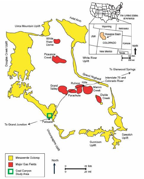
Figure 1: Map of gas-producing fields in Piceance Basin, Colorado (after EllisonEllison2004 ).

The Rulison Field, located in the South Piceance Basin, Garfield county, Colorado (Figure 1), produces gas from a 400 m thick pay section of channel sand lenses, stacked within the Cretaceous sandstones of the Mesaverde group. Porosities (from 1% to 10%) and permeabilities (from 1 $\mu$D to 60 $\mu$D) of these sand bodies characterize the formation as a tight gas reservoirRojas2005 . Because of such a low matrix permeability, it is believedJohnsonetal1987 ; Spencer1989 ; Lynnetal1999 that gas production is controlled by open natural fractures. Previous studiesLorenz2004 ; Jansen2005 suggest that fracture orientations vary over the field, and their intersections are thought to be important for the reservoir production. The average thickness of sand lenses is about 3 m, making them impossible to image with surface seismic data. As neither sand bodies nor fracture zones can be individually isolated on seismic images, it is necessary to characterize the fractures collectively as an effective medium. Reflector dips at the Rulison are small and can be neglected for the purposes of seismic data processing (Figure 2).

III.2 Data acquisition

A 3D, multicomponent seismic data set covering 2.2 km $\times$ 2.5 km was acquired by the Reservoir Characterization Project (Colorado School of Mines) in October, 2003 to characterize the Rulison Field with information from multiple sources (surface seismic, vertical seismic profiling, geomechanics, well logs, production data) and to monitor the changes in production and stresses with time-lapse measurements. For our study, we use the baseline wide-azimuth, 9C seismic survey. The sources are 3C (vertical and horizontal) vibrators placed at 33.5 m (110 ft) intervals along the lines oriented east-west; the crossline spacing is approximately 201 m (660 ft). The 3C receivers, 1500 Vectorseis^® digital accelerometers providing a total of 4500 live channels, are laid out in the north-south direction with 33.5 m (110 ft) inline and 101 m (330 ft) crossline intervals. This acquisition design yields an uncommonly high fold of about 500 in the middle of the survey and 200 to 300 on average.

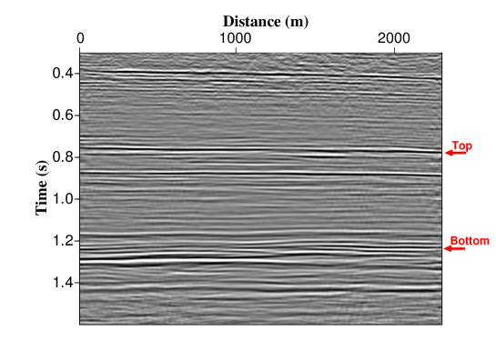
Figure 2: P-wave seismic section in east-west direction. Arrows mark the reflection events used for azimuthal velocity analysis.

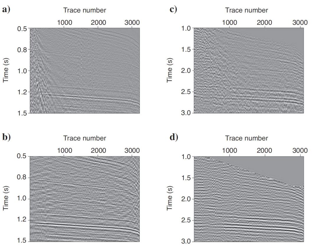
Figure 3: Representative input (a) and (c) and $f$-$k_{x}$-$k_{y}$-filtered (b) and (d) CMP gathers of the P- (left column) and S₁-waves (right column). Offsets increase with the increasing trace number. Both offsets and azimuths are irregularly sampled in the CMP domain.

III.3 Data processing

Our input data consist of three CMP-sorted volumes (P, S₁ and S₂), deconvolved for the source signature and corrected for the source-receiver statics. These pre-processing steps have been carried out by Veritas DGC prior to our project. In addition, ground-roll suppression turned out to be necessary. Strong surface waves, present in all three data volumes, are particularly harmful for the shear reflections (Figure 3). As the S-wave velocities are slower than the P-wave ones, shear events come later in time, and their greater offset interval is covered by the ground-roll (compare Figures 3a and 3c). To suppress it, we resort our irregularly sampled (in offsets and azimuths) data into shot and receiver lines, where the sampling is regular, and apply an $f$-$k_{x}$-$k_{y}$ filter that preserves the slopes up to 0.5 s/km. This approach to ground-roll suppression does not destroy azimuthal variations of traveltimes and results in a significant improvement of the reflected events (Figure 3).

Another pertinent issue concerns the two shear-wave volumes (S₁ and S₂) that we have at our disposal. The shear data have been rotated to the azimuth of the principal regional stress at N45E. Treating this azimuth as the orientation of one of the principal fracture sets implies a constant fracture azimuth throughout the field, in contradiction with the laterally variable orientations of the P-wave NMO ellipses observed from the bottom of the producing interval. To mitigate this discrepancy, we rotate the shear volumes to the principal directions of these P-wave NMO ellipses at each CMP location prior to performing the S-wave velocity analysis. The weak P-wave azimuthal anisotropy in the overburden, quantified by the eccentricities of the P-wave NMO ellipses consistently smaller than 3%, implies that fractures in the reservoir are the main source of the observed azimuthal anisotropy. If the latter is consistent with our theoretical model, the performed rotation brings the shear-waves to their principal directions; if not, such a rotation introduces some errors. These errors, however, are small for the majority of our data, as demonstrated in Figure 9 below.

After the ground-roll suppression and shear-wave rotation, we resort the data back to CMP geometry, create $9\times 9$ (135 m$\,\times\,$135 m) superbins and extract the NMO ellipses over the survey area. At each superbin location, estimation of the NMO ellipses is carried out around the zero-offset times that correspond to the reservoir top and bottom horizons (Figure 2), interpreted from the P, S₁, and S₂ image volumes. The NMO ellipses are computed at 5 ms time increments over a window centered at the horizon times. The averaging lengths of the semblance operators are 35 ms for the P-wave and 105 ms for the shear-wave data. Our use of the interpreted horizons for velocity analysis ensures the consistency of results with the geologically-based time structure.

We obtain the P-wave NMO ellipses over the entire survey area, the corresponding semblance values ranging from 0.55 to 0.65. As the shear data are noisier (compare Figure 3b with 3d), the S-wave NMO ellipses have been estimated for only about one third of the area. We discard the S-wave NMO ellipses whenever the semblances fall below 0.25. Indeed, the reflection events cannot be visually distinguished on the gathers with such low semblance values. On the other hand, in the higher-quality data areas, the azimuthal traveltime variations are clearly seen on the gathers corrected with an azimuthally-constant NMO velocity (Figure 4).

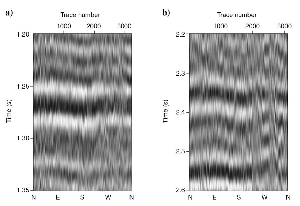
Figure 4: P- (a) and S₁-wave (b) gathers after the azimuthally-invariant NMO correction. The traces are sorted by the source-receiver azimuth. The apparent cosine-type dependence of the residual moveout is indicative of azimuthal anisotropy. The reflection events at approximately 1.27 s in (a) and 2.35 s in (b) correspond to the reservoir bottom.

After estimating the P, S₁, and S₂ NMO ellipses for the top and bottom horizons over the entire survey area, we proceed with the Dix-type differentiationGrechkaTsvankin1999 that yields the interval ellipses $\bm{W}_{\rm int}^{P}$, $\bm{W}_{\rm int}^{S1}$, and $\bm{W}_{\rm int}^{S2}$. Finally, minimizing the objective function in equation 6, we invert $\bm{W}_{\rm int}^{P}$, $\bm{W}_{\rm int}^{S1}$, and $\bm{W}_{\rm int}^{S2}$ and the interval zero-offset time ratios for the fracture parameters.

III.4 Fracture characterization

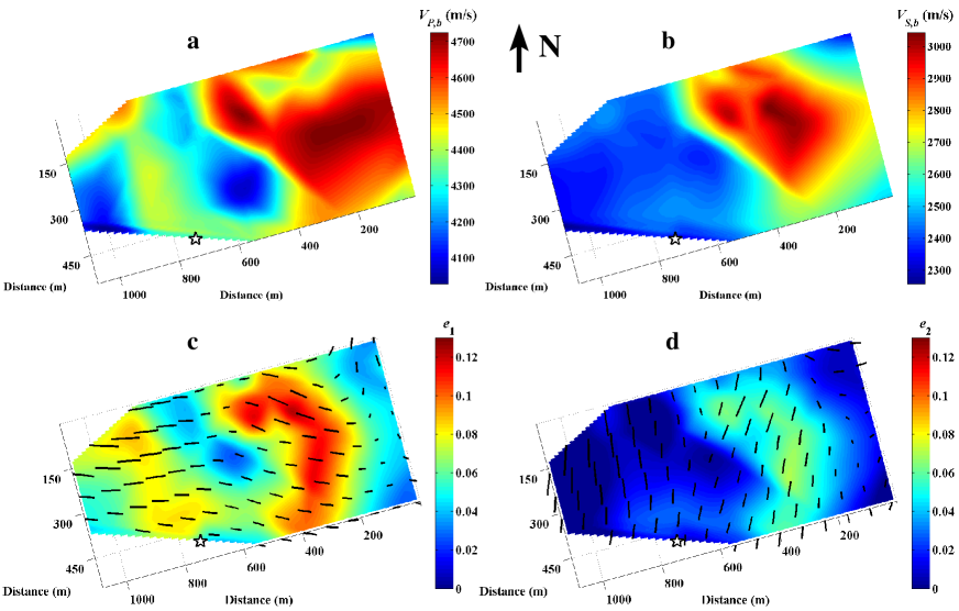
Figure 5: Output of the fracture characterization: the background velocities $V_{P,\,b}$ and $V_{S,\,b}$ of the P- (a) and S-waves (b), and the principal crack densities $e_{1}$ (c) and $e_{2}$ (d). The directions of the principal fracture sets are shown with the short black lines, their lengths proportional to the eccentricities of the interval P-wave NMO ellipses (shown in Figure 8b). These maps (as well as those in Figures 6–8) are the result of bi-cubic interpolation of the original data points spaced on a $9\times 9$ (135 m$\,\times\,$135 m) superbin grid. The stars indicate the location of well B. RWF 524-20, where an FMI log has been acquired (Figure 10).

Figure 5 displays the inverted background velocity fields $V_{P,\,b}$ and $V_{S,\,b}$ and the principal crack densities ${e}_{1}$ and ${e}_{2}$ (by definition, ${e}_{1}\geq{e}_{2}$). The crack densities in Figure 5c are considerably greater than those in Figure 5d, suggesting that the fracturing is dominated by the cracks trending in the WNW-ESE direction. Our results indicate that the western part of the area is mostly controlled by a single fracture set that has the density ${e}_{1}$, whereas the eastern part has a non-negligible contribution of other, differently oriented fractures that exhibit themselves as the set with the crack density ${e}_{2}$ (Figures 5c and 5d). We also observe that the areas of the highest crack densities do not necessarily coincide with the largest P-wave NMO ellipse eccentricities and revisit this issue later.

The background velocities (Figures 5a and 5b) show a sizable contrast between the eastern and western portions of the study area, with both P- and S-wave velocities being slower in the west. The fluid factors $\varsigma$ have been estimated also but we do not display them because all obtained values of $\varsigma$ are smaller than 0.01. These estimates are consistent with the fact that the Rulison Field produces dry gas.

III.5 Orthorhombic model of the reservoir

The estimated background velocities and crack densities (along with the fluid factors $\varsigma\approx 0$) are sufficient for building an orthorhombic depth model of the reservoir. Figures 6 and 7 display the vertical velocities $V_{P0}$ and $V_{S0}$ and Tsvankin’sTsvankin1997 anisotropy coefficients, their small-crack-density approximations found in Appendix A. We also present the anellipticity coefficients $\eta^{(1,\,2,\,3)}$ (the right column in Figure 7) to demonstrate that the predicted anisotropy is nearly elliptical.

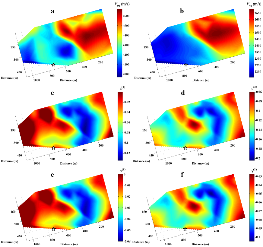
Figure 6: Vertical velocities (a) $V_{P0}$, (b) $V_{S0}$ and anisotropy coefficients (c) $\epsilon^{(1)}$, (d) $\epsilon^{(2)}$, (e) $\gamma^{(1)}$, and (f) $\gamma^{(2)}$ at Rulison reservoir.

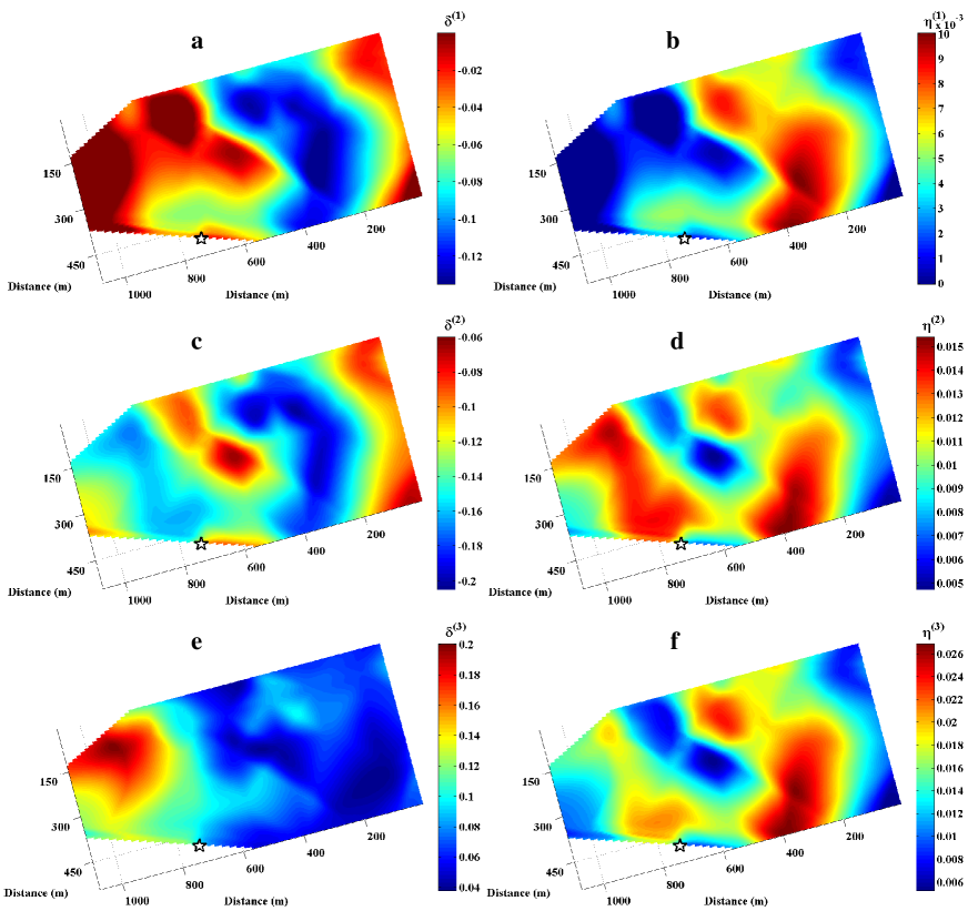
Figure 7: Anisotropy coefficients (a, c, e) $\delta^{(1,\,2,\,3)}$ and (b, d, e) $\eta^{(1,\,2,\,3)}$ at Rulison reservoir.

It is instructive to point out that the model in Figures 6 and 7 was obtained from reflection data only without the use of any borehole information to constrain the vertical depth scale. Although well-log or checkshot data are usually required for building orthorhombic subsurface models in depth domainGrechkaPechTsvankin2005 , we did not need such data in our study. The reason is that we explicitly target the crack-induced rather than general orthotropy. The former is significantly simpler because it is governed by fewer (five rather than nine) independent parameters, the reduction in the number of unknowns allowing us to rely solely on surface seismic data for building the unique orthorhombic model of the Rulison reservoir. As Figures 6 and 7 indicate, the reservoir is noticeably anisotropic: the magnitudes of anisotropy coefficients $\epsilon^{(2)}$ and $\delta^{(2)}$ reach 0.2 at the highest total crack density of $e=e_{1}+e_{2}=0.17$ (Figures 5c and 5d).

III.6 Conventional approaches to fracture characterization

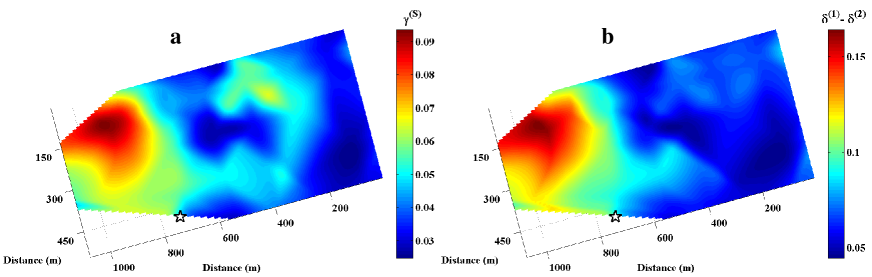
Figure 8: The shear-wave splitting coefficient $\gamma^{(\rm S)}$ (a) and the eccentricity of the P-wave NMO ellipses $\delta^{(1)}-\delta^{(2)}$ (b) at Rulison reservoir.

Having estimated the reservoir parameters from both P- and S-wave data, we can predict what would happen if we relied on either S- or P-waves alone for fracture characterization. In a typical pure shear-wave survey, one would measure the shear-wave splitting coefficient, $\gamma^{(\rm S)}\approx\gamma^{(1)}-\gamma^{(2)}$, and interpret it as the crack density of a single fracture set. The result of this interpretation in Figure 8a suggests that the western part of the study area is more fractured than the eastern one, quite opposite to the conclusion drawn from Figures 5c and 5d.

If only the P-wave data were usedGrechkaTsvankin1999 , one would estimate the eccentricity of the P-wave NMO ellipses, quantified by the difference of two $\delta$ coefficients, $\delta^{(1)}-\delta^{(2)}$. This difference, shown in Figure 8b, yields a similar result that the western part of the area is apparently more fractured than the eastern part.

The origin of these mutually contradictory conclusions can be understood from approximations 31 and 32. Clearly, both quantities $\gamma^{(\rm S)}$ and $\delta^{(1)}-\delta^{(2)}$ are proportional to the difference $\,e_{1}-e_{2}\,$ between the crack densities of two principal fracture sets. As a consequence, the shear-wave splitting coefficients and the eccentricities of the P-wave NMO ellipses are useful for fracture characterization only if one fracture set dominates, that is, when $e_{1}\gg e_{2}$. If multiple sets of cracks resulting in comparable $e_{1}$ and $e_{2}$ are present in the subsurface, both differences $\gamma^{(1)}-\gamma^{(2)}$ and $\delta^{(1)}-\delta^{(2)}$ become ambiguous. In particular, if the two principal crack densities coincide, $e_{1}=e_{2}\neq 0$, both differences vanish, $\gamma^{(1)}-\gamma^{(2)}=\delta^{(1)}-\delta^{(2)}=0$, and one would arrive to an obviously erroneous conclusion of the absence of fractures.

IV Verification of the results

An important part of any inversion procedure is assessment of errors in the estimated quantities. This section describes our efforts in this direction.

IV.1 Variances in data and estimated parameters

We estimated the data variances associated with uncertainties in traveltime picking. A plausible picking interval was defined in accordance with the autocorrelation function of traces in a CMP gather. Specifically, we take this interval to be equal to the time lag at which the autocorrelation drops by a factor of 10 from its zero-lag value. Such a definition yields the picking uncertainties equal to 8 ms for P- and 14 ms for S-waves. Next, a standard linear error-propagation technique is applied to translate these traveltime errors into uncertainties in the NMO ellipses. Finally, using the Fréchet-derivative matrix $\partial d_{j}/\partial m_{i}$, where $m_{i}$ and $d_{j}$ are the components of $\bm{m}$ and $\bm{d}$ (equations 4 and 5), we propagate the errors into the estimated quantities shown in Figure 5. This yields uncertainties of about 7% in the velocities $V_{P,\,b}$ and $V_{S,\,b}$ and 0.01 in the principal crack densities $e_{1}$ and $e_{2}$ at a 90% confidence interval. Given that eccentricities of the interval NMO ellipses are not large, we find the average errors in the ellipse azimuths to be equal to $12^{\circ}$, $17^{\circ}$, and $22^{\circ}$ for the P-, S₁-, and S₂-waves, respectively.

Estimation of the model variances is not the only resource for validating our results. As we have already mentioned, the fluid factors $\varsigma$ turned out to be nearly zero at all CMP locations, as expected because of the absence of production of liquids (oil or water) at the Rulison.

Another way of assessing the quality of our model assumptions is to analyze the misalignments in the orientations of the interval NMO ellipses for different wave modes. The histograms in Figure 9 exhibit pronounced peaks at zero, indicating that the ellipses are aligned at many CMP locations. Even though the presence of outliers (likely caused by noise in the data) makes average differences in the ellipse orientations of the P- and S₁-waves and the P- and S₂-waves be equal to 12^∘ and 17^∘, respectively, significant portion of the differences can be attributed to fracture interaction or, in seismic terminology, to multiple scattering of elastic energy by closely spaced cracks. For instance, Grechka and KachanovGrechkaKachanovORTfrac2006 found this mechanism to be responsible for the NMO ellipse misalignments up to 12^∘ at the total crack density $e=0.14$. Thus, we conclude that orientations of the NMO ellipses are consistent with our fracture model over most of the data.

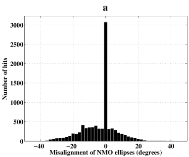
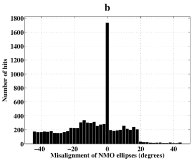
Figure 9: Histograms of azimuthal misalignments of the interval NMO ellipses of P- and S₁-waves (a) and P- and S₂-waves (b). The numbers along the vertical axes correspond to the interpolated values used to display the fracture-characterization results in Figures 5 – 7.

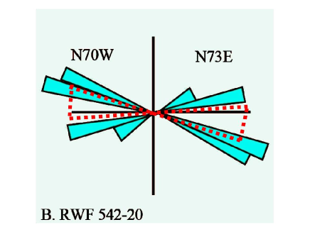
Figure 10: Fracture count (cyan) in well B. RWF 542-20 (marked by the star in Figures 5 – 8) and the 90% confidence interval (dotted red) corresponding to the azimuth of the fracture set with density ${e}_{1}$ estimated from seismic data.

IV.2 Borehole measurements

The survey area contains well B. RWF 542-20 (the star in Figures 5 – 8), where an FMI log was acquired, and fractures in the entire reservoir were counted. Figure 10 compares the borehole fracture count with our estimate of the crack orientation. As a dominant set of cracks has been identified at the well location (Figures 5c and 5d), we do not display the second set in Figure 10, for it has nearly zero crack density. The fractures observed in the FMI form two sets oriented approximately at N70W and N73E (cyan in Figure 10). Clearly, these sets are not orthogonal to each other; yet, their influence on the propagation of long (compared to the fracture sizes) seismic waves is equivalent to that of two orthogonal sets. The dotted red line in Figure 10 shows the azimuth of the dominant equivalent set estimated from seismic.

Figure 10 can be regarded as an illustration of the resolution achievable from seismic data: while long seismic waves cannot resolve each individual fracture set, they are sensitive to all fractures simultaneously. This cumulative influence of all cracks on elastic wave propagation is described by the crack-density tensorKachanov1980 ; GrechkaKachanovORTfrac2006 that can be represented in terms of contributions of mutually orthogonal (or principal) fracture sets that control the seismic signatures and can be estimated from them. Thus, returning to Figure 10, we state that our fracture-characterization results are consistent with the FMI log in well B. RWF 542-20.

V Discussion and conclusions

We have discussed seismic characterization of fractures at the Rulison Field, Colorado. To the best of our knowledge, Rulison is the first case study described in the geophysical literature, where parameters of multiple fracture sets — their orientations, crack densities, and the type of infill — have been estimated from multicomponent seismic reflection data. The key in our parameter-estimation methodology is the understanding, confirmed by extensive numerical modeling, that differently oriented, multiple vertical cracks appear as two orthogonal sets for long seismic waves. Following this understanding, we have targeted the parameters of those two orthogonal (or principal) sets in our inversion.

The obtained results point to a single fracture set oriented in the WNW-ESE direction in the western part of the study area and to two or more sets of cracks in its eastern part. These multiple sets yield the principal crack densities reaching $e_{1}=0.11$ and $e_{2}=0.06$ and implying an interconnected fracture network. This conclusion follows from a straightforward geometric consideration: it is extremely difficult to place two sets of orthogonal fractures that have random locations and the crack densities of $e_{1}=0.11$ and $e_{2}=0.06$ in a rock volume without letting those fractures intersect each other. Thus, our inversion has identified places in the reservoir, where swarms of intersecting cracks are likely to be present. Although multiple, differently oriented fracture sets might be viewed as contradictory to a common belief that only a single set of vertical open cracks directed along the regional stress field should exist in the subsurface, multiple fracture sets misaligned with the present stress directions have been observed in the Piceance BasinLaubachetal1998 ; Lorenz2004 and other areasLaubachetal2004 .

As a by-product of our fracture-characterization procedure, we have built an orthorhombic depth model of the Rulison reservoir. The reconstructed orthorhombic velocity model explicitly attributes the observed anisotropy to the presence of fractures. This rock-physics constraint reduces the number of independent quantities to be estimated and obviously improves the stability of inversion. In particular, it allows the vertical P- and S-wave velocities and all anisotropy coefficients to be uniquely determined solely from 3D, multiazimuth, multicomponent seismic reflection data. We believe that the Rulison is the first example of building an orthorhombic subsurface velocity model from seismic reflection data without using borehole information.

We paid special attention to verifying the obtained results. Here we list the supporting evidence.

(1) We propagated uncertainties in the picked zero-offset times and NMO ellipses into the quantities that characterize the fractures. This yielded errors of about 7% in the P- and S-wave velocities in the host rock and around 0.01 in the principal crack densities.

(2) The Rulison Field produces dry gas. While knowing this beforehand, we intentionally included the fluid factor into our unknowns. Its estimated values came out to be nearly zero in the entire study area, consistent with our prior information about of the type of fracture infill.

(3) The NMO ellipses of the P-, S₁-, and S₂-waves recorded from horizontal reflectors are supposed to be co-oriented according to the adopted non-interaction theory of crack-induced anisotropy. The ellipse misalignments observed in seismic data turned to be compatible with those predicted by numerical modeling that takes into account interaction of closely spaced fractures.

(4) The available FMI log confirmed the principal fracture azimuth estimated from seismic.

Despite the above assurances that the obtained results not only exhibit internal consistency but also fit some independent external data, comparison of our crack densities with the estimated ultimate recoveries of wells in the study area shows little correlation. The reason for that, we believe, is the physics of fluid flow through fractured rocks. For low-porosity (1% to 10%) sandstones at the Rulison, fracture networks appear to provide the main pathways for the gas flow. The effective, crack-related permeability of these networks is essentially controlled by the fracture widths, whereas the seismic signatures are governed by the crack densities or the fracture lengths. If a relationship between the crack widths and lengths is absent, the effective permeability and elasticity are uncorrelated. Perhaps, this is what we see at the Rulison.

Summarizing our seismic results, we reiterate that, to the best of our knowledge, our paper is the first to demonstrate the following:

• 3D, wide-azimuth, multicomponent seismic data can be used to characterize multiple vertical fracture sets in a purely isotropic host rock. The estimated crack densities might give an idea of where the fractures are likely to intersect and form interconnected networks.

• Orthorhombic subsurface models can be built from surface reflection data. We have shown that for a special case of crack-induced orthotropy, allowing us to resolve the time-depth ambiguity without relying on borehole data.

VI Acknowledgments

We thank the Reservoir Characterization Project (Colorado School of Mines) for providing seismic data and Shell E & P for permission to publish the paper. We are grateful to Jon Sheiman (Shell) for helping us with data processing, to Jorge Lopez (Shell), Ilya Tsvankin, Rodrigo Fuck (both CSM), and anonymous reviewers for their comments on the manuscript, and to Gerardo Franco and Xiaoxia Xu (both CSM) for useful discussions and suggestions. The work described in our paper has been carried out during summer internship of I. V. at Shell E & P in 2005.

Appendix A Small-crack-density approximations of seismic signatures

The goal of this Appendix is to develop an intuitive understanding of kinematic seismic signatures in formations containing multiple sets of vertical fractures. To arrive at tractable expressions, we assume that the principal crack densities are small, $\{e_{1},\,e_{2}\}\ll 1$, and linearize all pertinent quantities in $e_{1}$ and $e_{2}$. As stated in the main text, arbitrarily oriented fractures embedded in an otherwise isotropic host rock cause nearly orthorhombic effective symmetry, therefore, Tsvankin’sTsvankin1997 anisotropy coefficients introduced for orthorhombic media are of obvious importance for our study. We begin by deriving these anisotropy coefficients in terms of the governing parameters $\bm{m}$ (equation 4) and then turn our attention to the NMO ellipses of pure modes reflected from horizontal interfaces.

A.1 Anisotropy coefficients

As follows from equations 1 – 3, definition of the effective stiffness tensor, $\bm{c}_{e}=\bm{s}_{e}^{-1}$, and equations 16 – 19, 23 – 26 in TsvankinTsvankin1997 , the vertical velocities $V_{P0}$, $V_{S0}$ and relevant anisotropy coefficients, fully linearized in the crack densities, are:

$$V_{P0}=V_{P,\,b}\,\left[1+\frac{\,2\,\lambda_{b}^{2}\,(\varsigma-1)\,({e}_{1}+{e}_{2})}{3\,\mu_{b}\,(\lambda_{b}+\mu_{b})}\,\right],$$ (7)

$$V_{S0}=V_{S,\,b}\left(1-\frac{\,8\,}{3}\,\,e_{1}\,\frac{\lambda_{b}+2\,\mu_{b}}{3\,\lambda_{b}+4\,\mu_{b}}\right),$$ (8)

$$\epsilon^{(2)}=\frac{\,8\,}{3}\,\,{e}_{1}\,\left(\varsigma-1\right),$$ (9)

$$\epsilon^{(1)}=\frac{\,8\,}{3}\,\,{e}_{2}\,\left(\varsigma-1\right),$$ (10)

$$\delta^{(2)}=\frac{\,8\,}{3}\,\,{e}_{1}\left[\frac{\left(\varsigma-1\right)\,\lambda_{b}}{\lambda_{b}+\mu_{b}}-\frac{4\,\mu_{b}}{3\,\lambda_{b}+4\,\mu_{b}}\right],$$ (11)

$$\delta^{(1)}=\frac{\,8\,}{3}\,\,{e}_{2}\left[\frac{\left(\varsigma-1\right)\,\lambda_{b}}{\lambda_{b}+\mu_{b}}-\frac{4\,\mu_{b}}{3\,\lambda_{b}+4\,\mu_{b}}\right],$$ (12)

$$\gamma^{(2)}=-\frac{\,8\,}{3}\,\,{e}_{1}\,\frac{\lambda_{b}+2\,\mu_{b}}{3\,\lambda_{b}+4\,\mu_{b}}\,,$$ (13)

$$\gamma^{(1)}=-\frac{\,8\,}{3}\,\,{e}_{2}\,\frac{\lambda_{b}+2\,\mu_{b}}{3\,\lambda_{b}+4\,\mu_{b}}\,.$$ (14)

Here

$$V_{P,\,b}=\sqrt{\frac{\lambda_{b}+2\,\mu_{b}}{\rho}}$$ (15)

and

$$V_{S,\,b}=\sqrt{\frac{\mu_{b}}{\rho}}$$ (16)

are the velocities in the isotropic unfractured rock, $\rho$ is the mass density, and the quantities $\lambda_{b}$, $\mu_{b}$, $e_{1}$, $e_{2}$, and $\varsigma$ are described in the main text. Note that the anisotropy coefficients $\epsilon^{(2)}$, $\delta^{(2)}$, and $\gamma^{(2)}$, defined in the plane $[{x}_{1},\,{x}_{3}]$ that contains the normal to the first fracture set with the crack density $e_{1}$, are proportional to $e_{1}$ and independent of $e_{2}$. Likewise, the coefficients $\epsilon^{(1)}$, $\delta^{(1)}$, and $\gamma^{(1)}$ are controlled by $e_{2}$ only.

A.2 NMO ellipses and ratios of vertical velocities

Here we present the small-crack-density approximations for the data components (equation 5). The ratios of the vertical velocities are

$$\frac{V_{S1}}{V_{P0}} =\frac{V_{S0}}{V_{P0}}\,\sqrt{\frac{1+2\,\gamma^{(1)}}{1+2\,\gamma^{(2)}}}=\frac{V_{S,\,b}}{V_{P,\,b}}\,\Bigg{\{}1-\frac{2}{\,3\,\mu_{b}\,(\lambda_{b}+\mu_{b})}\,\Bigg{[}\lambda_{b}^{2}\,\left(\varsigma-1\right)\,e_{1}$$

$$\hskip 91.04881pt+\,\frac{(3\,\lambda_{b}+2\,\mu_{b})\,(\lambda_{b}^{2}\,\varsigma+4\,\mu_{b}^{2})-\lambda_{b}^{2}\,(3\,\lambda_{b}-2\,\mu_{b}\,\varsigma)}{3\,\lambda_{b}+4\,\mu_{b}}\,\,e_{2}\,\Bigg{]}\Bigg{\}}\,\qquad$$

and

$$\frac{V_{S2}}{V_{P0}} =\frac{V_{S0}}{V_{P0}}=\frac{V_{S,\,b}}{V_{P,\,b}}\,\Bigg{\{}1-\frac{2}{\,3\,\mu_{b}\,(\lambda_{b}+\mu_{b})}\,\Bigg{[}\lambda_{b}^{2}\,\left(\varsigma-1\right)\,e_{2}$$

$$\hskip 91.04881pt+\,\frac{(3\,\lambda_{b}+2\,\mu_{b})\,(\lambda_{b}^{2}\,\varsigma+4\,\mu_{b}^{2})-\lambda_{b}^{2}\,(3\,\lambda_{b}-2\,\mu_{b}\,\varsigma)}{3\,\lambda_{b}+4\,\mu_{b}}\,\,e_{1}\,\Bigg{]}\Bigg{\}}\,.\qquad$$

The pure-mode NMO ellipses from a horizontal reflector beneath a homogeneous orthorhombic layer are given byGrechkaTsvankin1998

$$\frac{1}{V_{Q,\,{\rm nmo}}^{2}(\phi)}=W_{Q,\,11}\,\cos^{2}\phi+W_{Q,\,22}\,\sin^{2}\phi=\frac{\cos^{2}\phi}{\left[V_{Q,\,{\rm nmo}}^{(1)}\right]^{2}}+\frac{\sin^{2}\phi}{\left[V_{Q,\,{\rm nmo}}^{(2)}\right]^{2}}\,.$$ (19)

In this equation, $Q=$ P, S₁, or S₂ is the wave type, $\phi$ is the azimuth measured from the normal to the first fracture set, $W_{Q,\,11}$ and $W_{Q,\,22}$ are the nonzero elements of the $2\times 2$ matrices $\bm{W}$ that describe general NMO ellipses, and $V_{Q,\,{\rm nmo}}^{(i)}$ are the symmetry-direction NMO velocities. These velocities are conveniently expressed in terms of the P- and S-wave vertical velocities and the anisotropy coefficients listed aboveGrechkaTheophanisTsvankin1999 :

$$V_{P,\,{\rm nmo}}^{(i)}=V_{P0}\,\sqrt{1\,+\,2\,\delta^{(i)}}\,,\quad(i=1,\,2)\,,$$ (20)

$$V_{S1,\,{\rm nmo}}^{(1)}=V_{S1}\,\sqrt{1+2\,\sigma^{(1)}}\,,$$ (21)

$$V_{S1,\,{\rm nmo}}^{(2)}=V_{S2,\,{\rm nmo}}^{(1)}=V_{S1}\,\sqrt{1+2\,\gamma^{(2)}}=V_{S2}\,\sqrt{1+2\,\gamma^{(1)}}\,,$$ (22)

$$V_{S2,\,{\rm nmo}}^{(2)}=V_{S2}\,\sqrt{1+2\,\sigma^{(2)}}\,,$$ (23)

where

$$\sigma^{(1)}=\left(\frac{V_{P0}}{V_{S1}}\right)^{2}(\epsilon^{(1)}-\delta^{(1)})\,,$$ (24)

$$\sigma^{(2)}=\left(\frac{V_{P0}}{V_{S2}}\right)^{2}(\epsilon^{(2)}-\delta^{(2)})\,.$$ (25)

Substitution of equations 7 – 16 in equations 20 – 25 and subsequent linearization yields

$$V_{P,\,{\rm nmo}}^{(1)} =V_{P,\,b}\,\Bigg{\{}1+\frac{2}{\,3\,\mu_{b}\,(\lambda_{b}+\mu_{b})}\,\Bigg{[}\lambda_{b}^{2}\,\left(\varsigma-1\right)\,e_{1}$$

$$+\,\frac{1}{3\,\lambda_{b}+4\,\mu_{b}}\,\left(3\,\lambda_{b}^{3}\,\left(\varsigma-1\right)+16\,\mu_{b}\,\left(\lambda_{b}^{2}\,\left(\varsigma-1\right)+\lambda_{b}\,\mu_{b}\,\left(\varsigma-2\right)-\mu_{b}^{2}\right)\right)e_{2}\,\Bigg{]}\Bigg{\}}\,,\qquad$$

$$V_{P,\,{\rm nmo}}^{(2)} =V_{P,\,b}\,\Bigg{\{}1+\frac{2}{\,3\,\mu_{b}\,(\lambda_{b}+\mu_{b})}\,\Bigg{[}\lambda_{b}^{2}\,\left(\varsigma-1\right)\,e_{2}$$

$$+\,\frac{1}{3\,\lambda_{b}+4\,\mu_{b}}\,\left(3\,\lambda_{b}^{3}\,\left(\varsigma-1\right)+16\,\mu_{b}\,\left(\lambda_{b}^{2}\,\left(\varsigma-1\right)+\lambda_{b}\,\mu_{b}\,\left(\varsigma-2\right)-\mu_{b}^{2}\right)\right)e_{1}\,\Bigg{]}\Bigg{\}}\,,\qquad$$

$$V_{S1,\,{\rm nmo}}^{(1)}=V_{S,\,b}\left\{1+\frac{\,8\,(\lambda_{b}+2\,\mu_{b})}{3\,(\lambda_{b}+\mu_{b})}\,\,{e}_{2}\,\left[\varsigma-\frac{\mu_{b}}{3\,\lambda_{b}+4\,\mu_{b}}\,\right]\right\},$$ (28)

$$V_{S1,\,{\rm nmo}}^{(2)}=V_{S2,\,{\rm nmo}}^{(1)}=V_{S,\,b}\left[\,1-\frac{8\,(\lambda_{b}+2\,\mu_{b})}{3\,(3\,\lambda_{b}+4\,\mu_{b})}\,\left(e_{1}+{e}_{2}\right)\,\right],$$ (29)

$$V_{S2,\,{\rm nmo}}^{(2)}=V_{S,\,b}\left\{1+\frac{\,8\,(\lambda_{b}+2\,\mu_{b})}{3\,(\lambda_{b}+\mu_{b})}\,\,{e}_{1}\,\left[\varsigma-\frac{\mu_{b}}{3\,\lambda_{b}+4\,\mu_{b}}\,\right]\right\}.$$ (30)

It is a simple matter now to construct the Fréchet-derivative matrix, $\bm{F}$, of the quantities given by equations A.2, A.2, and A.2 – 30 with respect to the elements of parameter vector $\bm{m}$ (equation 4) and verify that all singular values of $\bm{F}$ are nonzero.

A.3 Shear-wave splitting coefficient and the eccentricity of P-wave NMO ellipse

Finally, we use the already derived approximations to demonstrate that such well-known fracture indicators as the shear-wave splitting coefficient and the eccentricity of P-wave NMO ellipse are controlled by the difference of two principal crack densities, $e_{1}-e_{2}$, and, therefore, insufficient for characterization of multiple fracture sets.

The eccentricity (or normalized elongation) of the P-wave NMO ellipse is just the difference between two $\delta$ coefficients. As follows from equations 11 and 12, the eccentricity is

$$\delta^{(1)}-\delta^{(2)}=\frac{\,8\,}{3}\,\,(e_{1}-{e}_{2})\left[\frac{\left(1-\varsigma\right)\,\lambda_{b}}{\lambda_{b}+\mu_{b}}+\frac{4\,\mu_{b}}{3\,\lambda_{b}+4\,\mu_{b}}\right]\,.$$ (31)

Similarly, definition of the shear-wave splitting coefficient, $\gamma^{(\rm S)}\approx\gamma^{(1)}-\gamma^{(2)}$, and equations 13, 14 yield

$$\gamma^{(\rm S)}=\frac{\,8\,}{3}\,\,(e_{1}-{e}_{2})\,\,\frac{\lambda_{b}+2\,\mu_{b}}{\,3\,\lambda_{b}+4\,\mu_{b}}\,.$$ (32)

These signatures unambiguously constrain the crack density only for a single fracture set, that is, when $e_{2}=0$.

References

- (1) P. Berthet, J.-P. Dunand, P. Julien, and J. Arnaud, Summer Research Workshop, SEG/EAGE, Vancouver, British Columbia, Canada (2004).
- (2) A. A. del Monte, E. Angerer, C. Reiser, and C. Glass, Summer Research Workshop, SEG/EAGE, Vancouver, British Columbia, Canada (2004).
- (3) D. Gray and D. Todorovic-Marinic, Summer Research Workshop, SEG/EAGE, Vancouver, British Columbia, Canada (2004).
- (4) B. J. Minsley, M. E. Willis, M. Krasovec, D. R. Burns, and M. N. Toksöz, Summer Research Workshop, SEG/EAGE, Vancouver, British Columbia, Canada (2004).
- (5) D. Todorovic-Marinic, G. Larson, D. Gray, G. Soule, Y. Zheng, and J. Pelletier, Summer Research Workshop, SEG/EAGE, Vancouver, British Columbia, Canada (2004).
- (6) J. E. Gaiser and R. R. Van Dok, Summer Research Workshop, SEG/EAGE, Vancouver, British Columbia, Canada (2004).
- (7) S. E. Laubach, J. E. Olson, and J. F. W. Gale, Earth and Planetary Science Letters 222, no. 1, 191 (2004).
- (8) V. Grechka and I. Tsvankin, Geophysics 65, 1399 (2004).
- (9) M. Schoenberg, Journal of the Acoustical Society of America 68, no. 5, 1516 (1980).
- (10) A. Bakulin, V. Grechka, and I. Tsvankin, Geophysics 65, no. 6, 1803 (2000).
- (11) M. Kachanov, Journal of the Engineering Mechanics Division, ASCE 106, 1039 (1980).
- (12) M. Schoenberg and C. Sayers, Geophysics 60, 204 (1995).
- (13) M. Kachanov, Hutchinson, J. W., and T. Wu, eds., Advances in Applied Mechanics (Academic Press, 1993), pp. 259–445.
- (14) V. Grechka and M. Kachanov, Geophysics 71, no. 3, D93 (2006).
- (15) V. Grechka and M. Kachanov, Geophysics 71, no. 3, D85 (2006).
- (16) V. Grechka, I. Vasconcelos, and M. Kachanov, Geophysics 71, no. 5, D153 (2006).
- (17) V. Grechka and I. Tsvankin, Geophysics 63, no. 3, 1079 (1998).
- (18) V. Grechka, S. Theophanis, and I. Tsvankin, Geophysics 64, no. 1, 146 (1999).
- (19) I. Tsvankin, Geophysics 62, no. 4, 1292 (1997).
- (20) V. Grechka and I. Tsvankin, Geophysics 64, no. 4, 1202 (1999).
- (21) I. Vasconcelos and I. Tsvankin, Geophysical Prospecting 54, 535 (2006).
- (22) E. Jenner, Ph.D. thesis, Colorado School of Mines (2001).
- (23) A. I. Ellison, MSc. thesis, University of Colorado (2004).
- (24) E. Rojas, MSc. thesis, Colorado School of Mines (2005).
- (25) R. C. Johnson, R. A. Crovelli, C. W. Spencer, and R. F. Mast, U.S. Geological Survey Open-File Report 87-357 (1987).
- (26) C. W. Spencer, American Association of Petroleum Geologists Bulletin 73, no. 5, 613 (1989).
- (27) H. B. Lynn, D. Campagna, K. M. Simon, and W. E. Beckham, 64, 1293 (1999).
- (28) J. C. Lorenz, Piceance Basin guidebook (Rocky Mountain Association of Geologists, 2004), pp. 75–94.
- (29) K. Jansen, MSc. thesis, Colorado School of Mines (2005).
- (30) V. Grechka, A. Pech, and I. Tsvankin, Geophysics 70, no. 1, D1 (2005).
- (31) S. E. Laubach, R. Marrett, J. E. Olson, and A. R. Scott, International Journal of Coal Geology 35, 175 (1998).