A Comparison of Photometric Redshift Techniques for Large Radio Surveys
Abstract
Future radio surveys will generate catalogues of tens of millions of radio sources, for which redshift estimates will be essential to achieve many of the science goals. However, spectroscopic data will be available for only a small fraction of these sources, and in most cases even the optical and infrared photometry will be of limited quality. Furthermore, radio sources tend to be at higher redshift than most optical sources (most radio surveys have a median redshift greater than ) and so a significant fraction of radio sources hosts differ from those for which most photometric redshift templates are designed. We therefore need to develop new techniques for estimating the redshifts of radio sources. As a starting point in this process, we evaluate a number of machine-learning techniques for estimating redshift, together with a conventional template-fitting technique. We pay special attention to how the performance is affected by the incompleteness of the training sample and by sparseness of the parameter space or by limited availability of ancillary multi-wavelength data. As expected, we find that the quality of the photometric-redshift degrades as the quality of the photometry decreases, but that even with the limited quality of photometry available for all sky-surveys, useful redshift information is available for the majority of sources, particularly at low redshift. We find that a template-fitting technique performs best in the presence of high-quality and almost complete multi-band photometry, especially if radio sources that are also X-ray emitting are treated separately, using specific templates and priors. When we reduced the quality of photometry to match that available for the EMU all-sky radio survey, the quality of the template-fitting degraded and became comparable to some of the machine learning methods. Machine learning techniques currently perform better at low redshift than at high redshift, because of incompleteness of the currently available training data at high redshifts.
1 Introduction
Next-generation radio surveys will generate catalogues of tens of millions of galaxies (Norris, 2017b). Much of the science generated by these surveys depends on the availability of identifications and redshifts for each radio source. However, in spite of recent advances, even multi-object spectroscopy can only provide redshifts for a small fraction of these galaxies. Instead, only photometric redshifts (hereafter photoz’s) can provide the necessary redshift information for the large samples of radio sources.
In this context we focus on an extensive radio survey, the Evolutionary Map of the Universe (EMU), which has been designed to use the new ASKAP radio telescope to make a deep (/beam target rms) radio survey covering the entire Southern Sky and extending as far North as (Norris et al., 2011). EMU aims to detect about million sources, about half of which are expected to be star-forming galaxies and the rest Active Galactic Nuclei (AGN). EMU’s key science goals include tracing the evolution of galaxies from the early Universe to the present day, and using the distribution of radio sources to explore the large-scale structure and cosmological parameters of the Universe. These goals require redshift estimates for a significant fraction of the sources. In particular, AGN represent an important challenge to photometric redshift techniques (see Salvato et al., 2018, for a review).
Since the early pioneering work (Baum, 1962; Butchins, 1981; Loh & Spillar, 1986), many different methods to evaluate photoz’s have been implemented and extensively tested on a wide range of data. A comprehensive review of these techniques has recently been published by Salvato et al. (2018).
All these methods use some a-priori knowledge gained either from spectroscopy or from physical assumptions, to deduce the function that maps the parameter space of photometric observables onto the spectroscopic redshift distribution. Methods can be roughly divided into two categories: (i) SED (Spectral Energy Distribution) template fitting, and (ii) machine learning (ML) techniques.
Template fitting techniques (e.g. Arnouts et al., 1999; Benítez, 2000; Bolzonella et al., 2011; Brammer et al., 2010; Duncan et al., 2018a) rely on a library of template galaxy spectra which are then shifted to different redshifts and fitted to the observed photometric data points. The various implementations differ in the way the template library is assembled (from real galaxy spectra or from synthetic spectra), in the possible inclusion of emission lines (crucial to model AGN and starburst spectra), and on the ability to use priors and in the fitting procedure adopted. The techniques used to extract the photometric measurements, the number of bands, and the simultaneity of the measurements can all profoundly affect the photoz accuracy. For example, single band extractions give worse redshifts than combined extractions. Most template fitting techniques do not use wavelengths longer than the infrared, since the templates are not well defined at longer wavelength. Notable exceptions are Rowan-Robinson et al. (2008) who used early IRAC data up to 8m from the SWIRE survey, Aretxaga et al. (2007) who used radio and far-infrared data, and Pearson et al. (2013) who used Herschel and sub-mm data. Here we use the Le Phare (Arnouts et al., 1999; Ilbert et al., 2006) code (see Section 4.1) with optical and near-infrared data.
Machine learning (ML) based techniques first introduced by Tagliaferri et al. (2003); Firth et al. (2002), use the a-priori knowledge from a “training set” of objects (also known as a Knowledge Base or KB) for which accurate spectroscopic redshifts are available. Implementations include random forest, neural networks, nearest neighbours, support vector machines, Gaussian process regression, and self-organised maps. Recent developments include the ability to generate probability density functions (PDFs) for the redshifts, rather than a single most likely point estimation (Amaro et al., 2017, 2018; Duncan et al., 2018b), and the ability to take account of spectral variability (Pasquet-Itam & Pasquet, 2017). Masters et al. (2015) also discuss the effect of the biases introduced by the a priori information.
Several studies have compared the relative merits of ML and template approaches (Hildebrandt et al., 2008; Dahlen et al., 2013; Abdalla et al., 2011). For example, ML methods cannot effectively estimate photometric redshifts for objects fainter than the spectroscopic limit, or for rare objects that are not represented in the training sample. Throughout this paper, and for all foreseeable ML applications, the training data and the target data must be limited to the same limiting magnitude. Template fitting methods can estimate redshifts of rare or peculiar objects as long as a representative template is included in the library. Key advantages of the template fitting methods are: (i) they can be extrapolated beyond the spectroscopic limit and, (ii) they can provide an estimate of the galaxy spectroscopic type and thus morphology, providing by default (iii) also a quality of the fit. Template fitting procedures also provide a redshift probability distribution function, which has only recently become available from ML codes.
However, if the KB samples the observed parameter space well, and the properties of sources in the KB closely match those in the target data, ML methods can be more accurate than template fitting. Furthermore, they do not require an a priori hypothesis about the underlying physics, and they can use non-photometric information such as morphology, radio polarization, photometric gradients (Gieseke et al., 2011; Norris et al., 2013) or even the spectroscopic type provided by template fitting procedures (Cavuoti et al., 2017).
The complementary nature of the two techniques have also inspired approaches that use a hybrid of SED fitting and machine learning in a single collaborative framework, which improve the accuracy of photoz estimates (e.g. Cavuoti et al., 2017b; Duncan et al., 2018b).
The quality of photoz’s might be expected to improve with the depth of the data and thus a smaller photometric error, the number of the bands available, and a decreasing spacing between the filters (e.g. Budavári & Szalay, 2008; Benítez et al., 2009). While this is usually true for template fitting methods, this is not necessarily true for ML methods where additional parameters, or features, may increase the noise and decrease performance. For example, increasing the number of bands may increase the incompleteness of the data, and reduce the density of training points in the parameter space, thereby increasing the noise in the photoz’s. Instead, the choice of the features to be used should be optimized by a feature selection phase (Brescia et al., 2013; D’Isanto et al., 2018). Polsterer et al. (2014) and Cavuoti et al. (2014) have shown that, assuming that the automatic feature selection can identify crucial parameters, feature selection should be data-driven rather than driven by astronomical reasoning.
Most studies comparing the performance of photoz methods have been based on optically-selected samples, omitting outlier sources such as AGN and Starburst galaxies, which dominate radio-selected samples. Furthermore, the median redshift of sources found in EMU is expected to be z 1.2, which is very different from the median redshift z 0.2 of most wide optical surveys (Norris et al., 2011). Most of the high-redshift radio sources are high-z radio-loud AGN, which are relatively rare in optical surveys because they are faint at optical wavelengths. For example, about half the sources in modern radio surveys host an AGN (Norris et al., 2013), most of which are detected only in very deep X-ray surveys (La Franca et al., 2012; Smolčić et al., 2017).
In template fitting techniques, the choice of the library of templates plays a crucial role. While a standard library can be used for computing photoz for normal galaxies at any redshift and depth, alternative templates must be considered when working on radio or X-ray selected sources. In particular, for X-ray sources, the library of templates change with the depth of the X-ray survey (e.g. Salvato et al., 2011; Hsu et al., 2014).
Furthermore, current templates generally do not use wavelengths beyond 5 m whereas ML methods can use radio, IR, and X-ray data to improve the photoz accuracy.
An additional challenge that is faced when computing photoz for large radio surveys such as EMU, is that the photometry will heterogeneous, using different photometric catalogs of different depths. This is in contrast to deep optical pencil-beam surveys, where images are registered to the same astrometric frame and the photometry is then measured with the same aperture, taking into account the different point spread functions. For example, Table 4 compares the photometric data that is avaialable for COSMOS and that is predicted will be available for EMU.
As a result, comparisons of photometric redshift techniques performed on optically-selected samples do not necessarily reflect their performance on radio-selected samples. This is addressed by Duncan et al. (2018a, b), whose work is complementary to this paper. Duncan et al. use a different regression technique from any used here (Gaussian process regression, or Kliging) but, more importantly, divide their data into several classes (star-forming, IR AGN, etc) and separately train their algorithms on these classes, and combine the results from the different sets, together with the results from template fitting, using a Bayesian estimator. This combination of results is very successful, but here our focus is different. While we want to quantify the quality of the photoz that will be available for EMU and compare it with what is available for pencil beam surveys, we also want to understand whether flagging the sources that are known to be X-ray or variable AGN can improve the results. Finally, we want to see whether using radio and X-ray fluxes can improve the performances of ML algorithms. We do this in the COSMOS field, comparing the performance of a number of photoz techniques, on a sample of sources detected in radio, at the same depth that will be available for COSMOS.
Previous analysis of this field based on filters ( broad bands, narrow bands and intermediate bands) with a typical depth of mag (AB) allowed template fitting methods to predict photoz’s with an accuracy better than for normal galaxies (Ilbert et al., 2009) and for a sample of X-ray selected galaxies (Salvato et al., 2009, 2011).
In this paper, §2 presents the data and overall experimental approach; §3 describes the individual methods, §4 describes the methods and tests, and §5 presents the 16 cases that we tested. In §6 and §7 we compare and discuss the results from the various methods.
2 The data
The data from the COSMOS project are publicly available111http://irsa.ipac.caltech.edu/data/COSMOS/ and provide an ideal benchmark for this project (Scoville et al., 2007). COSMOS covers a sq. deg. field: an area large enough to reduce cosmic variance and to sample the bright and rare objects. It has a large spectroscopic follow-up pursued using optical and near-infrared spectrographs mounted on the largest telescopes available, curated into a master spectroscopic catalog by Salvato, thus increasing the sampling completeness. It has deep, multi-epoch multi-wavelength observations from X-ray (XMM, Chandra) to radio (VLA), including UV (Galex, Zamojski et al. (2007), optical (broad band photometry from SDSS, CFHT, intermediate and narrow band photometry from SUBARU (Taniguchi et al., 2007)), NIR and MIR (McCracken et al., 2010; Sanders et al., 2007, Ultravista and Spitzer-IRAC bands)). The data are highly homogeneous, since images have been registered to a common grid and convolved to a common PSF and fluxes computed in a common aperture. When this work started, the only multiwavelength COSMOS catalog available (Ilbert et al., 2009) reported magnitudes instead of fluxes like the latest version (Laigle et al., 2016). This added a complication to the computation of the photoz, for both SED fitting and ML algorithms. All data have been corrected for extinction, and magnitudes (AB) are computed in a arcsec aperture.
The COSMOS survey is complemented by VLA (Schinnerer et al., 2007, 2010) XMM-Newton (Hasinger et al., 2007; Brusa et al., 2010) and Chandra (Civano et al., 2012) observations. VLA-COSMOS provides radio coverage of the field with roughly the same depth and resolution expected for EMU. The COSMOS field is currently being surveyed to an even greater depth using the VLA(Smolčić et al., 2017) but those data are not used in this paper. Herrera Ruiz et al. (2017) have observed all these sources with VLBI, and confirm that a significant fraction of them are high-redshift radio-loud AGN. Sargent et al. (2010) argue that 99.9% of the VLA-COSMOS data have a secure optical counterpart, although, since some of the radio sources are likely to be very high redshift radio-loud AGN, which are extremely faint at optical/IR wavelengths, a small fraction of these are likely to be mis-identifications.
The VLA-COSMOS GHz sample consists of sources with optical counterparts (Sargent et al., 2010). In this paper, we use as our primary set a subsample of sources that have reliable spectroscopic redshifts. We call this our “spectroscopic KB”. Of the sources in the KB, have X-ray fluxes measured by XMM (Brusa et al., 2010) and an additional (i.e. excluding those also detected by XMM) have X-ray fluxes measured by Chandra (Civano et al., 2012; Marchesi et al., 2016).
From this vast array of data, a total of different photometric measurements, or “features”, were used in the experiments here and are listed in Table 5. Except where stated otherwise, all data were used in all experiments.
3 Experimental approach
We ran the experiment as a “blind data challenge”, in which different groups (all of whom are co-authors of this paper) were invited to test their algorithms on the KB, with the challenge being run by a control group. Machine learning techniques require the KB to be split into two subsets called the ’training’ and ’test’ set respectively. These two subsets need to be disjoint and to map the parameter space representatively. For the experiments described here, the control group provided the testers with the training set, which includes redshifts, and the blind test set, which does not include redshifts. The testers then used the training set to train their algorithms. The trained algorithms were then applied to the test set to yield a set of estimated redshifts. These were then passed back to the control group who compared them with the true spectroscopic redshifts, to evaluate the algorithms in terms of standard statistical indicators.
As well as evaluating the test on the best data available, we are interested in the sensitivity of the tests to the number of bands available, the sensitivity of the photometry, whether radio flux density is used, and whether X-ray detected AGN are included in the training sets. These tests were therefore varied in four ways:
-
•
Variation 1: Bias: In general, spectroscopy tends to be available on sources that are brighter than the population of sources for which we wish to obtain photometric redshifts. Here we test the ability of the techniques to train on a brighter sample of sources and extrapolate that training to a larger sample containing fainter sources. We therefore performed two variations: In the “Bright” variation, the training set was chosen to be the optically brightest % of sources, selected in the band. In the “Random” variation, the training set was randomly chosen from the parent sample of objects. In both cases, because of an implementation detail, the fraction was not exactly half. In the “Bright” variation, sources were in the training set, and were in the test set. In the “Random” variation, sources were in the training set, and were in the test set.
-
•
Variation 2: Depth As discussed in Sec. 1, all-sky photometry surveys will be much shallower than the deep data available in pencil-beam fields such as COSMOS. For example, over most of the area of EMU, the only optical/infrared surveys (listed in Table 4 along with their limiting magnitudes), available in the next year will be the SkyMapper(Wolf et al., 2018), ALLWISE (Wright et al., 2010), and VHS (McMahon et al., 2013), while smaller but still significant areas will be covered by DES (Dark Energy Survey Collaboration et al., 2016) and other surveys. This will introduce incompleteness in these large surveys, and a significant fraction of objects will only have upper limits on their photometry in some bands. At X-ray wavelengths, eROSITA (Merloni et al., 2012) will provide an all-sky catalog that is expected to be about 30 times deeper than ROSAT (Boller et al., 2016), which is still much shallower than XMM-COSMOS, for example. We simulated this effect by performing two variations. In the “Deep” variation, the training set used the deepest data available in the KB. For example, these data include the Spitzer-IRAC measurements (Sanders et al., 2007), which are available only in small regions of the sky. In the “Shallow” variation, the training set used shallower data to simulate the data available to the EMU survey. Specifically, (i) Spitzer-IRAC data was limited to bands and and to the depth of the ALLWISE data (Wright et al., 2010), and (ii) optical photometry data for sources fainter than was removed, i.e. keeping the sources that are about 1 magnitude fainter than what is expected for the final depth of SkyMapper. For the same reason, we also included only broad band photometry in the “Shallow” data, removing narrow and intermediate band photometry. None of these reductions in the quality of the data affected the size of the training (, ) and test (, ) sets. However, these changes typically removed optical photometry for about one third of sources, and infrared photometry for about two thirds of sources.
-
•
Variation 3: Radio: template fitting techniques typically do not use wavelengths longer than the mir-infrared, since the templates are not well defined at long wavelengths. However, ML methods can in principle use radio data too. To our knowledge, no systematic study of whether the radio fluxes may be used to help constrain photoz’s has been performed using ML methods. To see if the inclusion of radio data made a difference, testers were asked to incorporate radio data in their tests in the “radio=Y” variation, and to ignore them in the “radio=N” variation. This did not affect the size of the training and test sets.
-
•
Variation 4: X-ray AGN: In previous template fitting in the COSMOS (e.g. Salvato et al., 2009), X-ray detected sources were treated differently, by using different libraries and priors. Here we test how ML techniques are affected by the presence of these sources and whether knowing in advance that they are AGN can help to improve the results. To see if the presence of AGN affected the results, X-ray AGN detected by XMM were excluded from the training sets in the “X-ray=N” variation, and included in the “X-ray=Y” variation. However, it should be noted that since most radio-loud AGN are not detected in X-rays, this test does not remove all AGN. Furthermore, Chandra data in this field were not available at the time of these tests and so were not used in this process. As a result of this variation, the size of the training set used in the “X-ray=N” tests was reduced to and objects respectively in the “bright” and “random” samples, and the size of the test set was correspondingly increased to and .
These four variations are not independent and so each of them must be combined along with the other variations. The combination of these variations resulted in a set of experiments, listed in Table 1, which shows the size of the training and test sets and the number of features. In all cases (except for Le Phare), the tests were trained on the training set provided, and then applied to the entire test set, which includes members of the training set. The control group then removed the sources in the training set from the test set before evaluating the results. Le Phare was tested only in the variation 1,2,4, with X-ray detected AGN either treated as galaxies (X-ray=N), or separately (X-ray=Y).
In Figure 1 we show the resulting magnitude and redshift distribution for the bright and random training and test sets. We also report the magnitude distribution of the entire sample.
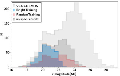
a)
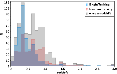 b)
b)
For consistency in this paper, we adopt the following terminology. An “experiment” is one of the sixteen listed in Table 1. A “test” occurs when one of these experiments is undertaken by one of the six “methods” listed in Sec. 4.
| Id. | CODE | KB bias | depth | Radio | X-ray | # training | # test | # training |
|---|---|---|---|---|---|---|---|---|
| sources | sources | features | ||||||
| A1 | BDNY | Bright | Deep | N | Y | 391 | 366 | 44 |
| B1 | BDYY | Bright | Deep | Y | Y | 391 | 366 | 45 |
| C1 | BDNN | Bright | Deep | N | N | 302 | 455 | 44 |
| D1 | BDYN | Bright | Deep | Y | N | 302 | 455 | 45 |
| E1 | BSNY | Bright | Shallow | N | Y | 391 | 366 | 44 |
| F1 | BSYY | Bright | Shallow | Y | Y | 391 | 366 | 45 |
| G1 | BSNN | Bright | Shallow | N | N | 302 | 455 | 44 |
| H1 | BSYN | Bright | Shallow | Y | N | 302 | 455 | 45 |
| A2 | RDNY | Random | Deep | N | Y | 343 | 414 | 44 |
| B2 | RDYY | Random | Deep | Y | Y | 343 | 414 | 45 |
| C2 | RDNN | Random | Deep | N | N | 278 | 479 | 44 |
| D2 | RDYN | Random | Deep | Y | N | 278 | 479 | 45 |
| E2 | RSNY | Random | Shallow | N | Y | 343 | 414 | 44 |
| F2 | RSYY | Random | Shallow | Y | Y | 343 | 414 | 45 |
| G2 | RSNN | Random | Shallow | N | N | 278 | 479 | 44 |
| H2 | RSYN | Random | Shallow | Y | N | 278 | 479 | 45 |
4 The methods
We used the Le Phare template fitting method as a baseline. and compared four different machine learning based methods with it: the k-nearest neighbours (kNN), two different implementations of Random Forest (RF), and the Multi Layer Perceptron with Quasi Newton Algorithm (MLPQNA). Here we discuss the implementation of each of them.
For each ML test, the method used the training sets whose size is shown in Table 1, and the test sets consisted of all members of the KB that were not included in the training set. The size of the test set for each experiment is shown at the top of Table 3. The number of redshifts estimated is generally lower than this number, for two reasons. First, each algorithm has different ways of handling missing values. The Dameware platform, used by RF-NA and MLPQNA, removes features or objects for which data are missing, resulting in the reduced size of the data sets shown in Table 2. kNN also omitted objects with missing values, but where possible used subspaces of features that were detected to measure an alternative kNN distance. The R platform, used by RF-JHU, uses the rfimpute function which replaces missing values by a weighted average of those with similar redshift using another random forest. Furthermore, before analysing the results, we removed from the test set any invalid results in which the method had failed, as indicated by a (Not-a-Number) in the estimated redshift. The actual number of valid results in the test set for each test is indicated by N in each entry of Table 3.
4.1 Le Phare
The Le Phare code is public222http://www.cfht.hawaii.edu/~arnouts/LePhare/LePhare.html (Arnouts et al., 1999; Ilbert et al., 2006) and has been extensively tested (Hildebrandt et al., 2008; Dahlen et al., 2013; Cavuoti et al., 2017; Santini et al., 2015, e.g.,) for photoz and stellar mass computations. It is also the code used by the COSMOS collaboration. In this way we can easily compare the results between radio and optically selected galaxies. Le Phare can account for the intergalactic medium, and for the contribution of the emission lines to the templates. The code also allows the use of various types of priors. Here we used the absolute magnitude, which enables better constraints on the photometric redshifts of AGN (Salvato et al., 2009, 2011, e.g.,). The photometric redshift can be computed either by minimising the (zBEST), or by marginalising over the best solution for each of the templates in use (). In both cases, in addition to the (zBEST) and (), and upper and lower errors are computed, together with the probability distribution function P(z). Le Phare shares the properties of most common SED template fitting methods (e.g., Hildebrandt et al., 2010; Dahlen et al., 2013). For example, in most such methods, a residual bias may be caused by an imperfect fit of the template to the data, inaccurate photometry, or insufficient data. However, Le Phare has frequently shown a better robustness than some other algorithms to such problems (Hildebrandt et al., 2010).
In this work, we used the library of templates and extinction laws from Ilbert et al. (2009) for all the sources in the experiments where the information on the X-ray nature of the source was ignored. In the experiments where the X-ray information was used, the X-ray selected sources were treated separately, using the same libraries and extinction laws as in Salvato et al. (2011), who also used X-ray and morphological information before setting the priors and choosing the correct set of templates. Then, depending on whether the source was point-like or extended in optical images, a prior on absolute magnitude was imposed when running Le Phare.
For the extended sources, Mg could vary between -8 and -24 (typical range for normal galaxies and low luminosity AGN, dominated by the host). For the point-like sources, we allowed a range in Mg between -20 and -30, which is typical for bright AGN and QSO, also at high redshift. For all the experiments we allowed a redshift solutions up to , in steps of .
Since template fitting does not use a training set, and the overall results do not depend on the size of the test set, it would be meaningless to run Le Phare for those different experiments that differ only by varying the training set. We therefore ran Le Phare on the entire sample of objects, in four different experiments as shown in Table 3.
4.2 kNN
kNN is a standard regression method in machine learning, and takes into account the similarities of objects in the -dimensional feature space defined by the input parameters. kNN is widely used for computing photometric redshift (Gieseke et al., 2011; Polsterer et al., 2013; Cavuoti et al., 2017), and has also been used to estimate redshift uncertainties for SDSS sources (Oyaizu et al., 2008).
The principle of kNN is that the observed parameter space (OPS) defined by the input features is populated using the objects in the spectroscopic KB. Typically, the features are photometry measured at a number of optical and infrared wavelengths, but as radio photometry becomes deeper in next-generation radio surveys, radio features are also likely to be important. In addition to photometric measurements, the feature space can also include other source characteristics such as polarization or morphological parameters.
The photometric redshift for an object not in the KB is then evaluated by looking at the nearest neighbours of the object in the OPS, where “nearest neighbour” of a source is defined by the Chebyshev distance to other objects in the parameter space, defined as:
| (1) |
where and are, respectively the coordinates in the -dimensional feature space (i.e. the OPS) of the point in the KB, and of the point for which we need to derive the estimate; is an exponent which can be adapted to the problem. In the case , the Chebyshev distance reduces to the traditional Euclidean distance, while leads to the so called Manhattan distance.
“” is an integer number typically about , but the optimal value can be inferred by running the routine in a loop with varying within a certain range and then comparing the results based on a specific evaluation metric. The optimal value for can also be identified empirically by looping through different values of .
Once the nearest neighbours with a spectroscopic redshift have been identified, the redshift of the queried source can be obtained as, e.g. the mean or the median of the neighbour redshifts.
The computational time needed to execute kNN can be dramatically shortened by implementing specific spatial data structures, e.g. kd-trees (Gieseke et al., 2011; Polsterer et al., 2013), enabling its application to massive data sets (Zinn et al., 2012; Luken et al., 2018).
The kNN algorithm works best if the reference data set are shaped such that the feature space is populated homogeneously, i.e. avoiding strong concentrations in a certain region, or sparsely-populated regions. In the tests described here, we made no correction for any excess sources in any of the given training samples.
Instead, to distribute the photometric data over the parameter space for each band, we replaced the magnitudes and by a colour . This operation reduces the effective number of dimensions of the feature space by 1. We then normalized the colours, to distribute the data uniformly in the feature space, by replacing each colour by , where is the maximum value of .
The redshift of each object in the test set was then estimated by taking the mean redshift of the nearest neighbours of the object. For this work, the optimal value of was inferred by choosing the value of k that gave the best fit in the training set, and was allowed to vary from test to test, but was typically around .
In this implementation of kNN, missing data were handled by constructing different independent sub-feature spaces, populated by the remaining data. As a result, when the data are sparse (as in the shallow experiments) the number of training objects in any one feature space drops even more, resulting in poor performance when data are sparse and poorly-sampled.
| Experiment | objects | features |
|---|---|---|
| A1 | 53 | 28 |
| B1 | 53 | 29 |
| C1 | 16 | 28 |
| D1 | 16 | 29 |
| E1 | 391 | 7 |
| F1 | 391 | 8 |
| G1 | 302 | 8 |
| H1 | 302 | 9 |
| A2 | 316 | 29 |
| B2 | 316 | 30 |
| C2 | 269 | 29 |
| D2 | 269 | 30 |
| E2 | 270 | 5 |
| F2 | 270 | 6 |
| G2 | 228 | 5 |
| H2 | 228 | 6 |
.
4.3 Random forest
Random Forest is a popular non-parametric regression technique which learns by generating a forest of random decision trees, by following the variations in the parameter space of the training sample objects. Random Forest combines two successful techniques (CART (Breiman, 1984) and Bagging (Breiman, 1996)) with a novel approach to dimensionality reduction (random subspace sampling; Ho et al., 1998) to produce an ensemble classifier (Breiman, 2001). This method has been successfully applied to photometric redshift estimation (e.g., Carliles et al., 2010; Carrasco et al., 2015; Cavuoti et al., 2017; Fotopoulou et al., 2018; Salvato et al., 2018, and references there).
The problem is posed as the estimation of the conditional mean of the response values (redshift in this case) conditioned on feature values (photometry). The only assumption about the population is that its distribution is continuous. The algorithm first generates a set of bootstrap samples from the training set. Each bootstrap sample is then used to train a separate randomized regression tree. Each tree recursively partitions the training set. Partitioning stops when a node contains a minimum specified number of training set objects, typically between five and ten. The mean response over the points in the node is that individual tree’s estimate of the response for any new test points that are classified into that node. The ensemble estimate for a given point is then the mean of the individual tree estimates for that point.
Some advantages of this technique are: (i) the training time scales relatively well with feature dimensionality, naturally tending to condition on those features which are most informative, while the regression time is essentially independent of dimensionality; (ii) it is computationally relatively fast after the training phase even with low-dimensional input spaces; (iii) it behaves somewhat like kNN, but with the benefit of being invariant to scale differences between dimensions; (iv) it assumes very little about the underlying population distribution; and, finally, (v) it has very few user-defined parameters, and thus has a gentle learning curve, typically performing well even with default parameter values.
The primary caveat with this technique is that, as a non-parametric technique, it relies heavily on data, so that data sparsity may become an issue as the dimensionality of the feature space increases, as is the case in the present setting. We used two different implementations of RF.
The RF-NA implementation used the DAMEWARE platform333http://dame.dsf.unina.it/dameware.html (Brescia et al., 2014), with trees without limiting the depth of the tree (i.e. the nodes were expanded until all leaves are pure). It used the raw photometry, rather than deriving colours from the photometry. Unfortunately the input data for RF-NA had to be heavily censored to remove objects or features that contained missing values, resulting in the numbers of objects and features shown in Table 2.
The RF-JHU implementation used the R package (R Core Team, 2013), with trees, working on the raw photometry, rather than deriving colours from the photometry. Missing data were replaced where possible by interpolated data using the rfimpute function, which replaces missing values by a weighted average of those with similar redshift using another random forest, resulting in more available data for some tests, compared to other techniques that used heavily censored data.
4.4 MLPQNA
The MLPQNA algorithm is a type of neural net consisting of a multilayer perceptron (MLP) in which the learning rule uses the Quasi Newton Algorithm (QNA) to find the stationary point of a function. MLPQNA makes use of the Limited memory - Broyden Fletcher Goldfarb Shanno (L-BFGS) algorithm (Byrd et al., 1994), originally designed for problems with a large number of features.
The implemented MLPQNA model uses Tikhonov regularization (Tikhonov et al., 1995), based on the weight decay as regularization factor. When such factor is accurately chosen, then generalization error of the trained neural network can be improved, and training can be accelerated. In real problems the best decay regularization value is unknown. It must be heuristically experimented within the range of (weak regularization) up to (very strong regularization) and has a strong impact on the computing time (the lower its value, the greater the computing time). In order to achieve the weight decay rule, the method minimizes the generic merit function , where is the training error function, is the sum of squares of network weights and the decay coefficient controls the amount of smoothing applied to the cyclic training process. The optimization is then performed until the training error is below the constant value imposed by the user (generally ). In particular, to estimate the photo-z regression result at each training iteration, MLPQNA uses the following composite merit function, based on the Least Square Error + Tikhonov regularization,
where and are, respectively, output (estimated photo-z) and target () for each input source, while and is the MLP weight matrix.
The learning rule used to update the MLP weight matrix at each training iteration makes use of the Quasi Newton rule, a Newton’s method based on the calculation of the Hessian of the training error, more effective in avoiding the local minima of the error function and more accurate in the error function trend follow-up, thus achieving a powerful capability to find the absolute minimum error of the optimization problem (Brescia et al., 2013).
As for the RF-NA method, it used the raw photometry, rather than deriving colours from the photometry, and the input data had to be heavily censored to remove objects or features that contained missing values, resulting in the numbers of objects and features shown in Table 2. The analytical details of the MLPQNA method, as well as its performances on different data sets, have been extensively discussed elsewhere (Brescia et al., 2013; Cavuoti et al., 2015b, 2012, 2014). For these tests we used the MLPQNA implementation that is available as a public service under the DAMEWARE platform (Brescia et al., 2014).
| Experiment | A1 | B1 | C1 | D1 | E1 | F1 | G1 | H1 | A2 | B2 | C2 | D2 | E2 | F2 | G2 | H2 | |
|---|---|---|---|---|---|---|---|---|---|---|---|---|---|---|---|---|---|
| Code | BDNY | BDYY | BDNN | BDYN | BSNY | BSYY | BSNN | BSYN | RDNY | RDYY | RDNN | RDYN | RSNY | RSYY | RSNN | RSYN | |
| Training set size | 391 | 391 | 302 | 302 | 391 | 391 | 302 | 302 | 343 | 343 | 278 | 278 | 343 | 343 | 278 | 278 | |
| Max test set size | 366 | 366 | 457 | 457 | 366 | 366 | 457 | 457 | 416 | 416 | 481 | 481 | 416 | 416 | 481 | 481 | |
| kNN | N= | 366 | 366 | 293 | 293 | 366 | 366 | 293 | 438 | 414 | 414 | 322 | 322 | 414 | 414 | 322 | 322 |
| NMAD= | 0.15 | 0.15 | 0.13 | 0.14 | 0.1 | 0.48 | 0.1 | err | 0.05 | 0.05 | 0.05 | 0.04 | 0.23 | 0.24 | 0.22 | 0.22 | |
| = | 56 | 58 | 58 | 59 | 31 | 95 | 28 | 95 | 18 | 18 | 11 | 11 | 49 | 52 | 49 | 52 | |
| = | 44 | 42 | 27 | 26 | 69 | 5 | 46 | 5 | 82 | 82 | 60 | 60 | 51 | 48 | 34 | 32 | |
| RF-JHU | N= | 366 | 366 | 438 | 438 | 366 | 366 | 438 | 414 | 414 | 467 | 467 | 414 | 414 | 467 | 467 | |
| NMAD= | 0.11 | 0.12 | 0.12 | 0.12 | 43 | 0.45 | err | 0.07 | 0.07 | 0.07 | 0.07 | 0.09 | 0.09 | 0.1 | 0.1 | ||
| = | 28 | 27 | 28 | 30 | 95 | 95 | 95 | 15 | 15 | 16 | 16 | 20 | 19 | 21 | 19 | ||
| = | 72 | 73 | 69 | 67 | 5 | 5 | 5 | 85 | 85 | 82 | 82 | 80 | 81 | 77 | 79 | ||
| RF-NA | N= | 366 | 366 | 293 | 293 | 366 | 366 | 293 | 293 | 414 | 414 | 322 | 322 | 414 | 414 | 322 | 322 |
| NMAD= | 0.13 | 0.12 | 0.16 | 0.17 | 0.11 | 0.09 | 0.12 | 0.12 | 0.07 | 0.07 | 0.06 | 0.06 | 0.13 | 0.13 | 0.11 | 0.1 | |
| = | 33 | 25 | 86 | 83 | 28 | 22 | 35 | 33 | 14 | 15 | 8 | 7 | 36 | 36 | 28 | 25 | |
| = | 67 | 75 | 9 | 11 | 72 | 78 | 42 | 43 | 86 | 85 | 62 | 62 | 64 | 64 | 48 | 50 | |
| MLPQNA | N= | 366 | 366 | 293 | 293 | 366 | 366 | 293 | 293 | 414 | 414 | 322 | 322 | 414 | 414 | 322 | 322 |
| NMAD= | 0.2 | 0.25 | 0.15 | 0.14 | 0.13 | 0.12 | 0.08 | 0.09 | 0.06 | 0.06 | 0.05 | 0.05 | 0.12 | 0.14 | 0.11 | 0.12 | |
| = | 80 | 88 | 36 | 31 | 40 | 40 | 22 | 27 | 17 | 19 | 14 | 13 | 36 | 38 | 27 | 32 | |
| = | 20 | 12 | 41 | 44 | 60 | 60 | 50 | 47 | 83 | 81 | 58 | 58 | 64 | 62 | 49 | 46 | |
| Le Phare | N= | 757 | 571 | 509 | 549 | 757 | 571 | 509 | 549 | ||||||||
| NMAD= | 0.02 | 0.01 | 0.08 | 0.08 | 0.02 | 0.01 | 0.08 | 0.08 | |||||||||
| = | 5 | 3 | 22 | 23 | 5 | 3 | 22 | 23 | |||||||||
| = | 95 | 73 | 52 | 56 | 95 | 73 | 52 | 56 |
5 Results of the experiments
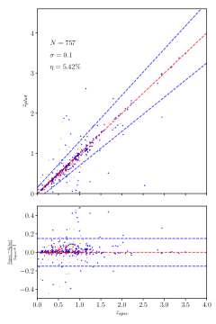
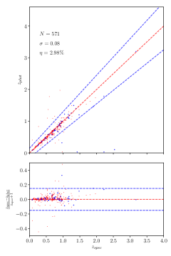
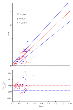
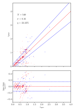
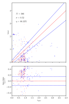
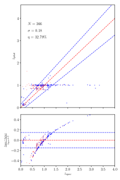
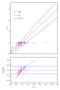
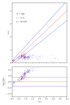
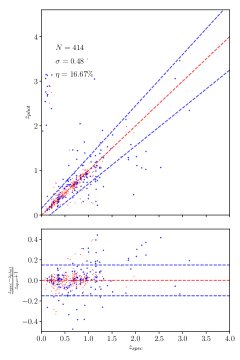
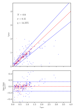
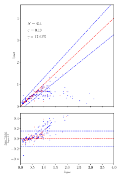
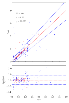
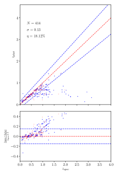
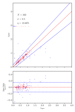
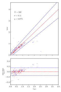
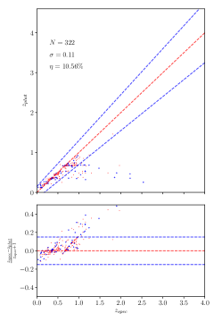
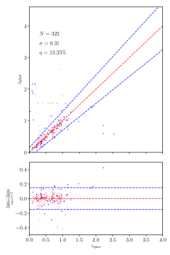
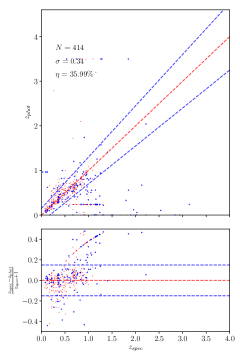
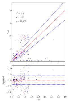
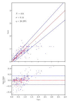
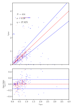
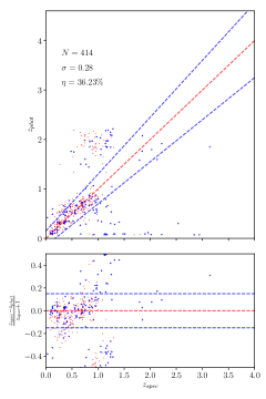
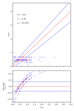
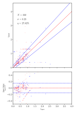
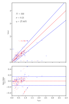
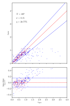
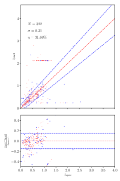
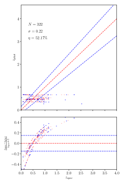
We summarise the results of the tests in Table 3 and present a plot for each test in Figures 2 to 11. We define the error on each measurement , and we define an “outlier” as being a measurement for which . The upper panel of each plot shows the distribution of vs. , and the lower panel shows the normalized residuals vs . The dashed blue lines mark the position of the outlier region defined by . The dashed red line marks the locus of .
In the Table we list: the number of points used in the test set; = standard deviation ; the normalised median absolute deviation = NMAD = ; and the fraction of outliers for which . Because the fraction of outliers does not take into account the reduction in the sample size due to missing or bad data, we also define an overall success rate as the number of correct (i.e. non-outlier) redshifts divided by the total sample size, expressed as a percentage.
In each plot we identify the sources that were classified as AGN on the basis of mid-infrared colours (Chang et al., 2017; Donley et al., 2012), or an X-ray detection by Chandra or XMM.
5.1 Results from the Le Phare experiments
Le Phare does not use a training set, and instead fits the data to astrophysically-derived templates. We therefore ran Le Phare on the entire sample of objects. The templates do not include radio photometry, and thus for none of the experiments with radio=Y we have a result from Le Phare. The results are shown in Figure 2.
Predictably, Le Phare performs better than any of the other techniques when using all available data, but progressively degrades as the quality of the available data is reduced. In particular, when only shallow, broad band photometry is available, systematics appear –photoz constant over a large range of redshift ranges– because the key features such as the 4000Å fall within bands.
5.2 Results from the BRIGHT biased experiments
Experiments A1 to H1 train each algorithm on a brighter data set, then apply it to the full data set. If this were an effective strategy, it would be invaluable to future surveys, since spectroscopy is often not available on fainter objects. However, no supervised machine learning techniques perform well in circumstances in which the training set differs significantly from the test set, and this is reflected in the results shown in Table 3. This experiment demonstrates that, training on a brighter part of the galaxy distribution does not provide enough information for the algorithm to be able to extrapolate to fainter objects. While this result may appear trivial, it is a warning that larger and deeper spectroscopic surveys are essential to train algorithms to measure redshifts for surveys such as EMU . Given the poor quality of the results, we do not show the plots for each experiment, but instead show a representative sample in Figure 3.
5.3 Results on the RANDOM DEEP experiments
As may be expected, compared to their performance on the BRIGHT experiments, the machine learning methods perform better on a randomly selected training set, which matches the test set. Here we summarize the results of these experiments on the RANDOM DEEP experiments, in which the full-depth data in the KB are used.
5.3.1 Experiment A2: RDNY
In this experiment, the full-depth COSMOS data, including X-ray sources, are used, and radio data are not used to train the algorithms. As shown in Fig. 4, all ML methods perform well, with an overall succss rate in the range 82–86%. The best performing overall are kNN and MLPQNA, followed by RF-JHU, which has a smaller fraction of outliers but a slightly larger . kNN performs overall well, but seems to be affected by systematics, with the largest around , presumably because of the paucity of neighbours at high redshift. MLPQNA tends to seriously overestimate the redshift of the very nearby sources.
5.3.2 Experiment B2: RDYY
This experiment (B2) differs from the previous one (A2) only in that the radio data are included in the training set. In most cases the results of B2 are almost indistinguishable from those of A2. For MLPQNA the standard deviation is halved by the inclusion of radio data, bringing back to the correct redshift the sources that in the previous experiment had an overestimated redshift. In most cases, for all the methods, the majority of the outliers are the sources that a posteriori were found to be AGN. We conclude that adding a single radio photometry measurement to an existing excellent optical/IR photometric data set can limit the fraction of high-redshift outliers. At low redshift, UV data can be used for this purpose, but for EMU, the GALEX data available is too shallow to be useful in most cases.
5.3.3 Experiment C2: RDNN
This experiment (C2) differs from A2 in that XMM X-ray sources are excluded from the training and test sets. All methods, with the exception of RF-JHU, had a lower outlier rate on this variation than on A2, but also a lower sample size, resulting in a lower overall success rate. RF-JHU performed similarly in the two experiments, and ended up with a significantly higher success rate than the other methods.
As shown in Fig. 6 the lowest outlier rate , is obtained with MLPQNA, RF-NA and kNN. RF-NA has almost half the fraction of outliers than MLPQNA which shows a systematic pattern at . kNN tends systematically to put the sources at for all the sources above , probably for the same reason discussed in the first experiment.
5.3.4 Experiment D2: RDYN
D2 differs from C2 in that radio fluxes are used in the training process. As shown in Fig. 7, all tests performed very similarly or slightly worse than C2. The lowest outlier rates are achieved by MLPQNA, RF-NA and kNN, whilst RF-JHU assigns the greatest absolute number of non-outlier redshifts because of its lower failure rate. All methods perform poorly at redshifts higher than , where training points become scarce.
5.4 Results on the RANDOM SHALLOW experiments
In the RANDOM SHALLOW experiments, we deliberately degrade the quality of the optical/IR photometric data to simulate the photometric data that will be available for EMU.
5.4.1 Experiment E2: RSNY
In this experiment, the training sample included the XMM detected sources and we used degraded photometry data, without using the Radio data. Naturally the results are not as good as the full-depth data, but the results of E2, shown in Figure 8, still represent a valuable source of redshifts for large radio surveys. The RF-JHU algorithm performs the best, with % outliers and , , but it fails above .
5.4.2 Experiment F2: RSYY
F2 differs from E2 by including radio data. The results, shown in Figure 9, show that all methods have a success rate that is not significantly different from E2, confirming that the addition of a single radio photometric point does not provide useful information.
5.4.3 Experiment G2: RSNN
G2 differs from F2 by excluding radio and X-ray data. The results, shown in Figure 10, show that MLPQNA and RF-JHU outlier rates are improved by omitting these data, although their success rates are lower. Thus, when the photometric data set is poorly sampled, the results will be improved by flagging AGN. For example, flagging all the EMU sources that are detected by eROSITA, will improve the quality of the photometric redshifts for the remaining sources.
5.4.4 Experiment H2: RSYN
H2 differs from G2 by including radio data. Figure 11 shows that MLPQNA has a smaller number of systematic outliers than G2, but a slightly lower overall success rate. In addition RF-JHU and RF-NA improve on the outliers and have a slightly hight overall succss rate than G2. In this experiment the large outliers are mainly the AGN that were unidentified at the time of performing the experiment.
6 Discussion
When given all the available data (experiment A2), Le Phare performed better than any of the ML methods, and performed even better when the X-ray sources were treated separately (C2). Also when the photometry is reduced, its performance are overall superior, but comparable to to RF-JHU in terms of accuracy and fraction of outliers.
In the RANDOM-DEEP experiments (A2 to D2), all algorithms performed quite well (with NMAD -, and -%, compared to - and -%, respectively, for Le Phare), with RF-NA typically performing rather better than the others, and MLPQNA often best at high redshift. However, the high reliability of both MLPQNA and RF-NA are obtained at the cost of reducing the number of sources for which a photometric redshift is provided, resulting in an overall success rate of for MLPQNA and RF-NA, compared with about 80% for RF-JHU. The lack of photoz for about 1/3 of the sources indicate that these sources are not represented by the training sample. kNN generally performed well at low redshifts, but had a greater tendency than the other techniques to fail at , presumably because of the paucity of neighbours at high redshift.
In the RANDOM-SHALLOW experiments (E2 to H2), all algorithms performed less well than with the deeper data (with NMAD -, -%, compared to -% for Le Phare), with RF-NA typically performing rather better than the others. The best performing was RF-JHU and the worst performing was kNN, which essentially failed on these data. Luken et al. (2018) has shown that kNN is capable of good performance on low sensitivity data, and subsequent experiments have shown that that particular implementation of kNN tends to fail on training sets smaller than 100 objects.
Nevertheless, it is encouraging that most methods give useful results even on the shallow data. For example, of the 70 million EMU sources, about 70% are likely to have photometry (from SkyMapper, SDSS, VHS, and WISE) comparable to that used in experiments E2 to H2, and RF-JHU was able to provide redshifts for 80% of these, with an NMAD 0.1. This level of scatter is quite adequate for many of the EMU science goals, and having redshifts for 50% of the EMU sources will significantly enhance the science from EMU.
Nevertheless, it is likely that even better results can be obtained by (i) making full use of the available multi-frequency radio data, and (ii) developing the algorithms further to optimise them for the limited data available for most EMU sources. Further work is continuing (e.g. Luken et al., 2018) to achieve this.
7 Conclusion
We have tested a number of photometric redshift techniques, including both template-fitting and machine learning techniques, on high-quality photometric data in the COSMOS field, and also explored reducing the quality of the photometric data to match that available from all-sky radio surveys such as EMU. We find that:
-
•
Given high-quality multi-band photometry such as is available for the COSMOS data, the template-fitting Le Phare technique outperforms the machine learning techniques tested here, especially when X-ray sources are omitted.
-
•
When the quality of the photometry is reduced to match that available for the EMU all-sky radio survey, both the template-fitting and the machine learning techniques give comparable results, typically with -% of sources appearing as outliers, and with NMAD -.
-
•
Most machine learning techniques perform better at than at higher redshifts, presumably because of the paucity of training data at higher redshifts.
-
•
This level of redshift information from reduced-sensitivity data is still valuable and will result in a significant enhancement to the science from these surveys.
In this first set of experiments, we have set a baseline which will no doubt be improved on by further work in this field. Particularly important future directions are to (i) obtain better training data for radio sources at high redshifts, and (ii) continue developing the algorithms, optimizing them for the lower quality photometry likely to be available, (iii) develop techniques to measure a probability distribution function for the result, rather than a single value, (iv) use measured or estimated uncertainties as a weighting function on the input data, and (v) use the combination of several different techniques to estimate reliability and to detect possible catastrophic failures.
acknowledgments
SC acknowledges support from the project “Quasars at high redshift: physics and cosmology” financed by the ASI/INAF agreement 2017-14-H.0. MB acknowledges the INAF PRIN-SKA 2017 program 1.05.01.88.04 and the funding from MIUR Premiale 2016: MITIC. VS acknowledges support from the European Union’s Seventh Frame-work program under grant agreement 337595 (ERC Starting Grant, “CoSMass”).
| Field | X-ray | UV | OPTICAL | NIR | MIR | Radio |
| Flux | magnitude | magnitude | magnitude | magnitude | Flux | |
| COSMOS | XMM,Chandra | GALEX | 22 bandsa | J,H,K | IRAC band 1 | VLA |
| 25 | 26 | 23.5 | 5 Jy | 10 Jy/bm rms | ||
| EMU | eROSITA | GALEX | Skymapper (5 bands) | VHS (Y,J,H,K) | WISE W1 | EMU |
| 20.4 | 21.5 | 20 | 26 Jy | 10 Jy/bm rms |
| id | parameter | note |
|---|---|---|
| 1 | u_cfht | U photometry from CFHT Megaprime |
| 2 | B_subaru | B photometry from Subaru Suprime-cam |
| 3 | V_subaru | V photometry from Subaru Suprime-cam |
| 4 | g_subaru | G photometry from Subaru Suprime-cam |
| 5 | r_subaru | R photometry from Subaru Suprime-cam |
| 6 | i_subaru | I photometry from Subaru Suprime-cam |
| 7 | z_subaru | Z photometry from Subaru Suprime-cam |
| 8 | J_wfcam | J photometry from UKIRT WFCAM |
| 9 | H_wircam | H photometry from CFHT Wircam |
| 10 | flamingos_Ks | Ks photometry from Gemini FLAMINGOS |
| 11 | K_wircam | K photometry from CFHT Wircam |
| 12 | i_cfht | I photometry from CFHT Megaprime |
| 13 | u_SDSS | u’ photometry from SDSS |
| 14 | g_SDSS | g’ photometry from SDSS |
| 15 | r_SDSS | r’ photometry from SDSS |
| 16 | i_SDSS | i’ photometry from SDSS |
| 17 | z_SDSS | z’ photometry from SDSS |
| 18 | f814 | Subaru Suprime-cam 814nm |
| 19 | IB427 | Subaru Suprime-cam 427nm |
| 20 | IB464 | Subaru Suprime-cam 464nm |
| 21 | IB484 | Subaru Suprime-cam 484nm |
| 22 | IB505 | Subaru Suprime-cam 505nm |
| 23 | IB527 | Subaru Suprime-cam 527nm |
| 24 | IB574 | Subaru Suprime-cam 574nm |
| 25 | IB624 | Subaru Suprime-cam 624nm |
| 26 | IB679 | Subaru Suprime-cam 679nm |
| 27 | IB709 | Subaru Suprime-cam 709nm |
| 28 | IB738 | Subaru Suprime-cam 738nm |
| 29 | IB767 | Subaru Suprime-cam 767nm |
| 30 | IB827 | Subaru Suprime-cam 827nm |
| 31 | NB711 | Subaru Suprime-cam 711nm |
| 32 | NB816 | Subaru Suprime-cam 816nm |
| 33 | ch1 | IRAC band 1 (3.6 m) |
| 34 | ch2 | IRAC band 2 (4.5 m) |
| 35 | ch3 | IRAC band 3 (5.8 m) |
| 36 | ch4 | IRAC band 4 (8.0 m) |
| 37 | galex1500 | Galex 150 nm |
| 38 | galex2500 | Galex 250nm |
| 39 | morphology | See http://irsa.ipac.caltech.edu/data/COSMOS/tables/morphology/ |
| 40 | zspec | spectroscopic redshift |
| 41 | radio_integrated_flux | VLA integrated 20cm radio flux |
| 42 | xmm_soft | XMM soft |
| 43 | xmm_hard | XMM hard |
| 44 | ch_soft | Chandra soft |
| 45 | ch_hard | Chandra hard |
a)
 b)
b)
 c)
c)
 d)
d)
a)
 b)
b)
 c)
c)
 d)
d)
a)
 b)
b)
 c)
c)
 d)
d)
a)
 b)
b)
c)
 d)
d)
a)
 b)
b)
 c)
c)
 d)
d)
a)
 b)
b)
 c)
c)
 d)
d)
a)
 b)
b)
 c)
c)
 d)
d)
a)
 b)
b)
 c)
c)
 d)
d)
a)
 b)
b)
 c)
c)
 d)
d)
a)
 b)
b)
 c)
c)
 d)
d)
References
- Abdalla et al. (2011) Abdalla, F. B., Banerji, M., Lahav, O., & Rashkov, V. 2011, MNRAS, 417, 1891
- Amaro et al. (2017) Amaro, V., Cavuoti, S., Brescia, M., et al. 2017, Astroinformatics, Proc. IAU Symposium, Vol. 325, 197, Cambridge University Press
- Amaro et al. (2018) Amaro, V., Cavuoti, S., Brescia, M., et al. 2018, MNRAS, sty2922, https://doi.org/10.1093/mnras/sty2922
- Aretxaga et al. (2007) Aretxaga, I., Hughes, D. H., Coppin, K., et al. 2007, MNRAS, 379, 1571
- Arnouts et al. (1999) Arnouts, S.; Cristiani, S.; Moscardini, L., Matarrese, S., Lucchin, F. et al., 1999, MNRAS, 310, 540
- Baum (1962) Baum, W. A. 1962, Problems of Extra-Galactic Research, Proc. IAU Symposium15, 390
- Benítez (2000) Benítez, N. 2000, ApJ, 536, 571
- Benítez et al. (2009) Benítez, N., Moles, M., Aguerri, J. A. L., et al. 2009, ApJ, 692, L5
- Bolzonella et al. (2011) Bolzonella, M., Miralles, J.-M., & Pelló, R. 2011, Astrophysics Source Code Library, ascl:1108.010
- Boller et al. (2016) Freyberg, M. J., Trümper, J., Haberl, F., et al. 2016, A&A, 588,103
- Brammer et al. (2010) Brammer, G. B., van Dokkum, P. G., & Coppi, P. 2010, Astrophysics Source Code Library, ascl:1010.052
- Breiman (1984) Breiman, L., Friedman, J. H., Olshen, R. & Stone, C. J. ,1984, Classification and Regression Trees. Belmont, CA: Wadsworth.
- Breiman (1996) Breiman, L. 1996, Machine Learning, Springer Eds., 24, 2, 123-140
- Breiman (2001) Breiman, L., 2001, Machine Learning, Springer Eds., 45, 1, 25-32
- Brescia et al. (2013) Brescia M., Cavuoti S., D’Abrusco R., Mercurio A., Longo G., 2013, ApJ, 772, 140
- Brescia et al. (2014) Brescia, M.; Cavuoti, S.; Longo, G. et al., 2014, PASP, 126, 942, 743-797
- Brescia et al. (2015) Brescia, M.; Cavuoti, S.; Longo, G., De Stefano, V., 2015, A&A, 568, A126, 7 pp.
- Brusa et al. (2010) Brusa, M., Civano, F., Comastri, A., et al. 2010, ApJ, 716, 348
- Budavári & Szalay (2008) Budavári, T., & Szalay, A. S. 2008, ApJ, 679, 301
- Butchins (1981) Butchins, S., 1981, A& A, 97, 407
- Byrd et al. (1994) Byrd R.H., Nocedal J., Schnabel R.B., 1994, Mathematical Programming, 63, 4, pp. 129-156
- Capak et al. (2007) Capak, P., Aussel, H., Ajiki, M., et al. 2007, ApJS, 172, 99
- Carliles et al. (2010) Carliles, S., Budavári, T., Heinis, S., Priebe, C., & Szalay, A. S. 2010, ApJ, 712, 511
- Carrasco et al. (2015) Carrasco, D., Barrientos, L. F., Pichara, K., et al. 2015, A&A, 584, A44
- Cavuoti et al. (2012) Cavuoti S., Brescia M., Longo G., Mercurio A., 2012, A&A, 546, 13
- Cavuoti et al. (2014) Cavuoti S.; Brescia M.; Longo G., 2014, Proc. IAU Symposium, Vol. 306, Cambridge University Press
- Cavuoti et al. (2015a) Cavuoti, S., Brescia, M., Tortora, C., et al. 2015, MNRAS, 452, 3, 3100-3105
- Cavuoti et al. (2015b) Cavuoti S., Brescia M., De Stefano, V., Longo G., 2015, Experimental Astronomy, Springer, Vol. 39, Issue 1, 45-71
- Cavuoti et al. (2017) Cavuoti, S., Amaro, V. Brescia, M., Vellucci, C., Tortora, C., Longo, G., 2017 MNRAS, 465 (2), pp. 1959-1973
- Cavuoti et al. (2017b) Cavuoti, S., Tortora, C., Brescia, M., et al. 2017b, MNRAS, 466 (2), pp. 2039-2053
- Chang et al. (2017) Chang, Y.-Y., Le Floc’h, E., Juneau, S., et al. 2017, ApJS, 233, 19
- Civano et al. (2012) Civano, F., Elvis, M., Brusa, M., et al. 2012, ApJS, 201, 30
- Dahlen et al. (2013) Dahlen, T., Mobasher, B., Faber, S. M., et al. 2013, ApJ, 775, 93
- Delorme et al. (2008) Delorme, P., Willott, C. J., Forveille, T., et al. 2008, A&A, 484 (2), pp. 469-478
- Dark Energy Survey Collaboration et al. (2016) Dark Energy Survey Collaboration, Abbott, T., Abdalla, F. B., et al. 2016, MNRAS, 460, 1270
- D’Isanto et al. (2018) D’Isanto, A., Cavuoti, S., Gieseke, F. and Polsterer, K. L. 2018, A&A, 616, 97
- Donley et al. (2012) Donley, J. L., Koekemoer, A. M., Brusa, M., et al. 2012, ApJ, 748, 142
- Duncan et al. (2018a) Duncan, K. J., Brown, M. J. I., Williams, W. L., et al. 2018a, MNRAS, 473, 2655
- Duncan et al. (2018b) Duncan, K. J., Jarvis, M. J., Brown, M. J. I., & Röttgering, H. J. A. 2018, MNRAS, 477, 5177
- Firth et al. (2002) Firth, A.E., Lahav, O. and Somerville, R. S., 2002, MNRAS
- Fotopoulou et al. (2018) Fotopoulou, S., Paltani, S., 2018, A&A, 619, 14
- Geach (2012) Geach, J. E. 2012, MNRAS, 419, 2633
- Gieseke et al. (2011) Gieseke, F., Polsterer, K. L., Thom, A., et al. 2011, arXiv:1108.4696
- Hasinger et al. (2007) Hasinger, G., Cappelluti, N., Brunner, H., et al. 2007, ApJS, 172, 29
- Hasinger et al. (2018) Hasinger, G., Capak, P., Salvato, M., et al. (2018), ApJ, 858, 77
- Herrera Ruiz et al. (2017) Herrera Ruiz, N., Middelberg, E., Deller, A., et al. 2017, A&A, 607, A132
- Hildebrandt et al. (2010) Hildebrandt, H., Arnouts, S., Capak, P., et al. 2010, A&A, 523, A31
- Hildebrandt et al. (2008) Hildebrandt, H., Wolf, C., & Benítez, N. 2008, A&A, 480, 703
- Ho et al. (1998) Ho, T. K., 1998, IEEE transactions on pattern analysis and machine intelligence, 20. 832-844
- Hsu et al. (2014) Hsu, L.-T., Salvato, M., Nandra, K., et al. 2014, ApJ, 796, 60
- Ilbert et al. (2006) Ilbert, O.; Arnouts, S.; McCracken, H. J.; Bolzonella, M.; Bertin, E et al., 2006, A& A, 457, 841
- Ilbert et al. (2009)
- Ilbert et al. (2009) Ilbert, O., Capak, P., Salvato, M., et al. 2009, ApJ, 690, 1236
- La Franca et al. (2012) La Franca, F., Melini, . G., Bonchi, A., & Fiore, F. 2012, 39th COSPAR Scientific Assembly, 39, 1013
- Laigle et al. (2016) Laigle, C., McCracken, H. J., Ilbert, O., et al. 2016, ApJS, 224, 24
- Loh & Spillar (1986) Loh, E. and Spillar, E.J., 1986, Ap.J., 303, 154
- Lonsdale et al. (2003) Lonsdale, C. J., Smith, H. E., Rowan-Robinson, M., et al. 2003, PASP, 115, 897
- Luken et al. (2018) Luken, K., et al. 2018, PASP, submitted.
- Mao & Urry (2017) Mao, P., & Urry, C. M. 2017, ApJ, 841, 113
- Marchesi et al. (2016) Marchesi, S., Lanzuisi, G., Civano, F., et al. 2016, ApJ, 830, 100
- Masters et al. (2015) Masters, D., Capak P., Stern D., Ilbert O., Salvato M., Schmidt S., Longo G., et al. 2015, ApJ, 813, 1
- McCracken et al. (2010) McCracken, H., Capak, P., Salvato, M., et al. 2010, ApJ, 708, 202
- McMahon et al. (2013) McMahon, R. G., Banerji, M., Gonzalez, E., et al. 2013, The Messenger, 154, 35
- Merloni et al. (2012) Merloni, A., Predehl, P., Becker, W.; Böhringer, H., et al. 2012, arXiv:1209.3114
- Norris et al. (2013) Norris, R. P., et al. 2013, PASA, 30, e020
- Norris et al. (2011) Norris, R. P., Hopkins, A. M., Afonso, J., et al. 2011, PASA, 28, 215
- Norris (2017a) Norris, R. P. 2017a, Astroinformatics, Proc. IAU Symposium, Vol. 325, 103, Cambridge University Press
- Norris (2017b) Norris, R. P. 2017b, Nature Astronomy, 1, 671
- Oyaizu et al. (2008) Oyaizu, H., Lima, M., Cunha, C. E., et al. 2008, ApJ, 674, 768-783
- Pasquet-Itam & Pasquet (2017) Pasquet-Itam, J., & Pasquet, J. 2017, arXiv:1712.02777
- Pearson et al. (2013) Pearson, E. A., Eales, S., Dunne, L., et al. 2013, MNRAS, 435, 2753
- Polsterer et al. (2013) Polsterer, K. L., Zinn, P.-C., & Gieseke, F. 2013, MNRAS, 428, 226
- Polsterer et al. (2014) Polsterer, K. L., Gieseke, F., Igel, C., & Goto, T. 2014, Astronomical Data Analysis Software and Systems XXIII, 485, 425
- Predehl et al. (2007) Predehl, P., Andritschke, R., Bornemann, W., et al. 2007, Proc. SPIE, 6686, 668617
- R Core Team (2013) R Core Team 2013, R: A language and environment for statistical computing. R Foundation for Statistical Computing, Vienna, Austria. ISBN 3-900051-07-0, URL http://www.R-project.org/.
- Rowan-Robinson et al. (2008) Rowan-Robinson, M., Babbedge, T., Oliver, S., et al. 2008, MNRAS, 386, 697
- Salvato et al. (2009) Salvato, M., Hasinger, G., Ilbert, O., et al. 2009, ApJ, 690, 1250
- Salvato et al. (2011) Salvato, M., Ilbert, O., Hasinger, G., et al. 2011, ApJ, 742, 61
- Salvato et al. (2018) Salvato, M., Ilbert, O., & Hoyle, B., 2018, Nature Astronomy, in press.
- Sanders et al. (2007) Sanders, D. B., Salvato, M., Aussel, H., et al. 2007, ApJS, 172, 86
- Santini et al. (2015) Santini, P., Ferguson, H. C., Fontana, A., Mobasher, B., et al. 2015, ApJ, 801, 97
- Sargent et al. (2010) Sargent, M. T., Schinnerer, E., Murphy, E., et al. 2010, ApJS, 186, 341
- Schinnerer et al. (2007) Schinnerer, E., Smolčić, V., Carilli, C. L., et al. 2007, ApJS, 172, 46
- Schinnerer et al. (2010) Schinnerer, E., Sargent, M. T., Bondi, M., et al. 2010, ApJS, 188, 384
- Scoville et al. (2007) Scoville, N., Aussel, H., Brusa, M., et al. 2007, ApJS, 172, 1
- Smolčić et al. (2008) Smolčić, V., Schinnerer, E., Scodeggio, M., et al. 2008, ApJS, 177, 14
- Smolčić et al. (2017) Smolčić, V., Novak, M., Bondi, M., et al. 2017, A&A, 602, A1
- Tagliaferri et al. (2003) Tagliaferri, R., Longo, G., Andreon, S., et al. 2003, Lecture Notes in Computer Science, 2859, 226
- Taniguchi et al. (2007) Taniguchi, Y., Scoville, N., Murayama, T., Sanders, D. B., et al. 2007, ApJS, 172, 9
- Tikhonov et al. (1995) Tikhonov, A. N., Goncharsky, A., Stepanov, V., et al. 1995, Numerical Methods for the Solution of Ill-Posed Problems, Springer Netherlands
- Wolf et al. (2018) Wolf, C., Onken, C. A., Luvaul, L. C., et al. 2018, Publications of the Astronomical Society of Australia, 35, e010.
- Wright et al. (2010) Wright, E. L., Eisenhardt, P. R. M., Mainzer, A. K., et al. 2010, AJ, 140, 1868-1881
- Zamojski et al. (2007) Zamojski, M. A., Schiminovich, D., Rich, R. M., et al. 2007, ApJS, 172, 468
- Zinn et al. (2012) Zinn, P.-C. 2012, Science from the Next Generation Imaging and Spectroscopic Surveys, 52