On the Structure of Time-delay Embedding in Linear Models of Non-linear Dynamical Systems

Abstract

This work addresses fundamental issues related to the structure and conditioning of linear time-delayed models of non-linear dynamics on an attractor. While this approach has been well-studied in the asymptotic sense (e.g. for infinite number of delays), the non-asymptotic setting is not well-understood. First, we show that the minimal time-delays required for perfect signal recovery are solely determined by the sparsity in the Fourier spectrum for scalar systems. For the vector case, we provide a rank test and a geometric interpretation for the necessary and sufficient conditions for the existence of an accurate linear time delayed model. Further, we prove that the output controllability index of a linear system induced by the Fourier spectrum serves as a tight upper bound on the minimal number of time delays required. An explicit expression for the exact linear model in the spectral domain is also provided. From a numerical perspective, the effect of the sampling rate and the number of time delays on numerical conditioning is examined. An upper bound on the condition number is derived, with the implication that conditioning can be improved with additional time delays and/or decreasing sampling rates. Moreover, it is explicitly shown that the underlying dynamics can be accurately recovered using only a partial period of the attractor. Our analysis is first validated in simple periodic and quasi-periodic systems, and sensitivity to noise is also investigated. Finally, issues and practical strategies of choosing time delays in large-scale chaotic systems are discussed and demonstrated on 3D turbulent Rayleigh-Bénard convection.

It is well-known that periodic and quasi-periodic attractors of a non-linear dynamical system can be reconstructed in a discrete sense using time-delay embedding. Following this argument, it has been shown that even chaotic non-linear systems can be represented as a linear system with intermittent forcing. Although it is known that linear models such as those generated by the Hankel Dynamic Mode Decomposition can - in principle - reconstruct an ergodic dynamical system in an asymptotic sense, quantitative details such as the required sampling rate and the number of delays remain unknown. For scalar and vector periodic systems, we derive the minimal necessary time delays and show that time delays not only lead to a more expressive feature space but also result in better numerical conditioning. Further, we explain the reason behind the accurate recovery of attractor dynamics using only a partial period of data. Finally, we discuss the impact of the number of delays in modeling large-scale chaotic systems, e.g., turbulent Rayleigh-Bénard convection.

I Introduction

Time-delay embedding, also known as delay-coordinate embedding, refers to the inclusion of history information in dynamical system models. This idea has been employed in a wide variety of contexts including time series modeling Chen and Billings (1989); Hegger, Kantz, and Schreiber (1999), Koopman operators Arbabi and Mezic (2017); Arbabi and Mezić (2017); Kamb et al. (2018); Brunton et al. (2017) and closure modeling Pan and Duraisamy (2018a). The use of delays to construct a “rich" feature space for geometrical reconstruction of non-linear dynamical systems is justified by the Takens embedding theorem Takens (1981) which states that by using a delay-coordinate map, one can construct a diffeomorphic shadow manifold from univariate observations of the original system in the generic sense, and its extensions in a measure-theoretic sense Sauer, Yorke, and Casdagli (1991), filtered memory Sauer, Yorke, and Casdagli (1991), deterministic/stochastic forcing Stark et al. (2003a, b), and multivariate embeddings Deyle and Sugihara (2011).

Time delay embedding naturally arises in the representation of the evolution of partially observed states in dynamical systems. As an illustrative example, consider a $N$-dimensional linear autonomous discrete dynamical system with $Q$ partially observed (or resolved) states, $Q<N$:

$${}\begin{bmatrix}\mathbf{\hat{x}}^{n+1}\\ \mathbf{\tilde{x}}^{n+1}\end{bmatrix}=\begin{bmatrix}\mathbf{A}_{11}&\mathbf{A}_{12}\\ \mathbf{A}_{21}&\mathbf{A}_{22}\end{bmatrix}\begin{bmatrix}{\color[rgb]{0,0,0}\mathbf{\hat{x}}^{n}}\\ {\color[rgb]{0,0,0}\mathbf{\tilde{x}}^{n}}\end{bmatrix},$$ (1)

where $\mathbf{\hat{x}}^{n}\in\mathbb{R}^{Q}$, $\mathbf{\tilde{x}}^{n}\in\mathbb{R}^{N-Q}$, $n\in\mathbb{N}$, $\mathbf{A}_{11}\in\mathbb{R}^{Q\times Q}$, $\mathbf{A}_{12}\in\mathbb{R}^{Q\times(N-Q)}$, $\mathbf{A}_{21}\in\mathbb{R}^{(N-Q)\times Q}$, $\mathbf{A}_{22}\in\mathbb{R}^{(N-Q)\times(N-Q)}$. The dynamical evolution of the observed states $\mathbf{\hat{x}}$ is given by:

$${}\mathbf{\hat{x}}^{n+1}=\mathbf{A}_{11}\mathbf{\hat{x}}^{n}+\sum_{k=0}^{n-1}\mathbf{A}_{12}\mathbf{A}_{22}^{k}\mathbf{A}_{21}\mathbf{\hat{x}}^{n-1-k}+\mathbf{A}_{12}\mathbf{A}_{22}^{n}\mathbf{\tilde{x}}^{0}.$$ (2)

Typically, the last term is of a transient nature, and thus the above equation can be considered to be closed in the observed variables $\bm{\hat{x}}$. The second term on the right hand side of Equation 2 describes how the time-history of the observed modes affects the dynamics. Thus, Equation 2 implies that it is possible to extract the dynamics of the observables $\mathbf{\hat{x}}$ using time delayed observables, i.e., $\mathbf{\hat{x}}^{n+1}=\mathbf{C}_{0}\mathbf{\hat{x}}^{n}+\sum_{k=1}^{L}\mathbf{C}_{k}\mathbf{\hat{x}}^{n-k}$, where $\mathbf{C}_{k}\in\mathbb{R}^{Q\times Q}$, and $L$ is the number of time delays. It should, however, be noted that explicit delays might not be necessary if one has access to high order time derivatives Takens (1981) or abundant distinct observations Deyle and Sugihara (2011).

Leveraging delay coordinates to construct predictive models of dynamical systems has been a topic of great interest. As an example, such models have been studied extensively in the time series analysis community via the well-known family of autoregressive and moving average (ARMA) models Box et al. (2015). In the machine learning community, related ideas are used in feedforward neural networks (FNN) that augment input dimensions with time delays Frank, Davey, and Hunt (2001), time-delay neural networks (TDNN) Lang, Waibel, and Hinton (1990); Peddinti, Povey, and Khudanpur (2015); Bromley et al. (1994) that statically perform convolutions in time, and the family of recurrent neural networks (RNN) Goodfellow et al. (2016) that dynamically perform non-linear convolutions in time Ma, Wang et al. (2018). In a dynamical systems context, time delays are leveraged in higher order or Hankel Dynamic Mode Decomposition  Le Clainche and Vega (2017a); Arbabi and Mezic (2017); Brunton et al. (2017). Although in essence, each community relies on approximations with time-delays, the focus is typically on different aspects: the time series community focuses on stochastic problems, and prefer explicit and interpretable models Box et al. (2015); the machine learning community is typically more performance-driven and focuses on minimizing the error and scalability Peddinti, Povey, and Khudanpur (2015); the dynamical systems community is focused on the regulated, continuous dynamical system and interpretability of temporal behavior in terms of eigenvalues and eigenvectors Kaiser, Kutz, and Brunton (2018). Moreover, the scientific computing community emphasizes very high dimensional settings, as exemplified by fluid dynamics.

A relevant and outstanding question in each of the aforementioned contexts is the following: Given time series data from a non-linear dynamical system, how much memory is required to accurately recover the underlying dynamics, given a model structure? The memory can be characterized by the two hyperparameters, namely the number of time delays and the corresponding data sampling intervals, if uniformly sampled. Takens embedding theorem Takens (1981) proved the generic existence of a time delayed system with $L=\lceil{2n_{box}}\rceil$ delays, where ($n_{box}$ is box counting dimension of the attractor, given the model has enough non-linearity to approximate the diffeomorphism. However, the question of how to determine the number of time delays and sampling rate is not well-addressed. Given $n_{box}$ as the box counting dimension of the attractor, the number of required time delays $L_{takens}=\lceil{2n_{box}}\rceil$ is rather conservative Gilmore and Lefranc (2003). For example, it is both well known in practice and shown analytically Pan and Duraisamy (2018a), that a typical chaotic Lorenz attractor with box counting dimension $\approx 2.06$ McGuinness (1983) can be well embedded with $L=2$, i.e., an equivalent 3D time delay system, while $L=4$ is required from Takens embedding theorem.

However, other than acknowledging a diffeomorphism, the Takens embedding theorem does not posit any constraints on the mapping from time delay coordinates to the original system state. Clearly, the required number of time delays depends on the richness (non-linearity) of the embedding. In general, for nonlinear models, the determination of the time delays becomes a problem of phase-space reconstruction Frank, Davey, and Hunt (2001); Abarbanel et al. (1993). Popular methods include the false nearest neighbor method Kennel, Brown, and Abarbanel (1992), singular value analysis Broomhead and Jones (1989), averaged mutual information Sugihara, Grenfell, and May (1990), saturation of system invariants Abarbanel et al. (1993), box counting methods Sauer and Yorke (1993), correlation integrals Kim, Eykholt, and Salas (1999), standard model selection techniques Cao (1997), and even reinforcement learning Liu, Ng, and Quek (2007). On the other hand, for linear models, criteria based on statistical significance such as the model utility F-test Lomax and Hahs-Vaughn (2013) or information theoretic techniques such as AIC/BIC Box et al. (2015) are used. The use of the partial autocorrelation in linear autoregressive (AR) models to determine the number of delays can be categorized as a model selection approach. It should be mentioned that by treating the models as a black-box, a general approach such as cross validation can be leveraged.

When the sampling rate is fixed, the question of the number of time delays required should not be confused with the length of statistical dependency between the present and past states on the trajectory. For example, an AR(2) model can have a long time statistical dependency, but the number of time delays in the model may be very small. Indeed, it has been explicitly shown Pan and Duraisamy (2018a) that for a non-linear dynamical system with dual linear structure, embedding the memory in a dynamic fashion requires a much smaller number of delays compared to a prescribed static model structure Gouasmi, Parish, and Duraisamy (2017).

From the viewpoint of discovering the dynamics of a partially observed system, the goal is to determine the non-linear convolution operator Chorin and Hald (2014); Gouasmi, Parish, and Duraisamy (2017) or the so-called closure dynamics Pan and Duraisamy (2018a). It has to be recognized that the number of time delays will also be dependent on the specific structure of the model. The interchangeability between the number of distinct observables and the number of time delays is also reflected in Takens’ original work on the embedding theorem Takens (1981). Such interchangeability with the latent space dimension is also explored in closure dynamics Pan and Duraisamy (2018a); Gouasmi, Parish, and Duraisamy (2017); Parish, Wentland, and Duraisamy (2018) and recurrent neural networks Goodfellow et al. (2016). Since the required number of delays is strongly dependent on the model structure, it is prudent to first narrow down to a specific type of model, and then determine the delays needed.

The connection between time delay embedding and the Koopman operator is elucidated by Brunton et al. Brunton et al. (2017). Further theoretical investigations were conducted by Arbabi and Mezić Arbabi and Mezic (2017). For an ergodic dynamical system, assuming that the observable belongs to a finite-dimensional Koopman invariant subspace $\mathcal{H}$, they showed that Hankel-DMD, a linear model (first proposed and connected to ERA Juang and Pappa (1985)/SSA Vautard, Yiou, and Ghil (1992) by Tu et al. Tu et al. (2014)), can provide an exact representation of the Koopman eigenvalues and eigenfunctions in $\mathcal{H}$. This pioneering work, together with several numerical investigations on the application of Hankel-DMD to non-linear dynamical systems Champion, Brunton, and Kutz (2019); Le Clainche and Vega (2017a); Brunton et al. (2017) and theoretical studies on time-delayed observables using singular value decomposition (SVD) Kamb et al. (2018) highlight the ability of linear time delayed models to represent non-linear dynamics. From a heuristic viewpoint, SVD has been demonstrated Broomhead and Jones (1989); Broomhead and King (1986); Gibson et al. (1992) to serve as a practical guide to determine the required number of time delays and sampling rate, for linear models.

It should be noted that much of the literature Tu et al. (2014); Schmid (2010); Brunton, Proctor, and Kutz (2013) related to DMD and Hankel-DMD consider SVD projection either in the time delayed dimension (e.g. singular spectrum analysis) or the state dimension. SVD can provide optimal linear coordinates to maximize signal-to-noise ratio Gibson et al. (1992), and thus promote robustness and efficiency. On the other hand, projection via Fourier transformation enables the possibility of additional theoretical analysis. For instance, Fourier-based analysis of the Navier–Stokes equations include non-linear triadic wave interactions Pope (2000) and decomposition into solenoidal and dilatational components Pan and Johnsen (2017). Pertinent to the present work, ergodic systems characterized by periodic or quasi-periodic attractors have been shown to be well approximated by Fourier analysis Schilder et al. (2006); Rowley et al. (2009); Mezić (2005). Fourier analysis has also been employed to approximate the transfer function to obtain an intermediate discrete-time reduced order model with stability guarantees for very large scale linear systems Willcox and Megretski (2005); Gugercin and Willcox (2008). For general phase space reconstruction, asymptotic decay rates from Fourier analysis have been leveraged to infer appropriate sampling intervals and number of delays Lipton and Dabke (1996). We thus leverage a Fourier basis representation to uncover the structure of time delay embeddings in linear models of non-linear dynamical systems. We also address related issues of numerical conditioning. It should be emphasized that this work is purely concerned with deterministic linear models and noise free data. It can also be shown that SVD becomes equivalent to Fourier analysis in the limit of large windows Gibson et al. (1992).

The manuscript is organized as follows: The problem formulation and model structure is presented in Section II. Following this, the Fourier transformation of the problem and main theoretical results regarding the minimal time delay embedding for both scalar and vector time series together with explicit, exact solutions of the delay transition matrix after Fourier transformation are presented in Sections III and IV. Modal decompositions related to the Koopman operator is described in Section V. Numerical implementation and theoretical results related to conditioning issues is presented and verified numerically in Section VI, while applications on several nonlinear dynamical systems are displayed in Section VII. The main contributions of the work are summarized in Section VIII.

II Linear model with time-delay embedding

Consider a continuous autonomous dynamical system,

$$\frac{d}{dt}\mathbf{x}=\mathbf{F}(\mathbf{x}(t)),$$ (3)

on a state space $\mathcal{M}\subset\mathbb{R}^{J}$, $J\in\mathbb{N}^{+}$, where $\mathbf{x}$ is the coordinate vector of the state, $\mathbf{x}\in\mathcal{M}$, $\mathbf{F}(\cdot):\mathcal{M}\mapsto\mathbb{R}^{J}$ is in $C^{\infty}$. Denote $\phi_{t}(\mathbf{x}_{0})$, i.e., the flow generated by Equation 3 as the state at time $t$ of the dynamical system that is initialized as $\mathbf{x}(0)=\mathbf{x}_{0}\in\mathcal{M}$. By uniformly sampling with time interval $\Delta t$, the trajectory data of the dynamical systems can be obtained as $\{\mathbf{x}_{j}\}_{j=0}^{\infty}$, where $\mathbf{x}_{j}\triangleq\mathbf{x}(j\Delta t),j\in\mathbb{N}$.

The aforementioned linear model with time-delay embedding order $L$ assumes that the predicted future state $\mathbf{\hat{x}}_{j+1}$ is a sum of $L+1$ linear mappings from the present state $\mathbf{x}_{j}$ and previous $L$ states $\{\mathbf{x}_{j-l}\}_{l=1}^{L}$, $j\in\mathbb{N}$,

$$\mathbf{\hat{x}}_{j+1}=\mathbf{W}_{0}\mathbf{x}_{j}+\mathbf{W}_{1}\mathbf{x}_{j-1}+\ldots+\mathbf{W}_{L}\mathbf{x}_{j-L},$$ (4)

where $\mathbf{W}_{l}\in\mathbb{R}^{J\times J}$ is the associated weight matrix for the $l$-th time-delay snapshot, $l=0,\ldots,L$. As a side note, many data-driven models such as ERA, AR, VAR Box et al. (2015), SSA Vautard, Yiou, and Ghil (1992), HAVOK Brunton et al. (2017), Hankel-DMD Arbabi and Mezic (2017) or HODMD Le Clainche and Vega (2017a), can be derived from the above setup by leveraging impulse response data, introducing stochasticity, analyzing the eigenspectrum on the principal components, or adding intermittent forcing as inputs.

Given $M$ snapshots, the goal is to determine the weight matrices that result in the best possible approximation $\mathbf{\hat{x}}_{j+1}$ to the true future state $\mathbf{x}_{j+1}$ in a priori $L_{2}$ sense, i.e.,

$$\mathbf{W}_{0},\ldots,\mathbf{W}_{L}=\operatorname*{arg\,min}_{\begin{subarray}{c}{\{\mathcal{W}_{i}\}_{i=0}^{L}\in\mathbb{R}^{J\times J}}\end{subarray}}\Bigg{\|}\begin{bmatrix}\mathcal{W}_{L}&\ldots&\mathcal{W}_{0}\end{bmatrix}\begin{bmatrix}\mathbf{x}_{0}&\ldots&\mathbf{x}_{M-2-L}\\ \vdots&\vdots&\vdots\\ \mathbf{x}_{L}&\ldots&\mathbf{x}_{M-2}\end{bmatrix}-\begin{bmatrix}\mathbf{x}_{L+1}&\ldots&\mathbf{x}_{M-1}\end{bmatrix}\Bigg{\|}_{F},$$ (5)

if the minimizer is unique. Otherwise,

$$\mathbf{W}_{0},\ldots,\mathbf{W}_{L}=\operatorname*{arg\,min}_{\begin{subarray}{c}{\mathcal{W}_{0},\ldots,\mathcal{W}_{L}\in\mathbb{R}^{J\times J}}\end{subarray}}\lVert\begin{bmatrix}\mathcal{W}_{L}&\ldots&\mathcal{W}_{0}\end{bmatrix}\rVert_{F},$$ (6)

subject to

$$\begin{bmatrix}\mathcal{W}_{L}&\ldots&\mathcal{W}_{0}\end{bmatrix}\begin{bmatrix}\mathbf{x}_{0}&\ldots&\mathbf{x}_{M-2-L}\\ \vdots&\vdots&\vdots\\ \mathbf{x}_{L}&\ldots&\mathbf{x}_{M-2}\end{bmatrix}=\begin{bmatrix}\mathbf{x}_{L+1}&\ldots&\mathbf{x}_{M-1}\end{bmatrix}.$$

The analytical solution of the above optimization in Equations 5 and 6 is simply the pseudoinverse with SVD Schmid (2010), with trunctation for robustness. However, straightforward SVD computation of the $L$ time-delay matrix for large-scale dynamical systems, e.g., fluid flows $J\sim O(10^{6})$ with $L\sim O(10^{2})$, is challenging. It is therefore prudent to perform spatial truncation using the SVD computed from $\{\mathbf{x}_{j}\}_{j=0}^{M-1}$ that reduces the dimension from $J$ to $r$ ($r\ll J$ and $r\leq\min(J,M)$) and then perform the above optimizations with $L$ time-delays on the $r$-dimensional system Le Clainche and Vega (2017a).

II.1 Illustrative example and simplified consideration for analysis

Consider a scalar non-linear periodic trajectory,

$$x(t)=\cos(t)\sin(\cos(t))+\cos(t/5),$$ (7)

where $t\in[0,40]$. Figure 1 shows the result of a posteriori prediction using a linear model with $L=1$ and $L=12$ trained only on $t\in[0,6]$ with 60 uniform samples. Considering that training data in the above example only covers $[0.6,1.8]$, the prediction of the trajectory over $[-0.9,1.8]$, maybe somewhat surprising. Although the increased expressiveness with time delay embedding have been reported Kutz et al. (2016); Le Clainche and Vega (2017a), reported investigations of the ability of temporal extrapolation are mostly empirical Le Clainche and Vega (2017b); Beltrán, Le Clainche Martinez, and Vega (2018). Note that popular non-linear models, e.g., neural network-based models Pan and Duraisamy (2018b, 2020), despite their property of universal approximation , are trustworthy only within the range of training data. In the present context, this means they are only suitable when training data approximately covers the whole data distribution.

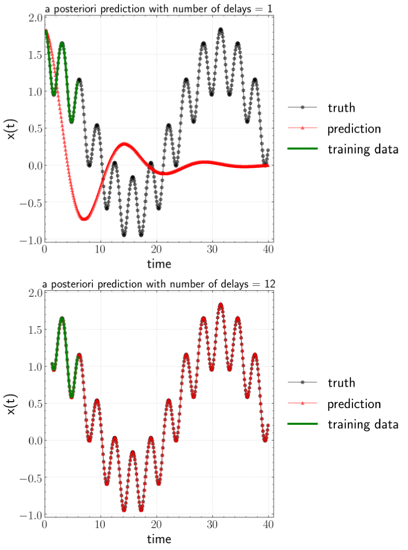
Figure 1: A posteriori prediction on non-linear periodic system with limited training horizon. Top: $L=1$. Bottom: $L=12$.

To provide insight into role of time-delays, we consider the following simplification for the ease of analysis: we restrict ourselves to the dynamics on a periodic attractor, for which one can determine an arbitrarily close Fourier interpolation in time at a uniform sampling rate Attinger, Anne, and McDonald (1966). In addition, without loss of generality, we assume that the data has zero mean, i.e., $\int_{\mathbb{R}^{+}}\mathbf{x}(\tau)d\tau=\mathbf{0}$. We start with the scalar case, and extend the corresponding results to the vector case $\mathbf{x}\in\mathbb{R}^{J}$ in Section IV. Note that the data is collected by uniformly sampling a $T$-periodic time series $x(t)\in\mathbb{R}$. The number of samples per period is $M$, with uniform sampling interval $\Delta t=T/M$. Without loss of generality, we assume that sampling is initiated at $t=0$, $x_{k}=x(t_{k})$, $t_{k}=k\Delta t$, $k\in\mathcal{I}_{M}$, $\mathcal{I}_{M}=\{0,1,\ldots,M-1\}$, and $T$ is the smallest positive real number that represents the periodicity.

II.2 Projection of the trajectory on a Fourier basis

With the simplifications in Section II.1, we consider a surrogate signal of $x(t)$: $S_{M}(t)$

$$S_{M}(t)=\sum_{i\in\mathcal{I}_{M}}a_{i}e^{-j\frac{2\pi it}{T}}\ \ \textrm{with}\ \ a_{i}=\frac{1}{M}\sum_{k\in\mathcal{I}_{M}}x_{k}e^{j\frac{2\pi ki}{M}}\in\mathbb{C},$$ (8)

where $j=\sqrt{-1}$ and

$$\forall k\in\mathcal{I}_{M},\quad x_{k}=x(k\Delta t)=S_{M}(k\Delta t),$$ (9)

which is obtained by projecting $\mathbf{x}(t)$ on the following linear space $\mathcal{H}_{F}$

$$\mathcal{H}_{F}=\operatorname{span}\{1,e^{-j\frac{2\pi t}{T}},\ldots,e^{-j\frac{2\pi(M-1)t}{T}}\},$$ (10)

which is spanned by the Fourier basis in Equation 10 with test functions as delta functions as $\delta(t-t_{k}),k\in\mathcal{I}_{M}$. This process is equivalent to the discrete Fourier transform (DFT).

The above procedure naturally represents the uniformly sampled trajectory in the time domain $\{x_{k}\}_{k=0}^{M-1}$ using coefficients in the frequency domain $\{a_{i}\}_{i=0}^{M-1}$. Since we consider real signals, $\{a_{i}\}_{i=0}^{M-1}$ possess reflective symmetry: $\forall i\in\mathcal{I}_{M}$, $\textrm{Re}(a_{i})=\textrm{Re}(a_{M-i})$, $\textrm{Im}(a_{i})+\textrm{Im}(a_{M-i})=0$, where Re and Im represent the real and imaginary part of a complex number. In addition, since $T$ is the smallest period by definition, we must have $a_{1}=\overline{a_{M-1}}\neq 0$. Further, since $\mathbf{F}$ is smooth, the flow $\phi_{t}(\mathbf{x}_{0})=\mathbf{x}(t)$ is also smooth in $t$ Nijmeijer and Van der Schaft (1990). Thus, the error in the Fourier interpolation is uniformly bounded by twice the sum of the absolute value of truncated Fourier coefficients Boyd (2001). This leads to the uniform convergence

$$\lim_{M\xrightarrow{}\infty}|x(t)-S_{M}(t)|=0.$$ (11)

Hence, one can easily approximate the original periodic trajectory uniformly to the desired level of accuracy by increasing $M$ above a certain threshold.

III The structure of time delay embedding for scalar time series

Now, we apply the linear model with time-delay embedding (Equation 4) at the locations $\{x_{k}\}_{k=0}^{M-1}$. Given $\{x_{k}\}_{k=0}^{M-1}$, consider constructing $L$-time delays of $x(t)$, $L\in\mathbb{N}$. Note that $L=0$ corresponds to no delays considered. To avoid negative indices, we utilize the modulo operation defined in Equation 12,

$$\textrm{$\forall q\in\mathbb{N}$, }\mathcal{P}(q)\triangleq q\ (\mathrm{mod}\ M)=\begin{cases}q,&\text{if }q\in\mathcal{I}_{M},\\ q-M\left\lfloor q/M\right\rfloor,&\text{otherwise}\end{cases}$$ (12)

to construct the $L$ time-delay vector $\mathbf{Y}_{k}$,

$$\mathbf{Y}_{k}=\begin{bmatrix}x_{\mathcal{P}(k)}\\ x_{\mathcal{P}(k-1)}\\ \vdots\\ x_{\mathcal{P}(k-L)}\end{bmatrix}\in\mathbb{R}^{L+1},$$ (13)

where $k\in\mathcal{I}_{M}$, $\left\lfloor\cdot\right\rfloor$ is the floor function. Considering Fourier interpolation, we have

$$\forall q\in\mathcal{I}_{M},\ \ \ \ x_{\mathcal{P}(q)}=\sum_{i\in\mathcal{I}_{M}}a_{i}\omega^{qi},\quad\omega\triangleq e^{-j\frac{2\pi}{M}}\in\mathbb{C},$$ (14)

which is also true for $q\not\in\mathcal{I}_{M}$

$$x_{\mathcal{P}(q)} =S_{M}((q-M\left\lfloor q/M\right\rfloor)\Delta t)=\sum_{i\in\mathcal{I}_{M}}a_{i}e^{-j\frac{2\pi i(q-M\left\lfloor q/M\right\rfloor)}{M}}$$

$$=\sum_{i\in\mathcal{I}_{M}}a_{i}\omega^{qi}.$$ (15)

Using Equation 8, we can rewrite the $L$ time-delay vector $\mathbf{Y}_{k}$ in Equation 13 in the Fourier basis as

$$\mathbf{Y}_{k}=\mathbf{\Omega}_{k,L}\mathbf{a},$$ (16)

where $\forall k\in\mathcal{I}_{M}$, $\mathbf{\Omega}_{k,L}\triangleq\begin{bmatrix}1&\omega^{k}&\omega^{2k}&\ldots&\omega^{(M-1)k}\\ \vdots&\vdots&\vdots&\ddots&\vdots\\ 1&\omega^{k-L}&\omega^{2(k-L)}&\ldots&\omega^{(M-1)(k-L)}\end{bmatrix}$, $\mathbf{a}\triangleq\begin{bmatrix}a_{0}\\ \vdots\\ a_{M-1}\end{bmatrix}\in\mathbb{C}^{M\times 1}$.

The problem of the minimal time delay required for the linear model with $L$ time delays in Equation 4 to perfectly predict the data $\{x_{k}\}_{k=0}^{M-1}$ is equivalent to the existence of the delay transition matrix $\mathbf{K}$ such that,

$$x_{\mathcal{P}(k+1)}=\mathbf{K}^{\top}\mathbf{Y}_{k},\ \ \forall{k}\in\mathcal{I}_{M},$$ (17)

where

$$\mathbf{K}=\begin{bmatrix}K_{0}&K_{1}&\ldots&K_{L}\end{bmatrix}^{\top}\in\mathbb{R}^{(L+1)\times 1},$$

and

$$x_{\mathcal{P}(k+1)}=\mathbf{\Upsilon}_{k}^{\top}\mathbf{a},$$ (18)

where

$$\mathbf{\Upsilon}_{k}\triangleq\begin{bmatrix}1&\omega^{k+1}&\omega^{2(k+1)}&\ldots&\omega^{(M-1)(k+1)}\\ \end{bmatrix}^{\top}.$$ (19)

For convenience, we vertically stack Equation 17 $\forall k\in\mathcal{I}_{M}$,

$$\mathbf{Y}_{M}\mathbf{K}=\mathbf{x}_{M},$$ (20)

where $\mathbf{Y}_{M}\triangleq\begin{bmatrix}\mathbf{Y}_{0}^{\top}\\ \mathbf{Y}_{1}^{\top}\\ \vdots\\ \mathbf{Y}_{M-2}^{\top}\\ \mathbf{Y}_{M-1}^{\top}\end{bmatrix},$ $\mathbf{x}_{M}\triangleq\begin{bmatrix}x_{1}\\ x_{2}\\ \vdots\\ x_{M-1}\\ x_{0}\end{bmatrix}.$

In the following subsections, we discuss the minimal number of required time delays, the exact solution of $\mathbf{K}$ and the number of samples required on the time domain.

III.1 Minimal number of time delays

Our goal is to determine the minimal number of time delays $L$, such that there exists a matrix $\mathbf{K}$ that satisfies the linear system Equation 17. Given one period of data, we can transform the system from the time domain to the spectral domain. Consider Equations 16 and 18, then Equation 20 is equivalent to the following, $\forall{k}\in\mathcal{I}_{M}$:

$$\mathbf{a}^{\top}\left(\begin{bmatrix}1\\ \omega^{k+1}\\ \omega^{2(k+1)}\\ \vdots\\ \omega^{(k+1)(M-1)}\end{bmatrix}-\begin{bmatrix}1&\ldots&1\\ \omega^{k}&\ldots&\omega^{k-L}\\ \omega^{2k}&\ldots&\omega^{2(k-L)}\\ \vdots&\ddots&\vdots\\ \omega^{(M-1)k}&\ldots&\omega^{(M-1)(k-L)}\end{bmatrix}\mathbf{K}\right)=0.$$ (21)

This can be written as

$$\mathbf{a}^{\top}\left(\begin{bmatrix}1&&&&\\ &\omega&&&\\ &&\omega^{2}&&\\ &&&\ddots&\\ &&&&\omega^{(M-1)}\end{bmatrix}^{k}\left(\begin{bmatrix}1\\ \omega\\ \omega^{2}\\ \vdots\\ \omega^{M-1}\end{bmatrix}\\ -\begin{bmatrix}1&\ldots&1\\ 1&\ldots&\omega^{-L}\\ 1&\ldots&\omega^{2(-L)}\\ \vdots&\ddots&\vdots\\ 1&\ldots&\omega^{(M-1)(-L)}\end{bmatrix}\mathbf{K}\right)\right)=0.$$ (22)

We define the residual matrix $\mathbf{R}$ as,

$$\mathbf{R}\triangleq\begin{bmatrix}1\\ \omega\\ \omega^{2}\\ \vdots\\ \omega^{M-1}\end{bmatrix}-\begin{bmatrix}1&1&\ldots&1\\ 1&\omega^{-1}&\ldots&\omega^{-L}\\ 1&\omega^{-2}&\ldots&\omega^{2(-L)}\\ \vdots&\vdots&\ddots&\vdots\\ 1&\omega^{-(M-1)}&\ldots&\omega^{(M-1)(-L)}\end{bmatrix}\mathbf{K}.$$ (23)

Given one period of data, we vertically stack the above equation for each $k\in\mathcal{I}_{M}$. Recognizing the non-singular nature of a Vandermonde square matrix with distinct nodes, we have

$$\begin{bmatrix}a_{0}&a_{1}&a_{2}&\ldots&a_{M-1}\\ a_{0}&\omega a_{1}&\omega^{2}a_{2}&\ldots&\omega^{M-1}a_{M-1}\\ a_{0}&\omega^{2}a_{1}&\omega^{4}a_{2}&\ldots&\omega^{2(M-1)}a_{M-1}\\ \vdots&\vdots&\vdots&\ddots&\vdots\\ a_{0}&\omega^{M-1}a_{1}&\omega^{2(M-1)}a_{2}&\ldots&\omega^{(M-1)(M-1)}a_{M-1}\end{bmatrix}\mathbf{R}=\bm{0}.$$ (24)

This gives

$$\begin{bmatrix}1&1&\ldots&1\\ 1&\omega&\ldots&\omega^{M-1}\\ \vdots&\vdots&\ddots&\vdots\\ 1&\omega^{M-1}&\ldots&\omega^{(M-1)(M-1)}\end{bmatrix}\begin{bmatrix}a_{0}&&&&\\ &a_{1}&&&\\ &&&\ddots&\\ &&&&a_{M-1}\end{bmatrix}\mathbf{R}=\bm{0},$$ (25)

and thus

$$\begin{bmatrix}a_{0}&&&&\\ &a_{1}&&&\\ &&&\ddots&\\ &&&&a_{M-1}\end{bmatrix}\mathbf{R}=\bm{0}.$$ (26)

Note the equivalence between Equation 26 and Equation 20. Now, we consider the case when the Fourier spectrum is sparse with $P$ non-zero coefficients, $P\in\mathbb{N}$ and $P\leq M$. Moreover, it is consistent with the finite point spectral resolution of Koopman operator appears in the laminar unsteady flows Mezić (2013). Denote the set of wave numbers associated with non-zero coefficients as,

$${\mathcal{I}}^{P}_{M}\triangleq\{a_{i}\neq 0|i\in\mathcal{I}_{M}\}=\{i_{p}\}_{p=0}^{P-1},$$ (27)

with ascending order $0\leq i_{0}<i_{1}<\ldots<i_{P-1}\leq M-1$, where $|\hat{\mathcal{I}}^{P}_{M}|=P\in\mathbb{N}$. Note that there is a reflective symmetry restriction on the Fourier spectrum.

The feasibility of using the number of time delays $L$ to ensure the existence of a real solution $\mathbf{K}$ for the linear system is equivalent to the existence of the linear system $\mathbf{R}=\mathbf{0}$ after removing the rows that correspond to zero Fourier modes in $\mathbf{R}$, denoted as $\mathbf{R}_{\mathcal{I}_{M}^{P}}$,

$$\mathbf{R}_{\mathcal{I}_{M}^{P}}=\mathbf{0}\iff\mathbf{A}_{{\mathcal{I}}^{P}_{M},L}\mathbf{K}=\mathbf{b}_{{\mathcal{I}}^{P}_{M}},$$ (28)

where

$$\mathbf{A}_{{\mathcal{I}}^{P}_{M},L}=\begin{bmatrix}1&\omega^{-i_{0}}&\ldots&\omega^{-Li_{0}}\\ 1&\omega^{-i_{1}}&\ldots&\omega^{-Li_{1}}\\ 1&\omega^{-i_{2}}&\ldots&\omega^{-Li_{2}}\\ \vdots&\vdots&\ddots&\vdots\\ 1&\omega^{-i_{P-1}}&\ldots&\omega^{-Li_{P-1}}\\ \end{bmatrix}\in\mathbb{C}^{P\times(L+1)},$$ (29)

and

$$\mathbf{b}_{{\mathcal{I}}^{P}_{M}}=\begin{bmatrix}\omega^{i_{0}}\\ \omega^{i_{1}}\\ \omega^{i_{2}}\\ \vdots\\ \omega^{i_{P-1}}\end{bmatrix}\in\mathbb{C}^{P\times 1}.$$ (30)

Before presenting the main theorem Theorem 1, we define the Vandermonde matrix in Definition 1 and introduce Lemma 1 and Lemma 2.

Definition 1.

Vandermonde matrix with nodes as $\alpha_{0},\alpha_{1},\ldots,\alpha_{M-1}\in\mathbb{C}$ of order $N$ is defined as,

$$\mathbf{V}_{N}(\alpha_{0},\alpha_{1},\ldots,\alpha_{M-1})\triangleq\begin{bmatrix}1&\alpha_{0}&\ldots&\alpha_{0}^{N-1}\\ 1&\alpha_{1}&\ldots&\alpha_{1}^{N-1}\\ \vdots&\vdots&\ddots&\vdots\\ 1&\alpha_{M-1}&\ldots&\alpha_{M-1}^{N-1}\end{bmatrix}.$$

Lemma 1.

$\forall M,N\in\mathbb{N}$, the Vandermonde matrix $\mathbf{A}=\mathbf{V}_{N}(\alpha_{0},\alpha_{1},\ldots,\alpha_{M-1})$ constructed from distinct $\{\alpha_{i}\}_{i\in\mathcal{I}_{M}},\alpha_{i}\in\mathbb{C}$, has the two properties,

1. $\operatorname{rank}(\mathbf{A})=\min(M,N)$,

2. if $\mathbf{A}$ has full column rank, $\forall Q\in\mathbb{N},Q\leq M$, the rank of the submatrix $\mathbf{A^{\prime}}$ by arbitrarily selecting $Q$ rows is $\min(Q,N)$.

Proof.

See Section A.3. ∎

Lemma 2.

$\forall m,n\in\mathbb{N},\mathbf{A}\in\mathbb{R}^{m\times n},\mathbf{b}\in\mathbb{R}^{m\times 1}$, $\exists\mathbf{x}\in\mathbb{C}^{n\times 1}$ s.t. $\mathbf{Ax=b}\iff\exists\mathbf{x}^{\prime}\in\mathbb{R}^{n\times 1}$ s.t. $\mathbf{Ax^{\prime}=b}$. Further, when the solution is unique, the above still holds and the solution is real.

Proof.

See Section A.4. ∎

Theorem 1.

For a uniform sampling of $S_{M}(t)$ with length $M$ and $P$ non-zero coefficients in the Fourier spectrum, the minimal number of time delays $L$ for a perfect prediction, i.e., one that satisfies Equation 20 is $P-1$. Moreover, when $L=P-1$, the solution is unique.

Proof.

See Section A.1. ∎

From the above Theorem 1, we can easily derive Propositions 1 and 2 that are intuitive.

Proposition 1.

If there is only one frequency in the Fourier spectrum of $S_{M}(t)$, simply one time delay in the linear model is enough to perfectly recover the signal.

Proposition 2.

If the Fourier spectrum of $S_{M}(t)$ is dense, then the maximum number of time delays, i.e., over the whole period $M-1$ is necessary to perfectly recover the signal.

In retrospect, the result of the minimal number of time delays for a scalar time series is rather intuitive: any scalar signal with $R$ frequencies corresponds to a certain observable of a $2R$-dimensional linear system. Since more time delays in linear model increases the number of eigenvalues in the corresponding linear system, one requires a minimum of $L=2R-1=P-1$ to match the number of eigenvalues.

III.2 Exact solution for the delay transition matrix $\mathbf{K}$

Two interesting facts have to be brought to the fore:

1. From Equation 28, it is clear that $\mathbf{K}$ is independent of the quantitative value of the Fourier coefficients, but only depends on the pattern in the Fourier spectrum.

2. For $L=P-1$, $\mathbf{A}_{\mathcal{I}_{M}^{P},L}$ is an invertible Vandermonde matrix, which implies the uniqueness of the solution $\mathbf{K}$.

Consider the general explicit formula for the inverse of a Vandermonde matrix Petersen, Pedersen et al. (2008). Note that $\mathbf{A}_{\mathcal{I}_{M}^{P},P-1}=\mathbf{V}_{P}(\omega^{-i_{0}},\ldots,\omega^{-i_{P-1}})$.

Thus

$$\mathbf{A}^{-1}_{\mathcal{I}_{M}^{P},P-1} =\mathbf{V}_{P}^{-1}(\omega^{-i_{0}},\ldots,\omega^{-i_{P-1}}).$$ (31)

$$\mathbf{V}_{P}^{-1}(\omega^{-i_{0}},\ldots,\omega^{-i_{P-1}})_{mn} =(-1)^{m+1}\frac{\displaystyle\sum_{\begin{subarray}{c}0\leq k_{1}<\ldots<k_{P-m}\leq P-1\\ k_{1},\ldots,k_{P-m}\neq n-1\end{subarray}}\omega^{-(i_{k_{1}}+\ldots+i_{k_{P-m}})}}{\displaystyle\prod_{0\leq l\leq P-1,l\neq n-1}\omega^{-i_{l}}-\omega^{-i_{n-1}}}.$$

$$\mathbf{K}_{m} =\mathbf{V}_{P}^{-1}(\omega^{-i_{0}},\ldots,\omega^{-i_{P-1}})_{mn}\mathbf{b}_{\mathcal{I}_{M}^{P},L,n}$$ (32)

$$=\sum_{n=1}^{P}(-1)^{m+1}\frac{\displaystyle\sum_{\begin{subarray}{c}0\leq k_{1}<\ldots<k_{P-m}\leq P-1\\ k_{1},\ldots,k_{P-m}\neq n-1\end{subarray}}\omega^{-(i_{k_{1}}+\ldots+i_{k_{P-m}})}}{\displaystyle\prod_{0\leq l\leq P-1,l\neq n-1}\omega^{-i_{l}}-\omega^{-i_{n-1}}}\omega^{i_{n-1}}$$

$$=\sum_{n=1}^{P}(-1)^{m+1}\frac{\displaystyle\sum_{\begin{subarray}{c}0\leq k_{1}<\ldots<k_{P-m}\leq P-1\end{subarray}}e^{\frac{j2\pi(i_{k_{1}}+\ldots+i_{k_{P-m}})}{M}}}{\displaystyle\prod_{0\leq l\leq P-1,l\neq n-1}e^{\frac{j2\pi{i_{l}}}{M}}-e^{\frac{j2\pi i_{n-1}}{M}}}.$$

where $1\leq m,n\leq P$ and $\mathbf{K}_{m}\equiv K_{m-1}$.

Despite the explicit form, the above expression is not useful in practice. Without loss of generality, considering $P$ is even, the computational complexity at least grows as $\binom{P}{P/2}$. As an example, for a moderate system with 50 non-sparse modes, $\binom{50}{25}\approx 1.2\times 10^{14}$.

III.3 Eigenstructure of the companion matrix

The eigenstructure of the companion matrix formed with time delays is closely related to the Koopman eigenvalues and eigenfunctions under ergodicity assumptions Arbabi and Mezic (2017). From the viewpoint of HAVOK Brunton et al. (2017), for a general time delay $L$, the corresponding Koopman eigenvalues are eigenvalues of the companion matrix $\mathbf{K}_{comp}$ defined as $\mathbf{Y}^{\top}_{k+1}=\mathbf{Y}^{\top}_{k}\mathbf{K}_{comp}$, where

$$\mathbf{K}_{comp}=\begin{bmatrix}K_{0}&1&0&\ldots&0\\ K_{1}&0&1&\ldots&0\\ \vdots&\vdots&\vdots&\ddots&\vdots\\ K_{L-1}&0&0&\ldots&1\\ K_{L}&0&0&\ldots&0\end{bmatrix}\in\mathbb{R}^{(L+1)\times(L+1)}.$$ (33)

The corresponding eigenvalues satisfy $\det(\lambda\mathbf{I}-\mathbf{K}_{comp})=0$, i.e., $\lambda^{L+1}-K_{0}\lambda^{L}-\ldots-K_{L}=0.$ The corresponding eigenstructure is fully determined by the eigenvalues Drmac, Mezic, and Mohr (2019), $\lambda_{0},\ldots,\lambda_{L}$, i.e., $\mathbf{K}_{comp}=\mathbf{Q}^{-1}\mathbf{\Lambda}\mathbf{Q}$, where $\mathbf{\Lambda}=\operatorname{diag}(\lambda_{0},\ldots,\lambda_{L})$, $\mathbf{Q}=\mathbf{V}_{L+1}(\lambda_{0},\ldots,\lambda_{L})$.

III.3.1 Special case: dense Fourier spectrum

Note that $\omega^{-M}=1$ and $P=M$. Consider $L=P-1=M-1$, so that the last column of $A_{\mathcal{I}^{P}_{M},L}$ becomes

$$\begin{bmatrix}1\\ \omega^{-(M-1)}\\ \omega^{-2(M-1)}\\ \vdots\\ \omega^{-(M-1)(M-1))}\end{bmatrix}=\begin{bmatrix}1\\ \omega\\ \omega^{2}\\ \vdots\\ \omega^{M-1}\end{bmatrix}=\mathbf{b}_{\mathcal{I}^{M}_{M}}.$$ (34)

Therefore, the unique solution can be found from observations as

$$\mathbf{K}=\begin{bmatrix}0&\ldots&0&1\end{bmatrix}^{\top}.$$ (35)

The companion matrix Arbabi and Mezic (2017) associated with the Koopman operator is in the form of a special circulant matrix Meyer (2000), for which analytical eigenvalues and eigenvectors can be easily determined. In Equation 33, we have

$$\mathbf{K}_{comp}=\begin{bmatrix}0&1&0&\ldots&0\\ 0&0&1&\ldots&0\\ \vdots&\vdots&\vdots&\ddots&\vdots\\ 0&0&0&\ldots&1\\ 1&0&0&\ldots&0\end{bmatrix}\in\mathbb{R}^{M\times M},$$ (36)

which has eigenvalues evenly distributed on the unit circle

$$\forall i\in\mathcal{I}_{M},\quad\lambda_{i}=e^{-j\frac{2\pi i}{M}}=\omega^{i},$$ (37)

and normalized eigenvectors as

$$\nu_{i}=\frac{1}{\sqrt{M}}\begin{bmatrix}1&\omega^{-i}&\omega^{-2i}&\ldots&\omega^{-(M-1)i}\end{bmatrix}^{\top}.$$ (38)

III.4 Analysis in the time domain

Projection of the trajectory onto a Fourier basis implies that at least one period of training data has to be obtained to be able to construct a linear system that has a unique solution corresponding to $\mathbf{K}^{*}$. However, we will show that in the time domain, a full period of data is not necessary to determine the solution $\mathbf{K}^{*}$ if the Fourier spectrum is sparse.

Denote the number of non-zero Fourier coefficients as $P\in\mathbb{N}$, and its index set as $\mathcal{I}_{M}^{P}$ as before. Instead of having a full period of data, without loss of generality, we consider $L$ time delays and select the $Q$ rows in Equation 20, for which the index is denoted as $0\leq k_{0}<\ldots<k_{Q-1}\leq M-1$, and $Q\in\mathbb{N},L+Q\leq M$. Therefore, we have the following equation in the time domain,

$$\begin{bmatrix}\mathbf{Y}_{k_{0}}^{\top}\\ \mathbf{Y}_{k_{1}}^{\top}\\ \vdots\\ \mathbf{Y}_{k_{Q-2}}^{\top}\\ \mathbf{Y}_{k_{Q-1}}^{\top}\end{bmatrix}\mathbf{K}=\begin{bmatrix}x_{\mathcal{P}(k_{0}+1)}\\ x_{\mathcal{P}(k_{1}+1)}\\ \vdots\\ x_{\mathcal{P}(k_{Q-2}+1)}\\ x_{\mathcal{P}(k_{Q-1}+1)}\end{bmatrix}.$$ (39)

Consider a Fourier transform and recall Equation 22. Choosing $k$ over $k_{0},\ldots,k_{Q-1}$, the above equation can be equivalently rewritten as

$$\begin{bmatrix}a_{0}&\omega^{k_{0}}a_{1}&\omega^{2k_{0}}a_{2}&\ldots&\omega^{(M-1)k_{0}}a_{M-1}\\ a_{0}&\omega^{k_{1}}a_{1}&\omega^{2k_{1}}a_{2}&\ldots&\omega^{(M-1)k_{1}}a_{M-1}\\ a_{0}&\omega^{k_{2}}a_{1}&\omega^{2k_{2}}a_{2}&\ldots&\omega^{(M-1)k_{2}}a_{M-1}\\ \vdots&\vdots&\vdots&\ddots&\vdots\\ a_{0}&\omega^{k_{Q-1}}a_{1}&\omega^{2k_{Q-1}}a_{2}&\ldots&\omega^{(M-1)k_{Q-1}}a_{M-1}\end{bmatrix}\mathbf{R} =\bm{0}.$$ (40)

Recall that only $P$ Fourier coefficients are non-zero, and thus the above equation that constrains $\mathbf{K}$ equivalently becomes

$$\begin{bmatrix}a_{i_{0}}&\omega^{k_{0}}a_{i_{1}}&\omega^{2k_{0}}a_{i_{2}}&\ldots&\omega^{(P-1)k_{0}}a_{i_{P-1}}\\ a_{i_{0}}&\omega^{k_{1}}a_{i_{1}}&\omega^{2k_{1}}a_{i_{2}}&\ldots&\omega^{(P-1)k_{1}}a_{i_{P-1}}\\ a_{i_{0}}&\omega^{k_{2}}a_{i_{1}}&\omega^{2k_{2}}a_{i_{2}}&\ldots&\omega^{(P-1)k_{2}}a_{i_{P-1}}\\ \vdots&\vdots&\vdots&\vdots&\vdots\\ a_{i_{0}}&\omega^{k_{Q-1}}a_{i_{1}}&\omega^{2k_{Q-1}}a_{i_{2}}&\ldots&\omega^{(P-1)k_{Q-1}}a_{i_{P-1}}\end{bmatrix}\mathbf{R}_{\mathcal{I}_{M}^{P}}=\bm{0}$$ (41)

$$\iff\begin{bmatrix}1&\omega^{k_{0}}&\omega^{2k_{0}}&\ldots&\omega^{(P-1)k_{0}}\\ 1&\omega^{k_{1}}&\omega^{2k_{1}}&\ldots&\omega^{(P-1)k_{1}}\\ 1&\omega^{k_{2}}&\omega^{2k_{2}}&\ldots&\omega^{(P-1)k_{2}}\\ \vdots&\vdots&\vdots&\ddots&\vdots\\ 1&\omega^{k_{Q-1}}&\omega^{2k_{Q-1}}&\ldots&\omega^{(P-1)k_{Q-1}}\end{bmatrix}\begin{bmatrix}a_{i_{0}}&&&&\\ &a_{i_{1}}&&&\\ &&a_{i_{2}}&&\\ &&&\ddots&\\ &&&&a_{i_{P-1}}\end{bmatrix}\mathbf{R}_{\mathcal{I}_{M}^{P}}=\bm{0}$$

$$\iff\mathbf{V}_{P}(\omega^{k_{0}},\ldots,\omega^{k_{Q-1}})\operatorname{diag}(a_{i_{0}},\ldots,a_{i_{P-1}})\mathbf{R}_{\mathcal{I}_{M}^{P}}=\mathbf{0}.$$ (42)

Since $\{\omega^{k_{j}}\}_{j=0}^{Q-1}$ are distinct from each other, from Lemma 1, $\textrm{rank}(\mathbf{V}_{P}(\omega^{k_{0}},\ldots,\omega^{k_{Q-1}}))=\min(P,Q)$. Therefore, if we choose to have training data points no less than the number of non-zero Fourier coefficients, i.e., $Q\geq P$, then $\mathbf{V}_{P}(\omega^{k_{0}},\ldots,\omega^{k_{Q-1}})$ is full rank, which leads to $\mathbf{R}_{\mathcal{I}_{M}^{P}}=\mathbf{0}$. Meanwhile, the solution $\mathbf{K}$ is uniquely determined given $L=P-1$. Therefore, given $Q\geq P$,

$$\begin{bmatrix}\mathbf{Y}_{k_{0}}^{\top}\\ \mathbf{Y}_{k_{1}}^{\top}\\ \vdots\\ \mathbf{Y}_{k_{Q-2}}^{\top}\\ \mathbf{Y}_{k_{Q-1}}^{\top}\end{bmatrix}\mathbf{K}=\begin{bmatrix}x_{\mathcal{P}(k_{0}+1)}\\ x_{\mathcal{P}(k_{1}+1)}\\ \vdots\\ x_{\mathcal{P}(k_{Q-2}+1)}\\ x_{\mathcal{P}(k_{Q-1}+1)}\end{bmatrix} \iff\mathbf{R}_{\mathcal{I}_{M}^{P}}=\mathbf{0}{\overset{L=P-1}{\iff}}\textrm{$\mathbf{K}=\mathbf{K}^{*}$}$$ (43)

For the case with minimal number of data samples, i.e., $Q=P$, a natural choice is to construct $P$ rows of the future state from the $P$-th to $2P-1$-th rows in Equation 20. In the above setting, in order to construct the linear system in time domain that has the unique solution $\mathbf{K}^{*}$ of Equation 28, we only require access to the first $2P$ snapshots of data. The key observation is that when the signal is sparse, instead of constructing the classic unitary DFT matrix (Equation 25 to Equation 26), a random choice of $P$ rows will be sufficient to uniquely determine a real solution $\mathbf{K}^{*}$. It has to be mentioned, however, that randomly chosen data points might not be optimal. For example, in Equation 41, the particular choice of sampling (i.e. the choice of $Q$ rows), will determine the condition number of the complex Vandermonde matrix $\mathbf{V}_{P}(\omega^{k_{0}},\ldots,\omega^{k_{Q-1}})$. The necessary and sufficient condition for perfect conditioning of a Vandermonde matrix is when $\{\omega^{k_{j}}\}_{j=0}^{Q-1}$ are uniformly spread on the unit circle Berman and Feuer (2007).

At first glance, our work might appear to be in the same vein as compressed sensing (CS) Donoho (2006); Candes and Tao (2006) where a complete signal is extracted from only a few measurements. However, it should be emphasized that CS requires random projections from the whole field to extract information about a broadband signal in each measurement, while we simply follow the setup in modeling dynamical systems where only deterministic and sequential point measurements are available, and limited to a certain time interval.

Moreover, the above instance of accurately recovering the dynamical system without using a full period of data on the attractor is also reported elsewhere, for instance in sparse polynomial regression for data-driven modeling of dynamical systems Champion, Brunton, and Kutz (2019). Indeed, this is one of the key ideas behind SINDy Brunton, Proctor, and Kutz (2016): one can leverage the prior knowledge of the existence of a sparse representation (for instance, in a basis of monomials), such that sparse regression can significantly reduce the amount of data required with no loss of information.

IV Extension of the analysis to the vector case

In this section, we extend the above analysis to the case of a vector dynamical system. Assuming the state vector has $J$ components, given the time series of $l$-th component, $\{x^{(l)}_{k}\}_{k=0}^{M-1}$, $l=1,\ldots,J$, we have, $\forall k\in\mathcal{I}_{M}$

$$\tilde{x}_{\mathcal{P}(k+1)}=\begin{bmatrix}x_{\mathcal{P}(k+1)}^{(1)}\\ \vdots\\ x_{\mathcal{P}(k+1)}^{(J)}\end{bmatrix}\in\mathbb{R}^{J\times 1},$$ (44)

where $k\in\mathcal{I}_{M},\forall 1\leq l\leq J,l\in\mathbb{N},x^{(l)}_{\mathcal{P}(k)}\in\mathbb{R}$, $J\in\mathbb{N}$. Rewrite Equation 17 in a vector form:

$$\tilde{x}_{\mathcal{P}(k+1)}=\mathbf{\tilde{K}}^{\top}\mathbf{\tilde{Y}}_{k},\ \ \forall{k}\in\mathcal{I}_{M},$$ (45)

where $\tilde{x}_{\mathcal{P}(k+1)}\in\mathbb{R}^{J}$, $\mathbf{\tilde{K}}\in\mathbb{R}^{J(L+1)\times J}$ and

$$\mathbf{\tilde{Y}}_{k}=\begin{bmatrix}\mathbf{Y}^{(1)}_{k}\\ \vdots\\ \mathbf{Y}^{(J)}_{k}\end{bmatrix}\in\mathbb{R}^{J(L+1)\times 1},$$ (46)

where $\mathbf{Y}^{(l)}_{k}$ are the $L$ time-delay embeddings defined in Equation 13 for the $l$-th component of the state. In the present work, we treat the time-delay uniformly across all components.

Following similar procedures as before, denoting the Fourier coefficient of $l$-th component as $\mathbf{a}^{(l)}\in\mathbb{C}^{M\times 1}$, the following lemma which is an analogy to Equation 26 in the scalar case.

Lemma 3.

The necessary and sufficient condition for the existence of a real solution $\mathbf{\tilde{K}}$ in Equation 45 is equivalent to the existence of a solution for the following linear system:

$$\begin{bmatrix}\operatorname{diag}(\mathbf{a}^{(1)})&\ldots&\operatorname{diag}(\mathbf{a}^{(J)})\end{bmatrix}\Bigg{(}\begin{bmatrix}\mathbf{b}_{\mathcal{I}_{M}^{M}}&&\\ &\ddots&\\ &&\mathbf{b}_{\mathcal{I}_{M}^{M}}\end{bmatrix}-$$

$$\begin{bmatrix}\mathbf{A}_{\mathcal{I}_{M}^{M},L}&&\\ &\ddots&\\ &&\mathbf{A}_{\mathcal{I}_{M}^{M},L}\end{bmatrix}\mathbf{\tilde{K}}\Bigg{)}=\mathbf{0}.$$ (47)

The existence of the above solution is equivalent to the following relationship,

$$\operatorname{rank}\left(\begin{bmatrix}\operatorname{diag}(\mathbf{a}^{(1)})\mathbf{A}_{\mathcal{I}_{M}^{M},L}&\ldots&\operatorname{diag}(\mathbf{a}^{(J)})\mathbf{A}_{\mathcal{I}_{M}^{M},L}\end{bmatrix}\right)$$

$$=\operatorname{rank}\left(\begin{bmatrix}\operatorname{diag}(\mathbf{a}^{(1)})\mathbf{A}_{\mathcal{I}_{M}^{M},L}&\ldots&\operatorname{diag}(\mathbf{a}^{(J)})\mathbf{A}_{\mathcal{I}_{M}^{M},L}&\operatorname{diag}(\mathbf{a}^{(1)})\mathbf{b}_{\mathcal{I}_{M}^{M}}&\ldots&\operatorname{diag}(\mathbf{a}^{(J)})\mathbf{b}_{\mathcal{I}_{M}^{M}}\end{bmatrix}\right).$$ (48)

Proof.

See Section A.5. ∎

Next, with the introduction of the Krylov subspace in Definition 2 which frequently appears in the early literatures of DMD Rowley et al. (2009); Schmid (2010), we present Remark 1 and Remark 2 from Lemma 3 that interprets and reveals the possibility of using less embeddings than the corresponding sufficient condition for the scalar case in Theorem 1.

Definition 2 (Krylov subspace).

For $n,r\in\mathbb{N}$, $\mathbf{A}\in\mathbb{C}^{n\times n}$, $\mathbf{b}\in\mathbb{C}^{n\times 1}$, Krylov subspace is defined as

$$\mathcal{K}_{r}(\mathbf{A},\mathbf{b})=\operatorname{span}\{\mathbf{b},\mathbf{Ab},\ldots,\mathbf{A}^{r-1}\mathbf{b}\}.$$ (49)

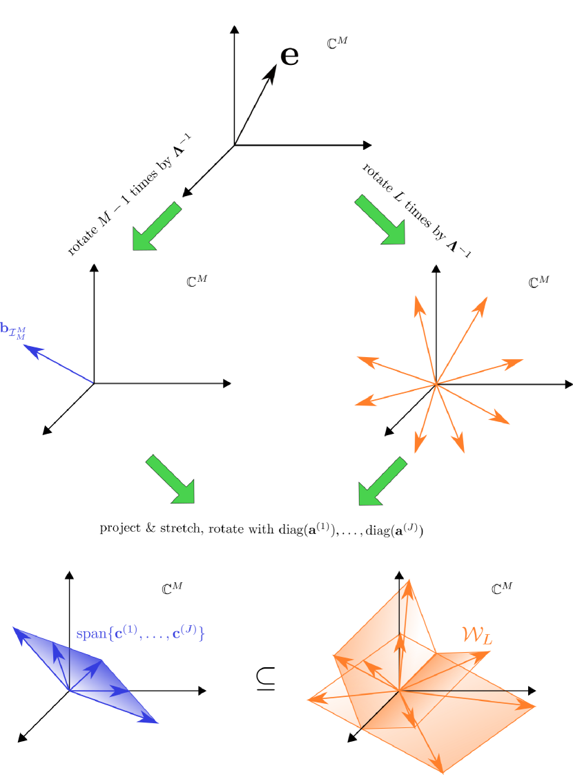
Figure 2: Illustration of the geometrical interpretation of Lemma 3.

Remark 1 (Geometric interpretation).

For $j=1,\ldots,J$, define $\mathbf{c}^{(j)}\triangleq\operatorname{diag}(\mathbf{a}^{(j)})\mathbf{b}_{\mathcal{I}_{M}^{M}}$, and $\mathcal{E}_{L}^{(j)}$ as the column space of $\operatorname{diag}(\mathbf{a}^{(j)})\mathbf{A}_{\mathcal{I}_{M}^{M},L}$. The existence of the solution in Lemma 3 is then equivalent to

$$\forall j\in\{1,\ldots,J\},\mathbf{c}^{(j)}\in\mathcal{W}_{L}\triangleq\mathcal{E}_{L}^{(1)}\oplus\ldots\oplus\mathcal{E}_{L}^{(J)}$$

$$\iff\operatorname{span}{\{\mathbf{c}^{(1)},\ldots,\mathbf{c}^{(J)}\}}\subseteq\mathcal{W}_{L},$$ (50)

where $\mathcal{W}_{L}$ is the column space from all components, and $\oplus$ is the direct sum operation between vector spaces. Note that the column space of $\mathbf{A}_{\mathcal{I}_{M}^{M},L}$ can represented as a Krylov subspace $\mathcal{K}_{L+1}(\mathbf{\Lambda}^{-1},\mathbf{e})$, where

$$\mathbf{e}\triangleq\begin{bmatrix}1&\ldots&1\end{bmatrix}^{\top},$$ (51)

$$\mathbf{\Lambda}\triangleq\operatorname{diag}(\omega^{0},\ldots,\omega^{M-1}).$$ (52)

A geometric interpretation of the above expressions is shown in Figure 2: for each $j$, $\mathbf{b}_{\mathcal{I}_{M}^{M}}=\mathbf{\Lambda}^{-(M-1)}\mathbf{e}$ and $\mathbf{e}$ are projected, stretched and rotated using the $j$-th Fourier spectrum diagonal matrix $\operatorname{diag}(\mathbf{a}^{(j)})$ yields $\mathcal{E}_{L}^{(j)}$ and its total column subspace $\mathcal{W}_{L}$. If all of the projected and stretched $\mathbf{b}_{M}$’s are contained in $\mathcal{W}_{L}$, a real solution exists for Equation 45. Notice that in Equation 50, $\forall i\neq j$, $\mathcal{E}_{L}^{(i)}$ expands the column space $\mathcal{E}_{L}^{(j)}$ to include $\mathbf{c}^{(j)}$. Thus, the minimal number of time delays required in the vector case as in Equation 45 can be smaller than that of the scalar case.

Remark 2 (Interplay between Fourier spectra).

The vector case involves the interaction between the $J$ different Fourier spectra corresponding to each component of the state. This complicates the derivation of an explicit result for the minimal number of time delays as in the scalar case (Theorem 1). We note two important observations that illustrate the impact of the interplay between the $J$ Fourier spectra:

• To ensure $\mathbf{c}^{(j)}$ lies in $\mathcal{W}_{L}$, each $\mathcal{E}_{L}^{(j)}$ should provide distinct vectors to maximize the dimension of $\mathcal{W}_{L}$. If a linear dependency is present in $\{\mathbf{a}^{(j)}\}_{j=1}^{J}$, Equation 50 no longer holds.

• Since $\mathbf{c}^{(j)}$ is projected using $\operatorname{diag}(\mathbf{a}^{(j)})$, if $\mathbf{a}^{(i)\top}\mathbf{a}^{(j)}=0$, $\mathcal{E}_{L}^{(i)}$ will not contribute to increasing the dimension of $\mathcal{W}_{L}$.

Drawing insight from the representation of the column space of $\mathbf{A}_{\mathcal{I}_{M}^{M},L}$ as the Krylov subspace in Remark 1, we present a connection between the output controllability from linear system control theory Kreindler and Sarachik (1964), and the number of time delays required for linear models in a general sense.

Definition 3 (Output controllability).

Consider a linear system with state vector $\mathbf{x}(t)\in\mathbb{C}^{M\times 1}$, $M\in\mathbb{N}$, $t\in\mathbb{R}^{+}$,

$$\dot{\mathbf{x}} =\mathbf{A}\mathbf{x}+\mathbf{B}\mathbf{u},$$ (53)

$$\mathbf{y} =\mathbf{Cx}+\mathbf{Du},$$ (54)

where $\mathbf{A}\in\mathbb{C}^{M\times M}$, $\mathbf{B}\in\mathbb{C}^{M\times N}$, $\mathbf{C}\in\mathbb{C}^{P\times M}$, $\mathbf{D}\in\mathbb{C}^{P\times N}$. $\mathbf{y}(t)\in\mathbb{C}^{P\times 1}$ is the output vector. The above system is said to be output controllable if for any $\mathbf{y}(0),\mathbf{y}^{\prime}\in\mathbb{C}^{P\times 1}$, there exists $t_{1}\in\mathbb{R}^{+},t_{1}<+\infty$ and $\mathbf{u}^{\prime}\in\mathbb{C}^{N\times 1}$, such that under such input and initial conditions, the output vector of the linear system can be transferred from $\mathbf{y}(0)$ to $\mathbf{y}^{\prime}=\mathbf{y}(t_{1})$.

Recall that the necessary and sufficient condition Kreindler and Sarachik (1964); Gruyitch (2018) for a linear system to be output controllable is given in Definition 4. A natural definition for the output controllability index that is similar to the controllability and observability index is given in Definition 5. We summarize the conclusion in Theorem 2 that the output controllability index minus one is a tight upper bound for the number of time delays required for the linear model in the general sense. We again emphasize that the particular linear system with input and output in Theorem 2 is solely induced by the Fourier spectrum of the nonlinear dynamical system on the attractor.

Definition 4 (Output controllability test).

The system in Equations 53 and 54 is output controllable if and only if $\mathcal{OC}(\mathbf{A,B,C,D};M)\triangleq\begin{bmatrix}\mathbf{CB}&\mathbf{CAB}&\ldots&\mathbf{CA}^{M-1}\mathbf{B}&\mathbf{D}\end{bmatrix}$ is full rank. Note that when $\mathbf{D}=\mathbf{0}$, we omit $\mathbf{D}$ in the notation.

Definition 5 (Output controllability index).

If the system in Equations 53 and 54 is output controllable, then the output controllability index is defined as the least integer $\mu$ such that $\mathcal{OC}(\mathbf{A,B,C,D};\mu)\in\mathbb{C}^{P\times(\mu+1)N}$ is full rank.

Lemma 4.

For any matrix $\mathbf{A}$ that is a horizontal stack of diagonal matrices, the row elimination matrix $\mathbf{E}$ that removes any row that is a zero vector leads to a full rank matrix with the rank of original matrix. Moreover, $\mathbf{E^{\top}EA}=\mathbf{A}$.

Proof.

See Section A.6. ∎

Theorem 2.

Following definitions in Equations 51 and 52, consider the following induced linear dynamical system with output controllability index $\mu$:

$$\dot{\mathbf{Z}} =\mathbf{A}\mathbf{Z}+\mathbf{Bu}$$

$$\mathbf{y} =\mathbf{CZ}$$

with

$$\mathbf{A}=\begin{bmatrix}\mathbf{\Lambda}^{-1}&&\\ &\ddots&\\ &&\mathbf{\Lambda}^{-1}\end{bmatrix}\in\mathbb{C}^{MJ\times MJ},$$

$$\mathbf{B}=\begin{bmatrix}\mathbf{e}&&\\ &\ddots&\\ &&\mathbf{e}\end{bmatrix}\in\mathbb{C}^{MJ\times J},$$

$$\mathbf{C}^{\prime}=\begin{bmatrix}\operatorname{diag}(\mathbf{a}^{(1)})&\ldots&\operatorname{diag}(\mathbf{a}^{(J)})\end{bmatrix}\in\mathbb{C}^{M\times JM},$$

$$\mathbf{C}=\mathbf{EC^{\prime}}\in\mathbb{C}^{P\times JM},$$

where $P$ is the number of non-zero row vectors in $\mathbb{C}^{\prime}$, and $\operatorname{rank}\left(\mathbf{C}\right)=\operatorname{rank}\left(\mathbf{C}^{\prime}\right)=P$ as indicated by Lemma 4. Then, $\mu-1$ is a tight upper bound on the minimal number of time delays that ensures the existence of solution of Lemma 3, and thus a perfect reconstruction of the dynamics.

Proof.

See Section A.2. ∎

V Dynamic mode decomposition of a linear model with time-delays

As indicated earlier, the trajectory predicted by linear models with time-delay can be viewed as an observable from an associated high dimensional linear system. To see this, consider a uniformly sampled trajectory data of length $M$, $\{\mathbf{x}_{j}\}_{j=0}^{M-1}$. The $L$ time-delay vector for a $J$-dimensional nonlinear system $\mathbf{x}\in\mathbb{R}^{J}$ is defined as,

$$\mathbf{h}_{k}=\begin{bmatrix}\mathbf{x}_{k-L}\\ \vdots\\ \mathbf{x}_{k}\end{bmatrix},\quad L\leq k\leq M-1.$$ (55)

If the trajectory data can be well approximated by a linear model with $L$ time-delays of the form in Equation 4, then one has the so-called high order dynamic mode decomposition Brunton et al. (2017); Le Clainche and Vega (2017a) for $L\leq k\leq M-2$,

$$\mathbf{h}_{k+1} \approx\mathbf{A}_{L}\mathbf{h}_{k},$$ (56)

$$\mathbf{x}_{k+1}=\mathbf{E}_{L}\mathbf{h}_{k+1} \approx\mathbf{E}_{L}\mathbf{A}_{L}\mathbf{h}_{k}=\mathbf{W}_{L}\mathbf{x}_{k-L}+\ldots+\mathbf{W}_{0}\mathbf{x}_{k}$$ (57)

$$\mathbf{x}_{k+1}=\mathbf{E}_{L}\mathbf{h}_{k+1} \approx\mathbf{E}_{L}\mathbf{A}_{L}^{k+1-L}\mathbf{h}_{L}=\mathbf{Q}_{L}\mathbf{\Lambda}^{k+1-L}\mathbf{P}_{L}$$ (58)

$$\mathbf{x}_{k+1} \approx\sum\nolimits_{i=1}^{J(L+1)}\lambda_{i}^{k+1-L}\mathbf{q}_{i}\mathbf{p}^{\top}_{i}\mathbf{h}_{L}$$ (59)

where $\mathbf{E}_{L}\triangleq\begin{bmatrix}\mathbf{0}&\ldots&\mathbf{0}&\mathbf{I}\end{bmatrix}\in\mathbb{R}^{J\times J(L+1)}$, and $\mathbf{A}_{L}\in\mathbb{R}^{J(L+1)\times J(L+1)}$ is known as the block companion matrix,

$$\mathbf{A}_{L}=\begin{bmatrix}&\mathbf{I}&&&\\ &&\mathbf{I}&&\\ &&&\ddots&\\ &&&&\mathbf{I}\\ \mathbf{W}_{L}&\mathbf{W}_{L-1}&\mathbf{W}_{L-2}&\ldots&\mathbf{W}_{0}\end{bmatrix}=\mathbf{P}_{L}\mathbf{\Lambda}_{L}\mathbf{P}_{L}^{-1},$$ (60)

and

$$\mathbf{P}_{L}^{-1}\triangleq\begin{bmatrix}\mathbf{p}^{\top}_{1}\\ \vdots\\ \mathbf{p}^{\top}_{J(L+1)}\end{bmatrix},\quad\mathbf{Q}_{L}\triangleq\mathbf{E}_{L}\mathbf{P}_{L}=\begin{bmatrix}\mathbf{q}_{1}&\ldots&\mathbf{q}_{J(L+1)}\end{bmatrix}.$$ (61)

Note that the above decomposition in Equation 59 reduces to the standard DMD when $L=0$, i.e.,

$$\mathbf{x}_{k+1}=\sum\nolimits_{i=1}^{J}\lambda_{i}^{k+1-L}\mathbf{q}_{i}\mathbf{p}^{\top}_{i}\mathbf{x}_{0},\quad\forall L\leq k\leq M-2,$$ (62)

where $\mathbf{q}_{i}$ and $\{\lambda_{i}^{k+1-L}\mathbf{p}^{\top}_{i}\mathbf{x}_{0}\}_{k=0}^{M-2}$ are sometimes referred to as the $i$-th spatial modes and temporal modes respectively. With more time-delays $L$, the maximal number of linear waves in the model increases with $J(L+1)$. As a side note, the above modal decomposition can be interpreted as an approximation to the Koopman mode decomposition on the trajectory with $L$ time-delays as observables Brunton et al. (2017); Arbabi and Mezic (2017); Arbabi and Mezić (2017).

VI Verification and practical consideration

In this section, we start with a simple example and discuss practical numerical considerations.

VI.1 5-mode sine signal

First, an explicit time series consisting of five frequencies with a long period $T=100$ is considered:

$$x(t) =0.3\cos(\frac{2\pi t}{100})+0.5\sin(\frac{4\pi t}{100})+0.9\cos(\frac{8\pi t}{100})$$

$$+1.6\sin(\frac{16\pi t}{100})+1.2\cos(\frac{24\pi t}{100}).$$ (63)

Such a signal may be realized, for instance, by observing the first component of a 10-dimensional linear dynamical system. The sampling rate is set at 1 per unit time, which is arbitrary and considered for convenience, and the signal is sampled for two periods from $n=0$ to $n=199$. Thus we have a discretely sampled time series of length 200 as $\{x_{n}\}_{n=0}^{199}$ with $x_{n}=x(t)|_{t=n}$. Only the first 20% of the original signal is used, which is 40% of a full period with around 20 to 30 data points sampled. The variation in the number of data points is due to the fact that we fix the use of first 20% of trajectory, and then reconstruct the signal with a different number of time delays. We solve the least squares problem in the time domain with the iterative least squares solver scipy.linalg.lstsq Jones, Oliphant, and Peterson (2014) with lapack driver as gelsd, and cutoff for small singular values as $10^{-15}$.

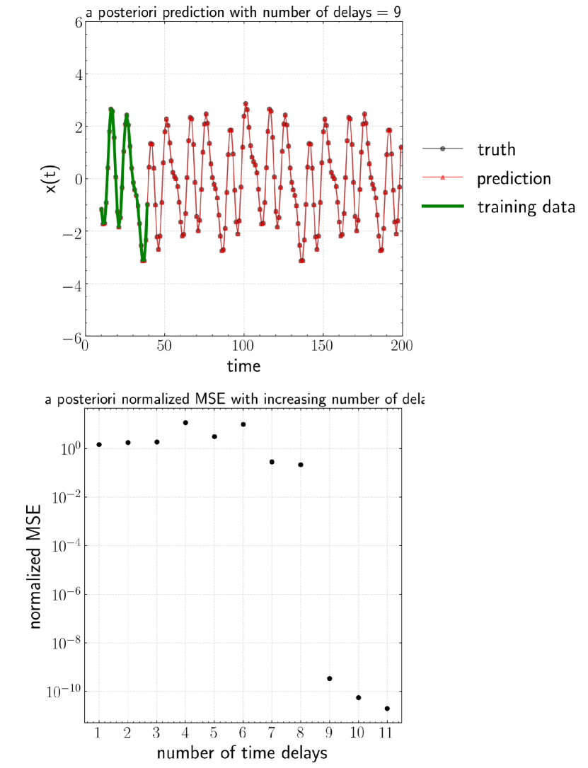
Figure 3: Top: A posteriori prediction vs ground truth, time delayed linear model with number of delays $L=9$. Bottom: A posteriori MSE normalized by standard deviation of $x(t)$ vs number of time delays.

The analysis in Theorem 1 implies that one can avoid using the full period of data for exact prediction. Numerical results are presented in Figure 3 with number of time delays $L=9$. These results show that time delayed DMD, unlike non-linear models such as neural networks, avoid the requirement of a full period of data when the dynamics is expressible by a set of sparse harmonics. From Theorem 1, the 5-mode signal has $P=10$ non-zero Fourier coefficients in the Fourier spectrum, and thus the least number of delays is $L=P-1=9$, which agrees well with Figure 3 which shows the a posteriori mean square error normalized by the standard deviation of the data , between prediction and ground truth. Figure 3 clearly shows that a sharp decrease of a posteriori error when the number of delays $L=9$.

Now we will consider a different scenario. As explained earlier, linear time delayed models can avoid the use of a full period of data if there is enough information to determine the solution within the first $P$ states. Thus, if one increases the sampling rate, less data will be required to recover an accurate solution. However, one still needs to numerically compute the solution of a linear system, while the condition number grows with increasing sampling rates. As displayed in Figure 5, the condition number increases in both time and spectral domain formulations, with increasing sampling rate.

Using scipy.linalg.lstsq Jones, Oliphant, and Peterson (2014) and a time domain formulation, we found that there is no visual difference between the truth and a posteriori prediction when the condition number is below $10^{13}$, i.e., $M\leq 300$ in the spectral domain, or $M\leq 200$ in the time domain. However, as the condition number grows beyond $10^{13}$ (i.e. machine precision noise of even $10^{-16}$ can contaminate digits around 0.001), a posteriori prediction error can accumulate when $M=400$ (Figure 4).

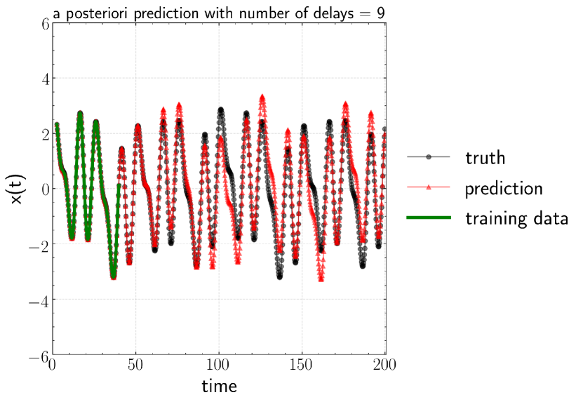
Figure 4: Prediction vs ground truth when sampling rate is excessive, e.g., $M=400$

VI.2 Numerical considerations

In practical terms, one can pursue two general formulations to numerically compute the delay transition matrix $\mathbf{K}$ in Equation 5:

1. Formulation in time domain: If all available delay vectors and corresponding future states are stacked, the direct solution of Equation 5 is a least square problem in the time domain with the requirement of at least $P$ samples.

2. Formulation in spectral domain: In this approach, the Fourier signals from a full period of data is extracted and Equation 28 is numerically solved.

VI.2.1 Ill-conditioning due to excessive sampling rate

Consider signals that consist of a finite number of harmonics with the index set of Fourier coefficients as $\mathcal{I}_{M}^{P}$. Since the first half of the indices $i_{0},\ldots,i_{P/2-1}$ is determined by the inherent period of each harmonic, these indices are independent of the number of samples per period $M$, as long as $M$ satisfies the Nyquist condition. It is thus tempting to choose a relatively large sampling rate. However, this may not be favorable from a numerical standpoint. When $L=P-1$ and the sampling rate is excessive compared to the potentially lower frequency dynamics of the system, each column could become nearly linearly dependent. We will now explore the circumstances under which the corresponding linear system in either the spectral or time domain can become ill-conditioned. It has to also be recognized that the denominator in Equation 32 consists of the difference between different nodes on the unit circle, and can therefore impact numerical accuracy.

The condition number of the Vandermonde matrix with complex nodes Equation 28 is also pertinent to the present discussion. It is well known that the condition number of a Vandermonde matrix grows exponentially with the order of matrix $n$ when the nodes are real positive or symmetrically distributed with respect to the origin Córdova, Gautschi, and Ruscheweyh (1990). When the nodes are complex, the numerical conditioning of a Vandermonde matrix can be as perfect as that of a DFT matrix, or as poor as that of the quasi-cyclic sequence Gautschi (1990). Specifically, it has been shown that a large square Vandermonde matrix is ill-conditioned unless its nodes are nearly uniformly spaced on or about the unit circle Pan (2016). Interestingly, for a rectangular Vandermonde matrix with $n$ nodes and order $N$, i.e., $\mathbf{V}_{N}(z_{1},\ldots,z_{n})$, Kunis and Nagel Kunis and Nagel (2018) provided a lower bound on the 2-norm condition number of the Vandermonde matrix that contains “nearly-colliding" nodes:

$$\kappa_{2}(\mathbf{V}_{N}(z_{1},\ldots,z_{n}))\geq\frac{\sqrt{6}}{\pi\tau}\approx\frac{0.77}{\tau},$$ (64)

for all $\tau\leq 1$, i.e., “nearly colliding", where $\tau\triangleq N\min_{j\neq l}|t_{j}-t_{l}|_{\mathbb{T}}$, $|t_{j}-t_{l}|_{\mathbb{T}}\triangleq\min_{r\in\mathbb{Z}}|t_{j}-t_{l}+r|$. Applying the above result to Equation 28, when $M$ is large enough so that $\tau\leq 1$ is satisfied, the lower bound of the 2-norm condition number will increase proportionally with the number of samples per period $M$. Thus, the tightly clustered nodes due to excessive sampling will lead to the ill-conditioning of the linear system in Equation 28.

VI.2.2 Sub-sampling within Nyquist limits

Equation 64 shows that the tight clustering of nodes due to excessive sampling can lead to ill-conditioning. A straightforward fix would thus be to filter out unimportant harmonics, and re-sample the signal at a smaller sampling rate that can still capture the highest frequency retained in the filtering process. In this way, the nodes can be more favorably redistributed on the unit circle. Recall that, if the complex nodes of the Vandermonde matrix are uniformly distributed on a unit circle, then one arrives at a perfect conditioning of the Vandermonde matrix with condition number of one similar to the DFT matrix Pan (2016). Without any loss of generality, we assume the number of samples per period $M$ is even. The wave numbers of sparse Fourier coefficients are denoted by $\mathcal{I}_{M}^{P}$. The sorted wave numbers are symmetrical with respect to $M/2$ and recall that the values of the first half of $\mathcal{I}_{M}^{P}$, i.e., $i_{0},\ldots,i_{\frac{P}{2}-1}$ is independent of $M$, as long as the Nyquist condition is satisfied Landau (1967). Then, a continuous signal $x(t)$ is sub-sampled uniformly. Due to symmetry, the smallest number of samples per period $M^{*}$ that preserves the signal is $2(i_{\frac{P}{2}-1}+1)$.

VI.2.3 Effect of sampling rate, formulation domain, and numerical solver on model accuracy

To compare the impact of different solution techniques, we choose several off-the-shelf numerical methods to compute $\mathbf{K}$ in either the time domain or spectral domain. These methods include:

(i) mldivide from MATLAB MATLAB (2010), i.e., backslash operator which effectively uses QR/LU solver in our case;

(ii) scipy.linalg.lstsq Jones, Oliphant, and Peterson (2014), which by default calls gelsd from LAPACK Anderson et al. (1999) to solve the minimum 2-norm least squares solution with SVD, and an algorithm based on divide and conquer;

(iii) Björck & Pereyra (BP) algorithm Björck and Pereyra (1970) which is designed to solve the Vandermonde system exactly in an efficient way exploiting the inherent structure. For a $n\times n$ matrix, instead of the standard Gaussian elimination with $O(n^{3})$ arithmetic operations and $O(n^{2})$ elements for storage, the BP algorithm only requires $n(n+1)(2O_{M}+3O_{A})/2$ for arithmetic operations and no further storage than storing the roots and right hand side of the system.

As shown in Figure 5, the condition number increases exponentially with increasing number of samples per period $M$, leading to a significant deterioration of accuracy. Comparing the time and spectral domain formulations, Figure 5 shows that the solution for the spectral case is more accurate than the time domain solution when the sampling rate is low. This is not unexpected as one would need to perform FFT on a full period of data to find the appropriate Fourier coefficients in the spectral case. When $M>600$, however, the spectral domain solutions obtained by BP and mldivide algorithms blow up, while the time domain solution is more robust in that the error is bounded. Note that the singular value decomposition - in lstsq and in mldivide that removes the components of the solution in the subspace spanned by less significant right singular vectors - is extremely sensitive to noise. Further, from Equation 41, the difference between the formulations in the spectral and time domains can be attributed to $\mathbf{V}_{P}(\omega^{k_{0}},\ldots,\omega^{k_{Q-1}})$ and $\operatorname{diag}(a_{i_{0}},\ldots,a_{i_{P-1}})$, which could be ill-conditioned. Thus, regularization in the time domain formulation is more effective. Figure 5 also shows that, when the system becomes highly ill-conditioned, i.e., $M>600$, lstsq with thresholding $\epsilon=10^{-15}$ results in a more stable solution than mldivide.

It should be mentioned that the condition number computed in Figure 5 around the inverse of machine precision, i.e., $O(10^{16})$, should be viewed in a qualitative rather than quantitative sense Drmac, Mezic, and Mohr (2019).

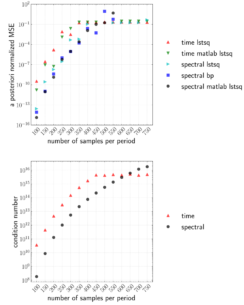
Figure 5: Top: A posteriori MSE normalized by the standard deviation of $x(t)$ with increasing sampling rate and different numerical solvers. Bottom: Numerical condition number with increasing sampling rate

VI.2.4 Effect of the number of time delays $L$ on condition number

By adding more time delays than the theoretical minimum, the dimension of the solution space grows, along with the features for least squares fitting. Accordingly, the null space becomes more dominant, and thus one should expect non-unique solutions with lower residuals. Note that, for simplicity, the following numerical analysis assumes the scalar case, i.e., $J=1$.

For the complex Vandermonde system in Equation 28, following Bazán’s work Bazán (2000), we discovered very distinct features of the asymptotic behavior of the solution, and the corresponding system in Equation 28 when the number of time delays $L\rightarrow\infty$.

(i) The norm of the minimum 2-norm solution of Equation 28 $\lVert\mathbf{\hat{K}}_{L}\rVert_{2}\rightarrow 0$ , as shown in Proposition 3.

(ii) An upper bound for the convergence rate of $\lVert\mathbf{\hat{K}}_{L}\rVert_{2}^{2}$ is derived in Lemma 5.

(iii) An upper bound on the 2-norm condition number of Equation 28 is shown in Proposition 4 to scale with $1+O(1/\sqrt{L})$.

Proposition 3.

$\displaystyle\lim_{L\rightarrow\infty}\lVert\mathbf{\hat{K}}_{L}\rVert_{2}=0$, where $\mathbf{\hat{K}}_{L}$ is the minimum 2-norm solution of Equation 28.

Proof.

See Section A.8. ∎

Lemma 5.

$\forall L\geq P-1$, denote $\mathbf{\hat{K}}_{L}$ as the minimum 2-norm solution of Equation 28. The following tight upper bound can be derived

$$\lVert\mathbf{\hat{K}}_{L}\rVert_{2}^{2}\leq\frac{\lVert\mathbf{\hat{K}}_{P-1}\rVert_{2}^{2}}{1+\left\lfloor{\frac{L-P+1}{M}}\right\rfloor}.$$ (65)

Proof.

See Section A.7. ∎

Proposition 4.

Let $P$ be the number of non-zero Fourier coefficients. $\forall L\geq P-1$, denote $\mathbf{\hat{K}}_{P-1}$ as the unique solution of Equation 28. With the minimal number of time delays, the upper bound on the 2-norm condition number of the system is given by

$$\kappa_{2}(\mathbf{A}_{\mathcal{I}_{M}^{P},L}) =\kappa_{2}(\mathbf{V}_{L+1}(\omega^{-i_{0}},\ldots,\omega^{-i_{P-1}}))$$

$$\leq 1+\frac{d}{2}\left[1+\sqrt{1+\frac{4}{d}}\right],$$ (66)

where

$$d \triangleq P\left[\left(1+\frac{\lVert\mathbf{\hat{K}}_{P-1}\rVert_{2}^{2}}{(P-1)({1+\left\lfloor{\frac{L-P+1}{M}}\right\rfloor})\delta^{2}}\right)^{\frac{P-1}{2}}-1\right],$$ (67)

$$\displaystyle\delta \triangleq\min_{0\leq j<k\leq P-1}|\omega^{-i_{j}}-\omega^{-i_{k}}|.$$ (68)

Further, if $L\rightarrow\infty$, then $\kappa_{2}(\mathbf{A}_{\mathcal{I}_{M}^{P},L})\rightarrow 1$, i.e., perfect conditioning is achieved.

Proof.

See Section A.9. ∎

Remark 3.

Note that the bound in Proposition 4 does not demand a potentially restrictive condition on the number of time delays, i.e., $L+1>2(P-1)/\delta$ that is required in Bazán’s work, which utilizes the Gershgorin circle theorem for the upper bound of the 2-norm condition number Bazán (2000). More recently, this constraint has been defined in the context of the nodes being “well-separated" Kunis and Nagel (2018). Applying such a result to our case, we have

$$\kappa_{2}(\mathbf{A}_{\mathcal{I}_{M}^{P},L})\leq\sqrt{1+\frac{2}{\frac{\delta(L+1)}{2P-2}-1}}$$ (69)

since we have an estimation for the convergence rate of the minimal 2-norm solution. However, although our upper bound in Proposition 4 holds for all $L\geq P-1$, it is too conservative compared to Bazán’s upper bound when $L\rightarrow\infty$. To see this, denote $k_{m}\triangleq\min_{i,j\in\mathcal{I}_{M}^{P},i,\neq j}\{|k||k=(i-j)\bmod{M}\}$, i.e., the minimal absolute difference between any pair of distinct indices in $\mathcal{I}^{P}_{M}$, in the sense of modulo $M$. Assuming that the number of samples per period is large enough so that $M\gg 2\pi k_{m}$, we have $\delta=\sqrt{2\left[1-\cos(2\pi k_{m}/M)\right]}\approx 2\pi k_{m}/M=O(1/M)$. If we assume that the system with time delay $L$ is far from being perfectly conditioned, we have $\kappa_{F}(\mathbf{V}_{L+1})\gg P+2$, which leads to the following approximation for our upper bound,

$$\kappa_{2}(\mathbf{V}_{N})\leq\frac{1}{2}\Big{[}\kappa_{F}(\mathbf{V}_{L+1})-P+2$$

$$+\sqrt{(\kappa_{F}(\mathbf{V}_{L+1})-P+2)^{2}-4}\Big{]}\approx\kappa_{F}(\mathbf{V}_{L+1})-P+2$$

$$\leq d+2.$$ (70)

Hence, for an excessively sampled case, if $L$ is small enough such that $\kappa_{F}(\mathbf{V}_{L+1})\geq\kappa_{2}(\mathbf{V}_{L+1})\gg P+2$ holds but large enough such that

$$\frac{\lVert\mathbf{\hat{K}}_{P-1}\rVert_{2}^{2}}{(P-1)({1+\left\lfloor{\frac{L-P+1}{M}}\right\rfloor})\delta^{2}}\ll 1,$$ (71)

then the approximated upper bound becomes

$$2+d=2+P\left[\left(1+\frac{\lVert\mathbf{\hat{K}}_{P-1}\rVert_{2}^{2}}{(P-1)({1+\left\lfloor{\frac{L-P+1}{M}}\right\rfloor})\delta^{2}}\right)^{\frac{P-1}{2}}-1\right],$$

$$\approx 2+\frac{P\lVert\mathbf{\hat{K}}_{P-1}\rVert_{2}^{2}}{2\delta^{2}({1+\left\lfloor{\frac{L-P+1}{M}}\right\rfloor})}\approx 2+\frac{P\lVert\mathbf{\hat{K}}_{P-1}\rVert_{2}^{2}}{8\pi^{2}k_{m}^{2}/M^{2}({1+\left\lfloor{\frac{L-P+1}{M}}\right\rfloor})}$$

$$=2+O\left(\frac{M^{3}}{L}\right).$$ (72)

Meanwhile, when $L$ is very large, and thus $\delta(L+1)>2(P-1)$ is satisfied, Bazán’s bound in Equation 69 scales with $1+O\left(\sqrt{M}/\sqrt{L}\right)$ for $L/M\gg 1$. Thus, to retain the same upper bound of condition number, one only needs to increase the number of time delays at the same same rate as the sampling.

Figure 6 shows that the residuals from the least squares problem in both the time and spectral domains decrease exponentially with the addition of time delays. Further, the a posteriori MSE shows significant improvement with the addition of time delays.

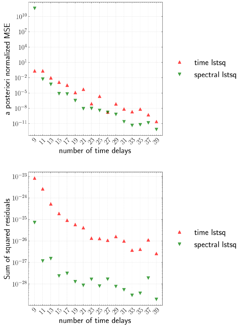
Figure 6: Effect of time delay $L$ on $M=500$ oversampling case. Top: A posteriori MSE normalized by standard deviation of $x(t)$ with increasing time delays. Bottom: Sum of squared residuals with increasing time delays.

Figure 7 shows the trend of the 2-norm condition number in both the time and spectral domains. The condition number decays exponentially in the spectral case, but increases in the time domain case. This appears to be contradictory since the condition number is typically reflective of the quality of the solution. However, since SVD regularization is implicit in scipy.linalg.lstsq with gelsd option, computing the 2-norm condition number in the same way as in the numerical solver, i.e., effective condition number  is a more relevant measure of the quality of the solution of the SVD truncated system. Thus, the reasons for improved predictive accuracy are due to a) the increasing dimension of the solution space for a potentially under-determined system with more time delays, and b) the well conditioned system after SVD truncation as shown in Figure 7. The large condition number in the time domain with increasing number of delays is a result of the ill-conditioning of $\mathbf{V}_{P}(\omega^{k_{0}},\ldots,\omega^{k_{Q-1}})$ and $\operatorname{diag}(a_{i_{0}},\ldots,a_{i_{P-1}})$ in Equation 42.

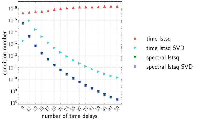
Figure 7: $M=500$ oversampling case: effective condition number decreases with increasing time delay $L$

VI.2.5 Effect of subsampling on model performance

As indicated in Remark 3, reducing the number of samples per period $M$ is shown to decrease the upper bound on the condition number. For a given signal, however, there is a restriction on the minimum possible $M$ compared to the number of time delays $L$. In the above case for the 5-mode sine signal, $i_{\frac{P}{2}-1}=12$, and thus the minimal sampling per period that one can use to perfectly preserve the original signal in the subsampling is $M=26$. The condition number with $M$ ranging from $26$ to $98$ is shown in Figure 8. This shows the effectiveness of subsampling in reducing the condition number significantly. Correspondingly, the a posteriori normalized MSE is also reduced as shown in Figure 8.

The previous two subsections demonstrated the role of numerical conditioning on model performance. We note that explicit stabilization techniques Le Clainche and Vega (2017a); Champion, Brunton, and Kutz (2019) require further investigation.

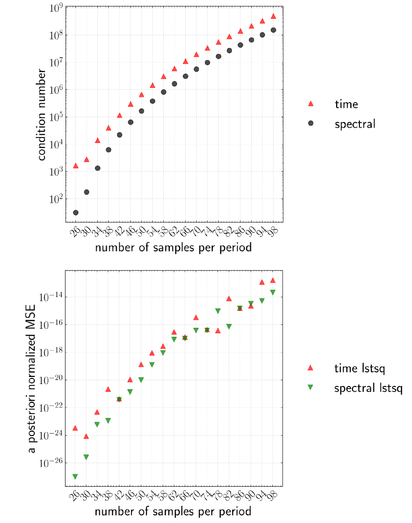
Figure 8: Top: Condition number as a function of sampling rate. Bottom: A posteriori normalized MSE with sampling rate.

VI.3 Issues in large-scale chaotic dynamical systems

Lnear time delayed models have been investigated for chaotic dynamics on an attractor (for instance,  Brunton et al. (2017)). The main challenges are two fold: a) Chaotic systems may require an infinite number of waves to resolve the continuous Koopman spectrum Mezić (2005), and b) Practical chaotic systems of interest in science and engineering science are large-scale. For example, realistic fluid flow simulations, may be very large even after dimension reduction, especially for advection-dominated problems Lee and Carlberg (2020). This would further limit the expressiveness of linear models with time delay.

To illustrate this, consider dimension reduction using SVD on the trajectory data $\{\mathbf{x}_{j}\}_{j=0}^{M-1}$. One can extract a reduced $r$-dimensional trajectory, $\{\hat{\mathbf{x}}_{j}\}_{j=0}^{M-1}$, i.e.,

$$\begin{bmatrix}\mathbf{x}_{0}&\ldots&\mathbf{x}_{M-1}\end{bmatrix}\approx\mathbf{U}_{r}\mathbf{\Sigma}_{r}\mathbf{V}_{r}^{\top},\quad\hat{\mathbf{x}}_{j}=\mathbf{U}_{r}^{\top}\mathbf{x}_{j}\in\mathbb{R}^{r}.$$ (73)

Recalling Equations 5 and 6, we have a similar analytic SVD-DMD solution on the time delay data matrix of the reduced $r$-dimensional system, i.e.,

$$\widehat{\mathbf{A}}_{L}=\mathbf{Q}_{r^{{}^{\prime}}}^{\top}\mathbf{U}_{r}^{\top}\begin{bmatrix}\mathbf{h}_{L+1}&\ldots&\mathbf{h}_{M-1}\end{bmatrix}\mathbf{Z}_{r^{{}^{\prime}}}\mathbf{\Sigma}_{r^{{}^{\prime}}}^{-1}\in\mathbb{R}^{r^{{}^{\prime}}\times r^{{}^{\prime}}},$$ (74)

with the following $r^{{}^{\prime}}-$SVD regularization purely for numerical robustness

$$\mathbf{U}_{r}^{\top}\begin{bmatrix}\mathbf{h}_{L}&\ldots&\mathbf{h}_{M-2}\end{bmatrix}\approx\mathbf{Q}_{r^{{}^{\prime}}}\mathbf{\Sigma}_{r^{{}^{\prime}}}\mathbf{Z}_{r^{{}^{\prime}}}^{\top}.$$ (75)

Note that ${\mathbf{A}}_{L}=\mathbf{Q}_{r^{{}^{\prime}}}\widehat{\mathbf{A}}_{L}\mathbf{Q}_{r^{{}^{\prime}}}^{\top}\in\mathbb{R}^{r(L+1)\times r(L+1)}$ with $\operatorname{rank}({\mathbf{A}}_{L})=r^{{}^{\prime}}$. Following the notations of the mode decomposition in Section V, we have

$$\mathbf{x}_{k+1}\approx\sum\nolimits_{i=1}^{r^{{}^{\prime}}}\lambda_{i}^{k+1-L}\mathbf{U}_{r}\mathbf{q}_{i}\mathbf{p}^{\top}_{i}\mathbf{h}_{L},$$ (76)

where $\mathbf{U}_{r}\mathbf{q}_{i}$ and $\{\lambda_{i}^{k+1-L}\mathbf{p}^{\top}_{i}\mathbf{h}_{L}\}_{k=0}^{M-2}$ are the spatial and temporal modes respectively.

Now we can describe the constraints on the maximal number of modes in the linear model $r^{{}^{\prime}}$ from the time delay $L$. From the restrictions on matrix rank, we have

$$r\leq\min\{J,M\},\quad r^{{}^{\prime}}\leq\min\{r(L+1),M-1-L\},$$ (77)

as illustrated in Figure 9. Clearly, we see the maximal number of waves $r^{{}^{\prime}}$ stops increasing after the time delay $L$ surpasses the intersection point where $L_{*}=\frac{M}{r+1}-1$, $r^{{}^{\prime}}_{*}=\frac{r}{r+1}M$. This relation indicates that keeping more POD modes in the dimension reduction increases the upper limit of the number of waves in the resulting linear models. The corresponding time delay would decrease with respect to the peak. Interestingly, for $L>\frac{M}{r+1}-1$, called “overdelay", might yield an underdetermined linear system as in Equation 6. For example, we can choose $L_{opt}=\lceil{\frac{M}{r+1}}\rceil$. The solution of that system would, however, result in a least square residual near machine precision, leading to overfitting even in a posteriori sense. Note that practical problems may require denoising on the trajectory data.

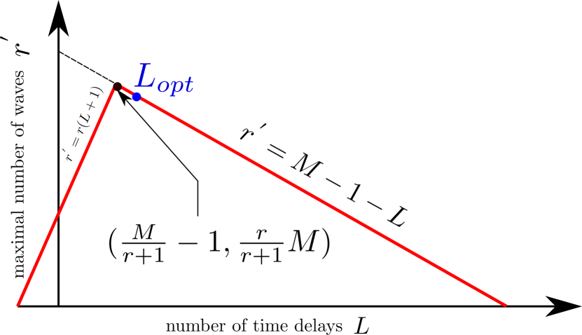
Figure 9: Constraints on maximal number of waves $r^{{}^{\prime}}$ in the linear model with time delays.

VII Applications

VII.1 Van der Pol oscillator

Now we consider the Van der Pol oscillator (VdP) with forward Euler time discretization:

$${}\begin{bmatrix}x^{n+1}_{1}\\ x^{n+1}_{2}\end{bmatrix}=\begin{bmatrix}x^{n}_{1}\\ x^{n}_{2}\end{bmatrix}+\Delta t\begin{bmatrix}x^{n}_{2}\\ \mu(1-x_{1}^{n}x_{1}^{n})x_{2}^{n}-x_{1}^{n}\end{bmatrix},$$ (78)

where $\mu=2$, $x_{1}^{0}=1$, $x_{2}^{0}=0$, $\Delta t=0.01$. After 530 time steps, the system approximately falls on the attractor with an approximate period of 776 steps. Total data is collected after the system falls on the attractor for 4 periods.

As shown in Figure 10, Fourier spectrum for each component of VdP system shows that the exhibition of an approximate sparse spectrum with $P=10$ and $P=18$ for $x_{1}$ and $x_{2}$ respectively. As indicated from Theorem 1, the corresponding time delay and minimal sampling rate is summarized in Table 1.

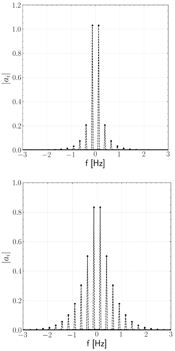
Figure 10: Fourier spectrum for VdP system. Top: $x_{1}$. Bottom $x_{2}$.

Table 1: Summary of the structure of time delay embedding for VdP.

	$P$	$L$	$i_{P/2-1}$	$M_{min}$
$\tilde{x}_{1}(t)$	10	9	9	20
$\tilde{x}_{2}(t)$	18	17	18	38
$\tilde{x}_{1,2}(t)$		8		38

VII.1.1 Prediction of the VdP system without a full period of data: scalar case

From Table 1, it is clear that the smallest number of samples per period is significantly smaller than the original number of samples per period, i.e., $M=776$. The analysis in the previous section also showed that the choice of a smaller number of samples per period is helpful in reducing the condition number. Thus, we choose a moderately subsampled representation without any loss in reconstruction compared to the filtered representation. Individually treating the first and second components, we choose $M=200,100$ with theoretical minimum time delays $L=9,17$, respectively.

Numerical results displayed in Figure 11 show that, even using training data that covers less than 25% of the period for the first component, and 50% of the period for the first component, the linear model with minimal time delays is still able to accurately predict the dynamics over the entire time period of the limit cycle. Note that a similar predictive performance is expected for the original (unfiltered) VdP system.

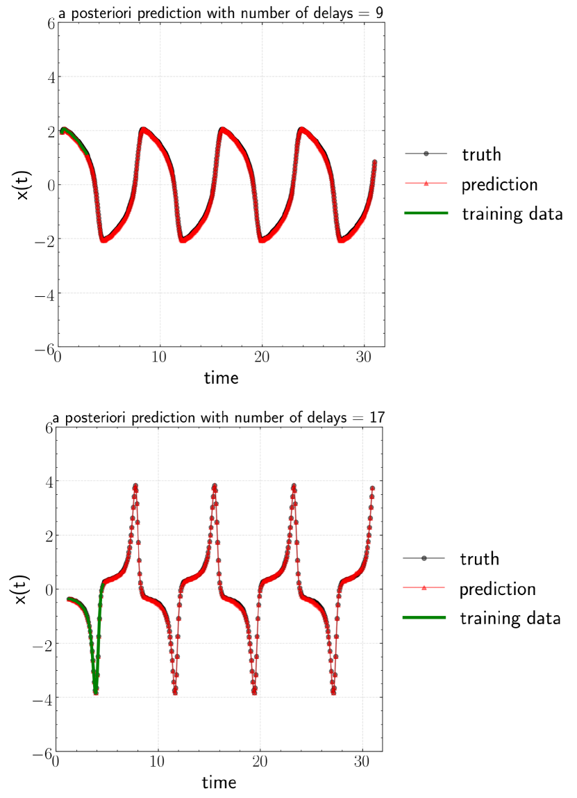
Figure 11: Prediction vs ground truth for each component of VdP. Top: first component. Bottom: second component.

VII.1.2 Prediction of VdP system without a full period of data: vector case

As given in Table 1, Lemma 3 predicts that the consideration of both components requires only 8 delays. The effectiveness of the criterion developed in Lemma 3 is confirmed to a resounding degree in Figure 12. The top figure shows the predictive performance of the time delayed linear model for the minimum number of delays and the bottom figure shows the behavior of the a posteriori normalized MSE versus the number of time delays. It should be recognized that in contrast to the scalar case, in which the minimal time delay can be directly inferred from the Fourier spectrum, the vector case requires iterative evaluations of the rank test in Lemma 3.

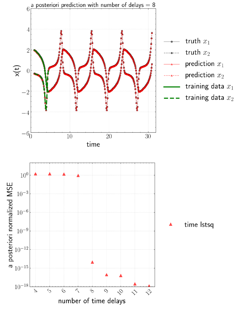
Figure 12: Top: Prediction vs ground truth with $M=80$ for VdP system. Bottom: A posteriori MSE normalized by standard deviation with as a function of the number of time delays for the vector case.

VII.2 Quasi-periodic signal

As indicated in Laudau’s route to chaos Landau (1944), quasi-periodic systems play an important role in the transition from a limit cycle to fully chaotic flow.We consider the following quasi-periodic signal

$$x(t)=\cos(\sqrt{2}t/2)\sin(\sqrt{3}t/2)\cos(t),$$ (79)

where $t\in[0,40]$. Consider a sampling interval $\Delta t=0.1$, we consider the linear model trained on the first 60 snapshots, i.e., $t\in[0,6]$.

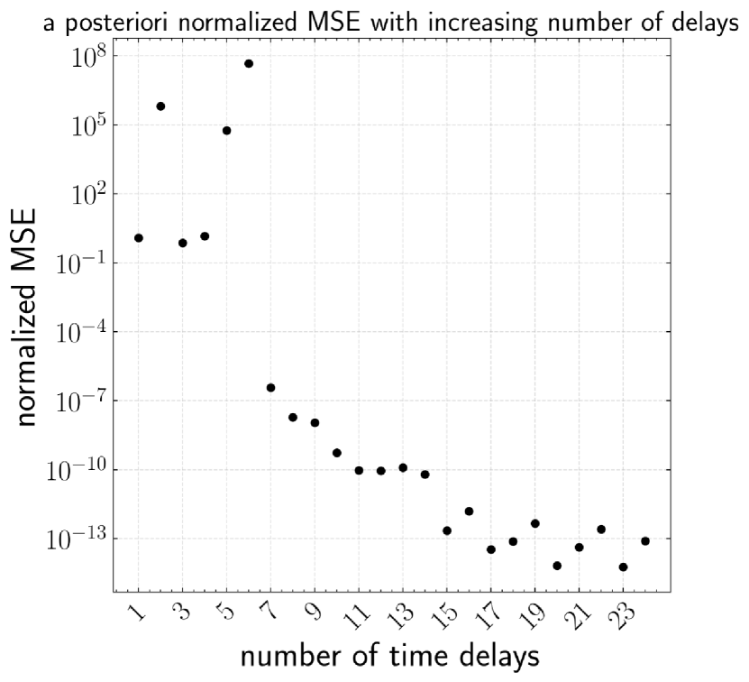
Figure 13: Top: Prediction vs ground truth for the toy quasi-periodic signal. Bottom: A posteriori MSE normalized by standard deviation with as a function of the number of time delays.

As shown in Figure 13, the linear model with $L=7$ accurately predicts the future state behavior of the quasi-periodic system with only a fraction of data limited in the range $[-0.25,0.55]$ while the whole data ranges from $[-0.944,0.902]$. Indeed, the minimal time delay $L=7$ is determined by the number of frequencies in the signal. The analysis on the minimal number of time delays for scalar time series as in Section III can be extended to quasi-periodic system. Consider the trigonometric identity, we have the following equivalent equation of Equation 79,

$$x(t)= \frac{1}{4}\bigg{(}\sin\Big{(}\frac{(\sqrt{2}+\sqrt{3}+2)t}{2}\Big{)}+\sin\Big{(}\frac{(\sqrt{2}+\sqrt{3}-2)t}{2}\Big{)}$$

$$-\sin\Big{(}\frac{(\sqrt{2}-\sqrt{3}+2)t}{2}\Big{)}-\sin\Big{(}\frac{(\sqrt{2}-\sqrt{3}-2)t}{2}\Big{)}\bigg{)}.$$

Therefore, we require $L=P-1=7$ time delays to fully recover the signal which is confirmed in Figure 13.

VII.3 Analysis of noise effect with pseudospectra

Note that our analysis and experiments thus far have been based on noise-free assumptions. When additive noise is present in the data, the minimal number of time delays as given by the results in Section III can be optimistic as we will confirm shortly. Alternatively, one might de-noise the data as by using for instance, optimal SVD thresholding Gavish and Donoho (2014) for the delay matrix with i.i.d. Gaussian noise. To illustrate the effect of noise, the toy 5-mode sine signal in Section VII.1.1 is considered, but the training horizon is increased to one complete period of data. Consider additive i.i.d. Gaussian noise with signal-to-noise ratio (with respect to the standard deviation) of 1%. To assess the influence of noise rigorously, we take an ensemble of 500 data trajectories and train a linear model with ordinary least squares on such data. In other words, for each sample trajectory, we have a slightly perturbed linear model associated with the data. The influence of noise is evaluated in the resulting distribution of eigenvalues (a priori sense) and long-time predictions (a posteriori sense). As shown in Figures 14 and 15, the theoretical optimality of $L=9$ does not hold as the model becomes overly dissipative. Instead, $L=20$ is required to have a reasonable prediction. It should be noted that the noise in the training data is too small to be observed in Figure 15, while the impact on the linear model is significant, as represented from the red shaded region. Moreover, as $L$ increases, it is observed that the “cloud" of eigenvalues shifts from the left half plane towards the imaginary. Interestingly, the “clouds" associated with spurious modes are much more scattered than those of the exact modes on the imaginary axis, i.e., the spurious modes are more sensitive to the noise in the data. As $L$ becomes increasingly large, e.g., $L=39$, those clouds merge together along the imaginary axis, resulting in higher uncertainty due to the possibility of unstable modes. This is also reflected in the a posteriori predictions in Figure 15. Interestingly, the ensemble average of a posteriori prediction appears to show better predictions, even though each individual prediction can be divergent. This implies that an appropriate Bayesian reformulation could make the model more robust to noise Pan and Duraisamy (2020).

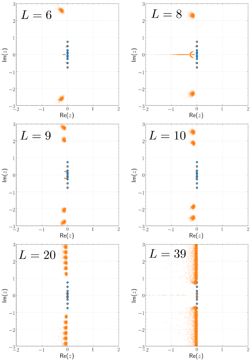
Figure 14: Eigenvalue distribution of linear model from noisy data with signal-to-noise ratio as 0.01 (orange) and noise-free data (blue). Time delay ranges from $L=6$ to $L=39$.

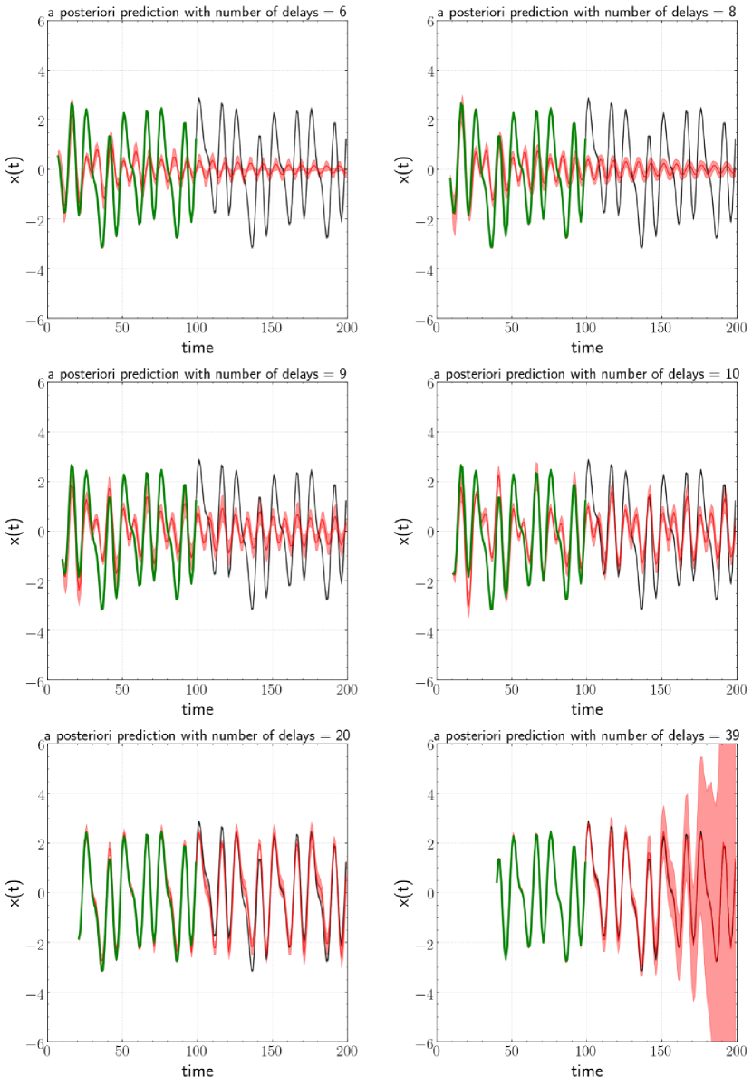
Figure 15: A posteriori prediction from noisy data with signal-to-noise ratio of 0.01. Green: training data. Black: whole data. Red: prediction from linear model. Shaded regions represents the uncertainty range of $\pm 2$ standard deviations. Note that all of training, whole and predictions contain shaded region but the noise on training/whole data is too small to be observed.

Next, we will analyze the robustness of the linear time delayed model with respect to noise in a more general sense. Recall that the previous analysis on condition number in Section VI.2.4 with periodic assumptions indicates robustness to noise with increasing time delays. For a more stringent description of the robustness, we introduce the concept of pseudospectra Trefethen et al. (1993). Here we define the $\epsilon$-pseudospectra of the block companion matrix $\mathbf{A}_{L}$ in Section VI.1 as $\Lambda_{\epsilon}$ in Equation 80.

$$\Lambda_{\epsilon}(\mathbf{A}_{L})=\{z\in\mathbb{C}:\sigma_{\textrm{min}}(z\mathbf{I}-\mathbf{A}_{L})\leq\epsilon\},$$ (80)

where $\sigma_{\textrm{min}}$ represents the minimal singular value. As shown in Figure 16, it is observed that the robustness of the solution decreases the increasing $L$ and becomes most sensitive to noise at the noise-free optimal $L=9$, following which the robustness improves as $L$ increases, which is consistent with previous analysis on condition number.

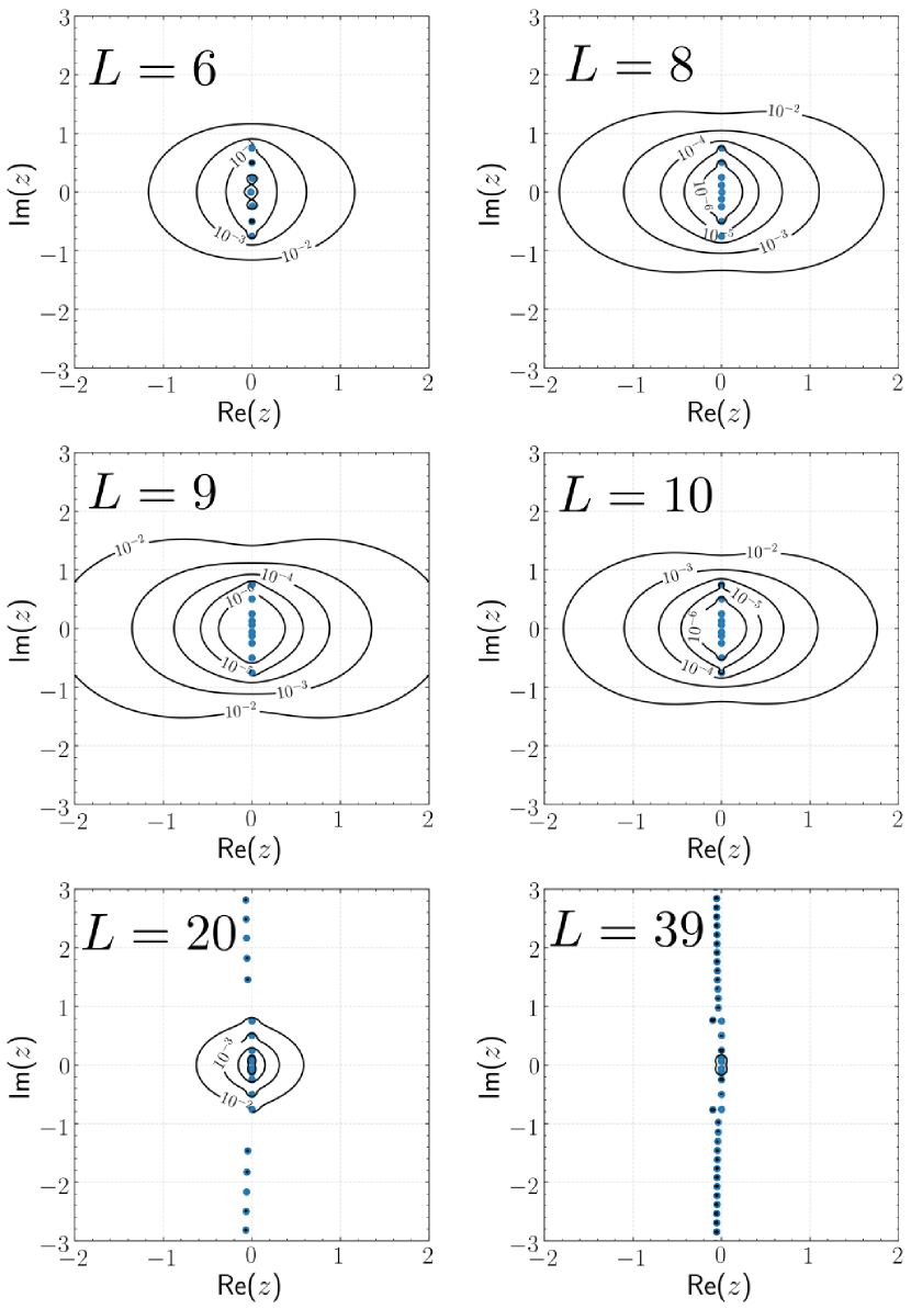
Figure 16: Isocontours of pseudospectra at $\epsilon=10^{-2}$, $10^{-3}$, $10^{-4}$, $10^{-5}$, $10^{-6}$ for different time delays $L$ for the toy 5 waves case.

VII.4 Turbulent Rayleigh-Bénard convection

As a final test case, we consider Rayleigh-Bénard convection, which is a problem of great interest to the fluid dynamics community. As displayed in Figure 17, the fluid is confined between two infinite horizontal planes with a hotter lower plane. The Rayleigh number, which represents the strength of buoyancy with respect to momentum and heat diffusion is defined as $Ra={U_{f}^{2}H^{2}}/{\nu\kappa}={\alpha g\Delta TH^{3}}/{\nu\kappa}$ where $\alpha$ is the thermal expansion coefficient, $\kappa$ is the thermal diffusivity, $\Delta T$ is the temperature difference between hot and cold planes, and $U_{f}\triangleq\sqrt{\alpha g\Delta TH}$ is the so-called free-fall velocity of a fluid parcel. Additional parameters that govern the dynamics are aspect ratio $\Gamma\triangleq L/H$, the Prandtl number $Pr=\nu/\kappa$. $L$ is the horizontal length scale of the domain. The computational domain is taken as a rectangular box with periodic side walls. We set $Ra=10^{7}$ for fully turbulence; $H=\pi L_{x}=\pi L_{y}$ and $Pr=1$. This domain is discretized uniformly in $x$ and $y$ direction with $128\times 128$ grid points and in $z$ direction with 128 grid points highly refined near the wall. The thickness of thermal boundary layer is sufficiently resolved Verzicco and Camussi (2003) since $\delta_{\theta}/H\sim{1}/{2Nu}\approx 10\Delta z$, where $\Delta z$ is the grid size in $z$ direction closest to the wall.

The simulation is performed by solving 3D incompressible Navier-Stokes equations with a Boussinesq approximation using OpenFOAM Jasak et al. (2007). Linear heat conduction, i.e., an unstable equilibrium state is set as initial condition. The simulation is performed over four thousand characteristic advection time units, approximately $1.264\tau_{\textrm{diff}}$, where $\tau_{\textrm{diff}}\triangleq{H^{2}}/{\nu}$, $\tau_{\textrm{adv}}\triangleq\sqrt{{H}/{\alpha g\Delta T}}$. The sampling interval is $\Delta t=4\tau_{\textrm{adv}}$. Note that this dynamical system contains approximately 2 million degrees of freedom. Here we perform dimension reduction on the sampled system state $u,v,w,T$ similar to Pan, Arnold-Medabalimi, and Duraisamy (2020). First, normalization for each component and mean subtraction is performed. Second, as shown in the bottom subfigure in the Figure 17, more than 99% of variance for the nonlinear system is retained in the first $r=800$ POD modes on the normalized data. After removing the effect of initial condition (the first 100 snapshots), we use 900 snapshots Pan and Arnold-Medabalimi (2020) for analysis.

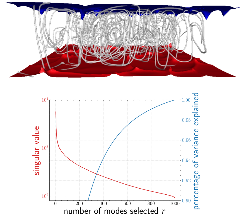
Figure 17: Top: Iso-surfaces of temperature at $T=295$ (red) and $T=285$ (blue) with streamlines of velocity field (grey) at $t=7.28$ for the Rayleigh-Bénard turbulent convection at $Ra=10^{7}$. Bottom: Singular value distribution and percentage of variance explained.

We consider the first 800 out of 900 snapshots as training data. Then we perform a posteriori evaluation for 900 steps to examine the reconstruction performance and predictions on future time steps. As shown in Figure 18, performing SVD-DMD ($L=0$) on this dataset with $r=800$ results in a set of unstable eigenvalues, leading to undesired blow up in a posteriori evaluation after $180\Delta t$. While the model with time delay $L=1$, overfits to the training data from $0$ to approximately $800\Delta t$, it yields stable predictions. Note that in this case $L_{opt}=\lceil{\frac{M}{r+1}}\rceil=1$.

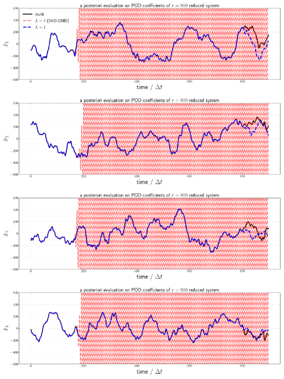
Figure 18: Comparison of a posteriori evaluation between linear model without/with time delay $L=1$ for the reduced system with $r=800$. Note that $0\leq t\leq 800$ is training horizon while $800<t\leq 900$ is testing horizon.

We then take the entire 900 snapshots trajectory as training data to investigate the impact of of time delays $L$ on stabilizing the reconstruction at various $r$. As shown in Figure 19, we first observe that as $r$ decreases, the numerical condition number increases simply as a consequence of retaining more small singular values. Secondly, we observe a general trend that, for each $r$, model performance worsens as $L$ increases from $0$ to $L_{opt}-1$, i.e., the transient point where linear systems approximately change from over-determined to under-determined. For the current data specifically, we observe that the system becomes stable as $L$ increases as the system becomes under-determined. Thirdly, we observe that the condition number shares a similar pattern with the reconstruction performance for each $r$.

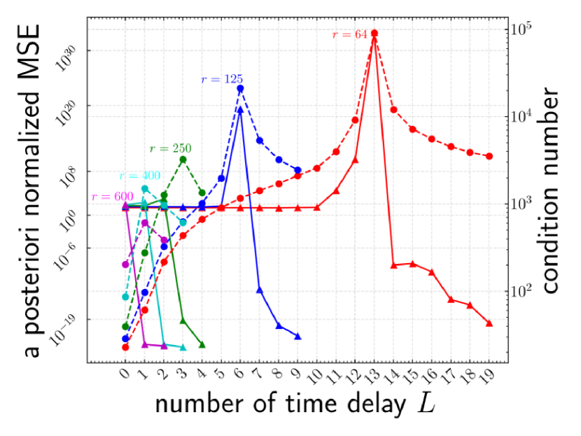
Figure 19: Dependency of model reconstruction performance and condition number on the number of time delays $L$ with varying reduced dimension $r$ for turbulent Rayleigh-Bénard convection. Solid line: normalized mean-squared-error. Dashed line: condition number.

VIII Conclusions

In summary, this work addressed fundamental questions regarding the structure and conditioning of linear time delay models of non-linear dynamics on an attractor. The following are the main contributions of this work:

1. We proved that for non-linear scalar dynamical systems, the number of time delays required by linear models to perfectly recover limit cycles is determined by the sparsity in the Fourier spectrum.

2. In the vector case, we proved that the minimal number of time delays has a tight upper bound that is precisely the output controllability index of a related linear system.

3. We developed an equivalent representation of the linear time delayed model in the spectral domain and provided the exact solution of the delay transition matrix $\mathbf{K}$ for the scalar case.

4. We derived an upper bound on the 2-norm condition number as a function of the sampling rate and the number of time delays. Thus, ill-conditioning can be mitigated by increasing the number of time delays and/or subsampling the original signal.

5. We explicitly showed that the dynamics over the full period can be perfectly recovered by training the linear time delayed model over just a partial period.

6. Influences of the noises are evaluated with ensemble realizations. We further analyzed the stability of the model with the concept of pseudospectra. The results are consistent with our finding on the stabilizing role of the number of time delays.

7. Numerical experiments on simple problems were shown to confirm each of the above theoretical results.

8. The impact of time delays on linear modeling of large-scale chaotic systems was investigated, and Hankel DMD was confirmed to produce stable and accurate results given enough time delays.

A few observations are pertinent to the above conclusions:

• Due to accuracy considerations on the numerical integrator, the sampling rate in the raw data may be excessively high. We believe that instabilities in prediction arise from choices that lead to poor numerical conditioning. Thus, as an alternate to pursuing explicit stabilization techniques Le Clainche and Vega (2017a); Champion, Brunton, and Kutz (2019), appropriate sub-sampling and time delays can be employed. Indeed, when noise is present in the data, explicit stabilization, Bayesian inference, or denoising techniques Rudy, Kutz, and Brunton (2019) may be warranted.

• The effectiveness of linear time delayed models of non-linear dynamics is that - by leveraging Fourier interpolation - an arbitrarily close trajectory from a high dimensional linear system can be derived. This also intuitively explains the ability of the model - when the signal has a sparse spectrum - to perform “true” predictions without training on a full period of data.

Data availability

The data that support the findings of this study are openly available in https://github.com/pswpswpsw/2020_Time_Delay_Paper_Rayleigh-Benard

Appendix A Proofs

A.1 Proof of Theorem 1

Proof.

Consider the discrete Fourier spectrum of $S_{M}(t)$ with $M$ uniform samples per period. The perfect prediction using a time-delayed linear model requires the existence of a real $\mathbf{K}$ that satisfies Equation 20, which is equivalent to Equation 26. Therefore, Equation 20 and Equation 26 share the same solutions in $\mathbb{C}^{(L+1)\times 1}$. Since the Fourier spectrum contains only $P$ non-zero coefficients, Equation 26 is equivalent to Equation 28. The necessary and sufficient condition to have a solution (not necessarily real) $\mathbf{K}$ for Equation 28 follows from the Rouché-Capelli theorem Meyer (2000),

$$\textrm{rank}\left(\begin{bmatrix}\mathbf{A}_{\mathcal{I}^{P}_{M},L}&\mathbf{b}_{\mathcal{I}^{P}_{M}}\end{bmatrix}\right)=\textrm{rank}\left(\mathbf{A}_{\mathcal{I}^{P}_{M},L}\right).$$ (81)

Using the first property in Lemma 1, rank$(\mathbf{A}_{\mathcal{I}_{M}^{P},L})=\min(P,L+1)$. While for the augmented matrix,

$$\textrm{rank}\left(\begin{bmatrix}\mathbf{A}_{\mathcal{I}^{P}_{M},L}&\mathbf{b}_{\mathcal{I}^{P}_{M}}\end{bmatrix}\right)=\textrm{rank}\left(\begin{bmatrix}\mathbf{b}_{\mathcal{I}^{P}_{M}}&\mathbf{A}_{\mathcal{I}^{P}_{M},L}\end{bmatrix}\right)$$ (82)

$$=\textrm{rank}\left(\begin{bmatrix}\omega^{i_{0}}&1&\omega^{-i_{0}}&\ldots&\omega^{-Li_{0}}\\ \omega^{i_{1}}&1&\omega^{-i_{1}}&\ldots&\omega^{-Li_{1}}\\ \vdots&\vdots&\vdots&\ddots&\vdots\\ \omega^{i_{P-1}}&1&\omega^{-i_{P-1}}&\ldots&\omega^{-Li_{P-1}}\end{bmatrix}\right)$$

$$=\textrm{rank}\left(\begin{bmatrix}\omega^{i_{0}}&&&&\\ &\omega^{i_{1}}&&&\\ &&&\ddots&\\ &&&&\omega^{i_{P-1}}\end{bmatrix}\begin{bmatrix}1&\omega^{-i_{0}}&\ldots&\omega^{-(L+1)i_{0}}\\ 1&\omega^{-i_{1}}&\ldots&\omega^{-(L+1)i_{1}}\\ \vdots&\vdots&\ddots&\vdots\\ 1&\omega^{-i_{P-1}}&\ldots&\omega^{-(L+1)i_{P-1}}\end{bmatrix}\right)$$

$$=\textrm{rank}\left(\operatorname{diag}(\omega^{i_{0}},\ldots,\omega^{i_{P-1}})\mathbf{V}_{L+2}(\omega^{-i_{0}},\ldots,\omega^{-i_{P-1}})\right)$$

$$=\textrm{rank}\left(\mathbf{V}_{L+2}(\omega^{-i_{0}},\ldots,\omega^{-i_{P-1}})\right)$$

$$=\min(P,L+2).$$

Therefore, if $L+2\leq P$, i.e., $L\leq P-2$, $\min(P,L+2)=L+2\neq L+1=\min(P,L+1)$. If $L+1\geq P$, i.e., $L\geq P-1$, then $\min(P,L+2)=P=\min(P,L+1)$. So the minimal $L$ for Equation 81 to hold is $P-1$, which makes $\mathbf{A}_{\mathcal{I}_{M}^{P},L}$ an invertible Vandermonde square matrix. Thus the solution is unique in $\mathbb{C}^{(L+1)\times 1}$. From Lemma 2, consider Equation 20, the solution is real. ∎

A.2 Proof of Theorem 2

Proof.

Consider

$$\mathcal{OC}(\mathbf{A,B,C};\mu)=\mathbf{C}\begin{bmatrix}\mathbf{B}&\mathbf{AB}&\ldots&\mathbf{A}^{\mu-1}\mathbf{B}\end{bmatrix}$$ (83)

$$=\mathbf{C}\begin{bmatrix}\mathbf{I}&\mathbf{A}&\ldots&\mathbf{A}^{\mu-1}\end{bmatrix}\begin{bmatrix}\mathbf{B}&&\\ &\ddots&\\ &&\mathbf{B}\end{bmatrix}$$

$$=\mathbf{EC}^{\prime}\begin{bmatrix}\mathbf{I}&&&&\mathbf{\Lambda}^{-(\mu-1)}&&\\ &\ddots&&\ldots&&\ddots&\\ &&\mathbf{I}&&&&\mathbf{\Lambda}^{-(\mu-1)}\end{bmatrix}\begin{bmatrix}\mathbf{e}&&\\ &\ddots&\\ &&\mathbf{e}\end{bmatrix}$$

$$=\mathbf{E}\begin{bmatrix}\operatorname{diag}(\mathbf{{a}}^{(1)})\mathbf{e}&\ldots&\operatorname{diag}(\mathbf{{a}}^{(J)})\mathbf{e}&\ldots&\operatorname{diag}(\mathbf{{a}}^{(1)})\mathbf{\Lambda}^{-(\mu-1)}\mathbf{e}&\ldots&\operatorname{diag}(\mathbf{{a}}^{(J)})\mathbf{\Lambda}^{-(\mu-1)}\mathbf{e}\end{bmatrix}.$$

Following Definition 3, for any integer $i\geq\mu$, $\mathcal{OC}(\mathbf{A,B,C};i)$ is full rank. Thus, $\forall v\in\mathbb{C}^{P\times 1}$, $v$ lies in the column space of $\mathcal{OC}(\mathbf{A,B,C};i)$. Therefore, $\mathbf{F}v$ should lie in the column space of $\mathbf{F}\mathcal{OC}(\mathbf{A,B,C};i)$. Noticing Lemma 4 and Remark 1, we have

$$\mathbf{F}v\in\textrm{Col}(\mathbf{F}\mathcal{OC}(\mathbf{A,B,C};i))=\mathcal{W}_{i-1}.$$ (84)

Now, consider $\forall j=1,\ldots,J$, $v^{(j)}=\mathbf{E}\operatorname{diag}(\mathbf{a}^{(j)})\mathbf{b}_{\mathcal{I}_{M}^{M}}\in\mathcal{C}^{P\times 1}$, from the above, we have

$$\mathbf{F}v^{(j)}=\mathbf{FE}\operatorname{diag}(\mathbf{a}^{(j)})\mathbf{b}_{\mathcal{I}_{M}^{M}}=\operatorname{diag}(\mathbf{a}^{(j)})\mathbf{b}_{\mathcal{I}_{M}^{M}}=\mathbf{c}^{(j)}\in\mathcal{W}_{i-1}.$$ (85)

Since the minimal $i$ for $\mathcal{OC}(\mathbf{A,B,C};i)$ to be full rank is $\mu$, the output observability index is $\mu$. Correspondingly, when the number of time delays $L=\mu-1$, a solution exists for Lemma 3, which makes $\mu-1$ an upper bound for the minimal time delay in Lemma 3. Finally, to show that the bounds are tight, consider that when $J=1$, Theorem 2 reverts to Theorem 1 where $\mu=P$, and thus $\mu-1=P-1$ is essentially the minimal number of time delays required. ∎

A.3 Proof of Lemma 1

Proof.

$$\mathbf{A}=\mathbf{V}_{N}(\alpha_{0},\alpha_{1},\ldots,\alpha_{M-1})=\begin{bmatrix}1&\alpha_{0}&\ldots&\alpha_{0}^{N-1}\\ 1&\alpha_{1}&\ldots&\alpha_{1}^{N-1}\\ \vdots&\vdots&\ddots&\vdots\\ 1&\alpha_{M-1}&\ldots&\alpha_{M-1}^{N-1}\end{bmatrix}$$ (86)

If $M\geq N$, then

$$\mathbf{V}_{N}(\alpha_{0},\alpha_{1},\ldots,\alpha_{M-1})=\begin{bmatrix}\mathbf{V}_{N}(\alpha_{0},\alpha_{1},\ldots,\alpha_{N-1})\\ \mathbf{V}_{N}(\alpha_{N},\ldots,\alpha_{M-1})\end{bmatrix}$$ (87)

Since $\{\alpha_{i}\}_{i\in\mathcal{I}_{M}}$ are distinct, $\mathbf{V}_{N}(\alpha_{0},\alpha_{1},\ldots,\alpha_{N-1})$ is full rank with rank $N$. Since $M\geq N$, the row space of $\mathbf{V}_{N}(\alpha_{0},\alpha_{1},\ldots,\alpha_{M-1})$ and is fully spanned by the first $N$ rows, and is thus full rank. Likewise, if $M<N$,

$$\mathbf{V}_{N}(\alpha_{0},\alpha_{1},\ldots,\alpha_{M-1})=\begin{bmatrix}\mathbf{V}_{M}(\alpha_{0},\alpha_{1},\ldots,\alpha_{M-1})&*\quad\end{bmatrix}$$ (88)

Similarly, the first $M$ columns are full rank and $\mathbf{V}_{N}(\alpha_{0},\alpha_{1},\ldots,\alpha_{M-1})$ is also full rank. Thus in either case, $\mathbf{V}_{N}(\alpha_{0},\alpha_{1},\ldots,\alpha_{M-1})$ is full rank with rank as $\min(M,N)$. To show the the second property, one can simply replace $\{\alpha_{i}\}_{i\in\mathcal{I}_{M}}$ with $\{\alpha_{i}\}_{i\in\mathcal{J}}$ in the above arguments. Since $|\mathcal{J}|=Q$, $\operatorname{rank}\left(\mathbf{V}_{N}(\{\alpha_{i}\}_{i\in\mathcal{J}})\right)=\min(Q,N)$. ∎

A.4 Proof of Lemma 2

Proof.

First, let’s prove from left to right. If $\exists\mathbf{x}\in\mathbb{C}^{n\times 1}$, we have $\mathbf{Ax}=\mathbf{b}$. Note that $\widebar{\mathbf{Ax}}=\widebar{\mathbf{A}}\widebar{\mathbf{x}}=\mathbf{A}\widebar{\mathbf{x}}=\widebar{\mathbf{b}}=\mathbf{b}$ then consider $\mathbf{x}^{\prime}=\frac{{\widebar{\mathbf{x}}+\mathbf{x}}}{2}\in\mathbb{R}^{n\times 1}$. $\mathbf{Ax^{\prime}}=(\mathbf{A}\mathbf{x}+\mathbf{A}\widebar{\mathbf{x}})/2=(\mathbf{b}+\mathbf{b})/2=\mathbf{b}$. Second, it is easy to show from right to left. Third, when uniqueness is added, note that $\mathbf{Ax=b}\iff\mathbf{A}\widebar{\mathbf{x}}=\mathbf{b}$, it is easy to show both directions since it is impossible to have complex solution being unique and not real. ∎

A.5 Proof of Lemma 3

Proof.

Given the definitions in Equations 44, 45 and 46, note Equation 16, we have

$$\mathbf{\tilde{Y}}_{k}=\begin{bmatrix}\mathbf{\Omega}_{k,L}&&\\ &\ddots&\\ &&\mathbf{\Omega}_{k,L}\end{bmatrix}\begin{bmatrix}\mathbf{a}^{(1)}\\ \vdots\\ \mathbf{a}^{(J)}\end{bmatrix}.$$ (89)

Recall Equation 19, note that

$$\mathbf{\Upsilon}_{k}=\mathbf{\Lambda}^{k}\mathbf{b}_{\mathcal{I}_{M}^{M}},$$ (90)

where $\mathbf{\Lambda}\triangleq\begin{bmatrix}1&&&\\ &\omega&&\\ &&\ddots&\\ &&&\omega^{(M-1)}\end{bmatrix}$.

Moreover, note that

$$\mathbf{\Omega}^{\top}_{k,L}=\mathbf{\Lambda}^{k}\mathbf{A}_{\mathcal{I}^{M}_{M},L}.$$ (91)

We rewrite Equation 45 for a given $k$ using Equation 18 for the left hand side and Equation 89 for the right hand side in Equation 45,

$$\begin{bmatrix}\mathbf{\Upsilon}_{k}^{\top}&&\\ &\ddots&\\ &&\mathbf{\Upsilon}_{k}^{\top}\end{bmatrix}\begin{bmatrix}\mathbf{a}^{(1)}\\ \vdots\\ \mathbf{a}^{(J)}\end{bmatrix}=\mathbf{\tilde{K}}^{\top}\begin{bmatrix}\mathbf{\Omega}_{k,L}&&\\ &\ddots&\\ &&\mathbf{\Omega}_{k,L}\end{bmatrix}\begin{bmatrix}\mathbf{a}^{(1)}\\ \vdots\\ \mathbf{a}^{(J)}\end{bmatrix}.$$ (92)

Using Equations 90 and 91 for the above, we have

$$\begin{bmatrix}\mathbf{a}^{(1)}\\ \vdots\\ \mathbf{a}^{(J)}\end{bmatrix}^{\top}\left(\begin{bmatrix}\mathbf{\Upsilon}_{k}&&\\ &\ddots&\\ &&\mathbf{\Upsilon}_{k}\end{bmatrix}\right)-\begin{bmatrix}\mathbf{\Omega}_{k,L}^{\top}&&\\ &\ddots&\\ &&\mathbf{\Omega}_{k,L}^{\top}\end{bmatrix}\mathbf{\tilde{K}}=\mathbf{0},$$ (93)

$$\begin{bmatrix}\mathbf{a}^{(1)}\\ \vdots\\ \mathbf{a}^{(J)}\end{bmatrix}^{\top}\begin{bmatrix}\mathbf{\Lambda}^{k}&&\\ &\ddots&\\ &&\mathbf{\Lambda}^{k}\end{bmatrix} \Bigg{(}\begin{bmatrix}\mathbf{b}_{\mathcal{I}^{M}_{M}}&&\\ &\ddots&\\ &&\mathbf{b}_{\mathcal{I}^{M}_{M}}\end{bmatrix}$$

$$-\begin{bmatrix}\mathbf{A}_{\mathcal{I}^{M}_{M},L}&&\\ &\ddots&\\ &&\mathbf{A}_{\mathcal{I}^{M}_{M},L}\end{bmatrix}\mathbf{\tilde{K}}\Bigg{)}=\mathbf{0}.$$ (94)

Considering $k=0,1,\ldots,M-1$, we stack $\begin{bmatrix}\mathbf{a}^{(1)}\\ \vdots\\ \mathbf{a}^{(J)}\end{bmatrix}^{\top}\begin{bmatrix}\mathbf{\Lambda}^{k}&&\\ &\ddots&\\ &&\mathbf{\Lambda}^{k}\end{bmatrix}$ row by row as

$$\begin{bmatrix}a_{0}^{(1)}&\ldots&a_{M-1}^{(1)}&\ldots&a_{0}^{(J)}&\ldots&a_{M-1}^{(J)}\\ a_{0}^{(1)}&\ldots&\omega^{M-1}a_{M-1}^{(1)}&\ldots&a_{0}^{(J)}&\ldots&\omega^{M-1}a_{M-1}^{(J)}\\ \vdots&\ddots&\vdots&\ldots&\vdots&\ddots&\vdots\\ a_{0}^{(1)}&\ldots&\omega^{(M-1)^{2}}a_{M-1}^{(1)}&\ldots&a_{0}^{(J)}&\ldots&\omega^{(M-1)^{2}}a_{M-1}^{(J)}\end{bmatrix}$$

$$=\mathbf{V}_{M}(\{\omega^{j}\}_{j=0}^{M-1})\begin{bmatrix}\mathbf{I}&\ldots&\mathbf{I}\end{bmatrix}\operatorname{diag}(\{\mathbf{a}^{(l)}\}_{l=1}^{J})$$

$$=\mathbf{V}_{M}(\{\omega^{j}\}_{j=0}^{M-1})\begin{bmatrix}\operatorname{diag}(\mathbf{a}^{(1)})&\ldots&\operatorname{diag}(\mathbf{a}^{(J)})\end{bmatrix}.$$ (95)

Then plug the above equality into Equation 94, and notice the non-singularity of $\mathbf{V}_{M}(\{\omega^{j}\}_{j=0}^{M-1})$, for $k=0,1,\ldots,M-1$, Equation 94 can be rewritten as

$$\begin{bmatrix}\operatorname{diag}(\mathbf{a}^{(1)})&\ldots&\operatorname{diag}(\mathbf{a}^{(J)})\end{bmatrix}\Bigg{(}\begin{bmatrix}\mathbf{b}_{\mathcal{I}^{M}_{M}}&&\\ &\ddots&\\ &&\mathbf{b}_{\mathcal{I}^{M}_{M}}\end{bmatrix}$$

$$-\begin{bmatrix}\mathbf{A}_{\mathcal{I}^{M}_{M},L}&&\\ &\ddots&\\ &&\mathbf{A}_{\mathcal{I}^{M}_{M},L}\end{bmatrix}\mathbf{\tilde{K}}\Bigg{)}=\mathbf{0}.$$ (96)

From the Rouché-Capelli theorem Meyer (2000), the necessary and sufficient condition for the existence of a complex solution to Equation 96 is,

$$\operatorname{rank}\Big{(} \begin{bmatrix}\operatorname{diag}(\mathbf{a}^{(1)})\mathbf{A}_{\mathcal{I}^{M}_{M},L}&\ldots&\operatorname{diag}(\mathbf{a}^{(J)})\mathbf{A}_{\mathcal{I}^{M}_{M},L}\end{bmatrix}\Bigg{)}$$

$$=\operatorname{rank}\Big{(}\Big{[} \operatorname{diag}(\mathbf{a}^{(1)})\mathbf{A}_{\mathcal{I}^{M}_{M},L}\ldots\operatorname{diag}(\mathbf{a}^{(J)})\mathbf{A}_{\mathcal{I}^{M}_{M},L}$$ (97)

$$\operatorname{diag}(\mathbf{a}^{(1)})\mathbf{b}_{\mathcal{I}^{M}_{M}}\ldots\operatorname{diag}(\mathbf{a}^{(J)})\mathbf{b}_{\mathcal{I}^{M}_{M}}\Big{]}\Big{)}.$$ (98)

Note that since the above procedures are can be retained in Equation 45, Equation 45 and Equation 96 share the same solution in $\mathbb{C}^{J(L+1)\times J}$. From Lemma 2, Equation 97 is also the necessary and sufficient condition for Equation 45 to have a real solution. ∎

A.6 Proof of Lemma 4

Proof.

For $n,J\in\mathbb{N}$, consider $J$ diagonal matrices in $\mathbf{A}$, for $j=1,\ldots,J$, with the $j$-th diagonal matrices being $\operatorname{diag}(\mathbf{a}^{(j)})\in\mathbb{C}^{n\times n}$. $\mathbf{a}^{(j)}=\begin{bmatrix}\mathbf{a}^{(j)}_{1}&\mathbf{a}^{(j)}_{2}&\ldots\mathbf{a}^{(j)}_{n}\end{bmatrix}^{\top}$. Thus

$$\mathbf{A}=\begin{bmatrix}\operatorname{diag}(\mathbf{a}^{(1)})&\operatorname{diag}(\mathbf{a}^{(2)})&\ldots&\operatorname{diag}(\mathbf{a}^{(J)})\end{bmatrix}\in\mathbb{C}^{n\times nJ}.$$

We define the following row index set that describes the row that is not a zero row vector in $\mathbf{A}$.

$$\Gamma=\{l|l\in\{1,\ldots,n\},\exists j\in\{1,\ldots,J\},\mathbf{a}^{(j)}_{l}\neq 0\},$$ (99)

where we further order the index in $\Gamma$ as

$$1\leq\gamma_{1}<\gamma_{2}<\ldots<\gamma_{P}\leq n,$$

where $P=|\Gamma|$. Now we construct the row elimination matrix $\mathbf{E}\in\mathbb{C}^{P\times n}$ from $\Gamma$ with

$$i\in\{1,\ldots,P\},j\in\{1,\ldots,n\},\mathbf{E}_{ij}=\delta_{\gamma_{i},j}.$$ (100)

For $\mathbf{EA}$, since $\mathbf{E}$ only removes the zero row vector, the rank of the matrix $\mathbf{EA}$ is the same as $\mathbf{A}$. To show $\mathbf{EA}$ is full rank, simply consider the following procedure:

From the definition of $\Gamma$, on each row with row index $i=1,\ldots,P$, there are non-zero entries. Start by choosing an entry, denoted as $\mathbf{a}_{\gamma_{i}}^{j_{i}}$ that is non-zero (while the choice of $j_{i}$ is not unique). Then, one can simply perform column operations that switch the column with index ${j_{i}}$ corresponding to the non-zero entry of $i$-th row, with the current $i$-th column. These operations can be iteratively performed, after which the following matrix is obtained:

$$\mathbf{EA}\mathbf{R}=\begin{bmatrix}\mathbf{a}_{\gamma_{1}}^{j_{1}}&&&&*&\\ &\mathbf{a}_{\gamma_{2}}^{j_{2}}&&&*&\\ &&\ddots&&*&\\ &&&\mathbf{a}_{\gamma_{P}}^{j_{P}}&*&\end{bmatrix},$$ (101)

where $\forall i=1,\ldots,P,\mathbf{a}_{\gamma_{i}}^{j_{i}}\neq 0$ and $\mathbf{R}$ is the elementary column operation matrix. Thus $\mathbf{EAR}$ is full rank, and $\mathbf{EA}$ is full rank.

Define $\mathbf{F}=\mathbf{E}^{\top}$, i.e., $\mathbf{F}_{jk}=\delta_{\gamma_{k},j}$. Thus

$$i,j\in\{1,\ldots,n\},\mathbf{G}_{ij}\triangleq\mathbf{F}_{ik}\mathbf{E}_{kj}=\delta_{\gamma_{k},i}\delta_{\gamma_{k},j}$$

$$=\sum_{k=1}^{P}\delta_{\gamma_{k},i}\delta_{\gamma_{k},j}=\begin{cases}1,\textrm{ $i=j\in\Gamma$, }\\ 0,\textrm{ otherwise. }\end{cases}$$ (102)

Therefore, $\mathbf{G}$ is simply a diagonal matrix that keeps the row with index in $\Gamma$ unchanged, but makes the row zero when the index is not in $\Gamma$. However, the row index that is not in $\Gamma$ corresponds to a zero row vector, and thus $\mathbf{GA}=\mathbf{A}$, i.e., $\mathbf{E}^{\top}\mathbf{EA}=\mathbf{A}.$ ∎

A.7 Proof of Lemma 5

Proof.

For $q\in\mathbb{N}$, denote $L_{q}=qM+P-1$. Note that in Equation 28, when $L=P-1$, the minimal 2-norm solution $\mathbf{\hat{K}}_{P-1}$ is also unique. Specifically we denote $\mathbf{\hat{K}}_{P-1}=\begin{bmatrix}\hat{K}_{0}&\ldots&\hat{K}_{P-1}\end{bmatrix}$. Note that, for any $L\geq P-1$, we can find $q=\left\lfloor{\frac{L-P+1}{M}}\right\rfloor$, such that $L\in\mathcal{T}_{q}\triangleq[L_{q},L_{q+1})$. From the definition of the minimal 2-norm solution, we have $\lVert\mathbf{\hat{K}}_{L}\rVert_{2}\leq\lVert\mathbf{\hat{K}}_{L_{q}}\rVert_{2}$.

Consider $\mathbf{A}_{\mathcal{I}^{P}_{M},L_{q}}$ and notice that for $q=0$, i.e., $L_{0}=P-1\leq L<L_{1}=M+P-1$, so $\lVert\mathbf{\hat{K}}_{L}\rVert_{2}\leq\lVert\mathbf{\hat{K}}_{L_{0}}\rVert_{2}=\lVert\mathbf{\hat{K}}_{P-1}\rVert_{2}$; for $q\geq 1$, for any $1\leq j\leq P$, the $j$-th column of $\mathbf{A}_{\mathcal{I}^{P}_{M},L_{q}}$ is duplicated with the $(j+kM)$-th column, $k=1,\ldots,q$. For $q\geq 1$, $\mathbf{A}_{\mathcal{I}^{P}_{M},L_{q}}$ in Equation 28, consider the following easily validated special class of real solutions,

$$\mathbf{K}=\begin{bmatrix}K_{0}\\ \vdots\\ K_{P-1}\\ 0\\ \vdots\\ 0\\ K_{M}\\ \vdots\\ K_{L_{1}}\\ 0\\ \vdots\\ 0\\ \vdots\\ K_{qM}\\ \vdots\\ K_{L_{q}}\end{bmatrix}^{\top}\in\mathbb{R}^{1\times(L_{q+1})},$$ (103)

with the constraint that for any $1\leq j\leq P$, $\sum_{l=0}^{q}K_{j-1+lM}={\hat{K}}_{j-1}$. To find the minimal 2-norm solution, note that we have

$$\min\lVert\mathbf{K}\rVert_{2}^{2}=\sum_{j=1}^{P}\min\sum_{l=0}^{q}K^{2}_{j-1+lM}.$$ (104)

From Jensen’s inequality, $\forall j=1,\ldots,P$,

$$\frac{\sum_{l=0}^{q}K^{2}_{j-1+lM}}{q+1} \geq\left(\frac{\sum_{l=0}^{q}K_{j-1+lM}}{q+1}\right)^{2},$$ (105)

$$\sum_{l=0}^{q}K^{2}_{j-1+lM} \geq\frac{\hat{K}_{j-1}^{2}}{q+1},$$ (106)

where the equality holds when $K_{j-1+lM}={\hat{K}_{j-1}}/{(q+1)}$ for $l=0,\ldots,q$. Thus $\min\lVert\mathbf{K}\rVert_{2}^{2}=\sum_{j=1}^{P}\hat{K}_{j-1}^{2}/(q+1)=\lVert\mathbf{\hat{K}}_{P-1}\rVert_{2}^{2}/(q+1)$. Since the above minimal norm is found within a special class of solutions in Equation 28, the general minimal 2-norm is

$$\lVert\mathbf{\hat{K}}_{L}\rVert_{2}^{2}\leq\lVert\mathbf{\hat{K}}_{L_{q}}\rVert_{2}^{2}\leq\lVert\mathbf{\hat{K}}_{P-1}\rVert_{2}^{2}/(q+1).$$

Combining both cases for $q=0$ and $q\geq 1$, we have the desired result. ∎

A.8 Proof of Proposition 3

Proof.

To begin with, consider the following under-determined linear system for $f\in\mathbb{R}^{N}$, given $N\geq n$

$$\mathbf{V}_{N}(z_{1},\ldots,z_{n})f=\operatorname{diag}(z_{1},\ldots,z_{n})\mathbf{e},$$ (107)

where $\mathbf{e}=\begin{bmatrix}1&1&\ldots&1\end{bmatrix}^{\top}$. Denote ${f}_{N}$ to be the minimum 2-norm solution. Suppose for all nodes, $i=1,\ldots,n$, $|z_{i}|\leq 1$. Bazán Bazán (2000) showed that

$$\lim_{N\rightarrow+\infty}\lVert f_{N}\rVert_{2}=0.$$ (108)

Consider multiplying Equation 28 on both sides from the left with $\operatorname{diag}(\omega^{Li_{0}},\ldots,\omega^{Li_{P-1}})$. Notice that the diagonal matrix is non-singular for any $L\in\mathbb{N}$, and the inverse of permutation matrix is its transpose. Then we have

$$\begin{bmatrix}\omega^{Li_{0}}&\omega^{(L-1)i_{0}}&\ldots&1\\ \vdots&\vdots&\vdots&\vdots\\ \omega^{Li_{P-1}}&\omega^{(L-1)i_{P-1}}&\ldots&1\\ \end{bmatrix}\mathbf{K}=\begin{bmatrix}\omega^{(L+1)i_{0}}\\ \vdots\\ \omega^{(L+1)i_{P-1}}\end{bmatrix},$$ (109)

$$\begin{bmatrix}1&\omega^{i_{0}}&\ldots&\omega^{Li_{0}}\\ \vdots&\vdots&\vdots&\vdots\\ 1&\omega^{i_{P-1}}&\ldots&\omega^{Li_{P-1}},\\ \end{bmatrix}\mathbf{P}^{\top}\mathbf{K}=\begin{bmatrix}\omega^{i_{0}}&&\\ &\ddots&\\ &&\omega^{i_{P-1}}\end{bmatrix}^{L+1}\mathbf{e},$$ (110)

$$\mathbf{V}_{L+1}(\omega^{i_{0}},\ldots,\omega^{i_{P-1}})f=(\operatorname{diag}(\omega^{i_{0}},\ldots,\omega^{i_{P-1}}))^{L+1}\mathbf{e},$$ (111)

where $f\triangleq\mathbf{P}^{\top}\mathbf{K}$, $\mathbf{P}\in\mathbb{R}^{(L+1)\times(L+1)}$ is the column permutation matrix that reverses the column order in $\mathbf{A}_{\mathcal{I}^{P}_{M},L}$. Note that a solution exists when $L+1=P$ and it is not unique when $L+1>P$. Denote $f_{L}$ as the corresponding minimal 2-norm solution of Equation 111. From Equation 108, consider Equation 111 and take $L\rightarrow+\infty$, $\lVert f_{L}\rVert_{2}\rightarrow 0$. The row permutation matrix does not change the 2-norm of a vector, and hence there is a one-to-one correspondence between the solution in Equation 111 and Equation 28, such that the corresponding minimal 2-norm solution for Equation 28 is $\mathbf{\hat{K}}_{L}\triangleq\mathbf{P}f_{L}$ thus $\lVert\mathbf{\hat{K}}_{L}\rVert_{2}\rightarrow 0$. ∎

A.9 Proof of Proposition 4

Proof.

Consider the fact that the Vandermonde matrix $\mathbf{V}_{N}(z_{1},\ldots,z_{n})$ with $n$ distinct nodes $\{z_{i}\}_{i=1}^{n}$, $z_{i}\in\mathbb{C}$ of order $N$, $N\geq n$, i.e., $\mathbf{V}_{N}$ is full rank. The Frobenius-norm condition number is defined as $\kappa_{F}(\mathbf{V}_{N})\triangleq\lVert\mathbf{V}_{N}\rVert_{F}\lVert\mathbf{V}_{N}^{\dagger}\rVert_{F}$, where $\dagger$ represents Moore-Penrose pseudoinverse. Bazán Bazán (2000) showed that if $\forall i=1,\ldots,n$, with distinct $|z_{i}|\leq 1$, $N\geq n$, then

$$\kappa_{F}(\mathbf{V}_{N})\leq n\left[1+\frac{(n-1)+\lVert f_{N}\rVert_{2}^{2}+\prod_{i=1}^{n}|z_{i}|^{2}-\sum_{i=1}^{n}|z_{i}|^{2}}{(n-1)\delta^{2}}\right]^{\frac{n-1}{2}}\phi_{N}(\alpha,\beta),$$ (112)

where $\displaystyle\delta\triangleq\min_{1\leq i<j\leq n}|z_{i}-z_{j}|$, $\phi_{N}(\alpha,\beta)\triangleq\sqrt{\frac{1+\alpha^{2}+\ldots+\alpha^{2(N-1)}}{1+\beta^{2}+\ldots+\beta^{2(N-1)}}}$, $\displaystyle\alpha\triangleq\max_{1\leq j\leq n}|z_{j}|$, $\displaystyle\beta\triangleq\min_{1\leq j\leq n}|z_{j}|$.

The key to understand the behavior of the upper bound of $\kappa_{2}(\mathbf{V}_{N})$, is to estimate the convergence rate of $\lVert f_{N}\rVert_{2}$ which is considered difficult for a general distribution of nodes Bazán (2000). For the particular case of Equation 28, we can show a tight upper bound in Lemma 5. Thus, $\forall 1\leq i\leq n,|z_{i}|=1$, Equation 112 becomes,

$$\kappa_{F}(\mathbf{V}_{N}) \leq n\left(1+\frac{\lVert f_{N}\rVert_{2}^{2}}{(n-1)\delta^{2}}\right)^{\frac{n-1}{2}}.$$ (113)

Now we note a general inequality between the condition number in the 2-norm and in the Frobenius norm Bazán (2000) by considering,

$$n-2<n-2+\kappa_{2}(\mathbf{V}_{N})+\kappa_{2}^{-1}(\mathbf{V}_{N})\leq\kappa_{F}(\mathbf{V}_{N}),$$ (114)

$$\kappa_{2}(\mathbf{V}_{N})\leq\frac{1}{2}\left[\kappa_{F}(\mathbf{V}_{N})-n+2+\sqrt{(\kappa_{F}(\mathbf{V}_{N})-n+2)^{2}-4}\right].$$ (115)

The right hand side in Equation 115 is monotonically increasing with respect to $\kappa_{F}(\mathbf{V}_{N})$. Therefore using the upper bound from Equation 113 in Equation 115, and some algebra we have the following upper bound, $\forall N>n$,

$$\kappa_{2}(\mathbf{V}_{N})\leq 1+\frac{d}{2}\left[1+\sqrt{1+\frac{4}{d}}\right],$$ (116)

where

$$d\triangleq n\left[\left(1+\frac{\lVert f_{N}\rVert_{2}^{2}}{(n-1)\delta^{2}}\right)^{\frac{n-1}{2}}-1\right].$$ (117)

Finally, note that $d$ monotonically increases with $\lVert f_{N}\rVert_{2}$, and thus with $n=P$, $N=L+1$, $z_{l}=\omega^{-i_{l}}$, $l=0,\ldots,P-1$ and Lemma 5, the desired upper bound is achieved. As $L\rightarrow\infty$, $\mathbf{\hat{K}}_{L}\rightarrow 0$ and $d\rightarrow 0$, and thus it is trivial to show that $\kappa_{2}(\mathbf{A}_{\mathcal{I}_{M}^{P},L})\rightarrow 1$. ∎

References

- Chen and Billings (1989) S. Chen and S. A. Billings, “Representations of non-linear systems: the NARMAX model,” International Journal of Control 49, 1013–1032 (1989).
- Hegger, Kantz, and Schreiber (1999) R. Hegger, H. Kantz, and T. Schreiber, “Practical implementation of nonlinear time series methods: The TISEAN package,” Chaos: An Interdisciplinary Journal of Nonlinear Science 9, 413–435 (1999).
- Arbabi and Mezic (2017) H. Arbabi and I. Mezic, “Ergodic theory, dynamic mode decomposition, and computation of spectral properties of the Koopman operator,” SIAM Journal on Applied Dynamical Systems 16, 2096–2126 (2017).
- Arbabi and Mezić (2017) H. Arbabi and I. Mezić, “Study of dynamics in post-transient flows using Koopman mode decomposition,” Physical Review Fluids 2, 124402 (2017).
- Kamb et al. (2018) M. Kamb, E. Kaiser, S. L. Brunton, and J. N. Kutz, “Time-delay observables for Koopman: Theory and applications,” arXiv preprint arXiv:1810.01479 (2018).
- Brunton et al. (2017) S. L. Brunton, B. W. Brunton, J. L. Proctor, E. Kaiser, and J. N. Kutz, “Chaos as an intermittently forced linear system,” Nature communications 8, 19 (2017).
- Pan and Duraisamy (2018a) S. Pan and K. Duraisamy, “Data-Driven Discovery of Closure Models,” SIAM Journal on Applied Dynamical Systems 17, 2381–2413 (2018a).
- Takens (1981) F. Takens, “Detecting strange attractors in turbulence,” in Dynamical systems and turbulence, Warwick 1980 (Springer, 1981) pp. 366–381.
- Sauer, Yorke, and Casdagli (1991) T. Sauer, J. A. Yorke, and M. Casdagli, “Embedology,” Journal of statistical Physics 65, 579–616 (1991).
- Stark et al. (2003a) J. Stark, D. S. Broomhead, M. E. Davies, and J. Huke, “Delay embeddings for forced systems. I. Deterministic forcing,” Journal of Nonlinear Science 13, 519–577 (2003a).
- Stark et al. (2003b) J. Stark, D. S. Broomhead, M. Davies, and J. Huke, “Delay embeddings for forced systems. II. stochastic forcing,” Journal of Nonlinear Science 13, 519–577 (2003b).
- Deyle and Sugihara (2011) E. R. Deyle and G. Sugihara, “Generalized theorems for nonlinear state space reconstruction,” PLoS One 6 (2011).
- Box et al. (2015) G. E. Box, G. M. Jenkins, G. C. Reinsel, and G. M. Ljung, Time series analysis: forecasting and control (John Wiley & Sons, 2015).
- Frank, Davey, and Hunt (2001) R. J. Frank, N. Davey, and S. P. Hunt, “Time series prediction and neural networks,” Journal of intelligent and robotic systems 31, 91–103 (2001).
- Lang, Waibel, and Hinton (1990) K. J. Lang, A. H. Waibel, and G. E. Hinton, “A time-delay neural network architecture for isolated word recognition,” Neural networks 3, 23–43 (1990).
- Peddinti, Povey, and Khudanpur (2015) V. Peddinti, D. Povey, and S. Khudanpur, “A time delay neural network architecture for efficient modeling of long temporal contexts,” in Sixteenth Annual Conference of the International Speech Communication Association (2015).
- Bromley et al. (1994) J. Bromley, I. Guyon, Y. LeCun, E. Säckinger, and R. Shah, “Signature verification using a “siamese" time delay neural network,” in Advances in neural information processing systems (1994) pp. 737–744.
- Goodfellow et al. (2016) I. Goodfellow, Y. Bengio, A. Courville, and Y. Bengio, Deep learning, Vol. 1 (MIT press Cambridge, 2016).
- Ma, Wang et al. (2018) C. Ma, J. Wang, et al., “Model reduction with memory and the machine learning of dynamical systems,” arXiv preprint arXiv:1808.04258 (2018).
- Le Clainche and Vega (2017a) S. Le Clainche and J. M. Vega, “Higher order dynamic mode decomposition,” SIAM Journal on Applied Dynamical Systems 16, 882–925 (2017a).
- Kaiser, Kutz, and Brunton (2018) E. Kaiser, J. N. Kutz, and S. L. Brunton, “Sparse identification of nonlinear dynamics for model predictive control in the low-data limit,” Proceedings of the Royal Society A 474, 20180335 (2018).
- Gilmore and Lefranc (2003) R. Gilmore and M. Lefranc, “The topology of chaos,” (2003).
- McGuinness (1983) M. J. McGuinness, “The fractal dimension of the lorenz attractor,” Physics Letters A 99, 5–9 (1983).
- Abarbanel et al. (1993) H. D. Abarbanel, R. Brown, J. J. Sidorowich, and L. S. Tsimring, “The analysis of observed chaotic data in physical systems,” Reviews of modern physics 65, 1331 (1993).
- Kennel, Brown, and Abarbanel (1992) M. B. Kennel, R. Brown, and H. D. Abarbanel, “Determining embedding dimension for phase-space reconstruction using a geometrical construction,” Physical review A 45, 3403 (1992).
- Broomhead and Jones (1989) D. S. Broomhead and R. Jones, “Time-series analysis,” Proc. R. Soc. Lond. A 423, 103–121 (1989).
- Sugihara, Grenfell, and May (1990) G. Sugihara, B. T. Grenfell, and R. M. May, “Distinguishing error from chaos in ecological time series,” Phil. Trans. R. Soc. Lond. B 330, 235–251 (1990).
- Sauer and Yorke (1993) T. Sauer and J. A. Yorke, “How many delay coordinates do you need?” International Journal of Bifurcation and Chaos 3, 737–744 (1993).
- Kim, Eykholt, and Salas (1999) H. Kim, R. Eykholt, and J. Salas, “Nonlinear dynamics, delay times, and embedding windows,” Physica D: Nonlinear Phenomena 127, 48–60 (1999).
- Cao (1997) L. Cao, “Practical method for determining the minimum embedding dimension of a scalar time series,” Physica D: Nonlinear Phenomena 110, 43–50 (1997).
- Liu, Ng, and Quek (2007) F. Liu, G. S. Ng, and C. Quek, “RLDDE: A novel reinforcement learning-based dimension and delay estimator for neural networks in time series prediction,” Neurocomputing 70, 1331–1341 (2007).
- Lomax and Hahs-Vaughn (2013) R. G. Lomax and D. L. Hahs-Vaughn, Statistical concepts: A second course (Routledge, 2013).
- Gouasmi, Parish, and Duraisamy (2017) A. Gouasmi, E. J. Parish, and K. Duraisamy, “A priori estimation of memory effects in reduced-order models of nonlinear systems using the mori–zwanzig formalism,” Proc. R. Soc. A 473, 20170385 (2017).
- Chorin and Hald (2014) A. J. Chorin and O. H. Hald, “Estimating the uncertainty in underresolved nonlinear dynamics,” Mathematics and Mechanics of Solids 19, 28–38 (2014).
- Parish, Wentland, and Duraisamy (2018) E. J. Parish, C. Wentland, and K. Duraisamy, “The Adjoint Petrov-Galerkin Method for Non-Linear Model Reduction,” arXiv e-prints (2018), arXiv:1810.03455 [math.DS] .
- Juang and Pappa (1985) J.-N. Juang and R. S. Pappa, “An eigensystem realization algorithm for modal parameter identification and model reduction,” Journal of guidance, control, and dynamics 8, 620–627 (1985).
- Vautard, Yiou, and Ghil (1992) R. Vautard, P. Yiou, and M. Ghil, “Singular-spectrum analysis: A toolkit for short, noisy chaotic signals,” Physica D: Nonlinear Phenomena 58, 95–126 (1992).
- Tu et al. (2014) J. H. Tu, C. W. Rowley, D. M. Luchtenburg, S. L. Brunton, and J. N. Kutz, “On dynamic mode decomposition: Theory and applications,” Journal of Computational Dynamics 1, 391–421 (2014).
- Champion, Brunton, and Kutz (2019) K. P. Champion, S. L. Brunton, and J. N. Kutz, “Discovery of nonlinear multiscale systems: Sampling strategies and embeddings,” SIAM Journal on Applied Dynamical Systems 18, 312–333 (2019).
- Broomhead and King (1986) D. S. Broomhead and G. P. King, “Extracting qualitative dynamics from experimental data,” Physica D: Nonlinear Phenomena 20, 217–236 (1986).
- Gibson et al. (1992) J. F. Gibson, J. Doyne Farmer, M. Casdagli, and S. Eubank, “An analytic approach to practical state space reconstruction,” Physica. D, Nonlinear phenomena 57, 1–30 (1992).
- Schmid (2010) P. J. Schmid, “Dynamic mode decomposition of numerical and experimental data,” Journal of fluid mechanics 656, 5–28 (2010).
- Brunton, Proctor, and Kutz (2013) S. L. Brunton, J. L. Proctor, and J. N. Kutz, “Compressive sampling and dynamic mode decomposition,” arXiv preprint arXiv:1312.5186 (2013).
- Pope (2000) S. B. Pope, Turbulent Flows (Cambridge University Press, 2000).
- Pan and Johnsen (2017) S. Pan and E. Johnsen, “The role of bulk viscosity on the decay of compressible, homogeneous, isotropic turbulence,” Journal of Fluid Mechanics 833, 717–744 (2017).
- Schilder et al. (2006) F. Schilder, W. Vogt, S. Schreiber, and H. M. Osinga, “Fourier methods for quasi-periodic oscillations,” International journal for numerical methods in engineering 67, 629–671 (2006).
- Rowley et al. (2009) C. W. Rowley, I. Mezić, S. Bagheri, P. Schlatter, and D. S. Henningson, “Spectral analysis of nonlinear flows,” Journal of fluid mechanics 641, 115–127 (2009).
- Mezić (2005) I. Mezić, “Spectral properties of dynamical systems, model reduction and decompositions,” Nonlinear Dynamics 41, 309–325 (2005).
- Willcox and Megretski (2005) K. Willcox and A. Megretski, “Fourier series for accurate, stable, reduced-order models in large-scale linear applications,” SIAM Journal on Scientific Computing 26, 944–962 (2005).
- Gugercin and Willcox (2008) S. Gugercin and K. Willcox, “Krylov projection framework for Fourier model reduction,” Automatica 44, 209–215 (2008).
- Lipton and Dabke (1996) J. Lipton and K. Dabke, “Reconstructing the state space of continuous time chaotic systems using power spectra,” Physics Letters A 210, 290–300 (1996).
- Kutz et al. (2016) J. N. Kutz, S. L. Brunton, B. W. Brunton, and J. L. Proctor, Dynamic mode decomposition: data-driven modeling of complex systems (SIAM, 2016).
- Le Clainche and Vega (2017b) S. Le Clainche and J. M. Vega, “Higher order dynamic mode decomposition to identify and extrapolate flow patterns,” Physics of Fluids 29, 084102 (2017b).
- Beltrán, Le Clainche Martinez, and Vega (2018) V. Beltrán, S. Le Clainche Martinez, and J. M. Vega, “Temporal extrapolation of quasi-periodic solutions via dmd-like methods,” in 2018 Fluid Dynamics Conference (2018) p. 3092.
- Pan and Duraisamy (2018b) S. Pan and K. Duraisamy, “Long-time predictive modeling of nonlinear dynamical systems using neural networks,” Complexity 2018 (2018b).
- Pan and Duraisamy (2020) S. Pan and K. Duraisamy, “Physics-informed probabilistic learning of linear embeddings of nonlinear dynamics with guaranteed stability,” SIAM Journal on Applied Dynamical Systems 19, 480–509 (2020).
- Note (1) This problem can be viewed as an example of no free lunch theorem Wolpert and Macready (1997).
- Attinger, Anne, and McDonald (1966) E. Attinger, A. Anne, and D. McDonald, “Use of Fourier series for the analysis of biological systems,” Biophysical Journal 6, 291 (1966).
- Nijmeijer and Van der Schaft (1990) H. Nijmeijer and A. Van der Schaft, Nonlinear dynamical control systems, Vol. 175 (Springer, 1990).
- Boyd (2001) J. P. Boyd, Chebyshev and Fourier spectral methods (Courier Corporation, 2001).
- Mezić (2013) I. Mezić, “Analysis of fluid flows via spectral properties of the Koopman operator,” Annual Review of Fluid Mechanics 45, 357–378 (2013).
- Petersen, Pedersen et al. (2008) K. B. Petersen, M. S. Pedersen, et al., “The matrix cookbook,” Technical University of Denmark 7, 510 (2008).
- Drmac, Mezic, and Mohr (2019) Z. Drmac, I. Mezic, and R. Mohr, “Data driven Koopman spectral analysis in Vandermonde–Cauchy form via the DFT: Numerical method and theoretical insights,” SIAM Journal on Scientific Computing 41, A3118–A3151 (2019).
- Meyer (2000) C. D. Meyer, Matrix analysis and applied linear algebra, Vol. 71 (Siam, 2000).
- Berman and Feuer (2007) L. Berman and A. Feuer, “On perfect conditioning of Vandermonde matrices on the unit circle,” Electronic Journal of Linear Algebra 16, 13 (2007).
- Donoho (2006) D. L. Donoho, “Compressed sensing,” IEEE Transactions on information theory 52, 1289–1306 (2006).
- Candes and Tao (2006) E. J. Candes and T. Tao, “Near-optimal signal recovery from random projections: Universal encoding strategies?” IEEE transactions on information theory 52, 5406–5425 (2006).
- Brunton, Proctor, and Kutz (2016) S. L. Brunton, J. L. Proctor, and J. N. Kutz, “Discovering governing equations from data by sparse identification of nonlinear dynamical systems,” Proceedings of the National Academy of Sciences , 201517384 (2016).
- Kreindler and Sarachik (1964) E. Kreindler and P. Sarachik, “On the concepts of controllability and observability of linear systems,” IEEE Transactions on Automatic Control 9, 129–136 (1964).
- Gruyitch (2018) L. T. Gruyitch, Observability and Controllability of General Linear Systems (CRC Press, 2018).
- Jones, Oliphant, and Peterson (2014) E. Jones, T. Oliphant, and P. Peterson, “Scipy: open source scientific tools for Python,” (2014).
- Córdova, Gautschi, and Ruscheweyh (1990) A. Córdova, W. Gautschi, and S. Ruscheweyh, “Vandermonde matrices on the circle: spectral properties and conditioning,” Numerische Mathematik 57, 577–591 (1990).
- Gautschi (1990) W. Gautschi, “How (un) stable are Vandermonde systems,” Asymptotic and computational analysis 124, 193–210 (1990).
- Pan (2016) V. Y. Pan, “How bad are Vandermonde matrices?” SIAM Journal on Matrix Analysis and Applications 37, 676–694 (2016).
- Kunis and Nagel (2018) S. Kunis and D. Nagel, “On the condition number of Vandermonde matrices with pairs of nearly–colliding nodes,” arXiv preprint arXiv:1812.08645 (2018).
- Note (2) Since .
- Landau (1967) H. Landau, “Sampling, data transmission, and the Nyquist rate,” Proceedings of the IEEE 55, 1701–1706 (1967).
- MATLAB (2010) MATLAB, version 7.10.0 (R2010a) (The MathWorks Inc., Natick, Massachusetts, 2010).
- Anderson et al. (1999) E. Anderson, Z. Bai, C. Bischof, S. Blackford, J. Demmel, J. Dongarra, J. Du Croz, A. Greenbaum, S. Hammarling, A. McKenney, and D. Sorensen, LAPACK Users’ Guide, 3rd ed. (Society for Industrial and Applied Mathematics, Philadelphia, PA, 1999).
- Björck and Pereyra (1970) A. Björck and V. Pereyra, “Solution of Vandermonde systems of equations,” Mathematics of Computation 24, 893–903 (1970).
- Note (3) and denote addition/subtraction and multiplication/division.
- Bazán (2000) F. S. Bazán, “Conditioning of rectangular Vandermonde matrices with nodes in the unit disk,” SIAM Journal on Matrix Analysis and Applications 21, 679–693 (2000).
- Note (4) And is more general than Bazán’s upper bound Equation 69.
- Note (5) I.e., SVD with the same thresholding () such that any singular value below is removed.
- Lee and Carlberg (2020) K. Lee and K. T. Carlberg, “Model reduction of dynamical systems on nonlinear manifolds using deep convolutional autoencoders,” Journal of Computational Physics 404, 108973 (2020).
- Landau (1944) L. D. Landau, “On the problem of turbulence,” in Dokl. Akad. Nauk USSR, Vol. 44 (1944) p. 311.
- Gavish and Donoho (2014) M. Gavish and D. L. Donoho, “The optimal hard threshold for singular values is ,” IEEE Transactions on Information Theory 60, 5040–5053 (2014).
- Trefethen et al. (1993) L. N. Trefethen, A. E. Trefethen, S. C. Reddy, and T. A. Driscoll, “Hydrodynamic stability without eigenvalues,” Science 261, 578–584 (1993).
- Verzicco and Camussi (2003) R. Verzicco and R. Camussi, “Numerical experiments on strongly turbulent thermal convection in a slender cylindrical cell,” Journal of Fluid Mechanics 477, 19–49 (2003).
- Jasak et al. (2007) H. Jasak, A. Jemcov, Z. Tukovic, et al., “OpenFOAM: A C++ library for complex physics simulations,” in International workshop on coupled methods in numerical dynamics, Vol. 1000 (IUC Dubrovnik Croatia, 2007) pp. 1–20.
- Pan, Arnold-Medabalimi, and Duraisamy (2020) S. Pan, N. Arnold-Medabalimi, and K. Duraisamy, “Sparsity-promoting algorithms for the discovery of informative Koopman invariant subspaces,” arXiv preprint arXiv:2002.10637 (2020).
- Pan and Arnold-Medabalimi (2020) S. Pan and N. Arnold-Medabalimi, “POD coefficients of 3D turbulent Rayleigh-Bénard convection at .” (2020), https://github.com/pswpswpsw/2020_Time_Delay_Paper_Rayleigh-Benard.
- Rudy, Kutz, and Brunton (2019) S. H. Rudy, J. N. Kutz, and S. L. Brunton, “Deep learning of dynamics and signal-noise decomposition with time-stepping constraints,” Journal of Computational Physics 396, 483–506 (2019).
- Wolpert and Macready (1997) D. H. Wolpert and W. G. Macready, “No free lunch theorems for optimization,” IEEE transactions on evolutionary computation 1, 67–82 (1997).