Shah, Xie, and Xu

MCTS, Non-stationary MAB

Non-Asymptotic Analysis of Monte Carlo Tree Search

Devavrat Shah LIDS, Massachusetts Institute of Technology, Cambridge, MA 02139, devavrat@mit.edu Qiaomin Xie ORIE, Cornell University, Ithaca, NY 14853, qiaomin.xie@cornell.edu Zhi Xu LIDS, Massachusetts Institute of Technology, Cambridge, MA 02139, zhixu@mit.edu

In this work, we consider the popular tree-based search strategy within the framework of reinforcement learning, the Monte Carlo Tree Search (MCTS), in the context of infinite-horizon discounted cost Markov Decision Process (MDP). While MCTS is believed to provide an approximate value function for a given state with enough simulations, cf. Kocsis and Szepesvári (2006), Kocsis et al. (2006), the claimed proof of this property is incomplete. This is due to the fact that the variant of MCTS, the Upper Confidence Bound for Trees (UCT), analyzed in prior works utilizes “logarithmic” bonus term for balancing exploration and exploitation within the tree-based search, following the insights from stochastic multi-arm bandit (MAB) literature, cf. Agrawal (1995), Auer et al. (2002). In effect, such an approach assumes that the regret of the underlying recursively dependent non-stationary MABs concentrates around their mean exponentially in the number of steps, which is unlikely to hold as pointed out in Audibert et al. (2009), even for stationary MABs.

As the key contribution of this work, we establish polynomial concentration property of regret for a class of non-stationary Multi-Arm Bandits (MAB). This in turn establishes that the MCTS with appropriate polynomial rather than logarithmic bonus term in UCB has the claimed property of Kocsis and Szepesvári (2006), Kocsis et al. (2006). Interestingly enough, empirically successful approaches (cf. Silver et al. (2017b)) utilize a similar polynomial form of MCTS as suggested by our result. Using this as a building block, we argue that MCTS, combined with nearest neighbor supervised learning, acts as a “policy improvement” operator, i.e., it iteratively improves value function approximation for all states, due to combining with supervised learning, despite evaluating at only finitely many states. In effect, we establish that to learn an $\varepsilon$ approximation of the value function with respect to $\ell_{\infty}$ norm, MCTS combined with nearest neighbor requires a sample size scaling as $\widetilde{O}\big{(}\varepsilon^{-(d+4)}\big{)}$, where $d$ is the dimension of the state space. This is nearly optimal due to a minimax lower bound of $\widetilde{\Omega}\big{(}\varepsilon^{-(d+2)}\big{)}$, suggesting the strength of the variant of MCTS we propose here and our resulting analysis.

Monte Carlo Tree Search, Non Stationary Multi-Arm Bandit, Reinforcement Learning

1 Introduction

Monte Carlo Tree Search (MCTS) is a search framework for finding optimal decisions, based on the search tree built by random sampling of the decision space (Browne et al. 2012). MCTS has been widely used in sequential decision makings that have a tree representation, exemplified by games and planning problems. Since MCTS was first introduced, many variations and enhancements have been proposed. Recently, MCTS has been combined with deep neural networks for reinforcement learning, achieving remarkable success for games of Go (Silver et al. 2016, 2017b), chess and shogi (Silver et al. 2017a). In particular, AlphaGo Zero (AGZ) (Silver et al. 2017b) employs supervised learning to learn a policy/value function (represented by a neural network) based on samples generated via MCTS; the neural network is recursively used to estimate the value of leaf nodes in the next iteration of MCTS for simulation guidance.

Despite the wide application and empirical success of MCTS, there is only limited work on theoretical guarantees of MCTS and its variants. One exception is the work of Kocsis and Szepesvári (2006) and Kocsis et al. (2006), which propose running tree search by applying the Upper Confidence Bound algorithm — originally designed for stochastic multi-arm bandit (MAB) problems (Agrawal 1995, Auer et al. 2002) — to each node of the tree. This leads to the so-called UCT (Upper Confidence Bounds for Trees) algorithm, which is one of the popular forms of MCTS. In Kocsis and Szepesvári (2006), certain asymptotic optimality property of UCT is claimed. The proof therein is, however, incomplete, as we discuss in greater details in Section 1.2. More importantly, UCT as suggested in Kocsis and Szepesvári (2006) requires exponential concentration of regret for the underlying non-stationary MAB, which is unlikely to hold in general even for stationary MAB as pointed out in Audibert et al. (2009).

Indeed, rigorous analysis of MCTS is subtle, even though its asymptotic convergence may seem natural. A key challenge is that the tree policy (e.g., UCT) for selecting actions typically needs to balance exploration and exploitation, so the random sampling process at each node is non-stationary (non-uniform) across multiple simulations. A more severe difficulty arises due to the hierarchical/iterative structure of tree search, which induces complicated probabilistic dependency between a node and the nodes within its sub-tree. Specifically, as part of simulation within MCTS, at each intermediate node (or state), the action is chosen based on the outcomes of the past simulation steps within the sub-tree of the node in consideration. Such strong dependencies across time (i.e., depending on the history) and space (i.e., depending on the sub-trees downstream) among nodes makes the analysis non-trivial.

The goal of this paper is to provide a rigorous theoretical foundation for MCTS. In particular, we are interested in the following:

• What is the appropriate form of MCTS for which the asymptotic convergence property claimed in the literature (cf. Kocsis and Szepesvári (2006), Kocsis et al. (2006)) holds?

• Can we rigorously establish the “strong policy improvement” property of MCTS when combined with supervised learning as observed in the literature (e.g., in Silver et al. (2017b))? If yes, what is the quantitative form of it?

• Does supervised learning combined with MCTS lead to the optimal policy, asymptotically? If so, what is its finite-sample (non-asymptotic) performance?

1.1 Our contributions

As the main contribution of this work, we provide affirmative answers to all of the above questions. In what follows, we provide a brief overview of our contributions and results.

Non-stationary MAB and recursive polynomial concentration. In stochastic Multi Arm Bandit (MAB), the goal is to discover amongst finitely many actions (or arms), the one with the best average reward while choosing as few non-optimal actions as possible in the process. The rewards for any given arm are assumed to be independent and identically distributed (i.i.d.). The usual exponential concentration for such i.i.d. and hence stationary processes leads to UCB algorithm with a logarithmic bonus term: at each time, choose action with maximal index (ties broken arbitrarily), where the index of an arm is defined as the empirical mean reward plus constant times $\sqrt{\log t/s}$, where $t$ is the total number of trials so far and $s\leq t$ is the number of times the particular action is chosen in these $t$ trials.

The goal in the Monte Carlo Tree Search (MCTS) is very similar to the MAB setup described above – choose an action at a given query state that gives the best average reward. However, the reward depends on the future actions. Therefore, to determine the best action for the given state, one has to take future actions into account and MCTS does this by simulating future via effectively expanding all possible future actions recursively in the form of (decision-like) trees. In essence, the optimal action at the root of such a tree is determined by finding optimal path in the tree. And determining this optimal path requires solving multiple MABs, one per each intermediate node within the tree. Apart from the MABs associated with the lowest layer of the tree, all the MABs associated with the intermediate nodes turn out to have rewards that are the rewards generated by MAB algorithms for nodes downstream. This creates complicated, hierarchically inter-dependent MABs.

To determine the appropriate, UCB-like index algorithm for each node of the MCTS tree, it is essential to understand the concentration property of the rewards, i.e., concentration of regret for MABs associated with nodes downstream. While the rewards at leaf level may enjoy exponential concentration due to independence, the regret of any algorithm even for such an MAB is unlikely to have exponential concentration in general, cf. Audibert et al. (2009), Salomon and Audibert (2011). Further, the MAB of our interest has non-stationary rewards due to strong dependence across hierarchy. Indeed, an oversight of this complication led Kocsis and Szepesvári (2006), Kocsis et al. (2006) to suggest UCT inspired by the standard UCB algorithm for MABs with stationary, independent rewards.

As an important contribution of this work, we formulate an appropriate form of non-stationary MAB which correctly models the MAB at each of the node in the MCTS tree. For such a non-stationary MAB, we define UCB algorithm with appropriate index and under which we establish appropriate concentration of the induced regret. This, in turn, allows us to recursively define the UCT algorithm for MCTS by appropriately defining index for each of the node-action within the MCTS tree. Here we provide a brief summary.

Given $[K]=\{1,\dots,K\}$ actions or arms, let $X_{i,t}$ denote the reward generated by playing arm $i\in[K]$ for the $t$th time. Let empirical mean over $n$ trials for arm $i$ be $\bar{X}_{i,n}=\frac{1}{n}\sum_{t=1}^{n}X_{i,t}$, and let $\mu_{i,n}=\mathbb{E}[\bar{X}_{i,n}]$ be its expectation. Suppose $\mu_{i,n}\to\mu_{i}$ as $n\to\infty$ for all $i\in[K]$ and let there exist constants, $\beta>1$, $\xi>0$, and $1/2\leq\eta<1$ such that for every $z\geq 1$ and every integer $n\geq 1$,

$$\mathbb{P}\big{(}|n\bar{X}_{i,n}-n\mu_{i}|\geq n^{\eta}z\big{)} \leq\frac{\beta}{z^{\xi}}.$$

Note that for i.i.d. bounded rewards, above holds for $\eta=1/2$ for any finite $\xi$ due to exponential concentration. We propose to utilize the UCB algorithm where at time $t$, the arm $I_{t}$ is chosen according to

$$I_{t}\in\arg\max_{i\in[K]}\big{\{}\bar{X}_{i,T_{i}(t-1)}+B_{t-1,T_{i}(t-1)}\big{\}},$$ (1)

where $T_{i}(t)=\sum_{l=1}^{t}\mathbb{I}{\{I_{l}=i\}}$ is the number of times arm $i$ has been played, up to (including) time $t$, and the bias or bonus term $B_{t,s}$ is defined as

$$B_{t,s}=\frac{\beta^{1/\xi}\cdot t^{\eta(1-\eta)}}{s^{1-\eta}}.$$

Let $\mu_{*}=\max_{i\in[K]}\mu_{i}$ and let $\bar{X}_{n}$ denote the empirical average of the rewards collected. Then, we establish that $\mathbb{E}[\bar{X}_{n}]$ converges to $\mu_{*}$, and that for every $n\geq 1$ and every $z\geq 1$, a similar polynomial concentration holds:

$$\mathbb{P}\big{(}|n\bar{X}_{n}-n\mu_{*}|\geq n^{\eta}z\big{)} \leq\frac{\beta^{\prime}}{z^{\xi^{\prime}}},$$

where $\xi^{\prime}=\xi\eta(1-\eta)-1$, and $\beta^{\prime}>1$ is a large enough constant. The precise statement can be found as Theorem 3 in Section 5.

Corrected UCT for MCTS and non-asymptotic analysis. For MCTS, as discussed above, the leaf nodes have rewards that can be viewed as generated per standard stationary MAB. Therefore, the rewards for each arm (or action) at the leaf level in MCTS satisfy the required concentration property with $\eta=1/2$ due to independence. Hence, from our result for non-stationary MAB, we immediately obtain that we can recursively apply the UCB algorithm per (1) at each level in the MCTS with $\eta=1/2$ and appropriately adjusted constants $\beta$ and $\xi$. In effect, we obtain modified UCT where the bias or bonus term $B_{t,s}$ scales as $t^{1/4}/s^{1/2}$. This is in constrast to $B_{t,s}$ scaling as $\sqrt{\log t/s}$ in the standard UCB as well as UCT suggested in the literature, cf. Kocsis and Szepesvári (2006), Kocsis et al. (2006).

By recursively applying the convergence and concentration property of the non-stationary MAB for the resulting algorithm for MCTS, we establish that for any query state $s$ of the MDP, using $n$ simulations of the MCTS, we can obtain a value function estimation within error $\delta\varepsilon_{0}+O\big{(}n^{-1/2}\big{)}$, if we start with a value function estimation for all the leaf nodes within error $\varepsilon_{0}$ for some $\delta<1$ (independent of $n$, dependent on depth of MCTS tree). That is, MCTS is indeed asymptotically correct as was conjectured in the prior literature. For details, see Theorem 1 in Section 3.

MCTS with supervised learning, strong policy improvement, and near optimality. The result stated above for MCTS implies its “bootstrapping” property – if we start with a value function estimation for all state within error $\varepsilon$, then MCTS can produce estimation of value function for a given query state within error less than $\varepsilon$ with enough simulations. By coupling such improved estimations of value function for a number of query states, combined with expressive enough supervised learning, one can hope to generalize such improved estimations of value function for all states. That is, MCTS coupled with supervised learning can be “strong policy improvement operator”.

Indeed, this is precisely what we establish by utilizing nearest neighbor supervised learning. Specifically, we establish that with $\widetilde{O}\big{(}\frac{1}{\varepsilon^{4+d}}\big{)}$ number of samples, MCTS with nearest neighbor finds an $\varepsilon$ approximation of the optimal value function with respect to $\ell_{\infty}$-norm; here $d$ is the dimension of the state space. This is nearly optimal in view of a minimax lower bound of $\widetilde{\Omega}\big{(}\frac{1}{\varepsilon^{2+d}}\big{)}$ (Shah and Xie 2018). For details, see Theorem 2 in Section 4.

An Implication. As mentioned earlier, the modified UCT policy per our result suggests using bias or bonus term $B_{t,s}$ that scales as $t^{1/4}/s^{1/2}$ at each node within the MCTS. Interestingly enough, the empirical results of AGZ are obtained by utilizing $B_{t,s}$ that scales as $t^{1/2}/s$. This is qualitatively similar to what our results suggests and in contrast to the classical UCT.

1.2 Related work

Reinforcement learning aims to approximate the optimal value function and policy directly from experimental data. A variety of algorithms have been developed, including model-based approaches, model-free approaches like tabular Q-learning  (Watkins and Dayan 1992), and parametric approximation such as linear architectures (Sutton 1988). More recent work approximates the value function/policy by deep neural networks (Mnih et al. 2015, Schulman et al. 2015, 2017, Silver et al. 2017b, Yang et al. 2019), which can be trained using temporal-difference learning or Q-learning (Van Hasselt et al. 2016, Mnih et al. 2016, 2013).

MCTS is an alternative approach, which as discussed, estimates the (optimal) value of states by building a search tree from Monte-Carlo simulations (Kocsis and Szepesvári 2006, Chang et al. 2005, Coulom 2006, Browne et al. 2012). Kocsis and Szepesvári (2006) and Kocsis et al. (2006) argue for the asymptotic convergence of MCTS with standard UCT. However, the proof is incomplete (Szepesvári 2019). A key step towards proving the claimed result is to show the convergence and concentration properties of the regret for UCB under non-stationary reward distributions. In particular, to establish an exponential concentration of regret (Theorem 5, (Kocsis et al. 2006)), Lemma 14 is applied. However, it requires conditional independence of $\{Z_{i}\}$ sequence, which does not hold, hence making the conclusion of exponential concentration questionable. Therefore, the proof of the main result (Theorem 7, (Kocsis et al. 2006)), which applies Theorem 5 with an inductive argument, is incorrect as stated.

In fact, it may be infeasible to prove Theorem 5 in (Kocsis et al. 2006) as it was stated. For example, the work of Audibert et al. (2009) shows that for bandit problems, the regret under UCB concentrates around its expectation polynomially and not exponentially as desired in Kocsis et al. (2006). Further, Salomon and Audibert (2011) prove that for any strategy that does not use the knowledge of time horizon, it is infeasible to improve this polynomial concentration and establish exponential concentration. Our result is consistent with these fundamental bound of stationary MAB — we establish polynomial concentration of regret for non-stationary MAB, which plays a crucial role in our analysis of MCTS. Also see the work Munos et al. (2014) for a discussion of the issues with logarithmic bonus terms for tree search.

While we focus on UCT in this paper, we note that there are other variants of MCTS developed for a diverse range of applications. The work of Coquelin and Munos (2007) introduces flat UCB in order to improve the worst case regret bounds of UCT. Schadd et al. (2008) modifies MCTS for single-player games by adding to the standard UCB formula a term that captures the possible deviation of the node. In the work by Sturtevant (2008), a variant of MCTS is introduced for multi-player games by adopting the maxⁿ idea. In addition to turn-based games like Go and Chess, MCTS has also been applied to real-time games (e.g., Ms. PacMan, Tron and Starcraft) and nondeterministic games with imperfect information. The applications of MCTS go beyond games, and appear in areas such as optimization, scheduling and other decision-making problems. We refer to the survey on MCTS by Browne et al. (2012) for other variations and applications.

It has become popular recently to combine MCTS with deep neural networks, which serve to approximate the value function and/or policy (Silver et al. 2016, 2017b, 2017a). For instance, in AlphaGo Zero, MCTS uses the neural network to query the value of leaf nodes for simulation guidance; the neural network is then updated with sample data generated by MCTS-based policy and used in tree search in the next iteration. Azizzadenesheli et al. (2018) develop generative adversarial tree search that generates roll-outs with a learned GAN-based dynamic model and reward predictor, while using MCTS for planning over the simulated samples and a deep Q-network to query the Q-value of leaf nodes.

In terms of theoretical results, the closest work to our paper is Jiang et al. (2018), where they also consider a batch, MCTS-based reinforcement learning algorithm, which is a variant of AlphaGo Zero algorithm. The key algorithmic difference from ours lies in the leaf-node evaluator of the search tree: they use a combination of an estimated value function and an estimated policy. The latest observations at the root node are then used to update the value and policy functions (leaf-node evaluator) for the next iteration. They also give a finite sample analysis. However, their result and ours are quite different: in their analysis, the sample complexity of MCTS, as well as the approximation power of value/policy architectures, are imposed as an assumption; here we prove an explicit finite-sample bound for MCTS and characterize the non-asymptotic error prorogation under MCTS with non-parametric regression for leaf-node evaluation. Therefore, they do not establish “strong policy improvement” property of the MCTS.

Two other closely related papers are Teraoka et al. (2014) and Kaufmann and Koolen (2017), which study a simplified MCTS for two-player zero-sum games. There, the goal is to identify the best action of the root in a given game tree. For each leaf node, a stochastic oracle is provided to generate i.i.d. samples for the true reward. Teraoka et al. (2014) give a high probability bound on the number of oracle calls needed for obtaining $\varepsilon$-accurate score at the root. The more recent paper Kaufmann and Koolen (2017) develops refined, instance-dependent sample complexity bounds. Compared to classical MCTS (e.g., UCT), both the setting and the algorithms in the above papers are simpler: the game tree is given in advance, rather than being built gradually through samples; the algorithm proposed in Teraoka et al. (2014) operates on the tree in a bottom-up fashion with uniform sampling at the leaf nodes. As a result, the analysis is significantly simpler and it is unclear whether the techniques can be extended to analyze other variants of MCTS.

It is important to mention the work of Chang et al. (2005) that explores the idea of using UCB for adaptive sampling in MDPs. The approximate value computed by the algorithm is shown to converge to the optimal value. We remark that their algorithm is different from the algorithm we analyze in this paper. In particular, their algorithm proceeds in a depth-first, recursive manner, and hence involves using UCB for a stationary MAB at each node. In contrast, the UCT algorithm we study involves non-stationary MABs, hence our analysis is significantly different from theirs. We refer the readers to the work by Kocsis and Szepesvári (2006) and Coulom (2006) for further discussion of this difference. Another related work by Kearns et al. (2002) studies a sparse sampling algorithm for large MDPs. This algorithm is also different from the MCTS family we analyze in this paper. Recently, Efroni et al. (2018) study multiple-step lookahead policies in reinforcement learning, which can be implemented via MCTS.

1.3 Organization

Section 2 describes the setting of Markov Decision Process considered in this work. Section 3 describes the Monte Carlo Tree Search algorithm and the main result about its non-asymptotic analysis. Section 4 describes a reinforcement learning method that combines the Monte Carlo Tree Search with nearest neighbor supervised learning. It describes the finite-sample analysis of the method for finding $\varepsilon$ approximate value function with respect to $\ell_{\infty}$ norm. Section 5 introduces a form of non-stationary multi-arm bandit and an upper confidence bound policy for it. For this setting, we present the concentration of induced regret which serves as a key result for establishing the property of MCTS. The proofs of all the technical results are delegated to Sections 6 - 8 and Appendices.

2 Setup and Problem Statement

2.1 Formal Setup

We consider the setup of discrete-time discounted Markov decision process (MDP). An MDP is described by a five-tuple $(\mathcal{S},\mathcal{A},\mathcal{P},\mathcal{R},\gamma)$, where $\mathcal{S}$ is the set of states, $\mathcal{A}$ is the set of actions, $\mathcal{P}\equiv\mathcal{P}(s^{\prime}|s,a)$ is the Markovian transition kernel, $\mathcal{R}\equiv\mathcal{R}(s,a)$ is a random reward function, and $\gamma\in(0,1)$ is a discount factor. At each time step, the system is in some state $s\in\mathcal{S}$. When an action $a\in\mathcal{A}$ is taken, the state transits to a next state $s^{\prime}\in\mathcal{S}$ according to the transition kernel $\mathcal{P}$ and an immediate reward is generated according to $\mathcal{R}(s,a)$.

A stationary policy $\pi(a|s)$ gives the probability of performing action $a\in\mathcal{A}$ given the current state $s\in\mathcal{S}.$ The value function for each state $s\in\mathcal{S}$ under policy $\pi$, denoted by $V^{\pi}(s)$, is defined as the expected discounted sum of rewards received following the policy $\pi$ from initial state $s$, i.e.,

$$V^{\pi}(s)=\mathbb{E}_{\pi}\Big{[}\sum_{t=0}^{\infty}\gamma^{t}\mathcal{R}(s_{t},a_{t})|s_{0}=s\Big{]}.$$

The goal is to find an optimal policy $\pi^{*}$ that maximizes the value from each initial state. The optimal value function $V^{*}$ is defined as $V^{*}(s)=V^{\pi^{*}}(s)=\sup_{\pi}V^{\pi}(s)$, $\forall s\in\mathcal{S}.$ It is well understood that such an optimal policy exists in reasonable generality. In this paper, we restrict our attention to the MDPs with the following assumptions:

Assumption 1 (MDP Regularity)

(A1.) The action space $\mathcal{A}$ is a finite set and the state space $\mathcal{S}$ is a compact subset of $d$ dimensional set; without loss of generality, let $\mathcal{S}=[0,1]^{d}$; (A2.) The immediate rewards are random variables, uniformly bounded such that $\mathcal{R}(s,a)\in[-R_{\max},R_{\max}],~{}\forall s\in\mathcal{S},a\in\mathcal{A}$ for some $R_{\max}>0$; (A3.) The state transitions are deterministic, i.e. $\mathcal{P}\equiv\mathcal{P}(s^{\prime}|s,a)\in\{0,1\}$ for all $s,s^{\prime}\in\mathcal{S},~{}a\in\mathcal{A}$.

Define $\beta\triangleq 1/(1-\gamma)$ and $V_{\max}\triangleq\beta R_{\max}.$ Since all the rewards are bounded by $R_{\max}$, it is easy to see that the absolute value of the value function for any state under any policy is bounded by $V_{\max}$ (Even-Dar and Mansour 2004, Strehl et al. 2006).

On Deterministic Transition. We note that the deterministic transition in MDP should not be viewed as restriction or assumption. Traditional AI game research has been focused on deterministic games with a tree representation. It is this context within which historically MCTS was introduced, has been extensively studied and utilized in practice (Browne et al. 2012). This includes the recent successes of MCTS in Go (Silver et al. 2017b), Chess (Silver et al. 2017a) and Atari games (Guo et al. 2014). There is a long theoretical literature on the analysis of MCTS and related methods (Browne et al. 2012, Hren and Munos 2008, Munos et al. 2014, Bartlett et al. 2019) that considers deterministic transition. The principled extension of MCTS algorithm itself as well as theoretical results similar to ours for the stochastic setting are important future work.

2.2 Value Function Iteration

A classical approach to find optimal value function, $V^{*}$, is an iterative approach called value function iteration. The Bellman equation characterizes the optimal value function as

$$V^{*}(s) =\max_{a\in\mathcal{A}}\Big{(}\mathbb{E}[\mathcal{R}(s,a)]+\gamma V^{*}(s\circ a)\Big{)},$$ (2)

where $s\circ a\in\mathcal{S}$ is the notation to denote the state reached by applying action $a$ on state $s$. Under Assumption 1, the transitions are deterministic and hence $s\circ a$ represents a single, deterministic state rather than a random state.

The value function iteration effectively views (2) as a fixed point equation and tries to find a solution to it through a natural iteration. Precisely, let $V^{(t)}(\cdot)$ be the value function estimation in iteration $t$ with $V^{(0)}$ being arbitrarily initialized. Then, for $t\geq 0$, for all $s\in\mathcal{S}$,

$$V^{(t+1)}(s) =\max_{a\in\mathcal{A}}\Big{(}\mathbb{E}[\mathcal{R}(s,a)]+\gamma V^{(t)}(s\circ a)\Big{)}.$$ (3)

It is well known (cf. Bertsekas (2017)) that value iteration is contractive with respect to $\|\cdot\|_{\infty}$ norm for all $\gamma<1$. Specifically, for $t\geq 0$, we have

$$\|V^{(t+1)}-V^{*}\|_{\infty} \leq\gamma\|V^{(t)}-V^{*}\|_{\infty}.$$ (4)

3 Monte Carlo Tree Search

Monte Carlo Tree Search (MCTS) has been quite popular recently in many of the reinforcement learning tasks. In effect, given a state $s\in\mathcal{S}$ and a value function estimate $\hat{V}$, it attempts to run the value function iteration for a fixed number of steps, say $H$, to evaluate $V^{(H)}(s)$ starting with $V^{(0)}=\hat{V}$ per (3). This, according to (4), would provide an estimate within error $\gamma^{H}\|\hat{V}-V^{*}\|_{\infty}$ – an excellent estimate of $V^{*}(s)$ if $H$ is large enough. The goal is to perform computation for value function iteration necessary to evaluate $V^{(H)}$ for state $s$ only and not necessarily for all states as required by traditional value function iteration. MCTS achieves this by simply ‘unrolling’ the associated ‘computation tree’. Another challenge that MCTS overcomes is the fact that value function iteration as in (3) assumes knowledge of model so that it can compute $\mathbb{E}[\mathcal{R}(\cdot,\cdot)]$ for any state-action pair. But in reality, rewards are observed through samples, not a direct access to $\mathbb{E}[\mathcal{R}(\cdot,\cdot)]$. MCTS tries to utilize the samples in a careful manner to obtain accurate estimation for $V^{(H)}(s)$ over the computation tree suggested by the value function iteration as discussed above. The concern of careful use of samples naturally connects it to multi-arm bandit like setting.

Next, we present a detailed description of the MCTS algorithm in Section 3.1. This can be viewed as a correction of the algorithm presented in Kocsis and Szepesvári (2006), Kocsis et al. (2006). We state its theoretical property in Section 3.2.

3.1 Algorithm

We provide details of a specific form of MCTS, which replaces the logarithmic bonus term of UCT with a polynomial one. Overall, we fix the search tree to be of depth $H$. Similar to most literature on this topic, it uses a variant of the Upper Confidence Bound (UCB) algorithm to select an action at each stage. At a leaf node (i.e., a state at depth $H$), we use the current value oracle $\hat{V}$ to evaluate its value. Note that since we consider deterministic transitions, consequently, the tree is fixed once the root node (state) is chosen, and we use the notation $s\circ a$ to denote the next state after taking action $a$ at state $s$. Each edge represents a state-action pair, while each node represents a state. For clarity, we use superscript to distinguish quantities related to different depth. The pseudo-code for the MCTS procedure is given in Algorithm 1, and Figure 1 shows the structure of the search tree and related notation.

Algorithm 1 Fixed-Depth Monte Carlo Tree Search

1:  Input: (1) current value oracle $\hat{V}$, root node $s^{(0)}$ and search depth $H$;         (2) number of MCTS simulations $n$;         (3) algorithmic constants, $\{\alpha^{(i)}\}_{i=1}^{H},$ $\{\beta^{(i)}\}_{i=1}^{H},$ $\{\xi^{(i)}\}_{i=1}^{H}$ and $\{\eta^{(i)}\}_{i=1}^{H}.$

2:  Initialization: for each depth $h$, initialize the cumulative node value $\tilde{v}^{(h)}(s)=0$ and visit count $N^{(h)}(s)=0$ for every node $s$ and initialize the cumulative edge value $q^{(h)}(s,a)=0$.

3:  for each MCTS simulation $t=1,2,\dots,n$ do

4:     /*  Simulation:  select actions until reaching depth $H$*/

5:     for depth $h=0,1,2,\dots,H-1$ do

6:        at state $s^{(h)}$ of depth $h$, select an action (edge) according to

$$a^{(h+1)}=\arg\max_{a\in\mathcal{A}}\frac{q^{(h+1)}(s^{(h)},a)+\gamma\tilde{v}^{(h+1)}(s^{(h)}\circ a)}{N^{(h+1)}(s^{(h)}\circ a)}+\frac{\big{(}\beta^{(h+1)}\big{)}^{1/\xi^{(h+1)}}\cdot\big{(}N^{(h)}(s^{(h)})\big{)}^{\alpha^{(h+1)}/\xi^{(h+1)}}}{\big{(}N^{(h+1)}(s^{(h)}\circ a)\big{)}^{1-\eta^{(h+1)}}},$$ (5)

where dividing by zero is assumed to be $+\infty$.

7:        upon taking the action $a^{(h+1)}$, receive a random reward $r^{(h+1)}\triangleq\mathcal{R}(s^{(h)},a^{(h+1)})$ and transit to a new state $s^{(h+1)}$ at depth $h+1$.

8:     end for

9:     /*  Evaluation:  call value oracle for leaf nodes*/

10:     reach $s^{(H)}$ at depth $H$, call the current value oracle and let $\tilde{v}^{(H)}(s^{(H)})=\hat{V}(s^{(H)})$.

11:     /*  Update Statistics:  quantities on the search path*/

12:     for depth $h=0,1,2,\dots,H-1$ do

13:        update statistics of nodes and edges that are on the search path of current simulation:

visit count: $$N^{(h+1)}(s^{(h+1)})=N^{(h+1)}(s^{(h+1)})+1$$

edge value: $$q^{(h+1)}(s^{(h)},a^{(h+1)})=q^{(h+1)}(s^{(h)},a^{(h+1)})+r^{(h+1)}$$

node value: $$\tilde{v}^{(h)}(s^{(h)})=\tilde{v}^{(h)}(s^{(h)})+r^{(h+1)}+\gamma r^{(h+2)}+\dots+\gamma^{H-1-h}r^{(H)}+\gamma^{H-h}\tilde{v}^{(H)}(s^{(H)})\vspace{-0.2in}$$

14:     end for

15:  end for

16:  Output: average of the value for the root node ${\tilde{v}^{(0)}(s^{(0)})/}{n}$.

In Algorithm 1, there are certain sequences of algorithmic parameters required, namely, $\alpha$, $\beta$, $\xi$ and $\eta$. The choices for these constants will become clear in our non-asymptotic analysis. At a higher level, the constants for the last layer (i.e., depth $H$), $\alpha^{(H)}$, $\beta^{(H)}$, $\xi^{(H)}$ and $\eta^{(H)}$ depend on the properties of the leaf nodes, while the rest are recursively determined by the constants one layer below.

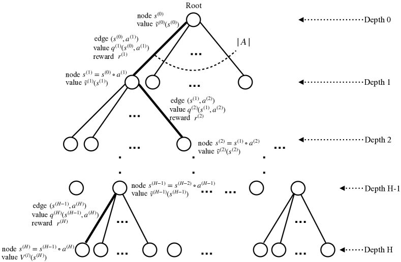
Figure 1: Notation and a sample simulation path of MCTS (thick lines).

We note that in selecting action $a^{(h+1)}$ at each depth $h$ (i.e., Line 6 of Algorithm 1), the upper confidence term is polynomial in $n$ while a typical UCB algorithm would be logarithmic in $n$, where $n$ is the number of visits to the corresponding state thus far. The logarithmic factor in the original UCB algorithm was motivated by the exponential tail probability bounds. In our case, it turns out that exponential tail bounds for each layer seems to be infeasible without further structural assumptions. As mentioned in Section 1.2, prior work (Audibert et al. 2009, Salomon and Audibert 2011) has justified the polynomial concentration of the regret for the classical UCB in stochastic (independent rewards) multi-arm bandit setting. This implies that the concentration at intermediate depth (i.e., depth less than $H$) is at most polynomial. Indeed, we will prove these polynomial concentration bounds even for non-stationary (dependent, non-stationary rewards) multi-arm bandit that show up in MCTS and discuss separately in Section 5.

3.2 Analysis

Now, we state the following result on the non-asymptotic performance of the MCTS as described above.

Theorem 1

Consider an MDP satisfying Assumption 1. Let $H\geq 1$, and for $1/2\leq\eta<1$, let

$$\eta^{(h)} =\eta^{(H)}\equiv\eta,\quad\forall\>h\in[H],$$ (6)

$$\alpha^{(h)} =\eta(1-\eta)\big{(}\alpha^{(h+1)}-1\big{)},\quad\forall\>h\in[H-1],$$ (7)

$$\xi^{(h)} =\alpha^{(h+1)}-1,\quad\forall h\in[H-1].$$ (8)

Suppose that a large enough $\xi^{(H)}$ is chosen such that $\alpha^{(1)}>2$. Then, there exist corresponding constants $\{\beta^{(i)}\}_{i=1}^{H}$ such that for each query state $s\in\mathcal{S},$ the following claim holds for the output $\hat{V}_{n}(s)$ of MCTS with $n$ simulations:

$$\Big{|}\mathbb{E}\big{[}\hat{V}_{n}(s)\big{]}-V^{*}(s)\Big{|}\leq\gamma^{H}\varepsilon_{0}+O\Big{(}n^{\eta-1}\Big{)},$$

where $\varepsilon_{0}=\|\hat{V}-V^{*}\|_{\infty}$ with $\hat{V}$ being the estimate of $V^{*}$ utilized by the MCTS algorithm for leaf nodes.

Since $\eta\in[1/2,1)$, Theorem 1 implies a best case convergence rate of $O(n^{-1/2})$ by setting $\eta=1/2$. With these parameter choices, the bias term in the upper confidence bound (line 6 of Algorithm 1) scales as $\big{(}N^{(h)}(s^{(h)})\big{)}^{1/4}/\sqrt{N^{(h+1)}(s^{(h)}\circ a)}$, that is, in the form of $t^{1/4}/\sqrt{S}$ as mentioned in the introduction, where $t\equiv N^{(h)}(s^{(h)})$ is the number of times that state $s^{(h)}$ at depth $h$ has been visited, and $S\equiv N^{(h+1)}(s^{(h)}\circ a)$ is the number of times action $a$ has been selected at state $s^{(h)}$.

4 Reinforcement Learning through MCTS with Supervised Learning

Recently, MCTS has been utilized prominently in various empirical successes of reinforcement learning including AlphaGo Zero (AGZ). Here, MCTS is combined with expressive supervised learning method to iteratively improve the policy as well as the value function estimation. In effect, MCTS combined with supervised learning acts as a “policy improvement” operator.

Intuitively, MCTS produces an improved estimation of value function for a given state of interest, starting with a given estimation of value function by “unrolling” the “computation tree” associated with value function iteration. And MCTS achieves this using observations obtained through simulations. Establishing this improvement property rigorously was the primary goal of Section 3. Now, given such improved estimation of value function for finitely many states, a good supervised learning method can learn to generalize such an improvement to all states. If so, this is like performing value function iteration, but using simulations. Presenting such a policy and establishing such guarantees is the crux of this section.

To that end, we present a reinforcement learning method that combines MCTS with nearest neighbor supervised learning. For this method, we establish that indeed, with sufficient number of samples, the resulting policy improves the value function estimation just like value function iteration. Using this, we provide a finite-sample analysis for learning the optimal value function within a given tolerance. We find it nearly matching a minimax lower bound in Shah and Xie (2018) which we recall in Section 4.4, and thus establishes near minimax optimality of such a reinforcement learning method.

4.1 Reinforcement Learning Policy

Here we describe the policy to produce estimation of optimal value function $V^{*}$. Similar approach can be applied to obtain estimation of policy as well. Let $V^{(0)}$ be the initial estimation of $V^{*}$, and for simplicity, let $V^{(0)}(\cdot)=0$. We describe a policy that iterates between use of MCTS and supervised learning to iteratively obtain estimation $V^{(\ell)}$ for $\ell\geq 1$, so that iteratively better estimation of $V^{*}$ is produced as $\ell$ increases. To that end, for $\ell\geq 1$,

• For appropriately sampled states $S^{\ell}=\{s_{i}\}_{i=1}^{m_{\ell}}$, apply MCTS to obtain improved estimations of value function $\{\hat{V}^{(\ell)}(s_{i})\}_{i=1}^{m_{\ell}}$ using $V^{(\ell-1)}$ to evaluate leaf nodes during simulations.

• Using $\{(s_{i},\hat{V}^{(\ell)}(s_{i})\}_{i=1}^{m_{\ell}}$ with a variant of nearest neighbor supervised learning with parameter $\delta_{\ell}\in(0,1)$, produce estimation $V^{(\ell)}$ of the optimal value function.

For completeness, the pseudo-code is provided in Algorithm 2.

Algorithm 2 Reinforcement Learning Policy

1:  Input: initial value function oracle $V^{(0)}(s)=0$, $\forall\>s\in\mathcal{S}$

2:  for $l=1,2,\dots,L$ do

3:     /*  improvement via MCTS  */

4:     uniformly and independently sample states $S^{\ell}=\{s_{i}\}_{i=1}^{m_{\ell}}$.

5:     for each sampled state $s_{i}$ do

6:        apply the MCTS algorithm, which takes as inputs the current value oracle $V^{(l-1)}$, the depth $H^{(l)}$, the number of simulation $n_{l}$, and the root node $s_{i}$, and outputs an improved estimate for $V^{*}(s_{i})$:

$$\vspace{-0.1in}\hat{V}^{(l)}(s_{i})=\textrm{MCTS}\big{(}V^{(l-1)},H^{(l)},n_{l},s_{i}\big{)}\vspace{-0.1in}$$ (9)

7:     end for

8:     /*  supervised learning  */

9:     with the collected data $\mathcal{D}^{(l)}=\{(s_{i},\hat{V}^{(l)}(s_{i}))\}_{i=1}^{m_{l}}$, build a new value oracle $V^{(l)}$ via a nearest neighbor regression with parameter $\delta_{l}$ :

$$\vspace{-0.1in}V^{(l)}(s)=\textrm{Nearest Neigbhor}\big{(}\mathcal{D}^{(l)},\delta_{l},s\big{)},\>\forall\>s\in\mathcal{S}.\vspace{-0.1in}$$ (10)

10:  end for

11:  Output: final value oracle $V^{(L)}$.

4.2 Supervised Learning

For simplicity, we shall utilize the following variant of the nearest neighbor supervised learning parametrized by $\delta\in(0,1)$. Given state space $\mathcal{S}=[0,1]^{d}$, we wish to cover it with minimal (up to scaling) number of balls of radius $\delta$ (with respect to $\ell_{2}$-norm). To that end, since $\mathcal{S}=[0,1]^{d}$, one such construction is where we have balls of radius $\delta$ with centers being $\{(\theta_{1},\theta_{2},\dots,\theta_{d}):\theta_{1},\dots,\theta_{d}\in{\mathcal{Q}}(\delta)\}$ where

$${\mathcal{Q}}(\delta)=\Big{\{}\frac{1}{2}\delta i~{}:~{}i\in\mathbb{Z},0\leq i\leq\Big{\lfloor}\frac{2}{\delta}\Big{\rfloor}\Big{\}}\cup\Big{\{}1-\frac{1}{2}\delta i~{}:~{}i\in\mathbb{Z},0\leq i\leq\Big{\lfloor}\frac{2}{\delta}\Big{\rfloor}\Big{\}}.$$

Let the collection of these balls be denoted by $c_{1},\dots,c_{K(\delta,d)}$ with $K(\delta,d)=|\mathcal{Q}(\delta)|$. It is easy to verify that $\mathcal{S}\subset\cup_{i\in[K(\delta,d)]}c_{i}$, $K(\delta,d)=\Theta(\delta^{-d})$ and $C_{d}\delta^{d}\leq{\sf volume}(c_{i}\cap\mathcal{S})\leq C^{\prime}_{d}\delta^{d}$ for strictly positive constants $C_{d},C^{\prime}_{d}$ that depends on $d$ but not $\delta$. For any $s\in\mathcal{S}$, let $j(s)=\min\{j:s\in c_{j}\}$. Given observations $\{(s_{i},\hat{V}^{(\ell)}(s_{i})\}_{i=1}^{m_{\ell}}$, we produce an estimate $V^{(\ell)}(s)$ for all $s\in\mathcal{S}$ as follows:

$$V^{(\ell)}(s) =\begin{cases}\frac{\sum_{i:s_{i}\in c_{j(s)}}\hat{V}^{(\ell)}(s_{i})}{|\{i:s_{i}\in c_{j(s)}\}|},&~{}~{}\mbox{if}~{}~{}|\{i:s_{i}\in c_{j(s)}\}|\neq 0,\\ 0&~{}~{}\mbox{otherwise.}\end{cases}$$ (11)

4.3 Finite-Sample Analysis

For finite-sample analysis of the proposed reinforcement learning policy, we make the following structural assumption about the MDP. Specifically, we assume that the optimal value function (i.e., true regression function) is smooth in some sense. We note that some form of smoothness assumption for MDPs with continuous state/action space is typical for $\ell_{\infty}$ guarantee. The Lipschitz continuous assumption stated below is natural and representative in the literature on MDPs with continuous state spaces, cf.  Munos et al. (2014), Dufour and Prieto-Rumeau (2012, 2013) and Bertsekas (1975).

Assumption 2 (Smoothness)

The optimal value function $V^{*}:\mathcal{S}\rightarrow\mathbb{R}$ satisfies Lipschitz continuity with parameter $C$, i.e., $\forall s,s^{\prime}\in\mathcal{S}=[0,1]^{d},$ $|V^{*}(s)-V^{*}(s^{\prime})|\leq C\|s-s^{\prime}\|_{2}.$

Now we state the result characterizing the performance of the reinforcement learning policy described above.

Theorem 2

Let Assumptions 1 and 2 hold. Let $\varepsilon>0$ be a given error tolerance. Then, for $L=\Theta\Big{(}\log\frac{\varepsilon}{V_{\max}}\Big{)}$, with appropriately chosen $m_{\ell},\delta_{\ell}$ for $\ell\in[L]$ as well as parameters in MCTS, the reinforcement learning algorithm produces estimation of value function $V^{(L)}$ such that

$$\mathbb{E}\big{[}\sup_{s\in\mathcal{S}}|V^{(L)}(s)-V^{*}(s)|\big{]}\leq\varepsilon,$$

by selecting $m_{\ell}$ states uniformly at random in $\mathcal{S}$ within iteration $\ell$. This, in total, requires T number of state transitions (or samples), where

$$T =O\Big{(}\varepsilon^{-\big{(}4+d\big{)}}\cdot\big{(}\log{\frac{1}{\varepsilon}}\big{)}^{5}\Big{)}.$$

4.4 Minimax Lower Bound

Leveraging the the minimax lower bound for the problem of non-parametric regression (Tsybakov 2009, Stone 1982), recent work Shah and Xie (2018) establishes a lower bound on the sample complexity for reinforcement learning algorithms for general MDPs without additional structural assumptions. Indeed the lower bound also holds for MDPs with deterministic transitions (the proof is provided in Appendix 10), which is stated in the following proposition.

Proposition 1

Given an algorithm, let $V_{T}$ be the estimation of $V^{*}$ after $T$ samples of state transitions for the given MDP. Then, for each $\varepsilon\in(0,1)$, there exists an instance of deterministic MDP such that in order to achieve $\mathbb{P}\big{[}\big{\|}\hat{V}_{T}-V^{*}\big{\|}_{\infty}<\varepsilon\big{]}\geq 1-\varepsilon,$ it must be that

$$T\geq C^{\prime}d\cdot\varepsilon^{-(d+2)}\cdot\log(\varepsilon^{-1}),$$

where $C^{\prime}>0$ is a constant independent of the algorithm.

Proposition 1 states that for any policy to learn the optimal value function within $\varepsilon$ approximation error, the number of samples required must scale as $\widetilde{\Omega}\big{(}{\varepsilon^{-(2+d)}}\big{)}$. Theorem 2 implies that the sample complexity of the proposed algorithm scales as $\widetilde{O}\big{(}{\varepsilon^{-(4+d)}}\big{)}$ (omitting the logarithmic factor). Hence, in terms of the dependence on the dimension, the proposed algorithm is nearly optimal. Optimizing the dependence of the sample complexity on other parameters is an important direction for future work.

5 Non-stationary Multi-Arm Bandit

We introduce a class of non-stationary multi-arm bandit (MAB) problems, which will play a crucial role in analyzing the MCTS algorithm. To that end, let there be $K\geq 1$ arms or actions of interest. Let $X_{i,t}$ denote the random reward obtained by playing the arm $i\in[K]$ for the $t$th time with $t\geq 1$. Let $\bar{X}_{i,n}=\frac{1}{n}\sum_{t=1}^{n}X_{i,t}$ denote the empirical average of playing arm $i$ for $n$ times, and let $\mu_{i,n}=\mathbb{E}[\bar{X}_{i,n}]$ be its expectation. For each arm $i\in[K]$, the reward $X_{i,t}$ is bounded in $[-R,R]$ for some $R>0$, and we assume that the reward sequence, $\{X_{i,t}:t\geq 1\}$, is a non-stationary process satisfying the following convergence and concentration properties:

1. (Convergence) the expectation $\mu_{i,n}$ converges to a value $\mu_{i}$, i.e.,

   $$\mu_{i}=\lim_{n\rightarrow\infty}\mathbb{E}[\bar{X}_{i,n}].$$ (12)

2. (Concentration) there exist three constants, $\beta>1$, $\xi>0$, and $1/2\leq\eta<1$ such that for every $z\geq 1$ and every integer $n\geq 1$,

   $$\mathbb{P}\big{(}n\bar{X}_{i,n}-n\mu_{i} \geq n^{\eta}z\big{)}\leq\frac{\beta}{z^{\xi}},~{}~{}\mathbb{P}\big{(}n\bar{X}_{i,n}-n\mu_{i}\leq-n^{\eta}z\big{)}\leq\frac{\beta}{z^{\xi}}.$$ (13)

5.1 Algorithm

Consider applying the following variant of Upper Confidence Bound (UCB) algorithm to the above non-stationary MAB. Define upper confidence bound for arm or action $i$ when it is played $s$ times in total of $t\geq s$ time steps as

$$U_{i,s,t} =\bar{X}_{i,s}+B_{t,s},$$ (14)

where $B_{t,s}$ is the “bonus term”. Denote by $I_{t}$ the arm played at time $t\geq 1$. Then,

$$I_{t}\in\arg\max_{i\in[K]}\big{\{}\bar{X}_{i,T_{i}(t-1)}+B_{t-1,T_{i}(t-1)}\big{\}},$$ (15)

where $T_{i}(t)=\sum_{l=1}^{t}\mathbb{I}{\{I_{l}=i\}}$ is the number of times arm $i$ has been played, up to (including) time $t$. We shall make specific selection of the bonus or bias term $B_{t,s}$ as

$$B_{t,s}=\frac{\beta^{1/\xi}\cdot t^{\alpha/\xi}}{s^{1-\eta}}.$$ (16)

A tie is broken arbitrarily when selecting an arm. In the above, $\alpha>0$ is a tuning parameter that controls the exploration and exploitation trade-off. Let $\mu_{*}=\max_{i\in[K]}\mu_{i}$ be the optimal value with respect to the converged expectation, and $i_{*}\in\arg\max_{i\in[K]}\mu_{i}$ be the corresponding optimal arm. We assume that the optimal arm is unique. Let $\delta_{i*,n}=\mu_{i_{*},n}-\mu_{i_{*}}$, which measures how fast the mean of the optimal non-stationary arm converges. For simplicity, quantities related to the optimal arm $i_{*}$ will be simply denoted with subscript $*$, e.g., $\delta_{*},n=\delta_{i_{*},n}$. Finally, denote by $\Delta_{\min}=\min_{i\in[K],i\neq i_{*}}\Delta_{i}$ the gap between the optimal arm and the second optimal arm with notation $\Delta_{i}=\mu_{*}-\mu_{i}$.

5.2 Analysis

Let $\bar{X}_{n}\triangleq\frac{1}{n}\sum_{i=1}^{K}T_{i}(n)\bar{X}_{i,T_{i}(n)}$ denote the empirical average under the UCB algorithm (15). Then, $\bar{X}_{n}$ satisfies the following convergence and concentration properties.

Theorem 3

Consider a non-stationary MAB satisfying (12) and (13). Suppose that algorithm (15) is applied with parameter $\alpha$ such that $\xi\eta(1-\eta)\leq\alpha<\xi(1-\eta)$ and $\alpha>2$. Then, the following holds:

1. Convergence:

   $$\left|\mathbb{E}[\bar{X}_{n}]-\mu_{*}\right| \leq|\delta_{*,n}|+\frac{2R(K-1)\cdot\Big{(}\big{(}\frac{2}{\Delta_{\min}}\cdot\beta^{1/\xi}\big{)}^{\frac{1}{1-\eta}}\cdot n^{\frac{\alpha}{\xi(1-\eta)}}+\frac{2}{\alpha-2}+1\Big{)}}{n}.$$

2. Concentration: there exist constants, $\beta^{\prime}>1$ and $\xi^{\prime}>0$ and $1/2\leq\eta^{\prime}<1$ such that for every $n\geq 1$ and every $z\geq 1$,

   $$\mathbb{P}\big{(}n\bar{X}_{n}-n\mu_{*} \geq n^{\eta^{\prime}}z\big{)}\leq\frac{\beta^{\prime}}{z^{\xi^{\prime}}},~{}~{}~{}\mathbb{P}\big{(}n\bar{X}_{n}-n\mu_{*}\leq-n^{\eta^{\prime}}z\big{)}\leq\frac{\beta^{\prime}}{z^{\xi^{\prime}}},$$

   where $\eta^{\prime}=\frac{\alpha}{\xi(1-\eta)}$, $\xi^{\prime}=\alpha-1$, $\beta^{\prime}$ depends on $R,K,\Delta_{\min},\beta,$ $\xi,\alpha,\eta$.

6 Proof of Theorem 3

We establish the convergence and concentration properties of the variant of the Upper Confidence Bound algorithm described in Section 5 and specified through (14), (15) and (16).

Establishing the Convergence Property. We define a useful notation

$$\Phi(n,\delta)=n^{\eta}\bigg{(}\frac{\beta}{\delta}\bigg{)}^{1/\xi}.$$ (17)

We begin with a useful lemma, which shows that the probability that a non-optimal arm or action has a large upper confidence is polynomially small. Proof is provided in Section 6.1.

Lemma 1

Let $i\in[K],i\neq i_{*}$ be a sub-optimal arm and define

$$A_{i}(t) \triangleq\min_{u\in\mathbb{N}}\Big{\{}\frac{\Phi(u,t^{-\alpha})}{u}\leq\frac{\Delta_{i}}{2}\Big{\}}=\bigg{\lceil}\Big{(}\frac{2}{\Delta_{i}}\cdot\beta^{1/\xi}\cdot t^{\alpha/\xi}\Big{)}^{\frac{1}{1-\eta}}\bigg{\rceil}.$$ (18)

For each $s$ and $t$ such that, $A_{i}(t)\leq s\leq t$, we have

$$\mathbb{P}(U_{i,s,t}>\mu_{*})\leq t^{-\alpha}.$$

Lemma 1 implies that as long as each arm is played enough, the sub-optimal ones become less likely to be selected. This allows us to upper bound the expected number of sub-optimal plays as follows.

Lemma 2

Let $i\in[K],i\neq i_{*}$, then

$$\mathbb{E}[T_{i}(n)]\leq\Big{(}\frac{2}{\Delta_{i}}\cdot\beta^{1/\xi}\Big{)}^{\frac{1}{1-\eta}}\cdot n^{\frac{\alpha}{\xi(1-\eta)}}+\frac{2}{\alpha-2}+1.$$

Proof of Lemma 2 is deferred to Section 6.2.

Completing Proof of Convergence. By the triangle inequality,

$$\left|\mu_{*}-\mathbb{E}[\bar{X}_{n}]\right|=\left|\mu_{*}-\mu_{*,n}\right|+\left|\mu_{*,n}-\mathbb{E}[\bar{X}_{n}]\right|=\left|\delta_{*,n}\right|+\left|\mu_{*,n}-\mathbb{E}[\bar{X}_{n}]\right|.$$

The second term can be bounded as follows:

$$n\left|\mu_{*,n}-\mathbb{E}[\bar{X}_{n}]\right|$$

$$=\Bigg{|}\mathbb{E}\bigg{[}\sum_{t=1}^{n}X_{i_{*},t}\bigg{]}-\mathbb{E}\bigg{[}\sum_{i=1}^{K}T_{i}(n)\bar{X}_{i,T_{i}(n)}\bigg{]}\Bigg{|}$$

$$\leq\Bigg{|}\mathbb{E}\bigg{[}\sum_{t=1}^{n}X_{i_{*},t}\bigg{]}-\mathbb{E}\bigg{[}T_{*}(n)\bar{X}_{i_{*},T_{*}(n)}\bigg{]}\Bigg{|}+\Bigg{|}\mathbb{E}\bigg{[}\sum_{i=1,i\neq i_{*}}^{K}T_{i}(n)\bar{X}_{i,T_{i}(n)}\bigg{]}\Bigg{|}$$

$$=\Bigg{|}\mathbb{E}\bigg{[}\sum_{t=T_{*}(n)+1}^{n}X_{i_{*},t}\bigg{]}\Bigg{|}+\Bigg{|}\mathbb{E}\bigg{[}\sum_{i=1,i\neq i_{*}}^{K}T_{i}(n)\bar{X}_{i,T_{i}(n)}\bigg{]}\Bigg{|}.$$ (19)

Recall that the reward sequences are assumed to be bounded in $[-R,R]$. Therefore, the first term of (19) can be bounded as follows:

$$\Bigg{|}\mathbb{E}\bigg{[}\sum_{t=T_{*}(n)+1}^{n}X_{i_{*},t}\bigg{]}\Bigg{|}\leq\mathbb{E}\bigg{[}\sum_{t=T_{*}(n)+1}^{n}|X_{i_{*},t}|\bigg{]}\leq R\cdot\mathbb{E}\bigg{[}\sum_{i=1,i\neq i_{*}}^{K}T_{i}(n)\bigg{]}.$$

The second term can also be bounded as:

$$\Bigg{|}\mathbb{E}\bigg{[}\sum_{i=1,i\neq i_{*}}^{K}T_{i}(n)\bar{X}_{i,T_{i}(n)}\bigg{]}\Bigg{|} \leq R\cdot\mathbb{E}\bigg{[}\sum_{i=1,i\neq i_{*}}^{K}T_{i}(n)\bigg{]}.$$

Hence, we obtain that

$$\left|\mu_{*}-\mathbb{E}[\bar{X}_{n}]\right|=\left|\delta_{*,n}\right|+\left|\mu_{*,n}-\mathbb{E}[\bar{X}_{n}]\right|\leq\left|\delta_{*,n}\right|+\frac{2R\cdot\mathbb{E}\big{[}\sum_{i=1,i\neq i_{*}}^{K}T_{i}(n)\big{]}}{n}.$$

Combining the above bounds and Lemma 2 yields the desired convergence result in Theorem 3.

Establishing the Concentration Property. Having proved the convergence property, the next step is to show that a similar concentration property (cf. (13)) also holds for $\bar{X}_{n}$. We aim to precisely capture the relationship between the original constants assumed in the assumption and the new constants obtained for $\bar{X}_{n}$. To begin with, recall the definition of $A_{i}(t)$ in Lemma 1 and define

$$A(t) =\max_{i\in[K]}A_{i}(t)=\bigg{\lceil}\Big{(}\frac{2}{\Delta_{\min}}\cdot\beta^{1/\xi}\Big{)}^{\frac{1}{1-\eta}}\cdot t^{\frac{\alpha}{\xi(1-\eta)}}\bigg{\rceil}.$$ (20)

It can be checked that replacing $\beta$ with any larger number still makes the concentration inequalities (13) hold. Without loss of generality, we hence let $\beta$ be large enough so that $\frac{2}{\Delta_{\min}}\cdot\beta^{1/\xi}>1$. We further denote by $N_{p}$ the first time such that $t\geq A(t)$, i.e.,

$$N_{p} =\min\{t\geq 1\>:\>t\geq A(t)\}~{}=~{}\Theta\Big{(}\big{(}\frac{2^{\xi}\beta}{\Delta_{\min}^{\xi}}\big{)}^{\frac{1}{\xi(1-\eta)-\alpha}}\Big{)}.$$ (21)

We first state the following concentration property, which will be further refined to match the desired form in Theorem 3. We defer the proof to Section 6.3.

Lemma 3

For any $n\geq N_{p}$ and $x\geq 1$, let $r_{0}=n^{\eta}+2R(K-1)\big{(}3+A(n)\big{)}.$ Then,

$$\mathbb{P}\Big{(}n\bar{X}_{n}-n\mu_{*}\geq r_{0}x\Big{)}\leq\frac{\beta}{x^{\xi}}+\frac{2(K-1)}{(\alpha-1)\big{(}(1+A(n))x\big{)}^{\alpha-1}},$$

$$\mathbb{P}\Big{(}n\bar{X}_{n}-n\mu_{*}\leq-r_{0}x\Big{)}\leq\frac{\beta}{x^{\xi}}+\frac{2(K-1)}{(\alpha-1)\big{(}(1+A(n))x\big{)}^{\alpha-1}}.$$

Lemma 3 confirms that indeed, as $n$ becomes large, the average $\bar{X}_{n}$ also satisfies certain concentration inequalities. However, the particular form of concentration in Theorem 3 does not quite match the form of concentration in Theorem 3 which we conclude next.

Completing Proof of Concentration Property. Let $N_{p}^{\prime}$ be a constant defined as follows:

$$N_{p}^{\prime}=\min\{t\geq 1:t\geq A(t)\textrm{ and }2RA(t)\geq t^{\eta}+2R(4K-3)\}.$$

Recall the definition of $A(t)$ and that $\alpha\geq\xi\eta(1-\eta)$ and $\alpha<\xi(1-\eta)$. Hence, $N_{p}^{\prime}$ is guaranteed to exist. In addition, note that by definition, $N_{p}^{\prime}\geq N_{p}$. For each $n\geq N_{p}^{\prime}$,

$$2RK\Big{(}\frac{2}{\Delta_{\min}}\cdot\beta^{1/\xi}\Big{)}^{\frac{1}{1-\eta}}\cdot n^{\frac{\alpha}{\xi(1-\eta)}} =2RK\Big{[}\Big{(}\frac{2}{\Delta_{\min}}\cdot\beta^{1/\xi}\Big{)}^{\frac{1}{1-\eta}}\cdot n^{\frac{\alpha}{\xi(1-\eta)}}+1-1\Big{]}$$

$$\geq 2RKA(n)-2RK$$

$$=2R(K-1)A(n)+2RA(n)-2RK$$

$$\geq 2R(K-1)A(n)+n^{\eta}+2R(4K-3)-2RK$$

$$=2R(K-1)(A(n)+3)+n^{\eta}=r_{0}$$

Now, let us apply Lemma 3: for every $n\geq N_{p}^{\prime}$ and $x\geq 1$, we have

$$\mathbb{P}\Big{(}n\bar{X}_{n}-n\mu_{*}\geq n^{\frac{\alpha}{\xi(1-\eta)}}\Big{[}2RK\Big{(}\frac{2}{\Delta_{\min}}\cdot\beta^{1/\xi}\Big{)}^{\frac{1}{1-\eta}}\Big{]}x\Big{)} \leq\mathbb{P}\Big{(}n\bar{X}_{n}-n\mu_{*}\geq r_{0}x\Big{)}$$

$$\leq\frac{\beta}{x^{\xi}}+\frac{2(K-1)}{(\alpha-1)\big{(}(1+A(n))x\big{)}^{\alpha-1}}$$

$$\leq\frac{2\max(\beta,\frac{2(K-1)}{(\alpha-1)(1+A(N_{p}^{\prime}))^{\alpha-1}})}{x^{\alpha-1}},$$ (22)

where the last inequality follows because $n\geq N_{p}^{\prime}$ and $A(n)$ is a non-decreasing function. In addition, since $\alpha<\xi(1-\eta)<\xi$, we have $\alpha-1<\xi$. For convenience, we define a constant

$$c_{1}\triangleq 2RK\Big{(}\frac{2}{\Delta_{\min}}\cdot\beta^{1/\xi}\Big{)}^{\frac{1}{1-\eta}}.$$ (23)

Equivalently, by a change of variable, i.e., letting $z=c_{1}x$, then for every $n\geq N_{p}^{\prime}$ and $z\geq 1$, we obtain that

$$\mathbb{P}\Big{(}n\bar{X}_{n}-n\mu_{*}\geq n^{\frac{\alpha}{\xi(1-\eta)}}z\Big{)} \leq\frac{2c_{1}^{\alpha-1}\cdot\max\big{(}\beta,\frac{2(K-1)}{(\alpha-1)(1+A(N_{p}^{\prime}))^{\alpha-1}}\big{)}}{z^{\alpha-1}}.$$ (24)

The above inequality holds because: (1) if $z\geq c_{1}$, then (24) directly follows from (22); (2) if $1\leq z\leq c_{1}$, then the R.H.S. of (24) is at least 1 (by assumption, $\beta>1$) and the inequality trivially holds. The concentration inequality, i.e., Eq. (24), is now almost the same as the desired form in Theorem 3. The only difference is that it only holds for $n\geq N_{p}^{\prime}$. This is not hard to resolve. The easiest approach, which we show in the following, is to refine the constants to ensure that when $1\leq n<N_{p}^{\prime}$, Eq. (24) is trivially true. To this end, we note that $|n\bar{X}_{n}-n\mu_{*}|\leq 2Rn$. For each $1\leq n<N_{p}^{\prime}$, there is a corresponding $\bar{z}(n)$ such that $n^{\frac{\alpha}{\xi(1-\eta)}}\bar{z}(n)=2Rn$. That is,

$$\bar{z}(n)\triangleq 2Rn^{1-\frac{\alpha}{\xi(1-\eta)}},\quad 1\leq n<N_{p}^{\prime}.$$

This then implies that for each $1\leq n<N_{p}^{\prime}$, the following inequality trivially holds:

$$\mathbb{P}\Big{(}n\bar{X}_{n}-n\mu_{*}\geq n^{\frac{\alpha}{\xi(1-\eta)}}z\Big{)}\leq\frac{\bar{z}(n)^{\alpha-1}}{z^{\alpha-1}},\quad\forall\>z\geq 1.$$

To see why, note that for each $1\leq n<N_{p}^{\prime}$: (1) if $z\geq\bar{z}(n)$, then $n^{\frac{\alpha}{\xi(1-\eta)}}z\geq 2Rn$ and the above probability should be $0$. Hence, any positive number on the R.H.S. makes the inequality trivially true; (2) if $1\leq z<\bar{z}(n)$, the R.H.S. is at least 1, which again makes the inequality hold. For convenience, define

$$c_{2}\triangleq\max_{1\leq n<N_{p}^{\prime}}\bar{z}(n)=2R(N_{p}^{\prime}-1)^{1-\frac{\alpha}{\xi(1-\eta)}}.$$ (25)

Then, it is easy to see that for every $n\geq 1$ and every $z\geq 1$, we have

$$\mathbb{P}\big{(}n\bar{X}_{n}-n\mu_{*}\geq n^{\eta^{\prime}}z\big{)}\leq\frac{\beta^{\prime}}{z^{\xi^{\prime}}},$$

where the constants are given by

$$\eta^{\prime} =\frac{\alpha}{\xi(1-\eta)},$$ (26)

$$\xi^{\prime} =\alpha-1,$$ (27)

$$\beta^{\prime} =\max\Big{\{}c_{2},\>2c_{1}^{\alpha-1}\cdot\max\big{(}\beta,\frac{2(K-1)}{(\alpha-1)(1+A(N_{p}^{\prime}))^{\alpha-1}}\big{)}\Big{\}}.$$ (28)

Finally, notice that since $\alpha\geq\xi\eta(1-\eta)$ and $\alpha<\xi(1-\eta)$, we have $1/2\leq\eta\leq\eta^{\prime}<1$. Note that per (23), $c_{1}$ depends on $R,K,\Delta_{\min},\beta,\xi$ and $\eta$. In addition, $c_{2}$ depends on $R,K,\Delta_{\min},\beta,\xi,\alpha,\eta$ and $N_{p}^{\prime}$ depends on $R,K,\Delta_{\min},\beta,\xi,\alpha,\eta$. Therefore, $\beta^{\prime}$ depends on $R,K,\Delta_{\min},\beta,$ $\xi,\alpha,\eta$. The other direction follows exactly the same reasoning, and this completes the proof of Theorem 3.

6.1 Proof of Lemma  1

By the choice of $A_{i}(t)$, $s$ and $t$, we have $B_{t,s}=\frac{\Phi(s,t^{-\alpha})}{s}\leq\frac{\Phi(A_{i}(t),t^{-\alpha})}{A_{i}(t)}\leq\frac{\Delta_{i}}{2}$. Therefore,

$$\mathbb{P}(U_{i,s,t}>\mu_{*}) =\mathbb{P}(\bar{X}_{i,s}+B_{t,s}>\mu_{*})$$

$$=\mathbb{P}\bigg{(}\bar{X}_{i,s}-\mu_{i}>\Delta_{i}-B_{t,s}\bigg{)}$$

$$\leq\mathbb{P}\bigg{(}\bar{X}_{i,s}-\mu_{i}>B_{t,s}\bigg{)} \Delta_{i}\geq 2B_{t,s}$$

$$\leq t^{-\alpha}. \text{by concentration (\ref{eq:nonstmab.conc})}.$$

6.2 Proof of Lemma 2

If a sub-optimal arm $i$ is chosen at time $t+1$, i.e., $I_{t+1}=i$, then at least one of the following two equations must be true: with notation $T_{*}(\cdot)=T_{i_{*}}(\cdot$),

$$U_{i_{*},T_{*}(t),t} \leq\mu_{*}\;,$$ (29)

$$U_{i,T_{i}(t),t} >\mu_{*}\;.$$ (30)

Indeed, if both inequalities are false, we have $U_{i_{*},T_{*}(t),t}>\mu_{*}\geq U_{i,T_{i}(t),t}$, which is a contradiction to $I_{t+1}=i$. We now use this fact to prove Lemma 2.

Case 1: $n>A_{i}(n)$. Note that such $n$ exists because $A_{i}(n)$ grows with a polynomial order $O\big{(}n^{\frac{\alpha}{\xi(1-\eta)}}\big{)}$ and $\alpha<\xi(1-\eta)$, i.e., $A_{i}(n)=o(n)$. Then,

$$T_{i}(n) =\sum_{t=0}^{n-1}\mathbb{I}\{I_{t+1}=i\}\stackrel{{\scriptstyle(a)}}{{=}}1+\sum_{t=K}^{n-1}\mathbb{I}\{I_{t+1}=i\}$$

$${=}1+\sum_{t=K}^{n-1}\big{(}\mathbb{I}\{I_{t+1}=i,T_{i}(t)<A_{i}(n)\}+\mathbb{I}\{I_{t+1}=i,T_{i}(t)\geq A_{i}(n)\}\big{)}$$

$$\leq A_{i}(n)+\sum_{t=K}^{n-1}\mathbb{I}\{I_{t+1}=i,T_{i}(t)\geq A_{i}(n)\},$$

where equality (a) follows from the fact that $B_{t,s}=\infty$ if $s=0$.

To analyze the above summation, we note that from (29) and (30),

$$\mathbb{I}\{I_{t+1}=i,T_{i}(t)\geq A_{i}(n)\} \leq\mathbb{I}\{U_{i_{*},T_{*}(t),t}\leq\mu_{*}\text{ or }U_{i,T_{i}(t),t}>\mu_{*},T_{i}(t)\geq A_{i}(n)\}$$

$$\leq\mathbb{I}\{U_{i,T_{i}(t),t}>\mu_{*},T_{i}(t)\geq A_{i}(n)\}+\mathbb{I}\{U_{i_{*},T_{*}(t),t}\leq\mu_{*},T_{i}(t)\geq A_{i}(n)\}$$

$$\leq\mathbb{I}\{U_{i,T_{i}(t),t}>\mu_{*},T_{i}(t)\geq A_{i}(n)\}+\mathbb{I}\{U_{i_{*},T_{*}(t),t}\leq\mu_{*}\}$$

$$=\mathbb{I}\{\exists\>s:A_{i}(n)\leq s\leq t,\text{ s.t. }U_{i,s,t}>\mu_{*}\}+\mathbb{I}\{\exists\>s_{*}:1\leq s_{*}\leq t,\text{ s.t. }U_{i_{*},s_{*},t}\leq\mu_{*}\}.$$

To summarize, we have proved that

$$\mathbb{E}[T_{i}(n)] \leq A_{i}(n)+\sum_{t=A_{i}(n)}^{n-1}\mathbb{P}\Big{(}(\ref{eq:Uopt_bound})\text{ or }(\ref{eq:Ui_bound})\text{ is true}\text{, and }T_{i}(t)\geq A_{i}(n)\Big{)}$$

$$\leq A_{i}(n)+\sum_{t=A_{i}(n)}^{n-1}\Big{[}\mathbb{P}\big{(}\underbrace{\exists\>s:A_{i}(n)\leq s\leq t,\text{ s.t. }U_{i,s,t}>\mu_{*}}_{E_{1}}\big{)}+\mathbb{P}\big{(}\underbrace{\exists\>s_{*}:1\leq s_{*}\leq t,\text{ s.t. }U_{i_{*},s_{*},t}\leq\mu_{*}}_{E_{2}}\big{)}\Big{]}.$$ (31)

To complete the proof of Lemma 2, it suffices to bound the probabilities of the two events $E_{1}$ and $E_{2}$. To this end, we use a union bound:

$$\mathbb{P}\big{(}E_{1}\big{)} \leq\sum_{s=A_{i}(n)}^{t}\mathbb{P}\big{(}U_{i,s,t}>\mu_{*}\big{)}\overset{(a)}{\leq}\sum_{s=A_{i}(n)}^{t}t^{-\alpha}\leq t\cdot t^{-\alpha}=t^{1-\alpha},$$

where the step $(a)$ follows from $A_{i}(n)\geq A_{i}(t)$ and Lemma 1. We bound $\mathbb{P}(E_{2})$ in a similar way:

$$\mathbb{P}(E_{2}) \leq\sum_{s_{*}=1}^{t}\mathbb{P}(U_{i_{*},s_{*},t}\leq\mu_{*})=\sum_{s_{*}=1}^{t}\mathbb{P}\bigg{(}\bar{X}_{i_{*},s_{*}}+B_{t,s_{*}}\leq\mu_{*}\bigg{)}\overset{(a)}{\leq}\sum_{s_{*}=1}^{t}t^{-\alpha}\leq t^{1-\alpha},$$

where step $(a)$ follows from concentration (cf. (13)). By substituting the bounds of $\mathbb{P}(E_{1})$ and $\mathbb{P}(E_{2})$ into (31), we have:

$$\mathbb{E}[T_{i}(n)] \leq A_{i}(n)+\sum_{t=A_{i}(n)}^{n-1}2t^{1-\alpha}$$

$$\leq A_{i}(n)+\int_{A_{i}(n)-1}^{\infty}2t^{1-\alpha}dt \alpha>2$$

$$=A_{i}(n)+\frac{2\big{(}A_{i}(n)-1\big{)}^{2-\alpha}}{\alpha-2}$$

$$\leq A_{i}(n)+\frac{2}{\alpha-2}$$

$$\leq\Big{(}\frac{2}{\Delta_{i}}\cdot\beta^{1/\xi}\Big{)}^{\frac{1}{1-\eta}}\cdot n^{\frac{\alpha}{\xi(1-\eta)}}+\frac{2}{\alpha-2}+1.$$

Case 2: $n\leq A_{i}(n)$. Note that if $n$ is such that $n\leq A_{i}(n)$, then the above bound trivially holds because $T_{i}(n)\leq n\leq A_{i}(n)$. This completes the proof of Lemma 2.

6.3 Proof of Lemma 3

We first prove one direction, namely, $\mathbb{P}(n\mu_{*}-n\bar{X}_{n}\geq r_{0}x)$. The other direction follows the similar steps, and we will comment on that at the end of this proof. The general idea underlying the proof is to rewrite the quantity $n\mu_{*}-n\bar{X}_{n}$ as sums of terms that can be bounded using previous lemmas or assumptions. To begin with, note that

$$n\mu_{*}-n\bar{X}_{n} =n\mu_{*}-\sum_{i=1}^{K}T_{i}(n)\bar{X}_{i,T_{i}(n)}$$

$$=n\mu_{*}-\sum_{t=1}^{T_{*}(n)}X_{i_{*},t}-\sum_{i\neq i_{*}}T_{i}(n)\bar{X}_{i,T_{i}(n)}$$

$$=n\mu_{*}-\sum_{t=1}^{n}X_{i_{*},t}+\sum_{t=T_{*}(n)+1}^{n}X_{i_{*},t}-\sum_{i\neq i_{*}}\sum_{t=1}^{T_{i}(n)}X_{i,t}$$

$$\leq n\mu_{*}-\sum_{t=1}^{n}X_{i_{*},t}+2R\sum_{i\neq i_{*}}T_{i}(n),$$

because $X_{i,t}\in[-R,R]$ for all $i,t$. Therefore, we have

$$\mathbb{P}\big{(}n\mu_{*}-n\bar{X}_{n}\geq r_{0}x\big{)} \leq\mathbb{P}\big{(}n\mu_{*}-\sum_{t=1}^{n}X_{i_{*},t}+2R\sum_{i\neq i_{*}}T_{i}(n)\geq r_{0}x\big{)}$$

$$\leq\mathbb{P}\big{(}n\mu_{*}-\sum_{t=1}^{n}X_{i_{*},t}\geq n^{\eta}x\big{)}+\sum_{i\neq i_{*}}\mathbb{P}\big{(}T_{i}(n)\geq{(3+A(n))x}\big{)},$$ (32)

where the last inequality follows from the union bound.

To prove the theorem, we now bound the two terms in (32). By our concentration assumption, we can upper bound the first term as follows:

$$\mathbb{P}\big{(}n\mu_{*}-\sum_{t=1}^{n}X_{i_{*},t}\geq n^{\eta}x\big{)}\leq\frac{\beta}{x^{\xi}}.$$ (33)

Next, we bound each term in the summation of (32). Fix $n$ and a sub-optimal edge $i$. Let $u$ be an integer satisfying $u\geq A(n).$ For any $\tau\in\mathbb{R}$, consider the following two events:

$$E_{1} =\big{\{}\text{For each integer }t\in[u,n],\text{ we have }U_{i,u,t}\leq\tau\big{\}},$$

$$E_{2} =\big{\{}\text{For each integer }s\in[1,n-u],\text{ we have }U_{i_{*},s,u+s}>\tau\big{\}}.$$

As a first step, we want to show that

$$E_{1}\cap E_{2}\Rightarrow T_{i}(n)\leq u.$$ (34)

To this end, let us condition on both events $E_{1}$ and $E_{2}$. Recall that $B_{t,s}$ is non-decreasing with respect to $t$. Then, for each $s$ such that $1\leq s\leq n-u,$ and each $t$ such that $u+s\leq t\leq n$, it holds that

$$U_{i_{*},s,t}=\bar{X}_{i_{*},s}+B_{t,s}\geq\bar{X}_{i_{*},s}+B_{u+s,s}=U_{i_{*},s,u+s}>\tau\geq U_{i,u,t}.$$

This implies that $T_{i}(n)\leq u$. To see why, suppose that $T_{i}(n)>u$ and denote by $t^{\prime}$ the first time that arm $i$ has been played $u$ times, i.e., $t^{\prime}=\min\{t:t\leq n,T_{i}(t)=u\}$. Note that by definition $t^{\prime}\geq u+T_{*}(t^{\prime})$. Hence, for any time t such that $t^{\prime}<t\leq n$, the above inequality implies that $U_{i_{*},T_{*}(t),t}>U_{i,u,t}$. That is, $i^{*}$ always has a higher upper confidence bound than $i$, and arm $i$ will not be selected, i.e., arm $i$ will not be played the $(u+1)$-th time. This contradicts our assumption that $T_{i}(n)>u$, and hence we have the inequality $T_{i}(n)\leq u$.

To summarize, we have established the fact that $E_{1}\cap E_{2}\Rightarrow T_{i}(n)\leq u.$ As a result, we have:

$$\{T_{i}(n)>u\} \subset\big{(}E_{1}^{c}\cup E_{2}^{c}\big{)}=\big{(}\big{\{}\exists\>t:\ u\leq t\leq n\text{ s.t. }U_{i,u,t}>\tau\big{\}}\cup\big{\{}\exists\>s:\text{}1\leq s\leq n-u,\text{ s.t. }U_{i_{*},s,u+s}\leq\tau\big{\}}\big{)}.$$

Using union bound, we obtain that

$$\mathbb{P}\big{(}T_{i}(n)>u\big{)}\leq\sum_{t=u}^{n}\mathbb{P}(U_{i,u,t}>\tau)+\sum_{s=1}^{n-u}\mathbb{P}\big{(}U_{i_{*},s,u+s}\leq\tau\big{)}.$$ (35)

Note that for the above bound, we are free to choose $u$ and $\tau$ as long as $u\geq A(n)$. To connect with our goal (cf. (32)), in the following, we set $u=\lfloor(1+A(n))x\rfloor+1$ (recall that $x\geq 1$) and $\tau=\mu_{*}$ to bound $\mathbb{P}(T_{i}(n)>u).$ Since $u\geq A(n)\geq A_{i}(n)$, by Lemma 1, we have

$$\sum_{t=u}^{n}\mathbb{P}(U_{i,u,t}>\mu_{*})\leq\sum_{t=u}^{n}t^{-\alpha}\leq\int_{u-1}^{\infty}t^{-\alpha}dt =\frac{(u-1)^{1-\alpha}}{\alpha-1}$$

$$=\frac{(\lfloor(1+A(n))x\rfloor)^{1-\alpha}}{\alpha-1}\leq\frac{\Big{(}(1+A(n))x\Big{)}^{1-\alpha}}{\alpha-1}.$$

As for the second summation in the R.H.S. of (35), we have that

$$\sum_{s=1}^{n-u}\mathbb{P}\big{(}U_{i_{*},s,u+s}\leq\tau\big{)} =\sum_{s=1}^{n-u}\mathbb{P}(U_{i_{*},s,u+s}\leq\mu_{*})$$

$$=\sum_{s=1}^{n-u}\mathbb{P}\bigg{(}\bar{X}_{i_{*},s}+B_{u+s,s}\leq\mu_{*}\bigg{)}$$

$$\leq\sum_{s=1}^{n-u}(s+u)^{-\alpha}=\sum_{t=1+u}^{n}t^{-\alpha}$$

$$\leq\int_{u-1}^{\infty}t^{-\alpha}dt=\frac{(u-1)^{1-\alpha}}{\alpha-1}\leq\frac{\Big{(}(1+A(n))x\Big{)}^{1-\alpha}}{\alpha-1},$$

where the first inequality follows from the concentration property, cf. (13). Combining the above inequalities and note that $(3+A(n))x>\lfloor(1+A(n))x\rfloor+1$:

$$\mathbb{P}\big{(}T_{i}(n)\geq(3+A(n))x\big{)}\leq\mathbb{P}\big{(}T_{i}(n)>u\big{)}\leq\frac{2\Big{(}\big{(}1+A(n)\big{)}x\Big{)}^{1-\alpha}}{\alpha-1}.$$ (36)

Substituting (33) and (36) into (32), we obtain

$$\mathbb{P}\big{(}n\mu_{*}-n\bar{X}_{n}\geq r_{0}x\big{)}\leq\frac{\beta}{x^{\xi}}+\sum_{i\neq i_{*}}\frac{2\Big{(}\big{(}1+A(n)\big{)}x\Big{)}^{1-\alpha}}{\alpha-1},$$

which is the desired inequality in Lemma 3.

To complete the proof, we need to consider the other direction, i.e., $\mathbb{P}(n\bar{X}_{n}-n\mu_{*}\geq r_{0}x)$. The proof is almost identical. Note that

$$n\bar{X}_{n}-n\mu_{*} =\sum_{i=1}^{K}T_{i}(n)\bar{X}_{i,T_{i}(n)}-n\mu_{*}$$

$$=\sum_{t=1}^{n}X_{i_{*},t}-n\mu_{*}-\sum_{t=T_{*}(n)+1}^{n}X_{i_{*},t}+\sum_{i\neq i_{*}}\sum_{t=1}^{T_{i}(n)}X_{i,t}$$

$$\leq\sum_{t=1}^{n}X_{i_{*},t}-n\mu_{*}+2R\sum_{i\neq i_{*}}T_{i}(n),$$

because $X_{i,t}\in[-R,R]$ for all $i,t$. Therefore,

$$\mathbb{P}\big{(}n\bar{X}_{n}-n\mu_{*}\geq r_{0}x\big{)} \leq\mathbb{P}\big{(}\sum_{t=1}^{n}X_{i_{*},t}-n\mu_{*}+2R\sum_{i\neq i_{*}}T_{i}(n)\geq r_{0}x\big{)}$$

$$\leq\mathbb{P}\big{(}\sum_{t=1}^{n}X_{i_{*},t}-n\mu_{*}\geq n^{\eta}x\big{)}+\sum_{i\neq i_{*}}\mathbb{P}\big{(}T_{i}(n)\geq(3+A_{i}(n))x\big{)}.$$

The desired inequality then follows exactly from the same reasoning of our previous proof.

7 Analysis of MCTS and Proof of Theorem 1

In this section, we give a complete analysis for the fixed-depth Monte Carlo Tree Search (MCTS) algorithm illustrated in Algorithm 1 and prove Theorem 1. In effect, as discussed in Section 3, one can view a depth-$H$ MCTS as a simulated version of $H$ steps value function iterations. Given the current value function proxy $\hat{V}$, let $V^{(H)}(\cdot)$ be the value function estimation after $H$ steps of value function iteration starting with the proxy $\hat{V}$. Then, we prove the result in two parts. First, we argue that due to the MCTS sampling process, the mean of the empirical estimation of value function at the query node $s$, or the root node of MCTS tree, is within $O(n^{\eta-1})$ of $V^{(H)}(s)$ after $n$ simulations, with the given proxy $\hat{V}$ being the input to the MCTS algorithm. Second, we argue that $V^{(H)}(s)$ is within $\gamma^{H}\|\hat{V}-V^{*}\|_{\infty}\leq\gamma^{H}\varepsilon_{0}$ of the optimal value function. Putting this together leads to Theorem 1.

We start by a preliminary probabilistic lemma in Section 7.1 that will be useful throughout. Sections 7.2 and 7.3 argue the first part of the proof as explained above. Section 7.4 provides proof of the second part. And Section 7.5 concludes the proof of Theorem 1.

7.1 Preliminary

We state the following probabilistic lemma that is useful throughout. Proof can be found in Section 7.6.

Lemma 4

Consider real-valued random variables $X_{i},Y_{i}$ for $i\geq 1$ such that $X$s are independent and identically distributed taking values in $[-B,B]$ for some $B>0$, $X$s are independent of $Y$s, and $Y$s satisfy

1. Convergence: for $n\geq 1$, with notation $\bar{Y}_{n}=\frac{1}{n}\big{(}\sum_{i=1}^{n}Y_{i}\big{)}$,

   $$\lim_{n\to\infty}\mathbb{E}[\bar{Y}_{n}] =\mu_{Y}.$$

2. Concentration: there exist constants, $\beta>1$, $\xi>0$, $1/2\leq\eta<1$ such that for $n\geq 1$ and $z\geq 1$,

   $$\mathbb{P}\big{(}n\bar{Y}_{n}-n\mu_{Y}\geq n^{\eta}z\big{)}\leq\frac{\beta}{z^{\xi}},\quad\mathbb{P}\big{(}n\bar{Y}_{n}-n\mu_{Y}\leq-n^{\eta}z\big{)}\leq\frac{\beta}{z^{\xi}}.$$

Let $Z_{i}=X_{i}+\rho Y_{i}$ for some $\rho>0$. Then, $Z$s satisfy

1. Convergence: for $n\geq 1$, with notation $\bar{Z}_{n}=\frac{1}{n}\big{(}\sum_{i=1}^{n}Z_{i}\big{)}$, and $\mu_{X}=\mathbb{E}[X_{1}]$,

   $$\lim_{n\to\infty}\mathbb{E}[\bar{Z}_{n}] =\mu_{X}+\rho\mu_{Y}.$$

2. Concentration: there exist constant $\beta^{\prime}>1$ depending upon $\rho,\xi,\beta$ and $B$, such that for $n\geq 1$ and $z\geq 1$,

   $$\mathbb{P}\big{(}n\bar{Z}_{n}-n(\mu_{X}+\rho\mu_{Y})\geq n^{\eta}z\big{)}\leq\frac{\beta^{\prime}}{z^{\xi}},\quad\mathbb{P}\big{(}n\bar{Z}_{n}-n(\mu_{X}+\rho\mu_{Y})\leq-n^{\eta}z\big{)}\leq\frac{\beta^{\prime}}{z^{\xi}}.$$

7.2 Analyzing Leaf Level $H$

The goal is to understand the empirical reward observed at the query node for MCTS or the root node of the MCTS tree. In particular, we argue that the mean of the empirical reward at the root node of the MCTS tree is within $O(n^{\eta-1})$ of the mean reward obtained at it assuming access to infinitely many samples. We start by analyzing the reward collected at the nodes that are at leaf level $H$ and level $H-1$.

The nodes at leaf level, i.e., level $H$, are children of nodes at level $H-1$ in the MCTS tree. Let there be $n_{H-1}$ nodes at level $H-1$ corresponding to states $s_{1,H-1},\dots,s_{n_{H-1},H-1}\in\mathcal{S}$. Consider node $i\in[n_{H-1}]$ at level $H-1$, corresponding to state $s_{i,H-1}$. As part of the algorithm, whenever this node is visited, one of the $K$ feasible actions is taken. When an action $a\in[K]$ is taken, the node $s^{\prime}_{H}=s_{i,H-1}\circ a$, at the leaf level $H$ is reached. This results in reward at node $s_{i,H-1}$ (at level $H-1$) being equal to $\mathcal{R}(s_{i,H-1},a)+\gamma\tilde{v}^{(H)}(s^{\prime}_{H})$. Here, for each $s\in\mathcal{S}$ and $a\in[K]$, the reward $\mathcal{R}(s,a)$ is an independent, bounded random variable taking value in $[-R_{\max},R_{\max}]$ with distribution dependent on $s,a$; $\tilde{v}^{(H)}(\cdot)$ is the input of value function proxy to the MCTS algorithm denoted as $\hat{V}(\cdot)$, and $\gamma\in[0,1)$ is the discount factor. Recall that $\varepsilon_{0}=\|\hat{V}-V^{*}\|_{\infty}$ and $\|V^{*}\|_{\infty}\leq V_{\max}$. Therefore, $\|\tilde{v}^{(H)}\|_{\infty}=\|\hat{V}\|_{\infty}\leq V_{\max}+\varepsilon_{0}$, and the reward collected at node $s_{i,H-1}$ by following any action is bounded, in absolute value, by $\tilde{R}_{\max}^{(H-1)}=R_{\max}+\gamma(V_{\max}+\varepsilon_{0})$.

As part of the MCTS algorithm as described in (5), when node $s_{i,H-1}$ is visited for the $t+1$ time with $t\geq 0$, the action taken is

$$\arg\max_{a\in\mathcal{A}} \bigg{\{}\frac{1}{u_{a}}\sum_{j=1}^{u_{a}}\Big{(}r(s_{i,H-1},a)(j)+\gamma\tilde{v}^{(H)}(s_{i,H-1}\circ a)(j)\Big{)}+\frac{\big{(}\beta^{(H)}\big{)}^{1/\xi^{(H)}}\cdot\big{(}t\big{)}^{\alpha^{(H)}/\xi^{(H)}}}{\big{(}u_{a}\big{)}^{1-\eta^{(H)}}}\bigg{\}},$$

where $u_{a}\leq t$ is the number of times action $a$ has been chosen thus far at state $s_{i,H-1}$ in the $t$ visits so far, $r(s_{i,H-1},a)(j)$ is the $j$th sample of random variable per distribution $\mathcal{R}(s_{i,H-1},a)$, and $\tilde{v}^{(H)}(s_{i,H-1}\circ a)(j)$ is the reward evaluated at leaf node $s_{i,H-1}\circ a$ for the $j$th time. Note that for all $j$, the reward evaluated at leaf node $s_{i,H-1}\circ a$ is the same and equals to $\tilde{v}^{(H)}(\cdot)$, the input value function proxy for the algorithm. When $u_{a}=0$, we use notation $\infty$ to represent quantity inside the $\arg\max$. The net discounted reward collected by node $s_{i,H-1}$ during its total of $t\geq 1$ visits is simply the sum of rewards obtained by selecting the actions per the policy – which includes the reward associated with taking an action and the evaluation of $\tilde{v}^{(H)}(\cdot)$ for appropriate leaf node, discounted by $\gamma$. In effect, at each node $s_{i,H-1}$, we are using the UCB policy described in Section 5 with parameters $\alpha^{(H)},\beta^{(H)},\xi^{(H)},\eta^{(H)}$ with $K$ possible actions, where the rewards collected by playing any of these $K$ actions each time is simply the summation of bounded independent and identical (for a given action) random variable and a deterministic evaluation. By applying Lemma 4, where $X$s correspond to independent rewards, $\rho=\gamma$, and $Y$s correspond to deterministic evaluations of $\tilde{v}^{(H)}(\cdot)$, we obtain that for given $\xi^{(H)}>0$ and $\eta^{(H)}\in[\frac{1}{2},1)$, there exists $\beta^{(H)}$ such that the collected rewards at $s_{i,H-1}$ (i.e., sum of i.i.d. reward and deterministic evaluations) satisfy the convergence property cf. (12) and concentration property cf. (13) stated in Section 5. Therefore, by an application of Theorem 3, we conclude Lemma 5 stated below. We define some notations first:

$$\mu^{(H-1)}_{a}(s_{i,H-1}) =\mathbb{E}[\mathcal{R}(s_{i,H-1},a)]+\gamma\tilde{v}^{(H)}(s_{i,H-1}\circ a),$$

$$\mu^{(H-1)}_{*}(s_{i,H-1}) =\max_{a\in[K]}\mu^{(H-1)}_{a}(s_{i,H-1})$$

$$a^{(H-1)}_{*}(s_{i,H-1}) \in\arg\max_{a\in[K]}\mu^{(H-1)}_{a}(s_{i,H-1})$$ (37)

$$\Delta^{(H-1)}_{\min}(s_{i,H-1}) =\mu^{(H-1)}_{*}(s_{i,H-1})-\max_{a\neq a^{(H-1)}_{*}(s_{i,H-1})}\mu^{(H-1)}_{a}(s_{i,H-1}).$$

We shall assume that the maximizer in the set $\arg\max_{a\in[K]}\mu^{(H-1)}_{a}(s_{i,H-1})$ is unique, i.e. $\Delta_{\min}^{(H-1)}(s_{i,H-1})>0$. And further note that all rewards belong to $[-\tilde{R}_{\max}^{(H-1)},\tilde{R}_{\max}^{(H-1)}]$.

Lemma 5

Consider a node corresponding to state $s_{i,H-1}$ at level $H-1$ within the MCTS for $i\in[n_{H-1}]$. Let $\tilde{v}^{(H-1)}(s_{i,H-1})_{n}$ be the total discounted reward collected at $s_{i,H-1}$ during $n\geq 1$ visits of it, to one of its $K$ leaf nodes under the UCB policy. Then, for the choice of appropriately large $\beta^{(H)}>0$, for a given $\xi^{(H)}>0$, $\eta^{(H)}\in[\frac{1}{2},1)$ and $\alpha^{(H)}>2$, we have

1. Convergence:

   $$\left|\mathbb{E}\Big{[}\frac{1}{n}\tilde{v}^{(H-1)}(s_{i,H-1})_{n}\Big{]}-\mu^{(H-1)}_{*}(s_{i,H-1})\right|$$

   $$\leq\frac{2\tilde{R}_{\max}^{(H-1)}(K-1)\cdot\Big{(}\big{(}\frac{2(\beta^{(H)})^{\frac{1}{\xi^{(H)}}}}{\Delta^{(H-1)}_{\min}(s_{i,H-1})}\big{)}^{\frac{1}{1-\eta^{(H)}}}\cdot n^{\frac{\alpha^{(H)}}{\xi^{(H)}(1-\eta^{(H)})}}+\frac{2}{\alpha^{(H)}-2}+1\Big{)}}{n}.$$

2. Concentration: there exist constants, $\beta^{\prime}>1$ and $\xi^{\prime}>0$ and $1/2\leq\eta^{\prime}<1$ such that for every $n\geq 1$ and every $z\geq 1$,

   $$\mathbb{P}\big{(}\tilde{v}^{(H-1)}(s_{i,H-1})_{n}-n\mu^{(H-1)}_{*}(s_{i,H-1})\geq n^{\eta^{\prime}}z\big{)}\leq\frac{\beta^{\prime}}{z^{\xi^{\prime}}},$$

   $$\mathbb{P}\big{(}\tilde{v}^{(H-1)}(s_{i,H-1})_{n}-n\mu^{(H-1)}_{*}(s_{i,H-1})\leq-n^{\eta^{\prime}}z\big{)}\leq\frac{\beta^{\prime}}{z^{\xi^{\prime}}},$$

   where $\eta^{\prime}=\frac{\alpha^{(H)}}{\xi^{(H)}(1-\eta^{(H)})}$, $\xi^{\prime}=\alpha^{(H)}-1$, and $\beta^{\prime}$ is a large enough constant that is function of parameters $\alpha^{(H)},\beta^{(H)},\xi^{(H)},$ $\eta^{(H)},\tilde{R}_{\max}^{(H-1)},K,\Delta^{(H-1)}_{\min}(s_{i,H-1})$.

Let $\Delta_{\min}^{(H-1)}=\min_{i\in[n_{H-1}]}\Delta^{(H-1)}_{\min}(s_{i,H-1})$. Then, the rate of convergence for each node $s_{i,H-1}$, $i\in[n_{H-1}]$ can be uniformly simplified as

$$\delta^{(H-1)}_{n}= \frac{2\tilde{R}_{\max}^{(H-1)}(K-1)\cdot\Big{(}\big{(}\frac{2(\beta^{(H)})^{\frac{1}{\xi^{(H)}}}}{\Delta_{\min}^{(H-1)}}\big{)}^{\frac{1}{1-\eta^{(H)}}}\cdot n^{\frac{\alpha^{(H)}}{\xi^{(H)}(1-\eta^{(H)})}}+\frac{2}{\alpha^{(H)}-2}+1\Big{)}}{n}$$

$$= ~{}\Theta\Big{(}n^{\frac{\alpha^{(H)}}{\xi^{(H)}(1-\eta^{(H)})}-1}\Big{)}$$

$$\stackrel{{\scriptstyle(a)}}{{=}} ~{}O\big{(}n^{\eta-1}\big{)},$$

where (a) holds since $\alpha^{(H)}=\xi^{(H)}(1-\eta^{(H)})\eta^{(H)},~{}\eta^{(H)}=\eta$. It is worth remarking that $\mu^{(H-1)}_{*}(s_{i,H-1})$, as defined in (37), is precisely the value function estimation for $s_{i,H-1}$ at the end of one step of value iteration starting with $\hat{V}$.

7.3 Recursion: Going From Level $h$ to $h-1$.

Lemma 5 suggests that the necessary assumption of Theorem 3, i.e. (12) and (13), are satisfied by $\tilde{v}^{(H-1)}_{n}$ for each node or state at level $H-1$, with $\alpha^{(H-1)},\xi^{(H-1)},\eta^{(H-1)}$ as defined per relationship (6) - (8) and with appropriately defined large enough constant $\beta^{(H-1)}$. We shall argue that result similar to Lemma 5, but for node at level $H-2$, continues to hold with parameters $\alpha^{(H-2)},\xi^{(H-2)},\eta^{(H-2)}$ as defined per relationship (6) - (8) and with appropriately defined large enough constant $\beta^{(H-2)}$. And similar argument will continue to apply going from level $h$ to $h-1$ for all $h\leq H-1$. That is, we shall assume that the necessary assumption of Theorem 3, i.e. (12) and (13), holds for $\tilde{v}^{(h)}(\cdot)$, for all nodes at level $h$ with $\alpha^{(h)},\xi^{(h)},\eta^{(h)}$ as defined per relationship (6) - (8) and with appropriately defined large enough constant $\beta^{(h)}$, and then argue that such holds for nodes at level $h-1$ as well. This will, using mathematical induction, allow us to prove the results for all $h\geq 1$.

To that end, consider any node at level $h-1$. Let there be $n_{h-1}$ nodes at level $h-1$ corresponding to states $s_{1,h-1},\dots,s_{n_{h-1},h-1}\in\mathcal{S}$. Consider a node corresponding to state $s_{i,h-1}$ at level $h-1$ within the MCTS for $i\in[n_{h-1}].$ As part of the algorithm, whenever this node is visited, one of the $K$ feasible action is taken. When an action $a\in[K]$ is taken, the node $s^{\prime}_{h}=s_{i,h-1}\circ a$, at the level $h$ is reached. This results in reward at node $s_{i,h-1}$ at level $h-1$ being equal to $\mathcal{R}(s_{i,h-1},a)+\gamma\tilde{v}^{(h)}(s^{\prime}_{h})$. As noted before, $\mathcal{R}(s,a)$ is an independent, bounded valued random variable while $\tilde{v}^{(h)}(\cdot)$ is effectively collected by following a path all the way to the leaf level. Inductively, we assume that $\tilde{v}^{(h)}(\cdot)$ satisfies the convergence and concentration property for each node or state at level $h$, with $\alpha^{(h)},\xi^{(h)},\eta^{(h)}$ as defined per relationship (6) - (8) and with appropriately defined large enough constant $\beta^{(h)}$. Therefore, by an application of Lemma 4, it follows that this combined reward continues to satisfy (12) and (13), with $\alpha^{(h)},\xi^{(h)},\eta^{(h)}$ as defined per relationship (6) - (8) and with a large enough constant which we shall denote as $\beta^{(h)}$. These constants are used by the MCTS policy. By an application of Theorem 3, we can obtain the following Lemma 6 regarding the convergence and concentration properties for the reward sequence collected at node $s_{i,h-1}$ at level $h-1.$ Similar to the notation in Eq. (37), let

$$\mu^{(h-1)}_{a}(s_{i,h-1}) =\mathbb{E}[\mathcal{R}(s_{i,h-1},a)]+\gamma\mu^{(h)}_{*}(s_{i,h-1}\circ a)$$

$$\mu^{(h-1)}_{*}(s_{i,h-1}) =\max_{a\in[K]}\mu^{(h-1)}_{a}(s_{i,h-1})$$

$$a^{(h-1)}_{*}(s_{i,h-1}) \in\arg\max_{a\in[K]}\mu^{(h-1)}_{a}(s_{i,h-1})$$ (38)

$$\Delta^{(h-1)}_{\min}(s_{i,h-1}) =\mu^{(h-1)}_{*}(s_{i,h-1})-\max_{a\neq a^{(h-1)}_{*}(s_{i,h-1})}\mu^{(h-1)}_{a}(s_{i,h-1}).$$

Again, we shall assume that the maximizer in the set $\arg\max_{a\in[K]}\mu^{(h-1)}_{a}(s_{i,h-1})$ is unique, i.e. $\Delta^{(h-1)}_{\min}(s_{i,h-1})>0$. Define $\tilde{R}_{\max}^{(h-1)}=R_{\max}+\gamma\tilde{R}_{\max}^{(h)},$ where $\tilde{R}^{(H)}=V_{\max}+\varepsilon_{0}.$ Note that all rewards collected at level $h-1$ belong to $[-\tilde{R}^{(h-1)}_{\max},\tilde{R}^{(h-1)}_{\max}]$.

Lemma 6

Consider a node corresponding to state $s_{i,h-1}$ at level $h-1$ within the MCTS for $i\in[n_{h-1}]$. Let $\tilde{v}^{(h-1)}(s_{i,h-1})_{n}$ be the total discounted reward collected at $s_{i,h-1}$ during $n\geq 1$ visits. Then, for the choice of appropriately large $\beta^{(h)}>0$, for a given $\xi^{(h)}>0$, $\eta^{(h)}\in[\frac{1}{2},1)$ and $\alpha^{(h)}>2$, we have

1. Convergence:

   $$\left|\mathbb{E}\Big{[}\frac{1}{n}\tilde{v}^{(h-1)}(s_{i,h-1})_{n}\Big{]}-\mu^{(h-1)}_{*}(s_{i,h-1})\right|$$

   $$\leq\frac{2\tilde{R}_{\max}^{(h-1)}(K-1)\cdot\Big{(}\big{(}\frac{2(\beta^{(h)})^{\frac{1}{\xi^{(h)}}}}{\Delta^{(h-1)}_{\min}(s_{i,h-1})}\big{)}^{\frac{1}{1-\eta^{(h)}}}\cdot n^{\frac{\alpha^{(h)}}{\xi^{(h)}(1-\eta^{(h)})}}+\frac{2}{\alpha^{(h)}-2}+1\Big{)}}{n}.$$

2. Concentration: there exist constants, $\beta^{\prime}>1$ and $\xi^{\prime}>0$ and $1/2\leq\eta^{\prime}<1$ such that for $n\geq 1$, $z\geq 1$,

   $$\mathbb{P}\big{(}\tilde{v}^{(h-1)}(s_{i,h-1})_{n}-n\mu^{(h-1)}_{*}(s_{i,h-1})\geq n^{\eta^{\prime}}z\big{)}\leq\frac{\beta^{\prime}}{z^{\xi^{\prime}}},$$

   $$\mathbb{P}\big{(}\tilde{v}^{(h-1)}(s_{i,h-1})_{n}-n\mu^{(h-1)}_{*}(s_{i,h-1})\leq-n^{\eta^{\prime}}z\big{)}\leq\frac{\beta^{\prime}}{z^{\xi^{\prime}}},$$

   where $\eta^{\prime}=\frac{\alpha^{(h)}}{\xi^{(h)}(1-\eta^{(h)})}$, $\xi^{\prime}=\alpha^{(h)}-1$, and $\beta^{\prime}$ is a large enough constant that is function of parameters $\alpha^{(h)},\beta^{(h)},\xi^{(h)},$ $\eta^{(h)},\tilde{R}_{\max}^{(h-1)},K,\Delta^{(h-1)}_{\min}(s_{i,h-1})$.

As before, let us define $\Delta_{\min}^{(h-1)}=\min_{i\in[n_{h-1}]}\Delta^{(h-1)}_{\min}(s_{i,h-1})$. Similarly, we can show that for every node $s_{i,h-1}$, $i\in[n_{h-1}]$, the rate of convergence in Lemma 6 can be uniformly simplified as

$$\delta^{(h-1)}_{n} =\frac{2\tilde{R}_{\max}^{(h-1)}(K-1)\cdot\Big{(}\big{(}\frac{2(\beta^{(h)})^{\frac{1}{\xi^{(h)}}}}{\Delta_{\min}^{(h-1)}}\big{)}^{\frac{1}{1-\eta^{(h)}}}\cdot n^{\frac{\alpha^{(h)}}{\xi^{(h)}(1-\eta^{(h)})}}+\frac{2}{\alpha^{(h)}-2}+1\Big{)}}{n}$$

$$~{}=~{}\Theta\Big{(}n^{\frac{\alpha^{(h)}}{\xi^{(h)}(1-\eta^{(h)})}-1}\Big{)}~{}=~{}O\big{(}n^{\eta-1}\big{)},$$

where the last equality holds as $~{}\alpha^{(h)}=\xi^{(h)}(1-\eta^{(h)})\eta^{(h)}$ and $~{}\eta^{(h)}=\eta.$ Again, it is worth remarking, inductively, that $\mu^{(h-1)}_{*}(s_{i,h-1})$ is precisely the value function estimation for $s_{i,h-1}$ at the end of $H-h+1$ steps of value iteration starting with $\hat{V}$.

Remark (Recursive Relation among Parameters). With the above development, we are ready to elaborate our choice of parameters in Theorem 1, defined recursively via Eqs. (6)-(8). In essence, those parameter requirements originate from our analysis of the non-stationary MAB, i.e., Theorem 3. Recall that from our previous analysis, the key to establish the MCTS guarantee is to recursively argue the convergence and the polynomial concentration properties at each level; that is, we recursively solve the non-stationary MAB problem at each level. In order to do so, we apply our result on the non-stationary MAB (Theorem 3) recursively at each level. Importantly, recall that Theorem 3 only holds when $\xi\eta(1-\eta)\leq\alpha<\xi(1-\eta)$ and $\alpha>2$, under which it leads to the recursive conclusions $\eta^{\prime}=\frac{\alpha}{\xi(1-\eta)}$ and $\xi^{\prime}=\alpha-1$. Using our notation with superscript indicating the levels, this means that apart from the parameters at the leaf level (level $H$) which could be freely chosen, we must choose parameters of other levels recursively so that the following conditions hold:

$$\alpha^{(h)}>2,\quad\xi^{(h)}\eta^{(h)}(1-\eta^{(h)})\leq\alpha^{(h)}<\xi^{(h)}(1-\eta^{(h)}),$$

$$\xi^{(h)}=\alpha^{(h+1)}-1\textrm{ and }\eta^{(h)}=\frac{\alpha^{(h+1)}}{\xi^{(h+1)}(1-\eta^{(h+1)})}.$$

It is not hard to see that the conditions in Theorem 1 guarantee the above. There might be other sequences of parameters satisfying the requirements, but our particular choice gives cleaner analysis as presented in this paper.

7.4 Error Analysis for Value Function Iteration

We now move to the second part of the proof. The value function iteration improves the estimation of optimal value function by iterating Bellman equation. In effect, the MCTS tree is “unrolling” $H$ steps of such an iteration. Precisely, let $V^{(h)}(\cdot)$ denote the value function after $h$ iterations starting with $V^{(0)}=\hat{V}$. By definition, for any $h\geq 0$ and $s\in\mathcal{S}$,

$$V^{(h+1)}(s) =\max_{a\in[K]}\Big{(}\mathbb{E}[\mathcal{R}(s,a)]+\gamma V^{(h)}(s\circ a)\Big{)}.$$ (39)

Recall that value iteration is contractive with respect to $\|\cdot\|_{\infty}$ norm (cf. Bertsekas (2017)). That is, for any $h\geq 0$,

$$\|V^{(h+1)}-V^{*}\|_{\infty} \leq\gamma\|V^{(h)}-V^{*}\|_{\infty}.$$ (40)

As remarked earlier, $\mu^{(h-1)}_{*}(s_{i,h-1})$, the mean reward collected at node $s_{i,h-1}$ for $i\in[n_{h-1}]$ for any $h\geq 1$, is precisely $V^{(H-h+1)}(s_{i,h-1})$ starting with $V^{(0)}=\hat{V}$, the input to MCTS policy. Therefore, the mean reward collected at root node $s^{(0)}$ of the MCTS tree satisfies $\mu^{(0)}_{*}(s^{(0)})=V^{(H)}(s^{(0)})$. Using (40), we obtain the following Lemma.

Lemma 7

The mean reward collected under the MCTS policy at root note $s^{(0)}$, $\mu^{(0)}_{*}(s^{(0)})$, starting with input value function proxy $\hat{V}$ is such that

$$|\mu^{(0)}_{*}(s^{(0)})-V^{*}(s^{(0)})| \leq\gamma^{H}\|\hat{V}-V^{*}\|_{\infty}.$$ (41)

7.5 Completing Proof of Theorem 1

In summary, using Lemma 6, we conclude that the recursive relationship going from level $h$ to $h-1$ holds for all $h\geq 1$ with level $0$ being the root. At root $s^{(0)}$, the query state that is input to the MCTS policy, we have that after $n$ total simulations of MCTS, the empirical average of the rewards over these $n$ trial, $\frac{1}{n}\tilde{v}^{(0)}(s_{0})_{n}$ is such that (using the fact that $\alpha^{(0)}=\xi^{(0)}(1-\eta^{(0)})\eta^{(0)}$)

$$\left|\mathbb{E}\Big{[}\frac{1}{n}\tilde{v}^{(0)}(s_{0})_{n}\Big{]}-\mu^{(0)}_{*}\right| =O\Big{(}n^{\frac{\alpha^{(0)}}{\xi^{(0)}(1-\eta^{(0)})}-1}\Big{)}~{}=~{}O\Big{(}n^{\eta-1}\Big{)},$$ (42)

where $\mu^{(0)}_{*}$ is the value function estimation for $s^{(0)}$ after $H$ iterations of value function iteration starting with $\hat{V}$. By Lemma 7, we have

$$|\mu^{(0)}_{*}-V^{*}(s^{(0)})| \leq\gamma^{H}\varepsilon_{0},$$ (43)

since $\varepsilon_{0}=\|\hat{V}-V^{*}\|_{\infty}$. Combining (42) and (43),

$$\left|\mathbb{E}\Big{[}\frac{1}{n}\tilde{v}^{(0)}(s_{0})_{n}\Big{]}-V^{*}(s^{(0)})\right| \leq\gamma^{H}\varepsilon_{0}+O\Big{(}n^{\eta-1}\Big{)}.$$ (44)

This concludes the proof of Theorem 1.

7.6 Proof of Lemma 4

The convergence property, $\lim_{n\to\infty}\mathbb{E}[\bar{Z}_{n}]=\mu_{X}+\rho\mu_{Y}$, follows simply by linearity of expectation. For concentration, consider the following: since $X$s are i.i.d. bounded random variables taking value in $[-B,B]$, by Hoeffding’s inequality (Hoeffding 1963), we have that for $t\geq 0$,

$$\mathbb{P}\big{(}n\bar{X}_{n}-n\mu_{X}\geq nt\big{)}\leq\exp\Big{(}-\frac{t^{2}n}{2B^{2}}\Big{)},$$ (45)

$$\mathbb{P}\big{(}n\bar{X}_{n}-n\mu_{X}\leq-nt\big{)}\leq\exp\Big{(}-\frac{t^{2}n}{2B^{2}}\Big{)}.$$

Therefore,

$$\mathbb{P}\Big{(}n\bar{Z}_{n}-n(\mu_{X}+\rho\mu_{Y})\geq n^{\eta}z\big{)} \leq\mathbb{P}\Big{(}n\bar{X}_{n}-n\mu_{X}\geq\frac{n^{\eta}z}{2}\Big{)}+\mathbb{P}\Big{(}n\bar{Y}_{n}-n\mu_{Y}\geq\frac{n^{\eta}z}{2\rho}\Big{)}$$

$$\leq\exp\Big{(}-\frac{z^{2}n^{2\eta-1}}{8B^{2}}\Big{)}+\frac{\beta 2^{\xi}\rho^{\xi}}{z^{\xi}}$$

$$\leq\frac{\beta^{\prime}}{z^{\xi}},$$ (46)

where $\beta^{\prime}$ is a large enough constant depending upon $\rho,\xi,\beta$ and $B$. The other-side of the inequality follows similarly. This completes the proof.

8 Proof of Theorem 2

First, we establish a useful property of nearest neighbor supervised learning presented in Section 4.2. This is stated in Section 8.1. We will use it, along with the guarantees obtained for MCTS in Theorem 1 to establish Theorem 2 in Section 8.2. Throughout, we shall assume the setup of Theorem 2.

8.1 Guarantees for Supervised Learning

Let $\delta\in(0,1)$ be given. As stated in Section 4.2, let $K(\delta,d)=\Theta(\delta^{-d})$ be the collection of balls of radius $\delta$, say $c_{i},~{}i\in[K(\delta,d)]$, so that they cover $\mathcal{S}$, i.e. $\mathcal{S}\subset\cup_{i\in[K(\varepsilon,d)]}c_{i}$. Also, by construction, each of these balls have intersection with $\mathcal{S}$ whose volume is at least $C_{d}\delta^{d}$. Let $S=\{s_{i}:i\in[N]\}$ denote $N$ state samples from $\mathcal{S}$ uniformly at random and independent of each other. For each state $s\in\mathcal{S}$, let $V:\mathcal{S}\to[-{V_{\max},V_{\max}}]$ be such that $|\mathbb{E}[V(s)]-V^{*}(s)|\leq\Delta$. Let the nearest neighbor supervised learning described in Section 4.2 produce estimate $\hat{V}:\mathcal{S}\to\mathbb{R}$ using labeled data points $(s_{i},V(s_{i}))_{i\in[N]}$. Then, we claim the following guarantee. Proof can be found in Section 8.3.

Lemma 8

Under the above described setup, as long as $N\geq 32\max(1,\delta^{-2}V_{\max}^{2})C_{d}^{-1}\delta^{-d}\log\frac{K(\delta,d)}{\delta}$, i.e., $N=\Omega(d\delta^{-d-2}\log\delta^{-1})$,

$$\mathbb{E}\big{[}\sup_{s\in\mathcal{S}}|\hat{V}(s)-V^{*}(s)|\big{]} \leq\Delta+(C+1)\delta+\frac{{4V_{\max}}\delta^{2}}{K(\delta,d)}.$$ (47)

8.2 Establishing Theorem 2

Using Theorem 1 and Lemma 8, we complete the proof of Theorem 2 under appropriate choice of algorithmic parameters. We start by setting some notation.

To that end, the algorithm as described in Section 4.1 iterates between MCTS and supervised learning. In particular, let $\ell\geq 1$ denote the iteration index. Let $m_{\ell}$ be the number of states that are sampled uniformly at random, independently, over $\mathcal{S}$ in this iteration, denoted as $S^{(\ell)}=\{s_{i}^{(\ell)}:i\in[m_{\ell}]\}$. Let $V^{(\ell-1)}$ be the input of value function from prior iteration, using which the MCTS algorithm with $n_{\ell}$ simulations obtains improved estimates of value function for states in $S^{(\ell)}$ denoted as $\hat{V}^{(\ell)}(s_{i}^{(\ell)}),~{}i\in[m_{\ell}]$. Using $(s_{i}^{(\ell)},\hat{V}^{(\ell)}(s_{i}^{(\ell)}))_{i\in[m_{\ell}]}$, the nearest neighbor supervised learning as described above with balls of appropriate radius $\delta_{\ell}\in(0,1)$ produces estimate $V^{(\ell)}$ for all states in $\mathcal{S}$. Let $\mathcal{F}^{(\ell)}$ denote the smallest $\sigma$-algebra containing all information pertaining to the algorithm (both MCTS and supervised learning). Define the error under MCTS in iteration $\ell$ as

$$\varepsilon_{\text{mcts}}^{(\ell)} =\mathbb{E}\big{[}\sup_{s\in\mathcal{S}}\big{|}\mathbb{E}\big{[}\hat{V}^{(\ell)}(s)\big{|}\mathcal{F}^{(\ell-1)}\big{]}-V^{*}(s)\big{|}\big{]}.$$ (48)

And, the error for supervised learning in iteration $\ell$ as

$$\theta_{\text{sl}}^{(\ell)} =\sup_{s\in\mathcal{S}}\big{|}V^{(\ell)}(s)-V^{*}(s)\big{|},~{}\text{and}~{}\varepsilon_{\text{sl}}^{(\ell)}=\mathbb{E}\big{[}\theta_{\text{sl}}^{(\ell)}\big{]}.$$ (49)

Recall that in the beginning, we set $V^{(0)}(s)=0$ for all $s\in\mathcal{S}$. Since $V^{*}(\cdot)\in[-V_{\max},V_{\max}]$, we have that $\varepsilon_{\text{sl}}^{(0)}\leq V_{\max}$. Further, it is easy to see that if the leaf estimates (i.e., the output of the supervised learning from the previous iteration) is bounded in $[-V_{\max},V_{\max}]$, then the output of the MCTS algorithm is always bounded in $[-V_{\max},V_{\max}]$. That is, since $V^{(0)}(s)=0$ and the nearest neighbor supervised learning produces estimate $V^{(l)}$ via simple averaging, inductively, the output of the MCTS algorithm is always bounded in $[-V_{\max},V_{\max}]$ throughout every iteration.

With the notation as set up above, it follows that for a given $\delta_{\ell}\in(0,1)$ with $m_{\ell}$ satisfying condition of Lemma 8, i.e. $m_{\ell}=\Omega(d\delta_{\ell}^{-d-2}\log\delta_{\ell}^{-1})$, and with the nearest neighbor supervised learning using $\delta_{\ell}$ radius balls for estimation, we have the following recursion:

$$\varepsilon_{\text{sl}}^{(\ell)} \leq\varepsilon_{\text{mcts}}^{(\ell)}+(C+1)\delta_{\ell}+\frac{{4V_{\max}}\delta_{\ell}^{2}}{K(\delta_{\ell},d)}~{}\leq~{}\varepsilon_{\text{mcts}}^{(\ell)}+C^{\prime}\delta_{\ell},$$ (50)

where $C^{\prime}$ is a large enough constant, since $\frac{\delta_{\ell}^{2}}{K(\delta_{\ell},d)}=\Theta(d\delta_{\ell}^{d+2})$ which is $O(\delta_{\ell})$ for all $\delta_{\ell}\in(0,1)$. By Theorem 1, for iteration $\ell+1$ that uses the output of supervised learning estimate, $V^{(\ell)}$, as the input to the MCTS algorithm, we obtain

$$\big{|}\mathbb{E}\big{[}\hat{V}^{(\ell+1)}(s)\big{|}\mathcal{F}^{(\ell)}\big{]}-V^{*}(s)\big{|}\leq\gamma^{H^{(\ell+1)}}\mathbb{E}\big{[}\theta_{\text{sl}}^{(\ell)}\big{|}\mathcal{F}^{(\ell)}\big{]}+O\big{(}n_{\ell+1}^{\eta-1}\big{)},\forall s\in\mathcal{S},$$ (51)

where $\eta\in[1/2,1)$ is the constant utilized by MCTS with fixed height of tree being $H^{(\ell+1)}$. This then implies that

$$\varepsilon_{\text{mcts}}^{(\ell+1)} =\mathbb{E}\big{[}\sup_{s\in\mathcal{S}}\big{|}\mathbb{E}\big{[}\hat{V}^{(\ell+1)}(s)\big{|}\mathcal{F}^{(\ell)}\big{]}-V^{*}(s)\big{|}\big{]}$$

$$\leq\gamma^{H^{(\ell+1)}}\mathbb{E}\Big{[}\mathbb{E}\big{[}\theta_{\text{sl}}^{(\ell)}\big{|}\mathcal{F}^{(\ell)}\big{]}\Big{]}+O\big{(}n_{\ell+1}^{\eta-1}\big{)}$$

$$\leq\gamma^{H^{(\ell+1)}}\Big{(}\varepsilon_{\text{mcts}}^{(\ell)}+C^{\prime}\delta_{\ell}\Big{)}+O\big{(}n_{\ell+1}^{\eta-1}\big{)}.$$ (52)

Denote by $\lambda\triangleq(\frac{\varepsilon}{V_{\max}})^{1/L}$. Note that since the final desired error $\varepsilon$ should be less than $V_{\max}$ (otherwise, the problem is trivial by just outputing $0$ as the final estimates for all the states), we have $\lambda<1$. Let us set the algorithmic parameters for MCTS and nearest neighbor supervised learning as follows: for each $\ell\geq 1$,

$$H^{(\ell)}=\big{\lceil}\log_{\gamma}\frac{\lambda}{8}\big{\rceil},\delta_{\ell}=\frac{3V_{\max}}{4C^{\prime}}\lambda^{\ell},n_{\ell}=\kappa_{l}\Big{(}\frac{8}{V_{\max}\lambda^{\ell}}\Big{)}^{\frac{1}{1-\eta}},$$ (53)

where $\kappa_{l}>0$ is a sufficiently large constant such that $O\big{(}n_{\ell}^{\eta-1}\big{)}=\frac{V_{\max}}{8}\lambda^{\ell}$. Substituting these values into Eq. (52) yields

$$\varepsilon_{\text{mcts}}^{(\ell+1)}=\mathbb{E}\Big{[}\sup_{s\in\mathcal{S}}\big{|}\mathbb{E}\big{[}\hat{V}^{(\ell+1)}(s)|\mathcal{F}^{(\ell)}\big{]}-V^{*}(s)\big{|}\Big{]}\leq\frac{\lambda}{8}\varepsilon_{\text{mcts}}^{(\ell)}+\frac{7V_{\max}}{32}\lambda^{\ell+1}.$$

Note that by (51) and (53), and the fact that $\varepsilon_{\text{sl}}^{(0)}\leq V_{\max}$, we have

$$\varepsilon_{\text{mcts}}^{(1)}\leq\frac{\lambda}{8}\varepsilon_{\text{sl}}^{(0)}+\frac{\lambda}{8}V_{\max}\leq\frac{\lambda}{4}V_{\max}.$$

It then follows inductively that

$$\varepsilon_{\text{mcts}}^{(\ell)} \leq\lambda^{\ell-1}\varepsilon_{\text{mcts}}^{(1)}=\frac{V_{\max}}{4}\lambda^{\ell}.$$

As for the supervised learning oracle, $\forall s\in\mathcal{S},$ Eq. (50) implies

$$\mathbb{E}\big{[}\sup_{s\in\mathcal{S}}\big{|}V^{(\ell)}(s)-V^{*}(s)\big{|}\big{]}\leq\varepsilon_{\text{mcts}}^{(\ell)}+\frac{3V_{\max}}{4}\lambda^{\ell}\leq V_{\max}\lambda^{\ell}.$$

This implies that

$$\mathbb{E}\big{[}\sup_{s\in\mathcal{S}}\big{|}V^{(L)}(s)-V^{*}(s)\big{|}\big{]}\leq V_{\max}\lambda^{L}=\varepsilon.$$

We now calculate the sample complexity, i.e., the total number of state transitions required for the algorithm. During the $\ell$-th iteration, each query of MCTS oracle requires $n_{\ell}$ simulations. Recall that the number of querying MCTS oracle, i.e., the size of training set $\mathcal{S}^{(\ell)}$ for the nearest neighbor supervised step, should satisfy $m_{\ell}=\Omega(d\delta_{\ell}^{-d-2}\log\delta_{\ell}^{-1})$ (cf. Lemma 8). From Eq. (53), we have

$$H^{(\ell)}=c^{\prime}_{0}\log{\lambda^{-1}},\quad\delta^{(\ell)}=c_{1}\lambda^{\ell},\text{and}\quad n_{\ell}=c^{\prime}_{2}\lambda^{-\ell/(1-\eta)},$$

where $c^{\prime}_{0},c_{1},c^{\prime}_{2},$ are constants independent of $\lambda$ and $\ell.$ Note that each simulation of MCTS samples $H^{(\ell)}$ state transitions. Hence, the number of state transitions at the $\ell$-th iteration is given by

$$M^{(\ell)} =m_{\ell}n_{\ell}H^{(\ell)}.$$

Therefore, the total number of state transitions after $L$ iterations is

$$\sum_{l=1}^{L}M^{(\ell)} =\sum_{\ell=1}^{L}m_{\ell}\cdot n_{\ell}\cdot H^{(\ell)}=O\Big{(}\varepsilon^{-\big{(}2+1/(1-\eta)+d\big{)}}\cdot\big{(}\log\frac{1}{\varepsilon}\big{)}^{5}\Big{)}.$$

That is, for optimal choice of $\eta=1/2$, the total number of state transitions is $O\big{(}\varepsilon^{-(4+d)}\cdot\big{(}\log\frac{1}{\varepsilon}\big{)}^{5}\big{)}.$

8.3 Proof of Lemma 8

Given $N$ samples $s_{i},i\in[N]$ that are sampled independently and uniformly at random over $\mathcal{S}$, and given the fact that each ball $c_{i},~{}i\in[K(\delta,d)]$ has at least $C_{d}\delta^{d}$ volume shared with $\mathcal{S}$, each of the sample falls within a given ball with probability at least $C_{d}\delta^{d}$. Let $N_{i},~{}i\in[K(\delta,d)]$ denote the number of samples amongst $N$ samples in ball $c_{i}$.

Now the number of samples falling in any given ball is lower bounded by a Binomial random variable with parameter $N,C_{d}\delta^{d}$. By Chernoff bound for Binomial variable with parameter $n,p$, we have that

$$\mathbb{P}(B(n,p)\leq np/2) \leq\exp\big{(}-\frac{np}{8}\big{)}.$$

Therefore, with an application of union bound, each ball has at least $0.5C_{d}\delta^{d}N$ samples with probability at least $1-K(\delta,d)\exp\big{(}-C_{d}\delta^{d}N/8\big{)}$. That is, for $N=32\max(1,\delta^{-2}V_{\max}^{2})C_{d}^{-1}\delta^{-d}[\log(K(\delta,d)+\log\delta^{-1}]$, each ball has at least $\Gamma=16\max(1,\delta^{-2}{V^{2}_{\max}})(\log K(\delta,d)+\log\delta^{-1})$ samples with probability at least $1-\frac{\delta^{2}}{K(\delta,d)}$. Define event

$$\mathcal{E}_{1} =\{N_{i}\geq 16\max(1,\delta^{-2}{V^{2}_{\max}})(\log K(\delta,d)+\log\delta^{-1}),~{}\forall~{}i\in[K(\delta,d)]\}.$$

Then

$$\mathbb{P}({\mathcal{E}}^{c}_{1})\leq\frac{\delta^{2}}{K(\delta,d)}.$$

Now, for any $s\in\mathcal{S}$, the nearest neighbor supervised learning described in Section 4.2 produces estimate $\hat{V}(s)$ equal to the average value of observations for samples falling in ball $c_{j(s)}$. Let $N_{j(s)}$ denote the number of samples in ball $c_{j(s)}.$ To that end,

$$\left|\hat{V}(s)-V^{*}(s)\right| =\left|\frac{1}{N_{j(s)}}\Big{(}\sum_{i:s_{i}\in c_{j(s)}}V(s_{i})-V^{*}(s)\Big{)}\right|$$

$$=\left|\frac{1}{N_{j(s)}}\Big{(}\sum_{i:s_{i}\in c_{j(s)}}V(s_{i})-\mathbb{E}[V(s_{i})]\Big{)}\right|+\left|\frac{1}{N_{j(s)}}\Big{(}\sum_{i:s_{i}\in c_{j(s)}}\mathbb{E}[V(s_{i})]-V^{*}(s_{i})\Big{)}\right|$$

$$\qquad+\left|\frac{1}{N_{j(s)}}\Big{(}\sum_{i:s_{i}\in c_{j(s)}}V^{*}(s_{i})-V^{*}(s)\Big{)}\right|.$$

For the first term, since for each $s_{i}\in c_{j(s)}$, $V(s_{i})$ is produced using independent randomness via MCTS, and since the output $V(s_{i})$ is a bounded random variable, using Hoeffding’s inequality, it follows that

$$\mathbb{P}\Big{(}\Big{|}\frac{1}{N_{j(s)}}\Big{(}\sum_{i:s_{i}\in c_{j(s)}}V(s_{i})-\mathbb{E}[V(s_{i})]\Big{)}\Big{|}\geq\Delta_{1}\Big{)} \leq 2\exp\Big{(}-\frac{N_{j(s)}\Delta_{1}^{2}}{8V_{\max}^{2}}\Big{)}.$$

The second term is no more than $\Delta$ due to the guarantee given by MCTS as assumed in the setup. And finally, the third term is no more than $C\delta$ due to Lipschitzness of $V^{*}$. To summarize, with probability at least $1-2\exp\Big{(}-\frac{N_{j(s)}\Delta_{1}^{2}}{8V_{\max}^{2}}\Big{)}$, we have that

$$\left|\hat{V}(s)-V^{*}(s)\right| \leq\Delta_{1}+\Delta+C\delta.$$

As can be noticed, the algorithm produces the same estimate for all $s\in\mathcal{S}$ such that they map to the same ball. And there are $K(\delta,d)$ such balls. Therefore, using union bound, it follows that with probability at least $1-2K(\delta,d)\exp\Big{(}-\frac{(\min_{i\in[K(\delta,d)]}N_{i})\Delta_{1}^{2}}{8V_{\max}^{2}}\Big{)}$,

$$\sup_{s\in\mathcal{S}}\left|\hat{V}(s)-V^{*}(s)\right| \leq\Delta_{1}+\Delta+C\delta.$$

Under event $\mathcal{E}_{1}$, $\min_{i\in[K(\delta,d)]}N_{i}\geq 16\max(1,\delta^{-2}{V^{2}_{\max}})(\log K(\delta,d)+\log\delta^{-1})$. Therefore, under event ${\mathcal{E}}_{1}$, by choosing $\Delta_{1}=\delta$, we have

$$\sup_{s\in\mathcal{S}}\left|\hat{V}(s)-V^{*}(s)\right| \leq\Delta+(C+1)\delta,$$

with probability at least $1-\frac{2\delta^{2}}{K(\delta,d)}$. When event ${\mathcal{E}}_{1}$ does not hold or the above does not hold, we have trivial error bound of $2{V_{\max}}$ on the error. Therefore, we conclude that

$$\mathbb{E}\Big{[}\sup_{s\in\mathcal{S}}\left|\hat{V}(s)-V^{*}(s)\right|\Big{]} \leq\Delta+(C+1)\delta+\frac{{4V_{\max}}\delta^{2}}{K(\delta,d)}.$$

9 Conclusion

In this paper, we introduce a correction of the popular Monte Carlo Tree Search (MCTS) policy for improved value function estimation for a given state, using an existing value function estimation for the entire state space. This correction was obtained through careful, rigorous analysis of a non-stationary Multi-Arm Bandit where rewards are dependent and non-stationary. In particular, we analyzed a variant of the classical Upper Confidence Bound policy for such an MAB. Using this as a building block, we establish rigorous performance guarantees for the corrected version of MCTS proposed in this work. This, to the best of our knowledge, is the first mathematically correct analysis of the UCT policy despite its popularity since it has been proposed in literature (Kocsis and Szepesvári 2006, Kocsis et al. 2006). We further establish that the proposed MCTS policy, when combined with nearest neighbor supervised learning, leads to near optimal sample complexity for obtaining estimation of value function within a given tolerance, where the optimality is in the minimax sense. This suggests the tightness of our analysis as well as the utility of the MCTS policy.

We take a note that much of this work was inspired by the success of AlphaGo Zero (AGZ) which utilizes MCTS combined with supervised learning. Interestingly enough, the correction of MCTS suggested by our analysis is qualitatively similar to the version of MCTS utilized by AGZ as reported in practice. This seeming coincidence may suggest further avenue for practical utility of versions of the MCTS proposed in this work and is an interesting direction for future work.

10 Proof of Proposition 1

The recent work Shah and Xie (2018) establishes a lower bound on the sample complexity for reinforcement learning algorithms on MDPs. We follow a similar argument to establish a lower bound on the sample complexity for MDPs with deterministic transitions. We provide the proof for completeness. The key idea is to connect the problem of estimating the value function to the problem of non-parametric regression, and then leveraging known minimax lower bound for the latter. In particular, we show that a class of non-parametric regression problem can be embedded in an MDP with deterministic transitions, so any algorithm for the latter can be used to solve the former. Prior work on non-parametric regression (Tsybakov 2009, Stone 1982) establishes that a certain number of observations is necessary to achieve a given accuracy using any algorithms, hence leading to a corresponding necessary condition for the sample size of estimating the value function in an MDP problem. We now provide the details.

Step 1. Non-parametric regression. Consider the following non-parametric regression problem: Let $\mathcal{S}:=[0,1]^{d}$ and assume that we have $T$ data pairs $(x_{1},y_{1}),\ldots,(x_{T},y_{T})$ such that conditioned on $x_{1},\ldots,x_{n},$ the random variables $y_{1},\ldots,y_{n}$ are independent and satisfy

$$\mathbb{E}\left[y_{t}|x_{t}\right]=f(x_{t}),\qquad x_{t}\in\mathcal{S}$$ (54)

where $f:\mathcal{S}\to\mathbb{R}$ is the unknown regression function. Suppose that the conditional distribution of $y_{t}$ given $x_{t}=x$ is a Bernoulli distribution with mean $f(x)$. We also assume that $f$ is $1$-Lipschitz continuous with respect to the Euclidean norm, i.e.,

$$|f(x)-f(x_{0})|\leq|x-x_{0}|,\quad\forall x,x_{0}\in\mathcal{S}.$$

Let $\mathcal{F}$ be the collection of all $1$-Lipschitz continuous function on $\mathcal{X}$, i.e.,

$$\mathcal{F}=\left\{h|\text{$h$ is a 1-Lipschitz function on $\mathcal{S}$}\right\},$$

The goal is to estimate $f$ given the observations $(x_{1},y_{1}),\ldots,(x_{T},y_{T})$ and the prior knowledge that $f\in\mathcal{F}$.

It is easy to verify that the above problem is a special case of the non-parametric regression problem considered in the work by Stone (1982) (in particular, Example 2 therein). Let $\hat{f}_{T}$ denote an arbitrary (measurable) estimator of $f$ based on the training samples $(x_{1},y_{1}),\ldots,(x_{T},y_{T})$. By Theorem 1 in Stone (1982), we have the following result: there exists a $c>0$ such that

$$\lim_{T\to\infty}\inf_{\hat{f}_{T}}\sup_{f\in\mathcal{F}}\mathbb{P}\bigg{(}\big{\|}\hat{f}_{T}-f\big{\|}_{\infty}\geq c\Big{(}\frac{\log T}{T}\Big{)}^{\frac{1}{2+d}}\bigg{)}=1,$$ (55)

where infimum is over all possible estimators $\hat{f}_{T}$. Translating this result to the non-asymptotic regime, we obtain the following theorem.

Theorem 4

Under the above stated assumptions, for any number $\delta\in(0,1)$, there exits $c>0$ and $T_{\delta}$ such that

$$\inf_{\hat{f}_{T}}\sup_{f\in\mathcal{F}}\mathbb{P}\bigg{(}\big{\|}\hat{f}_{T}-f\big{\|}_{\infty}\geq c\Big{(}\frac{\log T}{T}\Big{)}^{\frac{1}{2+d}}\bigg{)}\geq\delta,\qquad\text{for all $T\geq T_{\delta}$}.$$

Step 2. MDP with deterministic transitions. Consider a class of discrete-time discounted MDPs $(\mathcal{S},\mathcal{A},\mathcal{P},r,\gamma)$, where

$$\mathcal{S}=[0,1]^{d},$$

$$\mathcal{A}\text{ is finite},$$

$$\text{for each}(x,a),\text{there exists a unique }x^{\prime}\in\mathcal{S}\text{such that}\mathcal{P}(x^{\prime}|x,a)=1,$$

$$r(x,a)=r(x)\text{ for all $a$},$$

$$\gamma=0.$$

In words, the transition is deterministic, the expected reward is independent of the action taken and the current state, and only immediate reward matters.

Let $R_{t}$ be the observed reward at step $t$. We assume that given $x_{t},$ the random variable $R_{t}$ is independent of $(x_{1},\ldots,x_{t-1})$, and follows a Bernoulli distribution $\text{Bernoulli}\big{(}r(x_{t})\big{)}.$ The expected reward function $r(\cdot)$ is assumed to be $1$-Lipschitz and bounded. It is easy to see that for all $x\in\mathcal{S}$, $a\in\mathcal{A}$,

$$V^{*}(x) =r(x).$$ (56)

Step 3. Reduction from regression to MDP. Given a non-parametric regression problem as described in Step $1$, we may reduce it to the problem of estimating the value function $V^{*}$ of the MDP described in Step $2$. To do this, we set

$$r(x) =f(x),\qquad\forall x\in\mathcal{S}$$

and

$$R_{t} =y_{t},\qquad t=1,2,\ldots,T.$$

In this case, it follows from equations (56) that the value function is given by $V^{*}=f$. Moreover, the expected reward function $r(\cdot)$ is $1$-Lipschitz, so the assumptions of the MDP in Step $2$ are satisfied. This reduction shows that the MDP problem is at least as hard as the nonparametric regression problem, so a lower bound for the latter is also a lower bound for the former.

Applying Theorem 4 yields the following result: for any number $\delta\in(0,1)$, there exist some numbers $c>0$ and $T_{\delta}>0$, such that

$$\inf_{\hat{V}_{T}}\sup_{V^{*}\in\mathcal{F}}\mathbb{P}\bigg{[}\big{\|}\hat{V}_{T}-V^{*}\big{\|}_{\infty}\geq c\left(\frac{\log T}{T}\right)^{\frac{1}{2+d}}\bigg{]}\geq\delta,\qquad\text{for all $T\geq T_{\delta}$}.$$

Consequently, for any reinforcement learning algorithm $\hat{V}_{T}$ and any sufficiently small $\varepsilon>0$, there exists an MDP problem with deterministic transitions such that in order to achieve

$$\mathbb{P}\Big{[}\big{\|}\hat{V}_{T}-V^{*}\big{\|}_{\infty}<\varepsilon\Big{]}\geq 1-\delta,$$

one must have

$$T\geq C^{\prime}d\left(\frac{1}{\varepsilon}\right)^{2+d}\log\left(\frac{1}{\varepsilon}\right),$$

where $C^{\prime}>0$ is a constant. The statement of Proposition 1 follows by selecting $\delta=\frac{1}{2}$.

References

• Agrawal (1995) Agrawal R (1995) Sample mean based index policies by o (log n) regret for the multi-armed bandit problem. Advances in Applied Probability 27(4):1054–1078.
• Audibert et al. (2009) Audibert JY, Munos R, Szepesvári C (2009) Exploration–exploitation tradeoff using variance estimates in multi-armed bandits. Theoretical Computer Science 410(19):1876–1902.
• Auer et al. (2002) Auer P, Cesa-Bianchi N, Fischer P (2002) Finite-time analysis of the multiarmed bandit problem. Machine learning 47(2-3):235–256.
• Azizzadenesheli et al. (2018) Azizzadenesheli K, Yang B, Liu W, Brunskill E, Lipton ZC, Anandkumar A (2018) Sample-efficient deep RL with generative adversarial tree search. CoRR abs/1806.05780.
• Bartlett et al. (2019) Bartlett P, Gabillon V, Healey J, Valko M (2019) Scale-free adaptive planning for deterministic dynamics & discounted rewards. International Conference on Machine Learning, 495–504.
• Bertsekas (1975) Bertsekas D (1975) Convergence of discretization procedures in dynamic programming. IEEE Transactions on Automatic Control 20(3):415–419.
• Bertsekas (2017) Bertsekas D (2017) Dynamic Programming and Optimal Control (Athena Scientific).
• Browne et al. (2012) Browne CB, Powley E, Whitehouse D, Lucas SM, Cowling PI, Rohlfshagen P, Tavener S, Perez D, Samothrakis S, Colton S (2012) A survey of monte carlo tree search methods. IEEE Transactions on Computational Intelligence and AI in games 4(1):1–43.
• Chang et al. (2005) Chang HS, Fu MC, Hu J, Marcus SI (2005) An adaptive sampling algorithm for solving markov decision processes. Operations Research 53(1):126–139.
• Coquelin and Munos (2007) Coquelin PA, Munos R (2007) Bandit algorithms for tree search. arXiv preprint cs/0703062 .
• Coulom (2006) Coulom R (2006) Efficient selectivity and backup operators in monte-carlo tree search. International conference on computers and games, 72–83 (Springer).
• Dufour and Prieto-Rumeau (2012) Dufour F, Prieto-Rumeau T (2012) Approximation of Markov decision processes with general state space. Journal of Mathematical Analysis and applications 388(2):1254–1267.
• Dufour and Prieto-Rumeau (2013) Dufour F, Prieto-Rumeau T (2013) Finite linear programming approximations of constrained discounted Markov decision processes. SIAM Journal on Control and Optimization 51(2):1298–1324.
• Efroni et al. (2018) Efroni Y, Dalal G, Scherrer B, Mannor S (2018) Multiple-step greedy policies in approximate and online reinforcement learning. Advances in Neural Information Processing Systems, 5244–5253.
• Even-Dar and Mansour (2004) Even-Dar E, Mansour Y (2004) Learning rates for Q-learning. JMLR 5.
• Guo et al. (2014) Guo X, Singh S, Lee H, Lewis RL, Wang X (2014) Deep learning for real-time atari game play using offline monte-carlo tree search planning. Advances in neural information processing systems, 3338–3346.
• Hoeffding (1963) Hoeffding W (1963) Probability inequalities for sums of bounded random variables. Journal of Americal Statistics Association 58.
• Hren and Munos (2008) Hren JF, Munos R (2008) Optimistic planning of deterministic systems. European Workshop on Reinforcement Learning, 151–164 (Springer).
• Jiang et al. (2018) Jiang DR, Ekwedike E, Liu H (2018) Feedback-based tree search for reinforcement learning. International conference on machine learning.
• Kaufmann and Koolen (2017) Kaufmann E, Koolen WM (2017) Monte-carlo tree search by best arm identification. Advances in Neural Information Processing Systems, 4897–4906.
• Kearns et al. (2002) Kearns M, Mansour Y, Ng AY (2002) A sparse sampling algorithm for near-optimal planning in large markov decision processes. Machine learning 49(2-3):193–208.
• Kocsis and Szepesvári (2006) Kocsis L, Szepesvári C (2006) Bandit based monte-carlo planning. European conference on machine learning, 282–293 (Springer).
• Kocsis et al. (2006) Kocsis L, Szepesvári C, Willemson J (2006) Improved monte-carlo search. Univ. Tartu, Estonia, Tech. Rep .
• Mnih et al. (2016) Mnih V, Badia AP, Mirza M, Graves A, Lillicrap T, Harley T, Silver D, Kavukcuoglu K (2016) Asynchronous methods for deep reinforcement learning. International conference on machine learning, 1928–1937.
• Mnih et al. (2013) Mnih V, Kavukcuoglu K, Silver D, Graves A, Antonoglou I, Wierstra D, Riedmiller M (2013) Playing atari with deep reinforcement learning. arXiv preprint arXiv:1312.5602 .
• Mnih et al. (2015) Mnih V, Kavukcuoglu K, Silver D, Rusu AA, Veness J, Bellemare MG, Graves A, Riedmiller M, Fidjeland AK, Ostrovski G, et al. (2015) Human-level control through deep reinforcement learning. Nature 518(7540):529.
• Munos et al. (2014) Munos R, et al. (2014) From bandits to monte-carlo tree search: The optimistic principle applied to optimization and planning. Foundations and Trends® in Machine Learning 7(1):1–129.
• Salomon and Audibert (2011) Salomon A, Audibert JY (2011) Deviations of stochastic bandit regret. International Conference on Algorithmic Learning Theory, 159–173 (Springer).
• Schadd et al. (2008) Schadd MPD, Winands MHM, van den Herik HJ, Chaslot GMJB, Uiterwijk JWHM (2008) Single-player monte-carlo tree search. van den Herik HJ, Xu X, Ma Z, Winands MHM, eds., Computers and Games, 1–12 (Berlin, Heidelberg: Springer Berlin Heidelberg).
• Schulman et al. (2015) Schulman J, Levine S, Abbeel P, Jordan M, Moritz P (2015) Trust region policy optimization. International Conference on Machine Learning, 1889–1897.
• Schulman et al. (2017) Schulman J, Wolski F, Dhariwal P, Radford A, Klimov O (2017) Proximal policy optimization algorithms. arXiv preprint arXiv:1707.06347 .
• Shah and Xie (2018) Shah D, Xie Q (2018) Q-learning with nearest neighbors. Bengio S, Wallach H, Larochelle H, Grauman K, Cesa-Bianchi N, Garnett R, eds., Advances in Neural Information Processing Systems 31, 3115–3125 (Curran Associates, Inc.).
• Silver et al. (2016) Silver D, Huang A, Maddison CJ, Guez A, Sifre L, Van Den Driessche G, Schrittwieser J, Antonoglou I, Panneershelvam V, Lanctot M, et al. (2016) Mastering the game of go with deep neural networks and tree search. nature 529(7587):484–489.
• Silver et al. (2017a) Silver D, Hubert T, Schrittwieser J, Antonoglou I, Lai M, Guez A, Lanctot M, Sifre L, Kumaran D, Graepel T, et al. (2017a) Mastering chess and shogi by self-play with a general reinforcement learning algorithm. arXiv preprint arXiv:1712.01815 .
• Silver et al. (2017b) Silver D, Schrittwieser J, Simonyan K, Antonoglou I, Huang A, Guez A, Hubert T, Baker L, Lai M, Bolton A, et al. (2017b) Mastering the game of go without human knowledge. Nature 550(7676):354.
• Stone (1982) Stone CJ (1982) Optimal global rates of convergence for nonparametric regression. The Annals of Statistics 1040–1053.
• Strehl et al. (2006) Strehl AL, Li L, Wiewiora E, Langford J, Littman ML (2006) Pac model-free reinforcement learning. Proceedings of the 23rd international conference on Machine learning, 881–888 (ACM).
• Sturtevant (2008) Sturtevant NR (2008) An analysis of uct in multi-player games. van den Herik HJ, Xu X, Ma Z, Winands MHM, eds., Computers and Games, 37–49 (Berlin, Heidelberg: Springer Berlin Heidelberg).
• Sutton (1988) Sutton RS (1988) Learning to predict by the methods of temporal differences. Machine learning 3(1):9–44.
• Szepesvári (2019) Szepesvári C (2019) Personal communication.
• Teraoka et al. (2014) Teraoka K, Hatano K, Takimoto E (2014) Efficient sampling method for monte carlo tree search problem. IEICE TRANSACTIONS on Information and Systems 97(3):392–398.
• Tsybakov (2009) Tsybakov AB (2009) Introduction to Nonparametric Estimation. Springer Series in Statistics (Springer).
• Van Hasselt et al. (2016) Van Hasselt H, Guez A, Silver D (2016) Deep reinforcement learning with double q-learning. AAAI, volume 2, 5 (Phoenix, AZ).
• Watkins and Dayan (1992) Watkins CJ, Dayan P (1992) Q-learning. Machine learning 8(3-4):279–292.
• Yang et al. (2019) Yang Y, Zhang G, Xu Z, Katabi D (2019) Harnessing structures for value-based planning and reinforcement learning. arXiv preprint arXiv:1909.12255 .
{APPENDICES}